DEGREE PROJECT, IN COMPUTER SCIENCE, FIRST LEVEL STOCKHOLM, SWEDEN 2015

Analysis and comparison of solving algorithms for sudoku

Focusing on efficiency

Samuel Ekne, Karl Gylleus

KTH ROYAL INSTITUTE OF TECHNOLOGY CSC SCHOOL www.kth.se

Analysis and comparison of solving algorithms for sudoku

Focusing on efficiency

SAMUEL EKNE KARL GYLLEUS

Degree Project in Computer Science, DD143X Handledare/Supervisor: Jeanette Hellgren Kotaleski

Examinator/Examiner: Örjan Ekeberg

CSC, KTH 8/5/2015

2

Abstract The number puzzle sudoku has been steadily increasing in popularity. As the puzzle becomes more popular, so does the demand to solve it with algorithms. To meet this demand a number of different sudoku algorithms have been developed. This report will examine the most popular algorithms and compare them in terms of efficiency when dealing with a large number of test cases.

3

Sammanfattning Nummerpusslet sudoku har stadigt ökat i popularitet. Allt eftersom pusslet blir mer populärt så ökar efterfrågan på att lösa det med hjälp av algoritmer. För att möta denna efterfrågan så har en mängd olika sudokualgoritmer utvecklats. Den här rapporten kommer att undersöka de populäraste algoritmerna och jämföra de med varandra vad gäller effektivitet vid hantering av en stor mängd testfall.

4

Table of contents 1. Background

1.1 The sudoku game 1.2 Solution space of sudoku

2. Algorithms for solving sudoku 2.1 Backtracking 2.2 Constraint programming 2.3 Rule­based algorithm

2.3.1 Naked Single 2.3.2 Hidden Single 2.3.3 Lone Ranger

3. Purpose of this report 3.1 The problem 3.2 Constraints

4. Method 4.1 Implementing solving algorithms 4.2 Implementing test cases 4.3 Implementing time measurements 4.4 Comparing the results 4.5 Replicating the results

5. Results 6. Discussion

6.1 Results 6.2 Ease of implementation

7. Reliability 7.1 Reliability of test cases 7.2 Reliability of algorithm implementations 7.3 Reliability of the method

8. Conclusion Sources

5

1. Background 1.1 The sudoku game Sudoku is a puzzle about numbers that was popularised in Japan 1986 , and 1

internationally in 2005 . The objective of the puzzle is to fill a 9x9 grid with the numbers 2

1­9, each appearing exactly 9 times. Every row (both horizontal and vertical) has to contain each number exactly once, while every smaller 3x3 grid (called a “minigrid”) also contains each number only once.

Example of a solved sudoku puzzle

The difficulty of the puzzle is dictated by the number of “clues” (numbers placed in their correct position). They can be seen as the black numbers in the example puzzle. The red numbers are the ones that are placed by the player when solving the puzzle. Which numbers are featured in the clues also changes the difficulty. If only a few numbers are included, although repeated, the puzzle becomes more difficult to solve.

1 http://www.americanscientist.org/issues/pub/2006/1/unwed­numbers 2 http://www.theguardian.com/media/2005/may/15/pressandpublishing.usnews

6

1.2 Solution space of sudoku With the rise of popularity that sudoku has enjoyed, a similar rise can be observed in the desire to solve sudoku computationally. When using brute­force type methods, the amount of solved and unsolved puzzles have to be taken into account. When counting the possible solutions, the standard definition of a unique solution is that at least one cell has to be different from another solution. In addition, rotations of solutions are considered distinct when counting all possible solutions. With these definitions, the number of possible solutions in sudoku is 6,670,903,752,021,072,936,960 (or approximately 6.67×1021). 3

When counting the number of unsolved puzzles, only a specific kind of unsolved puzzles is counted, these are called minimal proper puzzles. A proper puzzle is an unsolved sudoku puzzle where, based on the given numbers, only one possible solution exists. For a minimal proper puzzle, none of the given numbers can be removed without giving the puzzle several solutions, making it no longer be a proper puzzle. With these definitions, there are 3.10 × 1037 minimal puzzles. When accounting for non­essentially­equivalent puzzles (that is, puzzles that are not rotationally equivalent or in other ways copies of each other), there are 2.55 × 1025 non­essentially­equivalent minimal puzzles.

3 http://www.afjarvis.staff.shef.ac.uk/sudoku/sudoku.pdf

7

2. Algorithms for solving sudoku 2.1 Backtracking One of the simplest algorithms for solving sudoku puzzles is backtracking. The algorithm will select the first empty square and try writing a “1”. If a “1” does not fit the algorithm will try a “2”, then a “3” and so forth up until “9”. When a number is found that works in the minigrid, the column and the row of the number the algorithm will move on to the next empty square and repeat the process of trying to enter a number. If no digit 1­9 can exist in the current square the algorithm will backtrack to the previous one and try a new number. This process repeats until either the puzzle is solved or all possibilities have been exhausted, effectively proving that the puzzle is unsolvable. The fact that this algorithm tests its way to the answer makes it a kind of brute­force algorithm. 4

This algorithm has been used over different languages and with different iterations, one example is the YasSS algorithm by Moritz Lenz. 5

2.2 Constraint programming Another approach in solving sudoku is a programming paradigm known as constraint programming. In this type of programming relations between different variables are stated in the forms of rules, or constraints. To solve sudoku, a matrix of integers is defined and all the givens (the clues) are placed. After that, rows, columns and the minigrids are defined as separate lists. all of these lists are given the constraint “all integers must be different”, with integers ranging from 1­9. When using proper puzzles, there is only one possible solution that fulfills the constraint for all the lists, which will be returned by the solver and then printed out. This kind of programming paradigm makes it very easy for the programmer to solve sudoku puzzles, as the only thing necessary for the programmer is to correctly state the nature of sudoku, and the program will find the answer. Perhaps the most notable example of programming languages using this paradigm is Prolog. While creating this solving algorithm in Prolog would be trivial, the earlier stated

4 https://www.youtube.com/watch?v=p­gpaIGRCQI 5 http://moritz.faui2k3.org/en/yasss

8

constraint that all algorithms must be written in Java mean that an external library (in this case “Choco”) must be used. 2.3 Rule­based algorithm The final approach is creating a rule­checking algorithm. A rule­based algorithm tries to solve sudoku much like how a human would. The algorithm analyzes There are several methods for finding missing numbers in sudoku, this algorithm implements some of these methods. These solving methods were described thoroughly in the paper “An Exhaustive Study of different Sudoku Solving Techniques” . They have then been translated into Java code. 6

The rules implemented are, as named in the paper, Naked Single, Hidden Single, and the Lone Ranger. These rules are built on a principle of candidates for the empty cells in the puzzle. Each candidate represents a number that the cell could possibly contain in the current state of the puzzle. 2.3.1 Naked Single If there is only one possible candidate for a blank cell (for instance when it’s the last blank cell in a row), that candidate is known as a “naked single”, and is entered into the blank cell. 2.3.2 Hidden Single Sometimes there is only one possibility for a cell, but simply eliminating the candidates from the rows and minigrids does not make it obvious as in naked single. These kind of possible values are known as hidden singles. When a possible candidate for a cell can not be found anywhere else, that is known as a hidden single. 2.3.3 Lone Ranger The Lone Ranger is a term for finding exclusive candidates in a row or minigrid with several empty cells with multiple candidates. For example, if a row has three empty cells with the candidates (3, 5, 7), (5, 7), (5, 7), the first cell has the “Lone Ranger”, (3), which will then be entered into the cell. The Hidden Single and Lone Ranger rule are very similar. Both rules lead to the same result, only that Lone Ranger uses candidates of the cells when determining values. Instead of only looking at every cells candidates individually they are compared to the candidates of other empty cells in the same row, column and box. If a candidate for a

6 http://ijcsi.org/papers/IJCSI­11­2­1­247­253.pdf

9

cell is not shared with any neighbouring cells it follows that the cell must have this candidate as a value due to no other neighbours being able to store this particular number. Due to the similarity of these two rules, they have been merged into a single method in the final program to simplify the code. In the case that these rules are not sufficient to by themselves solve the puzzle, the backtracking algorithm will then be used for all the possible candidates. For example, if a cell can only contain the numbers 3,5,7,8, only these numbers will be tried when that cell is handled by the backtracking algorithm.

3. Purpose of this report While there has been a lot of research done on different computational solving methods of sudoku, less work has gone into comparing the different methods to each other. The purpose of this report is to implement the most common algorithms for solving sudoku and comparing them to each other. The algorithms will be compared with regards to how efficient they are at solving a large number of puzzles. This will enable anyone who is looking to implement an algorithm to easier choose the one that is tailored to their needs. 3.1 The problem To clarify the problem we stated with the purpose of the report: What are the advantages and disadvantages of the different algorithms in regards to efficiency? 3.2 Constraints When accounting for the different possible variations of the different algorithms, as well as the fact that different programming languages and different hardware will run at different speeds, the number of different implementations that need to be tested is far out of scope for this report. In order to keep the size of the testing itself at an acceptable level, only one variation of each of the more common algorithms will be implemented. In addition, all implementations will be done with the same programming language (Java), compiled with the same tools and run on the same machine.

10

4. Method 4.1 Implementing solving algorithms In order for there to be no difference other than the algorithms themselves, all algorithms were written in the same programming language (Java) and all testing was done on the same device. To get as similar conditions as possible, all algorithms were written as methods in the same Java class, which also had all the test cases defined. The test cases, after being constructed, were then sent to each of the solving algorithms in turn. The algorithm would solve all the test cases, then store information about the result (how long solving all the test cases took). When all the algorithms finished, the stored information was reviewed in order to determine which algorithm was the most efficient, and what differences there were between them. To ensure as little bias as possible, test cases were also divided into tiers depending on difficulty, and then these tiers were solved both individually and together. 4.2 Implementing test cases In order to ensure the quality of the test cases be sufficient, the sudoku puzzles used are taken from the book “A to Z of sudoku” by Narendra Jussien. The book divides puzzles into six categories based on difficulty. These categories can be found in the result section, named “Very Easy”, “Easy”, “Medium”, “Hard”, “Very Hard” and “Insane”. These levels of difficulty are based on the number of different sudoku solving techniques necessary to solve them. The very easy puzzles only need one or two of the most basic solving techniques, whereas the Insane puzzles require every available solving method. Ten puzzles from each category were used as test cases, and to make the numbers easier to observe, each test case was run 100.000 times, totalling one million solved puzzles per level of difficulty.

11

4.3 Implementing time measurements The solving time was calculated with the Java built­in system timer function, System.currentTimeMillis() The pseudo code for the time measurement looks like this for each algorithm: t1 = checkSystemTime(); runAlgorithm(); t2 = checkSystemTime(); dt = t2­t1; Where the program would compare the different times in order to establish how long every separate solving algorithm took. Every algorithm started from zero, having to initialize all variables and the input sudoku puzzle on every solve. 4.4 Comparing the results The results of the tests were compared primarily on how quickly the algorithms solved all the test cases. They were also reviewed to ascertain whether any puzzles were unsolvable for any of the algorithms. With the backtracking algorithm, the second factor was redundant as it tries every possible solution. If this algorithm returns unsolved test cases, it means that it was either incorrectly implemented, or the test cases themselves were unsolvable. The results were also given in seven different versions. First all of the test cases together, then the results for the testing the different levels of difficulty for the unsolved puzzles. These results were reviewed individually as well as grouped together, to see if there was any difference between the different results.

12

4.5 Replicating the results In order to recreate the results the solving algorithms should be replicated as closely as possible. The constraint algorithm is included with the free download of the external library used, namely choco­solver. 7

The backtracking algorithm was developed from pseudo­code, though a working example is also available. 8

The pseudo code for our rule­based algorithm can briefly be described as:

while (solvable) findCandidates(); nakedSingles(); loneRanger();

The findCandidates() method finds all candidates for the empty cells in the puzzle. The following functions use these candidates for drawing logical conclusions to fill the empty cells. If more rules were to be implemented they would be added into this loop. “loneRanger(); contains both the Lone Ranger rule and the Hidden Single rule, due to their similarity they were merged together in a single method.

In order to replicate the testing precisely, the test cases we used are described in the book “A to Z of Sudoku” which is listed in the sources. We used the first ten puzzles of each level of difficulty. To further test the algorithms, additional test cases may be supplied.

7 http://choco­solver.org/?q=releases 8 http://codefordummies.blogspot.se/2014/01/backtracking­solve­sudoku­in­java.html

13

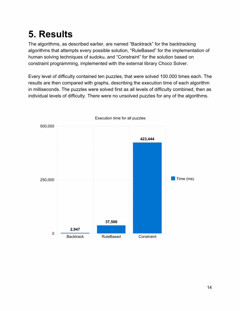
5. Results The algorithms, as described earlier, are named “Backtrack” for the backtracking algorithms that attempts every possible solution, “RuleBased” for the implementation of human solving techniques of sudoku, and “Constraint” for the solution based on constraint programming, implemented with the external library Choco Solver. Every level of difficulty contained ten puzzles, that were solved 100.000 times each. The results are then compared with graphs, describing the execution time of each algorithm in milliseconds. The puzzles were solved first as all levels of difficulty combined, then as individual levels of difficulty. There were no unsolved puzzles for any of the algorithms.

14

15

16

17

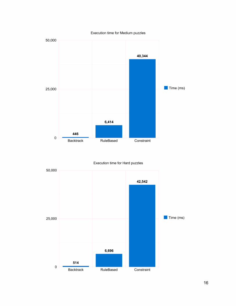
6. Discussion 6.1 Results The results show that the backtracking algorithm is by far the fastest algorithm for solving sudoku. At every level of difficulty as well as for all the levels together, it was faster than the rule based algorithm by an (approximate) factor of 10, as well as faster than the constraint based algorithm by an (approximate) factor of 100. The different levels of difficulty did not make any major difference for the solving times of the algorithms, with two exceptions. The constraint based algorithm was twice as fast for the “Medium” and “Hard” levels of difficulty. However, it was still far slower than the other two algorithms, and as such it made no major difference when compared to the other two algorithms. We found that our rule­based algorithm had no chance of beating the backtracker and thus decided to not put the time and effort into implementing more rules. We came to this conclusion since merely finding the candidates and initiating the memory for the rule­based algorithm took as long time as finding the solution using the backtracker We believe the reason constraint programming was so comparably inefficient was that we’re using a constraint based program in a non­constraint programming language. It’s likely that the transition from non­constraint to constraint language via the external library was responsible for most of the execution time. A possibility for a future report would be to implement this algorithm in a natively constraint based programming language. 6.2 Ease of implementation For inexperienced programmers, ease of implementation is worth considering. Both the constraint based algorithm and the backtracking algorithm were very easy to implement. The constraint based only proved difficult when implementing the external library itself, the code was freely available in the choco solver archives. The backtracking algorithm was clearly expressed in pseudocode in a multitude of locations, and the principle is easy enough to state that implementing it took no real effort.

18

The rule based on the other hand was more difficult to implement. With the exception of one rule, no code or pseudocode was available, and so it had to be implemented with specifications lifted from written text. The rules that we chose to implement can be considered as the most simple rules for solving sudoku. Even so it was time consuming to translate this relatively simple rules into Java code. If additional and more complex rules were to be implemented it would have required even more competence and time.

19

7. Reliability When considering the reliability of the method of comparison, there are two key aspects to consider. The first is whether the quality and quantity of test cases is sufficient to ensure that the comparison is reliable, as well as ensuring that any potential difference between the algorithms will be revealed. The second is whether the implementations of the algorithms themselves is sufficient. If the algorithms are implemented in a substandard fashion, the results may differ when compared to the correct implementation of the algorithms. 7.1 Reliability of test cases In order to ensure that there is as little possibility of bias as possible, puzzles of varying difficulty were used for the testing. In this report, the assigned level of difficulty was based on the number of different solving methods required, rather than the number of givens. This is because the number of givens are not always representative of difficulty. While this definition of difficulty is highly relevant for the rule based algorithm, for the backtrack algorithm only the number of givens is relevant, as it always tries every possible solution. Even so, the more difficult puzzles will naturally have to have less givens to avoid being too easily solved, and this method then ensures that the rule based algorithm will also experience the levels of difficulty accordingly. In order to make sure that no differences in efficiency is missed, all test cases will be ran 100.000 times each, so that any potential differences are made as obvious as possible. 7.2 Reliability of algorithm implementations The algorithm based on constraint programming is considered very reliable as it was taken directly from the creators of the constraint programming library used in this report, choco solver. In addition, the nature of constraint programming is such that very little emphasis is to be placed on the implementation of the algorithm, as it is little more than stating the nature of sudoku itself.

20

The same can be said for the backtracking algorithm. Because it is so basic and easy to express in pseudocode, the implementation is not complex enough that the reliability of the implementation is a large concern. Even if it was, it would have made no difference for the purposes of this report as backtracking was faster by a large margin, even if it was suboptimally implemented. The rule based algorithm however, is complex enough to warrant some concern. Because it is very complex there is possibility of an inefficient implementation. The rule based algorithm used for this report is based on another report that discussed the rules in detail. While the implementations of these rules is done as efficiently as we could manage, there is possibility that the final algorithm could be made even more efficient by someone with greater skill in programming. However, the current implementation is efficient enough that any difference in performance when compared to the other algorithms should be easy to observe. The memory management alone was slower than the backtracking algorithm, so it’s unlikely that the algorithm could be made faster than backtracking while programming in Java. It is important to note, however, that using a different programming language could have yielded a different result. When analyzing the huge difference in performance between the algorithms we concluded that assigning memory was a huge time sink. If a more low­level language like C was used it would allow for more liberal memory management, and possibly a different end result. 7.3 Reliability of the method The purpose of this report, as stated before, is to compare efficiency between sudoku solving algorithms. In the case of algorithm efficiency, the best way of measuring efficiency is to use the algorithm on a large number of different problems. To ensure that this is achieved, test cases were taken from a source with sufficient knowledge of sudoku. Test cases were then divided according to difficulty, to ensure no bias between the different algorithms. To ensure quantity, each puzzle was solved 100.000 times, making sure that there was no possibility of any differences being missed due to the solving times being too short to reliably compare.

21

As for the time measuring, the algorithms had to initialize their variables on every solve, which is part of why the rule based algorithm was so slow in comparison to the backtracking algorithm. It’s possible that the rule based would perform comparably better if the memory allocation only happened once per puzzle, rather than 100.000 times. However, we felt that having to initialize all variables on every solve better simulated a real world environment.

22

8. Conclusion When comparing sudoku solving algorithms written in Java, the backtracking algorithm has been proven to be superior to both the constraint algorithm as well as the rule based algorithm. The constraint solution was comparably inefficient to such a degree that it should never be considered other than for studying constraint programming in Java. The rule based algorithm was slower than backtracking even when only counting the initiation and memory allocation, and as such can never be improved to be faster than the backtracking solution by adding more rules. This of course assuming the program is written in Java. It’s possible there are ways to improve the memory management to such an extent it can outperform the backtracking algorithm, but we consider it unlikely. Since the backtracking algorithm is so efficient as well as easy to implement, we consider finding such a solution unnecessary. The conclusion we have reached is that the backtracking algorithm is the best method

for computationally solving sudoku with the Java programming language.

23

Sources:

1. Hayes, Brian (2006). "Unwed Numbers". American Scientist 94: 12–15 http://www.americanscientist.org/issues/pub/2006/1/unwed­numbers

2. Smith, David (May 15, 2005). "So you thought Sudoku came from the Land of the Rising Sun ...". The Observer. Retrieved April 2015. http://www.theguardian.com/media/2005/may/15/pressandpublishing.usnews

3. Felgenhauer, Bertram; Jarvis, Frazer (June 20, 2005), Enumerating possible Sudoku grids http://ijcsi.org/papers/IJCSI­11­2­1­247­253.pdf

4. Stanford lecture by Julie Zelensky with example of a backtracking algorithm https://www.youtube.com/watch?v=p­gpaIGRCQI

5. Moritz Lenz: Yet Another Sudoku Solver, Retrieved March 2015 http://moritz.faui2k3.org/en/yasss

6. Narendra Jussien, A to Z of SUDOKU http://www.scribd.com/doc/18469525/A­Z­Sudoku

7. Homepage for the constraint library choco­solver, Retrieved March 2015 http://choco­solver.org

8. Pseudo­code (and working example) for the backtracking algorithm, Retrieved March 2015 http://codefordummies.blogspot.se/2014/01/backtracking­solve­sudoku­in­java.html

24