Analysing the Determinants of Bank Efficiency: The Case of Italian Banks

Claudia Girardone, Philip Molyneux*, Edward P.M. GardenerSchool of Accounting, Banking and Economics, University of Wales, Bangor, Gwynedd, LL57 2DG, UK.

Abstract

This paper investigates the main determinants of Italian banks’ cost efficiency over the period 1993-96,

by employing a Fourier-flexible stochastic cost frontier in order to measure X-efficiencies and economies of

scale. Quality and riskiness of bank outputs are explicitly accounted for in the cost function and their impact on

cost efficiency levels are evaluated. The results show that mean X-inefficiencies range between 13 and 15 per

cent of total costs and they tend to decrease over time for all bank sizes. Economies of scale appear present and

significant, being especially high for popular and credit co-operative banks. Moreover, the inclusion of risk and

output quality variables in the cost function seems to reduce the significance of the scale economy estimates.

Following Spong et al. (1995) we undertake a profitability test that allows for the identification of banks that are

both cost and profit efficient. The results suggest that the most efficient and profitable institutions are more able

to control all aspects of costs, especially labour costs. Finally, we pool the data to carry out a logistic regression

model in order to examine bank- and market-specific factors that influence Italian banks’ inefficiency.

Confirming Mester (1993 and 1996), inefficiencies appear to be inversely correlated with capital strength and

positively related to the level of non-performing loans in the balance sheet. The analysis also shows that there is

no clear relationship between assets size and bank efficiency. Finally, it is possible to infer that quoted banks

seem to be on average more efficient than their non-quoted counterparts.

JEL classification: G21, D2.

Keywords: Italian banks; Cost function; Inefficiencies; Economies of scale.

* Corresponding author: School of Accounting, Banking and Economics, University of Wales Bangor, Gwynedd, Bangor

LL57 2DG (UK). E-mail: p.molyneux@bangor.ac.uk, Fax + 44 1248 364760, Tel. + 44 1248 382170.

Acknowledgements – Thanks to Professor G.B. Pittaluga from the Università degli Studi di Genova for his precious

comments and for providing the Bilbank database. We also wish to thank M. Brown, B. Casu and J. Williams from the

University of Wales, Bangor, for their valuable suggestions.

2

1. Introduction

Banking has experienced dramatic changes over the last decade or so. Deregulation,

financial innovation and automation have been major forces impacting on the

performance of the banking sector. In such a context, banks have become

increasingly concerned about controlling and analysing their costs and revenues, as

well as measuring the risks taken to produce acceptable returns.

In line with these developments, an extensive literature has evolved examining

financial firm efficiency issues (see, for a comprehensive survey, Berger and

Humphrey, 1997), and different methodological approaches have been employed to

investigate financial firm efficiency (i.e. parametric and non-parametric techniques).

However, only a handful of studies have so far investigated how risk and output

quality factors influence bank efficiency levels (for example, Mester, 1996; Berger

and Mester, 1997; Altunbas, Liu, Molyneux and Seth, 1999).

This paper has two main objectives. First it aims to extend the established

literature by examining the determinants of Italian banks’ cost efficiency over the

period 1993-96, by employing a Fourier-flexible stochastic cost frontier to evaluate

X-efficiency and scale economies. Quality and riskiness of bank output are explicitly

accounted for in the cost function and their impact on efficiency levels are evaluated

and discussed. Secondly, the paper attempts to identify the main characteristics of

efficient banks. Following the approach suggested by Spong et al. (1995) our sample

of banks is subject to a profitability test that allows us to identify institutions that are

both cost and profit efficient. Following Mester (1993 and 1996) we also use a

3

logistic regression model to examine bank- and market- specific factors which

influence banks’ inefficiency levels.

The paper is set out as follows. Section 2 provides a brief literature review on

recent developments in financial firm efficiency analysis placing particular emphasis

on various Italian studies. Section 3 outlines the methodology and section 4 reports

the results. Section 5 is the conclusion.

2. New views on bank efficiency

Over the last decade parametric studies of Italian bank cost efficiency (for example,

Baldini and Landi, 1990; Conigliani et al., 1991; Parigi et al., 1992; European

Commission, 1997; Resti, 1997; Inzerillo et al., 1999) have found evidence of

economies of scale across a wide range of bank sizes, and average X-inefficiency

levels are usually in line with those found in the international literature – typically

ranging between 15 and 20 percent. However, none of these studies have included

the level of capital and/or loan losses as arguments in the cost function to control for

risk of default and/or output quality, respectively. A relatively new approach (for

example, Hughes and Mester, 1993; McAllister and McManus, 1993; Clark, 1996;

Mester, 1996; Berger and Mester, 1997; Altunbas, Liu, Molyneux and Seth, 1999)

points to the importance of including measures of output quality and default risk on

the grounds that unless they are accounted for in the cost function, bank levels of X-

efficiencies and economies of scale may be miscalculated. In the case of Italian

banking the inclusion of these two variables could be crucial because recently credit

institutions have suffered from a dramatic increase in their level of non-performing

4

loans (NPLs). For example, Italian banks based in the south of the country recorded

NPLs (as a percentage of total loans) of 24.2 per cent in 1996 and 21.8 percent in

1997, ratios that were more than twice the national average and high by any standard

(Bank of Italy, 1998). The achievement of more competitive conditions in the Italian

banking market during the 1990s has also brought about situations of crisis for

various banking firms. During the 1993-96 period the main banks in the south of

Italy experienced substantial reductions in their net interest income and were no

longer able to cover their relatively high operating expenses and loan losses. As a

consequence, these banks either reduced their size or were acquired by larger

(healthier) banks.

Another important recent issue in bank efficiency analysis concerns the choice of

the functional form for the cost function. Studies by leading researchers in the field

(see, for example, Mitchell and Onvural, 1996; Berger and DeYoung, 1997; Berger

et al., 1997; Berger and Mester, 1997; Altunbas, Liu, Molyneux and Seth, 1999) have

abandoned the typical U-shaped translog for the sinusoidal Fourier-flexible, which

combines the stability of the translog specification near the average of the sample

data with the flexibility of the Fourier specification for observations far from the

averages. The Fourier functional form is preferred to the translog because it better

approximates the underlying cost function across a broad range of outputs.

This paper advances the literature on bank efficiency by investigating the effects

of the inclusion of risk and output quality factors in the cost function. Moreover, we

adopt a stochastic Fourier-flexible cost function to calculate X-efficiency levels and

economies of scale for a sample of Italian banks between 1993 and 1996. The paper

5

also uses a profitability test as suggested by Spong et al. (1995) to investigate the

characteristics of the most and least efficient banks in the Italian system.

3. Methodology

3.1. Input and Output Definition and Data Sample

Choosing the appropriate definition of bank output is an important issue for research

into banks’ cost efficiency. While the multiproduct nature of the banking firm is

widely recognised, there is still no agreement as to the explicit definition and

measurement of banks’ inputs and outputs. Generally, each definition of input and

output carries with it a particular set of banking concepts, which influence and limit

the analysis of the production characteristics of the industry.

The approach to output definition used in this study is a variation of the

intermediation approach, which was originally developed by Sealey and Lindley

(1977) and posits that total loans and securities are outputs, whereas deposits along

with labour and capital are inputs to the production process of banking firms. (Table

A.1 in the Appendix provides descriptive statistics on the outputs and input prices

included in our model).

The data used to construct the estimates for the cost function parameters are

derived from Bilbank, an Italian database of the Associazione Banche Private

Italiane. This database provides annual income and balance sheet data for credit

institutions belonging to different bank categories. The sample comprises an

unbalanced panel of 1,958 bank observations distributed in the following way: 545

banks in 1993, 523 in 1994, 466 in 1995 and 424 in 1996. The sample excludes: i)

6

banks that are subsidiaries of foreign banks; ii) the central institutions for each

category of banks; and iii) special credit institutions (medium- and long- term

banks).1

Our sample constitutes nearly 50 per cent of the Italian banking market in

terms of number of banks. (As displayed in Table A.2, the difference in banks’ size

across the five classes is relatively high. The groups of very big banks have

approximately 400 times the average assets of the very small banks and 40 times the

average assets of small banks).2 We also investigate efficiency of banks across

geographical regions and therefore identify those institutions located in four major

regions: north-west, north-east, centre, south and islands.3

3.2. Stochastic Cost Frontier Model, X-Efficiencies and Economies of Scale

Researchers investigating bank cost efficiency postulate a relationship between costs,

input prices and output quantity. This relationship is based on the duality concept

between production and cost functions. The production function ( )XQQ =

summarises the technology of a firm, that is the existing relationship between inputs,

1 It should also be noted that in the empirical analysis most of the estimation is carried out using the FRONTIER

4.1 and TSP 4.0 packages. Since FRONTIER 4.1 does not tolerate missing values, banks with incomplete

accounting data could not be included in the data sample (Coelli, 1996 and Coelli et al., 1998).

2 The Bank of Italy categorises banks according to five size groups: very big; big; medium; small and very small.

3 These different regions are defined as follows: 1) North-West: Liguria, Lombardia, Piemonte, Valle d’Aosta; 2)

North-East: Emilia-Romagna, Friuli-Venezia Giulia, Trentino Alto Adige, Veneto; 3) Centre: Lazio, Marche,

Toscana, Umbria; 4) South and Islands: Abruzzo, Basilicata, Calabria, Campania, Molise, Puglia, Sardegna,

Sicilia. It should be noted that a bank was assigned to a given region if, over the period, it had its head office in

that area.

7

X, and outputs, Q. The cost function ( )PQTCTC ,= shows the relationship between

total production costs, TC, and the prices of variable inputs. The duality condition

between the production and the cost function ensures that they contain the same

information about production possibilities and that there is a unique correspondence

between both functions. Moreover, observable production plans and cost levels

usually do not follow from perfectly rational and efficient decisions. On the contrary,

such factors as errors, lags between the choice of the plan and its implementation,

inertia in human behaviour and distorted communications and uncertainty are

amongst the factors that might cause X-inefficiencies to drive real data away from

the optimum (Resti, 1997).

This study employs the stochastic cost frontier approach to generate estimates of

X-efficiencies for each bank over the years 1993-96 along the lines first suggested by

Aigner et al. (1977) and Meeusen and van den Broeck (1977). For the i-th firm, the

single equation cost function model is represented by ( ) ijii TCTC ε+= BPQ ;,lnln ,

where TCi is the observed total cost of production for bank i, Qi is the vector of

banking output for bank i, Pj is the vector of input prices for bank j and B is a vector

of parameters. ( )BPQ ;,ln jiTC is the predicted log cost function of a cost minimising

bank operating at ( )BPQ ,, ji . Finally εi is a two-components error term that for the i-

th firm can be written as follows:

iii uv +=ε (1)

where vi is a two-sided error term representing statistical noise which is assumed to

be independently and identically distributed; and ui is a non-negative (or one-sided)

random variable representing inefficiency and assumed to be distributed

8

independently of the vi. It is also assumed that the vi are normally distributed with

mean zero and variance σ v2 , and the ui are the absolute values of a variable that is

normally distributed with mean µ and variance 2uσ .

In the present study banks’ data over the period 1993-96 are organised in a panel.

Specifically, we employ the Battese and Coelli (1992) model of a stochastic frontier

function for panel data with firm effects which are assumed to be distributed as half-

normal random variables (that is, with µ=0)4 and are also permitted to vary

systematically with time. Therefore, it is possible to express this model as

itititit uvxTC ++= β , [with i = (1,2, ..., N) and t = (1,2, ..., T)], where TCit is (the

logarithm) of the total costs for the i-th firm in the t-th time period; xit is a k×1 vector

of (transformations of the) input and output quantities of the i-th firm in the t-th time

period; β is the vector of unknown parameters; and the vit and uit are defined as

above, with uit = {exp[η(t-T)]}, where η is an unknown scalar parameter to be

estimated that represents the hypothesis about the evolution or steadiness of

individual inefficiencies over the period under study.

Moreover, the parameterisation of Battese and Corra (1977) is employed, who

replaced σ v2 and σ u

2 with σ σ σ2 2 2= +v u and ( )γ σ σ σ= +u v u2 2 2 .5 As recently

emphasised by Coelli et al. (1998) the γ-parameterisation has an advantage in

4 There are many variations on this assumption in the literature (for details, see Greene, 1993 and Coelli et al.,

1998).

5 In the literature, the likelihood function has often been expressed in terms of the two variance parameters

222uv σσσ += and 22

vu σσλ ≡ (Aigner et al., 1977; Jondrow et al., 1982; Coelli, 1996). See also Battese and

Coelli (1993) and Coelli et al. (1998) for the log-likelihood function of the model used here given these

distributional assumptions.

9

seeking to obtain the maximum likelihood estimates because the parameter space for

γ can be searched for a suitable starting value for the iterative maximisation

algorithm involved. In particular, a value of γ of zero indicates that the deviations

from the frontier are due entirely to noise, while a value of one would indicate that

all deviations are due to inefficiency.

As concerns the choice of the functional form for the cost function, this study

employs a Fourier-flexible form because it is a global approximation that has proved

to dominate the commonly specified translog form (see, for example, McAllister and

McManus, 1993; Mitchell and Onvural, 1996; Berger et al., 1997; Altunbas, Liu,

Molyneux and Seth, 1999). The resulting mixed cost function can be written as:

[ ] ( ) ( )[ ]

( ) ( )[ ] ii ij

ikjk

kjiijkjiij

i jjiijjiij

iiiii

ksjj

jsii

is

jj

jkii

iki j

jiij

sskki i j

jiijj

jiij

skj

jjii

i

zzzzzz

zzzzzz

SKSPSQ

KPKQPQ

SSKKPPQQ

skPQTC

εθλ

θλθλ

τβα

βαρ

ττγδ

ττβαα

+++++++

+++++++

++++

++++

+

+++

+++++=

∑∑∑

∑∑∑

∑∑

∑∑∑∑

∑ ∑∑∑

∑∑

= ≥≠≥

= ==

==

=== =

= = ==

==

2

1

2 2

2

1

2

1

4

1

3

1

2

1

3

1

2

1

2

1

3

1

2

1

3

1

3

1

2

1

3

1

2

10

sincos

sincossincos

lnlnlnlnlnln

lnlnlnlnlnln

lnlnlnlnlnlnlnln

21lnlnlnlnln

(2)

where TC is a measure of the normalised costs of production, comprising operating

costs and financial costs (interest paid on deposits); 1Q and 2Q are output quantities,

that is total loans and total securities, respectively; 1P is the normalised price of

labour; 2P is the normalised price of deposits; K is the level of financial capital; S is

10

the ratio of NPLs to total loans; α β δ γ, , , ,ρ , λ, θ ,τ are parameters to be estimated;

and εi is the two-component error term as defined in (1). Moreover, the iz are

adjusted values of the natural log of output iQln so that they span the interval

[ ]ππ 29,.21. ∗∗ . In particular, the formula for iz used here is ( iQa ln2. ∗+∗− µµπ ),

where [ ]ba, is the range of iQln and ( ) ( )ab−∗−∗≡ ππµ 21.29. .

The Fourier-flexible form is a global approximation because the terms such as

izcos , izsin , iz2cos , iz2sin are mutually orthogonal over the [ ]π2,0 interval, so

that each additional term can make the approximating function closer to the true path

wherever it is most needed. As observed by Gallant (1981), by restricting the iz to

span the interval [ ]ππ 29,.21. ∗∗ , the approximation problems arising near the

endpoints are reduced.

In addition, standard symmetry has to be imposed on the translog portion of the

function: jiij δδ = and jiij γγ = , where )2,1( =i and )3,2,1( =j , and the following

linear restrictions on (2) are necessary and sufficient for linear homogeneity in factor

prices: ∑=

=3

1

1j

jβ ; ∑=

=3

1

0i

ijγ ; ∑=

=3

1

0j

ijρ ; ∑=

=3

1

0i

jkβ ; ∑=

=3

1

0i

jsβ . In accordance with

the assumed constraint of linear homogeneity in prices, TC, P1 and P2 are normalised

by the price of capital, 3P . It is also important to mention that consideration of input

share equations embodying Shephard’s Lemma restrictions is excluded in order to

allow for the possibility of allocative inefficiency (see, for example, Berger and

Mester, 1997). The Fourier terms are included only for the outputs, leaving the input

price effects to be described solely by the translog term (see, for example, Berger et

al., 1997 and Altunbas, Liu, Molyneux and Seth, 1999). The Fourier terms for the

11

input prices are also excluded in order to conserve the limited number of Fourier

terms for the output quantities used to measure economies of scale. The input prices

also show very little variation, thereby providing greater justification for our

methodological approach.

In this research the parameters of the stochastic frontier cost function, defined by

eq. (2), are estimated using the Maximum-Likelihood (ML) approach. For instance,

the ML estimates of β and γ are obtained by finding the minimum of the log-

likelihood function as specified in Coelli et. al (1998). The nature of this log-

likelihood function given the distributional assumptions on v and u can also be found

in Battese and Coelli (1992).

Once the model is estimated, bank level measures of X-efficiencies are calculated

using the residuals and are usually given by the mean of the conditional distribution

of ui given iε . For the half-normal stochastic model the E(ui|εi) is considered as a

consistent estimator for individual X-efficiencies (Coelli et al., 1998). The resulting

cost efficiency ratio may be thought of as the proportion of costs or resource that are

used efficiently. For example, a bank with a cost efficiency of 0.80 is 80 per cent

efficient or equivalently wastes 20 per cent of its costs relative to a best practice firm

facing the same conditions.

A natural way to express the extent of scale economies is the proportional

increase in cost resulting from a small proportional increase in the level of output,

that is the elasticity of total cost with respect to output. The degree of economies of

12

scale (SCALE) used here is given by ∑=

=m

i iQ

TCSCALE

1 ln

ln

∂∂

which represents the sum

of individual cost elasticities.6 This can be rewritten as:

( ) ( )

( ) ( )

( ) ( )∑∑∑

∑∑

∑∑∑

∑ ∑∑ ∑∑

= ≥≠≥

= =

===

= = = = =

++−+++

++−++

+−+++

+++=

2

1

2 2

2

1

2

1

2

1

2

1

2

1

2

1

2

1

2

1

2

1

3

1

cossin

cossin

cossinlnln

lnln

i ijikjk

kjiijkkjiijk

i jjiijjiij

iiiii

iis

iik

i i j i jjijjiji

zzzzzz

zzzz

zzSK

PQSCALE

θλ

θλ

θλαα

ρδα

(3)

where there are economies of scale if SCALE<1, constant returns to scale if

SCALE=1, and diseconomies of scale if SCALE>1. The degree of scale economies is

computed by using the mean values of output, input prices and risk and output

quality variables.

3.3. Profitability Test and Correlates with Inefficiency

Following Spong et al. (1995), we subject our cost efficiency measures derived from

the Fourier model to a profitability test. This is undertaken in order to identify banks

that are both cost – and profit – efficient. This approach is taken because the cost side

may provide inaccurate rankings of efficiency because a seemingly cost inefficient

bank might be offsetting higher expenses with higher revenues. Moreover, this test

6 Evanoff and Israilevich (1985) distinguish between scale elasticity and scale efficiency where the former is

measured as in equation (3) and the latter is measured as the change in output required to produce at minimum

efficient scale. Throughout this paper reference to economies and diseconomies of scale relates to scale

elasticities.

13

provides an alternative to some of the consistency conditions recently suggested by

Bauer et al. (1997).

It follows that banks which do well on both cost efficiency and profitability tests

will comprise the “most efficient” bank category; banks that fare poorly on the two

tests are in the “least efficient” category. The two groups, comprising the most

efficient and least efficient banks were partitioned in the following way: 1) most

efficient group: banks that rank in the upper quartile of Italian banks on the cost

efficiency estimates and rank in the upper half in terms of ROA (return on assets),

and 2) least efficient group: banks that rank in the bottom quartile on the cost

efficiency estimates and rank in the bottom half in term of ROA. Subsequently, we

analyse the financial characteristics of efficient and inefficient banks by carrying out

a comparison between the major sources of income and expenses as well as several

other financial ratios for the year 1996.

Lastly, in order to investigate possible determinants of bank efficiency, firm-

specific measures of inefficiency derived exclusively from the model excluding risk

and output quality variables – that is, equation (2) without the variables K and S –,

are regressed on a set of independent variables relevant to the banking business. This

set of potential correlates with bank inefficiency is chosen in such a way that many

aspects of banking activities are considered: for instance, bank size, market

characteristics, geographic position, capital, performance and retail activities (see

also Mester, 1996; Berger and Mester, 1997; and Altunbas, Liu, Molyneux and Seth,

1999). A logistic functional form rather than a linear regression model is used

because the values of the inefficiency estimates, ( )iiuE εˆ , range between 0 and 1 (for

applications of this technique to the banking system, see Mester, 1993 and 1996).

14

4. Results

4.1. Structural Tests

Structural tests are undertaken to see if the cost function that included the risk and

output quality variables differs significantly from the standard cost frontier

specification, the translog form, and the models including individual risk and quality

variables.

Table A.3 in the Appendix reports the likelihood ratio test statistics and shows

that the cost frontier including risk and quality variables provides the best fit to the

data. More specifically the cost function that includes the risk and quality variables

(RQCF) differs significantly from the standard model (CF) since the likelihood ratio

test rejects the hypothesis that the two models are not significantly different.

With particular regard to the choice of the functional form for the cost function,

the translog model is rejected at the 0.01 per cent level, thus supporting the choice of

the Fourier-flexible function. Similarly, the models excluding individual risk and

quality variables are all rejected against our model defined in (2) at the 0.01 per cent

level.

4.2. X-Efficiencies and Economies of Scale

Tables 1 and 2 report the average X-efficiency levels for banks grouped by size

classes, geographical areas (a bank is assigned to a given region if it has its head

office in that area) and bank types (the category “commercial banks” includes those

banks that are not savings, popular or credit co-operative banks). We distinguish

between different types of banks because mutual banks (savings and co-op banks)

15

may have different managerial objectives compared with commercial banks and this

could be reflected in their cost efficiency. For instance, it could be the case that

mutual banks have objectives other than cost minimisation – such as serving the local

community and maximising returns to members.

Tables 1 & 2 here

Average inefficiency levels range between approximately 13 and 15 per cent.

Similar figures can be found in various recent studies of Italian banks (see, for

example, Allen and Rai, 1996; European Commission, 1997) and, although

differences are not large, the most efficient banks seem to be the big, medium and

very small banks. Moreover, X-inefficiency levels seem to decrease over time and

for all sizes of banks.

When the X-efficiency results are grouped according to banks operating in

different geographical areas, it appears that the lowest efficiency levels are generally

found for banks having their head office in the centre and south of the country, thus

confirming the apparent existence of significant disparities among geographical

regions. Finally, according to the different bank types, it is possible to observe that

on average the better performing banks seem to be the credit co-operatives together

with popular banks, possibly reflecting a greater homogeneity of the co-operative

banking sector. Altunbas, Evans and Molyneux (1999) found similar results for

German banks and they argue that mutual banks tend to have a lower cost of funds

than other bank types due, for example, to their (possible) local monopolies.

16

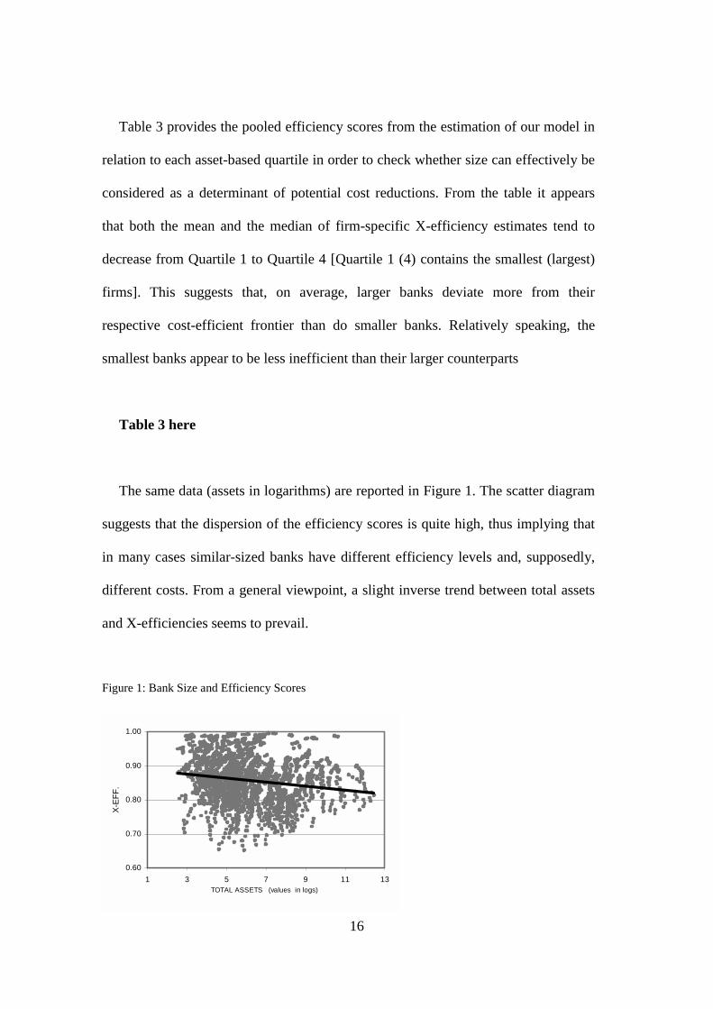
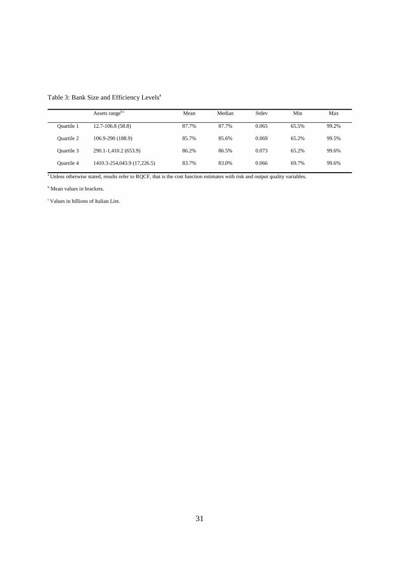
Table 3 provides the pooled efficiency scores from the estimation of our model in

relation to each asset-based quartile in order to check whether size can effectively be

considered as a determinant of potential cost reductions. From the table it appears

that both the mean and the median of firm-specific X-efficiency estimates tend to

decrease from Quartile 1 to Quartile 4 [Quartile 1 (4) contains the smallest (largest)

firms]. This suggests that, on average, larger banks deviate more from their

respective cost-efficient frontier than do smaller banks. Relatively speaking, the

smallest banks appear to be less inefficient than their larger counterparts

Table 3 here

The same data (assets in logarithms) are reported in Figure 1. The scatter diagram

suggests that the dispersion of the efficiency scores is quite high, thus implying that

in many cases similar-sized banks have different efficiency levels and, supposedly,

different costs. From a general viewpoint, a slight inverse trend between total assets

and X-efficiencies seems to prevail.

Figure 1: Bank Size and Efficiency Scores

0.60

0.70

0.80

0.90

1.00

1 3 5 7 9 11 13TOTAL ASSETS (values in logs)

X-E

FF

.

17

Table 4 reports economies of scale estimates for each year together with their

significance levels. The results seem to confirm that big and medium banks show

high and significant scale economies in the majority of cases, and very small banks

also appear to enjoy substantial economies. Very big banks do not appear to

experience potentially realisable scale economies in the years under study and mainly

exhibit constant returns to scale.

Table 4 here

Table 5 shows scale economy estimates according to different bank types and

geographic areas. The table reveals several interesting patterns: i) commercial banks

show high and significant economies of scale especially in the northern part of the

country; ii) savings banks appear on average the less likely to gain from potential

scale economies; and iii) popular and credit co-operative banks appear best able to

exploit cost reductions in terms of economies of scale.

Table 5 here

Finally, if we compare the results on the X-efficiencies (Table 1) and economies

of scale (Table 4) derived from the cost function including risk and output quality

factors (RQCF) with those obtained from the standard cost function (CF) we find that

X-efficiency results are similar. However, it does appear to be the case that the extent

of scale economies seems to be overstated if risk and quality factors are not included

18

in the cost function specification. This result is broadly in accordance with the recent

findings of Berger and Mester (1997) and Altunbas, Liu, Molyneux and Seth (1999).

4.3. Profitability Test and Correlates with Inefficiency

So far our analysis has only focused on cost efficiency. Spong et al. (1995),

however, note that it is important to combine both cost efficiency estimates with a

profitability test so as to evaluate financial firm efficiency. This is because one needs

to evaluate banks’ ability to use resources effectively in producing products and

services (cost efficiency), and their skill at generating income from these services

(profitability). Following Spong et al. (1995) we partition our sample of banks into

two categories – the most and least efficient – in terms of their cost efficiency and

profits performance. The most (least) efficient banks are those that rank in the upper

(lower) quartile according to the cost efficiency estimates and in the upper (lower)

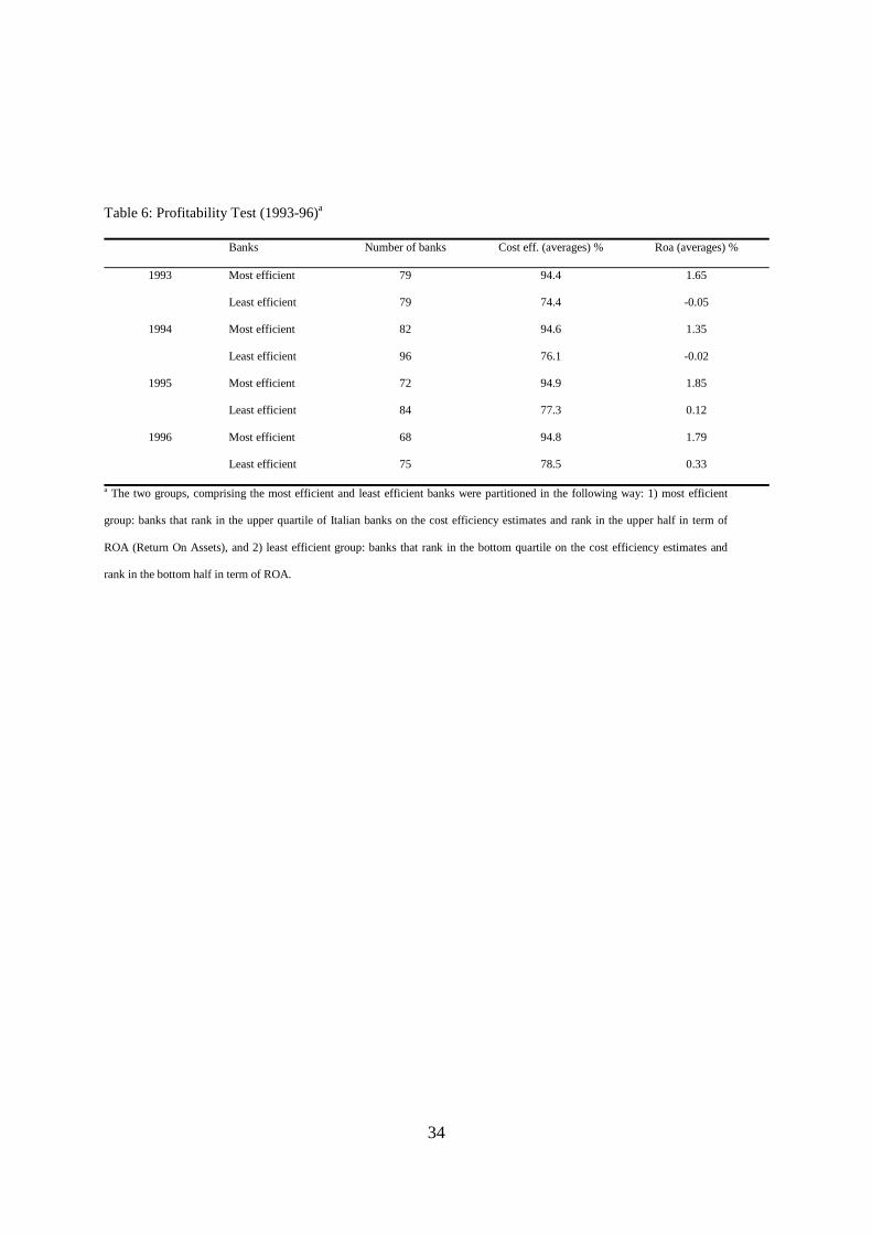
half in terms of return on assets. Table 6 shows the number of banks and their

efficiency and profitability characteristics according to the aforementioned

partitioning.

Table 6 here

For the four years under study, an average of 75 banks satisfy the selection criteria

for the most efficient group and 84 banks are classified in the least efficient group.

The mean bank in the least efficient group has a cost efficiency of only 0.77, which

indicates that the bank with the highest efficiency in the sample could have produced

the same amount of output as the least efficient bank at only 77 per cent of their cost.

19

In contrast, the average cost efficiency level for the most efficient banks is

approximately 0.95, thus indicating less disparity with the “best” bank in the sample.

Moreover, as an average for the four years, the ROA for the most efficient banks is

equal to 1.66% compared with 0.09% for the poorest performers.

In order to analyse the financial characteristics of efficient and inefficient banks

Table 7 shows a comparison between the major sources of income and expenses as

well as several other financial ratios for these banks. The table reveals how efficient

and inefficient banks differ. The table also shows financial characteristics for the

sample “all banks” and also for a sub-sample of “large banks only”. This latter group

includes the following bank sizes: very big, big, medium and small (see Table A.2

for their assets size range). The choice of creating such a sub-sample is motivated by

the fact that the relatively large number of very small banks found in the least and

most efficient bank categories could bias our interpretation of the results.

Table 7 here

On the earnings side, the advantages held by the most efficient banks seems to

relate to their income generating capacity and, as expected, expenses control.

Focusing on the sample “all banks” the most efficient group has, for instance, an

advantage over inefficient banks in terms of higher interest received on assets. On

the other hand, the most inefficient banks have relatively high non-interest revenues

compared with the most efficient banks, thus suggesting that there might be some

differences in the way the two groups generate income. However, these results

20

change if the very small banks are excluded from the sample, which shows a greater

importance of non-interest income for the most efficient group.

As concerns the expense side, the most efficient and least efficient banks show

similar interest expenses. This means that the most efficient banks do not have

important advantages in funding costs, and therefore they are achieving their

performance by other means, other factors being equal. Furthermore, it seems

apparent that efficient banks are more effective in controlling operating costs, and

particularly staff expenses.

With regard to their balance sheet structures, in 1996 the most efficient banks hold

more securities and have higher levels of equity than their inefficient counterparts,

thus providing a high level of protection to their customers. Moreover, the most

efficient banks appear to have better asset quality, thereby implying that they are

assigning more attention and resources to loan origination, monitoring and other

credit judgement activities.

Finally, in order to investigate the possible determinants of bank efficiency, firm-

specific X-inefficiencies are regressed on a set of independent variables relevant to

the banking business. As stressed by Mester (1996), the findings are intended mainly

to indicate where banks might look for clues toward increasing their efficiency. As

shown in Table 8 the estimates indicate that different variables significantly correlate

with inefficiencies in the Italian banking sector. Again our sample banks are divided

into large banks (very big, big, medium and small banks), and very small banks.

Table 8 here

21

In accordance with Mester’s findings (1993 and 1996), inefficiencies are always

inversely correlated with financial capital. On the one hand, this is quite predictable

since banks with low inefficiency will tend to have more profits as they will be able

(holding dividends constant) to retain more earnings as capital. However, this result

should not be interpreted as saying that if a bank increases its capital/assets ratio then

its inefficiency will decrease. As Mester (1996) points out, this could also be

explained as an indication that higher capital ratios may prevent moral hazard both

for the bank and its managers. Moreover, inefficiencies are usually inversely

correlated with bank performance variables, although this relationship is

insignificantly different from zero.

With regard to the coefficient for the level of NPLs, it is always positively related

to bank inefficiency. In fact, higher efficiency is expected to be correlated with better

credit risk evaluation (see also Mester, 1993; Berger and DeYoung, 1997; Altunbas,

Liu, Molyneux and Seth, 1999). Over the period 1993-96, inefficient banks also

tended to have a higher intensity of retail banking business, a higher number of

branches than efficient banks, and a higher interest margin to assets ratio. These

factors appear to be important in determining variations in efficiency among size

classes.

The results concerning the relationship between total assets size and bank

efficiency are mixed. The coefficient is not significantly different from zero for both

the ‘all’ and ‘large bank’ categories. These findings show that there is no statistical

evidence that larger banks are more or less X-efficient than their smaller

counterparts. In fact, from the results it is possible to see that an inverse relationship

between assets size and inefficiency appears only to hold within a specific bank size

22

group (i.e. very small banks). The results also indicate that quoted banks are, on

average, more efficient than their non-quoted counterparts. Finally, the significance

and negative sign of the dummy variable for private banks suggests that, at least

large private banks tend to have lower levels of inefficiency.

5. Conclusions

During the 1990s the Italian banking system has experienced a decline in

profitability brought about by the fall in interest margins and persistently high levels

of staffing costs. In addition, adverse macroeconomic conditions have lead to a

substantial increase in non-performing loans especially for banks located in specific

geographical areas of the country.

The response of the banking system to these pressures has been to undertake a

substantial consolidation movement resulting in an increase in the number of banking

groups and promoting the privatisation process. Evidence on efficiency and

profitability gains following M&A activities in Italy are mixed (see for example

Resti, 1998; Focarelli et al., 1999). As to the privatisation process, by the end of

1993 over 90 per cent of those banks previously acting as public foundations had

become joint-stock companies. Despite this only some 30 banks are publicly listed

and more than 50 per cent of the banking system is still in public hands (Resti, 1998).

The aim of this paper was to provide an empirical analysis of the cost efficiency

of the Italian banking sector over the period 1993-96 taking into account the risks

associated with banks’ operations. We found that mean X-inefficiency levels range

between 13 and 15 per cent of their total costs and they tend to decrease over time

23

and for all sizes of banks. Similarly, economies of scale appear present and

significant in the Italian banking system when considered as a whole. These are quite

important results if we consider that during 1993-96 the process of consolidation and

restructuring of the system has aimed at gradually increasing banks’ size.

The most cost efficient banks, both in terms of X-efficiency and economies of

scale, are big and medium sized banks generally located in the northern part of the

country. Furthermore, the results for credit co-operative banks confirm other studies

that economies of scale can be particularly high at a local level and for very small

banks because of possible local monopolies.

We also compare the results on X-efficiencies and economies of scale derived

from the cost function including risk and output quality factor and the standard cost

function. In line with recent findings by Berger and Mester (1997) and Altunbas, Liu,

Molyneux and Seth (1999), the X-efficiency estimates are similar across the two

different cost function specifications. In contrast, the level and significance of scale

economy estimates appears lower as a result of the inclusion of risk and output

quality factors in the cost function.

Following the profitability test as suggested by Spong et al. (1995), the main

differences between the “most efficient” and “least efficient” bank seem to be mainly

related to staff expenses. In the context of important technological improvements in

banks’ productive processes, this suggests an urgent need for greater labour market

flexibility and the consequent substitution of labour for capital. Moreover, inefficient

banks always appear to have lower levels of equity/assets and higher levels of non-

performing loans.

24

Finally, we pooled the data to carry out a logistic regression model in order to

examine bank- and market-specific factors that influence banks’ efficiency.

Confirming Mester (1993 and 1996), inefficiencies appear to be inversely correlated

with capital and positively related to the level of non-performing loans. This latter

finding suggests that efficient banks are assigning more attention and resources to

loan origination, monitoring and other credit judgement activities. Interestingly, over

the period 1993-96 inefficient banks also tended to have (on average) a greater retail

banking orientation, higher interest margins and more branches compared with their

efficient counterparts.

Finally, the analysis also shows that there is no clear relationship between assets

size and bank efficiency. However, from the results it is possible to infer that quoted

banks, on average, appear to be more efficient than their non-quoted counterparts.

25

Appendix

Table A.1: Variable DescriptionVariables Symbol Description

Total Costs TC Staff expenses + other non-interest expenses + interest paid

Output 1 Q1 Total customer loans

Output 2 Q2 Other earning assets

Input Price 1 P1 Staff expenses / average number of personnel

Input Price 2 P2 Interest expenses / total customer deposits

Input Price 3 P3 Other non-interest expenses / total fixed assets

Financial Capital K Total equity

Asset Quality S Non-performing loans / total loans

Table A.2: Distribution of Sample Banks by Average Assetsa,b,c

Bank size 1993 1994 1995 1996 Mean

Very Big 141,816.2 (8) 140,645.1 (8) 142,232.2 (8) 136,131.1 (8) 140,206.2 (8)

Big 35,360.8 (12) 34,875.7 (12) 37,597.1 (12) 37,755.9 (12) 36,397.4 (12)

Medium 11,717.8 (25) 12,000.9 (25) 12,770.4 (22) 13,844.6 (21) 12,583.4 (23)

Small 3,849.2 (67) 3,528.9 (62) 3,708.9 (60) 3,853.0 (58) 3,735.0 (62)

Very Small 364.1 (433) 342.4 (416) 365.0 (364) 392.2 (325) 365.9 (385)

a Billions of Italian Lire.

b In brackets the number of banks.

c All monetary aggregates are expressed at 1996 prices.

Table A.3: Structural Testsa,b

Test Performed

[versus RQCF] Test Statistics

Degrees

of Freedom

Critical

Value 201.χ

Outcome

CF = Standard cost frontier 98.4 k = 13 27.69 Rejected

Translog formc 120 k = 14 29.14 Rejected

Npls/Total loans only (S only) 23 k = 7 18.48 Rejected

Equity only (K only) 83.4 k = 7 18.48 Rejected

a The likelihood ratio statistics is calculated as ( )[ ] ( )[ ]{ }10 lnln2 HLHL −− were ( )0HL and ( )1HL are the values of the

likelihood function under the null and the alternative hypotheses, 0H and

1H , respectively.

b RQCF = cost function estimates with risk and output quality variables. The CF (standard cost frontier) is like the model specified

in eq. (2) excluding K and S (risk and output quality variables, respectively).

c The translog form tested here includes K and S.

26

References

Aigner, D.J., Lovell C.A.K. and P. Schmidt, 1977, Formulation and Estimation of Stochastic Frontier

Production Function Models, Journal of Econometrics 6, 21-37.

Allen, L. and A. Rai, 1996, Operational Efficiency in Banking: An International Comparison, Journal of

Banking and Finance 20, 655-672.

Altunbas, Y., Evans L. and P. Molyneux, 1999, Bank Ownership and Efficiency, Journal of Money,

Credit and Banking, forthcoming.

Altunbas, Y., Liu M.H., Molyneux P. and R. Seth, 1999, Efficiency and Risk in Japanese Banking,

Journal of Banking and Finance, forthcoming.

Baldini, D. and A. Landi, 1990, Economie di scala e complementarietà di costo nell’industria bancaria

italiana, L’industria 1, 25-45.

Bank of Italy, 1998, Summary Reports on Economic Developments in the Italian Regions in 1997, Rome.

Battese, G.E. and T.J. Coelli, 1992, Frontier Production Functions, Technical Efficiency and Panel Data:

With Application to Paddy Farmers in India, Journal of Productivity Analysis 3, 153-169.

Battese, G.E. and T.J. Coelli, 1993, A Stochastic Frontier Production Function Incorporating a Model for

Technical Inefficiency Effects, Working Paper in Econometrics and Applied Statistics, Department of

Econometrics, University of New England, Armidale 93-69.

Battese, G.E. and G.S. Corra, 1977, Estimation of a Production Frontier Model: With Application to the

Pastoral Zone of Eastern Australia, Australian Journal of Agricultural Economics 21, 169-179.

Bauer, P.W., Berger A.N., Ferrier G.D. and D.B. Humphrey, 1997, Consistency Conditions for

Regulatory Analysis of Financial Institutions: A Comparison of Frontier Efficiency Methods,

Finance and Economics Discussion Series, Federal Reserve Board 97-50.

Berger, A.N. and R. DeYoung, 1997, Problem Loans and Cost Efficiency in Commercial Banks, Journal

of Banking and Finance 21, 849-870.

Berger, A.N. and D.B. Humphrey, 1997, Efficiency of Financial Institutions: International Survey and

Directions for Future Research, Finance and Economics Discussion Series, Federal Reserve Board 97-

11.

Berger, A.N., Leusner J.H. and J. Mingo, 1997, The Efficiency of Bank Branches, Journal of Monetary

Economics 40, 141-162.

27

Berger, A.N. and L.J. Mester, 1997, Inside the Black Box: What Explains Differences in the Efficiencies

of Financial Institutions?, Journal of Banking and Finance 21, 895-947.

Clark, J.A., 1996, Economic Cost, Scale Efficiency and Competitive Viability in Banking, Journal of

Money, Credit and Banking 28, 342-364.

Coelli, T.J., 1996, A Guide to FRONTIER Version 4.1: A Computer Program for Stochastic Frontier

Production and Cost Function Estimation, Working Paper, Centre for Efficiency and Productivity

Analysis 96-7.

Coelli, T.J., Prasada Rao D.S. and G. Battese, 1998, An Introduction to Efficiency and Productivity

Analysis, Norwell, Kluwer.

Conigliani, C., De Bonis R., Motta G. and G. Parigi, 1991, Economie di scala e di diversificazione nel

sistema bancario italiano, Temi di Discussione, Banca d’Italia 150.

European Commission, 1997, Credit Institutions and Banking, The Single Market Review, Subseries II:

Impact on Services, Vol. 3, Kogan Page-Earthscan, London.

Evanoff, D.D. and P.R. Israilevich, 1995, Scale Elasticity versus Scale Efficiency Southern Economic

Journal 61, 1036-1046.

Focarelli, D., Panetta F. and C. Saleo, 1999, Why Do Banks Merge: Some Empirical Evidence from Italy,

Banca d’Italia, forthcoming.

Gallant, A. R., 1981, On the Bias in Flexible Functional Forms and an Essentially Unbiased Form: The

Fourier Flexible Form, Journal of Econometrics 15, 211-245.

Greene, W.H., 1993, The Econometric Approach to Efficiency Analysis, in: H.O. Fried, Lovell C.A.K.

and S.S. Schmidt, eds., The Measurement of Productive Efficiency: Techniques and Applications

(Oxford, Oxford University Press) 68-119.

Hughes, J.P. and L.J. Mester, 1993, A Quality and Risk-Adjusted Cost Function for Banks: Evidence on

the ‘Too-Big-To-Fail’ Doctrine, Journal of Productivity Analysis 4, 293-315.

Inzerillo, U., Morelli P. and G.B. Pittaluga, 1999, Deregulation and Changes in European Banking

Industry, in: CEPS-CSC, Regulatory Reform for the Better Functioning of Markets, forthcoming.

Jondrow, J., Lovell C.A.K., Materov I.S. and P. Schmidt, 1982, On the Estimation of Technical

Inefficiency in the Stochastic Frontier Production Function Model, Journal of Econometrics 19, 233-

238.

28

McAllister, P.H. and D. McManus, 1993, Resolving the Scale Efficiency Puzzle in Banking, Journal of

Banking and Finance 17, 389-405.

Meeusen, W. and J. van den Broeck, 1977, Efficiency Estimation from Cobb-Douglas Production

Functions with Composed Error Term, International Economic Review 18, 435-444.

Mester, L.J., 1993, Efficiency in the Savings and Loan Industry, Journal of Banking and Finance 17, 267-

286.

Mester, L.J., 1996, A Study of Bank Efficiency Taking into Account Risk Preferences, Journal of

Banking and Finance 20, 1025-1045.

Mitchell, K. and N.M. Onvural, 1996, Economies of Scale and Scope at Large Commercial Banks:

Evidence from the Fourier Flexible Functional Form, Journal of Money, Credit, and Banking 28, 178-

199.

Parigi, G., Sestito P. and U. Viviani, 1992, Economie di scala e diversificazione nell’industria bancaria:

ruolo dell’eterogeneità tra imprese, Temi di Discussione, Banca d’Italia 174.

Resti, A., 1997, Evaluating the Cost Efficiency of the Italian Banking Market: What Can Be Learned

from the Joint Application of Parametric and Non-parametric Techniques, Journal of Banking and

Finance 21, 221-250.

Resti, A., 1998, Can Mergers Foster Efficiency? The Italian Case, Journal of Economics and Business 50,

157-169, March/April.

Sealey, C.W. and J.T. Lindley, 1977, Inputs, Outputs and a Theory of Production and Cost at Depository

Financial Institutions, Journal of Finance 32, 1251-1266.

Spong, K., Sullivan R. and R. DeYoung, 1995, What Makes a Bank Efficient? A Look at Financial

Characteristics and Bank Management and Ownership Structure, Financial and Industry

Perspectives, Federal Reserve Bank of Kansas City, 1-19, December.

29

Table 1: Average Values of X-Efficiency Grouped by Size Classesa

1993 1994 1995 1996 1993 1994 1995 1996

RQCF RQCF RQCF RQCF CF CF CF CF

Very big 83.2% 84.0% 84.7% 85.4% 81.2% 81.8% 82.3% 82.8%

Big 85.1% 85.8% 86.4% 87.1% 85.2% 85.6% 86.1% 86.5%

Medium 85.6% 86.2% 87.2% 87.5% 85.9% 86.3% 87.0% 87.0%

Small 81.1% 82.0% 82.8% 83.5% 81.6% 82.3% 82.8% 83.3%

Very small 85.2% 86.2% 87.0% 87.6% 85.4% 86.1% 86.7% 87.1%

a RQCF= cost function estimates with risk and output quality variables; CF = standard cost function estimates.

30

Table 2: Average Values of X-efficiency Grouped by Bank Types and Geographical Areasa

1993 1994 1995 1996

By region North-west 86.4% 87.6% 88.0% 88.4%

North-east 84.9% 85.8% 87.0% 87.4%

Centre 83.6% 84.5% 85.0% 85.3%

South and islands 83.5% 84.4% 85.2% 86.1%

By bank type Commercial 80.5% 81.8% 82.6% 83.2%

Savings 82.3% 83.2% 84.1% 85.0%

Popular 84.1% 85.6% 86.6% 87.1%

Credit co-op. 86.4% 87.1% 87.7% 88.2%

a Unless otherwise stated, results refer to RQCF, that is the cost function estimates with risk and output quality variables.

31

Table 3: Bank Size and Efficiency Levelsa

Assets rangeb,c Mean Median Stdev Min Max

Quartile 1 12.7-106.8 (58.8) 87.7% 87.7% 0.065 65.5% 99.2%

Quartile 2 106.9-290 (188.9) 85.7% 85.6% 0.069 65.2% 99.5%

Quartile 3 290.1-1,410.2 (653.9) 86.2% 86.5% 0.073 65.2% 99.6%

Quartile 4 1410.3-254,043.9 (17,226.5) 83.7% 83.0% 0.066 69.7% 99.6%

a Unless otherwise stated, results refer to RQCF, that is the cost function estimates with risk and output quality variables.

b Mean values in brackets.

c Values in billions of Italian Lire.

32

Table 4: Economies of Scale (by Size of Banks)a,b,c

1993 1994 1995 1996 1993 1994 1995 1996

RQCF RQCF RQCF RQCF CF CF CF CF

Very big 1.078 1.078 1.057 1.062 1.039 1.049 1.011 1.029

Big 0.823* 0.849* 0.805** 0.874 0.756** 0.785** 0.745** 0.814*

Medium 0.821** 0.806** 0.818** 0.800** 0.762** 0.751** 0.767** 0.744**

Small 0.980 0.967 1.002 0.913 0.925 0.917 0.951 0.866**

Very small 0.767*** 0.771*** 0.784*** 0.847*** 0.754*** 0.761*** 0.779*** 0.844***

All banks 0.801*** 0.802*** 0.819*** 0.859*** 0.779*** 0.784*** 0.803*** 0.844***

*, **, *** means statistically significant at the 10%, 5% and .1% respectively.

a If SCALE >, < or = 1 then there are diseconomies, economies of scale or constant returns to scale

respectively.

b In this case the standard error refers to the hypothesis H0=1.

c RQCF= cost function estimates with risk and output quality variables; CF = standard cost function estimates.

33

Table 5: Economies of Scale (by Bank Types and Geographical Areas)a,b,c

1993 1994 1995 1996

Commercial North-west 0.859*** 0.864*** 0.872** 0.878**

North-east 0.891** 0.889** 0.922* 0.906**

Centre 0.944 0.952 0.925* 0.962

South and islands 0.940 0.941 0.955 0.944

Savings North-west 0.970 0.972 0.980 0.983

North-east 0.943 0.943 0.966 0.914

Centre 0.979 0.985 0.997 0.964

South and islands 0.966 0.957 0.981 0.933

Popular North-west 0.890* 0.882* 0.897* 0.856**

North-east 0.928* 0.917* 0.926* 0.937

Centre 0.928* 0.870** 0.865** 0.882**

South and islands 0.914** 0.910** 0.905** 0.920*

Credit co-op. North-west 0.828*** 0.765*** 0.783*** 0.882**

North-east 0.712*** 0.736*** 0.752*** 0.844**

Centre 0.676*** 0.677*** 0.706*** 0.775***

South and islands 0.700*** 0.686*** 0.716*** 0.740***

*, **, *** means statistically significant at the 10%, 5% and .1% respectively.

a If SCALE >, < or = 1 then there are diseconomies, economies of scale or constant returns to scale

respectively.

b In this case the standard error refers to the hypothesis H0=1.

c Unless otherwise stated, results refer to RQCF, that is the cost function estimates with risk and output quality variables.

34

Table 6: Profitability Test (1993-96)a

Banks Number of banks Cost eff. (averages) % Roa (averages) %

1993 Most efficient 79 94.4 1.65

Least efficient 79 74.4 -0.05

1994 Most efficient 82 94.6 1.35

Least efficient 96 76.1 -0.02

1995 Most efficient 72 94.9 1.85

Least efficient 84 77.3 0.12

1996 Most efficient 68 94.8 1.79

Least efficient 75 78.5 0.33

a The two groups, comprising the most efficient and least efficient banks were partitioned in the following way: 1) most efficient

group: banks that rank in the upper quartile of Italian banks on the cost efficiency estimates and rank in the upper half in term of

ROA (Return On Assets), and 2) least efficient group: banks that rank in the bottom quartile on the cost efficiency estimates and

rank in the bottom half in term of ROA.

35

Table 7: Sample Bank Information (Group Averages – 1996 data)a

All banks Large banks only b

1996 Most

efficient

Least

efficient

Most

efficient

Least

efficient

Number of banks 68 75 31 29

Cost efficiency index % 94.8 78.5 93.1 76.9

ROA 1.79 0.33 0.72 0.18

Interest received 9.63 9.11 8.90 9.01

Non-interest income 0.19 3.71 0.78 0.76

Interest paid 5.26 5.04 4.94 5.02

Operating costs 2.98 4.0 2.98 4.1

Staff expenses/operating costs 56.7 61.9 61.45 62.51

Staff expenses 1.69 2.46 1.84 2.54

Other non-interest expenses 1.13 0.81 1.14 1.53

Loans 40.7 43.6 46.29 41.0

Deposits 54.7 54.2 44.48 52.3

Securities 13.4 11.8 14.5 13.5

Equity 11.3 8.50 11.0 8.16

Fixed assets 1.44 2.62 2.32 2.51

Interest margin 4.40 4.10 3.99 4.01

Npls/total loans 4.42 6.70 4.41 7.98

a Unless otherwise stated, values are expressed as percentage of total assets.

b The group of large banks includes the previously defined very big, big, medium, and small banks.

36

Table 8: Logistic regressions (all banks, large banks and very small banks)a,b

Parameter All banks Large banks Very small banks

Intercept -3.002*** -2.9196*** -2.9505***

Assets 0.0004 0.0019 -0.2884***

Margin 7.6265*** 12.6647** 5.1413**

Branches 0.0446* 0.0319 2.0613***

Retail 0.9974*** 1.5393*** 0.7914***

Owners° -0.0721 -0.1558** 0.0855

Non-perf 0.0093*** 0.0011 0.0132***

Perform -0.0072 -0.0193 -0.0206

Capital -1.5664** -1.6798* -1.2127**

Quoted° -0.1835** -0.2691*** –

Northwe° -0.2158*** -0.1027* -0.2430***

Northea° -0.1568*** -0.2887*** -0.0709*

Cent° -0.0041 -0.0476 0.0467

Com° 0.4331*** -0.2029 0.3662***

Sav° 0.2832*** -0.3682** 0.1728*

Popul° 0.2128*** -0.4417** 0.1431**

a Assets = total assets; Margin = interest margin / total assets; Branches = number of branches; Retail = (customer loans + customer

deposits) / total assets; Owners = 1 for private bank and 0 for public; Non-perf = non-performing loans / total loans; Perform = net

income / equity; Capital = equity / total assets; Quoted = 1 for quoted banks and 0 for not quoted; Northwe = dummy for north-

western banks; Northea = dummy for north-eastern banks; Cent = dummy for banks located in the centre; Com = commercial banks;

Sav = saving banks; Popul = popular banks. ° indicates dummy variable.

b All banks: number of obs. 1,958 – log-likelihood function 2606.08. Large banks: number of obs. 420 – log-likelihood function

627.16.Very small banks: number of obs. 1,538 – log-likelihood function 2057.24.