Analyses of Rhythmic Data - Mathematics & Statistics...
39
Analyses of Rhythmic Data Society for Neuroscience Short Course #2: Rhythms of the Neocortex Mark Kramer Department of Mathematics and Statistics Boston University
Transcript of Analyses of Rhythmic Data - Mathematics & Statistics...

Analyses of Rhythmic Data
Society for NeuroscienceShort Course #2: Rhythms of the Neocortex
Mark KramerDepartment of Mathematics and Statistics
Boston University

Outline• Rhythms in health, sickness, in vivo, and in vitro.
• Motivates the study of rhythms, particularly . . .
• Quantification of rhythms in data
• Quantification of rhythmic interactions
• An introduction . . .
• Hands on MATLAB examples
• Discussion: future issues & questions

Get the data• Download example data:
http://makramer.info/sfn

Motivating questions
• How can we quantify rhythms in data?
• Power spectrum
• How can we quantify coupling between rhythms?
• Coherence
Load data & visualize
• Rhythmic
• It’s complicated
• How can we simplify?
>> load data.mat>> plot(t1,v1)
dt = 1ms
0 0.1 0.2 0.3 0.4 0.5 0.6 0.7 0.8 0.9 1−4
−2
0
2
4
Time [s]
Volta
ge [m
V]
Download example data: http://makramer.info/sfn

0 5 10 15 20 25 30 35 40 45 50−50
−40
−30
−20
−10
0
Frequency [Hz]
Pow
er [d
B]Power spectrum
• Axes: Power [dB] vs Frequency [Hz]
• A simpler representation in frequency domain.Sum of four sinusoids at {7, 10, 23, 35} Hz
• How do we compute it?

Formula
• Idea: Write v[t] as sum of sines and cosines oscillating at different frequencies.
• Nice properties (we’ll skip)[MATLAB for Neuroscientists, Numerical Recipes in C]
• In MATLAB . . .
1
V [f ] =! !
"!v[t]e"2!iftdt (1)
P [f ] =|V [f ]|2
n(2)
df =1T
(3)
fNQ =f0
2(4)
C12[f ] =E{V1[f ]V #2 [f ]}
E{|V1[f ]|2}E{|V2[f ]|2} (5)
Fourier transform
Power (per unit time)
1
V [f ] =
!!
"!
v[t]e2!iftdt (1)
P [f ] =|V [f ]|2
n(2)
n = Length of v[t]
Data Sinusoids
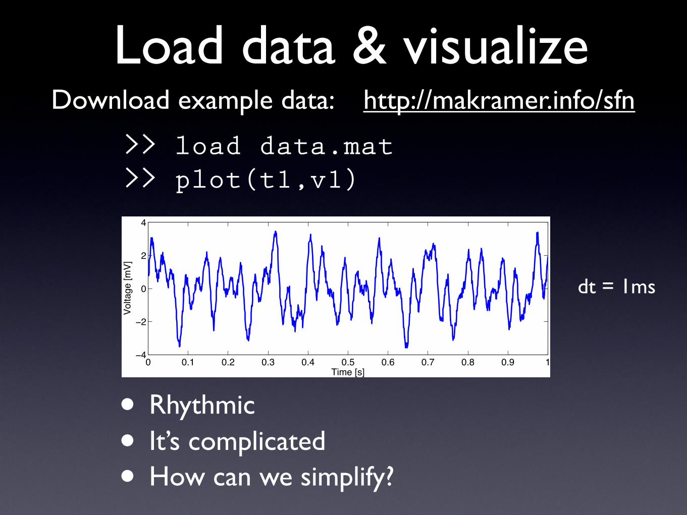
MATLAB code
Incomplete: Must label the x-axis?
0 100 200 300 400 500 600 700 800 900 1000−50
−40
−30
−20
−10
0
Indices []
Pow
er [d
B]
>> pow = (abs(fft(v1)).^2)/length(v1);>> pow = 10*log10(pow/max(pow));>> plot(pow)
http://makramer.info/sfn
Clue?
1000 data pts
Matcheslength of v1

0 100 200 300 400 500 600 700 800 900 1000−100
−80
−60
−40
−20
0
Indices []
Pow
er [d
B]
Power spectrum x-axis• Indices & frequencies related in a funny way . . .
Examine vector pow:
df2
2df3
fNQ - df500
fNQ
501-(fNQ - df)
502-3df998
-2df9991
f > 0 f < 0
• Because data is real, f < 0 is redundant.
... ...
Frequency resolution
Nyquistfrequency
Index
Freq1000
01000-df
What remains?
Find df and fNQ

• What is df?
1
V [f ] =
!!
"!
v[t]e2!iftdt (1)
P [f ] =|V [f ]|2
n(2)
df =1
T(3)where T = Total time of recording.
0 0.1 0.2 0.3 0.4 0.5 0.6 0.7 0.8 0.9 1−4
−2
0
2
4
Time [s]
Volta
ge [m
V]
Ex:T = 1 sdf = 1 Hz
Q: How do we improve frequency resolution?A: Increase T or record for longer time.
Power spectrum x-axis

Examples• Demand 0.2 Hz frequency resolution.
0 0.5 1 1.5 2 2.5 3 3.5 4 4.5 5!4
!2
0
2
4
6
Time [s]
Volta
ge []
But, data may change during longer recordings . . .
0 0.5 1 1.5 2 2.5 3 3.5 4 4.5 5!4
!2
0
2
4
Time [s]
Volta
ge []
Balance resolution requirements with consistency in data.
df = 1/5s = 0.2 Hz
Different spectra in 1st and 2nd half of data . . .

True signal: fs
• What is fNQ?
1
V [f ] =
!!
"!
v[t]e2!iftdt (1)
P [f ] =|V [f ]|2
n(2)
df =1
T(3)
fNQ =f0
2(4)The Nyquist frequency
where f0 = sampling frequency.
f0 >> 2 fs
The highest frequency we can observe.
f0 = 2 fs
f0 < 2 fs
Enough to reconstruct signal,
but just barely.
High frequency (in data) mapped to low frequency
(aliased).
Accurate reconstruction
Power spectrum x-axis
Too expensive!
Sample:
2 samples/cycleMax freq we can observe at this sample rate!
All hope lost! Indistinguishable from true low frequency signals.
0 0.1 0.2 0.3 0.4 0.5 0.6 0.7 0.8 0.9 1−4
−2
0
2
4
Time [s]
Volta
ge [m
V]
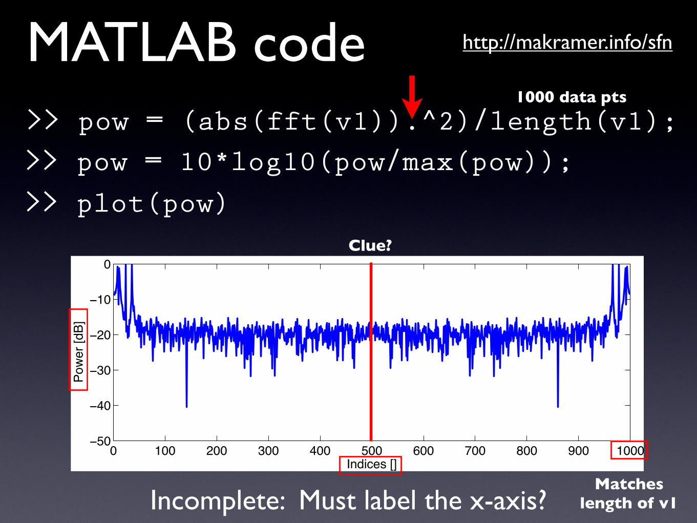
Ex:f0 = 1000 HzfNQ = 500 Hz
Q: How do we increase the Nyquist frequency?A: Increase the sampling rate f0. [Hardware]
Moral: Sample fast enough to capture the highest frequency “true” signal.
Power spectrum x-axis
dtSampling interval: Sampling frequency:= 1 msf0 = 1/dt

>> pow = (abs(fft(v1)).^2)/length(v1);
>> pow = 10*log10(pow/max(pow));
>> pow = pow(1:length(v1)/2+1);
0 5 10 15 20 25 30 35 40 45 50−50
−40
−30
−20
−10
0
Frequency [Hz]
Pow
er [d
B]
MATLAB code http://makramer.info/sfn
>> df = 1/max(t1); fNQ = 1/dt/2;
First half of data
>> faxis = (0:df:fNQ);Define df & fNQ
Frequency axis
>> plot(faxis, pow); xlim([0 50]);

Summary
• For finer frequency resolution: record more data.
• To observe higher frequencies: increase sampling rate.
>> pow = (abs(fft(v1)).^2)/length(v1);
• Many subtleties . . .
1
V [f ] =
!!
"!
v[t]e2!iftdt (1)
P [f ] =|V [f ]|2
n(2)
df =1
T(3)Frequency
resolution
1
V [f ] =
!!
"!
v[t]e2!iftdt (1)
P [f ] =|V [f ]|2
n(2)
df =1
T(3)
fNQ =f0
2(4)Nyquist
frequency
• Built-in routines: >> periodogram(...)Requires Signal Processing Toolbox
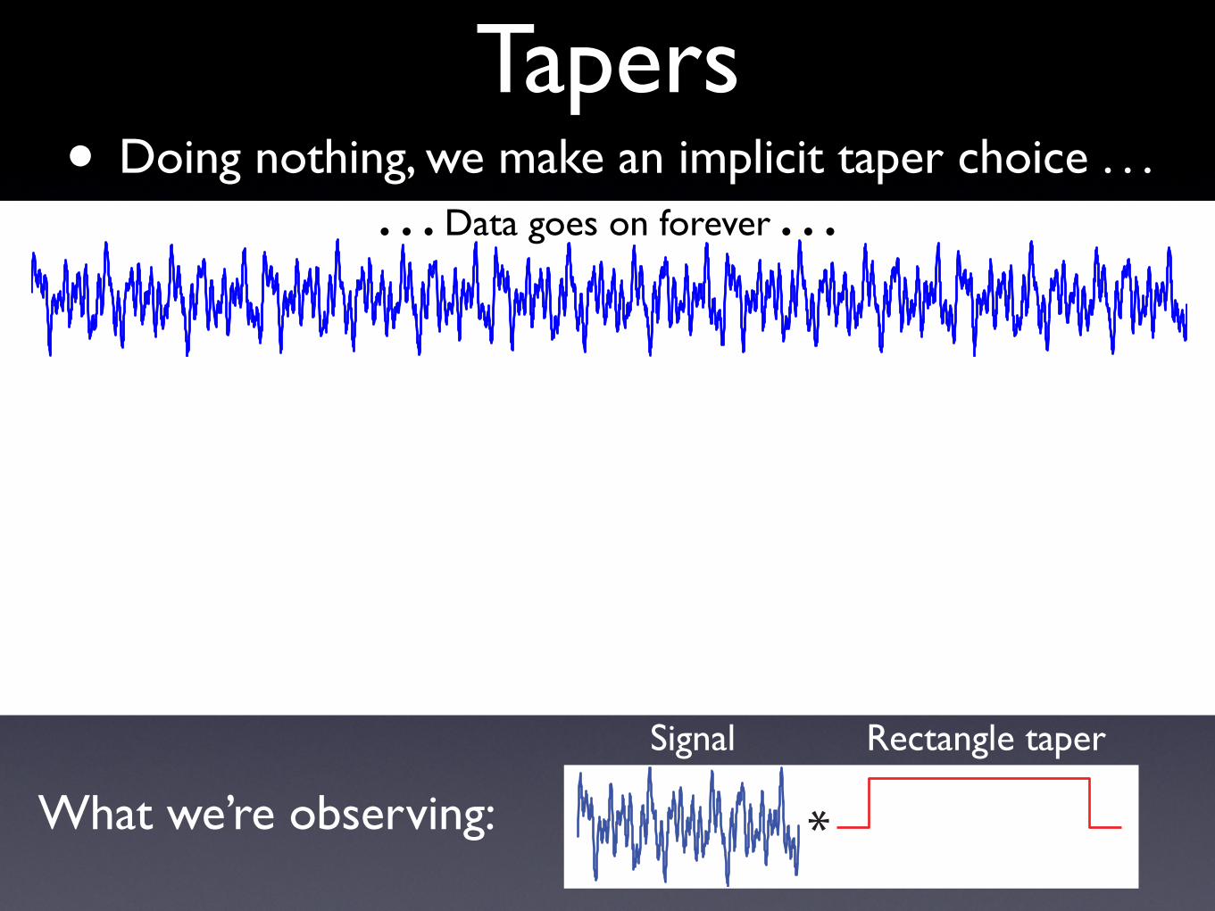
Tapers• Doing nothing, we make an implicit taper choice . . .
What we’re observing:
. . . Data goes on forever . . .
We we get:
0 0
But we observe it in a small window
0
1
Signal Rectangle taper
*

0 5 10 15 20 25 30 35 40
−30
−20
−10
0
Frequency [Hz]
Pow
er [d
B]
Spectrum we want
Tapers• The rectangle taper blurs the power spectrum.
0 5 10 15 20 25 30 35 40−40
−30
−20
−10
0
Frequency [Hz]
Pow
er [d
B]
What we get
Puresinusoid
0 0.1 0.2 0.3 0.4 0.5 0.6 0.7 0.8 0.9 1−1
−0.5
0
0.5
1
Time [s]
near 20 Hz 0 0.1 0.2 0.3 0.4 0.5 0.6 0.7 0.8 0.9 1−1
−0.5
0
0.5
1
Time [s]

Hann taper• Idea: smooth the sharp edges of rectangle taper.
>> st = s .* hann(length(s))’ ;
Taper reduces the “sidelobes”.
0 0.1 0.2 0.3 0.4 0.5 0.6 0.7 0.8 0.9 1−1
−0.5
0
0.5
1
Time [s]0 0.1 0.2 0.3 0.4 0.5 0.6 0.7 0.8 0.9 1
−1
−0.5
0
0.5
1
Time [s]
Hann Taper0 0.1 0.2 0.3 0.4 0.5 0.6 0.7 0.8 0.9 1
−1
−0.5
0
0.5
1
Time [s]
Data
Taper
0 5 10 15 20 25 30 35 40−40
−30
−20
−10
0
Frequency [Hz]
Pow
er [d
B]
Rect
0 5 10 15 20 25 30 35 40−40
−30
−20
−10
0
Frequency [Hz]
Pow
er [d
B]
RectHann
• Compute power spectrum of tapered data.Requires Signal Processing Toolbox

0 5 10 15 20 25 30 35 40 45 50−50−40−30−20−10
0
Frequency [Hz]
Pow
er [d
B]
Rect
0.1 0.2 0.3 0.4 0.5 0.6 0.7 0.8 0.9 1
−2
0
2
Time [s]
v1:
Ex: Hann taper
• Good: Deeper baseline• Bad: Broader peaks & lose data at edges.
0 0.1 0.2 0.3 0.4 0.5 0.6 0.7 0.8 0.9 1−1
−0.5
0
0.5
1
Time [s]
Lost Lost
0 5 10 15 20 25 30 35 40 45 50−50−40−30−20−10
0
Frequency [Hz]
Pow
er [d
B]
Rect
Hann

Multi-taper Method• Idea: Apply lots of different tapers
• Chronux (www.chronux.org)>> mtmspectrumc(v1,params);
0 5 10 15 20 25 30 35 40 45 50−60
−40
−20
0
Frequency [Hz]
Pow
er [d
B]
Reduce sidelobes
Keep data edges
0 0.1 0.2 0.3 0.4 0.5 0.6 0.7 0.8 0.9 1−0.06
−0.04
−0.02
0
0.02
0.04
0.06
Time [s]0 0.1 0.2 0.3 0.4 0.5 0.6 0.7 0.8 0.9 1
−0.06
−0.04
−0.02
0
0.02
0.04
0.06
Time [s]0 0.1 0.2 0.3 0.4 0.5 0.6 0.7 0.8 0.9 1
−0.06
−0.04
−0.02
0
0.02
0.04
0.06
Time [s]0 0.1 0.2 0.3 0.4 0.5 0.6 0.7 0.8 0.9 1
−0.06
−0.04
−0.02
0
0.02
0.04
0.06
Time [s]0 0.1 0.2 0.3 0.4 0.5 0.6 0.7 0.8 0.9 1
−0.06
−0.04
−0.02
0
0.02
0.04
0.06
Time [s]

Spectrogram
• Visual inspection• Data characteristics change in time.
• What if signal characteristics change in time?
0 1 2 3 4 5 6 7 8 9 10−2
−1
0
1
2
Time [s]
>> load data.mat>> plot(t2,v2) http://makramer.info/sfn

Spectrogram• Compute the spectrum (Hann taper) of all data
Q: Is this a good representation of the data?
0 5 10 15 20 25 30 35 40 45 50−60
−40
−20
0
Frequency [Hz]
Pow
er [d
B]
A: No, changing characteristics of the signal lost.
Time [s]
Freq
[Hz]
1 2 3 4 5 6 7 8 90
5
10
15
20
−40
−30
−20
−10
0

0 1 2 3 4 5 6 7 8 9 10−2
−1
0
1
2
Time [s]
Spectrogram• Idea: Split up the data into windows &
Compute spectrum in each.
df =
0 10 20 30 40 50−30
−20
−10
0
Frequency [Hz]
Pow
er [d
B]
0 10 20 30 40 50−30
−20
−10
0
Frequency [Hz]Po
wer
[dB]
Different spectra at beginning and end of signal.
1Hz
Repeat for many overlapping windows . . .

>> [S,F,T]=spectrogram(v2,1s,0.5s,1s,1kHz)
A better representation of the data?
Time [s]
Freq
[Hz]
1 2 3 4 5 6 7 8 90
5
10
15
20
−40
−30
−20
−10
0
MATLAB code http://makramer.info/sfnRequires Signal Processing Toolbox
Window
Overlap
Padding
f0
>> S = abs(S);
>> imagesc(T,F,10*log10(S/max(S(:))));
Plot power [color] vs frequency and time
Can compute multi-taper spectrogram! (Chronux)
Conclusions & Refs
• We focused on power spectrum (not wavelets).
• Defined df and fNQ.
• Explored tapers and spectrograms.
MATLAB for Neuroscientists, Numerical Recipes in C
Chronux.org and Neuroinformatics Summer Course
EEGLab
References

Coherence• Idea: examine phase relationship between signals.
• Requires two signals.
v3a v3b• Requires multiple trials for each signal.
10.1 0.2 0.3 0.4 0.5 0.6 0.7 0.8 0.9 1
−2
0
2
Time [s]0.1 0.2 0.3 0.4 0.5 0.6 0.7 0.8 0.9 1
−2
0
2
4
Time [s]
20.1 0.2 0.3 0.4 0.5 0.6 0.7 0.8 0.9 1
−4
−2
0
2
Time [s]0.1 0.2 0.3 0.4 0.5 0.6 0.7 0.8 0.9 1
−4
−2
0
2
Time [s]
30.1 0.2 0.3 0.4 0.5 0.6 0.7 0.8 0.9 1
−4
−2
0
2
4
Time [s]0.1 0.2 0.3 0.4 0.5 0.6 0.7 0.8 0.9 1
−2
0
2
Time [s]

>> load data.mat
Two variables: v3a & v3b
100Trials
1234
100
1000 indices1 ms 1000 ms
v3a0.1 0.2 0.3 0.4 0.5 0.6 0.7 0.8 0.9 1
−4
−2
0
2
Time [s]
0.1 0.2 0.3 0.4 0.5 0.6 0.7 0.8 0.9 1−4
−2
0
2
Time [s]
.
.
.
MATLAB code http://makramer.info/sfn

Power spectrum• Compute the power spectrum for each trial,
Then average over all trials.
Power at 10 Hz and 18 Hz.
Q: Are these rhythms coherent between v3a and v3b?
0 10 20 30 40 50−35
−30
−25
−20
−15
−10
−5
0
Frequency [Hz]
Pow
er [d
B]
v3a
0 10 20 30 40 50−35
−30
−25
−20
−15
−10
−5
0
Frequency [Hz]
Pow
er [d
B]
v3b

Coherence• For each trial, compute the phase at each frequency.
Re
Im
r
θ
= ( Re{V[f]}, Im{V[f]} )complex
Examine this complex plane for our data . . .
1
V [f ] =! !
"!v[t]e"2!iftdt (1)
P [f ] =|V [f ]|2
n(2)
df =1T
(3)
fNQ =f0
2(4)
C12[f ] =E{V1[f ]V #2 [f ]}
E{|V1[f ]|2}E{|V2[f ]|2} (5)
Fourier transform
Re{V[f]}
Im{V[f]} V[f]
θ = phase of V at frequency f.

2000
4000
6000
8000
30
210
60
240
90
270
120
300
150
330
180 0
v3a-v3b
Complex Plane at f =10 Hz
50
100
150
30
210
60
240
90
270
120
300
150
330
180 0
v3a
Complex Plane at f =10 Hz
Plot complex plane at 10 Hz• For each trial, compute FT(data) & plot . . .
Coherent at 10 Hz?
Phase concentration = Nonzero mean vector = coherent
Draw the vector to each complex difference.Compute the mean vector
Examine their difference (trial by trial).Summarize:
v3a[f]Trial 1
v3a[f]Trial 2v3a[f]
Trial 3
v3a[f]Trial 4
v3a[f]-v3b[f]Trial 1
v3a[f]-v3b[f]Trial 2
Get trail #1 data.Compute FTEvaluate at f=10 HzPlot it . . .
50
100
150
30
210
60
240
90
270
120
300
150
330
180 0
v3b
Complex Plane at f =10 Hz

100000
200000
300000
30
210
60
240
90
270
120
300
150
330
180 0
v3a-v3b
Complex Plane at f =18 Hz
Coherent? Plot the complex difference
Phase dispersion = Zero mean vector = No coherence
500
1000
30
210
60
240
90
270
120
300
150
330
180 0
v3a
Complex Plane at f =18 Hz
500
1000
30
210
60
240
90
270
120
300
150
330
180 0
v3b
Complex Plane at f =18 Hz
Draw the vector to each complex difference.Compute the mean vector
Summarize:
Plot complex plane at 18 Hz• For each trial, compute FT(data) & plot . . .

Coherence• Idea: Examine the “angular concentration” of
vector differences in the complex plane.
Strong power does not imply coherence.
0 10 20 30 40 50−35
−30
−25
−20
−15
−10
−5
0
Frequency [Hz]
Pow
er [d
B]
v3a
0 10 20 30 40 50−35
−30
−25
−20
−15
−10
−5
0
Frequency [Hz]
Pow
er [d
B]
v3b
0 10 20 30 40 500
0.2
0.4
0.6
0.8
1
Frequency [Hz]
Cohe
renc
e []
Coherentat 10 Hz
Not coherentat 18 Hz
Can compute multi-taper coherence! (Chronux)
18 Hz dominates 18 Hz dominates

Conclusions & Ref
• More about coherence:[Nunez et al., Electroenceph Clin Neurophys, 1997][Bruns, J Neurosci Methods, 2004]
• There are many coupling measuresCross correlation, phase consistency, Granger causality, cross-frequency coupling, . . .
[Pereda et al., Progress in Neurobiology (2005)]
• SfN AbstractsOnline:137 results for “coherence”.

Conclusions• We examined techniques to quantify
rhythms and their interactions in data.
• Many different techniques exist.
• Tutorial slides & MATLAB code availablehttp://makramer.info/sfn
• Contact me at SfN to talk more:Mark --- [email protected]
Thanks!

Extra Material

>> periodogram(v1,[],length(v1),1000Hz);
Signal Processing Toolbox
0 5 10 15 20 25 30 35 40 45 50−50
−40
−30
−20
−10
0
Frequency (Hz)
Pow
er/fr
eque
ncy
(dB/
Hz)
Periodogram Power Spectral Density Estimate
Taper Zero padding f0
•Use built-in MATLAB routine:
Correct axis!
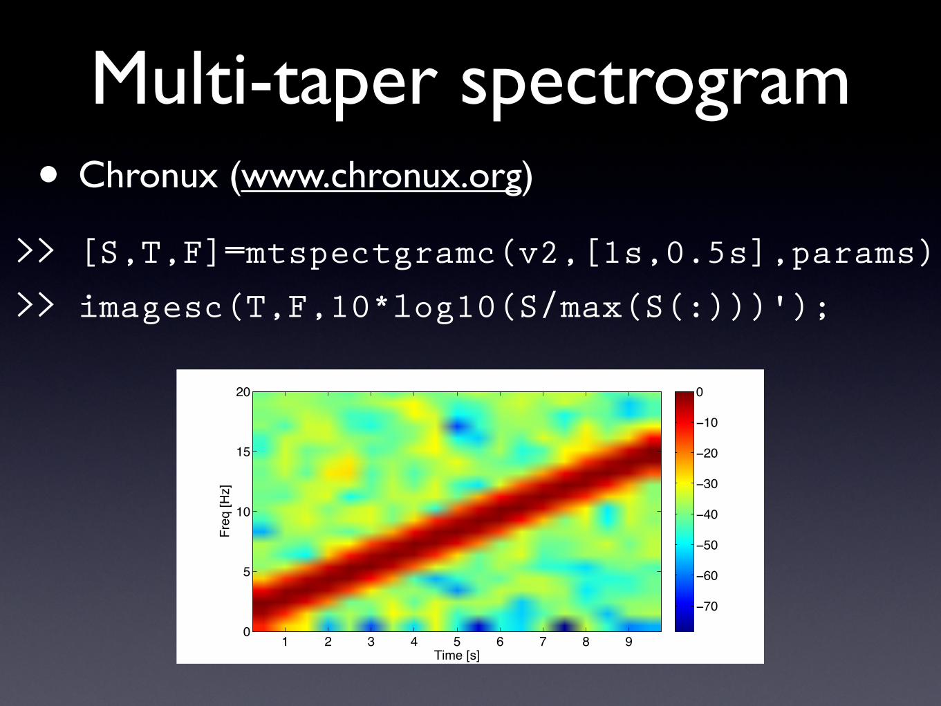
Multi-taper spectrogram
Time [s]
Freq
[Hz]
1 2 3 4 5 6 7 8 90
5
10
15
20
−70
−60
−50
−40
−30
−20
−10
0
>> [S,T,F]=mtspectgramc(v2,[1s,0.5s],params)
>> imagesc(T,F,10*log10(S/max(S(:)))');
• Chronux (www.chronux.org)

Multi-taper coherency
>> [C,phi,S12,S1,S2,f]=coherencyc(v3a',v3b',params)
>> plot(f,C);
• Chronux (www.chronux.org)
0 5 10 15 20 25 30 35 40 45 500
0.05
0.1
0.15
0.2
0.25
0.3
0.35
Frequency [Hz]
Cohe
renc
e []

Coherence formalism
1
V [f ] =! !
"!v[t]e2!iftdt (1)
P [f ] =|V [f ]|2
n(2)
df =1T
(3)
fNQ =f0
2(4)
C12[f ] =E{V1[f ]V #2 [f ]}
E{|V1[f ]|2}E{|V2[f ]|2} (5)E: Sum over trials
cross spectrum
power spectrum
Note: could taper here!
sxy = zeros(ntrials, ttrials);sxx = zeros(ntrials, ttrials);syy = zeros(ntrials, ttrials);
for k=1:ntrials sxy(k,:) = fft(v3a(k,:)).*conj(fft(v3b(k,:))); sxx(k,:) = fft(v3a(k,:)).*conj(fft(v3a(k,:))); syy(k,:) = fft(v3b(k,:)).*conj(fft(v3b(k,:)));end coh = (abs(sum(sxy,1)).^2) ./ (sum(sxx,1) .* sum(syy,1));plot(faxis, coh(1:length(coh)/2+1))xlim([0 50]); ylim([0 1])xlabel('Frequency [Hz]')ylabel('Coherence')
http://makramer.info/sfn
Define cross and power spectra
For each trail,compute spectra.
Sum over trials.