Analog vs. discrete signals - University of Waterlooece413/Sections/section1.pdf · Analog vs....

Analog vs. discrete signals

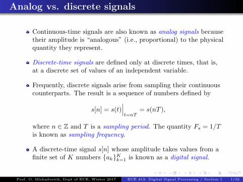
Continuous-time signals are also known as analog signals becausetheir amplitude is “analogous” (i.e., proportional) to the physicalquantity they represent.

Discrete-time signals are defined only at discrete times, that is,at a discrete set of values of an independent variable.

Frequently, discrete signals arise from sampling their continuouscounterparts. The result is a sequence of numbers defined by

s[n] = s(t)∣∣∣t=nT

= s(nT ),

where n ∈ Z and T is a sampling period. The quantity Fs = 1/Tis known as sampling frequency.

A discrete-time signal s[n] whose amplitude takes values from afinite set of K numbers {ak}Kk=1 is known as a digital signal.

Prof. O. Michailovich, Dept of ECE, Winter 2017 ECE 413: Digital Signal Processing / Section 1 1/32

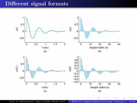
Different signal formats


Continuous-time systems

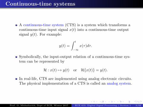
A continuous-time system (CTS) is a system which transforms acontinuous-time input signal x(t) into a continuous-time outputsignal y(t). For example:

y(t) =

∫ t

−∞x(τ)dτ.

Symbolically, the input-output relation of a continuous-time sys-tem can be represented by

H : x(t) 7→ y(t) or H{x(t)} = y(t).

In real-life, CTS are implemented using analog electronic circuits.The physical implementation of a CTS is called an analog system.


Discrete-time systems

A system that transforms a discrete-time input signal x[n] into adiscrete-time output signal y[n], is called a discrete-time system.

Symbolically, the input-output relation of a discrete-time systemis represented by

H : x[n] 7→ y[n] or H{x[n]} = y[n].

The physical implementation of discrete-time systems can be do-ne either in software or hardware.

In both cases, the underlying physical systems consist of digitalelectronic circuits designed to manipulate logical information orphysical quantities represented in digital form by binary electro-nic signals.


Analog-to-digital conversion

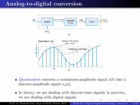
Quantization converts a continuous-amplitude signal x(t) into adiscrete-amplitude signal xd[n].

In theory, we are dealing with discrete-time signals; in practice,we are dealing with digital signals.


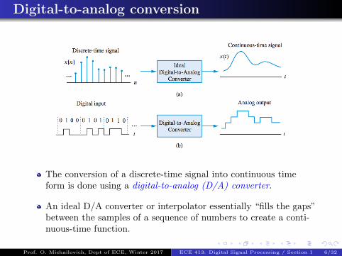
Digital-to-analog conversion

The conversion of a discrete-time signal into continuous timeform is done using a digital-to-analog (D/A) converter.

An ideal D/A converter or interpolator essentially “fills the gaps”between the samples of a sequence of numbers to create a conti-nuous-time function.


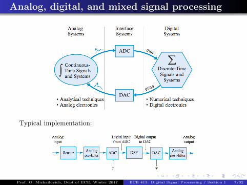
Analog, digital, and mixed signal processing

Typical implementation:


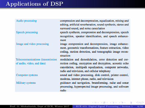
Applications of DSP


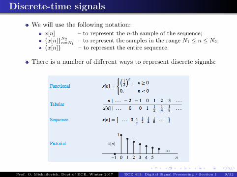
Discrete-time signals

We will use the following notation:

x[n] – to represent the n-th sample of the sequence;{x[n]}N2

n=N1– to represent the samples in the range N1 ≤ n ≤ N2;

{x[n]} – to represent the entire sequence.

There is a number of different ways to represent discrete signals:


Discrete-time signals (continued)

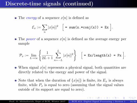
The energy of a sequence x[n] is defined as

Ex :=∑n

|x[n]|2[= sum(x.*conj(x)) = Ex

].

The power of a sequence x[n] is defined as the average energy persample

Px := limL→∞

{1

2L+ 1

L∑n=−L

|x[n]|2} [

= Ex/length(x) = Px].

When signal x[n] represents a physical signal, both quantities aredirectly related to the energy and power of the signal.

Note that when the duration of {x[n]} is finite, its Ex is alwaysfinite, while Px is equal to zero (assuming that the signal valuesoutside of its support are equal to zero).


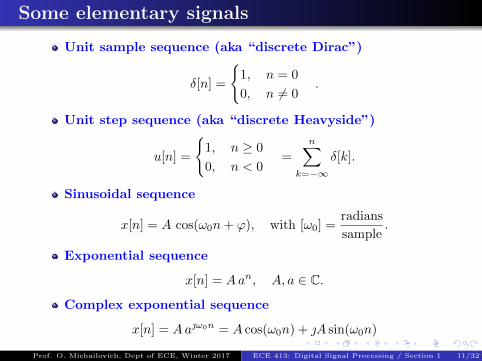
Some elementary signals

Unit sample sequence (aka “discrete Dirac”)

δ[n] =

{1, n = 0

0, n 6= 0.

Unit step sequence (aka “discrete Heavyside”)

u[n] =

{1, n ≥ 0

0, n < 0=

n∑k=−∞

δ[k].

Sinusoidal sequence

x[n] = A cos(ω0n+ ϕ), with [ω0] =radians

sample.

Exponential sequence

x[n] = Aan, A, a ∈ C.

Complex exponential sequence

x[n] = Aaω0n = A cos(ω0n) + A sin(ω0n)


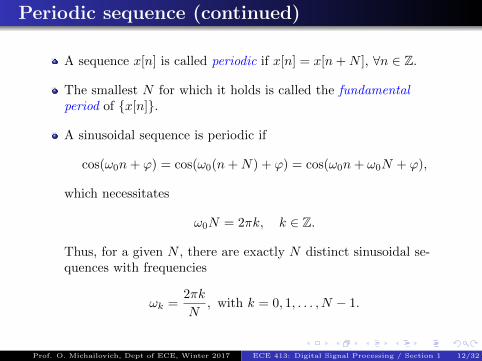
Periodic sequence (continued)

A sequence x[n] is called periodic if x[n] = x[n+N ], ∀n ∈ Z.

The smallest N for which it holds is called the fundamentalperiod of {x[n]}.

A sinusoidal sequence is periodic if

cos(ω0n+ ϕ) = cos(ω0(n+N) + ϕ) = cos(ω0n+ ω0N + ϕ),

which necessitates

ω0N = 2πk, k ∈ Z.

Thus, for a given N , there are exactly N distinct sinusoidal se-quences with frequencies

ωk =2πk

N, with k = 0, 1, . . . , N − 1.


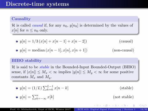
Discrete-time systems

Causality

H is called causal if, for any n0, y[n0] is determined by the values ofx[n] for n ≤ n0 only.

y[n] = 1/3 (x[n] + x[n− 1] + x[n− 2]) (causal)

y[n] = median (x[n− 1], x[n], x[n+ 1]) (non-causal)

BIBO stability

H is said to be stable in the Bounded-Input Bounded-Output (BIBO)sense, if |x[n]| ≤Mx <∞ implies |y[n]| ≤My <∞ for some positiveconstants Mx and My.

y[n] = (1/L)∑L−1

k=0 x[n− k] (stable)

y[n] =∑n

k=−∞ x[k] (not stable)


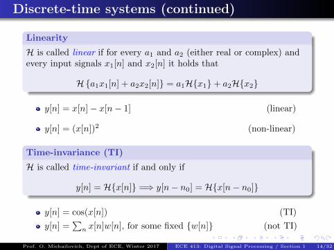
Discrete-time systems (continued)

Linearity

H is called linear if for every a1 and a2 (either real or complex) andevery input signals x1[n] and x2[n] it holds that

H{a1x1[n] + a2x2[n]} = a1H{x1}+ a2H{x2}

y[n] = x[n]− x[n− 1] (linear)

y[n] = (x[n])2 (non-linear)

Time-invariance (TI)

H is called time-invariant if and only if

y[n] = H{x[n]} =⇒ y[n− n0] = H{x[n− n0]}

y[n] = cos(x[n]) (TI)

y[n] =∑

n x[n]w[n], for some fixed {w[n]} (not TI)


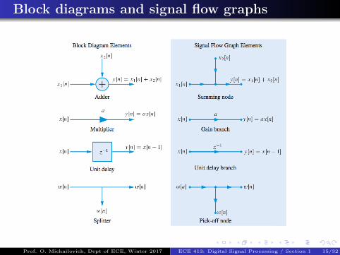
Block diagrams and signal flow graphs


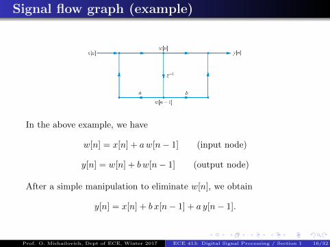
Signal flow graph (example)

In the above example, we have

w[n] = x[n] + aw[n− 1] (input node)

y[n] = w[n] + bw[n− 1] (output node)

After a simple manipulation to eliminate w[n], we obtain

y[n] = x[n] + b x[n− 1] + a y[n− 1].


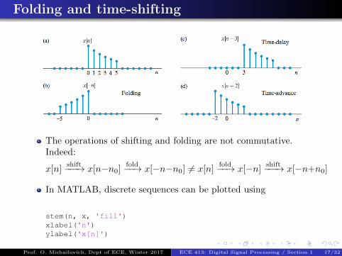
Folding and time-shifting

The operations of shifting and folding are not commutative.Indeed:

x[n]shift−−−→ x[n−n0]

fold−−→ x[−n−n0] 6= x[n]fold−−→ x[−n]

shift−−−→ x[−n+n0]

In MATLAB, discrete sequences can be plotted using

stem(n, x, 'fill')xlabel('n')ylabel('x[n]')


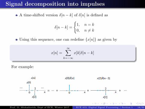
Signal decomposition into impulses

A time-shifted version δ[n− k] of δ[n] is defined as

δ[n− k] =

{1, n = k

0, n 6= k

Using this sequence, one can redefine {x[n]} as given by

x[n] =

∞∑k=−∞

x[k]δ[n− k]

For example:


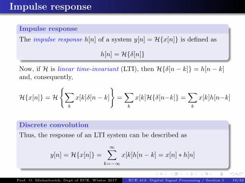
Impulse response

Impulse response

The impulse response h[n] of a system y[n] = H{x[n]} is defined as

h[n] = H{δ[n]}

Now, if H is linear time-invariant (LTI), then H{δ[n− k]} = h[n− k]and, consequently,

H{x[n]} = H

{∑k

x[k]δ[n− k]

}=∑k

x[k]H{δ[n−k]} =∑k

x[k]h[n−k]

Discrete convolution

Thus, the response of an LTI system can be described as

y[n] = H{x[n]} =

∞∑k=−∞

x[k]h[n− k] = x[n] ∗ h[n]


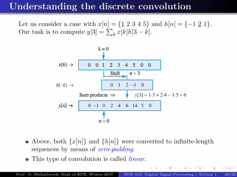
Understanding the discrete convolution

Let us consider a case with x[n] = {1 2 3 4 5} and h[n] = {−1 2 1}.Our task is to compute y[3] =

∑k x[k]h[3− k].

Above, both {x[n]} and {h[n]} were converted to infinite-lengthsequences by means of zero-padding.

This type of convolution is called linear.


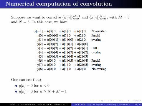
Numerical computation of convolution

Suppose we want to convolve {h[n]}M−1n=0 and {x[n]}N−1n=0 , with M = 3and N = 6. In this case, we have

One can see that:

y[n] = 0 for n < 0

y[n] = 0 for n ≥ N +M − 1


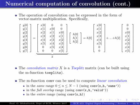
Numerical computation of convolution (cont.)

The operation of convolution can be expressed in the form ofvector-matrix multiplication. Specifically,

y[0]y[1]y[2]y[3]y[4]y[5]y[6]y[7]

=

x[0] 0 0x[1] x[0] 0x[2] x[1] x[0]x[3] x[2] x[1]x[4] x[3] x[2]x[5] x[4] x[3]0 x[5] x[4]0 0 x[5]

︸︷︷︸

X

h[0]h[1]h[2]

= h[0]

x[0]x[1]x[2]x[3]x[4]x[5]00

+. . .+h[2]

00

x[0]x[1]x[2]x[3]x[4]x[5]

The convolution matrix X is a Toeplitz matrix (can be built usingthe m-function toeplitz).

The m-function conv can be used to compute linear convolution

in the same range 0 ≤ n ≤ N − 1 (using conv(x,h,’same’))in the full overlap range (using conv(x,h,’valid’))in the entire range (using conv(x,h))


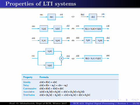
Properties of LTI systems


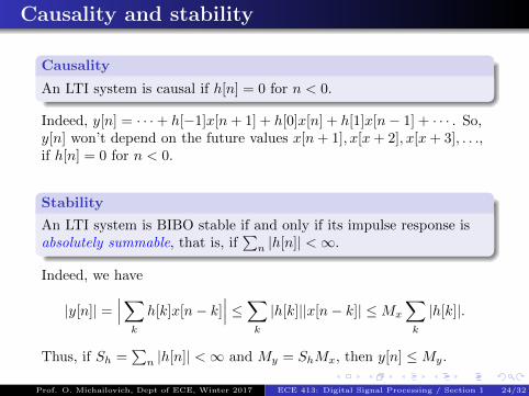
Causality and stability

Causality

An LTI system is causal if h[n] = 0 for n < 0.

Indeed, y[n] = · · ·+ h[−1]x[n+ 1] + h[0]x[n] + h[1]x[n− 1] + · · · . So,y[n] won’t depend on the future values x[n+ 1], x[x+ 2], x[x+ 3], . . .,if h[n] = 0 for n < 0.

Stability

An LTI system is BIBO stable if and only if its impulse response isabsolutely summable, that is, if

∑n |h[n]| <∞.

Indeed, we have

|y[n]| =∣∣∣∑

k

h[k]x[n− k]∣∣∣ ≤∑

k

|h[k]||x[n− k]| ≤Mx

∑k

|h[k]|.

Thus, if Sh =∑

n |h[n]| <∞ and My = ShMx, then y[n] ≤My.


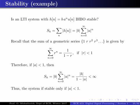
Stability (example)

Is an LTI system with h[n] = b anu[n] BIBO stable?

Sh =∑n

|h[n]| = |b|∞∑

n=0

|a|n

Recall that the sum of a geometric series {1 r r2 r3 . . .} is given by

∞∑n=0

rn =1

1− r, if |r| < 1

Therefore, if |a| < 1, then

Sh = |b|∞∑

n=0

|a|n =|b|

1− |a|<∞

Thus, the system if stable only if |a| < 1.


Recursive implementation of LTI systems

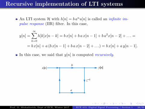
An LTI system H with h[n] = b anu[n] is called an infinite im-pulse response (IIR) filter. In this case,

y[n] =

∞∑k=0

h[k]x[n− k] = b x[n] + b a x[n− 1] + b a2x[n− 2] + . . . =

= b x[n] + a (b x[n− 1] + b a x[n− 2] + . . .) = b x[n] + a y[n− 1].

In this case, we said that y[n] is computed recursively.


Linear constant coefficients difference equations

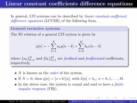
In general, LTI systems can be described by linear constant-coefficientdifference equations (LCCDE) of the following form.

General recursive systems

The IO relation of a general LTI system is given by

y[n] = −N∑

k=1

aky[n− k] +

M∑k=0

bkx[n− k]

where {ak}Nk=1 and {bk}Mk=1 are feedback and feedforward coefficients,respectively.

N is known as the order of the system.

If N = 0, then y[n] = (x ∗ h)[n], with h[n] = bn, n = 0, 1, . . . ,M .

In the above case, the system is causal and said to have a finiteimpulse response (FIR).


Real-time implementation of FIR filters

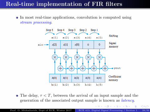
In most real-time applications, convolution is computed usingstream processing.

The delay, τ < T , between the arrival of an input sample and thegeneration of the associated output sample is known as latency.


Recursive FIR systems

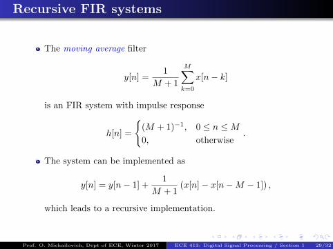
The moving average filter

y[n] =1

M + 1

M∑k=0

x[n− k]

is an FIR system with impulse response

h[n] =

{(M + 1)−1, 0 ≤ n ≤M0, otherwise

.

The system can be implemented as

y[n] = y[n− 1] +1

M + 1(x[n]− x[n−M − 1]) ,

which leads to a recursive implementation.


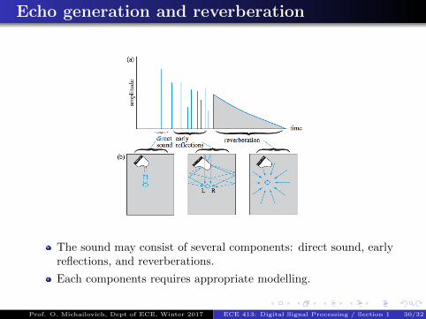
Echo generation and reverberation

The sound may consist of several components: direct sound, earlyreflections, and reverberations.

Each components requires appropriate modelling.


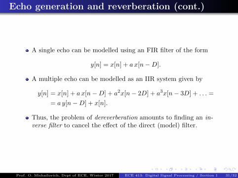
Echo generation and reverberation (cont.)

A single echo can be modelled using an FIR filter of the form

y[n] = x[n] + a x[n−D].

A multiple echo can be modelled as an IIR system given by

y[n] = x[n] + a x[n−D] + a2x[n− 2D] + a3x[n− 3D] + . . . =

= a y[n−D] + x[n].

Thus, the problem of dereverberation amounts to finding an in-verse filter to cancel the effect of the direct (model) filter.


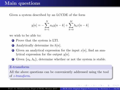
Main questions

Given a system described by an LCCDE of the form

y[n] = −N∑

k=1

aky[n− k] +

M∑k=0

bkx[n− k]

we wish to be able to:

1 Prove that the system is LTI.

2 Analytically determine its h[n].

3 Given an analytical expression for the input x[n], find an ana-lytical expression for the output y[n].

4 Given {ak, bk}, determine whether or not the system is stable.

Z-transform

All the above questions can be conveniently addressed using the toolof z-transform.


Analog vs. discrete signals - University of Waterlooece413/Sections/section1.pdf · Analog vs....

Documents

Transcript of Analog vs. discrete signals - University of Waterlooece413/Sections/section1.pdf · Analog vs....