
Design Techniques for Approximation Algorithms and Approximation Classes.
date post
20-Dec-2015Category
view
249download
4
Analog Filters: The Approximation
Franco Maloberti

Franco Maloberti Analog Filters: The Approximation
2
Introduction
The first step of the normalized filter design is to find a magnitude characteristics, |H(j)|, that fulfills the specifications
Handling |H(j)| it is difficult. It is better to deal with |H(j)|2.
|H(j)|2 is a rationale function in 2
€
H( jω)2
= H(s)H(−s)s= jω
= H( jω)H*( jω)

Franco Maloberti Analog Filters: The Approximation
3
Example
Consider the transfer function
€
H(s) =s+ 2
s3 + 2s2 + 2s+ 3
H(s)H(−s) =(s+ 2)(−s+ 2)
(s3 + 2s2 + 2s+ 3)(−s3 + 2s2 − 2s+ 3)=
−s2 + 4
−s6 + 8s2 + 9
H( jω)2
=ω2 + 4
ω6 − 8ω2 + 9
€
H( jω)2
=ω2 + 4
ω6 − 8ω2 + 9
Much easier to deal than

Franco Maloberti Analog Filters: The Approximation
4
Methodology
The approximation phase is based on the following: Find a real rationale function in 2 capable to
met the magnitude specifications (pass-band and stop-band)
Live with the resulting phase response Correct (if necessary) the phase response (or
delay) with a cascaded network Work on low-pass characteristics (we will se
shortly how to achieve high-pass, band-pass, … from a low-pass TF)

Franco Maloberti Analog Filters: The Approximation
5
Generic Low-Pass TF
A generic form of a low-pass TF is:
€
H( jω)2
=A0
1+ F(ω2)
F(ω2) <<1 for 0 ≤ω ≤ωp
F(ω2) >>1 for ω >>ωp
In the pass-band H()=A0
p
A0

Franco Maloberti Analog Filters: The Approximation
6
Butterworth Characteristics
A very simple form for F(2) is
n is the order of the Butterworth filter Properties:€
F(ω2) =ω2n
H( jω)2
=A0
1+ω2n
€
H( jω)Max
= H( j0) =1
H( j1) =1
2 (−3 dB or half − power)

Franco Maloberti Analog Filters: The Approximation
7
Maximally Flat
The magnitude response of the Butterworth filter is said to be maximally flat.
If we take the first 2n-1 derivatives of H(j), they are all zero at =0
€
H( jω) = (1+ω2n )−1/2
0 10 20 30 40 50 60 70 80 90 1000
0.1
0.2
0.3
0.4
0.5
0.6
0.7
0.8
0.9
1
n=8
=0,…,2

Franco Maloberti Analog Filters: The Approximation
8
0 0.2 0.4 0.6 0.8 1 1.2 1.4 1.6 1.8 20
0.1
0.2
0.3
0.4
0.5
0.6
0.7
0.8
0.9
1
Butterworth Plots; |H(j)|2
clear all;omega=linspace(0,2,100);for k=1:6n=k;for i=1:100Butter(i,k)=1/(1+omega(i)^(2*n));endendplot(omega,Butter);
All curves cross 0.5For =1

Franco Maloberti Analog Filters: The Approximation
9
Butterworth Plots
For >>1 |H(i)|2 ≈ 1/(2n) H(j)|dB = -20 n log
clear all;omega=linspace(0,100,100);for k=1:4n=k;for i=1:100Butter(i,k)=1/(1+omega(i)^(2*n));ButdB(i,k) = 20* log10(Butter(i,k));endendsemilogx(omega,ButdB);

Franco Maloberti Analog Filters: The Approximation
10
Design of Butterworth filters
Specifications
€
α s =10log(1+ωs2n )
α p =10log(1+ωp2n )
ωs2n =10α s /10 −1
ωp2n =10α p /10 −1
ωsωp
⎛
⎝ ⎜ ⎜
⎞
⎠ ⎟ ⎟
2n
=10α s /10 −1
10α p /10 −1
The values of αs, αp and the ratio s/p determine the ordern of the filter.
dB|H(j)|2pαssαp

Franco Maloberti Analog Filters: The Approximation
11
Chebyshev Characteristics
The Chebishev filters are based on the Chebishev polynomials
n is the order It is a polynomial!
€
Cn (ω) = cos(ncos−1ω)
€
cosθ =ω θ = cos−1ω
Cn (ω) = cos(nθ)

Franco Maloberti Analog Filters: The Approximation
12
Chebyshev Polynomials
€
Cn (ω) = cos(nθ)
Cn+1(ω) = cos(nθ +θ) = cosnθ cosθ − sinnθ sinθ
Cn−1(ω) = cos(nθ −θ) = cosnθ cosθ + sinnθ sinθ
Cn+1(ω) +Cn−1(ω) = 2cosnθ cosθ
Cn (ω) ω
Cn+1(ω) = 2ωCn (ω) −Cn−1(ω)

Franco Maloberti Analog Filters: The Approximation
13
Chebyshev Polynomials
€
C0(ω) = cos0 =1
C1(ω) = cos(cos−1ω) =ω
C2(ω) = 2ω2 −1
C3(ω) = 2(2ω2 −1)ω −ω = 4ω3 − 3ω
C4 (ω) = 2(4ω3 − 3ω)ω − (2ω2 −1) = 8ω4 − 8ω2 +1
€
Cn (ω) = 2n−1ωn +K

Franco Maloberti Analog Filters: The Approximation
14
-1.5 -1 -0.5 0 0.5 1 1.5-15
-10
-5
0
5
10
15
Chebyshev Polynomials Features
If varies in the range -1 +1 Cn()=cos(n+) limited to the range -1 +1
If | | is larger than 1 Cn()=cosh(n cosh-1 ) increases monotonically
with n.
clear all;n=7xmax=1+5/n^2;w=linspace(-xmax,xmax,200);for i=1:200C(i)=cos(n*acos(w(i)));endplot(w,C);

Franco Maloberti Analog Filters: The Approximation
15
Chebyshev low-pass
Choose a small number and let
the low-pass transfer function is
Normalize p = 1 Maximum attenuation in the pass-band
€
F(ω2) = ε 2Cn2(ω)
€
H( jω)2
=1
1+ ε 2Cn2(ω)
€
H( jω)min
2=
1
1+ ε 2
α s =10log(1+ ε 2)

Franco Maloberti Analog Filters: The Approximation
16
Chebyshev low-pass Plots
clear all;n = input('what is the order? ');eps = input('what is the value of epsilon? ');xmax=2;w=linspace(0,xmax,200);for i=1:200
C(i)=cos(n*acos(w(i)));H(i)=1/(1+(eps*C(i))^2);
endplot(w,H);
0 0.2 0.4 0.6 0.8 1 1.2 1.4 1.6 1.8 20
0.1
0.2
0.3
0.4
0.5
0.6
0.7
0.8
0.9
1
Order 4Eps=0.4
0 0.2 0.4 0.6 0.8 1 1.2 1.4 1.6 1.8 20
0.1
0.2
0.3
0.4
0.5
0.6
0.7
0.8
0.9
1
Order 7Eps=0.2

Franco Maloberti Analog Filters: The Approximation
17
Start from specifications
Determine
The order of the filter must be such that
Remember that
Chebyshev Filter DesigndB|H(j)|2pαssαp
€
α p =10log(1+ ε 2)
€
= 10α p /10 −1
€
α s =10log[1+ ε 2Cn2(ωs /ωp ))]
€
Cn (ωs /ωp ) = cosh(cosh−1(ωs /ωp ))
n =cosh−1[Cn (ωs /ωp )]
cosh−1(ωs /ωp )

Franco Maloberti Analog Filters: The Approximation
18
Other Chebyshev Responses
Define another function
Use in the Matlab program
€
Ha ( jω)2
=1− H( jω)2
0 0.2 0.4 0.6 0.8 1 1.2 1.4 1.6 1.8 20
0.1
0.2
0.3
0.4
0.5
0.6
0.7
0.8
0.9
1
0 0.2 0.4 0.6 0.8 1 1.2 1.4 1.6 1.8 20
0.1
0.2
0.3
0.4
0.5
0.6
0.7
0.8
0.9
1
H(i)=1-1/(1+(eps*C(i))^2);

Franco Maloberti Analog Filters: The Approximation
19
Inverse Chebyshev High-pass
0 0.2 0.4 0.6 0.8 1 1.2 1.4 1.6 1.8 20
0.1
0.2
0.3
0.4
0.5
0.6
0.7
0.8
0.9
1
€
Hb ( jω)2
=1
1+ ε 2Cn2(1 /ω)
clear all;n = input('what is the order? ');eps = input('what is epsilon? ');xmax=2;w=linspace(0,xmax,200);for i=1:200
C(i)=cos(n*acos((1/w(i))));H(i)=1/(1+(eps*C(i))^2);
endplot(w,H);
Franco Maloberti Analog Filters: The Approximation
20
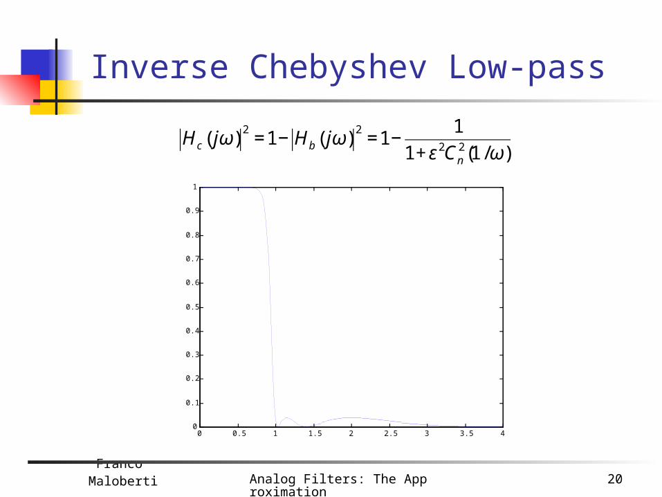
Inverse Chebyshev Low-pass
€
Hc ( jω)2
=1− Hb ( jω)2
=1−1
1+ ε 2Cn2(1 /ω)
0 0.5 1 1.5 2 2.5 3 3.5 40
0.1
0.2
0.3
0.4
0.5
0.6
0.7
0.8
0.9
1

Franco Maloberti Analog Filters: The Approximation
21
Elliptic-Function
Butterworth and Chebyshev don’t have finite zeros All-pole functions
Finite zeros help in the pass-band stop-band transition (see inverse Chebyshev)
Elliptic functions are a special category of zero-pole transfer functions
€
Hc ( jω)2
=P( jω)
2
Q( jω)2

Franco Maloberti Analog Filters: The Approximation
22
Elliptic-Function (ii)
Define RN()
or
Poles and zeros are reciprocal of one another If 1, 2,… are in the range 0 ≤ ≤1 |R()|2 is
zero at 1, 2,… and infinite at 1/1, 1/2,…
€
RN (ω) =(ω1
2 −ω2)(ω22 −ω2)L (ωN
2 −ω2)
(1−ω12ω2)(1−ω2
2ω2)L (1−ωN2ω2)
€
RN (ω) =ω(ω1
2 −ω2)(ω22 −ω2)L (ωN
2 −ω2)
(1−ω12ω2)(1−ω2
2ω2)L (1−ωN2ω2)

Franco Maloberti Analog Filters: The Approximation
23
Elliptic-Function (iii)
The elliptic characteristics is
€
H( jω)2
=1
1+ ε 2RN2 (ω)

Franco Maloberti Analog Filters: The Approximation
24
Plot of the Elliptic Function
clear all;n=5;eps=8;xmax=0.91;om1sq=0.1;om2sq=0.4;om3sq=0.65;om4sq=0.8;omega=linspace(0,xmax,200);for i=1:200w=omega(i);Num=w*(om1sq-w*w)*(om2sq-w*w)*(om3sq-w*w)*(om4sq-w*w);Den=(1-om1sq*w*w)*(1-om2sq*w*w)*(1-om3sq*w*w)*(1-om4sq*w*w);R(i)=Num/Den;Ellip(i)=1/(1+(eps*R(i))^2);endplot(omega,Ellip);
0 0.1 0.2 0.3 0.4 0.5 0.6 0.7 0.8 0.90.996
0.9965
0.997
0.9975
0.998
0.9985
0.999
0.9995
1
1.0005
1.1 1.2 1.3 1.4 1.5 1.6 1.7 1.8 1.9 20
0.5
1
1.5
2
2.5
3x 10⁻⁶
Pass
Stop

Franco Maloberti Analog Filters: The Approximation
25
Determine the order of a Filter
BUTTORD Butterworth filter order selection. [N, Wn] = BUTTORD(Wp, Ws, Rp, Rs) returns the order N of the lowest order digital Butterworth filter that loses no more than Rp dB in the passband and has at least Rs dB of attenuation in the stopband. Wp and Ws are the passband and stopband edge frequencies, normalized from 0 to 1 (where 1 corresponds to pi radians). For example, Lowpass: Wp = .1, Ws = .2 Highpass: Wp = .2, Ws = .1 Bandpass: Wp = [.1 .8], Ws = [.2 .7] Bandstop: Wp = [.2 .7], Ws = [.1 .8] BUTTORD also returns Wn, the Butterworth natural frequency (or, the "3 dB frequency") to use with BUTTER to achieve the specifications. [N, Wn] = BUTTORD(Wp, Ws, Rp, Rs, 's') does the computation for an analog filter, in which case Wp and Ws are in radians/second.
»help buttord
Franco Maloberti Analog Filters: The Approximation
26
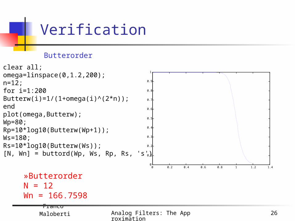
Verification
»ButterorderN = 12Wn = 166.7598
0 0.2 0.4 0.6 0.8 1 1.2 1.40
0.1
0.2
0.3
0.4
0.5
0.6
0.7
0.8
0.9
1clear all;omega=linspace(0,1.2,200);n=12;for i=1:200Butterw(i)=1/(1+omega(i)^(2*n));endplot(omega,Butterw);Wp=80;Rp=10*log10(Butterw(Wp+1));Ws=180;Rs=10*log10(Butterw(Ws));[N, Wn] = buttord(Wp, Ws, Rp, Rs, 's')
Butterorder

Franco Maloberti Analog Filters: The Approximation
27
Order of Chebishev or Elliptic filters
[N, Wn] = CHEB1ORD(Wp, Ws, Rp, Rs, 's') does the computation for an analog filter, in which case Wp and Ws are in radians/second.
[N, Wn] = ELLIPORD(Wp, Ws, Rp, Rs, 's') does the computation for an analog filter, in which case Wp and Ws are in radians/second.
clear all;Wp=2*pi;k=input('normalized stop frequency ')Ws=k*Wp;Rp=input('attenuation passband ')Rs=input('attenuation stopband ')[Nbutter, Wn] = BUTTORD (Wp, Ws, Rp, Rs, 's')[NCheb1, Wn] = CHEB1ORD(Wp, Ws, Rp, Rs, 's')[Nellip, Wn] = ELLIPORD(Wp, Ws, Rp, Rs, 's')
Comparing the orders »OrderFilternormalized stop frequency 1.2attenuation passband 0.2attenuation stopband 25
Nbutter = 25Wn = 6.7203NCheb1 = 9Wn = 6.2832Nellip = 5Wn = 6.2832

Franco Maloberti Analog Filters: The Approximation
28
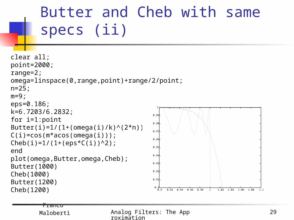
Butter and Cheb with same specs
stop frequency 1.2attenuation PB 0.2 dBattenuation SB 25 dB
Nbutter = 25Wn = 6.7203NCheb1 = 9Wn = 6.2832
0 0.5 1 1.5 2 2.50
0.1
0.2
0.3
0.4
0.5
0.6
0.7
0.8
0.9
1
Franco Maloberti Analog Filters: The Approximation
29
Butter and Cheb with same specs (ii)
clear all;point=2000;range=2;omega=linspace(0,range,point)+range/2/point;n=25;m=9;eps=0.186;k=6.7203/6.2832;for i=1:pointButter(i)=1/(1+(omega(i)/k)^(2*n));C(i)=cos(m*acos(omega(i)));Cheb(i)=1/(1+(eps*C(i))^2);endplot(omega,Butter,omega,Cheb);Butter(1000)Cheb(1000)Butter(1200)Cheb(1200)