XLVIII Reunión AnualNoviembre de 2013

ISSN 1852-0022ISBN 978-987-28590-1-5

AN ESSAY ON LONG-TERM CYCLICAL OSCILLATIONS OF ADVANCED EUROPEAN COUNTRIES AND THE US ECONOMY (1993-2012)

Baccino Osvaldo

ANALES | ASOCIACION ARGENTINA DE ECONOMIA POLITICA

“An Essay on Long-term Cyclical Oscillations of Advanced European Countries and the US Economy (1993q1-2012q3)” by Osvaldo E. Baccino The aim of this paper is to detect some kind of relationship between long-term oscillations of some advanced European economies and equivalent cyclicities in the American economy. The idea consists in identifying some leads and lags existing between the economic activity and investment of pairs of countries for some periodic trajectories. Nonetheless, it is important to have in mind that the study, at this stage, does not intend to measure the business cycle in the countries included in the sample, but to focus on some characteristics of periodic movements in a given range of frequency. No doubt, the result of this analysis may be helpful for a study of the business cycle of the considered countries but this is outside the reach of the present paper. The present task concentrates on the evolution of GDP and gross fixed investment to determine the most relevant long-term-oscillations taking place, and to relate those characteristics with those existing in the USA economy. The work develops particularly in the dominion of frequency of the study of time series. So that, a time series can be understood as a sum of sine waves, each with different cycle length, amplitudes and phases. Therefore, the spectral analysis allows detecting the most relevant cyclicities in the time series, and with that information it is possible to estimate their cyclical behaviour. Since this study is concerned about long swing movements, the shorter oscillations must be out of the analysis. For that reason, the seasonally adjusted time series were chosen. The search for long-run oscillations rests on the fact that the present world crisis is very big. Here, there is no assumption that the present world depression belongs to a definite cycle that links the 1930’s depression with the present one. Then, it is likely that such an extremely long cycle, definitely does not exist. Rather, these two deep depressions may be independent of each other. If this is the case, it is also likely that the way out of the present crisis may be through a particular long-term-cycle that is normal for most economies. Then the twenty-year long cycle seems an adequate choice as a relevant long-term behaviour. The data were collected from the OECD website (see References at the end of the paper); they were the quarterly gross domestic product and gross capital formation, both expressed in volume indexes seasonally adjusted. Besides, chain indices are good for calculating volume changes, though the resulting chained volume estimates are not additive. The series were de-trended by linear regression before calculating the periodograms. The Analysis of the Time Series The technique mainly used in this study is the spectral analysis of time series. In other words, this means that the study is performed in the dominion of the frequency, instead of the time-domain where the measurements are made against time. In the frequency-dominion, a time series is represented as a sum of sine waves, each with different amplitudes and phases, and corresponding to a given frequency. Many of

2

these oscillations cannot be detected by the naked eye. Therefore, to identify these oscillations, one has to make a spectral decomposition of the time series, and evaluate the degree of importance of those cyclicities. The analytical tool that expresses the spectral density associated with a range of frequencies is the periodogram and the spectrum of the time series. The spectrum derives from an initial estimation of the Periodogram, invented by Sir Arthur Schuster in 1898 that can be described by the following formula:

∑−

=+∑

−

==

21

0

2sin

21

0

2cos2

1)(

T

t

fttxT

t

fttxT

fI πππ

(1)

Where I(f) is the periodogram as a function of the frequency f, T is the number of observations of the time series xt. and t is the time variable. The periodogram measures the variance of the de-trended series associated with each frequency. Here both each periodogram and cross periodogram were computed by the fast Fourier transform, ds(f), where the subscript denotes the variable.

∑−

=

−=1

0

21)(

T

t

iftetsT

fsd π (2)

T

fdfdxxP xx

π2

)()(= and T

fxdfydyxP

π2

)()(= (3)

The bar expresses the complex conjugate, and i is the complex imaginary part of the number. However, owing to limitations of the periodograms it is necessary to smooth it to reach a more precise estimate of the spectral density function, The result is called the spectrum S(f). The data used in this study correspond to the series of gross domestic product (volume index) and gross capital formation (volume index) for Germany, France, UK, Italy and USA. The period covers from 1993q1 to 2012q3, that is 79 observations. The chosen time series were seasonally adjusted and this meant that short-term oscillations had been filtered. So that, spectral density will present only the long-term cyclicities as needed in the present study. A modified Daniell filter with five weigths was applied to smooth the periodograms previously obtained.1

∑−=

++−+−−

=1

1)2(

2

1)()2(

2

1

1

1

jffxxPjffxxPffxxP

mxxSD (4)

1 The first and last observations of the periodogram series maintain their value in the Spectrum. The second and the one before the last apply a three weight moving average such as [0.25, 0.50, 0.25]. The rest of the data uses the five weight formula depicted above.

3

With m = 5 the weigths are 0.125, 0.25, 0.25, 0.25 and 0.125. The symbol SDXX denotes Spectrum obtained with the Daniell’s filter, and PXX is the periodogram. The Daniell’s window allows constructing each ordinate of the spectrum by averaging the periodogram in the field determined by the window. The window has five components whose weighted average applies to the central component. Each frequency corresponds to the overtones of the fundamental frequency 1/79. The treatment followed in this paper about the spectral analysis of the GDP and Gross Capital Formation in volume indexes consists of three parts:

(i) There is a direct comparison of spectral density function among countries (ii) Then, it is performed a bivariate analysis for both variables between each

European Country and the USA’s economy. The aim of this analysis is to work with the joint structure of a pair of variables and identify the dependence of either series on the other.

(iii) A bivariate analysis was extended to the relationship between gross capital formation and gross domestic product for each country. In this part, the stress is placed upon the dependence of economic activity on fixed investment. There are a lot of dynamic components in a given time series and they do not follow a unique pattern of behaviour with all the components. The economic behaviour has differences according to the stretch of time at which it is considered. In analogous manner, the ordinates of the periodogram are quite independent one of the other. Therefore, one must expect that the direction of dependence between two countries, if it exists, is not uniform irrespective of the frequency of the oscillation. Those interconnections cannot be seen at first glance, since they are obscured by the superposition of other components of the respective time series.

The first stage (i) implies the detection of the relevant periodicities in the dynamic behaviour of the time series and to compare with similar behaviour in other geographical areas. One can compare the importance of relevant long-term cycles in Europe and the USA by observing the variable spectrum of each country. On the other hand, (ii) considers the bivariate analysis that studies the relationship between two time series (cross-spectral analysis). In this case, the sought relationship between the two countries refers to a single variable, which is GDP or GKF alternatively. The third stage (iii) identifies the long-term relationship between two time series, investment (GKF) and economic activity GDP for each country. The coherence spectrum expresses the degree of correlation between both variables for a given frequency or wavelength. This part complements the previous analysis and provides information about the direction of the relationship at each frequency level. The Data The following four figures present the GDP and gross capital formation time series for the five countries of the sample. In each graph, two European countries are shown with the US time series. This type of presentation aims to avoid putting together many curves in a graph with obvious loss of clarity.

4

Fig. 1

4060

8010

012

0

1993q1 1998q1 2003q1 2008q1 2013q1quarters

gfkgerm gfkfrangfkusa

Gross Capital Formation. Volume index

Fig. 2

At first glance, the evolution of gross domestic product looks very similar, in both the European and the American economies. Some go slower and some go faster but the fluctuations seem to follow similar patterns. This can be seen in figures 1 and 3.

7080

9010

011

0

1993q1 1998q1 2003q1 2008q1 2013q1quarters

germany franceusa

GDP. Volume index

5

7080

9010

011

0

1993q1 1998q1 2003q1 2008q1 2013q1quarters

uk italyusa

GDP. Volume index

Fig. 3

Fig. 4

4060

8010

012

0

1993q1 1998q1 2003q1 2008q1 2013q1quarters

gfkuk gfkitalgfkusa

Gross Capital Formation. Volume index

6

On the other hand, gross fixed investment presents different fluctuations at a given time and differing amplitudes (figures 2 and 4). For example, Germany presents a jagged curve oscillating around a slower rising trend, though France shows a smooth rising performance, with fewer ups and downs. The United Kingdom, Italy and USA show different fluctuations, both in magnitudes and in the sign of change. The time series of gross capital formation are also seasonally adjusted, and they had filtered short-term oscillations like the series of GDP. In fact, the time series of GDP and Gross Capital Formation show the impact of the crisis of 2008 that started in the USA, followed by some important contractions, and very slow recoveries in economic activity. Next, it is important to compare their power spectral density function for each economy in the sample to detect similarities and differences according to the components of the series. The Analysis of the Data (i) Spectrum Comparison: Cycles in Gross Domestic Product and Fixed Investment in Germany, United Kingdom, France, Italy and the USA. The spectrum of both time series in each country was computed by using the fast Fourier transform. Next, the periodogram was smoothed with a modified Daniell’s window with five weights. The spectrum describes the variance of the de-trended time-series associated with a particular frequency. In time-series analysis, frequency means how rapidly things repeat themselves.2 The reciprocal of the frequency measures the length of the cycle measured in units of time. Frequency measures cycles per unit of time and length of the cycle means units of time per cycle. The calculation of the spectrum requires making the series stationary and with zero mean. Therefore, the trend was computed by linear regression from the time-series, and it was subtracted from the original data. The de-trending attempted to eliminate the intercept in the periodogram that is assigning variance to frequency zero. Frequency zero implies a cycle of infinite length, which would jeopardize the identification of other important cycles. As mentioned before, since the time-series used are seasonally adjusted, the spectral density function retains the long-term oscillations. Let us start with the Gross Domestic Product series. The spectral density function of each country shows some interesting differences among the economies constituting the sample being defined in this study.

2 Gottman, John M. (1981), p. 5.

7

0 0.05 0.1 0.15 0.2 0.25 0.3 0.35 0.4 0.45 0.50

5

10

15

20

25

30Spectra of GDP volume indexes of different countries

frequency

Den

sity

UK

Italy

USA

France

Germany

Fig.5

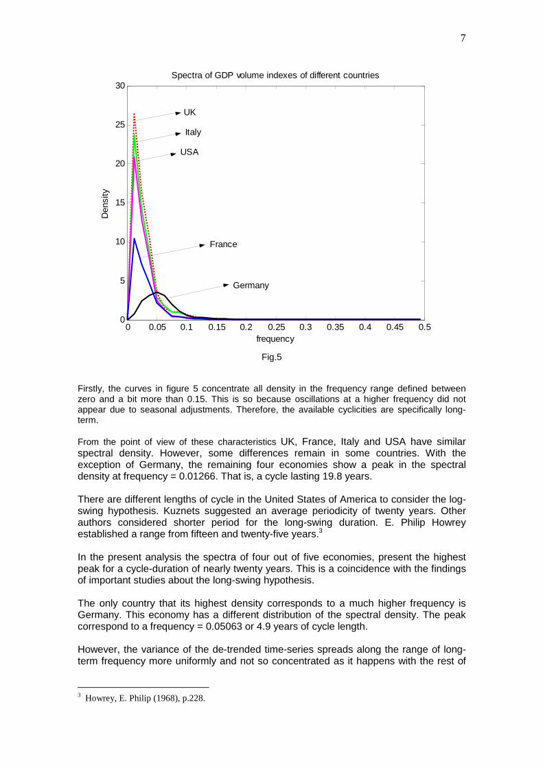
Firstly, the curves in figure 5 concentrate all density in the frequency range defined between zero and a bit more than 0.15. This is so because oscillations at a higher frequency did not appear due to seasonal adjustments. Therefore, the available cyclicities are specifically long-term. From the point of view of these characteristics UK, France, Italy and USA have similar spectral density. However, some differences remain in some countries. With the exception of Germany, the remaining four economies show a peak in the spectral density at frequency = 0.01266. That is, a cycle lasting 19.8 years. There are different lengths of cycle in the United States of America to consider the log-swing hypothesis. Kuznets suggested an average periodicity of twenty years. Other authors considered shorter period for the long-swing duration. E. Philip Howrey established a range from fifteen and twenty-five years.3 In the present analysis the spectra of four out of five economies, present the highest peak for a cycle-duration of nearly twenty years. This is a coincidence with the findings of important studies about the long-swing hypothesis. The only country that its highest density corresponds to a much higher frequency is Germany. This economy has a different distribution of the spectral density. The peak correspond to a frequency = 0.05063 or 4.9 years of cycle length. However, the variance of the de-trended time-series spreads along the range of long-term frequency more uniformly and not so concentrated as it happens with the rest of

3 Howrey, E. Philip (1968), p.228.

8

the economies with a longer length of cycle. Later on, this characteristic will be associated to structural aspects of the German economy. By now, let us concentrate for a while in the remaining four countries that have a relevant peak at a frequency = 0.01266. They share the characteristic that the most relevant cycle corresponds to the hypothesis of long swing of 20 years. There, the highest ordinate of the spectrum corresponds to the United Kingdom, followed successively by Italy, USA and France. Here there are two dimensions to take into account: one is the area below the density function and the other is the measure of the most relevant ordinate. In the case of GDP, the ordering of these two dimensions is coincident. This follows clearly from the table 1, the figure 5 and table 3 later. In general, the value of the integral of the spectrum equals the variance of the de-trended time-series, and the magnitude of the ordinate at a certain frequency depends on the distribution of the variance among frequencies.

0 0.05 0.1 0.15 0.2 0.25 0.3 0.35 0.4 0.45 0.50

50

100

150

200

250

300Spectra of Gross Capital Formation volume indexes

frequency

Den

sity

USA

Italy

UK

France

Germany

Fig, 6

Furthermore, the values of the spectra of the figures 5 and 6, for the relevant range of frequencies, appear in Tables 1 and 2. The highlighted numbers correspond to the peaks in the spectral density function of each economy. In the case of the gross capital formation (GKF), the ordering of countries observed for the GDP variable does not hold. For instance, the area below the curve of UK is bigger than the one for Italy, but the maximum peak-ordinate is higher for Italy with respect to UK. However, Germany and France maintain the smallest variances as can be noted in table 3 as it happened with the GDP variable, but now the US economy attains the

9

maximum within the group. This implies that the range of variation of fixed investment in the US economy is by far larger than any other country in the sample.

Table 1 Spectral density of GDP seasonally adjusted volume indexes

frequency Germany France UK Italy USA

0.00000 2.01E-17 6.53E-15 7.25E-16 1.16E-14 2.90E-15 0.01266 0.7075 10.4327 26.4355 23.6639 20.8239 0.02532 2.3825 7.1032 16.2014 14.0621 12.7251 0.03798 3.1307 4.6517 10.5397 8.7639 7.8537 0.05063 3.5661 2.1471 3.4578 2.8503 2.5362 0.06329 3.1239 1.2851 1.5293 1.7657 1.2533 0.07595 1.9349 0.4576 0.9871 1.0463 0.4201 0.08861 1.1253 0.4203 0.9705 0.9181 0.3985 0.10127 0.5751 0.2604 0.6896 0.5905 0.3001

Table 2

Spectral density of Gross Capital Formation seasonally adjusted volume indexes

frequency Germany France UK Italy USA

0 2.47E-14 9.87E-16 4.84E-13 1.07E-14 2.06E-14 0.012658 11.93865 39.3466 138.79325 156.947 265.4975 0.025316 24.0752 37.5352863 91.271625 89.334125 156.727563 0.037975 27.423225 29.0397975 63.5721 52.754975 94.7017875 0.050633 26.180125 19.8774975 26.3940625 12.3586875 26.2430125 0.063291 17.13105 11.3398975 14.2463375 5.7516625 11.5053813 0.075949 10.1405313 3.71441125 8.2762375 3.1124375 2.885675 0.088608 6.320675 3.45598 6.37118 3.472525 2.0717875

0.10127 2.7118625 2.2951625 4.9320975 3.08767713 1.2041375 France has a smaller variance than UK, Italy and USA but it has a definite peak at frequency = 0.012658 (cycle of about 20 years of length). The table 3 shows the size of variance for de-trended GDP and Gross Capital Formation time-series.

Table 3: Variance of de-trended series

Time-series Country Variance

GDP Germany 3.1484 GDP France 5.0891 GDP UK 11.5083 GDP Italy 10.1838 GDP USA 8.7371

GKF Germany 24.5240 GKF France 28.3139 GKF UK 67.5882 GKF Italy 63.3256 GKF USA 105.0440

10

The variance of residuals obtained when the linear trend is calculated in both variables, is much smaller in Germany and in France than in the USA, Italy and United Kingdom. This accounts for the total variance of the de-trended variable and correspond to smoother cycles with less amplitude. This clearly contrasts with the rest of the economies, and in particular with the USA. This situation repeats itself in the case of the time series of gross capital formation. With the first four countries the peak in density takes place with a similar length as in GDP. On the other hand, in Germany, the most important cycle in capital formation has a length of 6.6 years. It exceeds the duration of its cycle in GDP. From the point of view of long-term cyclical movements, Germany oscillates in economic activity and gross fixed investment much quicker than the rest of economies considered in the sample, but its cycle is more probabilistic. In economics, the cycles identified by the spectrum rarely may represent a deterministic cycle. They are mainly stochastic, or at least, are stylised forms of quasi stochastic periodicities. The case of Germany, both in GDP and GKF the absence of a “thin” spike suggests that they are particularly stochastic. (ii) Relationship of GDP and Gross Capital Formation time-series between each European country and the US economy In this section, the relationship between each European country and the US economy is considered and compared. This part of the analysis and also the next one, will use the bivariate spectral analysis that it is based on the cross spectrum to examine the relationship between two time-series. Remember that in the Spectrum of a given time-series each ordinate is independent from any other ordinate. Therefore, the relationship between two time-series must be considered for a definite frequency. The cross spectrum is usually a complex function and can be written

)(.)()( fquadifcofSYX += (5) The bivariate analysis will be carried in terms of co(f) and quad(f), that is the cospectrum and the quadrature spectrum, which are real functions. The following spectra were derived from the cross spectrum of a pair of variables. They generate other spectra that can be easily interpreted in terms of regression analysis. For example, coherence is a concept very close to R2 in a regression between two variables. Phase is a function of the frequency and represents the average phase shift, here denoted by the average of (φy - φx). If the phase value is zero, both time-series have a synchronous cycle at the given frequency. This means that each starts and ends at the same time. According to the computation of the cross spectrum, the interpretation is the following: If the expression between parentheses is negative, x leads y in t’ periods, and if the expression is bigger than zero, x lags y in t’. The phase spectrum allows identifying leads or lags and measures them in number of periods. The lead/lag length is

11

computed as - φ(f)/2πf. 4 Of course, x corresponds to the US variable and y to the same variable of the European country. The gain function reflects something like a regression coefficient of the relationship between x and y. Finally, the amplitude function reflects the covariation between both variables. Coherence function

xxyyxxyy

yx

yx SS

fquadfco

SS

S

.

)()(

.

222

2 +==κ (6)

Phase function

(7)

If the phase is linear, its slope measures the lag of one series respect of the other. When this linearity does not hold the lag or lead corresponds to a particular frequency. The estimate of lag may be non integer.5 Gain function

)(

)(

fS

fSR

xx

yx

yx = (8)

Cross Amplitude function

))()(()( 22 fquadfocfAyx += (9)

The bivariate study (ii) considers long-term relationship between each European country with the US economy. In other words, the study attempts to detect the relationship of gdp and gross fixed investment of each of the four European countries with respect the American economy. In the table 2 the values of the computed spectra are presented only for a range of low frequency for the sake of simplification, since the most important evidence appears in this range. Table 4. Relationship between each European country and the USA

Gross Domestic Product Gross Capital Formation

Germany-USA

frequency Coherence Phase Gain Amplitude Coherence Phase Gain Amplitude

0 1.0000 0.0000 0.0833 0.0000 1.0000 0.0000 1.0937 0.0000 0.012658 0.6597 0.4212 0.1497 3.1177 0.0798 -1.3916 0.0599 15.9023 0.025316 0.2719 -0.1251 0.2256 2.8710 0.0484 -0.2521 0.0863 13.5208 0.037975 0.2446 -0.2923 0.3122 2.4522 0.1277 -0.5216 0.1923 18.2135

4 Gottman, John M. (1981), p. 303. 5 Newbold, P. (1981), “Some Recent Developments in Time Series Analysis”, International Statistical Review, pp. 54-55.

= −

)(

)(tan)( 1

fco

fquadfφ

12

0.050633 0.5094 -0.4601 0.8463 2.1465 0.5896 -0.4679 0.7669 20.1260 0.063291 0.5695 -0.2947 1.1914 1.4932 0.6641 -0.0639 0.9944 11.4410 0.075949 0.6698 -0.0885 1.7565 0.7379 0.8154 0.4278 1.6927 4.8847 0.088608 0.8008 -0.2652 1.5038 0.5993 0.7426 0.3113 1.5052 3.1185

0.10127 0.8903 -0.4189 1.3060 0.3920 0.7438 -0.2735 1.2942 1.5585

Gross Domestic Product Gross Capital Formation

France-USA

frequency Coherence Phase Gain Amplitude Coherence Phase Gain Amplitude

0 1.0000 0.0000 1.5000 0.0000 1.0000 0.0000 0.2187 0.0000 0.012658 0.9951 -0.0953 0.7061 14.7035 0.9962 -0.3620 0.3842 102.0137 0.025316 0.9545 -0.1552 0.7299 9.2887 0.8323 -0.4272 0.4465 69.9731 0.037975 0.9265 -0.1797 0.7408 5.8179 0.7852 -0.4463 0.4907 46.4682 0.050633 0.8859 -0.3288 0.8660 2.1963 0.8247 -0.5329 0.7903 20.7407 0.063291 0.9023 -0.3144 0.9619 1.2055 0.7917 -0.4804 0.8833 10.1631 0.075949 0.8458 0.0124 0.9598 0.4032 0.7258 0.3140 0.9666 2.7893 0.088608 0.8115 -0.1529 0.9251 0.3687 0.7379 0.3236 1.1095 2.2986

0.10127 0.6981 -0.3073 0.7782 0.2336 0.4362 0.2486 0.9118 1.0979

Gross Domestic Product Gross Capital Formation

UK-USA

frequency Coherence Phase Gain Amplitude Coherence Phase Gain Amplitude

0 1.0000 0.0000 0.5000 0.0000 1.0000 0.0000 4.8437 0.0000 0.012658 0.9705 -0.1635 1.1100 23.1139 0.9828 -0.1856 0.7168 190.2996 0.025316 0.9239 -0.1879 1.0846 13.8015 0.9418 -0.2295 0.7406 116.0703 0.037975 0.8765 -0.1791 1.0845 8.5176 0.8704 -0.2532 0.7644 72.3875 0.050633 0.7248 -0.2531 0.9941 2.5212 0.6780 -0.3589 0.8258 21.6707 0.063291 0.7353 -0.3133 0.9472 1.1872 0.3597 -0.2961 0.6674 7.6789 0.075949 0.8674 0.1659 1.4277 0.5998 0.3137 1.0053 0.9486 2.7372 0.088608 0.9068 0.1109 1.4860 0.5922 0.6162 0.9482 1.3765 2.8519

0.10127 0.8247 0.0994 1.3765 0.4131 0.5567 0.7457 1.5100 1.8183

Gross Domestic Product Gross Capital Formation

Italy-USA

frequency Coherence Phase Gain Amplitude Coherence Phase Gain Amplitude

0 1.0000 0.0000 2.0000 0.0000 1.0001 0.0000 0.7188 0.0000 0.012658 0.9994 -0.0438 1.0657 22.1914 0.9938 -0.1507 0.7665 203.5004 0.025316 0.9236 -0.1270 1.0103 12.8559 0.9165 -0.2124 0.7228 113.2799 0.037975 0.8664 -0.1717 0.9832 7.7221 0.8491 -0.2355 0.6878 65.1323 0.050633 0.6911 -0.4940 0.8813 2.2352 0.5347 -0.5814 0.5018 13.1693 0.063291 0.5900 -0.4481 0.9117 1.1427 0.3713 -0.6652 0.4308 4.9570 0.075949 0.7353 0.0776 1.3533 0.5685 0.6848 0.9317 0.8594 2.4801 0.088608 0.7570 -0.1451 1.3206 0.5263 0.4269 0.8528 0.8459 1.7526

0.10127 0.6396 -0.3504 1.1218 0.3367 0.1152 0.4484 0.5436 0.6546 The coherence spectrum gives an idea of the degree of correlation of both time-series for a given frequency. The significance of the values of the coherence spectrum can be tested as follows from the Bloomfield’s quotation:

13

“Observed values of κ2XY(f) less than σ(0.95)2 should therefore be regarded as not significantly

different from 0,…”6. Then, Table 4 must be tested at a 5% of significance with σσσσ(0.95)2 = 0.568. Any value of coherence in the Table is significantly different from zero if ≥≥≥≥ 0.568. (a) Time-series: GDP The first step in a bivariate analysis is identifying if two series have a cycle at the same frequency. When this happens, it indicates that there is a bivariate relationship. The relationship is also possible if one series has a peak and the other concentrates a smaller quantity of power within the band. In the analysis, the most important spectrum is the coherence. If the correlation exists the other spectra can be successfully interpreted (Gottman). In terms of coherence, Germany has no relationship in the long-swing hypothesis with the USA because there is no coincidence in the peaks of each spectrum. In other words, The cycle corresponding to Germany’s peak spectrum value has no correlation with a similar American cycle. Besides, the lack of correlation persists for slower frequencies except f = 0.012658. Here there is correlation with the long-term cycle in the USA, though this cycle is not relevant for Germany! Then, the correlation arises again for shorter cycles. The latter are not relevant for both countries according to the variance assigned at each frequency. However, the coherence at f = 0.012658 suggests a bivariate relationship, and then it is interesting to see what other spectra derived from the cross spectrum can tell about this relationship. The phase spectrum has a positive sign implying that the US GDP has a lag on the German GDP. The length of the lag measured in quarters is measured as tlag = -φ(f)/2πf = - 0.4212/(2π0.012658) ≅ -5 quarters. This situation implies that the German GDP leads (by 5 quarters) the US GDP in a cycle of 20 years length! Nevertheless, these numbers do not make sense because both spectra do not coincide in identifying a cycle in both countries at the same frequency. For some frequencies higher than f = 0.050633 (where Germany has a peak) coherence becomes stronger and the lag of the US GDP becomes a lead with a length of approximately one quarter. This apparent contradiction can be explained as it follows. The spectrum of USA concentrates an important amount of variance (thin spike) in the f = 0.012658. Immediately, in the neighbourhood of that point the variance declines significantly. For Germany, the picture is quite, different. The peak in the German spectrum takes place at f = 0.050633, but in the neighbourhood of this point the variance is slightly less (wide spike). This implies, that the cycle of the US economy looks like a quasi-deterministic, in Germany, the wide spectrum around f = 0.050633 describes a more pronounced stochastic cycle. Therefore, it is no use to estimate a cycle by regression and should be modelled with autoregressive and moving average terms. Therefore, Germany has no regular cycle. Contrarily, It has a stochastic cycle whose parameters are varying through time. On the other hand, the rest of economies in the sample have regular cycle at f = 0.012658.

6 The estimate of σσσσ(0.95)2 results from 2

2

105.01)95.0( g

g

−−=σ or, as expressed by Bloomfield,

from )1( 2

2

20)95.0( g

g

−−

=σ (Bloomfield, Peter, (2000), p221). Both expressions are equivalent.

14

Therefore, the leads and lags between Germany and USA adopt a random occurrence in the range of frequencies treated. This suggests discarding a regular relationship between both GDP’s for the frequency corresponding to the U.S. peak. This situation poses a clear distinction between the German economy and the American economy. The relevant long-term-swing is different for each of them. The German economy has not a permanent cycle and the amplitude around the trend is smaller. These conditions are so since the German spectra of GDP and GKF suggest the existence of stochastic oscillations with great variation of alternatives. Therefore, it is more reasonable to say that there is no significant stable correlation between the GDP’s of Germany and USA. At the end of the paper, some interpretations of these results will be given in economic terms. In general, a bivariate relationship could be also possible if one series has a peak and the other concentrates a smaller quantity of power within the band but enough to identify a cycle. Therefore, this does not seem to be the case for the relationship between Germany and USA in this study. The information of table 4 shows the spectra of the rest of countries within a band of frequencies that are of interest to the present study. Besides, Table 5 shows the number of quarters of duration of leads and lags. Here a negative figure represents that USA lags while a positive number means a lead. This is the opposite of the sign meaning in the Phase spectrum.

Table 5 Length of Leads & Lags of US GDP on the GDP of other countries (measured in quarters) lead(+)/lag(-) frequency Germany France UK Italy

0 0.012658 -5.3 1.2 2.1 0.6 0.025316 0.8 1.0 1.2 0.8 0.037975 1.2 0.8 0.8 0.7 0.050633 1.4 1.0 0.8 1.6 0.063291 0.7 0.8 0.8 1.1 0.075949 0.2 0.0 -0.3 -0.2 0.088608 0.5 0.3 -0.2 0.3

0.10127 0.7 0.5 -0.2 0.6

The only situation in this graph where US GDP lags a European GDP is when the latter is Germany. In the rest of countries, America leads their economic activities. France, United Kingdom and Italy have high values of coherence with respect of the US GDP. Furthermore, at the frequency 0.012658 take place the maximum spectral value for GDP for the three countries and the USA. In all cases, the coherence value is significantly different from zero. Then the bivariate relationship is accepted in the three countries. Economic activity in the USA has a definite impact in the cycle of the three European countries.

15

The long-term swing is the same for them and coincides with the US long-term swing of twenty years length for the cycle. The longest lead of US GDP lasts 2 quarters and takes place in the relationship with the United Kingdom. The Gain spectrum has positive values in all cases implying that the relationship with the three European countries is positive. The high Gain values take place in UK while the low values correspond in France. Remember that the variance of de-trended time series is small in France and is much closer to the German case. Nevertheless, the spectrum maximum ordinates concentrate a large quantity of variance as if it happens in USA. (b) Time-series: Gross Capital Formation The behaviour of fixed investment presents some interesting differences with the gross domestic product. The relationship between USA and Germany shows a different picture. Remember that the values of coherence are significantly different from zero when reach 0.568 or more, at a level of 5% significance. Coherence in GKF expresses relationship from f = 0.050633 upwards. However, the spectrum peak of GKF of Germany corresponds to f = 0.037975. At this frequency there is no correlation at all. The German GKF spectrum does no present a spike and its shape reminds the case of GDP. It implies the existence of a stochastic cycle. Therefore, there is no reliable systematic correlation between the US oscillation in gross fixed investment and that from Germany. Any result in this sense takes place at random. Generally, there is no systematic relationship between German and American gross fixed investment. Their relevant long-term cycles have different duration. The leads and lags of Table 6 for each country at different frequencies may induce mistake in the case of Germany, The leads of US fixed investment at frequencies 0.012658, 0.025316, and 0.037975 are meaningless since coherence is not significantly different from zero at 5% level.

Table 6 Length of Leads & Lags of US GKF on the GKFof other countries (measured in quarters) lead(+)/lag(-) frequency Germany France UK Italy

0 0.012658 17.5 4.6 2.3 1.9 0.025316 1.6 2.7 1.4 1.3 0.037975 2.2 1.9 1.1 1.0 0.050633 1.5 1.7 1.1 1.8 0.063291 0.2 1.2 0.7 1.7 0.075949 -0.9 -0.7 -2.1 -2.0 0.088608 -0.6 -0.6 -1.7 -1.5

0.10127 0.4 -0.4 -1.2 -0.7

16

Quite a different thing happens with France, United Kingdom and Italy, where the coherence is high and the lead of US fixed investment exceeds the year in France, and attains six months in UK and Italy. These countries share the same cycle with USA and receive an important influence from the American economic activity. The direction of the influence is positive and the amplitude spectrum refers to the level of the cross variation between country investment. In the long run these economies move together in a regular cycle. (iii) Bivariate analysis of dependence of economic activity on fixed investment in the sample. In this part, the analysis intends to detect empirically the dependence of economic activity on gross fixed investment in each country under study. The results for the relevant range of frequencies are shown in Table 7. Let’s start with Germany. The coherence spectrum show significant values at the 5% level except in the case of the cycle of 20 years of duration. Once again, Germany keeps itself away from the experience of the rest of countries. The rest of frequencies in the relevant range used in this table, the coherence is very high, the phase is negative for the lowest frequencies (investment leads GDP), the gain spectrum values are positive and the cross amplitude attains a maximum at frequency 0.05633 (when the GDP spectrum has a peak).

Table 7. Relationship between GDP and GKF per country Germany

frequency Coherence Phase Gain Amplitude

0 1.0000 0.0000 0.0286 0.0000 0.012658 0.4712 -0.6789 0.1671 1.9950 0.025316 0.7346 -0.3015 0.2696 6.4912 0.037975 0.7642 -0.2241 0.2954 8.1000 0.050633 0.8546 -0.1680 0.3412 8.9323 0.063291 0.9045 -0.1286 0.4061 6.9574 0.075949 0.8728 -0.0063 0.4081 4.1384 0.088608 0.8325 0.0728 0.3850 2.4334

0.10127 0.7004 0.2115 0.3854 1.0451 France

frequency Coherence Phase Gain Amplitude

0 1.0000 0.0000 2.5714 0.0000 0.012658 0.9941 0.1989 0.5134 20.2011 0.025316 0.9418 0.1679 0.4222 15.8462 0.037975 0.9289 0.1677 0.3857 11.2020 0.050633 0.9571 0.1475 0.3215 6.3913 0.063291 0.9239 0.1618 0.3236 3.6693 0.075949 0.8452 0.2891 0.3227 1.1985 0.088608 0.8724 0.1854 0.3257 1.1257

0.10127 0.8438 0.0956 0.3094 0.7102

17

UK

frequency Coherence Phase Gain Amplitude

0 1.0000 0.0000 0.0387 0.0000 0.012658 0.9651 -0.0203 0.4287 59.5065 0.025316 0.9323 0.0082 0.4068 37.1307 0.037975 0.8964 0.0576 0.3855 24.5073 0.050633 0.8334 0.0976 0.3304 8.7211 0.063291 0.8537 -0.1149 0.3027 4.3129 0.075949 0.8050 -0.1000 0.3099 2.5645 0.088608 0.8572 -0.1001 0.3614 2.3022

0.10127 0.7921 -0.1080 0.3328 1.6413 Italy

frequency Coherence Phase Gain Amplitude

0 1.0001 0.0000 1.0435 0.0000 0.012658 0.9975 0.0353 0.3878 60.8661 0.025316 0.9913 0.0350 0.3950 35.2891 0.037975 0.9823 0.0274 0.4040 21.3108 0.050633 0.9337 0.0060 0.4640 5.7349 0.063291 0.8597 -0.0091 0.5137 2.9547 0.075949 0.7895 -0.1471 0.5152 1.6035 0.088608 0.7549 -0.1266 0.4468 1.5514

0.10127 0.7688 -0.0363 0.3835 1.1840 USA

frequency Coherence Phase Gain Amplitude

0 1.0000 0.0000 0.3750 0.0000 0.012658 0.9987 -0.0700 0.2799 74.3073 0.025316 0.9951 -0.0705 0.2842 44.5479 0.037975 0.9897 -0.0626 0.2865 27.1305 0.050633 0.9546 -0.0349 0.3037 7.9708 0.063291 0.8753 0.0129 0.3088 3.5528 0.075949 0.7971 0.5215 0.3407 0.9830 0.088608 0.8409 0.5712 0.4022 0.8332

0.10127 0.8224 0.4746 0.4528 0.5452 The rest of countries concentrate their most important spectrum value at frequency 0.012658, that is, at the cycle of twenty years length. The latter is the long-term swing typical of the American economy. .

Table 8 Leads & Lags of GKF on the GDP per country (measured in quarters) lead(+)/lag(-)

frequency Germany France United

Kingdom Italy USA

0 0.012658 8.5 -2.5 0.3 -0.4 0.9 0.025316 1.9 -1.1 -0.1 -0.2 0.4 0.037975 0.9 -0.7 -0.2 -0.1 0.3 0.050633 0.5 -0.5 -0.3 0.0 0.1

18

0.063291 0.3 -0.4 0.3 0.0 0.0 0.075949 0.0 -0.6 0.2 0.3 -1.1 0.088608 -0.1 -0.3 0.2 0.2 -1.0

0.10127 -0.3 -0.2 0.2 0.1 -0.7

Here, it is interesting to clarify possible meanings of the lead and lag of gross fixed investment on gross domestic product. The simplest way to explain these two concepts is that lead of investment on GDP implies a supply decision while a lag of investment with respect to GDP correspond to decision taken from the demand side. However, these definitions are very broad, and in this case, more precision is required, mainly in the sense that the decisions are taken in a long-term context. El demand side looks easier to explain in the shorter runs. In our case, the explanation has to remain in the long-term. Nevertheless, gross fixed investment can be classified into plant expansion and heavy equipment promoted by plans for the future, and investment in fixed capital for maintenance of the stock and intensification of the rhythm of production. A long-term-cycle may include both kinds of fixed investment though in the long-term the first kind is much important than the second. The length of leads and lags in fixed investment on gross domestic product are very short as can be seen in Table 8. The USA and Germany totally, and the UK partially only in the long term swing of 20 years, are the only economies where the supply side definitely governs the long-run oscillations. France shows a lag of investment with respect of GDP. In the case Italy the lag are very small so it could be considered approximately synchronous. General Comparisons One way to compare visually the 20-year-cycle for the four countries except Germany is to look at the figure 7. Here, one can see differences in amplitude and phase shift. The model of each country cycle was obtained by a harmonic regression. A quick and simple way to compare numerically the long-swing cycle could be through the harmonic regression parameters used to estimate the cycle of each country. They can be complemented with the visual representation of each fitted cycle. The cycle model considered was: xt = A cos(2πf t + φ) + εt (10) where, the coefficient A represents the amplitude, 2πf is the angular frequency, t is the time measured in quarters, and φ is the phase-shift measured in radians. The larger the value of A, the greater is the displacement around the trend. The angular frequency represents the number of complete cycles in 2π units of time. Equation (10) is built from the harmonic regression equation xt = A1 cos(2πf t) + A2 sin(2πf t) (11) That is, the parameters of (10) emerge from A1 and A2.

19

The transformation of (11) into (10) is done by considering that the latter expresses the cosine of a sum of angles. So that equation (10) can be written xt = A cos(φ)cos(2πf t)+[-Asin(φ)]sin(2πft) (12) Therefore, A1 = A cos(φ) and A2 = - A sin(φ) (13) From here, it follows that A1

2 + A22 = A2 with the help of cos2(α) + sin2(α) = 1.

From (13) the parameter φ should be obtained as a function of the parameters A1 and A2 of the harmonic regression. However, Bloomfield pointed out that there are some possible combinations of signs and zero values between the parameters of the harmonic regression that render incomplete the equation (13) to solve the values of φ.7 Below, the table describes the Bloomfield’s set of alternative solutions for the phase-shift depending on the sign and values of the coefficients obtained in the harmonic regression. Although the second and third cases have been corrected in sign since the Bloomfield conditions seem to be misprinted in his book.

Table 9 arctan (-A2/A1) A1>0 arctan (-A2/A1) + π π π π A1<0, A2>0

φ =φ =φ =φ = arctan (-A2/A1) - π π π π A1<0,A2≤≤≤≤0 -(ππππ/2), A1=0, A2>0 ππππ/2 A1=0, A2<0 arbitrary A1=0, A2=0

The correction made here consisted in changing the sign of π in the second and third line of the table. There is proximity of the British and Italian cycles of 20-year-length with the equivalent US cycle (figure 7). The estimate of the long-term cycle of nearly 20-year-length for France, United Kingdom, Italy and USA for gross domestic product and gross capital formation can be used to determine in what part of the periodic trajectory each economy is placed. At the end of both time series, GDP and GKF, for each country the cycle is arriving at its lowest level. The depression is reaching at the end and a new period of expansion is ready to start. If these economies are moving along this long-term oscillation, then it is likely to expect to reach the trend level in approximately five years time. The estimated cycles are a stylised version of the real movement, and the actual levels of GDP and GKF are a sum of other components, particularly stochastic. Therefore, the path will take place with ups and downs. However, the long-term movement will be upwards.

7 Bloomfield, P, (2000), p.13. Bloomfield provides a full solution, which gives an answer in the interval (-1/2, ½]. He covers three alternative cases. Two of them has probably been misprinted in the book and are wrong. One of those coincides with the case of the present study, which is when A1 and A2 are negative; therefore, they were corrected and included in the next table.

20

0 10 20 30 40 50 60 70 80-4

-3

-2

-1

0

1

2

3

4GDP cycle of 20 years duration

quarters

GD

P

France

Italy

UK

USA

Fig. 7

The main difference of the French cycle with respect to the two European countries and the USA is significantly smaller amplitude. The comparisons of these spectra can be more precisely done through the parameters of equation (10). Table 10 provides

Table 10. Gross Domestic

Product. Parameters of the Cyclical Model Country A1 A2 A φ R squared (t statistic) (t statistic)

France -2.4679 -0.6036 2.54 -3.38 Rsq.=0.651 (-11.63) (-2.84)

UK -3.6316 -1.2589 3.84 -3.48 Rsq.=0.659 (-11.51) (-3.99)

Italy -3.6962 -0.6814 3.76 -3.32 Rsq.=0.712 (-13.55) (-2.50)

USA -3.5137 -0.4860 3.55 -3.28 Rsq.=0.739 (-14.62) (-2.02)

the data about the harmonic regression and the parameters of the sinusoidal model. In the first column appear the country and the R2 of the linear harmonic regression. The following two columns show the coefficients and their t statistics of the harmonic regression. Then, the last two columns contain the amplitude and phase-shift coefficients in the model (equation 10). The coefficient A varies directly with the magnitude of the amplitude of the change in the cycle. On the other hand, the greater the value of the phase-shift parameter, the bigger is the displacement of the periodic function to the left. With respect to the GDP variable (Table 10), the ranking of the countries according to the decreasing phase-shift shows that the highest amplitude corresponds to

21

United Kingdom, followed by Italy and USA, in that order. The ranking of the countries according to the decreasing length of phase-shift is USA, Italy, France and United Kingdom. In figure 7, this ranking is clear where the cyclical variable intercepts the value 0 of the ordinate. An analogous examination about gross capital formation arises from Table 11 and figure 8. Gross fixed investment is a more sensitive variable than output. Now, the highest amplitude corresponds to USA. The following countries are located in a declining scale with respect to amplitude of cyclical movement. Quite differently as in the case of GDP, Italy exhibits greater amplitude than Great Britain.

Table 11. Gross Capital Formation.

Parameters of the Cyclical Model

Country A1 A2 A φ R squared (t statistic) (t statistic)

France -4.4061 -2.0473 4.86 -3.58 Rsq.=0.428 (-6.88) (-3.2) UK -8.5444 -2.1422 8.81 -3.39 Rsq.=0.589 (-10.19) (-2.55) Italy -9.4966 -2.1968 9.75 -3.37 Rsq.=0.770 (-15.63) (-3.62)

USA -12.6497 -0.7487 12.67 -3.20 Rsq.=0.784 (-16.70) (-0.99)

The phase-shift ordering is not very different from what happened to the GDP variable, except that UK exchanged places with France. Now UK has the smallest φ of the group. The harmonic regression about gross capital formation of USA has the coefficient A2 not significantly different from zero, but this characteristic does not modify the rank of Table 11. The USA is a leading country in this group of advanced countries, both in economic activity and fixed capital formation, This country shows broader fluctuations than those that follow their pace with respect to gross capital formation.. These models emphasise the basic characteristics of each long term cycle. The bigger impact of oscillations on investment takes place in the leading country, both upwards and downwards. With respect to economic activity, the situation is different. In figure 7, the cyclical path of the leading economy moves within the range determined by the evolution of the countries receiving the influence. Here, the amplitude differences are not substantial. Now is the moment to consider the behaviour of Germany which was postponed due to the inability to identify a stable cycle of length comparable to the U.S. long swing hypothesis.

22

0 10 20 30 40 50 60 70 80-15

-10

-5

0

5

10

15GKF cycle of 20 years duration

quarters

GK

F

USA

Italy

UK

France

Fig. 8

So far, the twenty years cycles obtained by regression provide basic information to make comparisons among three European countries and the USA. As mentioned above, the German case had to be described by a dynamic model because no regular cycle seems to be identifiable. The models computed for GDP and GKF are the following: Germany GDP and GKF behaviour as modelled. yt = 0.8179 yt-1 + 0.3371 et-1 + et

(9.26) (2.14) No. obs. = 79 Wald chi2 = 190.51 Prob > Chi2 = 0.0000 where, yt = de-trended German GDP. Portmanteau test for white noise --------------------------------------- Portmanteau (Q) statistic = 32.7282 Prob > chi2(37) = 0.6696

xt = 0.8537xt-1 + 0.0585 ηt-1 + ηt (9.65) (0.43) No. obs. = 79 Wald chi2 = 150.08 Prob > Chi2 = 0.0000

23

where, xt = de-trended German GKF Portmanteau test for white noise --------------------------------------- Portmanteau (Q) statistic = 33.8871 Prob > chi2(37) = 0.6158

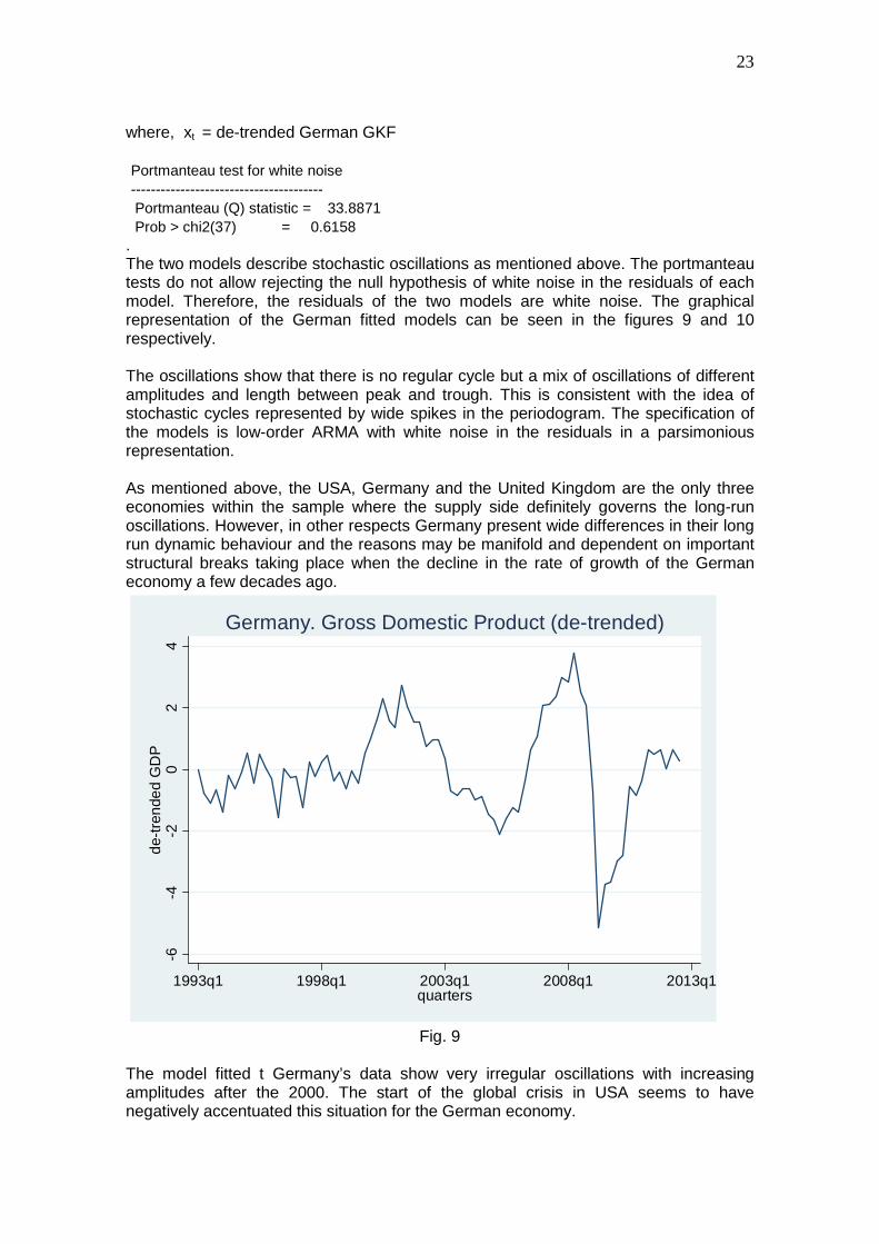
. The two models describe stochastic oscillations as mentioned above. The portmanteau tests do not allow rejecting the null hypothesis of white noise in the residuals of each model. Therefore, the residuals of the two models are white noise. The graphical representation of the German fitted models can be seen in the figures 9 and 10 respectively. The oscillations show that there is no regular cycle but a mix of oscillations of different amplitudes and length between peak and trough. This is consistent with the idea of stochastic cycles represented by wide spikes in the periodogram. The specification of the models is low-order ARMA with white noise in the residuals in a parsimonious representation. As mentioned above, the USA, Germany and the United Kingdom are the only three economies within the sample where the supply side definitely governs the long-run oscillations. However, in other respects Germany present wide differences in their long run dynamic behaviour and the reasons may be manifold and dependent on important structural breaks taking place when the decline in the rate of growth of the German economy a few decades ago.

-6-4

-20

24

de-t

rend

ed G

DP

1993q1 1998q1 2003q1 2008q1 2013q1quarters

Germany. Gross Domestic Product (de-trended)

Fig. 9

The model fitted t Germany’s data show very irregular oscillations with increasing amplitudes after the 2000. The start of the global crisis in USA seems to have negatively accentuated this situation for the German economy.

24

-10

-50

510

de-t

rend

ed G

KF

1993q1 1998q1 2003q1 2008q1 2013q1quarters

Germany. Gross Capital Formation (de-trended)

Fig.10

The model about gross capital formation follows similar lines to the one about GDP (figure 10) but once the global crisis began the amplitudes seem to narrow. However, this gross fixed investment is aimed to domestic production, while Germany is an important exporter that produces in countries where wages are low. In the next section, Germany’s long-term economic behaviour will be explained in more detail. Then it will be possible to understand its differences with respect to other economies in the sample. Concluding Remarks In this study, the aim was placed in five countries of the Group of Seven, in particular, European and US economies. Both Japan and Canada were not taken in consideration. The reason of such a choice was detecting some possible relationships between the US economy and the most advanced economies of Europe. The relationships examined here were those concerning with the long run, in particular the long swing hypothesis once exposed by Kuznets, that is, the economic cycle of nearly twenty-years-length which was identified with the spectral analysis with the exception of the German economy. Here. It is expected that the way out of the present world crisis will be along some part of the path of a long term cycle common to the most important economies. This belief is based on the idea that it is more likely to recover in that way rather than the hope that the world economy moves in an extremely long cycle that could also involve the 1930’s depression. Now, after knowing the results, one would like to have included more countries in the analysis but the scope would have been widened too much outside the content of the present paper.

25

The bivariate spectral analysis showed that there is a lead of the US economy over United Kingdom, France and Italy in terms of gross domestic product and gross capital formation. These economies have some differences among themselves but they share the same twenty-year-cycle. A quite different case is Germany. Its data does not provide evidence of sharing a long-term cycle like the rest of countries in the sample. Moreover, Germany does not have a regular cycle of twenty-year-length. Its spectrum shows a stochastic cycle with wide spike in the periodogram. This means that the oscillations in economic activity and gross fixed investment move randomly with changing amplitudes, lengths and so on. Here, it cannot be detected a definite lead or lag on part of the American economy. Germany is the fifth economy in the world after USA, China, Japan, and India. Therefore, it is interesting to consider where might be the explanation for such results of the spectral analysis. West Germany underwent a sustained process of economic growth during the first decades of its existence after the Second World War. The annual growth rates averaged 8.2% in 1950-1960; 4.4% in 1960-1970; 2.8% in 1970-1980; 2.2% in 1980-1990. After 1990 the rate of growth of Germany entered into a period of declination with high degrees of unemployment. Between 2000 and 2010, the unemployment rate moved around 9.6 and 11.0 %. The analysis of Ahearn and Belkin of the Congressional Research Service attributes the declining of the German rate of growth to the following factors: (i) The high costs of integrating East Germany to the country; (ii) The Social welfare system creates transfers undermining the incentives to employ and invest; and (iii) The economy became extremely dependent on exports. The main exports were cars, precision machinery and chemicals. The Congressional Report says that Germany maintained its competitiveness by outsourcing and off shoring their labour intensive parts of production to countries with low wages in Eastern Europe. Besides, Germany followed a policy of keeping wages low for very long periods. Therefore, the expansion of exports did not solve problems of production and unemployment in the country. The three factors producing a declining rhythm of growth cannot be considered as probable causes of the particular stochastic cycle in the long term. Factors (i) and (ii) produce transfers of resources in the form of subsidies granted by the State. The other European countries in the sample have also similar transfers, for other reasons perhaps, and they still have a regular cycle. Nevertheless, the factor (iii) may be a main determinant of the stochastic cycle detected in Germany.8 The dynamic behaviour in production and investment of exports in that country mainly responds to conditions determined abroad and distributed in a broad horizon. On the other hand, the decisions based in conditions determined inside

8 “Various data illustrate the growing role that exports have played in Germany’s economy. In 1950, exports, represented the 9.3% of GDP. Once the post-war economic boom got under way, exports rose to 17.2% of GDP in 1960. The rise continued to 23.8% in 1970, to 26.7% in 1980, and to 33% in 1990. By 2008, German exports were accounting for 47% of GDP, compared to less than 20% in Japan and about 13% in the United States”, Ahearn, Raymond J. and Belkin Paul, (2010), p. 10.

26

the economy presumably play a minor role. The Congressional Research Report asserts, “the increase in exports cannot automatically be equated anymore with a commensurate increase in domestic production and employment” The main difference between the three European countries, the US economy and Germany seems to be the degree of export orientation of production of the latter. The degree of state interference in the economy may exist almost in most of the countries with different intensities. The data of table 12 is sufficient to compare the relative importance of exports with respect to the gross domestic product of the five countries of the sample. Let us take the average X/GDP for the total of advanced economies (35 countries) considered in the IMF Report. X denotes exports. For instance, the US ratio is (X/GDP) (16/37.7) = 0.42. The US ratio of exports to GDP is a 42% of the average ratio of 35 advanced economies. The German ratio is (X/GDP) (12.9/7.7) = 1.68. That is a 68 % bigger than the average ratio of advanced economies. The French ratio is only a 6% higher than the average taken as reference while, the Italian and British ratios coincide with the reference level.

Table 12 Advanced economies in 2012 according to the IMF . Shares %

GDP Exports Population

Adv.econ. World Adv.econ. World Adv.econ.

World

Advanced economies (35 countries) 100.0 50.1 100.0 61.2 100.0 14.9 USA 37.7 18.9 16 9.8 30.5 4.5 Germany 7.7 3.8 12.9 7.9 7.9 1.2 France 5.4 2.7 5.7 3.5 6.2 0.9 Italy 4.4 2.2 4.4 2.7 5.9 0.9 United Kingdom 5.6 2.8 5.6 3.4 6.1 0.9 The GDP shares are based on the purchasing-power parity valuation of economies’ GDP. Source: IMF. World Economic Outlook - April 2013

. The German ratio is higher than the mean, the USA’s is lower than the mean, and in France, Italy and the United Kingdom the ratios are equal to the mean of the 35 advanced economies of the World. The dependence on the foreign demand for exports in conditions of global depression means vulnerabilities in the German economy in case o global crisis. The rest of the countries within the sample, shares the long-term cycle of 20 years length. They are in a different situation respect of Germany. Their economies rely much more on domestic consumption and investment while the latter depends mainly on exports.

27

The spectral analysis show that the long-term cycle variance of Germany and France are below the variance of the USA in terms of GDP behaviour. On the other side, the United Kingdom and Italy have larger variance than the USA. The larger variances are associated with sharp fluctuations. It may be probable that higher degree of state intervention in long run decisions may reduce the amplitude of the fluctuations while less intervention gives more room to market interplay. The spectral analysis about gross capital formation reasserts more clearly, that mentioned in the previous paragraph. The long term-cycle variances are larger in the case of USA, UK and Italy. The lowest variances correspond to France and Germany. The times of the leads of the US GDP on the European countries are 2.1 quarters for UK; 1.2 quarters for France; and 0.6 quarters for Italy. In the case of gross capital formation, the US GKF leads are 4.6 time units for France; 2.3 time units for UK; and 1.9 quarters for Italy. The United Kingdom and Italy react sooner than France does. It is likely that the lead of the USA has relation with their foreign investment in the European country and the conditions of the labour market in countries, regulatory schemes and other factors affecting profitability. The longer is the delay in response of the European country in the case of GDP, implies that US foreign investment finds less favourable operating conditions in the market abroad. The opposite happens when the delay is shorter. In the case of gross capital formation, the same applies with respect to new additions of fixed capital abroad, In these matters, the long-term economic policies prevailing in the European country may be responsible of the context within which the time delays in the relationship take place. In the course of this paper, it is present the assumption that the way out of the present global economic crisis is taking place in a long-term cycle, at least, in part of it. The spectral analysis allows expecting that the most advanced economies in the world would move together, each with their own characteristics. The process of recovery will take some time from now in modifying the economic structure of several economies, but this path pre-announces the end of the crisis. The regular long-term cycles fitted for UK, France, Italy and USA indicate that the lowest point is very near and a new period of recovery starts at least for the most advanced economies. Nevertheless, this process will have will be successful in restoring confidence and incentivising investment in different parts of the world. Perhaps, it takes nearly five years to reach trend levels. The German economy will also reactivate with the other European countries; however, this behaviour can be forecasted, from what the entrepreneurs do abroad rather than from what is really happening on inside the economy. Their optimum allocation of resources seems to play a better role abroad than inside its own economy.

28

References * Ahearn, Raymond J. and Belkin Paul, (2010), “The German Economy and U.S.-German Economic Relations”, Congressional Research Service Report, (January 27, 2010). Library of Congress, Washington D.C., USA. * Bloomfield, Peter, (2000), “Fourier analysis of time series: an introduction”, Wiley Series in Probability and Statistics, John Wiley & Sons, second Edition, U.S.A. * Gottman, John M. (1981), “Time-series Analysis. A comprehensive introduction for social scientists”, Cambridge University Press. * Granger, W.J. and Newbold, Paul, (1986) “Forecasting Economic Time Series”, Second Edition, Academic Press, Inc. * Howrey, E. Philip, (1968), “A Spectrum Analysis of the Long-Swing Hypothesis”, International Economic Review, Vol. 9, Nº 2, pp.228-252. * Newbold, P. (1981), “Some Recent Developments in Time series Analysis”, International Statistical Review, Vol. 49, No. 1, pp. 53-66. * O.E.C.D Statistics, B1_GE: Gross Domestic Product – expenditure approach. VIXOBSA, OECD reference year, seasonally adjusted. Quarterly. Period: 1993q1-2012q3. data extracted on 03 Jun 2013 22:16 UTC (GMT) from OECD.Stat * O.E.C.D Statistics, P51: Gross Fixed Capital Formation, VIXOBSA, OECD reference year, seasonally adjusted. Quarterly. Period: 1993q1-2012q3. data extracted on 04 Jun 2013 13:34 UTC (GMT) from OECD.Stat