
An Underwater Acoustic Telemetry Modem for Eco · PDF fileAn Underwater Acoustic Telemetry...
30
1 An Underwater Acoustic Telemetry Modem for Eco-Sensing * Ronald A. Iltis, Ryan Kastner, and Hua Lee Daniel Doonan, Tricia Fu, Rachael Moore and Maurice Chin Department of Electrical and Computer Engineering University of California, Santa Barbara, CA 93106-9560 {iltis,kastner,lee}@ece.ucsb.edu * This work was supported in part by the W.M. Keck Foundation and UCSB Marine Sciences Institute.
Transcript of An Underwater Acoustic Telemetry Modem for Eco · PDF fileAn Underwater Acoustic Telemetry...
1
An Underwater Acoustic Telemetry Modem for Eco-Sensing*
Ronald A. Iltis, Ryan Kastner, and Hua Lee Daniel Doonan, Tricia Fu, Rachael Moore and Maurice Chin
Department of Electrical and Computer EngineeringUniversity of California,
Santa Barbara, CA 93106-9560{iltis,kastner,lee}@ece.ucsb.edu
*This work was supported in part by the W.M. Keck Foundation and UCSB Marine Sciences Institute.
2
Dock
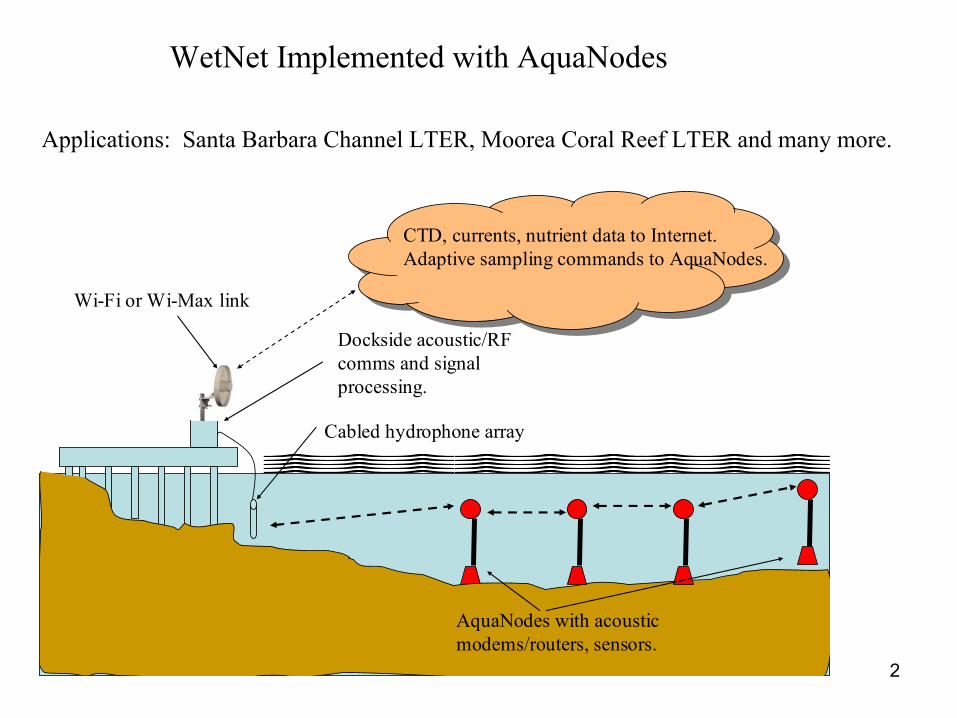
AquaNodes with acoustic modems/routers, sensors.
Dockside acoustic/RF comms and signal processing.
Cabled hydrophone array
Wi-Fi or Wi-Max link
CTD, currents, nutrient data to Internet. Adaptive sampling commands to AquaNodes.
WetNet Implemented with AquaNodes
Applications: Santa Barbara Channel LTER, Moorea Coral Reef LTER and many more.
3
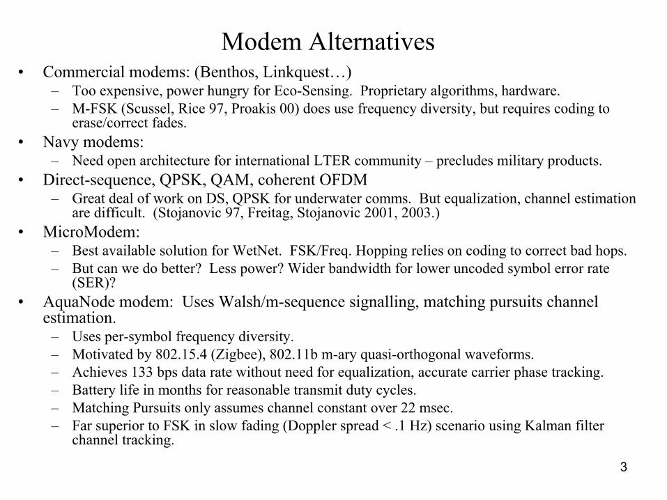
Modem Alternatives• Commercial modems: (Benthos, Linkquest…)
– Too expensive, power hungry for Eco-Sensing. Proprietary algorithms, hardware.– M-FSK (Scussel, Rice 97, Proakis 00) does use frequency diversity, but requires coding to
erase/correct fades.• Navy modems:
– Need open architecture for international LTER community – precludes military products.• Direct-sequence, QPSK, QAM, coherent OFDM
– Great deal of work on DS, QPSK for underwater comms. But equalization, channel estimation are difficult. (Stojanovic 97, Freitag, Stojanovic 2001, 2003.)
• MicroModem: – Best available solution for WetNet. FSK/Freq. Hopping relies on coding to correct bad hops.– But can we do better? Less power? Wider bandwidth for lower uncoded symbol error rate
(SER)? • AquaNode modem: Uses Walsh/m-sequence signalling, matching pursuits channel
estimation.– Uses per-symbol frequency diversity.– Motivated by 802.15.4 (Zigbee), 802.11b m-ary quasi-orthogonal waveforms.– Achieves 133 bps data rate without need for equalization, accurate carrier phase tracking.– Battery life in months for reasonable transmit duty cycles.– Matching Pursuits only assumes channel constant over 22 msec.– Far superior to FSK in slow fading (Doppler spread < .1 Hz) scenario using Kalman filter
channel tracking.
4
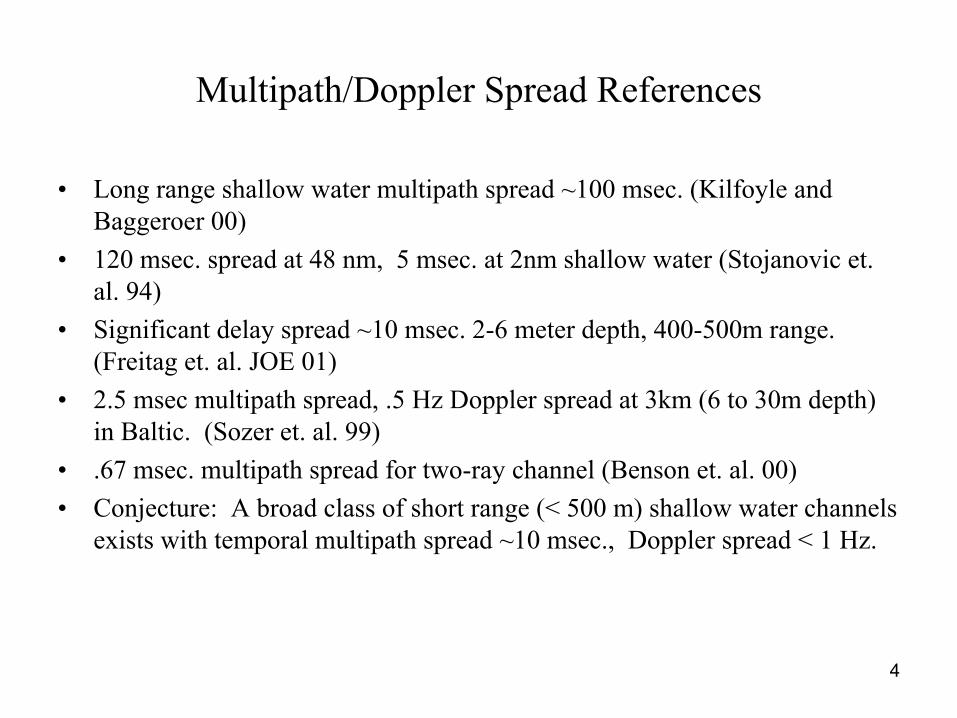
Multipath/Doppler Spread References
• Long range shallow water multipath spread ~100 msec. (Kilfoyle and Baggeroer 00)
• 120 msec. spread at 48 nm, 5 msec. at 2nm shallow water (Stojanovic et. al. 94)
• Significant delay spread ~10 msec. 2-6 meter depth, 400-500m range. (Freitag et. al. JOE 01)
• 2.5 msec multipath spread, .5 Hz Doppler spread at 3km (6 to 30m depth) in Baltic. (Sozer et. al. 99)
• .67 msec. multipath spread for two-ray channel (Benson et. al. 00)• Conjecture: A broad class of short range (< 500 m) shallow water channels
exists with temporal multipath spread ~10 msec., Doppler spread < 1 Hz.
5
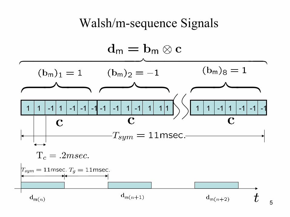
Walsh/m-sequence Signals
1 1 -1 1 -1 -1-1 1 1 -1 1 -1 -1-1-1 -1 1 -1 1 1 1
876 87687644444444 844444444 76
Tc = .2msec.
6
Motivation for Walsh/m-sequence Waveforms
• Wideband (5 kHz) yields frequency diversity.• 3 bits/symbol yields 10log3 = 4.8 dB coding
gain relative to binary FSK.• Does not require accurate phase tracking for
detection (c.f. QPSK, QAM.)• Time-guard band eliminates need for
equalization.• Sparse channel estimation easily implemented
via Matching Pursuits.
7
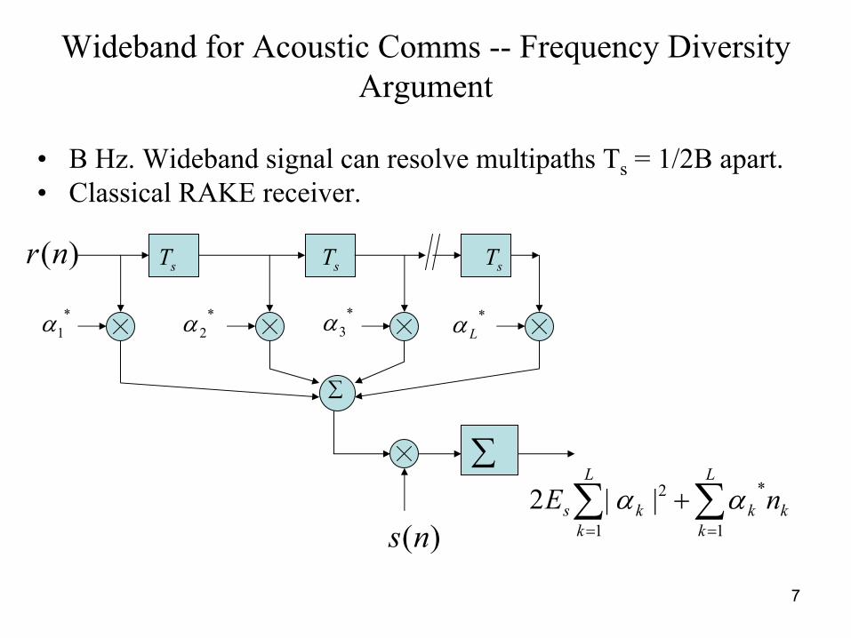
Wideband for Acoustic Comms -- Frequency Diversity Argument
• B Hz. Wideband signal can resolve multipaths Ts = 1/2B apart.• Classical RAKE receiver.
∑
)(nr
k
L
kk
L
kks nE ∑∑
==
+|1
*
1
2|2 αα
*1α
*2α
*3α
*Lα
sT sT sT
∑
)(ns
8
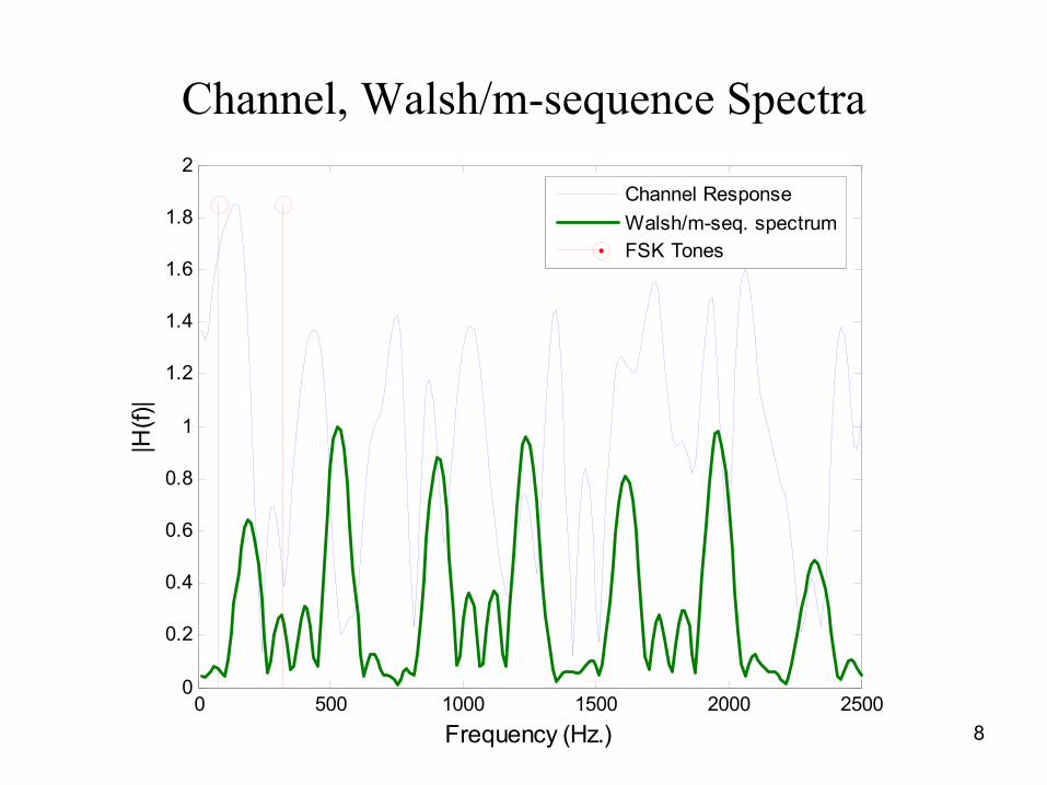
Channel, Walsh/m-sequence Spectra
0 500 1000 1500 2000 25000
0.2
0.4
0.6
0.8
1
1.2
1.4
1.6
1.8
2
Frequency (Hz.)
|H(f)
|
Channel ResponseWalsh/m-seq. spectrumFSK Tones
9
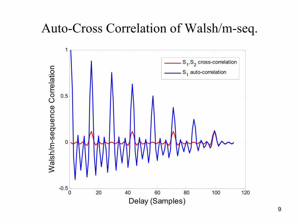
Auto-Cross Correlation of Walsh/m-seq.
0 20 40 60 80 100 120-0.5
0
0.5
1
Delay (Samples)
Wal
sh/m
-seq
uenc
e C
orre
latio
nS1,S2 cross-correlation
S1 auto-correlation
10
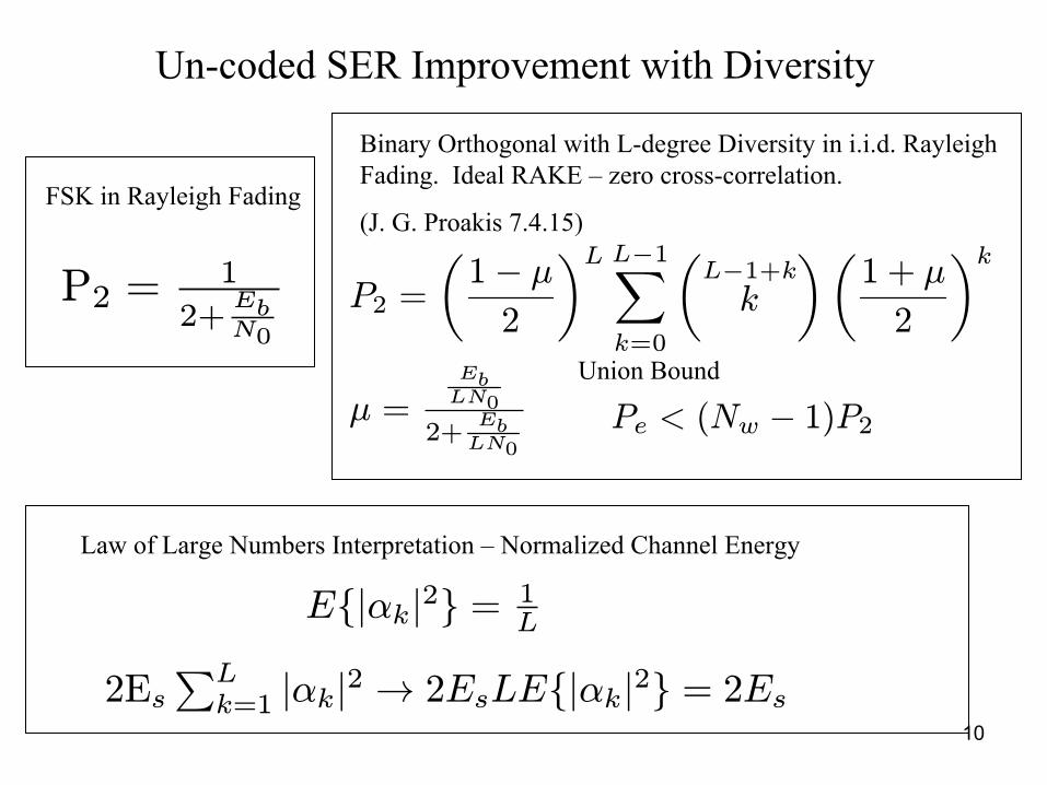
Un-coded SER Improvement with Diversity
FSK in Rayleigh Fading
Binary Orthogonal with L-degree Diversity in i.i.d. RayleighFading. Ideal RAKE – zero cross-correlation.
(J. G. Proakis 7.4.15)
P2 =1
2+EbN0
Union Bound
Pe < (Nw − 1)P2µ =EbLN0
2+EbLN0
Law of Large Numbers Interpretation – Normalized Channel Energy
E{|αk|2} = 1L
2EsPLk=1 |αk|2 → 2EsLE{|αk|2} = 2Es
P2 =
µ1− µ2
¶L L−1Xk=0
µL−1+kk
¶µ1 + µ
2
¶k
11
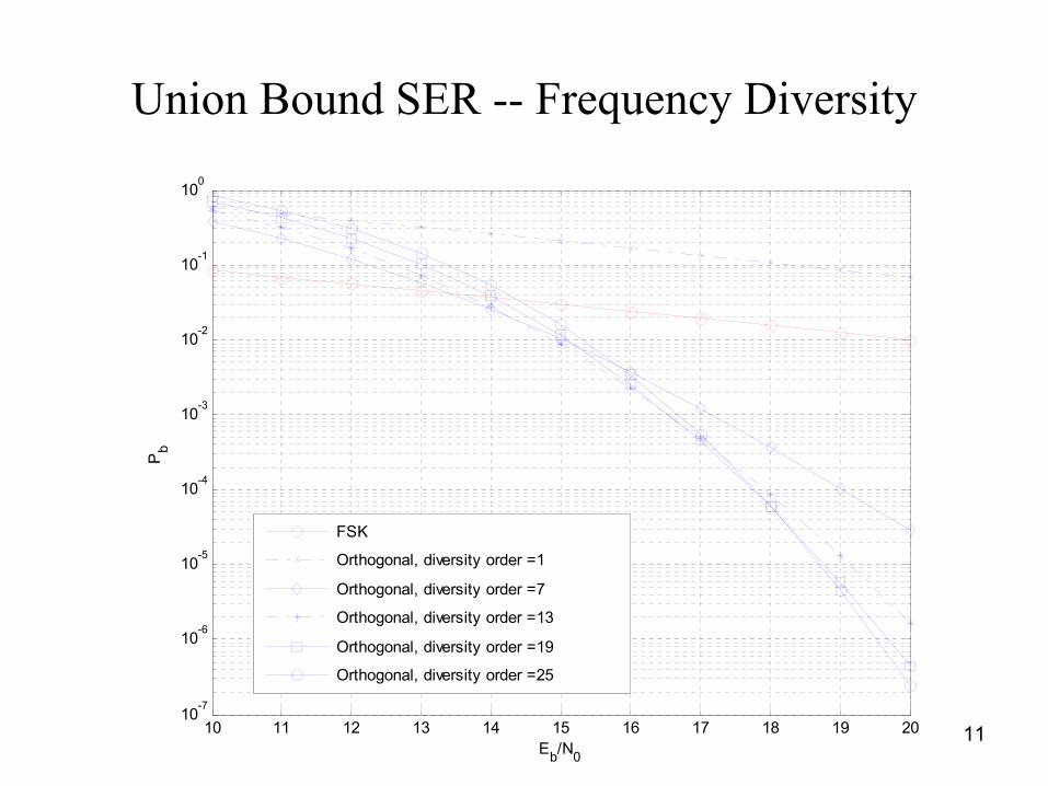
Union Bound SER -- Frequency Diversity
10 11 12 13 14 15 16 17 18 19 2010-7
10-6
10-5
10-4
10-3
10-2
10-1
100
Eb/N0
Pb
FSK
Orthogonal, diversity order =1
Orthogonal, diversity order =7
Orthogonal, diversity order =13
Orthogonal, diversity order =19
Orthogonal, diversity order =25
12
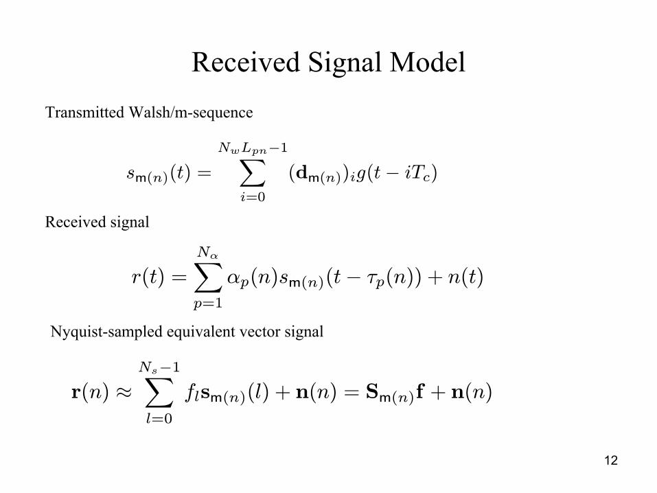
Received Signal Model
r(t) =
NαXp=1
αp(n)sm(n)(t− τp(n)) + n(t)
Transmitted Walsh/m-sequence
Received signal
Nyquist-sampled equivalent vector signal
sm(n)(t) =
NwLpn−1Xi=0
(dm(n))ig(t− iTc)
r(n) ≈Ns−1Xl=0
flsm(n)(l) + n(n) = Sm(n)f + n(n)
13
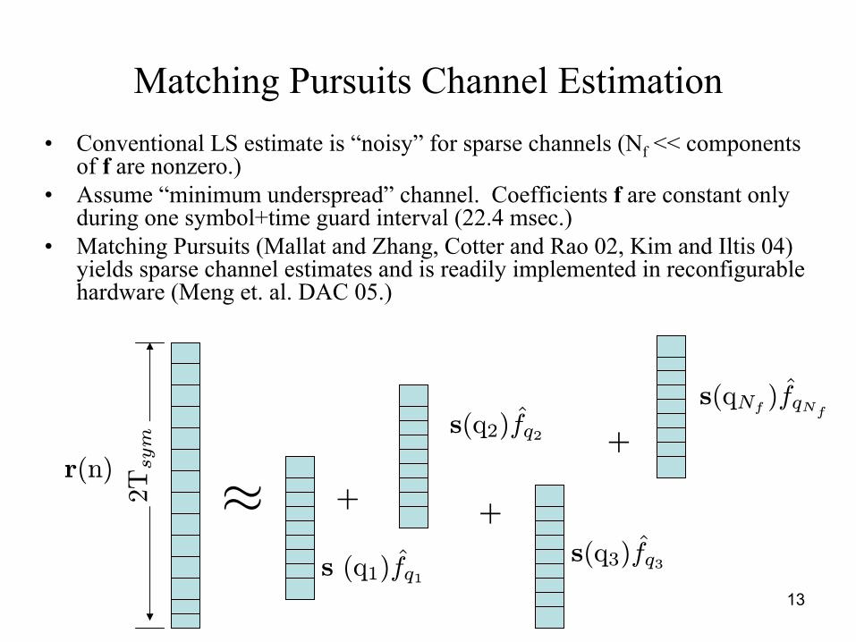
Matching Pursuits Channel Estimation• Conventional LS estimate is “noisy” for sparse channels (Nf << components
of f are nonzero.)• Assume “minimum underspread” channel. Coefficients f are constant only
during one symbol+time guard interval (22.4 msec.)• Matching Pursuits (Mallat and Zhang, Cotter and Rao 02, Kim and Iltis 04)
yields sparse channel estimates and is readily implemented in reconfigurable hardware (Meng et. al. DAC 05.)
r(n) ≈2 Tsym
s (q1)f̂q1
s(q2)f̂q2
s(q3)f̂q3
s(qNf)f̂qNf
++
+
14
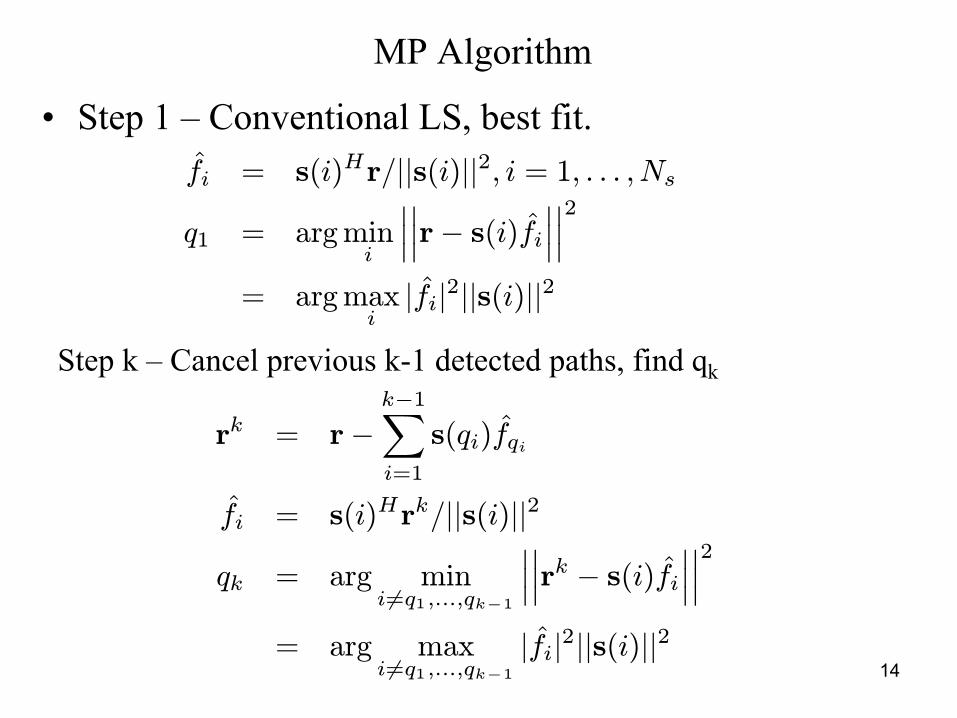
MP Algorithm
• Step 1 – Conventional LS, best fit.
Step k – Cancel previous k-1 detected paths, find qk
f̂i = s(i)Hr/||s(i)||2, i = 1, . . . , Nsq1 = argmin
i
¯̄̄¯̄̄r− s(i)f̂i
¯̄̄¯̄̄2= argmax
i|f̂i|2||s(i)||2
rk = r−k−1Xi=1
s(qi)f̂qi
f̂i = s(i)Hrk/||s(i)||2
qk = arg mini 6=q1,...,qk−1
¯̄̄¯̄̄rk − s(i)f̂i
¯̄̄¯̄̄2= arg max
i 6=q1,...,qk−1|f̂i|2||s(i)||2
15
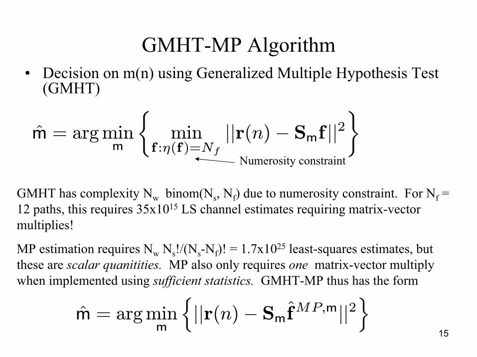
GMHT-MP Algorithm• Decision on m(n) using Generalized Multiple Hypothesis Test
(GMHT)
m̂ = argminm
½min
f :η(f)=Nf
||r(n)− Smf ||2¾
Numerosity constraint
GMHT has complexity Nw binom(Ns, Nf) due to numerosity constraint. For Nf = 12 paths, this requires 35x1015 LS channel estimates requiring matrix-vector multiplies!
MP estimation requires Nw Ns!/(Ns-Nf)! = 1.7x1025 least-squares estimates, but these are scalar quanitities. MP also only requires one matrix-vector multiply when implemented using sufficient statistics. GMHT-MP thus has the form
m̂ = argminm
n||r(n)− Smf̂MP,m||2
o
16
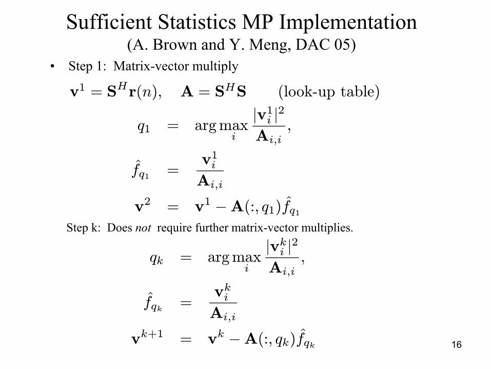
Sufficient Statistics MP Implementation(A. Brown and Y. Meng, DAC 05)
• Step 1: Matrix-vector multiply
v1 = SHr(n), A = SHS (look-up table)
q1 = argmaxi
|v1i |2Ai,i
,
f̂q1 =v1iAi,i
v2 = v1 −A(:, q1)f̂q1Step k: Does not require further matrix-vector multiplies.
qk = argmaxi
|vki |2Ai,i
,
f̂qk =vkiAi,i
vk+1 = vk −A(:, qk)f̂qk

17
Reconfigurable Hardware MP-Core(Kastner, Meng, Brown)
Input( r, S, A, a )Output( f ) // r : received signal vector // S : ],,,,[ 1 SNi SSSS LL= // A : ],,,,[ 1 SNk AAAA LL= // a : T
Nk Saaaa ],,,,[ 1 LL=
// f : estimated channel coefficients MP( r, S, A, a ) 1 for i = 1, 2, …, SN // compute matched filter (MF) outputs 2 rSV T
ii ←0
3 0←if 4 0←ig 5 end for 6 00 ←q // do successive interference cancellation 7 for j = 1, 2, …, fN // update MF outputs 8
11
1−−
−← −jj qq
jj AfVV 9 for k = 0, 1, …, 1−SN 10 k
jkk avg ←
11 kjkk gvQ *)(←
12 end for 13 }{maxarg
11,...,,k
qqkkj Qq
j−≠←
14 jj qq gf ←
15 end for 16 return (f)
(c) Matching pursuit algorithm for channel estimation
CLB Block RAM IP Core (Multiplier)
* + -*
+
control control
(a) Matched filter (b) Multipath successive interference cancellation
1−jqf
0i
V
kg
kg
kQ
kQ
jkV
iS iSkAka
r
18
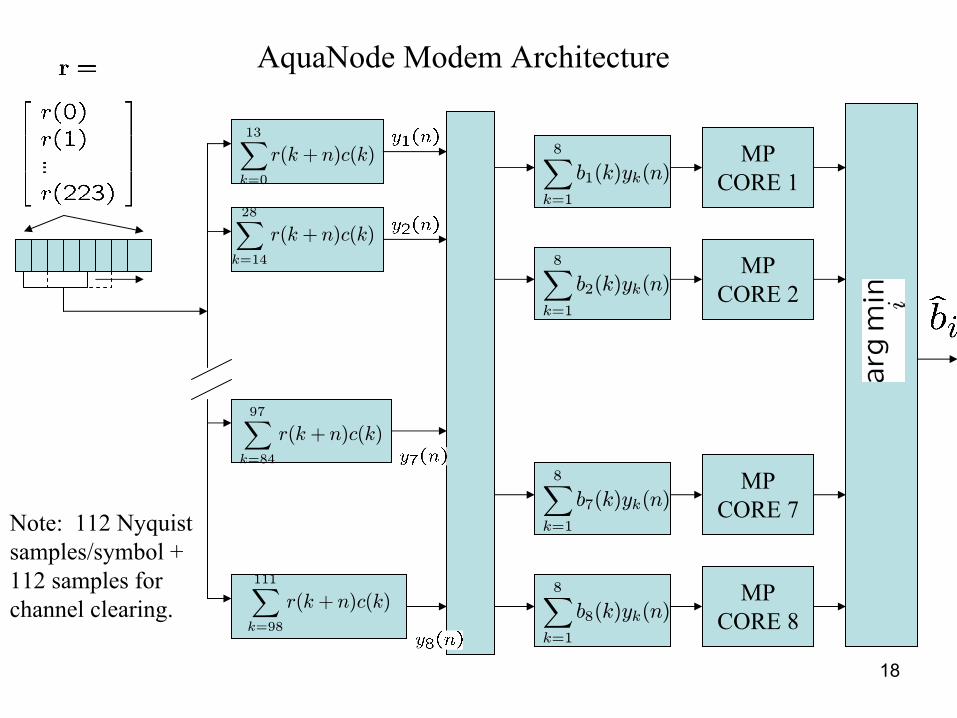
Note: 112 Nyquistsamples/symbol + 112 samples for channel clearing.
MPCORE 1
MPCORE 2
MPCORE 7
MPCORE 8
AquaNode Modem Architecture
13Xk=0
r(k+ n)c(k)
28Xk=14
r(k+ n)c(k)
111Xk=98
r(k+ n)c(k)
97Xk=84
r(k+ n)c(k)
8Xk=1
b1(k)yk(n)
8Xk=1
b2(k)yk(n)
8Xk=1
b7(k)yk(n)
8Xk=1
b8(k)yk(n)
19
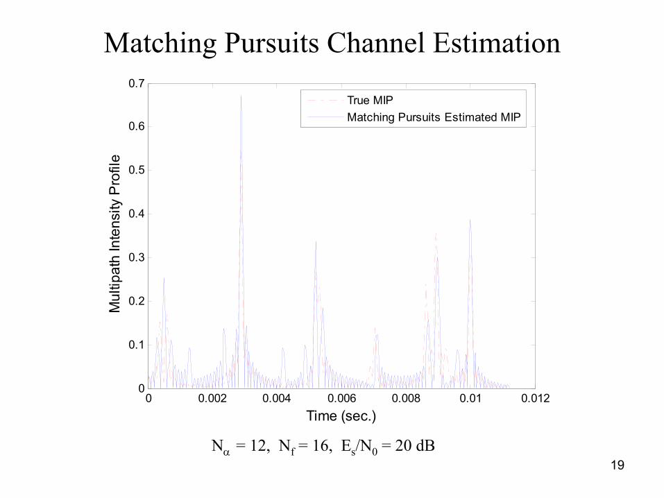
Matching Pursuits Channel Estimation
0 0.002 0.004 0.006 0.008 0.01 0.0120
0.1
0.2
0.3
0.4
0.5
0.6
0.7
Mul
tipat
h In
tens
ity P
rofil
e
Time (sec.)
True MIPMatching Pursuits Estimated MIP
Nα = 12, Nf = 16, Es/N0 = 20 dB
20
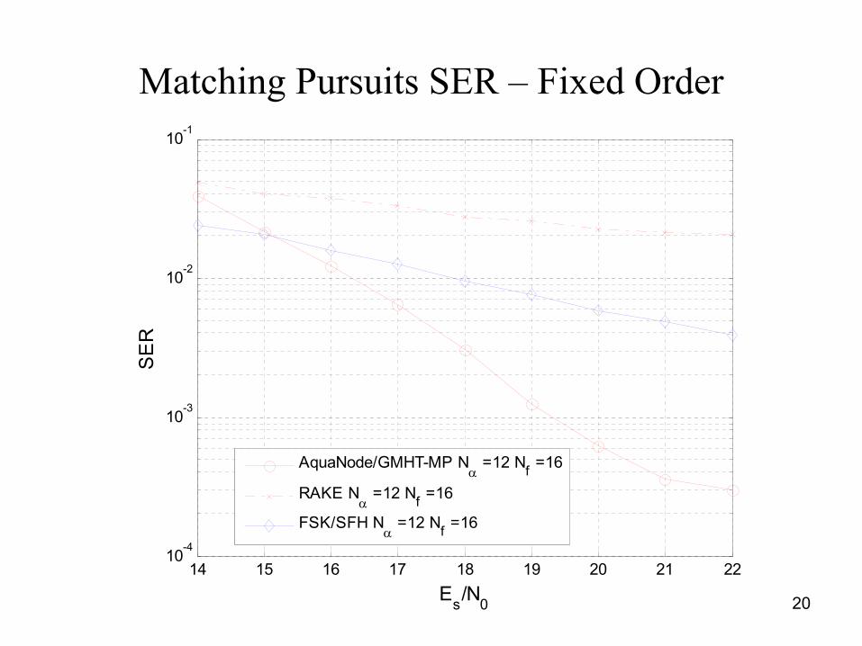
Matching Pursuits SER – Fixed Order
14 15 16 17 18 19 20 21 2210-4
10-3
10-2
10-1
Es/N0
SE
R
AquaNode/GMHT-MP Nα =12 Nf =16
RAKE Nα =12 Nf =16
FSK/SFH Nα =12 Nf =16
21
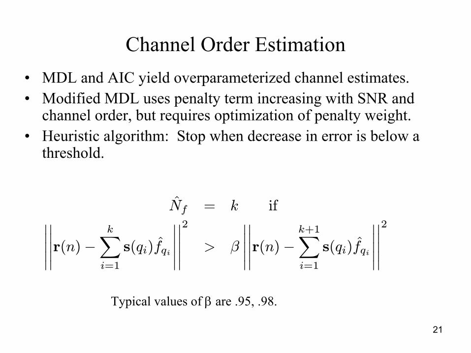
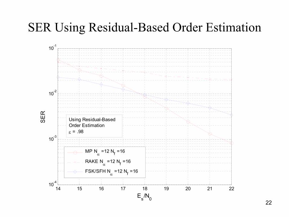
Channel Order Estimation• MDL and AIC yield overparameterized channel estimates. • Modified MDL uses penalty term increasing with SNR and
channel order, but requires optimization of penalty weight.• Heuristic algorithm: Stop when decrease in error is below a
threshold.
N̂f = k if¯̄̄̄¯¯̄̄̄¯r(n)−
kXi=1
s(qi)f̂qi
¯̄̄̄¯¯̄̄̄¯2
> β
¯̄̄̄¯¯̄̄̄¯r(n)−
k+1Xi=1
s(qi)f̂qi
¯̄̄̄¯¯̄̄̄¯2
Typical values of β are .95, .98.
22
SER Using Residual-Based Order Estimation
14 15 16 17 18 19 20 21 2210-4
10-3
10-2
10-1
Es/N0
SE
R
MP Nα =12 Nf =16
RAKE Nα =12 Nf =16
FSK/SFH Nα =12 Nf =16
Using Residual-BasedOrder Estimationε = .98
23
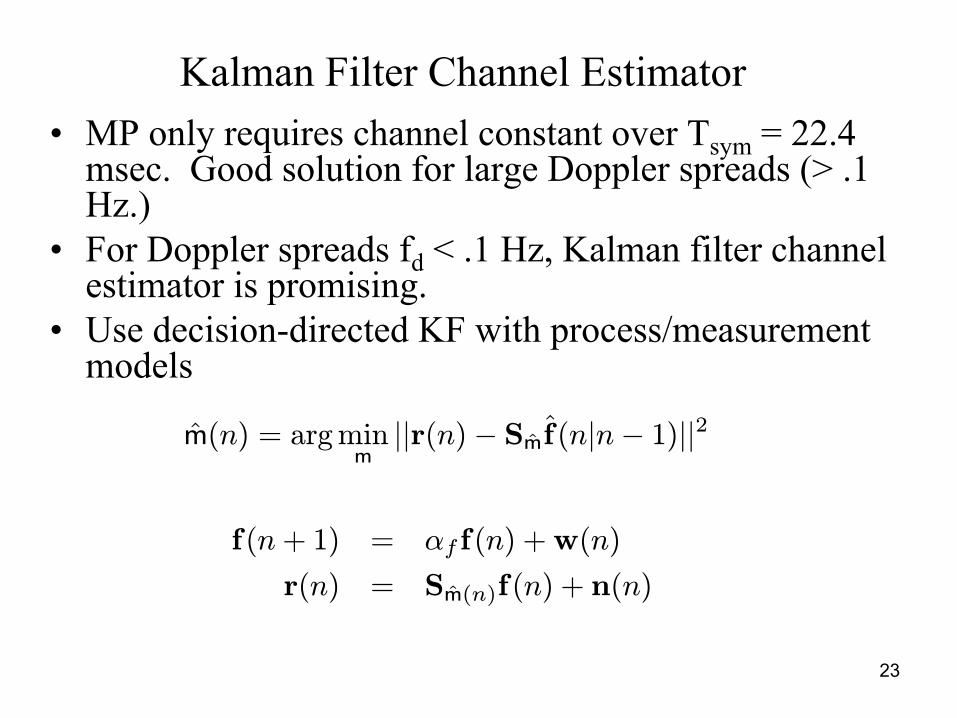
Kalman Filter Channel Estimator• MP only requires channel constant over Tsym = 22.4
msec. Good solution for large Doppler spreads (> .1 Hz.)
• For Doppler spreads fd < .1 Hz, Kalman filter channel estimator is promising.
• Use decision-directed KF with process/measurement models
f(n+ 1) = αf f(n) +w(n)
r(n) = Sm̂(n)f(n) + n(n)
m̂(n) = argminm||r(n)− Sm̂f̂(n|n− 1)||2
24
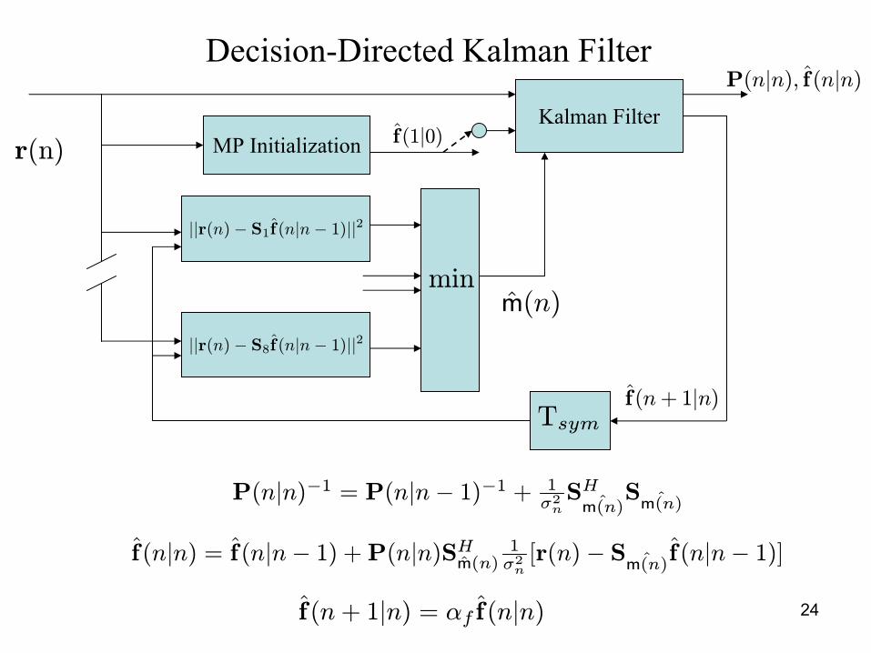
Decision-Directed Kalman Filter
r(n)
||r(n)− S1f̂ (n|n − 1)||2
||r(n)− S8f̂ (n|n − 1)||2m̂(n)
min
Kalman Filter
Tsymf̂(n+ 1|n)
f̂(n|n) = f̂(n|n− 1) +P(n|n)SHm̂(n) 1σ2n [r(n)− S ˆm(n)f̂(n|n− 1)]
P(n|n)−1 = P(n|n− 1)−1 + 1σ2nSHˆm(n)
S ˆm(n)
P(n|n), f̂(n|n)
f̂(n+ 1|n) = αf f̂(n|n)
MP Initialization f̂(1|0)
25
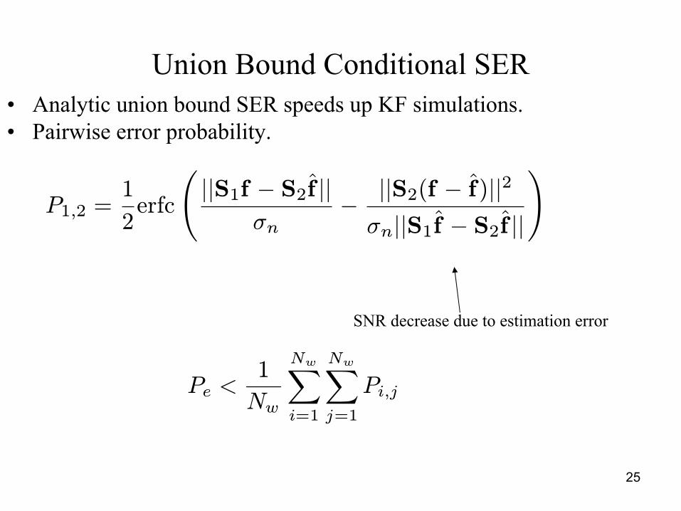
Union Bound Conditional SER• Analytic union bound SER speeds up KF simulations.• Pairwise error probability.
SNR decrease due to estimation error
P1,2 =1
2erfc
Ã||S1f − S2f̂ ||
σn− ||S2(f − f̂)||2σn||S1f̂ − S2f̂ ||
!
Pe <1
Nw
NwXi=1
NwXj=1
Pi,j
26
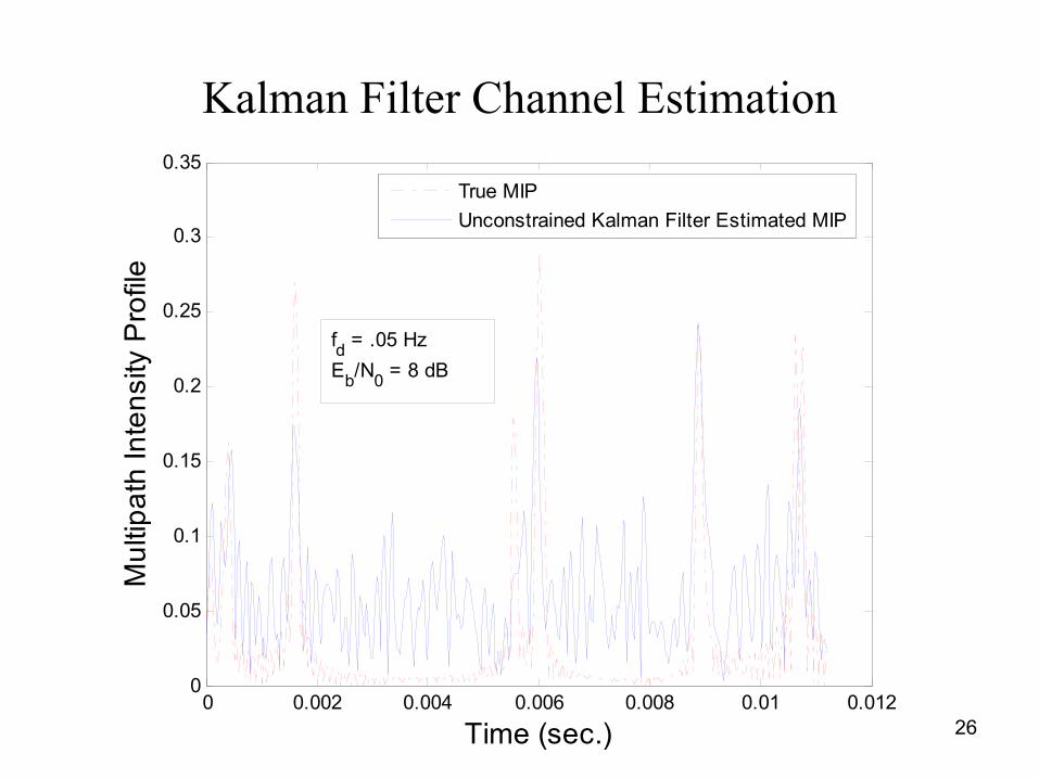
Kalman Filter Channel Estimation
0 0.002 0.004 0.006 0.008 0.01 0.0120
0.05
0.1
0.15
0.2
0.25
0.3
0.35M
ultip
ath
Inte
nsity
Pro
file
Time (sec.)
True MIPUnconstrained Kalman Filter Estimated MIP
fd = .05 HzEb/N0 = 8 dB
27
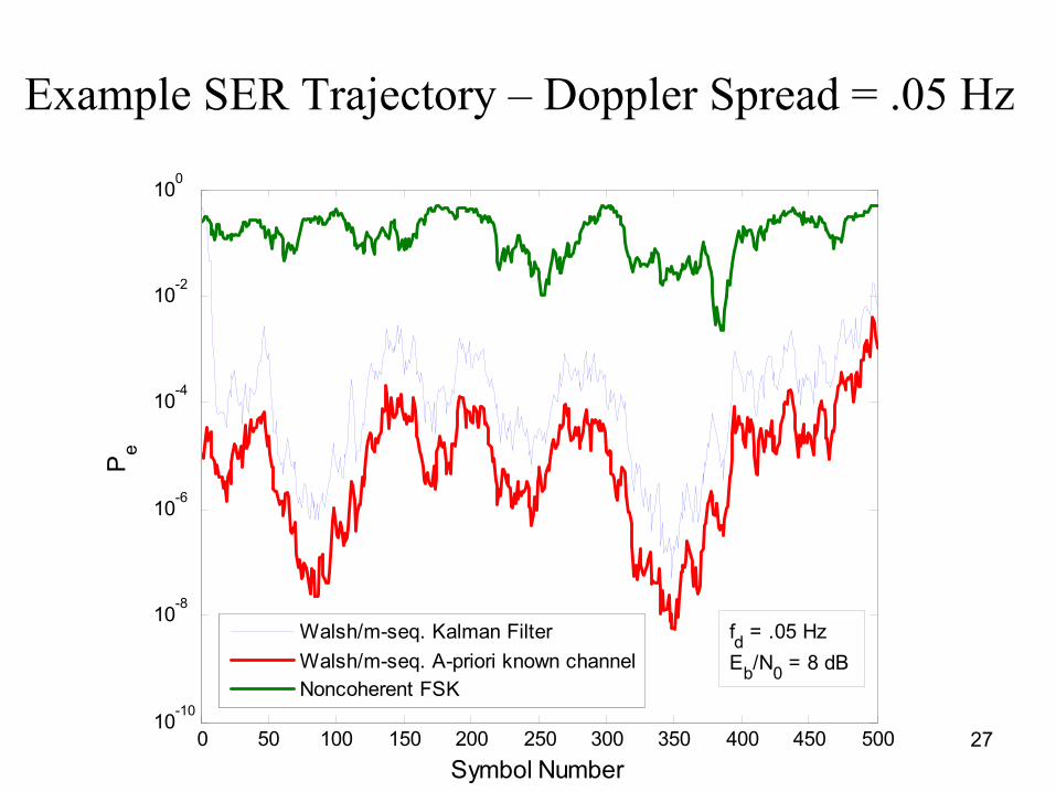
Example SER Trajectory – Doppler Spread = .05 Hz
0 50 100 150 200 250 300 350 400 450 50010-10
10-8
10-6
10-4
10-2
100
Pe
Symbol Number
Walsh/m-seq. Kalman FilterWalsh/m-seq. A-priori known channelNoncoherent FSK
fd = .05 HzEb/N0 = 8 dB
28
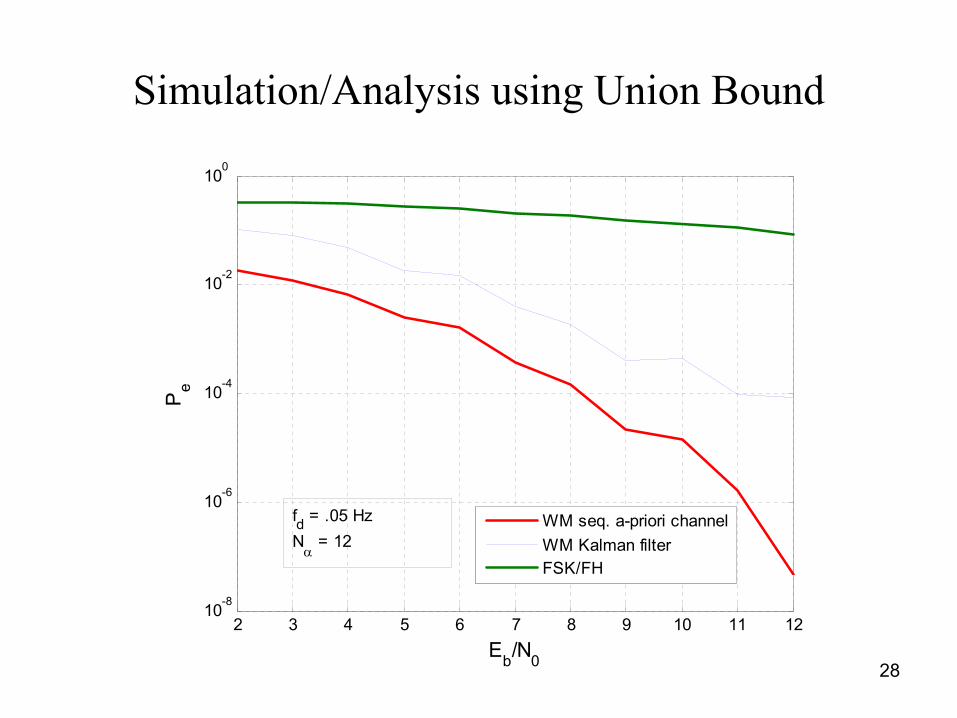
Simulation/Analysis using Union Bound
2 3 4 5 6 7 8 9 10 11 1210-8
10-6
10-4
10-2
100
Eb/N0
Pe
WM seq. a-priori channelWM Kalman filterFSK/FH
fd = .05 HzNα = 12
29
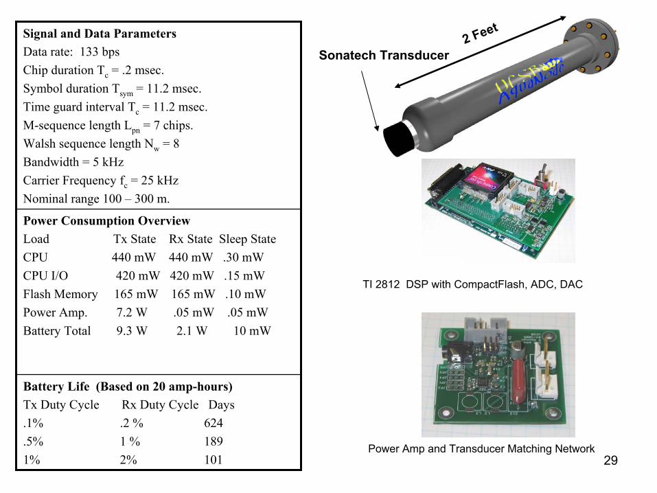
Sonatech Transducer2 Feet
Battery Life (Based on 20 amp-hours)Tx Duty Cycle Rx Duty Cycle Days.1% .2 % 624.5% 1 % 1891% 2% 101
Power Consumption OverviewLoad Tx State Rx State Sleep StateCPU 440 mW 440 mW .30 mWCPU I/O 420 mW 420 mW .15 mWFlash Memory 165 mW 165 mW .10 mWPower Amp. 7.2 W .05 mW .05 mWBattery Total 9.3 W 2.1 W 10 mW
Signal and Data ParametersData rate: 133 bpsChip duration Tc = .2 msec.Symbol duration Tsym = 11.2 msec.Time guard interval Tc = 11.2 msec.M-sequence length Lpn = 7 chips.Walsh sequence length Nw = 8Bandwidth = 5 kHzCarrier Frequency fc = 25 kHzNominal range 100 – 300 m.
Power Amp and Transducer Matching Network
TI 2812 DSP with CompactFlash, ADC, DAC
30
Conclusions
• Walsh/m-sequence signaling exploits frequency diversity and yields lower uncoded SER than FSK.
• Matching Pursuits algorithm enforces sparse estimates, implemented in FPGA and DSP.
• Modem should be adaptive, using Kalman or MP channel estimation depending on sensed channel variation, velocity.
• Can a numerosity-constrained Kalman filter be developed? Better performance for fd > .1 Hz?
• First generation modem implementable in DSP, but second gen. will require DSP +FPGA.