AN OPTIMAL SOLUTION FOR THE MULTI-AGENT

RENDEZVOUS PROBLEM APPEARING IN

COOPERATIVE CONTROL

a thesis

submitted to the department of electrical and

electronics engineering

and the institute of engineering and sciences

of bilkent university

in partial fulfillment of the requirements

for the degree of

master of science

By

Fatih Kolmek

September 2008

brought to you by COREView metadata, citation and similar papers at core.ac.uk

provided by Bilkent University Institutional Repository

I certify that I have read this thesis and that in my opinion it is fully adequate,

in scope and in quality, as a thesis for the degree of Master of Science.

Prof. Dr. Hitay Ozbay (Supervisor)

I certify that I have read this thesis and that in my opinion it is fully adequate,

in scope and in quality, as a thesis for the degree of Master of Science.

Prof. Dr. Omer Morgul

I certify that I have read this thesis and that in my opinion it is fully adequate,

in scope and in quality, as a thesis for the degree of Master of Science.

Dr. Cosku Kasnakoglu

Approved for the Institute of Engineering and Sciences:

Prof. Dr. Mehmet BarayDirector of Institute of Engineering and Sciences

ii

ABSTRACT

AN OPTIMAL SOLUTION FOR THE MULTI-AGENT

RENDEZVOUS PROBLEM APPEARING IN

COOPERATIVE CONTROL

Fatih Kolmek

M.S. in Electrical and Electronics Engineering

Supervisor: Prof. Dr. Hitay Ozbay

September 2008

The multi-agent rendezvous problem appearing in cooperative control is consid-

ered in this thesis. There are various approaches to this topic as the objectives

and problem set-ups vary in real-life rendezvous problems. Some of the applica-

tions can be given as the coordination of autonomous mobile robots or unmanned

air vehicles (UAVs) for joint tasks, and motion planning for vehicle convoys. The

problem is basically on providing a rendezvous for mobile agents at a specified

or unspecified destination. What makes the topic interesting is maintaining a

coordination between the mobile agents so that the agents reach the rendezvous

point simultaneously. Early or late arrivals are not desired.

An energy optimal solution is obtained for the problem. Imperfect road

conditions, obstacles, internal problems of the agents or similar disturbances

are also tried to be handled. As these factors are included in the problem, it

is assumed that the agents communicate between each other at specified time

instants exchanging information about their expected arrival times in order to

maintain a common rendezvous time among the team.

iii

The solution is initially derived for rendezvous in one-dimensioned space.

Then, the problem configuration is altered for two-dimensioned motions, and the

target point is assumed to be moving in order to extend the solution to possible

practical applications. The effect of increasing disturbance on the control input

and time delays in the communication are also discussed.

Keywords: Multi-Agent Rendezvous Problem, Optimal Control, Cooperative

Control, Minimum Energy Control, Calculus of Variations.

iv

OZET

ISBIRLIKLI KONTROLDE GORULEN COK ARACLI

BULUSMA PROBLEMI ICIN OPTIMAL BIR COZUM

Fatih Kolmek

Elektrik ve Elektronik Muhendisligi Bolumu Yuksek Lisans

Tez Yoneticisi: Prof. Dr. Hitay Ozbay

Eylul 2008

Bu tezde, isbirlikli kontrolde gorulen cok araclı bulusma problemi ele

alınmaktadır. Bu konuya yapılan yaklasımlar, gercek hayattaki bulusma prob-

lemlerinin amaclarının ve problem duzeneklerinin birbirlerinden farklı olması

nedeniyle cesitlilik gosterir. Problemin bazı uygulamalarına ornek olarak,

hareketli ozerk robotların veya insansız hava araclarının (IHA) birlesik gorevler

icin koordine edilmesi ve arac konvoyları icin hareket planlaması verilebilir.

Problem temel olarak, hareketli aracların belirli veya belirsiz bir varıs nok-

tasında bulusmalarının saglanmasına dayalıdır. Konuyu ilginc kılan sey,

erken veya gec varıslar istenen durumlar olmadıgından, bulusmanın aynı anda

gerceklesmesini saglayacak sekilde hareketli olan araclar arasında bir koordinasy-

onun saglanmasıdır.

Problem icin enerji acısından optimal bir cozum elde edilirken, mukemmel

olmayan yol durumlarının, engellerin, aracların icsel problemlerinin veya benzer

bozucu etkilerin de ele alınmasına calısılmaktadır. Bu etkenler probleme dahil

edildiginden, aracların takım icerisinde ortak bir bulusma zamanı belirleyebilmek

icin, birbirleri arasında muhtemel varıs zamanları hakkında bilgi alıs verisinde

bulunmak uzere haberlestikleri kabul edilmektedir.

v

Cozum baslangıcta bir boyutlu uzaydaki bulusma icin gelistirilmektedir. Son-

rasında ise, problemin konfigurasyonu iki boyutlu hareketler icin degistirilmekte

ve cozumun muhtemel pratik uygulamaları kapsayacak sekilde genisletilebilmesi

isin hedef noktasının hareket ettigi varsayılmaktadır. Ayrıca, kontrol girdisi

uzerindeki bozucu etkilerin ve haberlesmedeki zaman gecikmelerinin artması du-

rumları da tartısılmaktadır.

Anahtar Kelimeler: Cok Araclı Bulusma Problemi, Optimal Kontrol, Isbirlikli

Kontrol, Minimum Enerji Kontrolu, Degisimler Hesabı.

vi

ACKNOWLEDGMENTS

I would like to gratefully thank my supervisor Prof. Dr. Hitay Ozbay for his

guidance, support and encouragement throughout my graduate study.

I would like to thank the members of my thesis committee Prof. Dr. Omer

Morgul and Dr. Cosku Kasnakoglu for reading and commenting on this thesis.

I would like to thank my colleagues and our group head Rıza Gungor at EPDK

for their support and encouragement.

I would like to thank my family for always being by my side whenever I needed.

Finally, I would like to express my special thanks to my wife for her endless

support, encouragement, patience and understanding while writing this thesis.

vii

Contents

1 INTRODUCTION 1

1.1 Cooperative Control . . . . . . . . . . . . . . . . . . . . . . . . . 2

1.2 Optimal Control . . . . . . . . . . . . . . . . . . . . . . . . . . . 3

1.3 Rendezvous Problem . . . . . . . . . . . . . . . . . . . . . . . . . 4

1.4 Thesis Contribution and Organization . . . . . . . . . . . . . . . 8

2 PROBLEM STATEMENT AND PRELIMINARIES FROM

OPTIMAL CONTROL THEORY 9

2.1 Description of the Problem . . . . . . . . . . . . . . . . . . . . . . 9

2.2 Preliminaries from Optimal Control Theory . . . . . . . . . . . . 12

2.2.1 Calculus of Variations . . . . . . . . . . . . . . . . . . . . 12

2.2.2 Minimum Energy Control . . . . . . . . . . . . . . . . . . 18

2.3 Adaptation of the Solution to the Multi-Agent Rendezvous Problem 22

3 APPLICATION TO RENDEZVOUS PROBLEMS 25

3.1 Multi-Agent Rendezvous Problem in 1-D . . . . . . . . . . . . . . 25

viii

3.1.1 Three-Vehicle Rendezvous Problem . . . . . . . . . . . . . 26

3.1.2 Three-Vehicle Rendezvous Problem in the Presence of

Communication Problems . . . . . . . . . . . . . . . . . . 29

3.2 Multi-Agent Rendezvous Problem in 2-D . . . . . . . . . . . . . . 46

3.2.1 2-D Rendezvous Problem with Fixed Target . . . . . . . . 46

3.2.2 2-D Rendezvous Problem with Moving Target . . . . . . . 49

3.2.3 2-D Rendezvous Problem with Moving Target in the Pres-

ence of Communication Problems . . . . . . . . . . . . . . 52

3.3 Effects of Increasing Disturbance and Time Delay on the Solution 57

3.3.1 Increasing Disturbance . . . . . . . . . . . . . . . . . . . . 58

3.3.2 Increasing Time Delay . . . . . . . . . . . . . . . . . . . . 62

4 CONCLUSIONS 66

APPENDIX 68

A Matlab code for the solution of rendezvous in 1-D 68

B Matlab code for the solution of rendezvous in 2-D 71

ix

List of Figures

2.1 Rendezvous problem for N vehicles . . . . . . . . . . . . . . . . . 10

2.2 Position, velocity and control input for t0i = 0, tfi = 10 . . . . . . . 16

2.3 Position,velocity and control input for t0i = 0, tfi = 5 . . . . . . . . 16

2.4 Position, velocity and control input for t0i = 0, tfi = 3 . . . . . . . 17

2.5 Position, velocity and control input for t0i = 0, tfi = 5 in minimum

energy control . . . . . . . . . . . . . . . . . . . . . . . . . . . . . 21

2.6 Position, velocity and control input for t0i = 0, tfi = 10 in minimum

energy control . . . . . . . . . . . . . . . . . . . . . . . . . . . . . 21

2.7 Position & control inputs vs. time for t0i = 0, tfi = 10 in minimum

energy control . . . . . . . . . . . . . . . . . . . . . . . . . . . . . 24

2.8 Change in tf at communication instants for t0i = 0, tfi = 10 in

minimum energy control . . . . . . . . . . . . . . . . . . . . . . . 24

3.1 Positions vs. time for rendezvous in 1-D without communication

problems . . . . . . . . . . . . . . . . . . . . . . . . . . . . . . . . 27

3.2 Control inputs vs. time for rendezvous in 1-D without communi-

cation problems . . . . . . . . . . . . . . . . . . . . . . . . . . . . 28

x

3.3 Change in tf at communication instants for rendezvous in 1-D

without communication problems . . . . . . . . . . . . . . . . . . 28

3.4 Positions vs. time for rendezvous in 1-D with one-way time delays

in communication . . . . . . . . . . . . . . . . . . . . . . . . . . . 32

3.5 Control inputs vs. time for rendezvous in 1-D with one-way time

delays in communication . . . . . . . . . . . . . . . . . . . . . . . 33

3.6 Velocities vs. time for rendezvous in 1-D with one-way time delays

in communication . . . . . . . . . . . . . . . . . . . . . . . . . . . 34

3.7 Accelerations vs. time for rendezvous in 1-D with one-way time

delays in communication . . . . . . . . . . . . . . . . . . . . . . . 34

3.8 Change in tfi s at communication instants for rendezvous in 1-D

with one-way time delays in communication . . . . . . . . . . . . 35

3.9 Positions vs. time for rendezvous in 1-D including communication

problems . . . . . . . . . . . . . . . . . . . . . . . . . . . . . . . . 39

3.10 Control inputs vs. time for rendezvous in 1-D including commu-

nication problems . . . . . . . . . . . . . . . . . . . . . . . . . . . 39

3.11 Velocities vs. time for rendezvous in 1-D including communication

problems . . . . . . . . . . . . . . . . . . . . . . . . . . . . . . . . 40

3.12 Accelerations vs. time for rendezvous in 1-D including communi-

cation problems . . . . . . . . . . . . . . . . . . . . . . . . . . . . 40

3.13 Change in tfi s at communication instants for rendezvous in 1-D

including communication problems . . . . . . . . . . . . . . . . . 41

3.14 Positions vs. time for rendezvous in 1-D including communication

problems . . . . . . . . . . . . . . . . . . . . . . . . . . . . . . . . 43

xi

3.15 Control inputs vs. time for rendezvous in 1-D including commu-

nication problems . . . . . . . . . . . . . . . . . . . . . . . . . . . 44

3.16 Velocities vs. time for rendezvous in 1-D including communication

problems . . . . . . . . . . . . . . . . . . . . . . . . . . . . . . . . 44

3.17 Accelerations vs. time for rendezvous in 1-D including communi-

cation problems . . . . . . . . . . . . . . . . . . . . . . . . . . . . 45

3.18 Change in tfi s at communication instants for rendezvous in 1-D

including communication problems . . . . . . . . . . . . . . . . . 45

3.19 Position trajectories for rendezvous in 2-D with fixed target . . . 48

3.20 Velocities vs. time for rendezvous in 2-D with fixed target . . . . 48

3.21 Position trajectories for rendezvous in 2-D with moving target . . 51

3.22 Velocities vs. time for rendezvous in 2-D with moving target . . . 51

3.23 Position trajectories for rendezvous in 2-D with moving target . . 53

3.24 Velocities vs. time for rendezvous in 2-D with moving target . . . 54

3.25 Change in tfi s at communication instants for rendezvous in 2-D

with moving target . . . . . . . . . . . . . . . . . . . . . . . . . . 54

3.26 Position trajectories for rendezvous in 2-D with moving target

including communication problems . . . . . . . . . . . . . . . . . 56

3.27 Velocities vs. time for rendezvous in 2-D with moving target in-

cluding communication problems . . . . . . . . . . . . . . . . . . 56

3.28 Change in tfi s at communication instants for rendezvous in 2-D

with moving target including communication problems . . . . . . 57

xii

3.29 Position trajectories for increasing disturbances . . . . . . . . . . 59

3.30 Magnitudes of the control inputs vs. time for increasing disturbances 60

3.31 Final times vs. time for increasing disturbances . . . . . . . . . . 61

3.32 Position trajectories for increasing time delay in the communication 63

3.33 Magnitudes of the control inputs vs. time for increasing time delay

in the communication . . . . . . . . . . . . . . . . . . . . . . . . . 64

3.34 Final times vs. time for increasing time delay in the communication 65

xiii

List of Tables

3.1 Calculated Final Time tf w.r.t. the communication instant . . . . 30

3.2 Final Times in the absence of time delays hiks . . . . . . . . . . . 30

3.3 Communication delays hik in sec. for corresponding instants k . . 31

3.4 Final Times in the presence of time delays hiks . . . . . . . . . . . 31

3.5 Calculated Final Times tfi (k) w.r.t. the communication instant . . 36

3.6 Final Times in the absence of time delays hij(k)s . . . . . . . . . 37

3.7 Final Times in the presence of time delays hij(k)s . . . . . . . . . 38

3.8 Calculated Final Times tfi (k) w.r.t. the communication instant . . 41

3.9 Final Times in the absence of time delays hij(k)s . . . . . . . . . 42

3.10 Final Times in the presence of time delays hij(k)s . . . . . . . . . 43

xiv

to mom and dad . . .

Anneme ve babama . . .

Chapter 1

INTRODUCTION

In this thesis, we investigate optimal solutions for a rendezvous problem appear-

ing in cooperative control. The problem in question is getting N > 1 vehicles in

a task force to reach a specified point at the same time instant. It is assumed

that these vehicles communicate with each other exchanging information about

their expected final time to reach the rendezvous point in order to avoid early or

late arrivals, and this communication occurs at discrete time instants.

The interesting part of the problem is that the final times of the vehicles

may change during the mission due to unforeseen events, like obstacles on the

road or internal problems of the vehicles, and there might be time delays in the

communication between the vehicles. Therefore, a satisfactory solution for the

stated rendezvous problem should take these conditions into account and provide

reliable results in order to be applicable.

Before attacking the problem, let us give some information about the concepts

related with the subject and present a brief information about the similar studies

in the literature.

1

1.1 Cooperative Control

Research on control of multi-vehicle systems performing cooperative tasks gained

importance in the late 1980s [1] when several researchers began investigations in

multiple mobile robot systems [2]. Since then, the interest in this topic has

increased significantly thanks to the development of inexpensive and reliable

wireless communications systems and the application fields in military operations

[1].

The most popular problems of cooperative control of mobile robots involve

groups or teams of autonomous vehicles cooperating to complete a mission [3].

Basically, the success of the mission can only be attained when none of the

vehicles or groups that are performing separate tasks fail, i.e. each individual

performing the corresponding task must succeed. The interesting part of the

problem is that the vehicles or the groups have to perform coordinated actions [3]

in order to complete their individual tasks.

At this point, it is helpful to give a concise explanation about what is meant by

cooperative control before going into more detail in the subject. A comprehensive

study about the recent researches on the topic can be found in [1].

Consider a group of vehicles aiming to complete a task and the corresponding

overall performance function below.

J =

∫ T

0

L(x, α, u)dt + V (x(T ), α(T )) (1.1)

where x is the states, α is the roles, T is the final time that the task should be

completed, L is the incremental cost of the task and V represents the terminal

cost of the task. Notice that (1.1) is a typical cost function.

A task is called decoupled, if the cost function J can be written as

2

J =N∑

i=0

(∫ T

0

Li(xi(t), αi(t), ui(t))dt + V i(xi(T ), αi(T ))

)(1.2)

where

i : the index corresponding to vehicle i

xi(t) : the state of vehicle i at time t

αi(t) : the role of vehicle i at time t that is

subject to change during the task

ui(t) : the input controlling the state of vehicle i at time t

xi(T ) : the final value of the state of vehicle i

αi(T ) : the final value of the role of vehicle i

otherwise, the task is called coupled or namely cooperative which means that

the task performance depends on the joint locations, roles and inputs of the

vehicles [1].

Then, cooperative control can simply be defined as determining the control

law ( i.e. the control input ui(t)) that solves the coupled performance function

which is the dual of (1.2) corresponding to a cooperative task defined above.

1.2 Optimal Control

Optimal control can basically be described as the problem of determining a con-

trol law for a given system while satisfying the specified optimality conditions.

A precise mathematical description can be given as finding an admissible control

u∗(t) which forces the following system with x(t) as the state, u(t) as the control

input and t is time

3

x(t) = f (x(t), u(t), t) (1.3)

to follow an admissible trajectory x∗(t) that minimizes or maximizes the perfor-

mance measure in the form

J = h(x(tf ), tf ) +

∫ tf

t0

g(x(t), u(t), t)dt (1.4)

with u∗(t) being the optimal control input and x∗(t) being the optimal trajectory

[4]. Here, f, g, h are specified functions that satisfy certain assumptions, see

e.g. [4].

In this study, the solutions for the multi-agent rendezvous problem are to

be optimal with constraints like fixed initial and final states, and the cost to be

minimized is the control energy. Therefore, we will form a performance measure

as in (1.4) that involves the constraints to be considered, and solve for the optimal

input resulting in a successful rendezvous.

1.3 Rendezvous Problem

The multi-agent rendezvous problem in this thesis is an optimal control problem

appearing in cooperative control. The idea is having a number of mobile agents

arrive at a meeting point, namely the rendezvous point, at the same time. The

crucial point is assuring that the agents perform cooperative actions by arranging

themselves according to the information gathered from the other agents in the

team [5].

Actually, the title “rendezvous problem” is a broad one, and it is a general

name for various problems in cooperative control some of which are;

4

� The problem of two aircrafts aiming to meet at a non-specified point at a

predefined final time [6],

� The problem of trajectory planning for the vehicles in a team aiming to

reach the neighborhood of a point not before the other vehicles in the

team [7],

� The problem of path planning for a robot aiming to reach a target [8, 9],

� The coordination of unmanned aerospace vehicles (UAVs) to reach a target

point [10],

� The problem of enabling mobile users in a location, tracking and rendezvous

with a variety of mobile entities [11],

� The problem of conflict management in a multi-user computer network [12],

� The problem of motion planning for vehicle convoys [13],

� The problem of multi-agent rendezvous [14–17],

Probably, the most popular one of the problems above is the multi-agent

rendezvous problem which is the subject discussed in this thesis. The popularity

is basically due to variety of applications in military operations ranging from

cooperative attack in land operations to cooperative control of unmanned air

vehicles (UAVs) for rendezvous in air operations. In the literature there are many

versions of this problem involving constraints such as rendezvous with fixed final

time, time optimal rendezvous with unspecified final states, and energy efficient

rendezvous. Next, some of the solutions to similar rendezvous problems are

presented.

In one of the studies related with the multi-agent rendezvous, the problem

of determining a meeting point while minimum energy consumption is taken

into account is discussed [18]. In that paper, a multi-robot team, which consists

5

of autonomous mobile robots trying to meet at a single point for a mission, is

considered, and two solutions about the minimum energy consumption during

the travels towards the rendezvous point are proposed. The interesting part of

the problem is that the cost of travel for each robot is different and the goal is to

find an energy efficient solution considering the robots in the team as a whole.

Although the proposed solutions are successful in finding a rendezvous point,

the proposed algorithms do not consider a timing constraint. In addition, as

indicated in the paper, the solutions assume a reliable communication between

the robots, and communication delays or loss of information about the current

positions of the robots are not handled.

A similar problem on multi-agent rendezvous is considered in [15,16]. In that

setting, there are N > 1 vehicles aiming to meet at an unspecified point which is

regarded as rendezvous by sensing the current positions of the neighboring mobile

agents that are within their sensing region. The presented solution is basically

determining decentralized control algorithms for the agents. In other words, the

solution just guarantees the rendezvous for the agents but does not include the

constraints on the control energy, the final states (velocity and acceleration) of

the agents, and imperfect communication.

Another related study about the multi-agent rendezvous problem is on the

stability of mobile robot rendezvous [8]. In this study, a mobile robot aiming

to reach a target point is considered, and an optimal control is derived. In that

problem, the destination point and the final time is specified for an autonomous

robot, and the robot aims to arrive the rendezvous point on time while evaluat-

ing its current states with respect to the rendezvous point and arranging itself

accordingly via applying a step control acceleration. Both 1-D and 2-D solutions

are provided assuming that the states are known and there is no noise or distur-

bance in the system. Besides, the solutions are derived for a single autonomous

robot and thus exclude a cooperative control scheme and communication with

6

a central point or any other agent. Moreover, the resulting control inputs have

large magnitudes and there is a possibility of instability as the robots gets closer

to the rendezvous point, for that reason a limit is placed on the applied control

input.

A very similar work is presented in [19] in which a multi-robot rendezvous

problem is discussed. The goal of the problem is to determine control laws for

N robots moving in the horizontal plane in order to reach a moving robot at

the same time. The motion of the moving robot, namely the reference-robot is

not a priori known by other robots aiming to catch it. It is assumed that all

robots move faster than the reference robot, the motion of the reference robot

is continuous and there is a reliable communication between the leader robot

and the others, and a sensory system in order to determine the position of the

reference robot. In that paper two approaches for the solution are presented.

� First one is the leader-follower approach in which the leader of the team

tracks the position of the reference robot and the team members try to

follow the leader. Since the leader perfectly tracks the reference-robot and

the others catch the leader eventually, all the robots catch the reference

robot consequently. In that approach, it is also assumed that the followers

move faster than their leader.

� The second one is the reference-robot approach in which all the robots

sense the position of the reference robot continuously and try to catch it.

Since all the robots move faster than the reference robots, all the robots in

the team catches the reference-robot successfully.

The solutions are obtained via relative kinematic equations and they are suc-

cessful as all the robots catch the reference-robot at the same time. However,

7

the solutions include neither time nor energy optimality constraints, and it is as-

sumed that there is no communication deficiency like lost or delayed information

signals between the robots.

1.4 Thesis Contribution and Organization

In the following chapters, the multi-agent rendezvous problem in question is

described, the mathematical solution is derived and the application results are

presented. The major advantage of the solutions given here is being optimal in

terms of the control energy used by the mobile agents while providing a suc-

cessful rendezvous with pre-specified initial and final states. Moreover, delayed

communication for simultaneous cooperative rendezvous is handled.

Remaining parts of the thesis are organized as follows. In Chapter 2, the

configuration of the multi-agent rendezvous problem is described and the basics of

the mathematical solution are introduced together with some simple illustrative

examples. The application of the solution to the problem is given in Chapter 3.

The solutions for rendezvous in 1-D in the presence/absence of communication

problems modeling delayed or lost information about the estimated times of

arrivals are presented. The solution is extended to 2-D and the case of moving

target point is addressed for practical applications. The effect of increasing

disturbance on the control input and time delays in the communication are also

discussed. Chapter 4 includes the conclusions and some notes about possible

complementary studies to be made.

8

Chapter 2

PROBLEM STATEMENT AND

PRELIMINARIES FROM

OPTIMAL CONTROL

THEORY

In this chapter, the description of the multi-agent rendezvous problem is given.

Basic concepts and tools from optimal control theory are described in order to

establish a background for the problem solution.

2.1 Description of the Problem

As stated in the introduction briefly, we will discuss a rendezvous problem ap-

pearing in cooperative control. Remember that there are N > 1 vehicles in a

task force and their goal is to reach a target point(rendezvous point) at the same

time instant spending as low energy as possible. It is assumed that they com-

municate with each other at specified time instants during their mission in order

9

to arrange their states so that they all arrive the target point at the same time

instant, neither before nor after.

Consider the rendezvous problem for N vehicles illustrated in Figure 2.1.

The vehicles aim to reach the target point pt at the same time instant. Basically,

one can assign a final time tf for the mission and inform the vehicles to be

at the target point at time tf and the vehicles arrange their acceleration or

velocity accordingly. However, if one of the vehicles fails to be at pt at time

tf due to an internal problem or bad road conditions, the mission may not be

completed successfully. In order to overcome that problem, it is better to utilize

an information exchange between the vehicles about their position, velocity and

acceleration or just the estimated time of arrival at discrete time instants. Thus,

at each information exchange instant the vehicles can use the information that

they received from the other vehicles in the team as a feedback to arrange their

states and try to catch the fastest or the slowest of the team in order to arrive

the rendez-vous point pt at the same instant.

Figure 2.1: Rendezvous problem for N vehicles

10

Consider the following dynamical model for the vehicles

xi(t) = f(xi(t), ui(t), wi(t)) (2.1)

where f is a known function of the state xi, input ui and the disturbance wi. The

state xi consists of the position, velocity and the acceleration of the ith vehicle

in space. In order to simplify the problem we may consider the following linear

case assuming that wi(t) = 0:

xi(t) = Aixi(t) + Biui(t) (2.2)

where Ai =

0 1 0

0 0 1

0 0 0

, Bi =

0

0

1

. The target point is assumed be fixed

at the origin. In order to determine the solution guaranteeing the success of the

mission, the following quadratic cost function should be solved for the minimizing

optimal control input ui(t):

Ji(t) =

∫ tfi

t

(‖xi(τ)‖2Qi

+ ‖ui(τ)‖2Ri

)dτ + ‖xi(tfi )‖Qf

i(2.3)

where Qi, Ri and Qfi are the weighting matrices of appropriate dimensions. What

makes the problem interesting is that in the equation above, the final time tfi

is time varying, and is updated at discrete time instants tk depending on the

feedback received from the other vehicles. There are two choices:

tfi (t) = min{t1f (t), t2f (t), t3f (t), . . . , tNf (t)} (2.4)

or

tfi (t) = max{t1f (t), t2f (t), t3f (t), . . . , tNf (t)} (2.5)

where tjf (t) is the expected time of arrival for the jth vehicle at time t, and is a

function of position, velocity, acceleration and control input of the jth vehicle.

11

We can denote tjf (t) as tjf (t) = p(xjp(t), vjp(t), ajp(t), uj(t)), where xjp(t),

xjv(t), xja(t) and uj(t) are the position, velocity, acceleration and control input

of the jth vehicle at time t, respectively. Here, p is a function to determine the

final time of a vehicle by assuming that current optimal control input u∗i (t) will

not be subject to any change during the rest of the travel. Note that, tfi (t) is

generated from a data set of N received by the ith vehicle up to time t. In order

to have a more realistic problem, it is convenient to assume that there are time

delays in the communications between each vehicle, i.e.:

tfi (t) = min{t1f (t−h1i(t)), tf2(t−h2i(t)), t

f3(t−h3i(t)), . . . , t

fN(t−hNi(t))} (2.6)

or

tfi (t) = max{tf1(t− h1i(t)), tf2(t− h2i(t)), t

f3(t− h3i(t)), . . . , t

fN(t− hNi(t))} (2.7)

where hji(t) represents the time delay in the one way communication from vehicle

j to vehicle i at time instant t.

2.2 Preliminaries from Optimal Control Theory

In this section the solution of the rendezvous problem described in Section 2.1 is

presented using basic principles from optimal control theory. For the time being,

suppose that the information exchange between the vehicles is perfect and not

effected by the delay. Then, we can proceed with the solution of the quadratic

cost function minimization problem.

2.2.1 Calculus of Variations

Suppose that the state xi(t) is composed of position and velocity of the ith vehicle

only, i.e.

Ai =

0 1

0 0

, Bi =

0

1

(2.8)

12

where Qi = I2×2, Ri = I2×1, Qfi = I2×2 and the initial and the final conditions

xi0 and xif are known.

Optimal solution of the quadratic cost function minimization problem defined

by (2.3) can be obtained by “Calculus of Variations” which is a well-known

method for solving optimal control problems. As explained in [4], the necessary

conditions for optimality in order to solve the problem are:

x∗i =∂H∂p

(x∗i (t), u∗i (t), p

∗i (t), t)

p∗i =∂H∂x

(x∗i (t), u∗i (t), p

∗i (t), t)

0 =∂H∂ui

(x∗i (t), u∗i (t), p

∗i (t), t) (2.9)

for all t ∈ [t0, tf ], where H is the Hamiltonian defined as

H(x(t), u(t), p(t), t) , g(x(t), u(t), t) + pT (t) [f(x(t), u(t), t)] (2.10)

and

[∂h

∂x(x∗(tf )− p∗(tf ))

]T

∂xf +

[H(x∗(tf ), p∗(tf ), tf ) +

∂h

∂t(x∗(tf ), tf )

]∂tf = 0 (2.11)

for the system and the cost function below

xi(t) = f(xi(t), ui(t), t) (2.12)

J(u) = h(x(tf ), tf ) +

∫ tf

t0

g(x(t), u(t), t)dt (2.13)

At this point, it is not difficult to construct an analogy between (2.3) and

(2.13) as follows

h(x(tf ), t) = ‖xi(Tfi (t))‖Qf

i

g(x(tf ), t) = ‖xi(τ)‖2Qi‖+ ‖ui(τ)‖2

Ri(2.14)

13

In (2.11), p∗(t) represents the Lagrange multipliers p∗1(t), p∗1(t), . . . , p

∗n(t)

which are selected as follows.

p∗(t) = −[∂f

∂x(x∗(t), u∗(t), t)

]T

p∗(t)−[∂g

∂x(x∗(t), u∗(t), t)

](2.15)

Note that, p(t) is also called costate and the equation above is called costate

equations. By solving the equations (2.9) and (2.11), the costates, the optimal

control input and the output trajectory can be obtained easily.

If we apply (2.9)-(2.15) to our simplified problem, we can have the following

formulation [4].

The Hamiltonian for the problem is

H(x(t), ui(t), pi(t), t) =1

2xT Qixi(t) +

1

2uT Riui(t) +

pT Aix(t) + pTi (t)Biui(t) (2.16)

Then, the necessary conditions for the solution in order to exist are

x∗i = Aix∗i (t) + Biu

∗i (t) (2.17)

p∗i =∂H∂xi

= −Qix∗i (t)− AT

i p∗i (t) (2.18)

0 =∂H∂u

= Riu∗i (t) + BT

i p∗i (t) (2.19)

Notice that the optimal control input ui(t) can be obtained from (2.19) as

u∗i (t) = −R−1i BT

i p∗i (t) (2.20)

Substituting (2.20) into (2.17) yields

x∗i (t) = Aix∗(t)−BiR

−1i BT

i p∗i (t) (2.21)

14

Combining (2.21) and (2.18) we have 2n linear differential equations which

are formulated below.

x∗i (t)

p∗i (t)

=

Ai

−Qi

−BiR−1i BT

i

−ATi

x∗i (t)

p∗i (t)

x∗i (t)

p∗i (t)

= Φ

x∗i (t)

p∗i (t)

(2.22)

where Φ is the transition matrix. In order to solve (2.22) we need 2n boundary

conditions, and we already have them as xi(t0) = x0i and xi(tf ) = xf

i . The rest

of the solution in order to determine the Lagrange multipliers p∗i (t), the control

input u∗i (t) and the states x∗i (t) is trivial and can be obtained easily after solving

(2.22) for x∗i (t) and p∗i (t) by following the steps explained in [20]. Remember

that the solution of a set of the 2n linear differential equations will be in the

form below x∗i (t)

p∗i (t)

= c1e

λ1tv1 + c2eλntv2t + . . . + cne

λntvn (2.23)

where cis are the coefficients, and λis and vis are the eigenvalues and the eigen-

vectors of Φ, respectively. Now, let us look at some sample results obtained by

the explained method.

The solutions for x0i =

5

0

, xf

i =

0

0

, t0i = 0, tfi = 10 and tfi = 5 are

depicted in Figures 2.2 and 2.3, respectively. In that figures, it can be observed

that the optimal control input u∗i (t) for the cost function in (2.3) brings the

vehicle to the rendezvous point at nearly t = 5 whereas the rendezvous time was

specified as tfi = 10 initially, and no change were made during the travel.

15

0 1 2 3 4 5 6 7 8 9 10−6

−4

−2

0

2

4

6

time

outp

ut

PositionVelocityControl Input

Figure 2.2: Position, velocity and control input for t0i = 0, tfi = 10

0 0.5 1 1.5 2 2.5 3 3.5 4 4.5 5−6

−4

−2

0

2

4

6

time

outp

ut

PositionVelocityControl Input

Figure 2.3: Position,velocity and control input for t0i = 0, tfi = 5

16

This result is basically due to the configuration of the cost function, because

the optimal control input is determined by taking the constraints for the control

energy and the difference between the current and final states to be reached into

account directly. In other words, the control input tries to bring the vehicle

to the rendezvous point just on time using minimum control energy but it also

forces the states to converge to zero as soon as possible. Thus, we observe that

the vehicle reaches the target point much before the specified time.

Moreover, as seen below for x0i =

5

0

, xf

i =

0

0

, t0i = 0 and tfi = 3,

if the specified final time is close to the departure time (i.e. the travel time is

short) the control input grows too much, and such a case is not acceptable due

to the practical limits of the controller. Therefore, a realizable solution is needed

and the next section addresses this problem.

0 0.5 1 1.5 2 2.5 3−6

−4

−2

0

2

4

6

time

outp

ut

PositionVelocityControl Input

Figure 2.4: Position, velocity and control input for t0i = 0, tfi = 3

17

2.2.2 Minimum Energy Control

Regarding the results obtained by solving the cost function in (2.3), it can be

concluded that the obtained control input does not solve the problem appropri-

ately due to the constraints included in cost function. Having known the reasons,

it might be possible to improve the solution.

For instance, the term ‖xi(tfi )‖Qf

ihas no relevance with the minimization of

the control input to be used since xfi = 0, and it can be excluded. Moreover,

including the term ‖xi(t)‖2Qi

in the cost function to be minimized results in a

struggle for an early arrival to the rendezvous point (i.e. tfi ) and consequently

the usage of more energy in the control input. So, we may also exclude that term

in the cost function and have the new cost function to be minimized as follows.

Ji(t) =1

2

∫ tfi

t0i

(‖ui(t)‖2Ri

)dt (2.24)

Now, the question is “How can we guarantee that the vehicle reaches the

rendezvous point having excluded the states in the cost function?” and the

answer is simple. The control input and the states are related by the system

equation in (2.2) with Ai and Bi as in (2.8). Therefore, although the term

related with the states is not involved in (2.24), the optimal solution of (2.24)

gives not only the minimum energy signal (i.e. the control input ui(t)) but also

the desired state trajectory since the solution is based on the time constraint of

t0i and tfi , and the boundary conditions of xi(t0i ) = x0

i and xi(tfi ) = xf

i . Thus,

we will solve another cost function minimization problem known as “Minimum

Energy Control Problem”.

Solution of the minimum energy control problem is based on “Calculus of

Variations Method” and basically aims to minimize the control energy in the

18

cost function of (2.24). Thus, it is expected that the optimal control input will

not grow much enabling the vehicle to reach the target point just on time.

As minimum energy control control is a very well known issue, the lengthy

derivation of the optimal control input and the minimum cost can be found

in many books like [21], [6] and [4]. Here, the derivation is skipped and only

the solution is presented, however the reader is referred to [21] for a detailed

derivation with a comprehensive explanation on the topic.

Notice that the controllability Gramian for the system in (2.2) with Ai and

Bi as in (2.8)

Wc(t0i , t

fi ) =

∫ tfi

t0i

eAi(t0i−τ)BiB

Ti eAT

i (t0i−τ)dτ (2.25)

is nonsingular for any tfi > t0i since (Ai, Bi) is a controllable pair. Then, the

minimum energy control signal ui(t) can be obtained as

u∗i (t) = −BTi eAT

i (t0i−t)W−1c (t0i , t

fi )(x

0i − eAi(t

0i−tfi )xf

i ) (2.26)

Alternatively, the minimum energy control signal can be written in terms of

the reachability Gramian Wr as

Wr(t0i , t

fi ) =

∫ tfi

t0i

eAi(tfi −τ)BiB

Ti eAT

i (tfi −τ)dτ (2.27)

and

u∗i (t) = −BTi eAT

i (tfi −t)W−1r (t0i , t

fi )(x

fi − eAi(t

fi −t0i )x0

i ) (2.28)

19

Then, the minimum energy value J∗i can be determined as

J∗i =1

2

∫ tfi

t0i

‖u∗i (t)‖2dt

=1

2(x0

i − eAi(t0i−tfi )xf

i )T W−1

c (t0i , tfi )(x

0i − eAi(t

0i−tfi )xf

i ) (2.29)

For the controllable pair (Ai, Bi) in (2.8) and the boundary conditions x0i =

5

0

and xf

i =

0

0

with t0i = 0 and tfi = 5, Wc and u∗i (t) are calculated as

Wc(t0i , t

fi ) =

13(tfi − t0i )

3 − 12(tfi − t0i )

2

−12(tfi − t0i )

2 (tfi − t0i )

=

1253

− 252

−252

53

u∗i (t) =12

25t− 6

5(2.30)

Then, the trajectory of xi(t) can easily be calculated as

x∗i (t) = eAi(t−t0i ) +

225

t3 − 35t2

625

t2 − 65t

=

1 5

0 1

5

0

+

225

t3 − 35t2

625

t2 − 65t

=

5

0

+

225

t3 − 35t2

625

t2 − 65t

(2.31)

which is plotted in Figure 2.5.

The optimal solution for tfi = 10 is also plotted in Figure 2.6. Comparing

Figures 2.2 and 2.3 with Figures 2.5 and 2.6, one can observe that the minimum

energy control solution provides the desired rendezvous results unlike the former

one.

20

0 0.5 1 1.5 2 2.5 3 3.5 4 4.5 5−2

−1

0

1

2

3

4

5

time

outp

ut

PositionVelocityControl Input

Figure 2.5: Position, velocity and control input for t0i = 0, tfi = 5 in minimum

energy control

0 1 2 3 4 5 6 7 8 9 10−1

0

1

2

3

4

5

time

outp

ut

PositionVelocityControl Input

Figure 2.6: Position, velocity and control input for t0i = 0, tfi = 10 in minimum

energy control

21

2.3 Adaptation of the Solution to the Multi-

Agent Rendezvous Problem

Up to this point, the solution was for the optimal control of one vehicle, and

now the question is: “How can we include other vehicles in the team and the

communication between them in order to update the rendezvous instant and get

all of the vehicles to be at the target point just at the rendezvous time?” The

answer is discussed next.

Remember that the optimal solution of the rendezvous problem is u∗i (t) which

minimizes the cost function in (2.24) with respect to the boundary conditions

(i.e. the initial and the final states). Now, suppose that the vehicles communicate

at each discrete time instant tk and the rendezvous time is updated or remain

unchanged with respect to the received information. Then, we can solve for u∗i (t)

by accepting x0i as the value of the states at the communication instant and xf

i

as the value of the states at the rendezvous instant.

Knowing the exact values of the states at the communication instant and the

required distance to be traveled, it is not so difficult to solve for tfnew

i which is

the new rendezvous time for vehicle i. In order to determine tfnew

i at time tk, it

is assumed that the current optimal control input u∗i (t) will not change during

the rest of the travel. That means the trajectory of the ith vehicle’s position will

remain the same during the rest of the travel. As seen in (2.31), the trajectory

of the position of vehicle i (i.e. xip(t)) is a third order polynomial of t. Similarly,

xip(t) will be a fifth order polynomial of t when we include the acceleration in

our model. So, we can express xip(t) as

xip(t) = antn + an−1t

n−1 + an−2tn−2 + . . . + a1t + a0 (2.32)

22

Then, we can express the distance to be traveled by vehicle i as

xfip − x0

ip = ∆xip

= an(tfnew

i )n + an−1(tfnew

i )n−1 + . . . + a1tfnew

i −(an(tk)

n + an−1(tk)n−1 + . . . + a1(tk)

)(2.33)

in order to determine tfnew

i . Here, x0ip and xf

ip are the positions of vehicle i at

the communication instant tk and the rendezvous time, respectively. We can

determine the coefficients an, an−1, . . . , a1 at the communication instant by using

the previous values of xip. Then, we can solve (2.33) for tfnew

i and determine the

new rendezvous time for vehicle i.

By repeating this procedure at the communication instants, each vehicle can

determine its own expected arrival time, and the rendezvous time can be found

accordingly by (2.4) or (2.5). Notice that choosing (2.4) instead of (2.5) is better

for the success of the mission since (2.5) means that the vehicles in the team

follows the slowest vehicle and this may result in increasing tfi values tending to

infinity.

A sample solution for the 2-vehicle rendezvous problem below is presented

next:

xi = Aixi(t) + B1iui(t) + B2iwi(t),

t0 = 0, tf = 10,

x1(t0) =

10

0

, x1(tf ) =

0

0

,

x2(t0) =

15

0

, x2(tf ) =

0

0

(2.34)

where Ai =

0 1

0 0

, B1i =

0

1

, B2iwi(t) is an appropriate random sig-

nal accounting for imperfect road conditions or any other reason disturbing the

current position of the vehicle i, and vehicles communicate every 2 seconds.

23

Looking at Figure 2.8 in detail, we can see that the change in the rendezvous

times (i.e. tfi ) starts at t = 2 and the control inputs are updated accordingly as

obviously seen in Figure 2.7. Notice that same updating process is repeated at

instants t = 4, 6, 8 until the rendezvous time t = 8.9062.

0 1 2 3 4 5 6 7 8 9−2

0

2

4

6

8

10

12

14

16

time

outp

ut

Position1

Position2

Control Input1

Control Input2

Figure 2.7: Position & control inputs vs. time for t0i = 0, tfi = 10 in minimum

energy control

0 1 2 3 4 5 6 7 8 98.8

9

9.2

9.4

9.6

9.8

10

time

final

tim

e

Final Time tf

Figure 2.8: Change in tf at communication instants for t0i = 0, tfi = 10 in

minimum energy control

24

Chapter 3

APPLICATION TO

RENDEZVOUS PROBLEMS

In this chapter, we will present application results for the solution derived in Sec-

tion 2.2.2 for more realistic problems like the multi-vehicle rendezvous problems

in 1-D with fixed target (i.e. rendezvous point) and the multi-vehicle rendezvous

problems with moving target in 2-D. In addition, the effect of imperfect commu-

nication in the form of time delays will be discussed.

3.1 Multi-Agent Rendezvous Problem in 1-D

In this section, the application results for rendezvous problems in 1-D will be

given. Moreover, time delays modeling late or lost rendezvous time information

will be considered.

25

3.1.1 Three-Vehicle Rendezvous Problem

Let us consider the following dynamical model for a three-vehicle rendezvous

problem:

xi = Aixi(t) + Bi(1 + wi(t))ui(t),

t0 = 0, tf = 20,

x1(t0) =

10

0

0

, x1(tf ) =

0

0

0

,

x2(t0) =

15

0

0

, x2(tf ) =

0

0

0

,

x3(t0) =

20

0

0

, x3(tf ) =

0

0

0

, (3.1)

where Ai =

0 1 0

0 0 1

0 0 0

, Bi =

0

0

1

and wi is an appropriate random signal

accounting for imperfect road conditions or any other reason disturbing the cur-

rent control input of the vehicle i. Vehicles are assumed to exchange information

every 4 second and tfi is calculated as explained in Section 2.3.

In this model, the vehicles start at rest with zero acceleration and the input

ui(t) is used to control the rate of change in the acceleration. Furthermore, the

disturbances caused by the imperfect conditions (obstacles on the road, internal

problems of the agents or other uncertainties) are included in the model as neg-

ative or positive effects in the control input. These disturbances are handled by

wi(t) as random changes of ± 2 % in the optimal control input u∗i (t) during the

travel.

26

For this problem, Wc and u∗i (t) can be calculated at each communication

instant as indicated below. Note that, the formula for Wc and u∗i (t) are valid

until the next communication instant and are updated upon the next final time

information.

Wc =

(12t20 − t0t + 1

2t2)2 (1

2t20 − t0t + 1

2t2)(t0 − t) (1

2t20 − t0t + 1

2t2

(12t20 − t0t + 1

2t2(t0 − t)) (t0 − t)2 (t0 − t)

(12t20 − t0t + 1

2t2) (t0 − t) 1

ui(t) = −BT1 eAT

i (t0−t)W−1c (x0

i − eAi(t0i−t)xf

i ) (3.2)

The simulation results for that problem are shown in Figures 3.1, 3.2 and 3.3.

Recall that tf is determined as explained in Section 2.3. As seen in the figures,

the control inputs are updated when final time is updated, and the vehicles reach

the rendezvous point simultaneously.

0 2 4 6 8 10 12 14 16 180

2

4

6

8

10

12

14

16

18

20

time

posi

tion

Position1

Position2

Position3

Figure 3.1: Positions vs. time for rendezvous in 1-D without communication

problems

27

0 2 4 6 8 10 12 14 16 18−1

−0.8

−0.6

−0.4

−0.2

0

0.2

0.4

time

cont

rol i

nput

Control Input1

Control Input2

Control Input3

Figure 3.2: Control inputs vs. time for rendezvous in 1-D without communication

problems

0 2 4 6 8 10 12 14 16 1816

16.5

17

17.5

18

18.5

19

19.5

20

time

final

tim

e

Final Time

Figure 3.3: Change in tf at communication instants for rendezvous in 1-D with-

out communication problems

28

3.1.2 Three-Vehicle Rendezvous Problem in the Presence

of Communication Problems

Remember that the deficiencies in the information exchange were not considered

in Section 3.1.1. Next, the communication problems are included in the problem

statement in order to discuss the effects of late or missed information about the

rendezvous times occurring during the task.

Let us begin with a simple but illustrative case assuming that the vehicles in

the task force inform a central unit about their own final time, i.e. rendezvous

instant, during the operation, the central unit determines the overall final time

by finding the minimum of the final times, and informs all the vehicles in the

task force back about the new rendezvous instant to reach the target point. In

this case, it is assumed that the delays occur only in the information signals from

the vehicles to the central unit, and not the other way around for simplicity.

In order to model the lost or late signals, it is reasonable for the central unit

to specify a maximum delay hmax and wait for all the information to be gathered.

If all the information comes before the maximum waiting time, then the central

unit calculates the rendezvous time and informs all the vehicles. However, if

there are still some missing information even though the maximum waiting time

limit is reached, then the central unit calculates the rendezvous time assuming

that the previous successful information is still valid for the vehicles that could

not send their final time information. The reason for such an evaluation is simply

the concern about the success of the mission, that even one of the vehicles cannot

be at the rendezvous point on time, let the others be.

Thus, we have the following formulation for the final time tf

taif (k) =

tif (k) if hik ≤ hmax

tif (k − 1) if hik > hmax

tf (k) = min{ta1f (k), ta2f (k), . . . , taNf (k)} (3.3)

29

where

tf (k) : calculated final time at communication instant tk

taif (k) : assumed final time for vehicle i in the presence of time delay

tif (k) : final time for vehicle i to be transmitted to

the central unit in order to determine taif (k)

hik : communication delay from vehicle i to the central unit

hmax : maximum delay limit applied by the central unit after which final

time is calculated and transmitted to the all vehicles in the task force

Note that hmax is chosen as 1 second and hiks are modeled as

hik ∼ |N(0, 0.9hmax)| (3.4)

i.e. we have normally distributed positive time delay values. Below are the sim-

ulation results of the above configuration.

Instant(k) 1 2 3 4

Vehicle 1 19.9982 16.0275 16.0283 167.3708

Vehicle 2 14.0863 19.9977 16.0280 16.0277

Vehicle 3 20.0015 37.8605 16.0277 16.0277

Table 3.1: Calculated Final Time tf w.r.t. the communication instant

Instant(k) 1 2 3 4

Final time (sec) 14.0863 16.0275 16.0277 16.0277

Table 3.2: Final Times in the absence of time delays hiks

By looking at Table 3.1 and Table 3.2, we can see that the tif information

is processed at each communication instant and the tf is determined by taking

30

the minimum of these tifs. Since the effect of delay is not considered, there is no

deviation from the calculated values for tf . However, this is not the case when

the communication delay is taken into account as seen next.

Instant(k) 1 2 3 4

Vehicle 1 1.7243 0.0321 0.2711 0.8425

Vehicle 2 2.3702 1.0971 0.4884 0.0759

Vehicle 3 1.4989 0.6383 1.4527 0.7019

Table 3.3: Communication delays hik in sec. for corresponding instants k

In Table 3.3, we can see that some of the time delays hik are greater than the

threshold value hmax. That means the central unit will not be able to evaluate

the tif information coming from the corresponding vehicle and that will result in

a deviation from the calculated tf values in the absence of delay.

Instant(k) 1 2 3 4

Final time (without delay) 14.0863 16.0275 16.0277 16.0277

Final time (with delay) 20.0000 16.0275 16.0275 16.0275

Table 3.4: Final Times in the presence of time delays hiks

Looking at Table 3.1 and Table 3.4, we can see that at the first com-

munication instant (i.e. k = 1) the final time tf should be 14.0863 since

it is the minimum of the tifs at that instant. However, as seen in Table

3.3, the time delays from the vehicles to the central unit are greater than

hmax and for that reason the central unit regards tifs as they did not change

w.r.t. their previous value, and accepts them as 20.0000 (taif (k)). There-

fore, tf is determined as min{20.0000, 20.0000, 20.0000} = 20 rather than

min{19.9982, 14.0863, 20.0015} = 14.0863 .

31

Similarly, the time delay h2k for vehicle 2 is greater than hmax in the second

communication instant. Even though this alters the flow of the algorithm, the

final time result tf (k = 2) is not affected since min{16.0275, 19.9977, 37.8605}and min{16.0275, 20.0000, 37.8605} give the same result as 16.0275.

In the last communication instant, time delay from vehicle 3 to the cen-

tral unit is greater than hmax as seen in Table 3.3. Therefore, tfi (k =

3) is regarded as 16.0275, which is the previous value of it, and tf (k =

3) is determined as min{16.0283, 16.0280, 16.0275} = 16.0275 rather than

min{16.0283, 16.0280, 16.0277} = 16.0277.

Now, let us take a look at the simulation results which are plotted in Fig-

ures 3.4 - 3.8

0 2 4 6 8 10 12 14 16 180

2

4

6

8

10

12

14

16

18

20

time

posi

tion

Position1

Position2

Position3

Figure 3.4: Positions vs. time for rendezvous in 1-D with one-way time delays

in communication

32

As seen in Figure 3.4, all of the 3 vehicles in the task force reach the ren-

dezvous point at the same time, which means that the mission is completed

successfully. Now, let us look at the trajectories of the other states (i.e. velocity

and acceleration), the control input and the rendezvous time.

Looking at Figures 3.5-3.8, it can be observed that the only change in the

final time, consequently the control input, the acceleration and the velocity, oc-

curs just after t = 8 (to be precise t = 8.0321). That time instant is evidently

t(k = 2)+h12, the instant when the final time information of vehicle 1 is obtained.

0 2 4 6 8 10 12 14 16 18−1

−0.8

−0.6

−0.4

−0.2

0

0.2

0.4

time

cont

rol i

nput

s

Control Input1

Control Input2

Control Input3

Figure 3.5: Control inputs vs. time for rendezvous in 1-D with one-way time

delays in communication

33

0 2 4 6 8 10 12 14 16 18−3

−2.5

−2

−1.5

−1

−0.5

0

0.5

time

velo

citie

sVelocity

1Velocity

2Velocity

3

Figure 3.6: Velocities vs. time for rendezvous in 1-D with one-way time delays

in communication

0 2 4 6 8 10 12 14 16 18−0.4

−0.2

0

0.2

0.4

0.6

0.8

1

time

acce

lera

tions

Acceleration1

Acceleration2

Acceleration3

Figure 3.7: Accelerations vs. time for rendezvous in 1-D with one-way time

delays in communication

34

0 2 4 6 8 10 12 14 16 1816

16.5

17

17.5

18

18.5

19

19.5

20

time

rend

ezvo

us ti

me

Final Time

Figure 3.8: Change in tfi s at communication instants for rendezvous in 1-D with

one-way time delays in communication

Notice that, previously solved problem configuration is an illustrative exam-

ple in order to see the flow of the algorithm in the case of time delays in the

communication, and it should be improved in order to be much more realistic

and applicable. Therefore, it is more reasonable to assume that the time delays

are not just between the vehicles and the central unit, but rather between the

vehicles. In other words, the vehicles in the task force send their final time in-

formation not to the central unit but to each other, and each vehicle determines

its individual final time accordingly. So, if the time delay hij from vehicle i to

vehicle j is greater than the acceptable limit whereas the time delay hji from

vehicle j to vehicle i is less than or equal to the limit, vehicle j cannot utilize the

information coming from vehicle i while vehicle i can use the information sent

from vehicle j. For that reason, the final time for each vehicle can be different

35

from the final times of the other vehicles and that can cause some deviations

from the expected results.

Then, we have the following formulation for the final time tfi (k)

taif (k) =

tif (k) if hij(k) ≤ hmax

tif (k − 1) if hij(k) > hmax

tfi (k) = min{ta1f (k), ta2f (k), . . . , taNf (k) (3.5)

where

tfi (k) : final time to be used by vehicle i at tk

(determined upon receiving the information from the other vehicles)

tif (k) : calculated final time of vehicle i at tk

taif (k) : assumed final time for vehicle i due to the time delay

hij(k) : communication delay from vehicle i to vehicle j at tk

hmax : maximum delay limit applied by each vehicle after which

corresponding final time is calculated and used for completing the task

Note that hmax is chosen as 1 second and hij(k)s are modeled as in 3.4. The

simulation results of the explained configuration are presented next.

Instant(k) 1 2 3

Vehicle 1 20.0015 19.9960 22.9341

Vehicle 2 19.9985 19.9973 16.8726

Vehicle 3 20.0015 16.8714 15.3113

Table 3.5: Calculated Final Times tfi (k) w.r.t. the communication instant

36

Instant(k) 1 2 3

Final time (sec) 19.9985 16.8714 15.3113

Table 3.6: Final Times in the absence of time delays hij(k)s

By looking at Table 3.5 and Table 3.6, we can see that the tif (k) informa-

tion would be processed at each communication instant and the tfi (k) would be

determined by taking the minimum these tfi (k)s in the absence of time delays.

However, as seen next, time delays between the vehicles will change the flow of

the algorithm and the result.

h(1) =

0 0.2423 0.5864

0.5430 0 0.0178

0.6499 0.7575 0

h(2) =

0 0.7216 0.2115

0.6973 0 0.4059

0.7724 0.5591 0

h(3) =

0 0.3521 1.0979

0.3825 0 0.3672

1.8155 0.3548 0

Communication delays hij(k) for corresponding instants k are seen above (ij)th

entry of the corresponding 3x3 matrix represents the time delay from vehicle i

to vehicle j). We can observe that some of the time delays hij are greater than

the threshold value hmax = 1 sec. For instance, the time delay from vehicle 3 to

vehicle 1 (i.e. h13(3)) at third communication is 1.0979 and the time delay from

vehicle 1 to vehicle 3 (i.e. h31(3)) at the same instant is 1.8155. That means

vehicle 1 will not be able to evaluate the final time information coming from

vehicle 3 and vice a versa. This will result in a deviation from the final time

37

values calculated in the absence of delay.

Instant(k) 1 2 3

Vehicle 1 19.9985 16.8714 16.8714

Vehicle 2 19.9985 16.8714 15.3113

Vehicle 3 19.9985 16.8714 15.3113

Table 3.7: Final Times in the presence of time delays hij(k)s

Looking at Table 3.5 and Table 3.7, we can see that at third communication

instant (i.e. k = 3) the final time tf (k = 3) should be 15.3113 since it is

the minimum of the tifs {22.9341, 16.8726, 15.3113}. However, the time delays

h13(3) and h31(3) are are greater than hmax and for that reason vehicles 1 and 3

determine their final times as tf1 = min{22.9341, 16.8726, 16.8714} = 16.8714 and

tf3 = min{19.9960, 16.8726, 15.3113} = 15.3113 by taking the previous final time

informations of each other into account rather than the current ones. Therefore,

vehicle 1 cannot be at the rendezvous point on time, whereas vehicles 2 and 3

can.

The simulation results are depicted in Figures 3.9-3.13. As seen in Figure 3.9,

vehicles 2 and 3 meet at the rendezvous point on time whereas vehicle 1 is away

from that point. Although that means the mission is not completed successfully,

it can be said that the result is still satisfactory since vehicle 1 is very close to

the rendezvous point.

38

0 2 4 6 8 10 12 14 160

2

4

6

8

10

12

14

16

18

20

time

posi

tion

Position1

Position2

Position3

Figure 3.9: Positions vs. time for rendezvous in 1-D including communication

problems

0 2 4 6 8 10 12 14 16−3

−2.5

−2

−1.5

−1

−0.5

0

0.5

1

1.5

time

cont

rol i

nput

s

Control Input1

Control Input2

Control Input3

Figure 3.10: Control inputs vs. time for rendezvous in 1-D including communi-

cation problems

39

0 2 4 6 8 10 12 14 16−2.5

−2

−1.5

−1

−0.5

0

time

velo

citie

s

Velocity1

Velocity2

Velocity3

Figure 3.11: Velocities vs. time for rendezvous in 1-D including communication

problems

0 2 4 6 8 10 12 14 16−0.4

−0.2

0

0.2

0.4

0.6

0.8

1

1.2

1.4

1.6

time

acce

lera

tions

Acceleration1

Acceleration2

Acceleration3

Figure 3.12: Accelerations vs. time for rendezvous in 1-D including communica-

tion problems

40

0 2 4 6 8 10 12 14 1615

15.5

16

16.5

17

17.5

18

18.5

19

19.5

20

time

final

tim

eFinal Time

1Final Time

2Final Time

3

Figure 3.13: Change in tfi s at communication instants for rendezvous in 1-D

including communication problems

In Figures 3.14-3.18, results of another simulation is presented. Although the

problem configuration is same as before, the effect of random disturbance wi(t)

is different. As seen in the plots, the vehicles reach the rendezvous point just at

the same time, indicating that the mission is accomplished.

Instant(k) 1 2 3

Vehicle 1 20.0047 14.1826 14.1847

Vehicle 2 20.0046 19.9969 14.1848

Vehicle 3 20.0042 19.9969 14.1851

Table 3.8: Calculated Final Times tfi (k) w.r.t. the communication instant

41

Instant(k) 1 2 3

Final time (sec) 20.0042 14.1826 14.1847

Table 3.9: Final Times in the absence of time delays hij(k)s

By looking at Table 3.5 and Table 3.6, we can see that the tif (k) informa-

tion would be processed at each communication instant and the tfi (k) would be

determined by taking the minimum these tif (k)s in the absence of time delays.

However, as seen next, time delays between the vehicles will change the flow of

the algorithm but not the results.

h(1) =

0 0.1265 0.7810

0.5896 0 0.8066

0.2932 0.5562 0

h(2) =

0 0.2583 0.7373

0.5576 0 1.0757

1.8981 0.2728 0

h(3) =

0 0.9126 0.2327

0.0312 0 0.5483

0.4585 0.9214 0

Communication delays hij(k) for corresponding instants k are seen above (ij)th

entry of the corresponding 3x3 matrix represents the time delay from vehicle i

to vehicle j). We can observe that some of the time delays hij are greater than

the threshold value hmax. However, this does not change the calculation results

for tfi (k)s as seen in Table 3.10.

42

Instant(k) 1 2 3

Vehicle 1 20.0042 14.1826 14.1847

Vehicle 2 20.0042 14.1826 14.1847

Vehicle 3 20.0042 14.1826 14.1847

Table 3.10: Final Times in the presence of time delays hij(k)s

The plots of the simulation are presented next.

0 2 4 6 8 10 12 140

2

4

6

8

10

12

14

16

18

20

time

posi

tion

Position1

Position2

Position3

Figure 3.14: Positions vs. time for rendezvous in 1-D including communication

problems

As seen above, all of the vehicles meet at the rendezvous point on time which

means that the mission is completed successfully.

43

0 2 4 6 8 10 12 14−2.5

−2

−1.5

−1

−0.5

0

0.5

1

1.5

time

cont

rol i

nput

sControl Input

1Control Input

2Control Input

3

Figure 3.15: Control inputs vs. time for rendezvous in 1-D including communi-

cation problems

0 2 4 6 8 10 12 14−4

−3.5

−3

−2.5

−2

−1.5

−1

−0.5

0

time

velo

citie

s

Velocity1

Velocity2

Velocity3

Figure 3.16: Velocities vs. time for rendezvous in 1-D including communication

problems 44

0 2 4 6 8 10 12 14−1.5

−1

−0.5

0

0.5

1

1.5

2

time

acc

ele

ratio

nAcceleration

1Acceleration

2Acceleration

3

Figure 3.17: Accelerations vs. time for rendezvous in 1-D including communica-

tion problems

0 2 4 6 8 10 12 1414

15

16

17

18

19

20

21

time

final

tim

e

Final Time1

Final Time2

Final Time3

Figure 3.18: Change in tfi s at communication instants for rendezvous in 1-D

including communication problems

45

3.2 Multi-Agent Rendezvous Problem in 2-D

Naturally, a 2-D solution for the multi-agent rendezvous problem would be much

more realistic than a 1-D solution for practical applications. Having obtained

reliable solutions for the problem in 1-D, it is not so difficult to extend them to

2-D. The rendezvous problem in 2-D is divided into subproblems in 1-D on x and

y axes, and they are solved as separate rendezvous problems in 1-D. Thus, at

every communication instant we have two different expected final times for each

vehicle as final times for x and y components of the states. Then, the minimum

of the two is chosen as the expected arrival time for the corresponding vehicle

and we proceed as explained in Section 2.3 to obtain the solution.

Next, the solution results of the 2-D multi-agent rendezvous problem for fixed

and moving target points are presented.

3.2.1 2-D Rendezvous Problem with Fixed Target

Let us consider the dynamic model below for the rendezvous problem in 2-D.

xi = Aixi(t) + Bi

(([

1 1]

+ wi(t)) · ui(t))

,

t0 = 0, tf = 10 (3.6)

where Ai =

0 1 0

0 0 1

0 0 0

, Bi =

0

0

1

and wi is an appropriate random signal

accounting for imperfect road conditions or any other reason disturbing the cur-

rent control input of vehicle i. Here, xi(t) and ui(t) are 3× 2 and 1× 2 matrices,

respectively and “·” denotes the element wise multiplication. It is assumed that

wi is in the form of[

wix wiy

]and causes random changes of ± 2 % in x and

46

y components of the optimal control input u∗i (t). Vehicles are assumed to ex-

change information every 2 second and tfi is calculated as explained in Section 2.3

without considering time delays in the communication. Initial and final states

are

x1(t0) =

10 5

0 0

0 0

, x1(tf ) =

0 0

0 0

0 0

,

x2(t0) =

15 10

0 0

0 0

, x2(tf ) =

0 0

0 0

0 0

,

x3(t0) =

20 15

0 0

0 0

, x3(tf ) =

0 0

0 0

0 0

. (3.7)

Recall that we found an optimal solution for the multi-agent rendezvous prob-

lem. Therefore, the solution of the problem in 2-D indicates an expected result

that the trajectories of the vehicles aiming to reach the target point are basically

straight lines between them and the target point as seen in Figure 3.19. Actually,

this is a natural consequence of the optimality constraint in the problem that the

minimum energy path from a vehicle to the target point should be a straight line

avoiding any extra usage of control energy. On the other hand, since the vehicles

communicate among themselves and inform each other about their individual

final times, the velocities of the vehicles should be changing their trajectories at

the communication instants when the final time of the rendezvous is updated as

seen in Figure 3.20.

47

0 2 4 6 8 10 12 14 16 18 200

5

10

15

x

yPosition

1Position

2Position

3

Figure 3.19: Position trajectories for rendezvous in 2-D with fixed target

0 1 2 3 4 5 60

2

4

6

8

10

12

time

velo

citie

s

Velocity1

Velocity2

Velocity3

Figure 3.20: Velocities vs. time for rendezvous in 2-D with fixed target

48

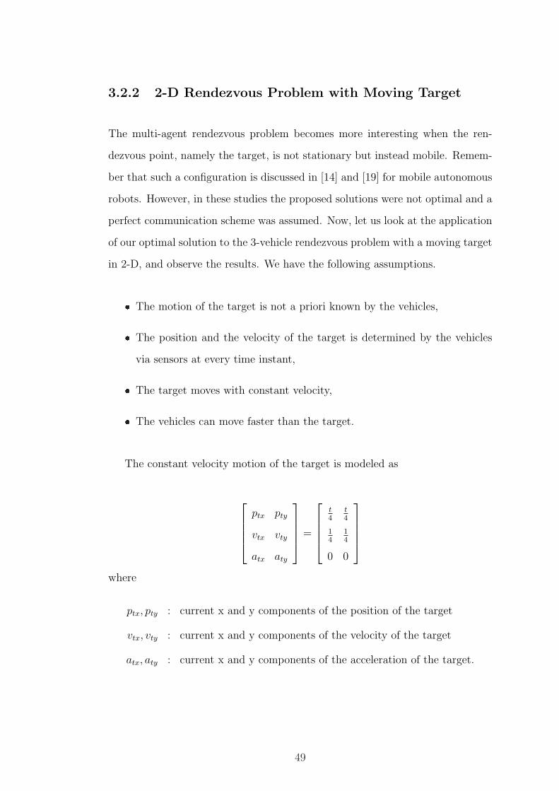
3.2.2 2-D Rendezvous Problem with Moving Target

The multi-agent rendezvous problem becomes more interesting when the ren-

dezvous point, namely the target, is not stationary but instead mobile. Remem-

ber that such a configuration is discussed in [14] and [19] for mobile autonomous

robots. However, in these studies the proposed solutions were not optimal and a

perfect communication scheme was assumed. Now, let us look at the application

of our optimal solution to the 3-vehicle rendezvous problem with a moving target

in 2-D, and observe the results. We have the following assumptions.

� The motion of the target is not a priori known by the vehicles,

� The position and the velocity of the target is determined by the vehicles

via sensors at every time instant,

� The target moves with constant velocity,

� The vehicles can move faster than the target.

The constant velocity motion of the target is modeled as

ptx pty

vtx vty

atx aty

=

t4

t4

14

14

0 0

where

ptx, pty : current x and y components of the position of the target

vtx, vty : current x and y components of the velocity of the target

atx, aty : current x and y components of the acceleration of the target.

49

The problem configuration is same as in 3.6 except the initial and final states.

Also, wi(t) has an effect of ±5% random changes in x and y components of u∗i (t).

The initial states are given as

x1(t0) =

10 5

0 0

0 0

, x2(t0) =

0 15

0 0

0 0

, x3(t0) =

20 0

0 0

0 0

. (3.8)

Since the target moves with constant velocity, the final states can be defined

as

xi(tf ) =

pix(tf ) piy(tf )

vix(tf ) viy(tf )

aix(tf ) aiy(tf )

=

ptx pty

vtx vty

0 0

where

pix(tf ), piy(tf ) : x and y components of the position of vehicle i at tf

vix(tf ), viy(tf ) : x and y components of the velocity of vehicle i at tf

aix(tf ), aiy(tf ) : x and y components of the acceleration of vehicle i at tf

In addition, it is assumed that there is no time delay in the communication.

The results are shown in Figures 3.21 and 3.22

50

−5 0 5 10 15 20−2

0

2

4

6

8

10

12

14

16

x

yPosition

1Position

2Position

3Target

Figure 3.21: Position trajectories for rendezvous in 2-D with moving target

0 2 4 6 8 10 120

0.5

1

1.5

2

2.5

3

3.5

4

4.5

time

velo

citie

s

Velocity1

Velocity2

Velocity3

Target

Figure 3.22: Velocities vs. time for rendezvous in 2-D with moving target

51

As seen in Figures 3.21 and 3.22 the vehicles catch the moving target suc-

cessfully. Now, let us go one step further and consider the time delays in the

communication.

3.2.3 2-D Rendezvous Problem with Moving Target in

the Presence of Communication Problems

As seen in Figures 3.21 and 3.22, it can be concluded that the solution works for

the moving target problem. On the other hand, the solution should be discussed

in the presence of time delays or lost information signals which are very natural

events to be faced with. Next, the result of the application to the problem is

presented with and without considering the uncertainties which were involved in

the model as wi(t)s.

The problem configuration is given as below without including wi(t)s in the

model.

xi = Aixi(t) + Biui(t),

t0 = 0, tf = 10,

x1(t0) =

10 5

0 0

0 0

, x2(t0) =

0 15

0 0

0 0

, x3(t0) =

20 0

0 0

0 0

(3.9)

where Ai and Bi are as in (3.6) and the motion of the target is modeled same as

before. Due to time delay, final times of each vehicle are calculated as explained

in (3.5). hij(k) is modeled as in in (3.4) and hmax is chosen as 0.5 sec.

As seen in Figures 3.23 and 3.24, which are the simulation results without the

effect of wi(t)s, the vehicles catch the moving target and the mission is completed

successfully.

52

However, if we look at Figure 3.25 we can see that the final times are not

equalized successfully. Consequently, the final states of the vehicles are not com-

pletely same as their target. Evidently, this is due to the communication delays

between the vehicles since these delays prevent the vehicles to accurately deter-

mine the actual rendezvous time of the team. Nonetheless, the result is quite

satisfactory.

−5 0 5 10 15 20−2

0

2

4

6

8

10

12

14

16

x

y

Position1

Position2

Position3

Target

Figure 3.23: Position trajectories for rendezvous in 2-D with moving target

53

0 2 4 6 8 10 120

0.5

1

1.5

2

2.5

3

3.5

time

velo

citie

sVelocity

1Velocity

2Velocity

3

Target

Figure 3.24: Velocities vs. time for rendezvous in 2-D with moving target

0 2 4 6 8 10 1210

10.5

11

11.5

12

12.5

13

time

final

tim

e

Final time1

Final time2

Final time3

Figure 3.25: Change in tfi s at communication instants for rendezvous in 2-D with

moving target

54

Now, let us look at the solution if the uncertainties are taken into account

by including wi(t) in the model as a disturbance in the control input. Note

that, missed or late information signals (i.e. the unavailable information) were

also taken into account (as in the previous example) while obtaining the following

solution by utilizing time delays in the communication between the vehicles. The

problem configuration is given as

xi = Aixi(t) + Bi

(([

1 1]

+ wi(t)) · ui(t))

,

t0 = 0, tf = 10,

x1(t0) =

10 5

0 0

0 0

, x2(t0) =

0 15

0 0

0 0

, x3(t0) =

20 0

0 0

0 0

(3.10)

The motion of the target is modeled as

ptx pty

vtx vty

atx aty

=

t2

t2

12

12

0 0

and wi(t) has an effect of ±5% random changes in x and y components of u∗i (t).

The time delays are modeled as before.

Results of the solution are depicted in Figures 3.26-3.28. Looking at Fig-

ure 3.28, we observe that the time delays in the communication cause the vehicles

to determine the rendezvous time differently during the mission, however thanks

to successful information exchange towards the end of the travel, the final ren-

dezvous times are very close. Consequently, we can see that the vehicles achieve

a successful rendezvous as plotted in Figure 3.26. However, the differences in

the rendezvous times caused by the time delays in the communication, result in

deviations from the aimed velocity value of the moving target at the instant of

rendezvous as seen in Figure 3.27.

55

−5 0 5 10 15 20−2

0

2

4

6

8

10

12

14

16

x

y

Position1

Position2

Position3

Target

Figure 3.26: Position trajectories for rendezvous in 2-D with moving target in-

cluding communication problems

0 1 2 3 4 5 6 7 80

1

2

3

4

5

6

time

velo

citie

s

Velocity1

Velocity2

Velocity3

Target

Figure 3.27: Velocities vs. time for rendezvous in 2-D with moving target in-

cluding communication problems

56

0 1 2 3 4 5 6 7 87.5

8

8.5

9

9.5

10

10.5

11

11.5

time

final

tim

e

Final time1

Final time2

Final time3

Figure 3.28: Change in tfi s at communication instants for rendezvous in 2-D with

moving target including communication problems

3.3 Effects of Increasing Disturbance and Time

Delay on the Solution

In this part, we present the solution results for increasing disturbance wi(t) and

time delays hij(k). Various simulations are shown for each case and the results

are discussed. The problem configuration is chosen as in (3.10) and the constant

velocity motion of the target is modeled as

ptx pty

vtx vty

atx aty

=

t4

t4

14

14

0 0

.

57

3.3.1 Increasing Disturbance

In order to observe the effect of disturbance clearly, it is assumed that there

is no time delay in the communication between the vehicles. The disturbance

wi(t) is chosen to be in the form of ± 0, 2, 2.5, 3.33, 5 and 10 % random

changes in the optimal control input u∗i (t). Results are shown in Figures 3.29-

3.31. The observations for increasing disturbance (i.e. the uncertainties) can be

summarized as below.

� Since the disturbances model the uncertainties and they are random, the

rendezvous time and the magnitudes of the disturbances are not related

directly.

� The vehicles catch the moving target successfully in all of the cases, be-

cause the rendezvous time is common for the vehicles thanks to the perfect

communication.

� In general, the magnitudes of the control inputs (except the maximum

values appearing due to the updates in the final time at close instants to

the rendezvous) get larger as the effects of disturbances increase.

58

−5 0 5 10 15 20−2

0

2

4

6

8

10

12

14

16

x

yPosition

1Position

2Position

3Target

(a) ± 0 % random changes in u∗i (t)

−5 0 5 10 15 20−2

0

2

4

6

8

10

12

14

16

x

y

Position1

Position2

Position3

Target

(b) ± 2 % random changes in u∗i (t)

−5 0 5 10 15 20−2

0

2

4

6

8

10

12

14

16

x

y

Position1

Position2

Position3

Target

(c) ± 2.5 % random changes in u∗i (t)

−5 0 5 10 15 20−2

0

2

4

6

8

10

12

14

16

x

y

Position1

Position2

Position3

Target

(d) ± 3.33 % random changes in u∗i (t)

−5 0 5 10 15 20−2

0

2

4

6

8

10

12

14

16

x

y

Position1

Position2

Position3

Target

(e) ± 5 % random changes in u∗i (t)

−5 0 5 10 15 20−2

0

2

4

6

8

10

12

14

16

x

y

Position1

Position2

Position3

Target

(f) ± 10 % random changes in u∗i (t)

Figure 3.29: Position trajectories for increasing disturbances

59

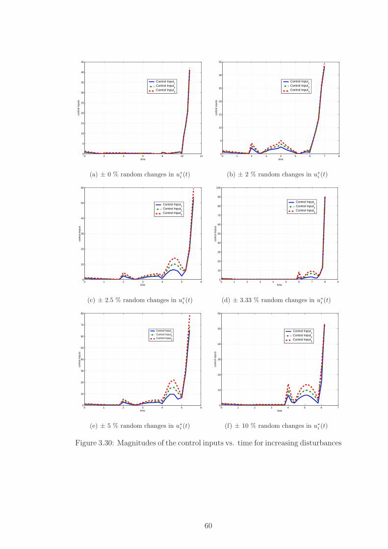
0 2 4 6 8 10 120

5

10

15

20

25

30

35

40

45

time

cont

rol i

nput

sControl Input

1Control Input

2Control Input

3

(a) ± 0 % random changes in u∗i (t)

0 1 2 3 4 5 6 7 80

5

10

15

20

25

30

35

time

cont

rol i

nput

s

Control Input1

Control Input2

Control Input3

(b) ± 2 % random changes in u∗i (t)

0 1 2 3 4 5 60

10

20

30

40

50

60

time

cont

rol i

nput

s

Control Input1

Control Input2

Control Input3

(c) ± 2.5 % random changes in u∗i (t)

0 1 2 3 4 5 6 7 8 90

10

20

30

40

50

60

70

80

90

100

time

cont

rol i

nput

s

Control Input1

Control Input2

Control Input3

(d) ± 3.33 % random changes in u∗i (t)

0 1 2 3 4 5 60

10

20

30

40

50

60

70

80

time

cont

rol i

nput

s

Control Input1

Control Input2

Control Input3

(e) ± 5 % random changes in u∗i (t)

0 1 2 3 4 5 6 70

10

20

30

40

50

60

time

cont

rol i

nput

s

Control Input1

Control Input2

Control Input3

(f) ± 10 % random changes in u∗i (t)

Figure 3.30: Magnitudes of the control inputs vs. time for increasing disturbances

60

0 2 4 6 8 10 1210

11

12

13

14

15

16

17

time

final

tim

e

Final Time

(a) ± 0 % random changes in u∗i (t)

0 1 2 3 4 5 6 7 86.5

7

7.5

8

8.5

9

9.5

10

time

final

tim

e

Final time

(b) ± 2 % random changes in u∗i (t)

0 1 2 3 4 5 65.5

6

6.5

7

7.5

8

8.5

9

9.5

10

time

final

tim

e

Final time

(c) ± 2.5 % random changes in u∗i (t)

0 1 2 3 4 5 6 7 8 98

9

10

11

12

13

14

15

16

17

time

final

tim

e

Final time

(d) ± 3.33 % random changes in u∗i (t)

0 1 2 3 4 5 65.5

6

6.5

7

7.5

8

8.5

9

9.5

10

time

final

tim

e

Final time

(e) ± 5 % random changes in u∗i (t)

0 1 2 3 4 5 6 76

7

8

9

10

11

12

13

time

final

tim

e

Final Time

(f) ± 10 % random changes in u∗i (t)

Figure 3.31: Final times vs. time for increasing disturbances

61

3.3.2 Increasing Time Delay

In order to observe the effect of increasing time delay in the communication,

solutions corresponding to various time delays are obtained. The waiting time

hmax is 0.5 sec as before. The delay model is similar to (3.4)

hik ∼ |N(hmean, 0.05)| (3.11)

i.e. we have normally distributed positive time delay values with mean hmean and

variance 0.05. Thus, we can observe the effect of time delay in the communication

by increasing its mean while keeping the variance small. We obtain the solutions

for different values of hmean as 0.1, 0.3, 0.4, 0.45, 0.49, 0.5, 0.8 and 1.3 sec. It

is assumed that there is no disturbance (i.e. wi(t) = 0). Results are shown

in Figures 3.32-3.34. The observations for increasing waiting time hmax can be

summarized as below.

� Increasing the mean of the random time delay results in deviations in ren-

dezvous time information. If time delays exceed the maximum waiting time

at a communication instant, the vehicles cannot have a common rendezvous

time until the next successful communication.

� If most of the time delays are greater than the waiting time during the

travel, the success of the mission depends on reliable information exchanges

as the rendezvous time approaches. If successful communication is not

achieved towards the end of the travel, the rendezvous does not occur.

� As expected, the rendezvous is not achieved if time delays in the communi-

cation are greater than the maximum waiting time. Therefore, the waiting

time should be chosen carefully according to the expected time delays in

the communication.

62

−5 0 5 10 15 20−2

0

2

4

6

8

10

12

14

16

x

y

Position1

Position2

Position3

Target

(a) hmean = 0.1 sec

−5 0 5 10 15 20−2

0

2

4

6

8

10

12

14

16

x

y

Position1

Position2

Position3

Target

(b) hmean = 0.3 sec

−5 0 5 10 15 20−2

0

2

4

6

8

10

12

14

16

x

y

Position1

Position2

Position3

Target

(c) hmean = 0.4 sec

−5 0 5 10 15 20−2

0

2

4

6

8

10

12

14

16

x

y

Position1

Position2

Position3

Target

(d) hmean = 0.45 sec

−5 0 5 10 15 20−2

0

2

4

6

8

10

12

14

16

x

y

Position1

Position2

Position3

Target

(e) hmean = 0.49

−5 0 5 10 15 20−2

0

2

4

6

8

10

12

14

16

x

y

Position1

Position2

Position3

Target

(f) hmean = 0.5 sec

−5 0 5 10 15 20−2

0

2

4

6

8

10

12

14

16

x

y

Position1

Position2

Position3

Target

(g) hmean = 0.8 sec

−5 0 5 10 15 20−2

0

2

4

6

8

10

12

14

16

x

y

Position1

Position2

Position3

Target

(h) hmean = 1.1 sec

Figure 3.32: Position trajectories for increasing time delay in the communication

63

0 1 2 3 4 5 6 70

10

20

30

40

50

60

70

80

time

cont

rol i

nput

s

Control Input1

Control Input2

Control Input3

(a) hmean = 0.1 sec

0 1 2 3 4 5 6 7 80

5

10

15

20

25

30

35

40

45

time

cont

rol i

nput

s

Control Input1

Control Input2

Control Input3

(b) hmean = 0.3 sec

0 2 4 6 8 10 120

5

10

15

20

25

30

35

40

45

time

cont

rol i

nput

s

Control Input1

Control Input2

Control Input3

(c) hmean = 0.4 sec

0 2 4 6 8 10 120

20

40

60

80

100

120

140

160

180

time

cont

rol i

nput

s

Control Input1

Control Input2

Control Input3

(d) hmean = 0.45 sec

0 1 2 3 4 5 6 70

100

200

300

400

500

600

time

cont

rol i

nput

s

Control Input1

Control Input2

Control Input3

(e) hmean = 0.49

0 1 2 3 4 5 6 70

10

20

30

40

50

60

time

cont

rol i

nput

s

Control Input1

Control Input2

Control Input3

(f) hmean = 0.5 sec

0 1 2 3 4 5 6 7 80

10

20

30

40

50

60

time

cont

rol i

nput

s

Control Input1

Control Input2

Control Input3

(g) hmean = 0.8 sec

0 1 2 3 4 5 6 7 80

20

40

60

80

100

120

140

160

180

time

cont

rol i

nput

s

Control Input1

Control Input2

Control Input3

(h) hmean = 1.1 sec

Figure 3.33: Magnitudes of the control inputs vs. time for increasing time delay

in the communication

64

0 1 2 3 4 5 6 76

6.5

7

7.5

8

8.5

9

9.5

10

time

final

tim

e

Final time1

Final time2

Final time3

(a) hmean = 0.1 sec

0 1 2 3 4 5 6 7 86

6.5

7

7.5

8

8.5

9

9.5

10

time

final

tim

e

Final time1

Final time2

Final time3

(b) hmean = 0.3 sec

0 2 4 6 8 10 1210

11

12

13

14

15

16

17

18

19

time

final

tim

e

Final time1

Final time2

Final time3

(c) hmean = 0.4 sec

0 2 4 6 8 10 1210

10.5

11

11.5

12

12.5

13

13.5

time

final

tim

e

Final time1

Final time2

Final time3

(d) hmean = 0.45 sec

0 1 2 3 4 5 6 76

6.5

7

7.5

8

8.5

9

9.5

10

time

final

tim

e

Final time1

Final time2

Final time3

(e) hmean = 0.49

0 1 2 3 4 5 6 76

6.5

7

7.5

8

8.5

9

9.5

10

time

final

tim

e

Final time1

Final time2

Final time3

(f) hmean = 0.5 sec

0 1 2 3 4 5 6 7 87

7.5

8

8.5

9

9.5

10

time

final

tim

e

Final time1

Final time2

Final time3

(g) hmean = 0.8 sec

0 1 2 3 4 5 6 7 87

7.5

8

8.5

9

9.5

10

time

final

tim

e

Final time1

Final time2

Final time3

(h) hmean = 1.1 sec

Figure 3.34: Final times vs. time for increasing time delay in the communication

65

Chapter 4

CONCLUSIONS

In this study, the multi-agent rendezvous problem is discussed. The problem

consists of N > 1 mobile agents, which are trying to reach a destination (i.e.

the rendezvous point) simultaneously. It is assumed that the initial and the final

states of the agents as well as a target value for the rendezvous time are specified.

Even it seems reasonable to expect the agents to reach the destination at the pre-

specified rendezvous time, desired rendezvous may not be possible due to some

unforeseen events like obstacles on the road, internal problems of the agents or

any other disturbance. Therefore, a communication scheme is utilized between

the agents in order to enable an exchange of information about the estimated

times of arrivals of the agents with regular time intervals. The reason for having

the information exchanges at discrete time instants is simply the cost of reliable

continuous communication.

In order to solve this multi-agent rendezvous problem, an appropriate cost

function is defined and solved for the minimizing control input. The solution for

the problem is based on minimum energy control which is a very useful extension

of calculus of variations, and the results are quite satisfactory that the optimal

66

solutions obtained at each communication instant successively realize a simulta-

neous rendezvous despite unexpected disturbances. Initially, the solution is given

in 1-D and does not take into account the problems in information exchange, like

delayed or lost signals. Therefore, an algorithm is proposed for handling delayed

or lost information, and the solution is extended to 2-D including moving target

point case. In this case the agents try to catch a mobile target simultaneously.

Such a problem appears in several applications, e.g. optimal motion or trajectory

planning for UAVs, robot teams and vehicle convoys. The effect of increasing

disturbance on the control input and time delays in the communication are also

discussed.

In addition, it is possible to make some improvements in order to have a

more comprehensive solution. For instance, it may be a good complementary

study to develop an estimator for the signals carrying information about the

rendezvous times of the agents since these signals may be delayed and noisy

or completely lost, rather than using the proposed algorithm in the solution

for handling the same problem. Also, another complementary study may be

adapting collision/obstacle avoidance to the solution which is very important for

vehicles or robots working autonomously.

67

APPENDIX A

Matlab code for the solution of

rendezvous in 1-D

1 clear;

2 clc;

3

4 A = [0 1 0;0 0 1;0 0 0];

5 B = [0;0;1];

6 x1 0 = [10;0;0];

7 x2 0 = [15;0;0];

8 x3 0 = [20;0;0];

9 x0 1 = x1 0;

10 x0 2 = x2 0;

11 x0 3 = x3 0;

12 xf = [0;0;0];ts = 0;

13 tf = 20;

14 tb= ts;

15 te= tf;

16 inc = (tf−ts)/50;17 hmax = (tf−ts)/20;18 hmean = 0;

19 hst = hmax*0.90;

20 syms t p;

21 x 1 = [];

22 u 1 = [];

23 x 2 = [];

24 u 2 = [];

25 x 3 = [];

26 u 3 = [];

27 tem = [];

28 tmr = [];

29 tm = tb;

30 tm c = tm;

31 t t1 = [];

32 t t2 = [];

33 t t3 = [];

34 te t = [te;te;te];

35 te calc = [te;te;te];

36 te r = [te];

37 h =[0;0;0];

38

39 while tm < te

40 % Expected arrival times are determined here

41 if length(tmr) > 0 && mod(length(tmr),10) == 0

42 [i1 i2] = size(te calc);

43 in = length(tmr);

44 c1 = ([(tmr(in−4)ˆ4) (tmr(in−4)ˆ3) (tmr(in−4)ˆ2) ...

45 tmr(in−4) 1; (tmr(in−3)ˆ4) (tmr(in−3)ˆ3) ...

46 (tmr(in−3)ˆ2) tmr(in−3) 1;(tmr(in−2)ˆ4) ...

47 (tmr(in−2)ˆ3) (tmr(in−2)ˆ2) tmr(in−2) 1;...

48 (tmr(in−1)ˆ4) (tmr(in−1)ˆ3) (tmr(in−1)ˆ2)...49 tmr(in−1) 1;(tmr(in)ˆ4) (tmr(in)ˆ3) (tmr(in)ˆ2)...

50 tmr(in) 1] \ ...

51 [x 1(2,in−4);x 1(2,in−3);x 1(2,in−2);...52 x 1(2,in−1);x 1(2,in)]);

53

54 t t 1 = roots([(c1(1)/5) (c1(2)/4) (c1(3)/3)...

55 (c1(4)/2) c1(5)−((c1(1)/5)*(tmr(in)ˆ5)+(c1(2)/4)*...56 (tmr(in)ˆ4)+(c1(3)/3)*(tmr(in)ˆ3)+(c1(4)/2)*...

57 (tmr(in)ˆ2)+c1(5)*tmr(in)+(xf(1)−x 1(1,in)))]);

58 t t1 = [t t1 t t 1];

59 temp1 = [];

60 for i=1:1:5

61 if abs(imag(t t 1(i)))≤1e−362 t t 1(i) = real(t t 1(i));

63 end

64 end

68

65 for i=1:1:5

66 temp1(i) = isreal(t t 1(i)) && 0<t t 1(i);

67 end

68 te 1 = max(temp1'.*t t 1);

69

70 c2 = ([(tmr(in−4)ˆ4) (tmr(in−4)ˆ3)...71 (tmr(in−4)ˆ2) tmr(in−4) 1; (tmr(in−3)ˆ4)...72 (tmr(in−3)ˆ3) (tmr(in−3)ˆ2) tmr(in−3) 1;...

73 (tmr(in−2)ˆ4) (tmr(in−2)ˆ3) (tmr(in−2)ˆ2)...74 tmr(in−2) 1; (tmr(in−1)ˆ4) (tmr(in−1)ˆ3)...75 (tmr(in−1)ˆ2) tmr(in−1) 1; (tmr(in)ˆ4)...

76 (tmr(in)ˆ3) (tmr(in)ˆ2) tmr(in) 1] \...77 [x 2(2,in−4);x 2(2,in−3);x 2(2,in−2);...78 x 2(2,in−1);x 2(2,in)]);

79

80 t t 2 = roots([(c2(1)/5) (c2(2)/4)...

81 (c2(3)/3) (c2(4)/2) c2(5)−((c2(1)/5)*...82 (tmr(in)ˆ5)+(c2(2)/4)*(tmr(in)ˆ4)+...

83 (c2(3)/3)*(tmr(in)ˆ3)+(c2(4)/2)*...

84 (tmr(in)ˆ2)+c2(5)*tmr(in)+(xf(1)−...85 x 2(1,in)))]);

86

87 t t2 = [t t2 t t 2];

88 temp2 = [];

89 for i=1:1:5

90 if abs(imag(t t 2(i)))≤1e−391 t t 2(i) = real(t t 2(i));

92 end

93 end

94 for i=1:1:5

95 temp2(i) = isreal(t t 2(i)) && 0<t t 2(i);

96 end

97 te 2 = max(temp2'.*t t 2);

98

99 c3 = ([(tmr(in−4)ˆ4) (tmr(in−4)ˆ3)...100 (tmr(in−4)ˆ2) tmr(in−4) 1;(tmr(in−3)ˆ4)...101 (tmr(in−3)ˆ3) (tmr(in−3)ˆ2) tmr(in−3) 1;...

102 (tmr(in−2)ˆ4) (tmr(in−2)ˆ3) (tmr(in−2)ˆ2)...103 tmr(in−2) 1;(tmr(in−1)ˆ4) (tmr(in−1)ˆ3)...104 (tmr(in−1)ˆ2) tmr(in−1) 1;(tmr(in)ˆ4)...

105 (tmr(in)ˆ3) (tmr(in)ˆ2) tmr(in) 1] \...106 [x 3(2,in−4);x 3(2,in−3);x 3(2,in−2);...107 x 3(2,in−1);x 3(2,in)]);

108

109 t t 3 = roots([(c3(1)/5) (c3(2)/4)...

110 (c3(3)/3) (c3(4)/2) c3(5)−((c3(1)/5)*...111 (tmr(in)ˆ5)+(c3(2)/4)*(tmr(in)ˆ4)+...

112 (c3(3)/3)*(tmr(in)ˆ3)+(c3(4)/2)*...

113 (tmr(in)ˆ2)+c3(5)*tmr(in)+(xf(1)−...114 x 3(1,in)))]);

115

116 t t3 = [t t3 t t 3];

117 temp3 = [];

118 for i=1:1:5

119 if abs(imag(t t 3(i)))≤1e−3120 t t 3(i) = real(t t 3(i));

121 end

122 end

123 for i=1:1:5

124 temp3(i) = isreal(t t 3(i)) && 0<t t 3(i);

125 end

126 te 3= max(temp3'.*t t 3);

127

128 te calc = [te calc [te 1;te 2;te 3]];

129 te r =[te r min([te 1;te 2;te 3])];

130 tm c = tm;

131 % Time delay matrix is formed here

132 h1 = (hmean) + hst*abs(randn);

133 h2 = (hmean) + hst*abs(randn);

134 h3 = (hmean) + hst*abs(randn);

135 h = [h [h1;h2;h3]];

136 te t = [te t [te;te;te]];

137 end

138

139 %−−−−−−−−−−−−−−−−−−−−−−−−−−−−−−−−−−−−−−−−−−−−−−−−−−−−−−−−−140 % Rendezvous time information is updated below

141 [in1 in2] = size(h);

142 for i=1:3

143 if (h(i,in2) ≤ hmax) && ((tm c + h(i,in2))≤ tm)

144 te t(i,in2) = te calc (i,in2);

145 end

146 end

147 te = min(te t(:,(in2)));

148

149 %−−−−−−−−−−−−−−−−−−−−−−−−−−−−−−−−−−−−−−−−−−−−−−−−−−−−−−−−−−−−−150 % Terms related with the Controllability Matrix W c are below

151 Wc = int(expm(A*(tb−t))*B*B'*expm(A'*(tb−t)),t,tb,te);152 eat = expm(A'*(tb−t));153 ea = expm(A*(tb−te));154

155 %−−−−−−−−−−−−−−−−−−−−−−−−−−−−−−−−−−−−−−−−−−−−−−−−−−−−−−−−−−−−−−−156 % Here, control inputs are calculated and disturbances are added

157 up 1 = − B'*eat*inv(Wc)*(x0 1−ea*xf);158 up 1 = up 1;

159 up 1 = up 1 + (up 1/50)*((rand>0.9)*randn);

160 up 2 = − B'*eat*inv(Wc)*(x0 2−ea*xf);161 up 2 = up 2;

162 up 2 = up 2 + (up 2/50)*((rand>0.9)*randn);

163 up 3 = − B'*eat*inv(Wc)*(x0 3−ea*xf);164 up 3 = up 3;

165 up 3 = up 3 + (up 3/50)*((rand>0.9)*randn);

166

167

168 %−−−−−−−−−−−−−−−−−−−−−−−−−−−−−−−−−−−−−−−−−−−−−−169 % Solutions are obtained below

170 d 1 = int(expm(A*(p−t))*B*up 1,t,tb,p);

171 xp1 1 = subs(d 1,p,tm);

172 up1 1 = subs(− B'*eat*inv(Wc)*(x0 1−ea*xf),t,tm);173 xp 1 = ((expm(A*(tm−tb))*x0 1) + (xp1 1 ));

174 d 2 = int(expm(A*(p−t))*B*up 2,t,tb,p);

175 xp2 1 = subs(d 2,p,tm);

176 up2 1 = subs(− B'*eat*inv(Wc)*(x0 2−ea*xf),t,tm);177 xp 2 = ((expm(A*(tm−tb))*x0 2) + (xp2 1 ));

178 d 3 = int(expm(A*(p−t))*B*up 3,t,tb,p);

179 xp3 1 = subs(d 3,p,tm);

180 up3 1 = subs(− B'*eat*inv(Wc)*(x0 3−ea*xf),t,tm);181 xp 3 = ((expm(A*(tm−tb))*x0 3) + (xp3 1 ));

182

183

184

69

185 %−−−−−−−−−−−−−−−−−−−−−−−−−−−−−−−−−−−−−−−−−−−−−186 % Here, solutions are added into corresponding

187 % matrices

188 x 1 = [x 1 xp 1];

189 u 1 = [u 1 up1 1];

190 x 2 = [x 2 xp 2];

191 u 2 = [u 2 up2 1];

192 x 3 = [x 3 xp 3];

193 u 3 = [u 3 up3 1];

194

195 %−−−−−−−−−−−−−−−−−−−−−−−−−−−−−−−−−−−−−−−−−−−−−−−−−−−−−−−−−196 % Required simulation updates are made below

197 tem = [tem te];

198 tmr = [tmr tm];

199 tb = tm;

200 tm = tm + inc;

201 x0 1 = xp 1;

202 x0 2 = xp 2;

203 x0 3 = xp 3;

204 end

70

APPENDIX B

Matlab code for the solution of

rendezvous in 2-D

1 clear;

2 clc;

3

4 A = [0 1 0;0 0 1;0 0 0];

5 B = [0;0;1];

6 x1 0 = [10 5;0 0;0 0];

7 x2 0 = [0 15;0 0;0 0];

8 x3 0 = [20 0;0 0;0 0];

9 x0 1 = x1 0;

10 x0 2 = x2 0;

11 x0 3 = x3 0;

12 xf = [0 0;0 0;0 0];

13 xf 1 = [];

14 ts = 0;

15 tf = 10;

16 tb= ts;

17 te= tf;

18 inc = (tf−ts)/50;19 hmax = 0.5;

20 hmean = 0;

21 hst = hmax*0.90;

22 syms t p;

23 x 1 = [];

24 u 1 = [];

25 x 2 = [];

26 u 2 = [];

27 x 3 = [];

28 u 3 = [];

29 tem = [];

30 tmr = [];

31 tm = tb;

32 tm c = tm;

33 t t1 = [];

34 t t2 = [];

35 t t3 = [];

36 te t = [];

37 te calc = [te;te;te];

38 te r = [te];

39 te h = ones(3,1)*te;

40 te rec = [];

41 h = zeros(3);

42 st 1 = [];

43 st 2 = [];

44 st 3 = [];

45

46 while (tm) < min(te)

47 % Expected arrival times are determined here

48 if length(tmr) > 1 && mod(length(tmr),10) == 0

49 in = length(tmr);

50 c1 = ([(tmr(in−4)ˆ4) (tmr(in−4)ˆ3) (tmr(in−4)ˆ2)...51 tmr(in−4) 1; (tmr(in−3)ˆ4) (tmr(in−3)ˆ3)...52 (tmr(in−3)ˆ2) tmr(in−3) 1; (tmr(in−2)ˆ4)...53 (tmr(in−2)ˆ3) (tmr(in−2)ˆ2) tmr(in−2) 1;...

54 (tmr(in−1)ˆ4) (tmr(in−1)ˆ3) (tmr(in−1)ˆ2)...55 tmr(in−1) 1; (tmr(in)ˆ4) (tmr(in)ˆ3) (tmr(in)ˆ2)...

56 tmr(in) 1] \...57 [x 1(2,(2*in−9));x 1(2,(2*in−7));x 1(2,(2*in−5));...58 x 1(2,(2*in−3));x 1(2,(2*in−1))]);59

60 t t 1 = roots([(c1(1)/5) (c1(2)/4) (c1(3)/3)...

61 (c1(4)/2) c1(5)−((c1(1)/5)*(tmr(in)ˆ5)+(c1(2)/4)...62 *(tmr(in)ˆ4)+(c1(3)/3)*(tmr(in)ˆ3)+(c1(4)/2)*...

63 (tmr(in)ˆ2)+c1(5)*tmr(in) + (xf(1,1)−...64 x 1(1,(2*in−1))))]);

71

65

66 t t1 = [t t1 t t 1];

67 temp1 = [];

68 for i=1:1:5

69 if abs(imag(t t 1(i)))≤1e−370 t t 1(i) = real(t t 1(i));

71 end

72 end

73 for i=1:1:5

74 temp1(i) = isreal(t t 1(i)) && 0<t t 1(i);

75 end

76 te 1 x = max(temp1'.*t t 1);

77

78 in = length(tmr);

79 c1 = ([(tmr(in−4)ˆ4) (tmr(in−4)ˆ3...80 (tmr(in−4)ˆ2) tmr(in−4) 1;(tmr(in−3)ˆ4)...81 (tmr(in−3)ˆ3) (tmr(in−3)ˆ2) tmr(in−3) 1;...

82 (tmr(in−2)ˆ4) (tmr(in−2)ˆ3) (tmr(in−2)ˆ2)...83 tmr(in−2) 1;(tmr(in−1)ˆ4) (tmr(in−1)ˆ3)...84 (tmr(in−1)ˆ2) tmr(in−1) 1;(tmr(in)ˆ4)...

85 (tmr(in)ˆ3) (tmr(in)ˆ2) tmr(in) 1] \...86 [x 1(2,(2*in−8));x 1(2,(2*in−6));...87 x 1(2,(2*in−4)); x 1(2,(2*in−2));...88 x 1(2,(2*in))]);

89

90 t t 1 = roots([(c1(1)/5) (c1(2)/4)...

91 (c1(3)/3) (c1(4)/2) c1(5)−((c1(1)/5)*92 (tmr(in)ˆ5)+(c1(2)/4)*(tmr(in)ˆ4)+...

93 (c1(3)/3)*(tmr(in)ˆ3)+(c1(4)/2)*...

94 (tmr(in)ˆ2)+c1(5)*tmr(in) + (xf(1,1)−...95 x 1(1,(2*in))))]);

96

97 t t1 = [t t1 t t 1];

98 temp1 = [];

99 for i=1:1:5

100 if abs(imag(t t 1(i)))≤1e−3101 t t 1(i) = real(t t 1(i));

102 end

103 end

104 for i=1:1:5

105 temp1(i) = isreal(t t 1(i)) && 0<t t 1(i);

106 end

107 te 1 y = max(temp1'.*t t 1);

108 te 1 = min(te 1 x,te 1 y);

109

110 c2 = ([(tmr(in−4)ˆ4) (tmr(in−4)ˆ3)...111 (tmr(in−4)ˆ2) tmr(in−4) 1;(tmr(in−3)ˆ4)...112 (tmr(in−3)ˆ3) (tmr(in−3)ˆ2) tmr(in−3) 1;...

113 (tmr(in−2)ˆ4) (tmr(in−2)ˆ3) (tmr(in−2)ˆ2)...114 tmr(in−2) 1; (tmr(in−1)ˆ4) (tmr(in−1)ˆ3)...115 (tmr(in−1)ˆ2) tmr(in−1) 1;(tmr(in)ˆ4)...

116 (tmr(in)ˆ3) (tmr(in)ˆ2) tmr(in) 1] \...117 [x 2(2,(2*in−9));x 2(2,(2*in−7));...118 x 2(2,(2*in−5)); x 2(2,(2*in−3));...119 x 2(2,(2*in−1))]);120

121 t t 2 = roots([(c2(1)/5) (c2(2)/4)...

122 (c2(3)/3) (c2(4)/2) c2(5)−((c2(1)/5)*...123 (tmr(in)ˆ5)+(c2(2)/4)*(tmr(in)ˆ4)+...

124 (c2(3)/3)*(tmr(in)ˆ3)+(c2(4)/2)*...

125 (tmr(in)ˆ2)+c2(5)*tmr(in) + (xf(1,1)−...126 x 2(1,(2*in−1))))]);127

128 t t2 = [t t2 t t 2];

129 temp2 = [];

130 for i=1:1:5

131 if abs(imag(t t 2(i)))≤1e−3132 t t 2(i) = real(t t 2(i));

133 end

134 end

135 for i=1:1:5

136 temp2(i) = isreal(t t 2(i)) && 0<t t 2(i);

137 end

138 te 2 x = max(temp2'.*t t 2);

139

140 c2 = ([(tmr(in−4)ˆ4) (tmr(in−4)ˆ3)...141 (tmr(in−4)ˆ2) tmr(in−4) 1; (tmr(in−3)ˆ4)...142 (tmr(in−3)ˆ3) (tmr(in−3)ˆ2) tmr(in−3) 1;...

143 (tmr(in−2)ˆ4) (tmr(in−2)ˆ3) (tmr(in−2)ˆ2)...144 tmr(in−2) 1; (tmr(in−1)ˆ4) (tmr(in−1)ˆ3)...145 (tmr(in−1)ˆ2) tmr(in−1) 1; (tmr(in)ˆ4)...

146 (tmr(in)ˆ3) (tmr(in)ˆ2) tmr(in) 1] \...147 [x 2(2,(2*in−8));x 2(2,(2*in−6));...148 x 2(2,(2*in−4)); x 2(2,(2*in−2));...149 x 2(2,(2*in))]);

150

151 t t 2 = roots([(c2(1)/5) (c2(2)/4)...

152 (c2(3)/3) (c2(4)/2) c2(5)−...153 ((c2(1)/5)*(tmr(in)ˆ5)+(c2(2)/4)*...

154 (tmr(in)ˆ4)+(c2(3)/3)*(tmr(in)ˆ3)+...

155 (c2(4)/2)*(tmr(in)ˆ2)+...

156 c2(5)*tmr(in) + (xf(1,1)−...157 x 2(1,(2*in))))]);

158

159 t t2 = [t t2 t t 2];

160 temp2 = [];

161 for i=1:1:5

162 if abs(imag(t t 2(i)))≤1e−3163 t t 2(i) = real(t t 2(i));

164 end

165 end

166 for i=1:1:5

167 temp2(i) = isreal(t t 2(i)) && 0<t t 2(i);

168 end

169 te 2 y = max(temp2'.*t t 2);

170 te 2 = min(te 2 x,te 2 y);

171

172 c3 = ([(tmr(in−4)ˆ4) (tmr(in−4)ˆ3)...173 (tmr(in−4)ˆ2) tmr(in−4) 1;...

174 (tmr(in−3)ˆ4) (tmr(in−3)ˆ3) (tmr(in−3)ˆ2)...175 tmr(in−3) 1; tmr(in−2)ˆ4) (tmr(in−2)ˆ3)...176 (tmr(in−2)ˆ2) tmr(in−2) 1;(tmr(in−1)ˆ4)...177 (tmr(in−1)ˆ3) (tmr(in−1)ˆ2) tmr(in−1) 1;...

178 (tmr(in)ˆ4) (tmr(in)ˆ3) (tmr(in)ˆ2) tmr(in) 1] \...179 [x 3(2,(2*in−9));x 3(2,(2*in−7));...180 x 3(2,(2*in−5)); x 3(2,(2*in−3));...181 x 3(2,(2*in−1))]);182

183 t t 3 = roots([(c3(1)/5) (c3(2)/4) (c3(3)/3)...

184 (c3(4)/2) c3(5)−((c3(1)/5)*(tmr(in)ˆ5)+...

72

185 (c3(2)/4)*(tmr(in)ˆ4)+(c3(3)/3)*...

186 (tmr(in)ˆ3)+(c3(4)/2)*(tmr(in)ˆ2)+c3(5)*...

187 tmr(in)+(xf(1,1)−x 3(1,(2*in−1))))]);188

189 t t3 = [t t3 t t 3];

190 temp3 = [];

191 for i=1:1:5

192 if abs(imag(t t 3(i)))≤1e−3193 t t 3(i) = real(t t 3(i));

194 end

195 end

196 for i=1:1:5

197 temp3(i) = isreal(t t 3(i)) && 0<t t 3(i);

198 end

199 te 3 x = max(temp3'.*t t 3);

200

201 c3 = ([(tmr(in−4)ˆ4) (tmr(in−4)ˆ3)...202 (tmr(in−4)ˆ2) tmr(in−4) 1; (tmr(in−3)ˆ4)...203 (tmr(in−3)ˆ3) (tmr(in−3)ˆ2) tmr(in−3) 1;...

204 (tmr(in−2)ˆ4) (tmr(in−2)ˆ3) (tmr(in−2)ˆ2)...205 tmr(in−2) 1; (tmr(in−1)ˆ4) (tmr(in−1)ˆ3)...206 (tmr(in−1)ˆ2) tmr(in−1) 1; (tmr(in)ˆ4)...

207 (tmr(in)ˆ3) (tmr(in)ˆ2) tmr(in) 1] \...208 [x 3(2,(2*in−8));x 3(2,(2*in−6));...209 x 3(2,(2*in−4)); x 3(2,(2*in−2));...210 x 3(2,(2*in))]);

211

212 t t 3 = roots([(c3(1)/5) (c3(2)/4)...

213 (c3(3)/3) c3(4)/2) c3(5)−((c3(1)/5)*...214 (tmr(in)ˆ5)+(c3(2)/4)*(tmr(in)ˆ4)+...

215 (c3(3)/3)*(tmr(in)ˆ3)+(c3(4)/2)*...

216 (tmr(in)ˆ2)+c3(5)*tmr(in)+ (xf(1,1)−...217 x 3(1,(2*in))))]);

218

219 t t3 = [t t3 t t 3];

220 temp3 = [];

221 for i=1:1:5

222 if abs(imag(t t 3(i)))≤1e−3223 t t 3(i) = real(t t 3(i));

224 end

225 end

226 for i=1:1:5

227 temp3(i) = isreal(t t 3(i)) && 0<t t 3(i);

228 end

229 te 3 y = max(temp3'.*t t 3);

230 te 3 = min(te 3 x,te 3 y);

231

232 te calc = [te calc [te 1;te 2;te 3]];

233 te r =[te r min([te 1;te 2;te 3])];

234 tm c = tm;

235 % Time delay matrix is formed here

236 h t = hmean + hst*abs(randn(3));

237 h = [h h t];

238 te t = [te t te h];

239 te rec = [te rec te];

240 end

241 %−−−−−−−−−−−−−−−−−−−−−−−−−−−−−−−−−−−−−−−−−−−−−−−−−242 % Rendezvous time information is updated below

243 [in1 in2] = size(h);

244 in21 =in2/3;

245 for i=1:1:3

246 for j=0:1:2

247 if (h(i,in2−j) ≤ hmax) && ((tm c + h(i,in2−j))≤ tm)

248 te h(i,3−j) = te calc (3−j,in21);249 end

250 if (i==(3−j))251 te h(i,3−j) = te calc (3−j,in21);252 end

253 end

254 end

255 te = min(te h');

256 %−−−−−−−−−−−−−−−−−−−−−−−−−−−−−−−−−−−−−−−−−−−−−−−−−−−−−−−−−−−−−257 % Terms related with the Controllability Matrix W c are below

258 Wc1 = int(expm(A*(tb−t))*B*B'*expm(A'*(tb−t)),t,tb,te(1));259 eat1 = expm(A'*(tb−t));260 ea1 = expm(A*(tb−te(1)));261 Wc2 = int(expm(A*(tb−t))*B*B'*expm(A'*(tb−t)),t,tb,te(2));262 eat2 = expm(A'*(tb−t));263 ea2 = expm(A*(tb−te(2)));264 Wc3 = int(expm(A*(tb−t))*B*B'*expm(A'*(tb−t)),t,tb,te(3));265 eat3 = expm(A'*(tb−t));266 ea3 = expm(A*(tb−te(3)));267 %−−−−−−−−−−−−−−−−−−−−−−−−−−−−−−−−−−−−−−−−−−−−−−−−−−−−−−−−−−−−−−−268 % Here, control inputs are calculated and disturbances are added

269 up 1= − B'*eat1*inv(Wc1)*(x0 1−ea1*xf);270 up 1 = up 1;

271 up 1 = up 1 + (up 1/50).*((rand>0.9)*randn(1,2));

272 up 2 = − B'*eat2*inv(Wc2)*(x0 2−ea2*xf);273 up 2 = up 2;

274 up 2 = up 2 + (up 2/50).*((rand>0.9)*randn(1,2));

275 up 3 = − B'*eat3*inv(Wc3)*(x0 3−ea3*xf);276 up 3 = up 3;

277 up 3 = up 3 + (up 3/50).*((rand>0.9)*randn(1,2));

278 %−−−−−−−−−−−−−−−−−−−−−−−−−−−−−−−−−−−−−−−−−−−−−−−−−−−−−−−−−279 % Solutions are obtained below

280 d 1 = int(expm(A*(p−t))*B*up 1,t,tb,p);

281 xp1 1 = subs(d 1,p,tm);

282 up1 1 = subs(− B'*eat1*inv(Wc1)*(x0 1−ea1*xf),t,tm);283 xp 1 = ((expm(A*(tm−tb))*x0 1) + (xp1 1 ));

284 d 2 = int(expm(A*(p−t))*B*up 2,t,tb,p);

285 xp2 1 = subs(d 2,p,tm);

286 up2 1 = subs(− B'*eat2*inv(Wc2)*(x0 2−ea2*xf),t,tm);287 xp 2 = ((expm(A*(tm−tb))*x0 2) + (xp2 1 ));

288 d 3 = int(expm(A*(p−t))*B*up 3,t,tb,p);

289 xp3 1 = subs(d 3,p,tm);

290 up3 1 = subs(− B'*eat3*inv(Wc3)*(x0 3−ea3*xf),t,tm);291 xp 3 = ((expm(A*(tm−tb))*x0 3) + (xp3 1 ));

292 %−−−−−−−−−−−−−−−−−−−−−−−−−−−−−−−−−−−−−−−−−−−−−−−−−−−−−−−−−293 % Here, solutions are added into corresponding matrices

294 x 1 = [x 1 xp 1];

295 u 1 = [u 1 up1 1];

296 x 2 = [x 2 xp 2];

297 u 2 = [u 2 up2 1];

298 x 3 = [x 3 xp 3];

299 u 3 = [u 3 up3 1];

300 %−−−−−−−−−−−−−−−−−−−−−−−−−−−−−−−−−−−−−−−−−−−−−−−−−−−−−−−−−301 % States are collected in single matrices for each vehicle

302 st 1 = [st 1; xp 1(1,1) xp 1(1,2) xp 1(2,1)...

303 xp 1(2,2) xp 1(3,1) xp 1(3,2)...

304 up1 1(1,1)up1 1(1,2)];

73

305 st 2 = [st 2; xp 2(1,1) xp 2(1,2) xp 2(2,1)...

306 xp 2(2,2) xp 2(3,1) xp 2(3,2)...

307 up2 1(1,1) up2 1(1,2)];

308 st 3 = [st 3; xp 3(1,1) xp 3(1,2) xp 3(2,1)...

309 xp 3(2,2) xp 3(3,1) xp 3(3,2)...

310 up3 1(1,1) up3 1(1,2)];

311 %−−−−−−−−−−−−−−−−−−−−−−−−−−−−−−−−−−−−−−−−−−−−−312 % Required simulation updates are made below

313 tem = [tem te'];

314 tb = tm;

315 tm = tm + inc;

316 tmr = [tmr tm];

317 x0 1 = xp 1;

318 x0 2 = xp 2;

319 x0 3 = xp 3;

320 xf = [(tm/4) (tm/4);(1/4) (1/4);0 0];

321 xf 1 = [xf 1; xf(1,1) xf(1,2) xf(2,1)...

322 xf(2,2) xf(3,1) xf(3,2)];

323 end

324 %−−−−−−−−−−−−−−−−−−−−−−−−−−−−−−−−−−−−−−−−−−−−−−−−−−−−−−−−325 % Magnitudes of velocities, accelerations, control inputs,

326 % target vel. and acce. are calculated here

327 v1 = sqrt((st 1(:,3)).ˆ2 + (st 1(:,4)).ˆ2);

328 v2 = sqrt((st 2(:,3)).ˆ2 + (st 2(:,4)).ˆ2);

329 v3 = sqrt((st 3(:,3)).ˆ2 + (st 3(:,4)).ˆ2);

330 a1 = sqrt((st 1(:,5)).ˆ2 + (st 1(:,6)).ˆ2);

331 a2 = sqrt((st 2(:,5)).ˆ2 + (st 2(:,6)).ˆ2);

332 a3 = sqrt((st 3(:,5)).ˆ2 + (st 3(:,6)).ˆ2);

333 u1 = sqrt((st 1(:,7)).ˆ2 + (st 1(:,8)).ˆ2);

334 u2 = sqrt((st 2(:,7)).ˆ2 + (st 2(:,8)).ˆ2);

335 u3 = sqrt((st 3(:,7)).ˆ2 + (st 3(:,8)).ˆ2);

336 vf = sqrt((xf 1(:,3)).ˆ2 + (xf 1(:,4)).ˆ2);

337 af = sqrt((xf 1(:,5)).ˆ2 + (xf 1(:,6)).ˆ2);

74

Bibliography

[1] R. M. Murray, “Recent research in cooperative control of multivehicle sys-

tems,” Journal of Dynamic Systems, Measurement and Control, vol. 129(5),

pp. 571–583, 2007.

[2] L. E. Parker, “Current state of the art in distributed autonomous mobile

robotics,” Distributed Autonomous Robotic Systems, vol. 4, pp. 3–12, 2000.

[3] E. J. Barth, “A cooperative control structure for uavs executing a cooper-

ative ground moving target engagement (cgmte) scenario,” in Proceedings

of the 2006 American Control Conference, (Minneapolis, Minnesota, USA),

pp. 2183–2190, June 14-16 2006.

[4] D. E. Kirk, Optimal Control Theory An Introduction. Prentice Hall, New

Jersey, 1970.

[5] A. Tiwari, J. Fung, J. M. C. III, R. Bhattacharya, and R. M. Murray, “A

framework for lyapunov certificates for multi-vehicle rendezvous problems,”

in IEEE Transactions on Automatic Control, 2006 (Submitted), 2006.

[6] F. L. Lewis, Optimal Control. John Wiley & Sons Inc., New York, 1986.

[7] R. Bhattacharya, A. Tiwari, J. Fung, and R. M. Murray, “Cone invariance

and rendezvous of multiple agents,” in Proceedings of the 2004 American

Control Conference, (Boston. Massachusetts), pp. 5582–5587, June 20 2004.

75

[8] P. Rawicz, P. Kalata, and K. Murphy, “On the stability of mobile robot ren-

dezvous,” in Proceedings of 1998 IEEE/ISIC/CIRA/ISAS Joint Conference,

(Gaithersburg, MD), pp. 570–575, September 14-17 1998.

[9] F. Agah, M. Mehrandezh, R. G. Fenton, and B. Benhabib, “Rendezvous-

guidance based robotic interception,” in Proceedings of the 2003 IEEE/lRSJ

International Conference on Intelligent Robots and Systems, (Las Vegas,

Nevada), pp. 2998–3003, October 2003.

[10] P. R. Chandler, “Uav cooperative control,” in Proceedings of the American

Control Conference, (Arlington, VA), pp. 50–55, June 25-27 2001.

[11] T. D. Lowen, P. T. O’Hare, and G. M. P. O’Hare, “The way ahead: Entity

rendezvous through mobile agents,” in Proceedings of IEEE 37th Hawaii

International Conference on System Sciences, (Hawaii), 2004.

[12] A. Chandler and J. Finney, “Uav cooperative control,” in Proceedings of

the IEEE 13th Euromicro Conference on Parallel, Distributed and Network-

Based Processing (Euromicro-PDP’05), February 2005.

[13] F. Kunwar and B. Benhabib, “Motion planning for autonomous rendezvous

with vehicle convoys,” in Proceedings of The 2006 IEEE Intelligent Trans-

portation Systems Conference, (Toronto, Canada), pp. 1568–1573, Septem-

ber 17-20 2006.

[14] F. Belkhouche and B. Belkhouche, “A control strategy for tracking-

interception of moving objects using wheeled mobile robots,” in Proceedings

of the 43rd IEEE Conference on Decision and Control, vol. 2, (Atlantis,

Paradise Island, Bahamas), pp. 810–815, December 14-17 2004.

[15] J. Lin, A. Morse, and B. D. O. Anderson, “The multi-agent rendezvous

problem,” in Proceedings of the 42nd IEEE Conference on Decision and

Control, (Maui, Hawaii USA), pp. 1508–1513, December 9-12 2003.

76

[16] J. Lin, A. Morse, and B. D. O. Anderson, “The multi-agent rendezvous prob-

lem - the asynchronous case,” in Proceedings of the 43rd IEEE Conference on

Decision and Control, (Atlantis, Paradise Island, Bahamas), pp. 1926–1931,

December 14-17 2004.

[17] G. Conte and P. Pennesi, “On convergence conditions for rendezvous,” in

Proceedings of the 46th IEEE Conference on Decision and Control New Or-

leans Dec. 12-14, 2007, (New Orleans, LA, USA), pp. 2375–2378, December

12-14 2007.

[18] P. Zebrowski, Y. Litus, and R. T. Vaughan, “Energy efficient robot ren-

dezvous,” in IEEE Fourth Canadian Conference on Computer and Robot

Vision(CRV’07), (Montreal), pp. 139–148, May 28-30 2007.

[19] F. Belkhouche, B. Belkhouche, and P. Rastgoufard, “Multi-robot rendezvous

in the plane,” 2005 IEEE International Conference on Systems, Man and

Cybernetics, vol. 3, pp. 2293–2298, 2005.

[20] M. E. Sezer, A Concise Treatment of Linear Algebra with Differential Equa-

tions. Bilkent University, Ankara, 1994.

[21] R. L. Williams and D. A. Lawrence, Linear State-Space Control Systems.

John Wiley & Sons Inc., New Jersey, 2007.

77