An Open-Space Museum as a Testbed forPopularity Monitoring in Real-World Settings

Marco CattaniDelft University of Technology

m.cattani@tudelft.nl

Ioannis ProtonotariosDelft University of Technology

i.protonotarios@tudelft.nl

Claudio MartellaVU University Amsterdam

claudio.martella@vu.nl

Joost van VelzenSalland Electronics

joost.vanvelzen@salland.nl

Marco ZunigaDelft University of Technology

m.zuniga@tudelft.nl

Koen LangendoenDelft University of Technology

k.g.langendoen@tudelft.nl

AbstractThis paper reports our experience with crowd monitor-

ing technologies in the challenging real-world conditions ofa modern, open-space museum. We seized the opportunityto use the NEMO science center as a testbed, and studiedthe effectiveness of neighborhood discovery and density es-timation algorithms in a network formed by visitors wearingbracelets emitting RF beacons. The diverse set of conditions(flash crowds in open spaces vs. single person booths) re-vealed three interesting findings: (i) state-of-the-art densityestimation fails in 80% of the cases, (ii) RSS-based classi-fiers fail too, because their underlying assumptions do nothold in many scenarios, and (iii) neighborhood discoverycan obtain exact information in an energy-efficient way, pro-vided that static and mobile nodes are differentiated to filterout “passers by” clobbering the true popularity of an exhibit.The overall lesson from the experiment is that today’s algo-rithms are quite far from the ideal of monitoring popularityin a privacy-preserving and energy-efficient way with mini-mal infrastructure across the set of heterogeneous conditionsencountered in practice.

Categories and Subject DescriptorsC.2.4 [Computer-Communication Networks]: Dis-

tributed Systems—Distributed Applications

General TermsMeasurement, Human Factors, Experimentation

Keywords Crowd monitoring, Density estimation

1 IntroductionIn this paper we report our experience with a system de-

signed to monitor the popularity of different exhibits in alarge science museum. Due to the size and complexity of

the museum, the curators had a difficult time quantifying theinterest of thousands of daily visitors on the many activitiesand exhibits offered by the museum.The museum. The NEMO science center is the 5th mostvisited museum in The Netherlands, with half a million vis-itors per year. What makes this museum interesting as acase-study is not only its numbers, but rather three char-acteristics that are seldomly found in indoor environments.First, unlike other buildings that consist of clearly differen-tiated areas (rooms), the layout of NEMO can be seen as anopen 3D space deployed over six stories with few bound-aries (walls), cf. Figure 1. With more than 5,000 m2 of ex-hibition space, the lack of boundaries makes it difficult toestimate the number of people participating, or interested,in each particular exhibit. Second, the challenges posed bythe open-space layout are aggravated by the large numberof visitors and their “random” movement patterns. NEMOis targeted mainly for kids and it does not have suggestedroutes. With more than 3,000 visitors per day and an aver-age visit duration of three hours, at peak hours the museumcan host more than 2,000 visitors, all roaming around withno predetermined path. Third, NEMO has different types ofexhibitions. Some attract tens of visitors, others hundreds.Most of them are open experimentation areas where visitorsspend variable amounts of time. Other events are scheduledat particular times of the day, have a rather constant duration,and can take place in either open or closed areas.The monitoring system. The monitoring system deployedat NEMO was based on radio-frequency beacons and con-sisted of three main components: bracelets given to visi-tors, a network of anchor points placed at various points inthe museum, and a network of sniffers to collect the data.Bracelets were constantly exchanging “discovery” beaconswith similar hardware installed at each anchor point. Upon asuccessful encounter between a bracelet and an anchor node,a special packet describing the encounter was sent by thebracelet to the sniffer infrastructure, which committed thereceived information to a central database via the existingnetwork infrastructure (Wi-Fi and Ethernet). In terms of pri-vacy, the only requirement was for the data to be anonymous.Even though bracelets have IDs, we refrained from register-ing visitor details to avoid identification. For implementationdetails, we refer to [3].

Event hall

Science Live

Workshop 2

Chain Reaction

Studio theater Workshop 1

Auditorium

Theater

Maker Space

Laboratory

Exit

Check-in/out

Figure 1. Floor plan of the NEMO science center.

Considering the needs and requirements of the museum’scurators and the monitoring system at hand, we proposedthe use of energy-efficient neighbor discovery mechanisms.Having each anchor point periodically monitor the surround-ing bracelets’ IDs provides sufficient information to track thepopularity of an exhibit.

Being aware, however, of the growing concerns usershave with ID tracking, the museum setup gave us the uniqueopportunity to also assess the performance of ID-less meth-ods in a highly-unstructured scenario. Our initial hypothesiswas simple: the community has developed methods to esti-mate node density without the need of IDs, and given thatthe popularity of an exhibit is determined by the number ofpeople in its surroundings, density estimation should be anaccurate proxy for popularity.Our contribution. The evaluation shows that density es-timators are ill-equipped to monitor popularity in scenarioswith open spaces, high dynamics, and heterogeneous typesof events. Our key findings are threefold. First, density esti-mators are not accurate in many cases with about 80 % of an-chor points obtaining an estimation error greater than 20 %.Second, density classifiers do not work in most cases, sincetheir underlying assumptions - lower mean and higher vari-ance for crowded places - only apply to few application sce-narios. Third, even if density estimators would be accurate,they cannot monitor popularity in scenarios having a mix-ture of mobile and static visitors. In these scenarios ID-lessmethods cannot differentiate the interested crowd (popular-ity) from the passersby. More work must be done to integratethe effect of crowd dynamics on ID-less methods.

2 Related WorkThe analysis of human mobility is of significant impor-

tance to gain fundamental insights about people’s activi-ties, needs, and interests. Thus, many studies focus on theanalysis of visitor interactions, flows, and the popularity ofpoints of interest within buildings [8, 12, 18], fairs [14], fes-tivals [15], and conferences [9]. For the case of monitor-ing and analyzing the behavior of visitors in a museum, the

visualization of metrics such as popularity, attraction, hold-ing power, and flows has been explored to support the workof museum staff [6, 13]. Many studies have also utilizedsensors to measure the behavioral patterns of museum vis-itors. Earlier works focus on localizing visitors at coarse-grained levels (e.g., room level) through technologies likeBluetooth [17] to support multimedia guides [2, 16]. Theseworks are conducted on traditional compartmentalized mu-seums, focusing on classifying the visitor’s experience. Ourdeployment provides new insights based on the challengingscenario of an open floor plan and dense crowds.

2.1 Evaluated MethodsGiven the monitoring system available at the museum, we

looked for methods that are amenable to RF beacons. Weconsidered three methods: neighbor discovery, cardinalityestimators, and density classifiers.Neighbor Discovery. Neighbor discovery methods peri-odically monitor the set of devices in their radio range.For crowd-monitoring applications, neighbor discovery hasbeen proved useful to provide so-called crowd textures ab-stractions to detect different crowd dynamics, like pedes-trian lanes, congestions, and social groups [7], as well as touniquely associate mobile devices with static anchor pointsand reconstruct the complete sequence of locations visitedby a person [8].Cardinality Estimators. Compared to neighbor discovery,cardinality estimators trade information richness for speedand efficiency. To perform their estimations, these mecha-nisms often model the lower communication layers, search-ing for features that correlate to device density. The underly-ing principle is based on order statistics and is simple to fol-low: the more neighbors beaconing, the shorter the perceivedinter-beacon interval and the higher the estimated density.For example, NetDetect exploits the underlying distributionof packet transmissions [5], while Qian et. al. exploit thepackets’ arrival patterns in RFID systems for a fast estima-tion of tag cardinality [11]. For our deployment, we imple-ment Estreme [4], which estimates neighborhood cardinal-ity by measuring the average time between periodic, asyn-chronous beacons. We chose Estreme because of its simplic-ity, high reported accuracy, and minimal parameter tuning.Density Classifiers. Density classifiers try to infer the den-sity of a crowd by exploiting correlations with signal strengthstatistics [10, 14, 15, 19, 20]. These techniques require plac-ing a set of wireless devices within the crowd, analyzingthe changes of several radio features as the crowd densitychanges, and training a classifier. A common premise is toassume that as the density of people increases, the mean RSSdecreases (due to bodies blocking radio communication) andthe RSS variance increases (due to the added multipath ef-fects). In our work we do not implement these classifiers,but focus on assessing if the RSS trends reported in the liter-ature hold in all scenarios. (They don’t.)

3 Density analysisAs stated in the introduction, resource constraints or pri-

vacy issues may prevent the use of neighbor discovery meth-

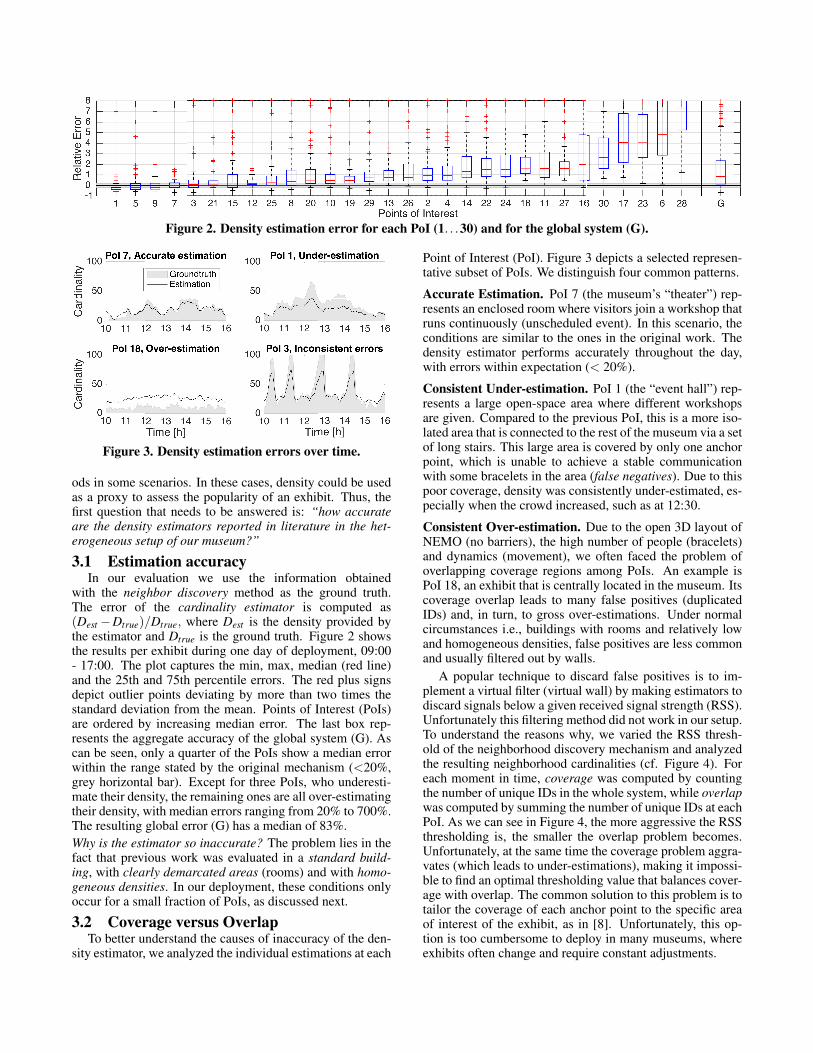
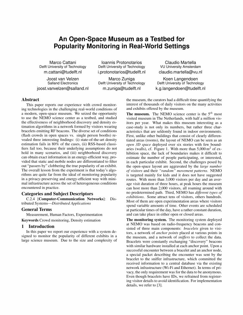
Figure 2. Density estimation error for each PoI (1. . .30) and for the global system (G).

Figure 3. Density estimation errors over time.

ods in some scenarios. In these cases, density could be usedas a proxy to assess the popularity of an exhibit. Thus, thefirst question that needs to be answered is: “how accurateare the density estimators reported in literature in the het-erogeneous setup of our museum?”

3.1 Estimation accuracyIn our evaluation we use the information obtained

with the neighbor discovery method as the ground truth.The error of the cardinality estimator is computed as(Dest −Dtrue)/Dtrue, where Dest is the density provided bythe estimator and Dtrue is the ground truth. Figure 2 showsthe results per exhibit during one day of deployment, 09:00- 17:00. The plot captures the min, max, median (red line)and the 25th and 75th percentile errors. The red plus signsdepict outlier points deviating by more than two times thestandard deviation from the mean. Points of Interest (PoIs)are ordered by increasing median error. The last box rep-resents the aggregate accuracy of the global system (G). Ascan be seen, only a quarter of the PoIs show a median errorwithin the range stated by the original mechanism (<20%,grey horizontal bar). Except for three PoIs, who underesti-mate their density, the remaining ones are all over-estimatingtheir density, with median errors ranging from 20% to 700%.The resulting global error (G) has a median of 83%.Why is the estimator so inaccurate? The problem lies in thefact that previous work was evaluated in a standard build-ing, with clearly demarcated areas (rooms) and with homo-geneous densities. In our deployment, these conditions onlyoccur for a small fraction of PoIs, as discussed next.

3.2 Coverage versus OverlapTo better understand the causes of inaccuracy of the den-

sity estimator, we analyzed the individual estimations at each

Point of Interest (PoI). Figure 3 depicts a selected represen-tative subset of PoIs. We distinguish four common patterns.

Accurate Estimation. PoI 7 (the museum’s “theater”) rep-resents an enclosed room where visitors join a workshop thatruns continuously (unscheduled event). In this scenario, theconditions are similar to the ones in the original work. Thedensity estimator performs accurately throughout the day,with errors within expectation (< 20%).

Consistent Under-estimation. PoI 1 (the “event hall”) rep-resents a large open-space area where different workshopsare given. Compared to the previous PoI, this is a more iso-lated area that is connected to the rest of the museum via a setof long stairs. This large area is covered by only one anchorpoint, which is unable to achieve a stable communicationwith some bracelets in the area (false negatives). Due to thispoor coverage, density was consistently under-estimated, es-pecially when the crowd increased, such as at 12:30.

Consistent Over-estimation. Due to the open 3D layout ofNEMO (no barriers), the high number of people (bracelets)and dynamics (movement), we often faced the problem ofoverlapping coverage regions among PoIs. An example isPoI 18, an exhibit that is centrally located in the museum. Itscoverage overlap leads to many false positives (duplicatedIDs) and, in turn, to gross over-estimations. Under normalcircumstances i.e., buildings with rooms and relatively lowand homogeneous densities, false positives are less commonand usually filtered out by walls.

A popular technique to discard false positives is to im-plement a virtual filter (virtual wall) by making estimators todiscard signals below a given received signal strength (RSS).Unfortunately this filtering method did not work in our setup.To understand the reasons why, we varied the RSS thresh-old of the neighborhood discovery mechanism and analyzedthe resulting neighborhood cardinalities (cf. Figure 4). Foreach moment in time, coverage was computed by countingthe number of unique IDs in the whole system, while overlapwas computed by summing the number of unique IDs at eachPoI. As we can see in Figure 4, the more aggressive the RSSthresholding is, the smaller the overlap problem becomes.Unfortunately, at the same time the coverage problem aggra-vates (which leads to under-estimations), making it impossi-ble to find an optimal thresholding value that balances cover-age with overlap. The common solution to this problem is totailor the coverage of each anchor point to the specific areaof interest of the exhibit, as in [8]. Unfortunately, this op-tion is too cumbersome to deploy in many museums, whereexhibits often change and require constant adjustments.

Figure 4. Coverage and overlap for different RSS values.

Inconsistent Estimation Errors. While for the previoustwo types of estimation errors it is possible to solve thecoverage/overlap problem with a careful and time consum-ing deployment, for exhibits with large coverage areas andhighly heterogeneous densities even a perfect positioningand filtering system would not reduce the inaccuracies.

This is the case for PoI 3 (the museum’s “chain reaction”show), which is the most famous exhibit in the museum, andspans from the first to the third floor of the building. Thisshow is repeated 5 times a day, lasts 15 minutes, and attractsa large fraction of the visitors around the internal balcony ofthe museum. As shown in Figure 3, the estimation is quiteaccurate during the time where there is no show (low homo-geneous density composed by people passing by), but duringthe show the density is heavily under-estimated.

This estimation error is not due to a coverage problem,but is an artifact of how estimators cope with sudden changesin density. The estimation process is sped up by averaginglocal estimates with neighboring ones, effectively increasingthe number of samples, in turn boosting convergence. An ad-verse effect is that this approach smooths the spatial densitypeaks, leading to under-estimation in denser areas (PoI 3)and over-estimation in sparser ones.

3.3 Effects of Crowd DynamicsWe now analyze the effect of crowds on the propagation

of radio signals. This analysis highlights the limitations ofdensity classifiers. Our deployment has 11 static bracelets.We used these bracelets, together with anchor nodes, to mon-itor the changes in radio signals throughout the day.

Figure 5 depicts the effect that density has on radio cov-erage and signal strength. Every 300 s, each static point(bracelet and anchor) calculated (i) the average density in itssurroundings, (ii) the average RSS from other static pointsand (iii) the average “radio range”. The average radio rangewas obtained as follows: upon receiving a packet from astatic point, the receiver calculated its distance to the sender(positions of static points are known), and averaged this dis-tance with all other distances observed during the last 300 s.The boxplots represent the averages during a day.Effects on Range. The results in Figure 5 (left) indicate thatan increase in crowd density reduces the maximum range ofdevices, while not significantly affecting the median. Thisis not too surprising, since people are known to cause signalattenuation due to body effects, which filters out weaker ra-dio signals sent by distant nodes. The result does indicate,however, that existing cardinality estimators are ill-equippedto calculate densities (number of devices over a given area),

5 15 25 35 45 55

Cardinality

-90

-80

-70

-60

RS

S [

db

m]

Signal Strength

5 15 25 35 45 55

Cardinality

0

20

40

60

Ra

ng

e [

m]

Radio Range

Figure 5. Effect of the crowd density on static nodes.

5 15 25 35 45 55-95

-85

-75

-65

RS

S [dbm

]

PoI 9, Positive

5 15 25 35 45 55-95

-85

-75

-65PoI 20, Negative

5 15 25 35 45 55

Cardinality

-95

-85

-75

-65

RS

S [dbm

] PoI 3, Mixed

5 15 25 35 45 55

Cardinality

-95

-85

-75

-65PoI 12, None

Figure 6. Effect of the crowd density on RSS.

since the radio range is oddly influenced by the crowd.Effects on Signal. According to many crowd density classi-fiers, when the crowd density increases, signal strength char-acteristics should get worse. Similar to what is hypothesizedfor radio range, the assumption is that an increasing num-ber of people should reduce the average RSS (due to bodyeffects) but increase its variance (due to multi-path effects).

Surprisingly, this relation does not hold for the RSS val-ues observed in our deployment. Figure 5 (right) shows noclear correlation between crowd density and key features inthe RSS (median and variance). To better understand whyour observations diverge from previous works, we analyzedthe relation between density and signal strength for each PoI.Figure 6 depicts a representative subset. Note that each PoIin this subset showcases a different relation.Negative correlation. PoI 9 (an open-space exhibit) hasa rather constant and homogeneous density throughout theday, cf. Figure 2. In this scenario, the relation between den-sity and RSS follows the assumption made in prior studies,with a decreasing median and a slightly increasing variance(except for density 55, for which we do not have enough datapoints to accurately compute the variance).Positive correlation. Surprisingly, even though PoI 20 rep-resents a scenario similar to PoI 9, its RSS values show theopposite relation with density. We do not know the exact rea-sons for this difference, but we hypothesize that it is causedby the different levels of interference perceived by the twoPoIs. Figure 2 shows indeed that PoI 20 is affected by morefalse positives than PoI 9. This implies that PoI 20 is exposedto more overlapping areas and long links, which increaseinterference. According to [1], this increased interferencecould lead to RSS values that are up to 8 dBm higher thannormal, an offset that is almost as big as the range observedin Figure 6.

Points of Interest (ordered by popularity)6 21 23 28 22 24 30 11 14 16 17 18 26 27 2 4 29 25 3 13 8 15 10 19 20 7 9 12 1 5 G

Car

dina

lity

01020304050

Static Nodes (popularity)Mobile NodesDensity Estimator

Figure 7. Breakdown of static and mobile nodes (neighborhood discovery) and the density estimates.

Figure 8. Density and popularity over time.

Inconsistent correlation. PoI 3 (the open-space “chain reac-tion” show) presents inconsistent behavior, with median RSSvalues that both increase and decrease with density. This bi-modal behavior is probably caused by the peculiar character-istics of this PoI, which periodically morphs from a point oftransit to a crowded point of attraction (and vice versa).No correlation. Finally, PoI 12 (a laboratory setting) fea-tures a limited number of participants, all seated and wellspaced from each other. In this scenario the crowd is sosparse and small that it does not affect the perceived signalstrength.As shown the relation between signal and density drasticallychanges depending on the scenario. Existing density clas-sifiers work only when assuming a uniform distribution thatdoes not change drastically over time. We argue that for suchclassifiers to work in heterogeneous scenarios, such as ourmuseum, PoIs would need to undergo cumbersome trainingto account for the peculiar radio features of each area.

4 Popularity AnalysisAs was shown in the previous section, density estimation

and classification techniques struggle with the heterogeneousset of conditions found in the museum, producing inaccurateresults in many cases. What is worse, in this section we willshow that density is a poor proxy for the popularity of anexhibit. The reason is that density does not discriminate vis-itors engaged with the exhibit’s activity from “passers by”that happen to be in the vicinity for a short while. This isespecially a concern in our test-case museum as the lack offixed routes (e.g., corridors) in combination with the open-space layout makes it hard to physically separate visitors andpassersby, which rules out the use of RSS thresholding tolimit the area of interest surrounding an exhibit. The conceptof an area of interest is also dynamic, as at busy times peoplequeue up in unpredictable ways.

The definition of popularity that we will be using through-out the remainder of the paper is the number of visitors thatstays in the vicinity of an anchor point for some time windowW . More formally, we distinguish Static (S) and Mobile (M)nodes:

S(i, t) =W⋂

w=0

nt−wi , M(i, t) = nt

i−S(i, t),

where nti is the neighborhood discovered by PoI i at time t.

The popularity of exhibit i at time t is then simply given by|S(i, t)|. We experimented with lengths of window W from10 to 300 seconds. As longer windows provide a smootherdisplay of changes over time, we will present the results fromthe largest window size (W = 300 s) in the sequel of the pa-per. With shorter windows, similar results were obtained.

The importance of properly discriminating static and mo-bile nodes can be seen in Figure 7, which plots the mediannumber of static (red bars) and mobile (yellow bars) nodesobserved with our neighborhood discovery data during a day.The higher the red bar, the more popular the PoI is. Note thatthe fraction of mobile nodes differs considerably betweenPoIs, and is uncorrelated with popularity. Overall, about halfthe nodes are mobile, and should be disregarded. For exam-ple, looking at the aggregated cardinality, PoI 3 would be thesecond most popular exhibit, while in fact it is only the 11th

most popular one (PoI 1 is the second most popular). For ref-erence, Figure 7 also includes the cardinalities produced bythe density estimator (black lines), showing that using themwould result in an even-more incorrect ordering of the popu-larity of the PoIs.

While Figure 7 presents the median cardinalities across awhole day, it is also instructive to look at how the fraction ofmobile nodes changes over time as interesting patterns canbe observed. Figure 8 plots the static/mobile breakdown forfour exemplary scenarios.Points of attraction. PoI 21 (the auditorium) is enclosed bywalls and features a periodic shows that attracts tens of vis-itor for a short, fixed period of time (grey bars in Figure 8).In these conditions the flow dynamics are minimal as peopleenter the room shortly before a show starts; note the minimalyellow shading at the left of each show. Consequently, den-sity estimations maps almost perfectly to popularity for theauditorium. PoI 8 (a small bar outside the auditorium) mon-itors visitors having a short snack (intended) as well as theones passing by (unintended) clobbering the real popularity.Point of passage. PoI 2, on the other hand, represents anexhibit located in an open space, close to a point of passagei.e., an area that is similar to a corridor but does not havewalls. In this case most of its perceived density it is due topeople passing by. To understand the popularity of PoIs likethis, it is therefore essential to distinguish between static and

dynamic neighboring bracelets, especially since the fractionof mobile nodes varies across time.Temporal hybrids. Finally, PoI 3 (the “chain reaction”) isnormally a popular point of passage (amidst several stair-cases, see Figure 1), but periodically becomes a point of at-traction for a short duration (show times are highlighted witha grey background). The error, i.e., the number of movingnodes taken into account, in this case drastically fluctuates,with rather accurate estimations during the periodic shows(hardly any yellow on top) and bad estimates during the re-maining periods (lots of yellow).

5 Fun FactsAlthough experimentation with a thousand devices comes

with a lot of hard work and frustration, the museum experi-ence also revealed some fun facts that kept us going.• Independently of the battery capacity, the lifetime of a

bracelet is just two days. We argue that this is due to the factthat kids like to use bracelets as swords.• Having a beaconing mechanism is useful when recover-

ing bracelets abandoned at the most unusual places i.e., plantpots and urinals.• Ethernet is not as reliable as WiFi; wall sockets can easily

be powered down by technicians heading home at 5PM.

6 Conclusions and Future DirectionsThis paper reported our experience in monitoring the pop-

ularity of exhibits in a modern, open-space science museum.We equipped visitors with bracelets emitting RF beacons, al-lowing us to study crowd-monitoring mechanisms such asneighbor discovery algorithms, cardinality estimators, anddensity classifiers in a diverse set of real-world settings.

An in-depth analysis of the collected data (proximity de-tections and density estimations) provided a better under-standing of the limitations of the existing mechanisms. Inparticular, the use of ID-based neighbor discovery allowed usto univocally associate each bracelet to the point of interest,and distinguish static from mobile nodes. The latter provedkey to understanding the relation between density and pop-ularity. Cardinality estimators and density classifiers cannotprovide such differentiation, resulting in estimation errors farhigher than originally reported (more than 20% error in 80%of the cases). We argue that these mechanism could be eas-ily improved by letting bracelets sense their mobility, e.g.with accelerometers, or by letting anchor points exchangeinformation and distributedly disambiguate each bracelet. Inthe case of density classifiers, similar improvements couldbe achieved by developing more complex models capable ofdifferentiating their estimations based on the application sce-nario (open-space, rooms, ...). An important line of futureresearch is thus to devise lightweight and privacy-preservingcrowd-monitoring algorithms that can univocally associateeach person to a single anchor point while differentiating be-tween static and mobile visitor. Only in this way one willable to provide a precise estimation of popularity.

7 AcknowledgmentsWe would like to thank the anonymous reviewers and our

shepherd Yuan He for providing us detailed feedback ondraft versions of this paper. This work was supported by

the Dutch national program COMMIT/ (project P09EWiDS)and NEMO’s Science Live research program.

8 References[1] A. Behboodi, N. Wirstrom, F. Lemic, T. Voigt, and A. Wolisz. In-

terference effect on localization solutions: Signal feature perspective.IEEE Vehicular Technology Conference, 2015.

[2] E. Bruns, B. Brombach, T. Zeidler, and O. Bimber. Enabling mobilephones to support large-scale museum guidance. IEEE Multimedia,(2):16–25, 2007.

[3] M. Cattani. Opportunistic Communication in Extreme Wireless SensorNetworks. PhD thesis, Delft University of Technology, 2016.

[4] M. Cattani, M. Zuniga, A. Loukas, and K. G. Langendoen.Lightweight Cardinality Estimation in Dynamic Wireless Networks.In 13th ACM/IEEE Int. Conf. on Information Processing in SensorNetworks (IPSN), pages 179–189, 2014.

[5] V. Iyer, A. Pruteanu, and S. Dulman. NetDetect: Neighborhood Dis-covery in Wireless Networks Using Adaptive Beacons. In 5th Int.Conf. on Self-Adaptive and Self-Organizing Systems, pages 31–40, oct2011.

[6] J. Lanir, P. Bak, and T. Kuflik. Visualizing proximity-based spatiotem-poral behavior of museum visitors using tangram diagrams. In Com-puter Graphics Forum, volume 33, pages 261–270. Wiley Online Li-brary, 2014.

[7] C. Martella, M. Dobson, A. V. Halteren, and M. van Steen. Fromproximity sensing to spatio-temporal social graphs. In IEEE Int. Conf.on Pervasive Computing and Communications (PerCom), pages 78–87, 2014.

[8] C. Martella, A. Miraglia, M. Cattani, and M. V. Steen. LeveragingProximity Sensing to Mine the Behavior of Museum Visitors. InIEEE Int.Conf. on Pervasive Computing and Communications (Per-Com), 2016.

[9] C. Martella, M. van Steen, A. Halteren, C. Conrado, and J. Li.Crowd textures as proximity graphs. IEEE Communications Maga-zine, 52(1):114–121, 2014.

[10] M. Nakatsuka, H. Iwatani, and J. Katto. A Study on Passive CrowdDensity Estimation using Wireless Sensors. 4th Intl. Conf. on MobileComputing and Ubiquitous Networking (ICMU), (2):1–6, 2008.

[11] C. Qian, H. Ngan, Y. Liu, and L. Ni. Cardinality Estimation for Large-Scale RFID Systems. IEEE transactions on parallel and distributedsystems, 22(9):1441–1454, 2011.

[12] A. J. Ruiz-Ruiz, H. Blunck, T. S. Prentow, A. Stisen, and M. B. Kjaer-gaard. Analysis methods for extracting knowledge from large-scalewifi monitoring to inform building facility planning. In IEEE Int.Conf. on Pervasive Computing and Communications (PerCom), pages130–138, 2014.

[13] R. Strohmaier, G. Sprung, A. Nischelwitzer, and S. Schadenbauer. Us-ing visitor-flow visualization to improve visitor experience in muse-ums and exhibitions. In Museums and the Web (MW2015), 2015.

[14] J. Weppner and P. Lukowicz. Collaborative crowd density estimationwith mobile phones. In 3rd Int. Workshop on Sensing Applications onMobile Phones (PhoneSens), 2011.

[15] J. Weppner and P. Lukowicz. Bluetooth based collaborative crowddensity estimation with mobile phones. In IEEE Conf. on PervasiveComputing and Communications (PerCom), pages 193–200, 2013.

[16] G. Wilson. Multimedia tour programme at tate modern. In Museumsand the Web, volume 3, 2004.

[17] Y. Yoshimura, F. Girardin, J. P. Carrascal, C. Ratti, and J. Blat. Newtools for studying visitor behaviours in museums: a case study at thelouvre. In Int. Conf. on Information and Communication Technologiesin Tourism (ENTER 2012), pages 391–402, 2012.

[18] C.-W. You, C.-C. Wei, Y.-L. Chen, H.-H. Chu, and M.-S. Chen. Usingmobile phones to monitor shopping time at physical stores. IEEEPervasive Computing, 10(2):37–43, 2011.

[19] Y. Yuan, C. Qiu, W. Xi, and J. Zhao. Crowd Density Estimation UsingWireless Sensor Networks. In Int. Conf. on Mobile Ad-hoc and SensorNetworks, pages 138–145, 2011.

[20] Y. Yuan, J. Zhao, C. Qiu, and W. Xi. Estimating Crowd Den-sity in an RF-Based Dynamic Environment. IEEE Sensors Journal,13(10):3837–3845, 2013.