![Old Fashioned - 2nd issue [topics]](https://static.fdocuments.net/doc/165x107/568bdefd1a28ab2034bb7a98/old-fashioned-2nd-issue-topics.jpg)
An Old-Fashioned Recipe for Real Time - Microsoft Research
53
An Old-Fashioned Recipe for Real Time Mart´ ın Abadi and Leslie Lamport Wed 22 Dec PST 1993 [17:32] This body of this paper appeared in ACM Transactions on Pro- gramming Languages and Systems 16, 5 (September 1994) 1543– 1571. The appendix was published electronically by the ACM.
Transcript of An Old-Fashioned Recipe for Real Time - Microsoft Research

An Old-Fashioned Recipe for Real Time
Mart́ın Abadi and Leslie Lamport
Wed 22 Dec PST 1993 [17:32]
This body of this paper appeared in ACM Transactions on Pro-gramming Languages and Systems 16, 5 (September 1994) 1543–1571. The appendix was published electronically by the ACM.

Contents
1 Introduction 1543
2 Closed Systems 15452.1 The Lossy-Queue Example . . . . . . . . . . . . . . . . . . . . . . . 15452.2 The Semantics of TLA . . . . . . . . . . . . . . . . . . . . . . . . . . 15482.3 Safety and Fairness . . . . . . . . . . . . . . . . . . . . . . . . . . . . 15492.4 History-Determined Variables . . . . . . . . . . . . . . . . . . . . . . 1551
3 Real-Time Closed Systems 15523.1 Time and Timers . . . . . . . . . . . . . . . . . . . . . . . . . . . . . 15523.2 Reasoning About Time . . . . . . . . . . . . . . . . . . . . . . . . . . 15543.3 The NonZeno Condition . . . . . . . . . . . . . . . . . . . . . . . . . 15573.4 An Example: Fischer’s Protocol . . . . . . . . . . . . . . . . . . . . . 1560
4 Open Systems 15624.1 Receptiveness and Realizability . . . . . . . . . . . . . . . . . . . . . 15624.2 The −� Operator . . . . . . . . . . . . . . . . . . . . . . . . . . . . . 15634.3 Proving Machine Realizability . . . . . . . . . . . . . . . . . . . . . . 15634.4 Reduction to Closed Systems . . . . . . . . . . . . . . . . . . . . . . 15644.5 Composition . . . . . . . . . . . . . . . . . . . . . . . . . . . . . . . 1564
5 Real-Time Open Systems 15655.1 A Paradox . . . . . . . . . . . . . . . . . . . . . . . . . . . . . . . . . 15655.2 Timing Constraints in General . . . . . . . . . . . . . . . . . . . . . 1568
6 Conclusion 15696.1 What We Did . . . . . . . . . . . . . . . . . . . . . . . . . . . . . . . 15696.2 Beyond Real Time . . . . . . . . . . . . . . . . . . . . . . . . . . . . 1570
A Definitions A–1A1 States and Behaviors . . . . . . . . . . . . . . . . . . . . . . . . . . . A–1A2 Predicates and Actions . . . . . . . . . . . . . . . . . . . . . . . . . . A–1A3 Properties . . . . . . . . . . . . . . . . . . . . . . . . . . . . . . . . . A–1A4 Closure and Safety . . . . . . . . . . . . . . . . . . . . . . . . . . . . A–2A5 Realizability . . . . . . . . . . . . . . . . . . . . . . . . . . . . . . . . A–2
B Proofs A–2B1 Proof Notation . . . . . . . . . . . . . . . . . . . . . . . . . . . . . . A–2B2 Proof of Proposition 2 . . . . . . . . . . . . . . . . . . . . . . . . . . A–3B3 Proof of Proposition 3 . . . . . . . . . . . . . . . . . . . . . . . . . . A–4B4 Two Lemmas About Machine-Realizability . . . . . . . . . . . . . . A–4B5 Proof of Proposition 4 . . . . . . . . . . . . . . . . . . . . . . . . . . A–5B6 Proof of Proposition 5 . . . . . . . . . . . . . . . . . . . . . . . . . . A–9B7 Proof of Theorem 4 . . . . . . . . . . . . . . . . . . . . . . . . . . . . A–10
B7.1 High-Level Proof of the Theorem . . . . . . . . . . . . . . . . A–10B7.2 Detailed Proof of the Theorem . . . . . . . . . . . . . . . . . A–13
Index A–21

An Old-Fashioned Recipe for Real Time
MART́IN ABADI and LESLIE LAMPORT
Digital Equipment Corporation
Traditional methods for specifying and reasoning about concurrent systems work for real-timesystems. Using TLA (the temporal logic of actions), we illustrate how they work with the examplesof a queue and of a mutual-exclusion protocol. In general, two problems must be addressed:avoiding the real-time programming version of Zeno’s paradox, and coping with circularities whencomposing real-time assumption/guarantee specifications. Their solutions rest on properties ofmachine closure and realizability.
Categories and Subject Descriptors: D.2.4 [Software Engineering]: Program Verification—correctness proofs; F.3.1 [Logics and Meanings of Programs]: Specifying and Verifying andReasoning about Programs—Specification techniques
General Terms: Theory, Verification
Additional Key Words and Phrases: Composition, concurrent programming, liveness properties,real time, safety properties, temporal logic, Zeno
1. INTRODUCTION
A new class of systems is often viewed as an opportunity to invent a new semantics.A number of years ago, the new class was distributed systems. More recently,it has been real-time systems. The proliferation of new semantics may be funfor semanticists, but developing a practical method for reasoning formally aboutsystems is a lot of work. It would be unfortunate if every new class of systemsrequired inventing new semantics, along with proof rules, languages, and tools.Fortunately, no fundamental change to the old methods for specifying and rea-
soning about systems is needed for these new classes. It has long been known thatthe methods originally developed for shared-memory multiprocessing apply equallywell to distributed systems [Chandy and Misra 1988; Lamport 1982]. The firstapplication we have seen of a clearly “off-the-shelf” method to a real-time algo-rithm was in 1983 [Neumann and Lamport 1983], but there were probably earlierones. Indeed, the “extension” of an existing temporal logic to real-time programsby Bernstein and Harter [1981] can be viewed as an application of that logic.The old-fashioned methods handle real time by introducing a variable, which we
call now, to represent time. This idea is so simple and obvious that it seems hardly
Author’s address: Systems Research Center, Digital Equipment Corporation, 130 Lytton Avenue,Palo Alto, CA 94301.Permission to copy without fee all or part of this material is granted provided that the copies arenot made or distributed for direct commercial advantage, the ACM copyright notice and the titleof the publication and its date appear, and notice is given that copying is by permission of the
Association for Computing Machinery. To copy otherwise, or to republish, requires a fee and/orspecific permission.c© 1993 ACM 0000-0000/93/0000-0000 $00.00
ACM Transactions on Programming Languages and Systems, Vol ? No. ?, November 1993, Pages 1543–1571.

1544 · Mart́ın Abadi and Leslie Lamport
worth writing about, except that few people appear to be aware that it works inpractice. We therefore describe how to apply a conventional method to real-timesystems.Any formalism for reasoning about concurrent programs can be used to prove
properties of real-time systems. However, in a conventional formalism based ona programming language, real-time assumptions are expressed by adding programoperations that read and modify the variable now . The result can be a complicatedprogram that is hard to understand and easy to get wrong. We take as our for-malism TLA, the temporal logic of actions [Lamport 1991]. In TLA, programs andproperties are represented as logical formulas. A real-time program can be writtenas the conjunction of its untimed version, expressed in a standard way as a TLAformula, and its timing assumptions, expressed in terms of a few standard param-eterized formulas. This separate specification of timing properties makes real-timespecifications easier to write and understand.The method is illustrated with two examples. The first is a queue in which
the sender and receiver synchronize by the use of timing assumptions instead ofacknowledgements. We indicate how safety and liveness properties of the queuecan be proved. The second example is an n-process mutual exclusion protocol, inwhich mutual exclusion depends on assumptions about the length of time taken bythe operations. Its correctness is proved by a conventional invariance argument.We also discuss two problems that arise when time is represented as a program
variable—problems that seem to have received little attention—and present newsolutions.The first problem is how to avoid the real-time programming version of Zeno’s
paradox. If time becomes an ordinary program variable, then one can inadvertentlywrite programs in which time behaves improperly. An obvious danger is deadlock,where time stops. A more insidious possibility is that time keeps advancing butis bounded, approaching closer and closer to some limit. One way to avoid such“Zeno” behaviors is to place an a priori lower bound on the duration of any action,but this can complicate the representation of some systems. We provide a moregeneral and, we feel, a more natural solution.The second problem is coping with the circularity that arises in open system spec-
ifications. The specification of an open system asserts that it operates correctlyunder some assumptions on the system’s environment. A modular specificationmethod requires a rule asserting that, if each component satisfies its specification,then it behaves correctly in concert with other components. This rule is circular,because a component’s specification requires only that it behave correctly if its en-vironment does, and its environment consists of all the other components. Despiteits circularity, the rule is sound for specifications written in a particular style [Abadiand Lamport 1993; Misra and Chandy 1981; Pnueli 1984]. By examining an appar-ently paradoxical example, we discover how real-time specifications of open systemscan be written in this style.We express these problems and their solutions in terms of TLA. However, we
believe that the problems will arise in any formalism that permits sufficiently gen-eral specifications. Our solutions should be applicable to any formalism whosesemantics is based on sequences of states or actions.
ACM Transactions on Programming Languages and Systems, Vol ?, No. ?, November 1993.

An Old-Fashioned Recipe for Real Time · 1545
2. CLOSED SYSTEMS
We briefly review how to represent closed systems in TLA. A closed system isone that is self-contained and does not communicate with an environment. Noone intentionally designs autistic systems; in a closed system, the environment isrepresented as part of the system. Open systems, in which the environment andsystem are separated, are discussed in Section 4.We begin our review of TLA in Section 2.1 with an informal presentation of an
example. The formal definitions are summarized in Section 2.2. A more leisurelyexposition appears in [Lamport 1991], and most definitions in the current paper arerepeated in a list in the appendix. Section 2.3 reviews the concepts of safety [Alpernand Schneider 1985] and machine closure [Abadi and Lamport 1991] (also known asfeasibility [Apt, Francez, and Katz 1988]) and relates them to TLA, and Section 2.4defines a useful class of history variables [Abadi and Lamport 1991]. Propositionsand theorems are proved in the appendix.
2.1 The Lossy-Queue Example
We introduce TLA with the example of the lossy queue shown in Figure 1. Theinterface consists of two pairs of “wires”, each pair consisting of a val wire thatholds a message and a boolean-valued bit wire. A message m is sent over a pair ofwires by setting the val wire to m and complementing the bit wire. The receiverdetects the presence of a new message by observing that the bit wire has changedvalue. Input to the queue arrives on the wire pair (ival , ibit), and output is senton the wire pair (oval , obit). There is no acknowledgment protocol, so inputs arelost if they arrive faster than the queue processes them. (Because of the way ibitis used, inputs are lost in pairs.) The property guaranteed by this lossy queue isthat the sequence of output messages is a subsequence of the sequence of inputmessages. In Section 3.1, we add timing constraints to rule out the possibility oflost messages.A specification is a TLA formula Π describing a set of allowed behaviors. A
property P is also a TLA formula. The specification Π satisfies property P iff (ifand only if) every behavior allowed by Π is also allowed by P—that is, if Π impliesP . Similarly, a specification Ψ implements Π iff every behavior allowed by Ψ is alsoallowed by Π, so implementation means implication.The specification of the lossy queue is a TLA formula that mentions the four
variables ibit , obit , ival , and oval , as well as two internal variables: q, which equals
✲
✲
✲
✲
ibit
ival
obit
ovalq: . . .
last :
Fig. 1. A simple queue.
ACM Transactions on Programming Languages and Systems, Vol ?, No. ?, November 1993.

1546 · Mart́ın Abadi and Leslie Lamport
InitQ∆= ∧ ibit , obit ∈ {true, false}
∧ ival , oval ∈ Msg∧ last = ibit∧ q = 〈〈〉〉
Inp∆= ∧ ibit ′ = ¬ibit
∧ ival ′ ∈ Msg∧ (obit , oval , q, last)′ = (obit , oval , q, last)
EnQ∆= ∧ last = ibit
∧ q′ = q ◦ 〈〈ival〉〉∧ last ′ = ibit∧ (ibit , obit , ival , oval)′ = (ibit , obit , ival , oval)
DeQ∆= ∧ q = 〈〈〉〉
∧ oval ′ = Head(q)∧ q′ = Tail(q)∧ obit ′ = ¬obit∧ (ibit , ival , last)′ = (ibit, ival , last)
NQ∆= Inp ∨ EnQ ∨ DeQ
v∆= (ibit , obit , ival , oval , q, last)
ΠQ∆= InitQ ∧ ✷[NQ]v
ΦQ∆= ∃∃∃∃∃∃q, last : ΠQ
Fig. 2. The TLA specification of a lossy queue.
the sequence of messages received but not yet output; and last , which equals thevalue of ibit for the last received message. (The variable last is used to prevent thesame message from being received twice.) These six variables are flexible variables;their values can change during a behavior. We also introduce a rigid variable Msgdenoting the set of possible messages; it has the same value throughout a behavior.We usually refer to flexible variables simply as variables, and to rigid variables asconstants.The TLA specification is shown in Figure 2, using the following notation. A
list of formulas, each prefaced by ∧, denotes the conjunction of the formulas, andindentation is used to eliminate parentheses. The expression 〈〈 〉〉 denotes the emptysequence, 〈〈m〉〉 denotes the singleton sequence having m as its one element, ◦denotes concatenation, Head(σ) denotes the first element of σ, and Tail(σ) denotesthe sequence obtained by removing the first element of σ. The symbol ∆= means isdefined to equal.The first definition is of the predicate InitQ, which describes the initial state. This
predicate asserts that the values of variables ibit and obit are arbitrary booleans,the values of ival and oval are elements of Msg, the values of last and ibit are equal,and the value of q is the empty sequence.Next is defined the action Inp, which describes all state changes that represent
the sending of an input message. (Since this is the specification of a closed system,it includes the environment’s Inp action.) The first conjunct, ibit ′ = ¬ibit , assertsthat the new value of ibit equals the complement of its old value. The second con-junct asserts that the new value of ival is an element of Msg. The third conjunct
ACM Transactions on Programming Languages and Systems, Vol ?, No. ?, November 1993.

An Old-Fashioned Recipe for Real Time · 1547
asserts that the value of the four-tuple (obit , oval , q, last) is unchanged; it is equiv-alent to the assertion that the value of each of the four variables obit , oval , q, andlast is unchanged. The action Inp is always enabled, meaning that, in any state, anew input message can be sent.Action EnQ represents the receipt of a message by the system. The first conjunct
asserts that last is not equal to ibit , so the message on the input wire has not yetbeen received. The second conjunct asserts that the new value of q equals thesequence obtained by concatenating the old value of ival to the end of q’s old value.The third conjunct asserts that the new value of last equals the old value of ibit .The final conjunct asserts that the values of ibit , obit , ival , and oval are unchanged.Action EnQ is enabled in a state iff the values of last and ibit in that state areunequal.The action DeQ represents the operation of removing a message from the head
of q and sending it on the output wire. It is enabled iff the value of q is not theempty sequence.The action NQ is the specification’s next-state relation. It describes all allowed
changes to the queue system’s variables. Since the only allowed changes are theones described by the actions Inp, EnQ , and DeQ , action NQ is the disjunction ofthose three actions.In TLA specifications, it is convenient to give a name to the tuple of all relevant
variables. Here, we call it v.Formula ΠQ is the internal specification of the lossy queue—the formula spec-
ifying all sequences of values that may be assumed by the queue’s six variables,including the internal variables q and last . Its first conjunct asserts that InitQis true in the initial state. Its second conjunct, ✷[NQ]v, asserts that every stepis either an NQ step (a state change allowed by NQ) or else leaves v unchanged,meaning that it leaves all six variables unchanged.Formula ΦQ is the actual specification, in which the internal variables q and
last have been hidden. A behavior satisfies ΦQ iff there is some way to assignsequences of values to q and last such that ΠQ is satisfied. The free variables of ΦQ
are ibit , obit , ival , and oval , so ΦQ specifies what sequences of values these fourvariables can assume. All the preceding definitions just represent one possible wayof structuring the definition of ΦQ; there are infinitely many ways to write formulasthat are equivalent to ΦQ and are therefore equivalent specifications.TLA is an untyped logic; variables may assume any values in a fixed universal
domain. Type correctness can be expressed by the formula ✷T , where T is thepredicate asserting that all relevant variables have values of the expected “types”.For the internal queue specification, the type-correctness predicate is
TQ∆= ∧ ibit , obit , last ∈ {true, false}∧ ival , oval ∈ Msg∧ q ∈ Msg∗
(1)
where Msg∗ is the set of finite sequences of messages. Type correctness of ΠQ isasserted by the formula ΠQ ⇒ ✷TQ, which is easily proved [Lamport 1991]. Typecorrectness of ΦQ follows from ΠQ ⇒ ✷TQ by the usual rules for reasoning aboutquantifiers.Formulas ΠQ and ΦQ are safety properties, meaning that they are satisfied by
ACM Transactions on Programming Languages and Systems, Vol ?, No. ?, November 1993.

1548 · Mart́ın Abadi and Leslie Lamport
an infinite behavior iff they are satisfied by every finite initial portion of the be-havior. Safety properties allow behaviors in which a system performs properly fora while and then the values of all variables are frozen, never to change again. Inasynchronous systems, such undesirable behaviors are ruled out by adding fairnessproperties. We could strengthen our lossy-queue specification by conjoining theweak fairness property WFv(DeQ) and the strong fairness property SFv(EnQ) toΠQ, obtaining
∃∃∃∃∃∃ q, last : (InitQ ∧ ✷[NQ]v ∧ WFv(DeQ) ∧ SFv(EnQ)) (2)
Property WFv(DeQ) asserts that if action DeQ is enabled forever, then infinitelymany DeQ steps must occur. This property implies that every message reachingthe queue is eventually output. Property SFv(EnQ) asserts that if action EnQ isenabled infinitely often, then infinitely many EnQ steps must occur. It impliesthat if infinitely many inputs are sent, then the queue must receive infinitely manyof them. The formula (2) implies the liveness property [Alpern and Schneider1985] that an infinite number of inputs produces an infinite number of outputs. Aformula such as (2), which is the conjunction of an initial predicate, a term of theform ✷[A]f , and a fairness property, is said to be in canonical form.2.2 The Semantics of TLA
We begin with some definitions. We assume a universal domain of values, and welet [[F ]] denote the semantic meaning of a formula F .
state. A mapping from variables to values. We let s.x denote the value that states assigns to variable x.state function. An expression formed from variables, constants, and operators.
The meaning of a state function is a mapping from states to values. For example,x+ 1 is a state function such that [[x + 1]](s) equals s.x+ 1, for any state s.predicate. A boolean-valued state function, such as x > y + 1.transition function. An expression formed from variables, primed variables, con-
stants, and operators. The meaning of a transition function is a mapping from pairsof states to values, with unprimed variables referring to the first state of a pair andprimed variables to the second. For example, x + y′ + 1 is a transition function,and [[x + y′ + 1]](s, t) equals the value s.x+ t.y + 1, for any pair of states s, t.action. A boolean-valued transition function, such as x > (y′ + 1).step. A pair of states s, t. For an action A, the pair is called an A step iff [[A]](s, t)
equals true. It is called a stuttering step iff s = t.f ′. The transition function obtained from the state function f by priming all the
free variables of f , so [[f ′]](s, t) = [[f ]](t) for any states s and t.[A]f . The action A ∨ (f ′ = f), for any action A and state function f .〈A〉f . The action A∧ (f ′ �= f), for any action A and state function f .Enabled A. For any action A, the predicate such that [[Enabled A]](s) equals
∃t : [[A]](s, t), for any state s.Informally, we often identify a formula and its meaning. For example we say thata predicate P is true in state s instead of [[P ]](s) = true.
ACM Transactions on Programming Languages and Systems, Vol ?, No. ?, November 1993.

An Old-Fashioned Recipe for Real Time · 1549
An RTLA (raw TLA) formula is a boolean expression built from actions, classicaloperators (boolean operators and quantification over rigid variables), and the unarytemporal operator ✷. The meaning of an RTLA formula is a boolean-valued func-tion on behaviors, where a behavior is an infinite sequence of states. The meaningof the operator ✷ is defined by
[[✷F ]](s1, s2, s3, . . .)∆= ∀n > 0 : [[F ]](sn, sn+1, sn+2, . . .)
Intuitively, ✷F asserts that F is always true. The meaning of an action as an RTLAformula is defined in terms of its meaning as an action by letting [[A]](s1, s2, s3, . . .)equal [[A]](s1, s2). A predicate P is an action; P is true for a behavior iff it is truefor the first state of the behavior, and ✷P is true iff P is true in all states. For anyaction A and state function f , the formula ✷[A]f is true for a behavior iff each stepis an A step or else leaves f unchanged. The classical operators have their usualmeanings.A TLA formula is one that can be constructed from predicates and formulas
✷[A]f using classical operators, ✷, and existential quantification over flexible vari-ables. Thus, an action that is not a predicate can appear in a TLA formula Fonly as a subformula of an action A in a subformula ✷[A]f or Enabled A of F .The semantics of actions, classical operators, and ✷ are defined as before. Theapproximate meaning of quantification over a flexible variable is that ∃∃∃∃∃∃x : F is truefor a behavior iff there is some sequence of values that can be assigned to x thatmakes F true. The precise definition appears in [Lamport 1991] and is recalled inthe appendix. As usual, we write ∃∃∃∃∃∃x1, . . . , xn : F instead of ∃∃∃∃∃∃x1 : . . . ∃∃∃∃∃∃xn : F .A property is a set of behaviors that is invariant under stuttering, meaning that
it contains a behavior σ iff it contains every behavior obtained from σ by addingand/or removing stuttering steps. The set of all behaviors satisfying a TLA formulais a property, which we often identify with the formula.For any TLA formula F , action A, and state function f :
✸F∆= ¬✷¬F
WFf (A) ∆= ✷✸¬(Enabled 〈A〉f ) ∨ ✷✸〈A〉fSFf (A) ∆= ✸✷¬(Enabled 〈A〉f ) ∨ ✷✸〈A〉f
These are TLA formulas, since ✸〈A〉f equals ¬✷[¬A]f .2.3 Safety and Fairness
A finite behavior is a finite sequence of states. We say that a finite behavior satisfiesa property F iff it can be continued to an infinite behavior in F . A property F isa safety property [Alpern and Schneider 1985] iff the following condition holds: Fcontains a behavior iff it is satisfied by every finite prefix of the behavior.1 Intu-itively, a safety property asserts that something “bad” does not happen. Predicatesand formulas of the form ✷[A]f are safety properties.Safety properties are closed sets in a topology on the set of all behaviors [Abadi
and Lamport 1991]. Hence, if two TLA formulas F and G are safety properties,
1One sometimes defines s1, . . . , sn to satisfy F iff the behavior s1, . . . , sn, sn, sn, . . . is in F . Sinceproperties are invariant under stuttering, this alternative definition leads to the same definitionof a safety property.
ACM Transactions on Programming Languages and Systems, Vol ?, No. ?, November 1993.

1550 · Mart́ın Abadi and Leslie Lamport
then F ∧ G is also a safety property. The closure C(F ) of a property F is thesmallest safety property containing F . It can be shown that C(F ) is expressible inTLA, for any TLA formula F .If Π is a safety property and L an arbitrary property, then the pair (Π, L) is
machine closed iff every finite behavior satisfying Π can be extended to an infinitebehavior in Π ∧ L. Two equivalent definitions are that (Π, L) is machine closed iff(i) C(Π ∧ L) equals Π, or (ii) for any safety property Ψ, if Π ∧ L implies Ψ then Πimplies Ψ. The lack of machine closure can be a source of incompleteness for proofmethods. Most methods for proving safety properties use only safety properties ashypotheses, so they can prove Π ∧ L ⇒ Ψ for safety properties Π and Ψ only byproving Π⇒ Ψ. If Π is not machine closed, then Π∧L⇒ Ψ could hold even thoughΠ⇒ Ψ does not, and these methods will be unable to prove that the system withspecification Π satisfies Ψ.Proposition 1 below shows that machine closure generalizes the concept of fair-
ness. The canonical form for a TLA formula is
∃∃∃∃∃∃x : (Init ∧ ✷[N ]v ∧ L) (3)
where Init is a predicate, N is an action, v is a state function, L is a formula,(Init ∧✷[N ]v, L) is machine closed, and x is a tuple of variables called the internalvariables of the formula. Usually, v will be the tuple of all variables appearing freein Init , N , and L (including the variables of x). It follows from the definitionsthat a behavior satisfies (3) iff there is some way of choosing values for x such that(a) Init is true in the initial state, (b) every step is either an N step or leaves allthe variables in v unchanged, and (c) the entire behavior satisfies L.An action A is said to be a subaction of a safety property Π iff, whenever an
A step is possible, an A step that satisfies Π is possible. More precisely, A is asubaction of Π iff for every finite behavior s1, . . . , sn satisfying Π with Enabled Atrue in state sn, there exists a state sn+1 such that (sn, sn+1) is an A step ands1, . . . , sn+1 satisfies Π. By this definition, if A implies N then A is a subaction ofInit ∧ ✷[N ]v. The exact condition is that A is a subaction of Init ∧✷[N ]v iff2
Init ∧✷[N ]v ⇒ ✷((Enabled A)⇒ Enabled (A ∧ [N ]v))Two actions are disjoint iff their conjunction is identically false. A weaker notion isdisjointness of two actions for a property: A and B are disjoint for Π iff no behaviorsatisfying Π contains an A ∧ B step. By this definition, A and B are disjoint forInit ∧ ✷[N ]v iff
Init ∧ ✷[N ]v ⇒ ✷¬Enabled (A ∧ B ∧ [N ]v)The following result shows that the conjunction of WF and SF formulas is a
fairness property. It is a special case of Proposition 4 of Section 4.
Proposition 1. If Π is a safety property and L is the conjunction of a finite orcountably infinite number of formulas of the form WFw(A) and/or SFw(A) suchthat each 〈A〉w is a subaction of Π, then (Π, L) is machine closed.
2We let ⇒ have lower precedence than the other boolean operators.
ACM Transactions on Programming Languages and Systems, Vol ?, No. ?, November 1993.

An Old-Fashioned Recipe for Real Time · 1551
In practice, each w will usually be a tuple of variables changed by the correspondingaction A, so 〈A〉w will equal A.3 In the informal exposition, we often omit thesubscript and talk about A when we really mean 〈A〉w.Machine closure for more general classes of properties can be proved with the
following two propositions, which are proved in the appendix. To apply the first,one must prove that ∃∃∃∃∃∃x : Π is a safety property. By Proposition 2 of [Abadi andLamport 1991, page 265], it suffices to prove that Π has finite internal nondeter-minism (fin), with x as its internal state component. Here, fin means roughly thatthere are only a finite number of sequences of values for x that can make a finitebehavior satisfy Π.
Proposition 2. If (Π, L) is machine closed, x is a tuple of variables that donot occur free in L, and ∃∃∃∃∃∃x : Π is a safety property, then ((∃∃∃∃∃∃x : Π), L) is machineclosed.
Proposition 3. If (Π, L1) is machine closed and Π ∧ L1 implies L2, then(Π, L2) is machine closed.
2.4 History-Determined Variables
A history-determined variable is one whose current value can be inferred from thecurrent and past values of other variables. For the precise definition, let
Hist(h, f, g, v) ∆= (h = f) ∧ ✷[(h′ = g) ∧ (v′ �= v)](h,v) (4)
where f and v are state functions and g is a transition function. A variable h is ahistory-determined variable for a formula Π iff Π implies Hist(h, f, g, v), for somef , g, and v such that h occurs free in neither f nor v, and h′ does not occur free ing.If f and v do not depend on h, and g does not depend on h′, then ∃∃∃∃∃∃h :
Hist(h, f, g, v) is true for all behaviors. Therefore, if h does not occur free in formulaΦ, then ∃∃∃∃∃∃h : (Φ ∧ Hist(h, f, g, v)) is equivalent to Φ. In other words, conjoiningHist(h, f, g, v) to Φ does not change the behavior of its variables, so it makes h a“dummy variable” for Φ—in fact, it is a special kind of history variable [Abadi andLamport 1991, page 270].As an example, we add to the lossy queue’s specification ΦQ a history variable
hin that records the sequence of values transmitted on the input wire. Let
Hin∆= ∧ hin = 〈〈 〉〉∧ ✷[ ∧ hin ′ = hin ◦ 〈〈ival ′〉〉
∧ (ival , ibit)′ �= (ival , ibit) ](hin,ival,ibit)
(5)
Then Hin equals Hist(hin , 〈〈 〉〉, hin ◦ 〈〈ival ′〉〉, (ival , ibit)); therefore, hin is a history-determined variable for ΦQ ∧Hin , and ∃∃∃∃∃∃ hin : (ΦQ ∧Hin) equals ΦQ.If h is a history-determined variable for a property Π, then Π is fin, with h as
its internal state component. Hence, if Π is a safety property, then ∃∃∃∃∃∃h : Π is also asafety property.
3More precisely, T ∧ A will imply w′ = w, where T is the type-correctness invariant.
ACM Transactions on Programming Languages and Systems, Vol ?, No. ?, November 1993.

1552 · Mart́ın Abadi and Leslie Lamport
3. REAL-TIME CLOSED SYSTEMS
We now use TLA to specify and reason about timing properties of closed systems.We focus on worst-case upper and lower bounds on real-time delays. However, ourapproach should be applicable to other real-time properties as well. We believethat its only inherent limitation is that it cannot handle probabilistic real-timeproperties, such as average delay requirements. This limitation arises because, likemost specification formalisms, TLA cannot express probabilistic properties.Section 3.1 explains how time and timing properties can be represented with
TLA formulas, and Section 3.2 describes how to reason about these formulas. Theproblem of Zeno specifications is addressed in Section 3.3. Our method of specifyingand reasoning about timing properties is illustrated in Section 3.4 with the exampleof a real-time mutual exclusion protocol.
3.1 Time and Timers
In real-time TLA specifications, real time is represented by the variable now . Al-though it has a special interpretation, now is just an ordinary variable of the logic.The value of now is always a real number, and it never decreases—conditions ex-pressed by the TLA formula
RT ∆= (now ∈ R) ∧ ✷[now ′ ∈ ((now ,∞))]now
where R is the set of real numbers and ((r,∞)) is {t ∈ R : t > r}.It is convenient to make time-advancing steps distinct from ordinary program
steps. This is done by strengthening the formula RT to
RT v∆= (now ∈ R) ∧ ✷[(now ′ ∈ ((now ,∞))) ∧ (v′ = v)]now
This property differs from RT only in asserting that v does not change when now ad-vances. Simple logical manipulation shows that RT v is equivalent to RT∧✷[now ′ =now ]v, and
Init ∧ ✷[N ]v ∧ RT v = Init ∧ ✷[N ∧ (now ′ = now)]v ∧ RTWe express real-time constraints by placing timing bounds on actions. Such
bounds are the bread-and-butter of many real-time formalisms, such as real-timeprocess algebras [de Bakker, Huizing, de Roever, and Rozenberg 1992]. Timingbounds on actions are imposed by using timers to restrict the increase of now . Atimer for Π is a state function t such that Π implies ✷(t ∈ R ∪ {±∞}). Timer t isused as an upper-bound timer by conjoining the formula
MaxTime(t) ∆= (now ≤ t) ∧ ✷[now ′ ≤ t′]now
to a specification. This formula asserts that now is never advanced past t. Timert is used as a lower-bound timer for an action A by conjoining the formula
MinTime(t ,A, v) ∆= ✷[A ⇒ (t ≤ now)]v
to a specification. This formula asserts that an 〈A〉v step cannot occur when nowis less than t.4
4Unlike the usual timers in computer systems that represent an increment of time, our timersrepresent an absolute time. To allow the type of strict time bound that would be expressed by
ACM Transactions on Programming Languages and Systems, Vol ?, No. ?, November 1993.

An Old-Fashioned Recipe for Real Time · 1553
A common type of timing constraint asserts that an A step must occur within δseconds of when the action A becomes enabled, for some constant δ. After an Astep, the next A step must occur within δ seconds of when action A is re-enabled.There are at least two reasonable interpretations of this requirement.The first interpretation is that the A step must occur if A has been continuously
enabled for δ seconds. This is expressed by MaxTime(t) when t is a state functionsatisfying
VTimer(t, A, δ, v) ∆= ∧ t = if Enabled 〈A〉v then now + δelse ∞
∧ ✷[∧ t′ = if (Enabled 〈A〉v)′then if 〈A〉v ∨ ¬Enabled 〈A〉v
then now + δelse t
else ∞∧ v′ �= v ](t,v)
Such a t is called a volatile δ-timer.Another interpretation of the timing requirement is that an A step must occur
if A has been enabled for a total of δ seconds, though not necessarily continuouslyenabled. This is expressed by MaxTime(t) when t satisfies
PTimer (t, A, δ, v) ∆= ∧ t = now + δ∧ ✷[∧ t′ = if Enabled 〈A〉v
then if 〈A〉v then now + δelse t
else t+ (now ′ − now)∧ (v,now)′ �= (v,now) ](t,v,now)
Such a t is called a persistent δ-timer. We can use δ-timers as lower-bound timersas well as upper-bound timers.Observe thatVTimer (t,A, δ, v) has the formHist(t, f, g, v) and PTimer (t,A, δ, v)
has the form Hist(t, f, g, (v,now)), where Hist is defined by (4). Thus, if formulaΠ implies that a variable t satisfies either of these formulas, then t is a history-determined variable for Π.As an example of the use of timers, we make the lossy queue of Section 2.1
nonlossy by adding the following timing constraints.
—Values must be put on a wire at most once every δsnd seconds. There are twoconditions—one on the input wire and one on the output wire. They are expressedby using δsnd -timers tInp and tDeQ , for the actions Inp and DeQ , as lower-boundtimers.
—A value must be added to the queue at most ∆rcv seconds after it appears onthe input wire. This is expressed by using a ∆rcv -timer TEnQ , for the enqueueaction, as an upper-bound timer.
replacing ≤ with < in the definition of MaxTime or MinTime, we could introduce, as additionalpossible values for timers, the set of all “infinitesimally shifted” real numbers r−, where t ≤ r−iff t < r, for any reals t and r.
ACM Transactions on Programming Languages and Systems, Vol ?, No. ?, November 1993.

1554 · Mart́ın Abadi and Leslie Lamport
—A value must be sent on the output wire within ∆snd seconds of when it reachesthe head of the queue. This is expressed by using a ∆snd-timer TDeQ , for thedequeue action, as an upper-bound timer.
The timed queue will be nonlossy if ∆rcv < δsnd . In this case, we expect the Inp,EnQ , and DeQ actions to remain enabled until they are “executed”, so it doesn’tmatter whether we use volatile or persistent timers. We use volatile timers becausethey are a little easier to reason about.The timed version Πt
Q of the queue’s internal specification ΠQ is obtained byconjoining the timing constraints to ΠQ:
ΠtQ
∆= ∧ ΠQ ∧ RTv
∧ VTimer (tInp , Inp, δsnd , v) ∧ MinTime(tInp , Inp, v)∧ VTimer (tDeQ ,DeQ , δsnd , v) ∧ MinTime(tDeQ ,DeQ , v)∧ VTimer (TEnQ ,EnQ ,∆rcv , v) ∧ MaxTime(TEnQ )∧ VTimer (TDeQ ,DeQ ,∆snd , v) ∧ MaxTime(TDeQ)
(6)
The external specification ΦtQ of the timed queue is obtained by existentially quan-
tifying first the timers and then the variables q and last .Formula Πt
Q of (6) is not in the canonical form for a TLA formula. A straight-forward calculation, using the type-correctness invariant (1) and the equivalence of(✷F ) ∧ (✷G) and ✷(F ∧ G), converts the expression (6) for Πt
Q to the canonicalform given in Figure 3.5 Observe how each subaction A of the original formulahas a corresponding timed version At. Action At is obtained by conjoining A withthe appropriate relations between the old and new values of the timers. If A hasa lower-bound timer, then At also has a conjunct asserting that it is not enabledwhen now is less than this timer. (The lower-bound timer tInp for Inp does notaffect the enabling of other subactions because Inp is disjoint from all other sub-actions; a similar remark applies to the lower-bound timer tDeQ .) There is also anew action, QTick , that advances now .Formula Πt
Q is the TLA specification of a program that satisfies each maximum-delay constraint by preventing now from advancing before the constraint has beensatisfied. Thus, the program “implements” timing constraints by stopping time, anapparent absurdity. However, the absurdity results from thinking of a TLA formula,or the abstract program that it represents, as a prescription of how something isaccomplished. A TLA formula is really a description of what is supposed to happen.Formula Πt
Q says only that an action occurs before now reaches a certain value. Itis just our familiarity with ordinary programs that makes us jump to the conclusionthat now is being changed by the system.
3.2 Reasoning About Time
Formula ΠtQ is a safety property; it is satisfied by a behavior in which no variables
change values. In particular, it allows behaviors in which time stops. We can rule
5Further simplification of this formula is possible, but it requires an invariant. In particular, thefourth conjunct of DeQt can be replaced by T ′
EnQ = TEnQ .
ACM Transactions on Programming Languages and Systems, Vol ?, No. ?, November 1993.

An Old-Fashioned Recipe for Real Time · 1555
Init tQ
∆= ∧ InitQ
∧ now ∈ R∧ tInp = now + δsnd∧ tDeQ = TEnQ = TDeQ = ∞
Inpt ∆= ∧ Inp
∧ tInp ≤ now
∧ t′Inp = now ′ + δsnd
∧ T ′EnQ
= if last ′ = ibit ′ then now ′ +∆rcv else ∞∧ (tDeQ , TDeQ )′ = if q = 〈〈 〉〉 then (∞,∞) else (tDeQ , TDeQ )
∧ now ′ = now
EnQt ∆= ∧ EnQ
∧ T ′EnQ = ∞
∧ (tDeQ , TDeQ )′ = if q = 〈〈 〉〉 then (now + δsnd , now +∆snd )else (tDeQ , TDeQ )
∧ (tInp , now)′ = (tInp , now)
DeQt ∆= ∧ DeQ
∧ tDeQ ≤ now
∧ (tDeQ , TDeQ )′ = if q′ = 〈〈 〉〉 then (∞,∞)else (now + δsnd , now +∆snd )
∧ T ′EnQ = if last ′ = ibit ′ then ∞ else TEnQ
∧ (tInp , now)′ = (tInp , now)
QTick∆= ∧ now ′ ∈ ((now ,min(TDeQ , TEnQ )]]
∧ (v, tInp , tDeQ , TDeQ , TEnQ )′ = (v, tInp , tDeQ , TDeQ , TEnQ )
vt∆= (v, now , tInp , tDeQ , TDeQ , TEnQ )
ΠtQ
∆= ∧ Initt
Q
∧ ✷[Inpt ∨ EnQt ∨ DeQt ∨ QTick ]vt
Fig. 3. The canonical form for ΠtQ, where ((r, s]] denotes the set of reals u such that r < u ≤ s.
ACM Transactions on Programming Languages and Systems, Vol ?, No. ?, November 1993.

1556 · Mart́ın Abadi and Leslie Lamport
out such behaviors by conjoining to ΠtQ the liveness property
NZ ∆= ∀ t ∈ R : ✸(now > t)
which asserts that now gets arbitrarily large. However, when reasoning only aboutreal-time (safety) properties, this should not be necessary. For example, supposewe want to show that our timed queue satisfies a real-time property expressed byformula Ψt, which is also a safety property. If Πt
Q implies Ψt, then Πt
Q∧NZ impliesΨt ∧NZ . Conversely, we don’t expect conjoining a liveness property to add safetyproperties; if Πt
Q ∧NZ implies Ψt, then ΠtQ by itself should imply Ψ
t. Hence, thereshould be no need to introduce the liveness property NZ . Section 3.3 below explainsprecisely when we can ignore property NZ .A safety property we might want to prove for the timed queue is that it does not
lose any inputs. To express this property, let hin be the history variable, determinedby Hin of (5), that records the sequence of input values; and let hout and Hout bethe analogous history variable and property for the outputs. The assertion that thetimed queue loses no inputs is expressed by
ΠtQ ∧Hin ∧Hout ⇒ ✷(hout � hinp)
where α � β iff α is an initial prefix of β. This is a standard invariance property.The usual method for proving such properties leads to the following invariant
∧ TQ ∧ (tInp ,now ∈ R) ∧ (TEnQ , tDeQ , TDeQ ∈ R ∪ {∞})∧ now ≤ min(TEnQ , TDeQ)∧ (last = ibit) ⇒ (TEnQ =∞) ∧ (hinp = hout ◦ q)∧ (last �= ibit) ⇒ (TEnQ < tInp) ∧ (hinp = hout ◦ q ◦ 〈〈ival 〉〉)∧ (q = 〈〈 〉〉) ≡ (TDeQ =∞)
and to the necessary assumption ∆rcv < δsnd . (Recall that TQ is the type-correctness predicate (1) for ΠQ.) Property NZ is not needed to prove this in-variant.Property NZ is needed to prove that real-time properties imply liveness proper-
ties. The desired liveness property for the timed queue is that the sequence of inputmessages up to any point eventually appears as the sequence of output messages.It is expressed by
ΠtQ ∧ NZ ⇒ ∀σ : ✷((hinp = σ)⇒ ✸(hout = σ))
This formula is proved by first showing
ΠtQ ∧ NZ ⇒ WFv(EnQ) ∧WFv(DeQ) (7)
and then using a standard liveness argument to prove
ΠtQ ∧WFv(EnQ) ∧WFv(DeQ) ⇒ ∀σ : ✷((hinp = σ)⇒ ✸(hout = σ))
The proof that ΠtQ ∧ NZ implies WFv(EnQ) is by contradiction. Assume EnQ
is forever enabled but never occurs. An invariance argument then shows that ΠtQ
implies that TEnQ forever equals its current value, preventing now from advanc-ing past that value; and this contradicts NZ . The proof that Πt
Q ∧ NZ impliesWFv(DeQ) is similar.
ACM Transactions on Programming Languages and Systems, Vol ?, No. ?, November 1993.

An Old-Fashioned Recipe for Real Time · 1557
3.3 The NonZeno Condition
The timed queue specification ΠtQ asserts that a DeQ action must occur between
δsnd and ∆snd seconds of when it becomes enabled. What if ∆snd < δsnd? If aninput occurs, it eventually is put in the queue, enabling DeQ . At that point, thevalue of now can never become more than ∆snd greater than its current value, sothe program eventually reaches a “time-blocked state”. In a time-blocked state,only the QTick action can be enabled, and it cannot advance now past some fixedtime. In other words, eventually a state is reached in which every variable otherthan now remains the same, and now either remains the same or keeps advancingcloser and closer to some upper bound.We can attempt to correct such pathological specifications by requiring that now
increase without bound. This is easily done by conjoining the liveness property NZto the safety property Πt
Q, but that doesn’t accomplish anything. Since ΠtQ ∧ NZ
rules out behaviors in which now is bounded, it allows only behaviors in whichthere is no input, if ∆snd < δsnd . Such a specification is no better than the originalspecification Πt
Q. The fact that the safety property allows the possibility of reachinga time-blocked state indicates an error in the specification. One does not add timingconstraints on output actions with the intention of forbidding input.We call a safety property Zeno if it allows the system to reach a state from which
now must remain bounded. More precisely, a safety property Π is nonZeno iff everyfinite behavior satisfying Π can be completed to an infinite behavior satisfying Πin which now increases without bound. In other words, Π is nonZeno iff the pair(Π,NZ ) is machine closed.6
Zenoness can be a source of incompleteness for proof methods. Only nonZenobehaviors are physically meaningful, so a real-time system with specification Πsatisfies a property Ψ if Π ∧ NZ implies Ψ. As observed in Section 2.3, a proofmethod may be incapable of showing that Π ∧ NZ implies Ψ if (Π,NZ ) is notmachine closed—that is, if Π is Zeno.The following result can be used to ensure that a real-time specification written in
terms of volatile δ-timers is nonZeno. The main hypotheses are: (1) the maximum-delay timers are on subactions of the untimed specification, and (3) a maximumdelay for an action Aj is not smaller than a minimum delay for an action Ai if Ai
and Aj can be simultaneously enabled.
Theorem 1. Let v be the tuple of variables free in Init or N . The property
∧ Init ∧ ✷[N ]v ∧RT v
∧ ∀i ∈ I : VTimer(ti,Ai, δi, v) ∧ MinTime(ti,Ai, v)∧ ∀j ∈ J : VTimer (Tj ,Aj ,∆j , v) ∧ MaxTime(Tj)
is nonZeno if now does not appear in v, I and J are finite sets, and for all i ∈ Iand j ∈ J :
(1) 〈Aj〉v is a subaction of Init ∧ ✷[N ]v whose free variables appear in v,(2) δi and ∆j are positive reals,
6An arbitrary property Π is nonZeno iff (C(Π),Π∧NZ ) is machine closed. We restrict our attentionto real-time constraints for safety specifications.
ACM Transactions on Programming Languages and Systems, Vol ?, No. ?, November 1993.

1558 · Mart́ın Abadi and Leslie Lamport
(3) δi ≤ ∆j, or 〈Ai〉v and 〈Aj〉v are disjoint for Init ∧ ✷[N ]v and i �= j,(4) the ti and Tj are distinct variables different from now and from the variables
in v.
We can apply the theorem to prove that the specification ΠtQ is nonZeno if
δsnd ≤ ∆snd . The hypotheses of the theorem are checked as follows.
(1) Actions 〈DeQ〉v and 〈EnQ〉v imply NQ, so they are subactions of ΠQ.(2) Trivial.(3) The conjunction of any two of the actions 〈Inp〉v, 〈DeQ〉v, and 〈EnQ〉v equals
false, so the actions are pairwise disjoint for ΠQ.7 The only remaining cases toconsider are those in which i = j. Only 〈DeQ〉v has both a lower-bound andan upper-bound timer, and δsnd ≤ ∆snd holds by hypothesis.
(4) Trivial.
The theorem is valid for persistent as well as volatile timers. Any combinationof VTimer and PTimer formulas may occur, except that a single Ak cannot havea persistent lower-bound timer tk and a volatile upper-bound timer Tk. In fact,the theorem is valid for any kind of lower-bound timer tk, not just a persistentor volatile one, provided tk is never greater than the corresponding upper-boundtimer Tk.All of these results are corollaries of Theorem 2 below, which in turn is a con-
sequence of Theorem 4 of Section 4. To allow arbitrary lower-bound timers, The-orem 2 uses different notation from Theorem 1. The Π of Theorem 2 correspondsto the conjunction of Init ∧ ✷[N ]v with all the VTimer formulas of Theorem 1.
Theorem 2. Let
—Π be a safety property of the form Init ∧ ✷[N ]w,—ti and Tj be timers for Π and let Ak be an action, for all i ∈ I, j ∈ J , andk ∈ I ∪ J , where I and J are sets, with J finite,
—Πt ∆= Π ∧ RTv ∧∀ i ∈ I : MinTime(ti,Ai, v) ∧ ∀ j ∈ J : MaxTime(Tj)
If (1) Πt ⇒ ✷(ti ≤ Tj), or 〈Ai〉v and 〈Aj〉v are disjoint for Π and i �= j, forall i ∈ I and j ∈ J ,
(2) (a) now does not occur free in v,(b) (now ′ = r) ∧ (v′ = v) is a subaction of Π, for all r ∈ R,
(3) for all j ∈ J :(a) 〈Aj〉v ∧ (now ′ = now) is a subaction of Π,(b) Π ⇒ VTimer(Tj ,Aj ,∆j , v) or Π ⇒ PTimer (Tj ,Aj ,∆j , v), for
some ∆j ∈ ((0,∞)),(c) Πt ⇒ ✷(Enabled 〈Aj〉v =
Enabled (〈Aj〉v ∧ (now ′ = now )))(d) (v′ = v) ⇒ (Enabled 〈Aj〉v = (Enabled 〈Aj〉v)′)
then (Πt,NZ ) is machine closed
7Actually, the type-correctness predicate TQ is needed to prove that 〈Inp〉v ∧〈DeQ〉v equals false.
ACM Transactions on Programming Languages and Systems, Vol ?, No. ?, November 1993.

An Old-Fashioned Recipe for Real Time · 1559
Most nonaxiomatic approaches, including both real-time process algebras andmore traditional programming languages with timing constraints, essentially useδ-timers for actions. Theorem 2 implies that they automatically yield nonZenospecifications.Theorem 2 can be further generalized in two ways. First, J can be infinite—if
Πt implies that only a finite number of actions Aj with j ∈ J are enabled beforetime r, for any r ∈ R. For example, by letting Aj be the action that sends messagenumber j, we can apply the theorem to a program that sends messages number 1through n at time n, for every integer n. This program is nonZeno even thoughthe number of actions per second that it performs is unbounded. Second, we canextend the theorem to the more general class of timers obtained by letting the ∆j
be arbitrary real-valued state functions, rather than just constants—if all the ∆j
are bounded from below by a positive constant ∆.Theorem 2 can be proved using Propositions 1 and 3 and ordinary TLA reasoning.
By these propositions, it suffices to display a formula L that is the conjunction offairness conditions on subactions of Πt such that Πt ∧ L implies NZ . A suitable Lis WF(now ,v)(C), where C is an action that either (a) advances now by minj∈J ∆j ifallowed by the upper-bound timers Tj , or else as far as they do allow, or (b) executesan 〈Aj〉v action for which now = Tj . The proof in the appendix of Theorem 4,which implies Theorem 2, generalizes this approach.Theorem 2 does not cover all situations of interest. For example, one can require
of our timed queue that the first value appear on the output line within ε secondsof when it is placed on the input line. This effectively places an upper bound onthe sum of the times needed for performing the EnQ and DeQ actions; it cannot beexpressed with δ-timers on individual actions. For these general timing constraints,nonZenoness must be proved for the individual specification. The proof uses themethod described above for proving Theorem 2: we add to the timed program Πt
a liveness property L that is the conjunction of any fairness properties we like,including fairness of the action that advances now , and prove that Πt ∧ L impliesNZ . NonZenoness then follows from Propositions 1 and 3.There is another possible approach to proving nonZenoness. One can make granu-
larity assumptions—lower bounds both on the amount by which now is incrementedand on the minimum delay for each action. Under these assumptions, nonZenonessis equivalent to the absence of deadlock, which can be proved by existing methods.Granularity assumptions are probably adequate—after all, what harm can comefrom pretending that nothing happens in less than 10−100 nanoseconds? However,they can be unnatural and cumbersome. For example, distributed algorithms of-ten assume that only message delays are significant, so the time required for localactions is ignored. The specification of such an algorithm should place no lowerbound on the time required for a local action, but that would violate any granularityassumptions. We believe that any proof of deadlock freedom based on granularitycan be translated into a proof of nonZenoness using the method outlined above.So far, we have been discussing nonZenoness of the internal specification, where
both the timers and the system’s internal variables are visible. Timers are definedby adding history-determined variables, so existentially quantifying over them pre-serves nonZenoness by Proposition 2. We expect most specifications to be fin [Abadi
ACM Transactions on Programming Languages and Systems, Vol ?, No. ?, November 1993.
1560 · Mart́ın Abadi and Leslie Lamport
and Lamport 1991, page 263], so nonZenoness will also be preserved by existen-tially quantifying over the system’s internal variables. This is the case for the timedqueue.
3.4 An Example: Fischer’s Protocol
As another example of real-time closed systems, we treat a simplified version ofa real-time mutual exclusion protocol proposed by Fischer [1985] and describedin [Lamport 1987, page 2]. The example was suggested by Schneider, Bloom, andMarzullo [1992]. The protocol consists of each process i executing the followingcode, where angle brackets denote instantaneous atomic actions:
a: await 〈x = 0〉;b: 〈x := i〉;c: await 〈x = i〉;cs : critical section
There is a maximum delay ∆b between the execution of the test in statement a andthe assignment in statement b, and a minimum delay δc between the assignment instatement b and the test in statement c. The problem is to prove that, with suitableconditions on ∆b and δc, this protocol guarantees mutual exclusion (at most oneprocess can enter its critical section).As written, Fischer’s protocol permits only one process to enter its critical section
one time. The protocol can be converted to an actual mutual exclusion algorithm.The correctness proof of the protocol is easily extended to a proof of such analgorithm.The TLA specification of the protocol is given in Figure 4. The formula ΠF
describing the untimed version is standard TLA. We assume a finite set Proc ofprocesses. Variable x represents the program variable x, and variable pc representsthe control state. The value of pc will be an array indexed by Proc, where pc[i]equals one of the strings “a”, “b”, “c”, “cs” when control in process i is at thecorresponding statement. The initial predicate InitF asserts that pc[i] equals “a”for each process i, so the processes start with control at statement a. No assumptionon the initial value of x is needed to prove mutual exclusion.Next come the definitions of the three actions corresponding to program state-
ments a, b, and c. They are defined using the formula Go, where Go(i, u, v) assertsthat control in process i changes from u to v, while control remains unchanged inthe other processes. Action Ai represents the execution of statement a by processi; actions Bi and Ci have the analogous interpretation. In this simple protocol, aprocess stops when it gets to its critical section, so there are no other actions. Theprogram’s next-state action NF is the disjunction of all these actions. Formula ΠF
asserts that all processes start at statement a, and every step consists of executingthe next statement of some process.Action Bi is enabled by the execution of action Ai. Therefore, the maximum
delay of ∆b between the execution of statements a and b can be expressed by anupper-bound constraint on a volatile ∆b-timer for action Bi. The variable Tb is anarray of such timers, where Tb[i] is the timer for action Bi.The constant δc is the minimum delay between when control reaches statement
c and when that statement is executed. Therefore, we need an array tc of lower-
ACM Transactions on Programming Languages and Systems, Vol ?, No. ?, November 1993.

An Old-Fashioned Recipe for Real Time · 1561
InitF∆= ∀ i ∈ Proc : pc[i] = “a”
Go(i, u, v)∆= ∧ pc[i] = u
∧ pc′[i] = v
∧ ∀ j ∈ Proc : (j = i) ⇒ (pc′[j] = pc[j])
Ai∆= Go(i, “a”, “b”) ∧ (x = x′ = 0)
Bi∆= Go(i, “b”, “c”) ∧ (x′ = i)
Ci∆= Go(i, “c”, “cs”) ∧ (x = x′ = i)
NF∆= ∃ i ∈ Proc : (Ai ∨ Bi ∨ Ci)
ΠF∆= InitF ∧ ✷[NF ](x,pc)
ΠtF
∆= ∧ ΠF ∧ RT (x,pc)
∧ ∀ i ∈ Proc : ∧ VTimer(Tb[i], Bi, ∆b, (x, pc))
∧ MaxTime(Tb[i])
∧ ∀ i ∈ Proc : ∧ VTimer(tc[i], Go(i, “c”, “cs”), δc, (x, pc))
∧ MinTime(tc[i], Ci, (x, pc))
ΦtF
∆= ∃∃∃∃∃∃Tb, tc : Πt
F
Fig. 4. The TLA specification of Fischer’s real-time mutual exclusion protocol.
bound timers for the actions Ci. The delay is measured from the time controlreaches statement c, so we want tc[i] to be a δc-timer on an action that becomesenabled when process i reaches statement c and is not executed until Ci is. (Sincewe are placing only a lower-bound timer on it, the action need not be a subactionof ΠF .) A suitable choice for this action is Go(i, “c”, “cs”).Adding these timers and timing constraints to the untimed formula ΠF yields
formula ΠtF of Figure 4, the specification of the real-time protocol with the timers
visible. The final specification, ΦtF , is obtained by quantifying over the timer
variables Tb and tc. Since 〈Bj〉(x,pc) ∧ (now ′ = now) is a subaction of ΠF and〈Go(i, “c”, “cs”)〉(x,pc) is disjoint from 〈Bj〉(x,pc), for all i and j in Proc, Theorem 2implies that Πt
F is nonZeno if ∆b is positive. Proposition 2 can then be applied toprove that Φt
F is nonZeno.Mutual exclusion asserts that two processes cannot be in their critical sections
at the same time. It is expressed by the predicate
Mutex ∆= ∀ i, j ∈ Proc : (pc[i] = pc[j] = “cs”)⇒ (i = j)
The property to be proved is
Assump ∧ ΦtF ⇒ ✷Mutex (8)
where Assump expresses the assumptions about the constants Proc, ∆b, and δcneeded for correctness. Since the timer variables do not occur in Mutex or Assump,(8) is equivalent to
Assump ∧ ΠtF ⇒ ✷Mutex
The standard method for proving this kind of invariance property leads to the
ACM Transactions on Programming Languages and Systems, Vol ?, No. ?, November 1993.

1562 · Mart́ın Abadi and Leslie Lamport
invariant
∧ now ∈ R∧ ∀ i ∈ Proc :
∧ Tb[i], tc[i] ∈ R ∪ {∞}∧ pc[i] ∈ {“a”, “b”, “c”, “cs”}∧ (pc[i] = “cs”) ⇒ ∧ x = i
∧ ∀ j ∈ Proc : pc[j] �= “b”∧ (pc[i] = “c”) ⇒ ∧ x �= 0
∧ ∀ j ∈ Proc : (pc[j] = “b”)⇒ (tc[i] > Tb[j])∧ (pc[i] = “b”) ⇒ (Tb[i] < now + δc)∧ now ≤ Tb[i]
and the assumption
Assump ∆= (0 /∈ Proc) ∧ (∆b, δc ∈ R) ∧ (∆b < δc)
4. OPEN SYSTEMS
A closed system is solipsistic. An open system interacts with an environment,where system steps are distinguished from environment steps. Sections 4.1 and 4.2reformulate a number of concepts introduced in [Abadi and Lamport 1993] that areneeded for treating open systems in TLA. Some new results appear in Section 4.3.The following two sections explain how reasoning about open systems is reduced toreasoning about closed systems, and how open systems are composed.
4.1 Receptiveness and Realizability
To describe an open system in TLA, one defines an action µ such that µ stepsare attributed to the system and ¬µ steps are attributed to the environment. Aspecification should constrain only system steps, not environment steps.For safety properties, the concept of constraining is formalized as follows: if µ is
an action and Π a safety property, then Π constrains at most µ iff, for any finitebehavior s1, . . . , sn and state sn+1, if s1, . . . , sn satisfies Π and (sn, sn+1) is a ¬µstep, then s1, . . . , sn+1 satisfies Π. The generalization to arbitrary properties ofconstraining at most µ is µ-receptiveness. Intuitively, Π is µ-receptive iff everybehavior in Π can be achieved by an implementation that performs only µ steps—the environment being able to perform any ¬µ step. The concept of receptivenessis due to Dill [1988]. The generalization to µ-receptiveness is developed in [Abadiand Lamport 1993].8 A safety property is µ-receptive iff it constrains at most µ.The generalization of machine closure to open systems is machine realizability.
Intuitively, (Π, L) is µ-machine realizable iff an implementation that performs only
8To translate from the semantic model of [Abadi and Lamport 1993] into that of TLA, we letagents be pairs of states and identify an action µ with the set of all agents that are µ steps. A
TLA behavior s1, s2, . . . corresponds to the sequence s1α2−→ s2
α3−→ s3α4−→ . . . , where αi equals
(si−1, si). With this translation, the definitions in [Abadi and Lamport 1993] differ from the onesgiven here and in the appendix mainly by attributing the choice of initial state to the environmentrather than to the system, requiring initial conditions to be assumptions about the environmentrather than guarantees by the system.
ACM Transactions on Programming Languages and Systems, Vol ?, No. ?, November 1993.

An Old-Fashioned Recipe for Real Time · 1563
µ steps can ensure that any finite behavior satisfying Π is completed to an infinitebehavior satisfying Π ∧ L. Formally, (Π, L) is defined to be µ-machine realizableiff (Π, L) is machine closed and Π ∧ L is µ-receptive. For µ equal to true, machinerealizability reduces to machine closure.
4.2 The −� Operator
A common way of specifying an open system is in terms of assumptions and guaran-tees [Jones 1983], requiring the system to guarantee a propertyM if its environmentsatisfies an assumption E. An obvious formalization of such a specification is theproperty E ⇒ M . However, this property contains behaviors in which the sys-tem violates M and then the environment later violates E. Because the systemcannot predict what the environment will do, such behaviors cannot occur in anyactual implementation. A behavior σ generated by any implementation satisfiesthe additional property that if any finite prefix of σ satisfies E, then it satisfies M .We can therefore formalize the assumption/guarantee specification by the propertyE −� M , defined by: σ ∈ E −� M iff σ ∈ (E ⇒ M) and, for every finite prefixρ of σ, if ρ satisfies E then ρ satisfies M . If E and M are safety properties, thenE −� M is as well.For safety properties, the operator −� is the implication operator of an intuition-
istic logic [Abadi and Plotkin 1992]. Most valid propositional formulas withoutnegation remain valid when ⇒ is replaced by −�, if all the formulas that appear onthe left of a −� are safety properties. For example, the following formulas are validif Φ and Π are safety properties.
Φ −� (Π −� Ψ) ≡ (Φ ∧Π) −� Ψ(Φ −� Ψ) ∧ (Π −� Ψ) ≡ (Φ ∨Π) −� Ψ
(9)
For any TLA formulas Φ and Π, the property Φ −� Π is expressible as a TLAformula.
4.3 Proving Machine Realizability
Propositions 1–3, which concern machine closure, have generalizations for machinerealizability. Proposition 1 is the special case of Proposition 4 in which Φ and µ areidentically true. Proposition 3 is similarly a special case of Proposition 5 if (true, L2)is machine closed—that is, if L2 is a liveness property. This is sufficient for ourpurposes, since NZ is a liveness property. The generalization of Proposition 2 isomitted; it would be analogous to Proposition 10 of [Abadi and Lamport 1993].Proposition 4 is stated in terms of µ-invariance, which generalizes the ordinary
concept of invariance. A predicate P is a µ-invariant of a formula Π iff, in anybehavior satisfying Π, no µ-step makes P false. This condition is expressed by theTLA formula Π⇒ ✷[(µ ∧ P )⇒ P ′]P .
Proposition 4. If Π and Φ are safety properties, Π constrains at most µ, andL is the conjunction of a finite or countably infinite number of formulas of the formWFw(A) and/or SFw(A), where, for each such formula,
(1) 〈A〉w is a subaction of Π ∧ Φ,(2) Π ∧ Φ⇒ ✷[〈A〉w ⇒ µ]w,
ACM Transactions on Programming Languages and Systems, Vol ?, No. ?, November 1993.

1564 · Mart́ın Abadi and Leslie Lamport
(3) if A appears in a formula SFw(A), then Enabled 〈A〉w is a ¬µ-invariant ofΠ ∧ Φ,
then (Φ −� Π, Φ⇒ L) is µ-machine realizable.
Proposition 5. If Φ and Π are safety properties, (Φ −� Π, L1) and (true, L2)are µ-machine realizable, and Φ∧Π∧L1 implies L2, then (Φ −� Π, L2) is µ-machinerealizable.
4.4 Reduction to Closed Systems
Consider a specification E −� M , where E andM are safety properties. We expectthe system’s requirement to restrict only system steps, meaning that M constrainsat most µ. This implies that E −� M also constrains at most µ. We also expectthe environment assumption E not to constrain system steps; formally, E does notconstrain µ iff it constrains at most ¬µ and it is satisfied by every (finite behaviorconsisting only of an) initial state.9
Suppose E and M have the following form:
E∆= ✷[µ ∨ NE ]v
M∆= Init ∧ ✷[¬µ ∨ NM ]v
Then E does not constrain µ and M constrains at most µ. If the system’s next-state action NM implies µ, and the environment’s next-state action NE implies ¬µ,then a simple calculation shows that
E ∧M ≡ Init ∧ ✷[NE ∨ NM ]v (10)
Conjunction represents parallel composition, so E∧M is the formula describing theclosed system consisting of the open system together with its environment. Observethat E ∧M has precisely the form we expect for a closed system comprising twocomponents with next-state actions NE and NM .We can make the inverse transformation from a closed system specification Π to
the corresponding assumption/guarantee specification E −� M such that Π equalsE ∧M , where E does not constrain µ andM constrains at most µ. This is possiblebecause any safety property Π can be written as such a conjunction.Implementation means implication. A system with guarantee M implements a
system with guarantee M̂ , under environment assumption E, iff E −� M impliesE −� M̂ . It follows from the definition of −� that, when E and M are safetyproperties, E −� M implies E −� M̂ iff E ∧M implies E ∧ M̂ . Thus, proving thatone open system implements another is equivalent to proving the implementationrelation for the corresponding closed systems. Implementation for open systemstherefore reduces to implementation for closed systems.
4.5 Composition
The distinguishing feature of open systems is that they can be composed. Theproof that the composition of two specifications implements a third specification is
9The asymmetry between constrains at most and does not constrain arises because we assign thesystem responsibility for the initial state.
ACM Transactions on Programming Languages and Systems, Vol ?, No. ?, November 1993.

An Old-Fashioned Recipe for Real Time · 1565
based on the following result, which is a reformulation of Theorem 2 of [Abadi andLamport 1993] for safety properties.
Theorem 3. If E, E1, E2,, M1, and M2 are safety properties and µ1 and µ2
are actions such that
(1) E1 does not constrain µ1 and E2 does not constrain µ2,(2) M1 constrains at most µ1 and M2 constrains at most µ2,
then the following proof rule is valid:
E ∧M1 ∧M2 ⇒ E1 ∧ E2
(E1 −� M1) ∧ (E2 −� M2) ⇒ (E −� M1 ∧M2)
This theorem is essentially the same as Theorem 1 of [Abadi and Plotkin 1992]; theproof is omitted.
5. REAL-TIME OPEN SYSTEMS
In Section 3, we saw how we can represent time by the variable now and introducetiming constraints with timers. To extend the method to open systems, we needonly decide how to separate timing properties into environment assumptions andsystem guarantees. An examination of a paradoxical example in Section 5.1 leadsto the general form described in Section 5.2, where the concept of nonZenoness isgeneralized.
5.1 A Paradox
Consider the two components Π1 and Π2 of Figure 5. Let the specification ofΠ1 be Py −� Px, which asserts that it writes a “good” sequence of outputs onx if its environment writes a good sequence of inputs on y. Let Px −� Py be thespecification ofΠ2, soΠ2 writes a good sequence of outputs on y if its environmentwrites a good sequence of inputs on x. If Px and Py are safety properties, then itappears that we should be able to apply Theorem 3, our composition principle, todeduce that the composite system Π12 satisfies Px ∧Py, producing good sequencesof values on x and y. (We can define µ1 and µ2 so that writing on x is a µ1 actionand writing on y is a µ2 action.)Now, suppose Px and Py both assert that the value 0 is written by noon. These
can be regarded as safety properties, since they assert that an undesirable eventnever occurs—namely, noon passing without a 0 having been written. Hence, thecomposition principle apparently asserts that Π12 sends 0’s along both x and y bynoon. However, the specifications ofΠ1 and Π2 are satisfied by systems that waitfor a 0 to be input, whereupon they immediately output a 0. The composition ofthose two systems does nothing.This paradox depends on the ability of a system to respond instantaneously to
an input. It is tempting to rule out such systems—perhaps even to outlaw specifi-cations like these. We show that this Draconian measure is unnecessary. Indeed, ifthe specification of Π2 is strengthened to assert that a 0 must unconditionally bewritten on y by noon, then there is no paradox, and the composition does guaranteethat a 0 is written on both x and y by noon. All paradoxes disappear when onecarefully examines how the specifications must be written.
ACM Transactions on Programming Languages and Systems, Vol ?, No. ?, November 1993.

1566 · Mart́ın Abadi and Leslie Lamport
Π1
x✲
y✛
Π2
x✲
y✛
x✲
y✛
Π12
Fig. 5. The composition of two systems.
To resolve the paradox, we examine more closely the specifications S1 and S2
of Π1 and Π2. For simplicity, let the only possible output actions be the settingof x and y to 0. The untimed version of S1 then asserts that, if the environmentdoes nothing but set y to 0, then the system does nothing but set x to 0. This isexpressed in TLA by letting
Mx∆= (x′ = 0) ∧ (y′ = y) ν1
∆= x′ �= x
My∆= (y′ = 0) ∧ (x′ = x)
and defining the untimed version of specification S1 to be
✷[ν1 ∨My](x,y) −� ✷[¬ν1 ∨Mx](x,y) (11)
To add timing constraints, we must first decide whether the system or the envi-ronment should change now . Since the advancing of now is a mythical action thatdoes not have to be performed by any device, either decision is possible. Somewhatsurprisingly, it turns out to be more convenient to let the system advance time.With the convention that initial conditions appear in the system guarantee, wedefine:
Nx∆= Mx ∧ (now ′ = now) MT x
∆= MaxTime(Tx)Ny
∆= My ∧ (now ′ = now) MT y∆= MaxTime(Ty)
Tx∆= if x �= 0 then 12 else ∞ µ1
∆= ν1 ∨ (now ′ �= now)Ty
∆= if y �= 0 then 12 else ∞E1
∆= ✷[µ1 ∨ Ny](x,y,now)
M1∆= (now = 0) ∧ ✷[¬µ1 ∨Nx](x,y,now) ∧ RT (x,y) ∧ MT x
Adding timing constraints to (11) the same way we did for closed systems thenleads to the following timed version of specification S1.
(E1 ∧MT y) −� M1 (12)
However, this does not have the right form for an open system specification becauseMT y constrains the advance of now , so the environment assumption constrains µ1.The conjunct MT y must be moved from the environment assumption to the system
ACM Transactions on Programming Languages and Systems, Vol ?, No. ?, November 1993.

An Old-Fashioned Recipe for Real Time · 1567
guarantee. Using (9), we rewrite (12) as:
S1∆= E1 −� (MT y −� M1)
This has the expected form for an open system specification, with an environmentassumption E1 that does not constrain µ1 and a system guarantee MT y −� M1
that constrains at most µ1.The specification S2 of the second component in Figure 5 is similar, where µ2,
E2, M2, and S2 are obtained from µ1, E1, M1, and S1 by substituting 2 for 1, xfor y, and y for x.Both components Π1 and Π2 change now . This is not a problem because the
components do not really control time. We have merely written the specificationsS1 and S2 as if now were an output variable of both Π1 and Π2. Formulas S1
and S2 express real-time constraints by making assertions about how now changes.There is no problem because these constraints do not conflict.We now compose specifications S1 and S2. The definitions of M1 and M2 and
the observation that P −� Q implies P ⇒ Q yield
(MT x ∨MT y) ∧ (MT y −� M1) ∧ (MT x −� M2) ⇒ M1 ∧M2 (13)
The definitions of M1 and M2 and simple temporal reasoning yield
E ∧M1 ∧M2 ⇒ E1 ∧ E2 (14)
where
E∆= ✷[µ1 ∨ µ2](x,y,now)
Combining (13) and (14) proves
E ∧ (MT x ∨MT y) ∧ (MT y −� M1) ∧ (MT x −� M2) ⇒ E1 ∧E2
We can therefore apply Theorem 3, substituting E ∧ (MT x ∨MT y) for E, MT y −�M1 for M1, and MT x −� M2 for M2, to deduce
S1 ∧ S2 ⇒ (E ∧ (MT x ∨MT y) −� (MT y −� M1) ∧ (MT x −� M2) )
Using the implication-like properties of −�, this simplifies toS1 ∧ S2 ⇒ (E −� (MTy −� M1) ∧ (MTx −� M2)) (15)
All one can conclude about the composition from (15) is: either x and y are both0 when now reaches 12, or neither of them is 0 when now reaches 12. There is noparadox.As another example, we replace S2 by the specification E2 −� M2. This specifi-
cation, which we call S3, asserts that the system sets y to 0 by noon, regardless ofwhether the environment sets x to 0. The definitions imply
MT y ∧ E ∧ (MT y −� M1) ∧M2 ⇒ E1 ∧ E2
and Theorem 3 yields
S1 ∧ S3 ⇒ (E −� (MTx −� M1) ∧ M2)
Since M2 implies MT x, this simplifies to
S1 ∧ S3 ⇒ (E −� M1 ∧ M2)
The composition of S1 and S3 does guarantee that both x and y equal 0 by noon.ACM Transactions on Programming Languages and Systems, Vol ?, No. ?, November 1993.

1568 · Mart́ın Abadi and Leslie Lamport
5.2 Timing Constraints in General
Our no-longer-paradoxical example suggests that the form of a real-time open sys-tem specification should be
E −� (P −� M) (16)
where M describes the system’s timing constraints and the advancing of now ,and P describes the upper-bound timing constraints for the environment. Sincethe environment’s lower-bound timing constraints do not constrain the advance ofnow , they can remain in E. As we observed in Section 4.4, proving that one openspecification implements another reduces to the proof for the corresponding closedsystems. Since E −� (P −� M) is equivalent to (E ∧ P ) −� M , the closed systemcorresponding to (16) is the expected one, E ∧ P ∧M .For the specification (16) to be reasonable, its closed system version, E ∧P ∧M ,
should be nonZeno. However, this is not sufficient. Consider a specification guaran-teeing that the system produces a sequence of outputs until the environment sendsa stop message, where the nth output must occur by time (n − 1)/n. There is notiming assumption on the environment; it need never send a stop message. Thisis an unreasonable specification because now cannot reach 1 until the environmentsends its stop message, so the advance of time is contingent on an optional ac-tion of the environment. However, the corresponding closed system specification isnonZeno, since time can always be made to advance without bound by having theenvironment send a stop message.If advancing now is a µ action, then a system that controls µ actions can guar-
antee time to be unbounded while satisfying a safety specification S iff the pair(S,NZ ) is µ-machine realizable. We therefore take this condition to be the defini-tion of nonZenoness for an open system specification S.For specifications in terms of δ-timers, nonZenoness can be proved with gener-
alizations to open systems of the theorems in Section 3.3. The following is thegeneralization of the strongest of them, Theorem 2. It is applied to a specificationof the form (16) by substituting E ∧ P for E.
Theorem 4. With the notation and hypotheses of Theorem 2, if E and M aresafety properties such that Π = E ∧M , and
4. M constrains at most µ,5. (a) 〈Ak〉v ⇒ µ, for all k ∈ I ∪ J ,
(b) (now ′ �= now)⇒ µ
then (E −� M t, NZ ) is µ-machine realizable, where
M t ∆= M ∧ RT v ∧∀ i ∈ I : MinTime(ti,Ai, v) ∧ ∀ j ∈ J : MaxTime(Tj)
Hypothesis 4 says that µ steps are attributed to the system represented by M .Part (a) of Hypothesis 5 says that the other hypotheses restrict the timing con-straints on system actions 〈Ak〉v only; environment actions may have any timingconstraints. Part (b) says that advancing now is a system action.The proof of Theorem 4, which appears in the appendix, is similar to the proof of
Theorem 2 sketched in Section 3.3. It uses Propositions 4 and 5 instead of Propo-
ACM Transactions on Programming Languages and Systems, Vol ?, No. ?, November 1993.
An Old-Fashioned Recipe for Real Time · 1569
sitions 1 and 3. Since machine realizability implies machine closure, Theorem 2follows from Theorem 4 by letting E and µ equal true and M equal Π.Theorem 4 applies to the internal specifications, where all variables are visible.
For closed systems, existential quantification is handled with Proposition 2. Foropen systems, the generalization of this proposition—the analog of Proposition 10of [Abadi and Lamport 1993]—is needed.
6. CONCLUSION
6.1 What We Did
We started with a simple idea—specifying and reasoning about real-time systemsby representing time as an ordinary variable. This idea led to an exposition thatmost readers probably found quite difficult. What happened to the simplicity?About half of the exposition is a review of concepts unrelated to real time. All
the fundamental concepts described in Sections 2 and 4, including machine clo-sure, machine realizability, and the −� operator, have appeared before [Abadi andLamport 1993; Abadi and Lamport 1991]. These concepts are subtle, but they areimportant for understanding any concurrent system; they were not invented forreal-time systems.We chose to formulate these concepts in TLA. Like any language, TLA seems
complicated on first encounter. We believe that a true measure of simplicity of aformal language is the simplicity of its formal description. The complete syntaxand formal semantics of TLA are given in about one page in [Lamport 1991].We never claimed that specifying and reasoning about concurrent systems is easy.
Verifying concurrent systems is difficult and error prone. Our assertions that oneformula follows from another, made so casually in the exposition, must be backedup by detailed calculations. We have omitted the proofs for our examples, which,done with the same detail as the proofs in the appendix, occupy some twenty pages.We did claim that existing methods for specifying and reasoning about concurrent
systems could be applied to real-time systems. Now, we can examine how hard theywere to apply.We found few obstacles in the realm of closed systems. The second author has
more than fifteen years of experience in the formal verification of concurrent al-gorithms, and we knew that old-fashioned methods could be applied to real-timesystems. However, TLA is relatively new, and we were pleased by how well itworked. The formal specification of Fischer’s protocol in Figure 4, obtained byconjoining timing constraints to the untimed protocol, is as simple and direct aswe could have hoped for. Moreover, the formal correctness proofs of this protocoland of the queue example, using the method of reasoning described in [Lamport1991], were straightforward. Perhaps the most profound discovery was the relationbetween nonZenoness and machine closure.Open systems made up for any lack of difficulty with closed systems. State-based
approaches to open systems were a fairly recent development, and we had little ex-perience with them. Studying real-time systems taught us a great deal, and led to anumber of changes from the approach in [Abadi and Lamport 1993]. For example,we now write specifications with −� instead of ⇒, and we put initial conditions inthe system guarantee rather than in the environment assumption. Many alternative
ACM Transactions on Programming Languages and Systems, Vol ?, No. ?, November 1993.

1570 · Mart́ın Abadi and Leslie Lamport
ways of writing real-time specifications seemed plausible; choosing one that workswas surprisingly hard. Even the simple idea of putting the environment’s timingassumptions to the left of a −� in the system’s guarantee came only after numerousfailed efforts. Although the basic ideas we need to handle real-time open systemsseem to be in place, we still have much to learn before reasoning about open systemsbecomes routine.
6.2 Beyond Real Time
Real-time systems introduce a fundamentally new problem: adding physical con-tinuity to discrete systems. Our solution is based on the observation that, whenreasoning about a discrete system, we can represent continuous processes by dis-crete actions. If we can pretend that the system progresses by discrete atomicactions, we can pretend that those actions occur at a single instant of time, andthat the continuous change to time also occurs in discrete steps. If there is nosystem action between noon and
√2 seconds past noon, we can pretend that time
advances by those√2 seconds in a single action.
Physical continuity arises not just in real-time systems, but in “real-pressure”and “real-temperature” process-control systems. Such systems can be described inthe same way as real-time systems: pressure and temperature as well as time arerepresented by ordinary variables. The continuous changes to pressure and tem-perature that occur between system actions are represented by discrete changes tothe variables. The fundamental assumption is that the real, physical system is ac-curately represented by a model in which the system makes discrete, instantaneouschanges to the physical parameters it affects.The observation that continuous parameters other than time can be modeled by
program variables has probably been known for years. However, the first publishedwork we know of that uses this idea, by Marzullo, Schneider, and Budhiraja [1991],appeared only recently.
References
Abadi, M. and Lamport, L. 1991. The existence of refinement mappings.Theoretical Computer Science 82, 2 (May), 253–284.
Abadi, M. and Lamport, L. 1993. Composing specifications. ACM Transac-tions on Programming Languages and Systems 15, 1 (Jan.), 73–132.
Abadi, M. and Plotkin, G. 1992. A logical view of composition. ResearchReport 86 (May), Digital Equipment Corporation, Systems Research Center.
Alpern, B. and Schneider, F. B. 1985. Defining liveness. Information Pro-cessing Letters 21, 4 (Oct.), 181–185.
Apt, K. R., Francez, N., and Katz, S. 1988. Appraising fairness in languagesfor distributed programming. Distributed Computing 2, 226–241.
Bernstein, A. and Harter, Jr., P. K. 1981. Proving real time propertiesof programs with temporal logic. In Proceedings of the Eighth Symposium onOperating Systems Principles, New York, pp. 1–11. ACM. Operating SystemsReview 15, 5.
Chandy, K. M. and Misra, J. 1988. Parallel Program Design. Reading, Mas-sachusetts: Addison-Wesley.
de Bakker, J. W., Huizing, C., de Roever, W. P., and Rozenberg, G.
(Eds.) 1992. Real-Time: Theory in Practice, Volume 600 of Lecture Notes inComputer Science. Berlin: Springer-Verlag. Proceedings of a REX Real-TimeWorkshop, held in The Netherlands in June, 1991.
ACM Transactions on Programming Languages and Systems, Vol ?, No. ?, November 1993.

An Old-Fashioned Recipe for Real Time · 1571
Dill, D. L. 1988. Trace Theory for Automatic Hierarchical Verification of Speed-Independent Circuits. Ph. D. thesis, Carnegie Mellon University.
Fischer, M. 1985. Re: Where are you? E-mail message to Leslie Lam-port. Arpanet message sent on June 25, 1985 18:56:29 EDT, [email protected] (47 lines).
Jones, C. B. 1983. Specification and design of (parallel) programs. In R. E. A.
Mason (Ed.), Information Processing 83: Proceedings of the IFIP 9th WorldCongress, pp. 321–332. IFIP: North-Holland.
Lamport, L. 1982. An assertional correctness proof of a distributed algorithm.Science of Computer Programming 2, 3 (Dec.), 175–206.
Lamport, L. 1987. A fast mutual exclusion algorithm. ACM Transactions onComputer Systems 5, 1 (Feb.), 1–11.
Lamport, L. 1991. The temporal logic of actions. Research Report 79 (Dec.),Digital Equipment Corporation, Systems Research Center. To appear inTransactions on Programming Languages and Systems.
Marzullo, K., Schneider, F. B., and Budhiraja, N. 1991. Derivation ofsequential, real-time process-control programs. In A. M. van Tilborg and
G. M. Koob (Eds.), Foundations of Real-Time Computing: Formal Specifi-cations and Methods, Chapter 2, pp. 39–54. Boston, Dordrecht, and London:Kluwer Academic Publishers.
Misra, J. and Chandy, K. M. 1981. Proofs of networks of processes. IEEETransactions on Software Engineering SE-7, 4 (July), 417–426.
Neumann, P. G. and Lamport, L. 1983. Highly dependable distributed sys-tems. Technical report (June), SRI International. Contract Number DAEA18-81-G-0062, SRI Project 4180.
Pnueli, A. 1984. In transition from global to modular temporal reasoning aboutprograms. In K. R. Apt (Ed.), Logics and Models of Concurrent Systems,NATO ASI Series, pp. 123–144. Springer-Verlag.
Schneider, F. B., Bloom, B., and Marzullo, K. 1992. Putting time intoproof outlines. In J. W. de Bakker, C. Huizing, W.-P. de Roever,and G. Rozenberg (Eds.), Real-Time: Theory in Practice, Volume 600 ofLecture Notes in Computer Science, Berlin, Heidelberg, New York, pp. 618–639. Springer-Verlag.
Received November 1992; revised November 1993; accepted April 1994.
Appendix
An appendix to this paper is available in electronic form (PostscriptTM). At themoment, any of the following methods may be used to obtain it; the inside backcover of a current issue may contain more up-to-date instructions.
—By anonymous ftp from acm.org, file [pubs.journals.toplas.append]p1321.ps
—Send electronic mail to [email protected] containing the linesend [anonymous.pubs.journals.toplas.append]p1321.ps
—By Gopher from acm.org
—By anonymous ftp from ftp.cs.princeton.edu, file pub/toplas/append/p1321.ps
—Hardcopy from Article Express, for a fee: phone 800-238-3458, fax 201-216-8526,or write P.O. Box 1801, Hoboken NJ 07030; and request acm-toplas-appendix-
1321.
The complete paper can be obtained by anonymous ftp from gatekeeper.dec.com.
ACM Transactions on Programming Languages and Systems, Vol ?, No. ?, November 1993.

An Old-Fashioned Recipe for Real Time · A–1
this document is the appendix to the following paper:
An Old-Fashioned Recipe for Real Time
MART́IN ABADI and LESLIE LAMPORTDigital Equipment Corporation
Appendix
APPENDIX A. DEFINITIONS
A1 States and Behaviors
Σ: The set of all states (assignments of values to variables).Σ∗: The set of finite behaviors (finite sequences of states).Σ∞: The set of behaviors (infinite sequences of states).λ: The empty sequence.|σ| [for σ ∈ Σ∗ ∪ Σ∞]: The length of σ.σn [for σ ∈ Σ∗ ∪ Σ∞ and 0 < n ≤ |σ|]: The nth state in the sequence σ.σ|n [for σ ∈ Σ∗ ∪ Σ∞ and 0 ≤ n ≤ |σ|]: The finite behavior σ1, . . . , σn; equal to λ
when n = 0.σ ◦ s [for σ ∈ Σ∗ and s ∈ Σ]: The finite behavior σ1, . . . , σ|σ|, s.σ � τ [for σ, τ ∈ Σ∗ or σ, τ ∈ Σ∞]: σ and τ are equal except for stuttering steps
(repetitions of identical states).σ �x τ [for x a tuple of variables and either σ, τ ∈ Σ∗ or σ, τ ∈ Σ∞]:
There exist behaviors σ̂ and τ̂ such that∧ σ̂ � σ and τ̂ � τ∧ |σ̂| = |τ̂ |∧ for every integer n ≤ |σ̂|, the states σ̂n and τ̂n are equal except for thevalues they assign to the variables of x.
A2 Predicates and Actions
predicate: A subset of Σ.state function: A mapping from Σ to the set of values.action: A subset of Σ× Σ.transition function: A mapping from Σ× Σ to the set of values.P ′ [for P a predicate]: The action {(s, t) : t ∈ P}.f ′ [for f a state function]: The transition function such that f ′(s, t) = f(t).Enabled A [for A an action]: The predicate {s ∈ Σ : (∃t ∈ σ : (s, t) ∈ A)}.[A]f [for A an action and f a state function]: A ∨ (f ′ = f)〈A〉f [for A an action and f a state function]: ¬[¬A]f (equals A ∧ (f ′ �= f)).
A3 Properties
property: A subset Π of Σ∞ such that for any σ, τ in Σ∞, if σ � τ then σ ∈ Π iffτ ∈ Π.
Permission to copy without fee all or part of this material is granted provided that the copies arenot made or distributed for direct commercial advantage, the ACM copyright notice and the titleof the publication and its date appear, and notice is given that copying is by permission of theAssociation for Computing Machinery. To copy otherwise, or to republish, requires a fee and/orspecific permission.c©1994 ACM
ACM Transactions on Programming Languages and Systems, Vol ?, No. ?, November 1993.

A–2 · Mart́ın Abadi and Leslie Lamport
✷Π [for Π a property]:The property {σ ∈ σ∞ : (∀n > 0 : σn, σn+1, . . . ∈ Π)}.
✷[A]f [for A an action and f a state function]:The property {σ ∈ Σ∞ : (∀n > 0 : (σn, σn+1) ∈ [A]f )}.
✸Π [for Π a property or an action of the form 〈A〉f ]: ¬✷¬ΠΠ❀ Φ [for Π and Φ properties]: ✷(Π⇒ ✸Φ)WFf (A) [for f a state function and A an action]:
The property (✷✸〈A〉f ) ∨ (✷✸¬Enabled 〈A〉f ).SFf (A) [for f a state function and A an action]:
The property (✷✸〈A〉f ) ∨ (✸✷¬Enabled 〈A〉f ).∃∃∃∃∃∃x : Π [for x a tuple of variables and Π a property]:
The property {σ ∈ Σ∞ : (∃ρ ∈ Π : ρ �x σ)}.A4 Closure and Safety
σ |= Π [for σ ∈ Σ∗ and Π a property]:There exists τ ∈ Π and n such that σ = τ |n.
C(Π) [for Π a property]: The property {σ ∈ Σ∞ : (∀n ≥ 0 : σ|n |= Π)}.safety property: A property Π such that Π = C(Π).(Π, L) machine closed [for Π and L properties]: Π = C(Π ∧ L)Φ −� Π [for Φ and Π properties]: The property consisting of all behaviors σ such
that∧ σ ∈ Φ implies σ ∈ Π∧ for all n ≥ 0: σ|n |= Φ implies σ|n |= Π.
A5 Realizability
Π constrains at most µ [for Π a safety property and µ an action]:For any s ∈ Σ and ρ ∈ Σ∗ with |ρ| > 0, if ρ |= Π and (ρ|ρ|, s) /∈ µ, thenρ ◦ s |= Π.
Π does not constrain µ [for Π a safety property and µ an action]:Π constrains at most ¬µ, and every behavior of length 1 satisfies Π.
µ-strategy [for µ an action]: A mapping f from Σ∗ to Σ ∪ {⊥} such that f(ρ) �= ⊥implies (ρ|ρ|, f(ρ)) ∈ µ, for any sequence ρ ∈ Σ∗ with ρ �= λ.
Oµ(f) [for µ an action and f a µ-strategy]: The set of behaviors σ such that∧ f(λ) = σ1
∧ for all n > 0: (σn, σn+1) ∈ µ implies σn+1 = f(σ|n)∧ for infinitely many n: f(σ|n) = ⊥ or (σn, σn+1) ∈ µ.
Oµ(f, ρ) [for µ an action, f a µ-strategy, and ρ ∈ Σ∗]: If ρ = λ then Oµ(f), else theset of behaviors σ such that∧ ρ = σ||ρ|∧ for all n ≥ |ρ|: (σn, σn+1) ∈ µ implies σn+1 = f(σ|n)∧ for infinitely many n: f(σ|n) = ⊥ or (σn, σn+1) ∈ µ.
Π is µ-receptive [for Π a property and µ an action]: For every behavior σ ∈ Π thereexists a µ-strategy f such that σ ∈ Oµ(f) and Oµ(f) ⊆ Π.
(Π, L) is µ-machine realizable [for Π and L properties and µ an action]:(Π, L) is machine closed and Π ∧ L is µ-receptive.
APPENDIX B. PROOFS
B1 Proof Notation
We use hierarchically structured proofs. The theorem to be proved is statement〈0〉1. The proof of statement 〈i〉j is either an ordinary paragraph-style proof or
ACM Transactions on Programming Languages and Systems, Vol ?, No. ?, November 1993.

An Old-Fashioned Recipe for Real Time · A–3
the sequence of statements 〈i+ 1〉1, 〈i+ 1〉2, . . . and their proofs. A proof may bepreceded by a proof sketch, which informally describes the proof. Within a proof,〈k〉l denotes the most recent statement with that number. A statement has theform
Assume: Assump Prove: Goalwhich is abbreviated to Goal if there is no assumption. The assertion Q.E.D. instatement number 〈i+1〉k of the proof of statement 〈i〉j denotes the goal of state-ment 〈i〉j. The statement
Case: Assumpis an abbreviation for
Assume: Assump Prove: Q.E.D.Within the proof of statement 〈i〉j, assumption 〈i〉 denotes that statement’s as-sumption, and 〈i〉.k denotes the assumption’s kth item.We recommend that proofs be read hierarchically, from the top level down. To
read the proof of a long level-k step: (i) read the level-(k + 1) statements thatcomprise its proof, together with the proof of the final Q.E.D. step (which is usuallya short paragraph), (ii) read the proof of each level-(k+1) step, in any desired order.
B2 Proof of Proposition 2
Assume: 1. (Π, L) is machine-closed.2. x a tuple of variables, none of which occurs free in L.3. ρ is a finite behavior satisfying ∃∃∃∃∃∃x : Π.
Prove: There exists an infinite behavior τ satisfying (∃∃∃∃∃∃x : Π) ∧ L such that ρ isa prefix of τ .
〈1〉1. Choose a finite behavior σ satisfying Π such that σ �x ρ.〈2〉1. Choose a behavior φ such that φ ∈ ∃∃∃∃∃∃x : Π and ρ a prefix of φ.
Proof: Assumption 〈0〉.1.〈2〉2. Choose a behavior ψ such that ψ ∈ Π and ψ �x φ.
Proof: 〈2〉1 and the definition of ∃∃∃∃∃∃x : Π.〈2〉3. There exists an initial prefix σ of ψ such that σ �x ρ.
Proof: ψ �x φ (by 〈2〉2) and ρ a prefix of φ (by 〈2〉1).〈2〉4. Q.E.D.
Proof: 〈2〉2 and 〈2〉3.〈1〉2. Choose η satisfying Π ∧ L such that σ is a prefix of η.
Proof: The existence of τ follows from 〈1〉1 and assumption 〈0〉.1.〈1〉3. Choose τ such that τ �x η and ρ is a prefix of τ .
Proof: τ exists because σ is a prefix of η (by 〈1〉2) and σ �x ρ (by 〈1〉1).〈1〉4. τ satisfies ∃∃∃∃∃∃x : Π.
Proof: 〈1〉2, 〈1〉3, and the definition of ∃∃∃∃∃∃x : Π.〈1〉5. τ satisfies L.
Proof: 〈1〉2, 〈1〉3, and assumption 〈0〉.2.〈1〉6. Q.E.D.
Proof: Steps 〈1〉4 and 〈1〉5 imply that τ satisfies (∃∃∃∃∃∃x : Π) ∧ L, and ρ is aprefix of τ by 〈1〉3.
ACM Transactions on Programming Languages and Systems, Vol ?, No. ?, November 1993.

A–4 · Mart́ın Abadi and Leslie Lamport
B3 Proof of Proposition 3
Assume: 1. (Π, L1) is machine closed.2. Π ∧ L1 implies L2.
Prove: (Π, L2) is machine closed.Proof: Π = C(Π ∧ L1) [〈0〉.1]
⊆ C(Π ∧ L2) [〈0〉.2 and monotonicity of closure]⊆ C(Π) [monotonicity of closure]= Π [〈0〉.1, which implies Π closed]
This proves that Π = C(Π ∧ L2).
B4 Two Lemmas About Machine-Realizability
Lemma 1. (Π, L) is µ-machine realizable iff for every finite behavior τ satisfyingΠ, there exists a µ-strategy f such that τ |= Oµ(f) and Oµ(f) ⊆ Π ∧ L.Proof: This is proved in Proposition 9 of [Abadi and Lamport 1993].
Lemma 2. (Π, L) is µ-machine realizable iff for every finite behavior τ satisfyingΠ, there exists a µ-strategy f such that Oµ(f, τ) ⊆ Π ∧ L.〈1〉1. Assume: 1. For all finite τ such that τ |= Π, there exists fτ such that
a. fτ is a µ-strategy.b.Oµ(fτ , τ) ⊆ Π ∧ L
2. ρ a finite behavior such that ρ |= Π.Prove: There exists a µ-strategy g such that
∧ ρ |= Oµ(g)∧ Oµ(g) ⊆ Π ∧ L
〈2〉1. Choose g such that, for all σ ∈ Σ∗:g(σ) ∆= if (σ = ρ|n) ∧ (n < |ρ|)
then if (n = 0) ∨ (ρn, ρn+1) ∈ µthen ρn+1
else ⊥else fη(σ), where η is the longest common
prefix of ρ and σProof: The requisite fη exists by assumption 〈0〉.2, since ρ |= Π impliesη |= Π, for any prefix η of ρ.
〈2〉2. g is a µ-strategy.Proof: 〈0〉.1a and the the definition of g (〈2〉1).
〈2〉3. Oµ(g) ⊆ Π ∧ LProof: Assumption 〈0〉.1b, since κ ∈ Oµ(g) implies that κ ∈ Oµ(fη, η),where η is the longest common prefix of κ and ρ.
〈2〉4. ρ |= Oµ(g)Proof: The definition of g implies that ρ is a prefix of an element ofOµ(g).
〈2〉5. Q.E.D.Proof: 〈2〉2, 〈2〉3, and 〈2〉4.
〈1〉2. Assume: (Π, L) is µ-machine realizable and τ |= Π.Prove: There exists a µ-strategy f such that Oµ(f, τ) ⊆ Π ∧ L.〈2〉1. Choose a µ-strategy f such that τ ∈ Oµ(f) and Oµ(f) ⊆ Π ∧ L.
Proof: Assumption 〈2〉 and Lemma 1.〈2〉2. Oµ(f, τ) ⊆ Π ∧ L
Proof: 〈2〉1.2 and the definition of Oµ(f, τ).
ACM Transactions on Programming Languages and Systems, Vol ?, No. ?, November 1993.

An Old-Fashioned Recipe for Real Time · A–5
〈2〉3. Q.E.D.Proof: 〈2〉1 and 〈2〉2.
〈1〉3. Q.E.D.Proof: By 〈1〉1, 〈1〉2 and Lemma 1.
B5 Proof of Proposition 4
Let: Ψ ∆= Φ ∧ΠL
∆= ∧ ∀i ∈ I : WFwi(Ai)∧ ∀j ∈ J : SFwj (Aj)
Assume: 1. Φ and Π are safety properties.2. Π constrains at most µ.3. I ∪ J a finite or countably infinite set, which we take to be a set ofnatural numbers.
4. For all k in I ∪ J :a. 〈Ak〉wk
is a subaction of Ψ.b. Ψ⇒ ✷[〈Ak〉wk
⇒ µ]wk
5. Forall j in J : Enabled 〈Aj〉wj is a ¬µ invariant of Ψ.Prove: (Φ −� Π,Φ⇒ L) is µ-machine realizable.By Lemma 2, it suffices toAssume: 6. τ |= Φ −� ΠProve: There exists a µ-strategy f such that
Oµ(f, τ) ⊆ (Φ −� Π) ∧ (Φ⇒ L).Proof sketch: Defining the strategy f is tantamount to constructing a schedulerthat executes the actions 〈Ak〉wk
to satisfy the fairness requirements. Action 〈Ak〉wk
is never considered until k steps have occurred, so only finitely many actions areconsidered at any point. The next action scheduled is the enabled action that hasbeen under consideration for the longest time without having been executed. Inthe event of ties, the lowest-numbered action is chosen. The strategy f will neverviolate Ψ, and it stops making moves if Ψ is ever made false by the environment.In the following definitions, nextact(ρ) is the k such that the scheduler chooses toexecute 〈Ak〉wk
after the finite behavior ρ.Let: Bk ∆= 〈Ak〉wk
n∆= |τ |
lasttime(ρ, k) ∆= max ({l : 1 < l ≤ |ρ| : (ρl−1, ρl) ∈ Bk} ∪ {k})able(ρ) ∆= if ρ = λ then the set of naturals
else {k : ρ|ρ| ∈ Enabled Bk}oldestlast(ρ) ∆= min{lasttime(ρ, k) : k ∈ able(ρ)}nextact(ρ) ∆= min{k ∈ able(ρ) : lasttime(ρ, k) = oldestlast(ρ)}
〈1〉1. Choose f such that for all ρ in Σ∗:if (able(ρ) = ∅) ∨ (ρ /∈ Ψ)
then f(ρ) = ⊥else ∧ (ρ �= λ)⇒ (ρ|ρ|, f(ρ)) ∈ Bnextact(ρ)
∧ ρ ◦ f(ρ) ∈ ΨProof sketch: We must show that, for any ρ, the requisite f(ρ) exists.〈2〉1. Assume: (able(ρ) �= ∅) ∧ ρ |= Ψ
Prove: ∃ s ∈ Σ : ∧ (ρ �= λ) ⇒ (ρ|ρ|, s) ∈ Bnextact(ρ)
∧ ρ ◦ s ∈ Ψ〈3〉1. Case: ρ = λ
Proof: Assumption 〈2〉 and the definition of ρ |= Ψ.
ACM Transactions on Programming Languages and Systems, Vol ?, No. ?, November 1993.

A–6 · Mart́ın Abadi and Leslie Lamport
〈4〉1. Case: ρ �= λ〈5〉1. ρ|ρ| ∈ Enabled Bnextact(ρ)
〈6〉1. nextact(ρ) ∈ able(ρ)Proof: Assumption 〈2〉 and the definitions of nextact and oldestlast .
〈6〉2. Q.E.D.Proof: Case assumption 〈4〉 and the definition of able(ρ).
〈5〉2. Q.E.D.Proof: 〈5〉1 and Assumption 〈0〉.4a.
〈4〉2. Q.E.D.Proof: 〈3〉1 and 〈4〉1.
〈2〉2. Q.E.D.Proof: The existence of the required f follows easily from 〈2〉1.
〈1〉2. f is a µ-strategy.Assume: (ρ �= λ) ∧ (f(ρ) �= ⊥)Prove: (ρ|ρ|, f(ρ)) ∈ µProof: 〈1〉1 and assumption 〈1〉 imply
∧ (ρ|ρ|, f(ρ)) ∈ Bnextact(ρ)
∧ ρ ◦ f(ρ) |= Ψand the result follows from 〈0〉.4b.
〈1〉3. Oµ(f, τ) ⊆ (Φ −� Π)Proof sketch: This is a straightforward induction proof; 〈2〉1 is the base caseand 〈2〉2 is the induction step.〈2〉1. Assume: σ ∈ Oµ(f, τ)
Prove: σ|0 |= Φ −� ΠProof: σ|0 = τ |0, and τ |= (Φ −� Π) by assumption 〈2〉 and the definition ofOµ(f, τ).
〈2〉2. Assume: 1. σ ∈ Oµ(f, τ)2. σ|i |= Φ −� Π3. i ≥ 0
Prove: σ|i+1 |= Φ −� Π〈3〉1. Case: i ≥ |τ |〈4〉1. Case: (σi, σi+1) /∈ µ
Proof: Follows easily from assumption 〈2〉.2 and assumption 〈0〉.2, sinceΠ constrains at most µ implies Φ −� Π constrains at most µ.
〈4〉2. Case: (σi, σi+1) ∈ µ〈5〉1. σi+1 = f(σ|i)
Proof: Assumption 〈2〉.1.〈5〉2. Q.E.D.
Proof: 〈5〉1, assumption 〈2〉.2, and the else clause in 〈1〉1 (the defini-tion of f).
〈4〉3. Q.E.D.Proof: 〈4〉1 and 〈4〉2.
〈3〉2. Case: i < |τ |Proof: By assumption 〈0〉.6 and assumption 〈2〉.1, since i < |τ | impliesσ|i+1 = τ |i+1.
〈3〉3. Q.E.D.Proof: 〈3〉1 and 〈3〉2.
〈2〉3. Q.E.D.Proof: 〈2〉1, 〈2〉2, mathematical induction, and assumption 〈0〉.1.
〈1〉4. Oµ(f, τ) ⊆ (Φ⇒ L)
ACM Transactions on Programming Languages and Systems, Vol ?, No. ?, November 1993.

An Old-Fashioned Recipe for Real Time · A–7
Proof sketch: The proof is by contradiction. We define IE and IO to be thesets of indices of actions that should be executed infinitely often and that actuallyare executed infinitely often, respectively. We show that the existence of a q inIE but not in IO leads to a contradiction.Assume: 1. σ ∈ Oµ(f, τ)
2. σ ∈ Φ3. ∃ k ∈ I ∪ J : a.∨ k ∈ I ∧ σ /∈WFwk
(Ak)b.∨ k ∈ J ∧ σ /∈ SFwk
(Ak)Prove: falseLet: IE ∆= {i ∈ I : ✸✷Enabled Bi} ∪ {j ∈ J : ✷✸Enabled Bj}
IO ∆= {k ∈ I ∪ J : (σn, σn+1) ∈ Bk for infinitely many n}〈2〉1. σ ∈ Φ ∧Π
Proof: 〈1〉3 and assumption 〈1〉.1, which imply σ ∈ Φ −� Π, and 〈1〉.2.〈2〉2. Choose q such that
1. q ∈ IE2. q /∈ IO
Proof: Assumption 〈1〉.3.〈2〉3. Choose m1 such that
1. m1 > q2. ∀n ≥ m1 : (σn−1, σn) /∈ Bq3. m1 > |τ |
Proof: 〈2〉2.2〈2〉4. Choose m2 such that
1. m2 > m1
2. ∀k ∈ I ∪ J : (k /∈ IO) ∧ (k < m1) ⇒ ∀n > m2 : (σn, σn+1) /∈ BkProof: Definition of IO .
〈2〉5. Choose m3 such that1. m3 > m2
2. ∀k ∈ I ∪ J : (k ∈ IO) ∧ (k < m1) ⇒∃n > m2 : (n < m3) ∧ (σn, σn+1) ∈ Bk
Proof: Definition of IO .〈2〉6. Choose m4 such that
1. m4 > m3
2. σm4 ∈ Enabled Bq3. (q ∈ I)⇒ ∀n > m4 : σn ∈ Enabled Bq
Proof: 〈2〉2.1 and the definition of IE .〈2〉7. ∀n > m4 : 1.∧ σn ∈ Enabled Bq
2.∧ (σn−1, σn) /∈ µProof sketch: By time m4, Bq is the next action scheduled for execution.Since Bq is never again executed (by 〈2〉3), there can be no further µ steps.Since only a µ step can disable Bq (by assumption 〈0〉.5), Bq must be enabledforever. The formal proof is by induction on n; 〈3〉1 is the base case and 〈3〉2is the induction step.〈3〉1. σm4 ∈ Enabled Bq
Proof: 〈2〉6.〈3〉2. Assume: 1. σn ∈ Enabled Bq
2. (σn−1, σn) /∈ µ3. n ≥ m4
Prove: ∧ σn+1 ∈ Enabled Bq∧ (σn, σn+1) /∈ µ
ACM Transactions on Programming Languages and Systems, Vol ?, No. ?, November 1993.
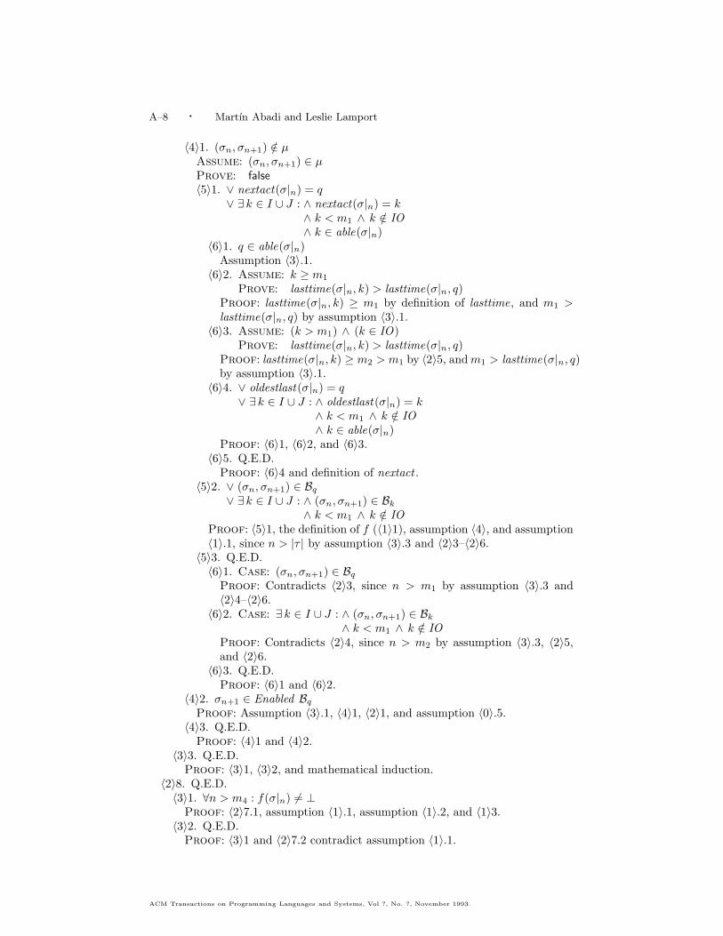
A–8 · Mart́ın Abadi and Leslie Lamport
〈4〉1. (σn, σn+1) /∈ µAssume: (σn, σn+1) ∈ µProve: false〈5〉1. ∨ nextact(σ|n) = q
∨ ∃ k ∈ I ∪ J : ∧ nextact(σ|n) = k∧ k < m1 ∧ k /∈ IO∧ k ∈ able(σ|n)
〈6〉1. q ∈ able(σ|n)Assumption 〈3〉.1.
〈6〉2. Assume: k ≥ m1
Prove: lasttime(σ|n, k) > lasttime(σ|n, q)Proof: lasttime(σ|n, k) ≥ m1 by definition of lasttime, and m1 >lasttime(σ|n, q) by assumption 〈3〉.1.
〈6〉3. Assume: (k > m1) ∧ (k ∈ IO)Prove: lasttime(σ|n, k) > lasttime(σ|n, q)
Proof: lasttime(σ|n, k) ≥ m2 > m1 by 〈2〉5, andm1 > lasttime(σ|n, q)by assumption 〈3〉.1.
〈6〉4. ∨ oldestlast(σ|n) = q∨ ∃ k ∈ I ∪ J : ∧ oldestlast(σ|n) = k
∧ k < m1 ∧ k /∈ IO∧ k ∈ able(σ|n)
Proof: 〈6〉1, 〈6〉2, and 〈6〉3.〈6〉5. Q.E.D.
Proof: 〈6〉4 and definition of nextact .〈5〉2. ∨ (σn, σn+1) ∈ Bq
∨ ∃ k ∈ I ∪ J : ∧ (σn, σn+1) ∈ Bk∧ k < m1 ∧ k /∈ IO
Proof: 〈5〉1, the definition of f (〈1〉1), assumption 〈4〉, and assumption〈1〉.1, since n > |τ | by assumption 〈3〉.3 and 〈2〉3–〈2〉6.
〈5〉3. Q.E.D.〈6〉1. Case: (σn, σn+1) ∈ Bq
Proof: Contradicts 〈2〉3, since n > m1 by assumption 〈3〉.3 and〈2〉4–〈2〉6.
〈6〉2. Case: ∃ k ∈ I ∪ J : ∧ (σn, σn+1) ∈ Bk∧ k < m1 ∧ k /∈ IO
Proof: Contradicts 〈2〉4, since n > m2 by assumption 〈3〉.3, 〈2〉5,and 〈2〉6.
〈6〉3. Q.E.D.Proof: 〈6〉1 and 〈6〉2.
〈4〉2. σn+1 ∈ Enabled BqProof: Assumption 〈3〉.1, 〈4〉1, 〈2〉1, and assumption 〈0〉.5.
〈4〉3. Q.E.D.Proof: 〈4〉1 and 〈4〉2.
〈3〉3. Q.E.D.Proof: 〈3〉1, 〈3〉2, and mathematical induction.
〈2〉8. Q.E.D.〈3〉1. ∀n > m4 : f(σ|n) �= ⊥
Proof: 〈2〉7.1, assumption 〈1〉.1, assumption 〈1〉.2, and 〈1〉3.〈3〉2. Q.E.D.
Proof: 〈3〉1 and 〈2〉7.2 contradict assumption 〈1〉.1.
ACM Transactions on Programming Languages and Systems, Vol ?, No. ?, November 1993.

An Old-Fashioned Recipe for Real Time · A–9
〈1〉5. Q.E.D.Proof: 〈1〉2, 〈1〉3, and 〈1〉4.
B6 Proof of Proposition 5
Assume: 1. Φ and Π are safety properties.2. (Φ −� Π, L1) is µ-machine realizable.3. (true, L2) is µ-machine realizable.4. Φ ∧Π ∧ L1 implies L2.
Prove: (Φ −� Π, L2) is µ-machine realizable.〈1〉1. Assume: ρ is a finite behavior such that ρ |= (Φ −� Π).
Prove: There exists a µ-strategy f such thatOµ(f, ρ) ⊆ (Φ −� Π) ∧ L2.
〈2〉1. Choose µ-strategy h such that Oµ(h, ρ) ⊆ (Φ −� Π) ∧ L1.Proof: Assumption 〈0〉.2, assumption 〈1〉, and Lemma 2.
〈2〉2. For all τ , choose a µ-strategy gτ such that Oµ(gτ , τ) ⊆ L2.Proof: Assumption 〈0〉.3 and Lemma 2.
〈2〉3. Let f(τ) = h(τ) for τ |= Φ, and otherwise let f(τ) = gη(τ) where η isthe shortest prefix of τ such that η �|= Φ. Then f is a µ-strategy.Proof: By steps 〈2〉1 and 〈2〉2 (which say that h and gη are µ-strategies).
〈2〉4. Oµ(f, ρ) ⊆ (Φ −� Π) ∧ L2
Assume: τ ∈ Oµ(f, ρ)Prove: τ ∈ (Φ −� Π) ∧ L2
〈3〉1. Case: τ ∈ Φ〈4〉1. τ ∈ Oµ(h, ρ)
Proof: By assumption 〈2〉, since the case assumption 〈3〉and the definition of f (step 〈2〉3) imply f(τ |n) = h(τ |n)for all n.
〈4〉2. τ ∈ (Φ −� Π) ∧ L1
Proof: By step 〈4〉1 and the choice of h (step 〈2〉1).〈4〉3. τ ∈ Φ ∧Π ∧ L1
Proof: By step 〈4〉2 and case assumption 〈3〉.〈4〉4. Q.E.D.
Proof: By step 〈4〉3 and assumption 〈0〉.4.〈3〉2. Case: τ �∈ Φ
〈4〉1. Let n be the least integer such that τ |n �∈ Φ.Proof: Such an n exists by case assumption 〈3〉 and as-sumption 〈0〉.1.
〈4〉2. τ ∈ Oµ(gτ |n , τ |n)Proof: By step 〈4〉1, assumption 〈2〉, and the definition off (step 〈2〉3).
〈4〉3. τ ∈ L2
Proof: By steps 〈4〉2 and the choice of gτ |n (step 〈2〉2).〈4〉4. Q.E.D.
Proof: By steps 〈4〉3 and case assumption 〈3〉.〈3〉3. Q.E.D.
Proof: By steps 〈3〉1 and 〈3〉2.〈2〉5. Q.E.D.
Proof: By steps 〈2〉3 and 〈2〉4.〈1〉2. Q.E.D.
Proof: The result follows immediately from step 〈1〉1 and Lemma 2.
ACM Transactions on Programming Languages and Systems, Vol ?, No. ?, November 1993.
A–10 · Mart́ın Abadi and Leslie Lamport
B7 Proof of Theorem 4
The proof of Theorem 4 is rather long and is presented in two steps. Section B7.1contains a high-level view of the proof; Section B7.2 contains the complete proof,omitting definitions and complete subproofs that appear in the high-level view. Ifa formula F is a conjunction, we may number the conjuncts and let F.i denote theith one.The proof uses the following two lemmas.Lemma Rule WF1. For any predicates P , Q, and I; actions N and A; and
state function f ; if(1) P ∧ I ∧ I ′ ∧ [N ]f ⇒ (P ′ ∨Q′)(2) P ∧ I ∧ I ′ ∧ 〈N ∧A〉f ⇒ Q′
(3) P ∧ I ⇒ Enabled 〈A〉f .then WFf (A) ∧ ✷I ∧ ✷[N ]f ⇒ (P ❀ Q)
Proof: This is a simple generalization of rule WF1 of [Lamport 1991]; the proofof soundness is omitted.
Lemma 4. For any actions A and B, state function f , variable x, predicate P ,and property Π:(1) (a) (Enabled (x′ = f)) = true.
(b) If A and B have no primed variables in common, then(Enabled A∧ B) = (Enabled A) ∧ (Enabled B).
(2) (Enabled A) ∧ (¬Enabled B) ⇒ (Enabled A∧ ¬B)(3) (Enabled P ∧A) = (P ∧ Enabled A)(4) (Enabled ∃x : A) = (∃x : Enabled A)(5) If A ⇒ B then (Enabled A)⇒ (Enabled B).Proof: These properties all follow easily from the definitions.
B7.1 High-Level Proof of the TheoremLet: Π ∆= E ∧M
M t ∆= M ∧ RT v ∧∀ i ∈ I : MinTime(ti,Ai, v) ∧ ∀ j ∈ J : MaxTime(Tj)
Πt ∆= E ∧M t
Assume: 0. a. Π = Init ∧ ✷[N ]w for some predicate Init , action N , and statefunction w.
b. ti is a timer for Π, for all i in I.c. Tj is a timer for Π, for all j in J .d. J is a finite set.
1. Πt ⇒ ✷(ti ≤ Tj), or 〈Ai〉v and 〈Aj〉v are disjoint for Π and i �= j, forall i ∈ I and j ∈ J .
2. a. now does not occur free in v.b. (now ′ = r) ∧ (v′ = v) is a subaction of Π, for all r ∈ R.
3. For all j ∈ J :a. 〈Aj〉v ∧ (now ′ = now) is a subaction of Π,b. Π ⇒ VTimer(Tj ,Aj ,∆j , v) or Π ⇒ PTimer (Tj ,Aj ,∆j , v), forsome ∆j ∈ ((0,∞)),
c. Πt ⇒ ✷(Enabled 〈Aj〉v = Enabled (〈Aj〉v ∧ (now ′ = now)))d. (v′ = v) ⇒ (Enabled 〈Aj〉v = (Enabled 〈Aj〉v)′)
4. E and M are safety properties, and M constrains at most µ.5. a. 〈Ak〉v ⇒ µ, for all k ∈ I ∪ J .
ACM Transactions on Programming Languages and Systems, Vol ?, No. ?, November 1993.

An Old-Fashioned Recipe for Real Time · A–11
b. (now ′ �= now)⇒ µProve: (E −� M t, NZ ) is µ-machine realizable.Proof sketch: We show that a fairness condition WF(now ,v)(C) implies that nowincreases without bound, for a subaction 〈C〉(now ,v) of Πt, and then apply Proposi-tions 4 and 5. To prove that now increases without bound, we prove that now = rleads to now ≥ (r + ∆) for any number r, where ∆ is the minimum of the ∆j .The action C advances now or, if that is impossible because now = Tj for someupper-bound timer Tj , it performs the action Aj (thereby advancing Tj).We begin by naming the next-state relations of the RT v, MaxTime, MinTime,VTimer , and PTimer formulas and defining some actions and predicates, includingC. A Bj step is defined to be an Aj step that leaves now unchanged. An At
j stepis an Aj step that satisfies the lower-bound timing constraint, if there is one. A Bt
j
step is a Bj step taken when Tj equals now that satisfies the lower-bound timingconstraint, if there is one. The state function T is the smallest Tj that restricts theadvance of now .Let: RTactv
∆= [(now ′ ∈ ((now ,∞))) ∧ (v′ = v)]now
MaxTact(t) ∆= [now ′ ≤ t′]now
MinTact(t,A, v) ∆= [A ⇒ (t ≤ now)]vVTact(t,A, δ, v) ∆= [∧ t′ = if (Enabled 〈A〉v)′
then if 〈A〉v ∨ ¬Enabled 〈A〉vthen now + δelse t
else ∞∧ v′ �= v](t,v)
PTact(t,A, δ, v) ∆= [∧ t′ = if Enabled 〈A〉vthen if 〈A〉v then now + δ
else telse t+ (now ′ − now)
∧ (now , v)′ �= (now , v)](t,v,now)
Pj∆= (j ∈ I)⇒ (tj ≤ now)
Atj
∆= Aj ∧ Pj
Bj ∆= Aj ∧ (now ′ = now)Btj
∆= Atj ∧ (now ′ = now) ∧ (Tj = now)
T∆= min{Tj : j ∈ J ∧ Enabled 〈Aj〉v}
∆ ∆= min{∆j : j ∈ J}NowT ∆= (now ′ = min(now +∆, T )) ∧ (v′ = v)C ∆= ∨ (T �= now) ∧ NowT
∨ (T = now) ∧ ∃ j ∈ J : Btj
〈1〉1. Choose JP and JV such that:1. J = JP ∪ JV2. JP ∩ JV = ∅3. ∀j ∈ JV : Π⇒ VTimer (Tj ,Aj ,∆j , v)4. ∀j ∈ JP : Π⇒ PT imer(Tj,Aj ,∆j , v)
Proof: JP and JV exist by assumption 〈0〉.3b.〈1〉2. Πt ⇒ ✷Inv , where
ACM Transactions on Programming Languages and Systems, Vol ?, No. ?, November 1993.

A–12 · Mart́ın Abadi and Leslie Lamport
Inv ∆= 1.∧ ∀j ∈ J : Tj ∈ [[now ,∞]]2.∧ now ∈ R3.∧ ∀j ∈ J : (Enabled 〈Aj〉v =
Enabled (〈Aj〉v ∧ (now ′ = now ))4.∧ ∀k ∈ I ∩ J : tk ≤ Tk5.∧ ∀j ∈ JV : ¬Enabled 〈Aj〉v ⇒ (Tj =∞)
Proof sketch: It follows immediately from the hypotheses that Πt implies✷Inv .3 and ✷Inv .4. The proofs for the other conjuncts of Inv are straightforwardbut somewhat tedious invariance proofs, which are omitted.〈2〉1. RT v ⇒ ✷Inv .2〈2〉2. For all j ∈ J : Π ∧ ✷Inv .2 ∧MaxTime(Tj)⇒ ✷Inv .1〈2〉3. Πt ⇒ ✷Inv .3〈2〉4. Πt ⇒ ✷Inv .4〈2〉5. Πt ⇒ ✷Inv .5〈2〉6. Q.E.D.
Proof: 〈2〉1–〈2〉5.〈1〉3. 1. Π = Init ∧ ✷M
2. Πt = Initt ∧ ✷N t, for some predicate Init t.whereM ∆= ∧ [N ]w
∧ ∀j ∈ JP : PTact(Tj ,Aj ,∆j , v)∧ ∀j ∈ JV : VTact(Tj,Aj ,∆j , v)
N t ∆= ∧M∧ RTactv∧ ∀i ∈ I : MinTact(ti,Ai, v)∧ ∀j ∈ J : MaxTact(Tj)
Proof: 1 follows from assumptions 〈0〉.0a and 〈0〉.3b, and 2 follows from thedefinition of Πt, since ✷ distributes over ∧. (A simple calculation shows thatM = [M]f and N t = [N t]g, for suitable tuples f and g, so ✷M and ✷N t areTLA formulas.)
〈1〉4. 〈C〉(now ,v) is a subaction of Πt.〈2〉1. For all j in J : 〈Bt
j〉v is a subaction of Πt.〈2〉2. 〈NowT 〉now is a subaction of Πt.〈2〉3. Q.E.D.
Proof: By 〈2〉1 and 〈2〉2, since 〈NowT 〉now = 〈NowT 〉(now ,v), 〈Btj〉v =
〈Btj〉(now ,v), Lemma 4.4 implies that the disjunction of subactions is a sub-
action, and Lemma 4.3 implies that if D is a subaction, then P ∧ D is also asubaction, for any predicate P .
〈1〉5. Πt ∧WF(now ,v)(C)⇒ NZProof: By the Lattice Rule [Lamport 1991], it suffices toAssume: r ∈ RProve: Πt ∧WF(now ,v)(C) ⇒ ( (now = r) ❀ (now ∈ [[r +∆,∞))) )Proof sketch: The standard method of proving that now = r leads to now ∈[[r+∆,∞)) is to assume that now = r and now is never in [[r+∆,∞)), and derivea contradiction. Step 〈2〉2 below proves that, if now equals r and it is never in[[r+∆,∞)), then it is always in [[r, r +∆)). It therefore suffices to assume now isalways in [[r, r +∆)) and derive the contradiction.The contradiction is obtained by showing that eventually there is no upper-boundtimer preventing the advance of now past r +∆. The timers that could prevent
ACM Transactions on Programming Languages and Systems, Vol ?, No. ?, November 1993.

An Old-Fashioned Recipe for Real Time · A–13
the advance of now are the ones in the set U of timers that are less than r +∆.Step 〈2〉4 asserts that U eventually becomes empty, and 〈2〉5 asserts that timethen advances past r +∆.Let: U ∆= {j ∈ J : Tj < r +∆}
V∆= {j ∈ J : now < Tj < r +∆}
TimerAct ∆= ∀j ∈ J : ∨ VTact(Tj ,Aj ,∆j , v)∨ PTact(Tj,Aj ,∆j , v)
〈2〉1. Inv ⇒ Enabled 〈C〉(now ,v)
〈2〉2. Πt ⇒✷((now = r) ∧ ✷(now ∈ ((−∞, r +∆))) ⇒ ✷(now ∈ [[r, r +∆))))
〈2〉3. Assume: j ∈ JProve: 1. Πt ∧ ✷(now ∈ [[r, r +∆))) ⇒ ✷((j /∈ U)⇒ ✷(j /∈ U))
2. Πt ∧ ✷(now ∈ [[r, r +∆))) ⇒ ✷((j /∈ V )⇒ ✷(j /∈ V ))〈2〉4. Πt ∧ ✷(now ∈ [[r, r +∆))) ∧WF(now ,v)(C) ⇒ ✸✷(U = ∅)〈2〉5. ∧ ✷(now ∈ [[r, r +∆)))
∧ ✷(U = ∅)∧ ✷Inv∧WF(now ,v)(C)⇒ true ❀ (now ≥ r +∆)
〈2〉6. Q.E.D.Proof: 〈2〉2, 〈2〉4, 〈2〉5, 〈1〉2, and temporal logic.
〈1〉6. (E −� M t, E ⇒WF(now ,v)(C)) is µ-machine realizable.〈2〉1. M t constrains at most µ.〈2〉2. Q.E.D.
Proof: We apply Proposition 4, with E substituted for Φ, M t substituted forΠ, and the single formula WF(now ,v)(C). Step 〈2〉1 asserts that M t constrainsat most µ. The three numbered hypotheses of the proposition are proved asfollows:1. 〈1〉4.2. Assumptions 〈0〉.5a and 〈0〉.5b and the definition of C.3. Vacuous.
〈1〉7. (true,NZ ) is µ-machine realizable.Proof: Assumption 〈0〉.5b.
〈1〉8. Q.E.D.Proof: Proposition 5, using 〈0〉.4, 〈1〉6, 〈1〉7, and 〈1〉5.
B7.2 Detailed Proof of the Theorem〈1〉1. Choose JP and JV such that:
1. J = JP ∪ JV2. JP ∩ JV = ∅3. ∀j ∈ JV : Π⇒ VTimer (Tj ,Aj ,∆j , v)4. ∀j ∈ JP : Π⇒ PT imer(Tj,Aj ,∆j , v)
〈1〉2. Πt ⇒ ✷Inv , whereInv ∆= 1.∧ ∀j ∈ J : Tj ∈ [[now ,∞]]
2.∧ now ∈ R3.∧ ∀j ∈ J : (Enabled 〈Aj〉v =
Enabled (〈Aj〉v ∧ (now ′ = now ))4.∧ ∀k ∈ I ∩ J : tk ≤ Tk5.∧ ∀j ∈ JV : ¬Enabled 〈Aj〉v ⇒ (Tj =∞)
ACM Transactions on Programming Languages and Systems, Vol ?, No. ?, November 1993.

A–14 · Mart́ın Abadi and Leslie Lamport
〈2〉1. RT v ⇒ ✷Inv .2Proof: An invariance proof.
〈2〉2. For all j ∈ J : Π ∧ ✷Inv .2 ∧MaxTime(Tj)⇒ ✷Inv .1Proof: Assumption 〈0〉.0c and an invariance proof.
〈2〉3. Πt ⇒ ✷Inv .3Proof: Assumption 〈0〉.3c.
〈2〉4. Πt ⇒ ✷Inv .4Proof: Assumption 〈0〉.1.
〈2〉5. Πt ⇒ ✷Inv .5Proof: 〈1〉1.3, assumption 〈0〉.3d, and an invariance proof.
〈2〉6. Q.E.D.〈1〉3. 1. Π = Init ∧ ✷M
2. Πt = Initt ∧ ✷N t, for some predicate Init t.whereM ∆= ∧ [N ]w
∧ ∀j ∈ JP : PTact(Tj ,Aj ,∆j , v)∧ ∀j ∈ JV : VTact(Tj,Aj ,∆j , v)
N t ∆= ∧M∧ RTactv∧ ∀i ∈ I : MinTact(ti,Ai, v)∧ ∀j ∈ J : MaxTact(Tj)
〈1〉4. 〈C〉(now ,v) is a subaction of Πt.〈2〉1. For all j in J : 〈Bt
j〉v is a subaction of Πt.Assume: j ∈ JProve: Πt ⇒ ✷ (Enabled 〈Bt
j〉v ⇒ Enabled (〈Btj〉v ∧ N t) )
〈3〉1. Πt ⇒ ✷ (Enabled (〈Btj〉v ∧M) ⇒
Enabled (∧ 〈Btj〉v ∧M
∧ ∀i ∈ I − {j} : ¬(〈Ai〉v ∧ 〈Aj〉v ∧M) ∨ (ti ≤ Tj) ) )〈4〉1. Πt ⇒ ¬Enabled (∃ i ∈ I − {j} : (〈Ai〉v ∧ 〈Aj〉v ∧M) ∧ ¬(ti ≤ Tj))
Proof: 〈1〉3.1, assumption 〈0〉.1, Lemma 4.3, and Lemma 4.4.〈4〉2. Q.E.D.
Proof: Lemma 4.2, substituting 〈Btj〉v ∧ M for A and ∃ i ∈ I − {j} :
(〈Ai〉v ∧ 〈Aj〉v ∧M) ∧ ¬(ti ≤ Tj) for B.〈3〉2. ∧ 〈Bt
j〉v ∧N t
∧ ∀i ∈ I − {j} : ¬(〈Ai〉v ∧ 〈Aj〉v ∧M) ∨ (ti ≤ Tj)= ∧ 〈Bt
j〉v ∧M∧ ∀i ∈ I − {j} : ¬(〈Ai〉v ∧ 〈Aj〉v ∧M) ∨ (ti ≤ Tj)
Proof: ∧ 〈Btj〉v ∧ N t
∧ ∀i ∈ I − {j} : ¬(〈Ai〉v ∧ 〈Aj〉v ∧M) ∨ (ti ≤ Tj)= [by definition of 〈Bt
j〉v]∧ At
j ∧ (v′ �= v) ∧ (now ′ = now) ∧ (Tj = now) ∧ N t
∧ ∀i ∈ I − {j} : ¬(〈Ai〉v ∧ 〈Aj〉v ∧M) ∨ (ti ≤ Tj)= [by definition of N t]∧ At
j ∧M∧ (v′ �= v) ∧ (now ′ = now) ∧ (Tj = now)∧ ∀i ∈ I : Ai ⇒ (ti ≤ now)∧ ∀i ∈ I − {j} : ¬(〈Ai〉v ∧ 〈Aj〉v ∧M) ∨ (ti ≤ Tj)
ACM Transactions on Programming Languages and Systems, Vol ?, No. ?, November 1993.

An Old-Fashioned Recipe for Real Time · A–15
= [by definition of Atj ]
∧ Pj ∧ Aj ∧M∧ (v′ �= v) ∧ (now ′ = now ) ∧ (Tj = now)∧ ∀i ∈ I : Ai ⇒ (ti ≤ now)∧ ∀i ∈ I − {j} : ¬(Ai ∧Aj ∧M∧ (v′ �= v)) ∨ (ti ≤ Tj)
= [by predicate logic]∧ Pj ∧ Aj ∧M∧ (v′ �= v) ∧ (now ′ = now ) ∧ (Tj = now)∧ (j ∈ I)⇒ (tj ≤ now)∧ ∀i ∈ I − {j} : ¬(Ai ∧Aj ∧M∧ (v′ �= v)) ∨ (ti ≤ Tj)
= [by definition of 〈Ak〉v]∧ Pj ∧ Aj ∧M∧ (v′ �= v) ∧ (now ′ = now ) ∧ (Tj = now)∧ (j ∈ I)⇒ (tj ≤ now)∧ ∀i ∈ I − {j} : ¬(〈Ai〉v ∧ 〈Aj〉v ∧M) ∨ (ti ≤ Tj)
= [by definition of Pj ]∧ Pj ∧ Aj ∧ (v′ �= v) ∧ (now ′ = now ) ∧ (Tj = now) ∧M∧ ∀i ∈ I − {j} : ¬(〈Ai〉v ∧ 〈Aj〉v ∧M) ∨ (ti ≤ Tj)
= [by definition of 〈Btj〉v]
∧ 〈Btj〉v ∧M
∧ ∀i ∈ I − {j} : ¬(〈Ai〉v ∧ 〈Aj〉v ∧M) ∨ (ti ≤ Tj)〈3〉3. Πt ⇒ ✷ (Enabled (〈Bt
j〉v ∧M)⇒ Enabled (〈Btj〉v ∧ N t) )
Proof: 〈3〉1, 〈3〉2, and Lemma 4.5.〈3〉4. Πt ⇒ ✷(Pj ∧ (Tj = now ) ∧ Enabled 〈Bj〉v ⇒ Pj ∧ (Tj = now) ∧
Enabled (〈Bj〉v ∧M))Proof: 〈1〉3, Assumption 〈0〉.3a, and the definition of Bj.
〈3〉5. Πt ⇒ ✷ ( (Enabled 〈Btj〉v)⇒ Enabled (〈Bt
j〉v ∧M) )Proof: 〈3〉4, the definition of Bt
j , and Lemma 4.3.〈3〉6. Q.E.D.
Proof: 〈3〉5 and 〈3〉3.〈2〉2. 〈NowT 〉now is a subaction of Πt.〈3〉1. Πt ⇒ ✷ ( (Enabled 〈NowT 〉now ) ⇒
(Enabled (〈NowT 〉now ∧M)) )〈4〉1. Πt ⇒ ✷ ( (Enabled NowT ) ⇒ (Enabled (NowT ∧M)) )
Proof: 〈1〉3, assumption 〈0〉.2b, and the definition of NowT , since Πt
implies Π.〈4〉2. Q.E.D.
Proof: 〈4〉1 and Lemma 4.3, substituting now �= T for P (since 〈NowT 〉now
equals NowT ∧ (now �= T )).〈3〉2. Πt ⇒ ✷(Enabled (〈NowT 〉now ∧M) ⇒
Enabled (〈NowT 〉now ∧ N t))〈4〉1. (Inv ∧ 〈NowT 〉now ∧M)⇒ (〈NowT 〉now ∧ N t)〈5〉1. Inv ∧ 〈NowT 〉now ⇒ RTactv
Proof: 〈1〉3 (Inv .1 and Inv .2).〈5〉2. ∀i ∈ I : 〈NowT 〉now ⇒ MinTact(ti,Ai, v)
Proof: MinTact(ti,Ai, v) = [ . . . ]v, and 〈NowT 〉now implies v′ = v.〈5〉3. ∀j ∈ J : Inv ∧ 〈NowT 〉now ∧M⇒ MaxTact(Tj)Assume: 1. j ∈ J
2. Inv ∧ 〈NowT 〉now ∧MProve: MaxTact(Tj)〈6〉1. Case: Enabled 〈Aj〉v〈7〉1. now ′ ≤ Tj
ACM Transactions on Programming Languages and Systems, Vol ?, No. ?, November 1993.

A–16 · Mart́ın Abadi and Leslie Lamport
Proof: Inv .1, Inv .2, 〈NowT 〉now , and the definitions of NowT ,since case assumption 〈6〉 and the definition of T imply Tj ≥ T .
〈7〉2. Case: j ∈ JP〈8〉1. Case: T ′
j = TjProof: 〈7〉1 and the definition of MaxTact(Tj).
〈8〉2. Case: T ′j = now +∆j
Proof: Inv .2, 〈NowT 〉now , and definition of MaxTact(Tj).〈8〉3. Q.E.D.
Proof: 〈8〉1, 〈8〉2, and case assumption 〈7〉, since case assump-tion 〈6〉 and the definition of PTact(Tj ,Aj ,∆j , v) imply thatthese are the only possibilities.
〈7〉3. Case: j ∈ JV〈8〉1. Tj = T ′
j
Proof: Case assumption 〈7〉 and the definitions of M andVTact(Tj ,Aj ,∆j , v), since 〈NowT 〉v implies v = v′.
〈8〉2. Q.E.D.Proof: 〈7〉1, 〈8〉1, and the definition of MaxTact(Tj).
〈7〉4. Q.E.D.Proof: 〈7〉2, 〈7〉3, 〈1〉1.1, and assumption 〈5〉.1.
〈6〉2. Case: ¬Enabled 〈Aj〉v〈7〉1. now ,now ′ ∈ R and now ′ > now .
Proof: Inv .1, Inv .2, 〈NowT 〉now , and the definition of T .〈7〉2. Case: j ∈ JP〈8〉1. T ′
j ≥ now ′
Proof: 〈7〉1, case assumption 〈7〉, Inv .1, and the definitions ofM and PTact(Tj ,Aj ,∆j , v).
〈8〉2. Q.E.D.Proof: 〈8〉1 and the definition of MaxTact(Tj).
〈7〉3. Case: j ∈ JV〈8〉1. Tj =∞
Proof: By case assumption 〈7〉 and Inv .5.〈8〉2. T ′
j =∞Proof: 〈8〉1, case assumption 〈7〉, and the definitions ofM andVTact(Tj ,Aj ,∆j , v), since 〈NowT 〉v implies v = v′.
〈8〉3. Q.E.D.Proof: 〈7〉1, 〈8〉2, and the definition of MaxTact(Tj).
〈7〉4. Q.E.D.Proof: 〈7〉2, 〈7〉3, 〈1〉1.1, and assumption 〈5〉.1.
〈6〉3. Q.E.D.Proof: 〈6〉1 and 〈6〉2.
〈5〉4. Q.E.D.Proof: 〈5〉1, 〈5〉2, 〈5〉3, and the definition of N t.
〈4〉2. Q.E.D.Proof: 〈4〉1 and 〈1〉2, since by Lemma 4.3 and Lemma 4.5, Inv ∧D ⇒ Eimplies ✷Inv ⇒ ✷((Enabled D)⇒ (Enabled E)), for any actions D and E .
〈3〉3. Q.E.D.Proof: 〈3〉1 and 〈3〉2.
〈2〉3. Q.E.D.〈1〉5. Πt ∧WF(now ,v)(C)⇒ NZ
Assume: r ∈ R
ACM Transactions on Programming Languages and Systems, Vol ?, No. ?, November 1993.

An Old-Fashioned Recipe for Real Time · A–17
Prove: Πt ∧WF(now ,v)(C) ⇒ ( (now = r) ❀ (now ∈ [[r +∆,∞))) )Let: U ∆= {j ∈ J : Tj < r +∆}
V∆= {j ∈ J : now < Tj < r +∆}
TimerAct ∆= ∀j ∈ J : ∨ VTact(Tj ,Aj ,∆j , v)∨ PTact(Tj,Aj ,∆j , v)
〈2〉1. Inv ⇒ Enabled 〈C〉(now ,v)
〈3〉1. Case: T �= nowProof: By the definition of C, since case assumption 〈3〉 impliesEnabled 〈NowT 〉now .
〈3〉2. Case: T = now〈4〉1. Choose j ∈ J such that (Tj = T ) ∧ Enabled 〈Aj〉v.
Proof: Inv .2, case assumption 〈3〉, and the definition of T .〈4〉2. (Tj = T ) ∧ Enabled 〈Bj〉v
Proof: 〈4〉1, Inv .3, and the definition of 〈Bj〉v.〈4〉3. Enabled 〈Bt
j〉vProof: 〈4〉2, Inv .4, case assumption 〈3〉, and the definition of 〈Bt
j〉v.〈4〉4. Q.E.D.
Proof: Case assumption 〈3〉, 〈4〉3, and the definition of C.〈3〉3. Q.E.D.
Proof: 〈3〉1 and 〈3〉2.〈2〉2. Πt ⇒
✷((now = r) ∧ ✷(now ∈ ((−∞, r +∆))) ⇒ ✷(now ∈ [[r, r +∆))))〈3〉1. ✷[RTactv]now ⇒ ((now = r)⇒ ✷(now ∈ [[r,∞))))
Proof: A standard invariance argument.〈3〉2. ✷[RTactv]now ⇒ ✷((now = r)⇒ ✷(now ∈ [[r,∞))))
Proof: 〈3〉1 and simple temporal logic.〈3〉3. Πt ⇒ ✷((now = r)⇒ ✷(r ≤ now ))
Proof: 〈3〉2, since Πt ⇒ RTv and RTv ⇒ ✷[RTactv]now .〈3〉4. Q.E.D.
Proof: 〈3〉3, using the temporal logic tautology(F ❀ G)⇒ ((F ∧ ✷H)❀ (G ∧ ✷H))
〈2〉3. Assume: j ∈ JProve: 1. Πt ∧ ✷(now ∈ [[r, r +∆))) ⇒ ✷((j /∈ U)⇒ ✷(j /∈ U))
2. Πt ∧ ✷(now ∈ [[r, r +∆))) ⇒ ✷((j /∈ V )⇒ ✷(j /∈ V ))Proof: A standard invariance proof, using assumption 〈0〉.3b.
〈2〉4. Πt ∧ ✷(now ∈ [[r, r +∆))) ∧WF(now ,v)(C) ⇒ ✸✷(U = ∅)Proof sketch: The set V consists of those timers in U that are not equalto now . To prove that U is eventually empty, we show that, whenever U isnonempty, eventually U or V gets smaller. Since U and V are finite, U musteventually become empty.〈3〉1. Assume: U0 and V0 sets, with U0 �= ∅.
Prove: ∧ ✷((U ⊆ U0) ∧ (V ⊆ V0))∧ ✷(now ∈ [[r, r +∆)))∧ ✷Inv∧ ✷[TimerAct ](now ,v)
∧WF(now ,v)(C)⇒ ((U = U0) ∧ (V = V0)) ❀
(U ⊂ U0) ∨ ((U ⊆ U0) ∧ (V ⊂ V0))
ACM Transactions on Programming Languages and Systems, Vol ?, No. ?, November 1993.

A–18 · Mart́ın Abadi and Leslie Lamport
Proof sketch: This is a straightforward application of rule WF1 (Lemma 3),with the following substitutions.Let: I ∆= 1.∧ now ∈ [[r, r +∆))
2.∧ (U ⊆ U0) ∧ (V ⊆ V0)3.∧ Inv
P∆= (U = U0) ∧ (V = V0)
Q∆= (U ⊂ U0) ∨ ((U ⊆ U0) ∧ (V ⊂ V0))
N ∆= TimerActA ∆= Cf
∆= (now , v)〈4〉1. I ′ ⇒ (P ′ ∨Q′)
Proof: Obvious.〈4〉2. Assume: P ∧ I ∧ I ′ ∧ 〈N ∧A〉f
Prove: Q′
〈5〉1. Case: T = now〈6〉1. Choose j in J such that (Tj = T ) ∧ 〈Bt
j〉v.Proof: A (from case assumption 〈4〉) and case assumption 〈5〉.
〈6〉2. T ′j ≥ r +∆
Proof: 〈6〉1, I.1, the definition of Btj, and TimerAct .
〈6〉3. j ∈ U ∧ j /∈ U ′
Proof: 〈6〉1, case assumption 〈5〉, and I.1.〈6〉4. j /∈ U ′
Proof: 〈6〉2.〈6〉5. Q.E.D.
Proof: 〈6〉3, 〈6〉4, and I ′.2.〈5〉2. Case: T �= now〈6〉1. (now ′ = T ) ∧ (v′ = v)
Proof: A and case assumption 〈5〉.〈6〉2. Case: T ∈ (now , r +∆)〈7〉1. Choose j in J such that (Tj = T ) ∧ Enabled 〈A〉v.
Proof: Case assumption 〈6〉 and the definition of T .〈7〉2. ∨ T ′
j = now ′
∨ T ′j ∈ [[r +∆,∞]]
Proof: 〈6〉1, 〈7〉1, I.1, and TimerAct .〈7〉3. j ∈ V
Proof: 〈7〉1, case assumption 〈6〉, and the definition of V .〈7〉4. j /∈ V ′
Proof: 〈7〉2 and the definition of V .〈7〉5. Q.E.D.〈7〉3, 〈7〉4, and I ′.2.
〈6〉3. Case: T ∈ [[r +∆,∞]]Proof: Impossible by 〈6〉1 and I ′.1.
〈6〉4. Q.E.D.Proof: 〈6〉2, 〈6〉3, I.3.1, and case assumption 〈5〉.
〈5〉3. Q.E.D.Proof: 〈5〉1 and 〈5〉2.
〈4〉3. P ∧ I ⇒ Enabled 〈A〉fProof: 〈2〉1.
〈4〉4. Q.E.D.
ACM Transactions on Programming Languages and Systems, Vol ?, No. ?, November 1993.

An Old-Fashioned Recipe for Real Time · A–19
Proof: 〈4〉1, 〈4〉2, 〈4〉3, and Lemma 3.〈3〉2. Assume: U0 and V0 sets, with U0 �= ∅.
Prove: Πt ∧✷(now ∈ [[r, r +∆))) ∧WF(now ,v)(C) ⇒((U = U0) ∧ (V = V0)) ❀
((U ⊂ U0) ∨ ((U ⊆ U0) ∧ (V ⊂ V0)))〈4〉1. Πt ⇒ ✷((U ⊆ U0) ∧ (V ⊆ V0)⇒ ✷((U ⊆ U0) ∧ (V ⊆ V0)))
Proof: Follows from 〈2〉3.〈4〉2. Q.E.D.
Proof: 〈3〉1, 〈4〉1, and 〈1〉2, since Πt ⇒ ✷[TimerAct ](now ,v) by assump-tion 〈0〉.3b.
〈3〉3. Q.E.D.Proof: Since U and V are finite by assumption 〈0〉.0d, it follows from〈3〉2 and the Lattice Rule [Lamport 1991] that Πt ∧ ✷(now ∈ [[r, r +∆))) ∧WF(now ,v)(C) implies ✸(U = ∅). By 〈2〉3, Πt ∧ ✷(now ∈ [[r, r +∆))) implies✸(U = ∅)⇒ ✸✷(U = ∅).
〈2〉5. ∧ ✷(now ∈ [[r, r +∆)))∧ ✷(U = ∅)∧ ✷Inv∧WF(now ,v)(C)⇒ true ❀ (now ≥ r +∆)
Let: I ∆= 1.∧ U = ∅2.∧ now ∈ [[r, r +∆))3.∧ Inv
P∆= true
Q∆= now ≥ r +∆
N ∆= true
A ∆= Cf
∆= (now , v)〈3〉1. I ∧ I ′ ∧ [N ]f ⇒ (P ′ ∨Q′)
Proof: Immediate, since P ′ = true.〈3〉2. Assume: P ∧ I ∧ I ′ ∧ 〈N ∧A〉f
Prove: Q′
〈4〉1. T ∈ [[r +∆,∞]]Proof: By I.
〈4〉2. 〈NowT 〉now
Proof: By 〈4〉1, I.2, and A.〈4〉3. Q.E.D.
Proof: 〈4〉1, 〈4〉2, and the definition of NowT .〈3〉3. P ∧ I ⇒ Enabled 〈A〉f
Proof: 〈3〉1.〈3〉4. Q.E.D.
Proof: 〈3〉1, 〈3〉2, 〈3〉3, and Lemma 3.〈2〉6. Q.E.D.
〈1〉6. (E −� M t, E ⇒WF(now ,v)(C)) is µ-machine realizable.〈2〉1. M t constrains at most µ.〈3〉1. M constrains at most µ.
Proof: Assumption 〈0〉.4.〈3〉2. RTv constrains at most µ.
Proof: Assumption 〈0〉.5b.
ACM Transactions on Programming Languages and Systems, Vol ?, No. ?, November 1993.

A–20 · Mart́ın Abadi and Leslie Lamport
〈3〉3. For all i in I, MinTime(ti,Ai, v) constrains at most µ.Proof: By definition of MinTime, a step violates MinTime(ti,Ai, v) onlyif it is an 〈Ai〉v step, so this follows from Assumption 〈0〉.5a.
〈3〉4. For all j in J , MaxTime(Tj) constrains at most µ.Proof: Assumption 〈0〉.5b.
〈3〉5. Q.E.D.Proof: 〈3〉1–〈3〉4 and the definition of M t.
〈2〉2. Q.E.D.〈1〉7. (true,NZ ) is µ-machine realizable.〈1〉8. Q.E.D.
ACM Transactions on Programming Languages and Systems, Vol ?, No. ?, November 1993.

Index
◦, 1546. . .′, 1548〈. . .〉..., 1548[. . .]..., 1548[[. . .]], 1548−�, 1563
action, 1548disjoint, 1550enabled, 1548subaction, 1550
agent, 1562assumption
environment, 1544, 1563granularity, 1559
assumption/guarantee specification, 1544,1563
and timing properties, 1567
behavior, 1549finite, 1549
Bernstein, Arthur, 1543Budhiraja, Navin, 1570
C(. . .), 1550canonical form, 1548, 1550closed set, 1549closed system, 1545closure, 1550completeness, 1550, 1557composition
and conjunction, 1564principle, 1565
constant, 1546constrains at most, 1562
and does not constrain, 1564and receptiveness, 1562and timing constraints, 1566
deadlock freedom, and nonZenoness,1559
∆=, 1546Dill, David L., 1562
Enabled, 1548environment, as part of system, 1545
fairness, 1548, 1549strong, 1548, 1549
weak, 1548, 1549feasibility, and machine closure, 1545finite internal nondeterminism (fin),
1551and history-determined variables,
1551and nonZenoness, 1559
Fischer, mutual exclusion protocol, 1560
guarantee, system, 1544, 1563
Harter, Paul K., Jr., 1543Head , 1546
implementation relation, 1545and implication, 1545for open systems, 1564
implication, intuitionistic, 1563initial state
and constrains at most, 1564in open systems, 1562
internal specification, 1547invariance, 1563
liveness, 1548and NZ , 1556in proof of safety, 1556
lower boundon action duration, 1544, 1559on time advance, 1559
machine closure, 1550and fairness, 1550and implication, 1551and nonZenoness, 1557and quantification, 1551
machine realizability, 1562and fairness, 1563and implication, 1563and machine closure, 1563and nonZenoness, 1568and quantification, 1563and receptiveness, 1563
Marzullo, Keith, 1570MaxTime, 1552MinTime, 1552
next-state relation, 1547calculation, 1564
A–21

A–22 · Mart́ın Abadi and Leslie Lamport
nonZenoness, 1557, 1568and δ-timers, 1559, 1568and quantification, 1559, 1569proving, 1559proving nonZenoness, 1568
now , 1543, 1552NZ , 1556
open system, 1544, 1562
paradoxcomposition, example, 1565Zeno’s, 1544
predicate, 1548type-correctness, 1547
property, 1549PTimer , 1553
quantificationover flexible variables, 1549over rigid variables, 1549
queuelossy, 1545real-time, 1553
receptiveness, 1562RT , 1552
safety, 1548, 1549and closed sets, 1549
Schneider, Fred B., 1560, 1570SF, 1549state, 1548
time-blocked, 1557state function, 1548step, 1548
stuttering, 1548stuttering, invariant under, 1549
Tail , 1546timer, 1552
lower-bound, 1552persistent δ-timer, 1553upper-bound, 1552volatile δ-timer, 1553
timing constraints, 1552in open systems, 1568
transition function, 1548
variableflexible, 1546
history, 1551history-determined, 1551internal, 1546, 1550rigid, 1546
VTimer , 1553
WF, 1549
Zeno, see also nonZenoness, 1557
ACM Transactions on Programming Languages and Systems, Vol ?, No. ?, November 1993.