An NPV Analysis of Buying versus Renting for Prospective

Australian First Home Buyers

Dominic Crowley∗ Shuyun May Li†

Abstract

This paper explores buying versus renting as an investment decision for a prospective Aus-

tralian first home buyer, by comparing the NPVs of buying and renting. An ex-post analysis

for overlapping 10-year periods from 1983 to 2013 for Australia’s eight capital cities suggests

that renting was favourable for the decade from 1983 in most capital cities and buying was

favourable from the early 1990s to early 2000s in all capital cities. An ex-ante analysis, using

different future scenarios for key variables identified in the ex-post analysis, suggests that in

2013 buying was favourable in Brisbane, Perth, Hobart and Darwin.

Keywords: NPV analysis; Australian housing market; Buying versus renting; First home buyer

JEL code: R30, E22, D14

∗Thanks for the generous support from my employer, the Productivity Commission, E-mail:

dpcrowley 3@hotmail.com.†Correspondence author, Department of Economics, The University of Melbourne, Tel: 61-3-83445316, E-mail:

shuyunl@unimelb.edu.au.

1

1 Introduction

Home ownership is an aspiration for most Australians and is deeply entrenched in Australian

culture, evident by cultural reference such as the ‘great Australian dream’ and ‘a man’s home is

his castle’. Home ownership provides security of tenure and the ability to renovate, and can have

financial benefits including increased wealth, a hedge against future rent increases and the ability to

leverage. Conversely, renting is often derided as an inferior choice with slogans such as ‘rent money

is dead money’ and ‘stop paying off someone else’s mortgage’. However, it is not clear whether

owning a house is superior to renting from a financial point of view. If a prospective buyer decides

to rent rather than buy she could invest the avoided one-off costs of buying, plus any difference in

ongoing costs, into other assets.

This paper explores buying versus renting by comparing the net present value (NPV) of buying

versus renting as an investment decision for a prospective first home buyer. An ex-post analysis

(was buying or renting favourable in the past) for past three decades and ex-ante analysis (is

buying or renting currently favourable) have been undertaken for each of Australia’s eight capital

cities, by considering various factors that are relevant for buying and renting decisions and using

data carefully collected from a number of sources. The ex-post analysis suggests that renting was

favourable for the decade from 1983 in most capital cities and buying was favourable from the early

1990s to 2000s in all capital cities. A sensitivity analysis shows that buying was more favourable

for long tenures and more risk averse investors. The ex-ante analysis suggests that in 2013 buying

was more favourable in Brisbane, Perth, Hobart and Darwin, whilst renting was more favourable

in Melbourne. We also conduct a switching analysis which illustrates that in most capital cities it

would have been favourable to switch between buying and renting at proper timing.

Our analysis closely follow the approach taken by Beracha and Johnson (2012) and Beracha,

Seiler and Johnson (2012) who present an NPV analysis of buying versus renting for overlapping

eight-year periods in the U.S. between 1978 and 2009. A number of studies have examined buying

versus renting in Australia by estimating the user cost of housing in Australia (Brown et al., 2011;

Fox and Tulip, 2014; Hill and Syed, 2012), in which the user cost of housing is typically measured

as the one-off costs and ongoing costs of buying less home price appreciation. Our study takes a

different approach to these previous studies as it directly estimates the NPVs of both buying and

renting for each of the eight capital cities.

2

There is also a broader literature on Australian housing market. Many studies have found

evidence of overvaluation in Australian housing market (Bodman and Crosby 2004; Fry, Martin

and Voukelatos 2010; Tumbarello and Wang 2010) while others suggest that home price growth can

be explained by economic fundamentals (Fox and Finlay 2012; Otto 2007). Some studies have found

overvaluation in Australian housing market in some periods and undervaluation in other periods

(Abelson et al. 2005; Fox and Tulip 2014; Hill and Syed, 2012). Whether housing is overvalued

is relevant to the buy versus rent decision. If housing is overvalued then renting is likely to be

financially optimal.

The rest of the paper proceeds as follows. Section 2 briefly describes some facts of Australian

housing market, which provide the background of this study. Section 3 describes the key assump-

tions in the analysis and how the NPVs of buying and renting are defined. Section 4 describes the

data sources and Section 5 presents the results. Section 6 concludes. Most tables and figures are

reported in the Appendix.

2 Background

The preference among Australians for buying over renting is longstanding. About 70 per cent of

Australians own their own home (ABS 2013). The home ownership rate has been about 70 per

cent for half a century, after increasing markedly (from less than 55 per cent) following World War

II (Eslake 2013).1 Various surveys show that most Australians aspire to be home owners.2

The preference for buying is likely due in part to real house price appreciation in recent decades

(Figure 1). Real house prices have increased more than threefold since 1983, much faster than

income growth. From 1983 to 2013, house prices increased markedly in each Australian capital

city, with median house prices increasing by at least two and a half times in real terms (average

1Home ownership also appears to be the preferred tenure type in many other developed countries. For example, inthe U.S., buying a home is often referred to as the ‘American dream’ (Beracha and Johnson 2012). Home ownershiprates are similar in other Anglophone countries. The home ownership rate was 67 per cent in the U.S. in 2007, 68 percent in Canada in 2006, and 67 per cent in New Zealand in 2006. However, home ownership rates vary dramaticallyacross other OECD countries. In 2006, the home ownership rate was much higher in Spain (90 per cent) and Italy(82 per cent) than Australia, but much lower in Germany (54 per cent) (ABS 2010).

2Baum and Wulff (2003) find that from the late 1970s to 1990 at least 40 per cent of non-home owning 25-34 yearolds expected to buy a home in the following five years, and most renters cited financial reasons for renting ratherthan buying. Merlo and McDonald (2002) find that in 1996-97, more than 50 per cent of those who did not own ahome or live with a homeowner viewed buying a home in the next three years as ‘important’ or ‘very important’ tothem. In a 2013 survey, 49 per cent of respondents who were intending to buy a home listed home ownership as thetop priority for their lifetime (Sweeney Research 2013).

3

annual growth rates of at least 3 per cent). Median house prices were the highest in Sydney at

both the beginning and end of this period. Growth was highest in Melbourne and Perth – in both

cities real prices increased by about three and a half times in real terms (average annual growth of

more than 4 per cent).

However, median house prices did not grow steadily over this period, hence the timing of buying

was critical to financial returns (Figure 2). In each capital city, there were prolonged periods where

the median house price rose strongly (for example, in Perth from 2002–07). In each city there were

at least four years where the median house price increased by more than 10 per cent in real terms.

On the other hand, there were also multi-year periods in each city where the median house price

was stable or fell slightly in real terms.

Growth in house prices has benefited existing home owners but it has made buying a home

more difficult, particularly for first home buyers. The overall home ownership rate has remained

fairly steady in recent decades but there has been a sharp decline in the home ownership rate for

younger people. From 1981–2011, the home ownership rate fell from 61 to 47 per cent among

households with a head aged 25–34 years and from 75 to 64 per cent for households with a head

aged 35–44 years (Eslake 2013). The ageing of the population has masked declines in age-specific

home ownership rates.

Prices for other asset classes have also increased in recent decades. The All Ordinaries Index

and house prices have increased by similar amounts in the past three decades (Figure 3), suggesting

that renters could have made large returns if they invested the avoided costs of buying in the share

market. And in recent decades, median rents have not grown as quickly as median house prices,

making renting more favourable.3

Could a financially disciplined person have chosen to rent rather than buy, invest additional

savings in shares or other assets and be better off financially?

3 The NPVs of Buying and Renting

We explore the buy versus rent decision by comparing the NPV of a prospective first home buyer

buying a median price house and selling T years later and that same person renting a house of

3Rental yields are estimated to have fallen from about 10 per cent to 5 per cent in most capital cities from1983–2003 and remained at about 5 per cent since 2003.

4

equivalent quality (same sale price) in the private rental market for T years. The NPV is the

discounted value of benefits less the discounted value of costs. If a prospective first home buyer

decides to rent rather than buy, they are assumed to invest the avoided one off costs of buying,

plus any difference in ongoing costs, into other assets. It is assumed that all costs in a particular

year are paid at the beginning of that year and all benefits are received at the end of that year.

Housing tenure choice is both a consumption and investment decision. Buying and renting

are both means for purchasing housing services. Consumption benefits from purchasing these

services, such as shelter, are not included in NPV analysis because these benefits are assumed to

be independent of tenure type (consistent with Fox and Tulip (2014)). These consumption benefits

are large, hence most our estimates of the NPV of buying and renting are negative.

3.1 Key Assumptions

The prospective buyer

We consider the buy versus rent decision for a prospective first home buyer. Buying a first home

is a very different decision to buying a second home. A second or subsequent home can be financed

from the sale of the first home or, if the first home is kept, it can be leveraged to finance the

purchase of additional homes. We consider owner occupiers rather than investors. The alternative

to buying a home is privately renting, as the prospective buyer is assumed to be ineligible for public

or social housing and not considering other tenure types.

The prospective buyer is assumed to invest the avoided one-off costs of buying, plus any dif-

ference in ongoing costs, into shares and/or term deposits if they choose to rent rather than buy.

She is assumed to have saved a deposit equivalent to 20 per cent of the median house price. This

assumption means that the prospective buyer will almost certainly be approved for a home loan

and avoid having to buy mortgage insurance. Besides, the prospective buyer is assumed to take

out a variable rate home loan, since only a relatively small proportion of home buyers take out

fixed rate loans – the proportion has fluctuated between about 5 and 20 per cent since the early

1990s (ABS 2014c). The loan balance is paid off when the property is sold. No assumptions are

made about the prospective buyer’s wealth, income, age, marital and parental status, gender, race

or education.

The property

5

The prospective buyer is assumed to buy or privately rent a median priced detached (separate)

and established house because most first home buyers buy these types of homes.4 This simplifies

the analysis as there are often body corporate fees for attached homes (such as apartments). There

are also various concessions for buying new homes that are not available for established homes. The

quality of the house is assumed to remain constant over the tenure length – the house is maintained

but there are no alterations or additions which improve its quality. However, to take depreciation

into consideration, we assume that the value of the house falls in value in subsequent years relative

to the median house price prevailing in each subsequent year.

Tenure length

In their study for the U.S., Beracha and Johnson (2012) assume a tenure length of eight years.

We consider a tenure length of ten years in the benchmark case, which appears to be a reasonable

assumption based on ABS data. Most first home buyers take out a home loan with a duration of

20, 25 or 30 years (ABS 2011). However, few first home buyers remain in their first homes for the

whole duration of the loans. The ABS (2009) find that in 2007-08, among home owners with a

mortgage (the category which most first home buyers are in): 42 per cent had moved in the past

five years; about 10 per cent had moved three or more times in the past five years; and the mean

number of moves in the past five years was 0.8.

If a prospective buyer decides to rent, they are assumed to move every three years. This

assumption also appears reasonable based on ABS data. In 2007-08, among renters in the private

rental market: 85 per cent had moved in the past five years; about 38 per cent had moved three or

more times in the past five years; and the mean number of moves in the past five years was 2.2.

Discount rate

We aim to make a ‘like-for-like’ comparison between buying and renting, so differences in risk

between buying and renting should be taken into consideration. However, it is unclear whether

owner occupied housing is more or less risky than investing in other assets (Fox and Tulip 2014).

Sinai and Souleles (2005) argue that home ownership provides a hedge against future rent risk,

as mortgage payments are based on a nominal loan amount and rents tend to rise with inflation.

On the other hand, mortgage interest rates can be volatile. In Australia they have tended to be

4During the past two decades, the proportion of first home buyers with a mortgage who lived in an establishedhome has fluctuated around 80 per cent. The proportion of first home buyers with a mortgage living in a detachedhouse has decreased in the past two decades but was still about 75 per cent in 2009-10 (ABS 2011).

6

more volatile than rent payments in recent decades. Homeowners are also exposed to the risk of

fluctuating house prices. Homeowners often have a large proportion of their wealth tied up in one

asset whereas renters can hold a more diversified portfolio (Di, Belsky and Liu 2007). Besides, risk

also depends on the specific type of house purchased, as well as other assets a prospective buyer

already holds. Both can vary greatly across prospective first home buyers.

Because the relative risk of owner occupied housing and renting is unclear, the same discount

rate is used for buying and renting in calculating the NPVs. The yields on 10-year Australian

government bond, which serve as risk free rates, are used to calculate the discount rates.

3.2 NPV of Buying

Next, we describe how the NPVs of buying and renting are defined. Table 1 gives a detailed

description of the variables and notations. All variables are nominal.

The NPV of buying and holding for T years is the discounted benefits of buying (discounted

net sale proceeds), less the discounted one-off costs, less the discounted ongoing costs:

NPV buy0 = benefitsbuy − costsoneoff buy − costsongoingbuy. (1)

All one-off costs are incurred at the start of the tenure. Hence they are not discounted. These

costs include a deposit, stamp duty, conveyancing, inspections, financing costs and other govern-

ment charges, less the first home owners grant and other concessions for first home buyers:

costsoneoff buy = deposit0 + duty0 + convey0 + inspect0 + fin0 + govt0 − FHOG0 − conc0 (2)

The ongoing costs of buying include mortgage repayments (loan amount times standard variable

rate), maintenance expenses, local government rates and building insurance. The ongoing costs are

discounted back to the start of the tenure using the discount rates for each year. Therefore:

costsongoingbuy = loan0 × SV R0 + maint0 + rates0 + buildins0

+T−1∑t=1

loant × SV Rt + maintt + ratest + buildinstΠt

u=1(1 + ru). (3)

The prospective buyer is assumed to have saved a 20 per cent deposit, and take out an interest

7

only loan, which means that the nominal balance of their loan remains the same throughout their

tenure. So in equations (2) and (3) above:

deposit0 = 0.2 ×medianprice0,

loan0 = 0.8 ×medianprice0,

loant = loan0, for t = 1, . . . T.

The net sale proceeds are the sale proceeds, less selling costs, less the outstanding loan balance.

Following Abelson and Chung (2004), a house bought at the median price is assumed to fall in

value in subsequent years relative to the median price by a factor of q each year. The net sale

proceeds are discounted for each year of the tenure. The benefits of buying are given by:

benefitsbuy =(1 − sc) ×medianpriceT × (1 − q)T − loanT

ΠTt=1(1 + rt)

(4)

3.3 NPV of Renting

The NPV of renting for T years is the discounted net benefits of renting (from investing into other

assets), less the discounted one-off costs of renting, less the discounted ongoing costs of renting:

NPV rent0 = benefitsrent − costsoneoff rent − costsongoingrent. (5)

The only one-off cost of renting is a rental bond equivalent to 10 per cent of the annual rent:

costsoneoff rent = 0.1 × rent0 = bond0 (6)

The ongoing costs of renting consist of rent payments and additional moving costs, since renters are

assumed to move every three years. Ongoing costs are discounted back to the start of the tenure

using discount rates for each year:

costsongoingrent = rent0 +T−1∑t=1

renttΠt

u=1(1 + ru)+

∑m=3,6,9

movingcostsmΠm

u=1(1 + ru)(7)

A renter is assumed to sell her investment portfolio after T years. The net benefits of renting

8

comprise of the sale yield of the renter’s investment portfolio at the end of year T, plus dividends

on shares, less capital gains tax (CGT) paid on sale yield of shares, less the initial investment:

benefitsrent =s× ΠT

t=1(1 + rsht ) + (1 − s) × ΠTt=1

(1 + rtdt (1 − tinc)

)ΠT

t=1(1 + rt)× invest0

+

T∑t=1

(1 − tinc) × dividendtΠt

u=1(1 + ru)− CGTT

ΠTt=1(1 + rt)

− [costsoneoff buy − costsoneoff rent] (8)

A more detailed explanation of Eq. (8) follows. A renter is assumed to invest in shares and

term deposits, in proportions s and 1 − s, respectively. Post-tax returns on term deposits are

used. Brokerage and other costs incurred in establishing an investment portfolio are assumed to be

negligible. The amount invested in other assets comprises an initial investment and investment of

the differences between the ongoing costs of buying and renting. To simplify analysis, differences

between these ongoing costs in all subsequent years are discounted back to the start of the tenure.

As a result, total investment in other assets, in present value term, is given by:

invest0 = costsoneoff buy − costsoneoff rent + costsongoingbuy0 − costsongoingrent0

+

T−1∑t=1

costsongoingbuyt − costsongoingrentt

Πtu=1(1 + ru)

Total investment timing the average return on the investment portfolio gives the sale yield of the

renter’s investment in other assets.

Dividends on shares in a particular year are calculated as the product of dividend yield and

the average of the initial and final nominal values of the shares. Tax is paid at an individual’s

marginal tax rate (assumed to be 40 per cent). Dividends are assumed to be consumed rather than

reinvested. So the after-tax dividends on shares received in a particular year are given by:

dividendt = (1 − tinc) × dyieldt ×[0.5 × s× [invest0 + invest0 × ΠT

t=1(1 + rsht )]]

In September 1985, CGT was introduced for shares (and other assets) purchased after this date.

CGT was payable at an individual’s marginal tax rate on the ‘indexed’ capital gain (adjusted for

inflation) when shares were sold. In September 1999, indexation was replaced with a ‘discount’

method, where CGT was payable on only half of the capital gain for shares purchased after this

9

date (ATO 2014). So the CGT paid on sale yield of shares at the end of period T is given by:

CGTT = s×[invest0 × ΠT

t=1(1 + rsht ) − invest0

]× CPIT

CPI0× tinc, for shares purchased from 1986–99

CGTT = 0.5 × s×[invest0 × ΠT

t=1(1 + rsht ) − invest0

]× tinc, for shares purchased from 2000

Table 1: Variables in the NPV analysis

Variable notation Variable description

bond0 Rental bond, equivalent to 10 per cent of annual rent (When a renter moves theyare assumed to fund the bond on her new property with the bond refunded fromher previous property)

buildinst Building insurance in a particular yearCGTT Capital gains tax paid on sale yields of shares at the end of the tenure lengthconc0 Concessions for first home buyers such as stamp duty concessionsconvey0 Conveyancing feesCPIt Consumer Price Indexdeposit0 Mortgage deposit, assumed to be 20 per cent of purchase pricedividendt Dividend on shares received in a particular yearrt risk free rate in a year, the Australian Government 10 year bond rate is usedduty0 Stamp duty paid on the median priced housedyieldt Fully franked dividend yield in a year. Historical estimates were collected.FHOG0 First Home Owners Grantfin0 Financing costs associated with taking out a mortgagegovt0 Government charges other than stamp duty such as mortgage registration feesinspect0 Inspection costs, including building and pest inspectionsinvest0 Total investment by a renter into other assets, including initial investment and

the difference in the ongoing costs of buying and rentingloant Loan balance in a particular yearbond0 Annual maintenance expenses in a particular yearmedianpricet Median house price in a particular yearmovingcostsm Moving costs in a particular yearNPVbuy The net present value of buying at the start of the tenure lengthNPVrent The net present value of renting at the start of the tenure lengthq A house purchased at the median price is assumed to decrease in value by q per

cent relative to the median price for each year it is heldratest Local government rates in a particular yearrentt Rent payable in a particular yearrsht Return on shares in a particular yearrtdt Return on term deposits in a particular years Proportion of total investment a renter invests in sharessc The costs of selling a house, such as agent fees, assumed to be 3 per cent of sale

priceSV Rt Standard variable rate on mortgage in yeartinc Marginal income tax rate, a constant marginal tax rate of 40 per cent is assumed

10

4 Data

A number of data sources are used to collect data for the variables in the NPV analysis.5

4.1 Median House Prices

Many private companies such as Australian Property Monitors, BIS Shrapnel, the Real Estate

Institute of Australia (REIA), Rp Data and Residex, have estimates of current and historical house

prices. These data are prohibitively expensive for us to obtain. Instead, estimates of median

house prices for Australia’s eight capital cities from 1983–2003 have been sourced from Abelson

and Chung (2004) in which they investigate a number of different data sources and choose their

preferred estimates for each year and city. These estimates have been spliced with the REIA

estimates for 2004-2013 to create the median house prices data for our analysis.6

There is no agreed method on how to measure house prices in Australia. Australian houses

are bought and sold irregularly. Prasad and Richards (2006) estimate that about 6 per cent of

the housing stock in Australia are transacted each year. Changes in median prices result from

changes in the composition of properties sold, changes in the quality of housing and ‘pure’ house

price change. Median prices are also affected by measurement and data quality issues, and lags

between when a transaction is settled and when it is recorded. Simple median house price measures

have been found to be much more volatile than measures that adjust for these biases. Techniques

to adjust for these biases include: repeat sales measures, which compare sale prices of the same

houses over time; mix-adjusted or stratified measures, which weigh different groups of properties;

and hedonic or regression based measures, which adjust for the characteristics of properties. These

more sophisticated measures have been applied in Hansen (2006) and Prasad and Richards (2006)

to produce house price estimates.

The median house prices estimates used in our analysis have also been smoothed. The annual

estimates for 1983-2003 are from Abelson and Chung (2004), which have been smoothed by av-

eraging quarterly estimates (from REIA data for most capital cities and other data sources for

the rest). The annual estimates for 2004-2013 are obtained by averaging quarterly estimates from

5The source data can be made available upon readers’ request.6The REIA house price data for 2004-2013 are available at the research resource of the Faculty of Business and

Economics, University of Melbourne. For more recent years, median house price estimates by most of the privatecompanies mentioned above can be found through web searching. These estimates are broadly consistent with theseries we use in the analysis.

11

REIA. Averaging quarterly estimates significantly reduces the volatility of the median house price

series. For this reason, further smoothing techniques are not applied.

4.2 Benefits of Buying

The benefit of buying in this analysis comes from selling the house at the end of the tenure length.

A house is assumed to be bought at the median price. However, the house is assumed to sell for

1 percent less than the median price for each year that the property is held. This assumption is

based on Abelson and Chung (2004) who argue that the quality of the housing stock have increased

over time by about 1 per cent per year on average. Selling costs in 2013 are estimated to account

for about 3 per cent of the sale price in each capital city based on web searching. This estimate is

consistent with Fox and Tulip (2014). We assume that selling costs account for 3 per cent of the

sale price in all capital cities and for the whole study period.

As discussed above, people might obtain utility from being a home owner. There might be non-

financial psychic benefits, such as freedom to renovate and security of tenure. These issues have

been topical in recent years, as renting has become more common, particularly among families

(Tenants Union of Victoria 2014). These benefits of buying are not considered in this analysis.

4.3 Costs of Buying

One-off costs of buying

Costs of buying includes one-off costs and ongoing costs. The key one-off costs of buying a home

are a deposit and stamp duty. The prospective buyer is assumed to have saved a deposit equal

to 20 per cent of the purchase price. In Australia, stamp duties are levied by state and territory

governments on the transfer of property, including residential property. Stamp duties are typically

progressive taxes where higher rates apply to higher price properties. Thresholds have increased

over time. We have collected stamp duty regimes from various sources for each state and territory.7

Some states and territories have, or have had, stamp duty concessions for first home buyers. These

are taken into account in the analysis where possible. Stamp duty rates for each state and territory

are applied to median house prices to estimate how much a propective first home buyer would have

paid in stamp duty in a particular year and city.

7Current rates are freely available on the Internet. Historical information is more difficult to find and has beenfound through contacting state revenue offices and treasuries and searching through historical versions of legislations.

12

Other one-off costs are first estimated for 2013 based on web searching. First, conveyancing fee

(and other legal costs) is assumed to cost AUD1500 in each city. Second, financing costs such as

valuation fees and establishment fees are assumed to total AUD500 in each city (ASIC 2014; NSW

Family and Community Services 2014). Third, inspections are assumed to cost AUD800 in each

city, based on cost ranges found for building and pest inspections (NSW Family and Community

Services 2014). These inspections are assumed to be purchased by 50 per cent of buyers. Hence an

estimate of AUD400 is used as the inspection cost. Fourth, government mortgage registration and

transfer fees in 2013 are obtained for each city based on web searching.

For one-off costs in previous years, historical data have been used, where possible. But in most

cases, historical estimates are not available. So these one-off costs are assumed to have grown with

the city-specific CPI during the study period; the furnishings, household equipment and services

CPI is used. First home owner grants (FHOG) partially offset one-off costs. Historical information

on FHOG schemes has been collected to construct the estimates for each state and territory.

Ongoing costs of buying

Mortgage repayments are the key ongoing cost of buying. As the prospective first home buyer

is assumed to take out an interest-only variable rate loan, the mortgage repayment for a particular

year is simply the product of the average standard variable rate in that year and the loan balance.

Other ongoing costs considered are local government rates, maintenance and building insurance.

Local government rates for 2013 are collected for capital cities where there is only one local govern-

ment body (Brisbane, Canberra, Hobart and Darwin). Average rates across major local government

bodies are used for other capital cities. Historical data are collected from local governments, where

possible. Fox and Tulip (2014) estimate that landlords spend 6.3 per cent of gross annual rental

income on repairs and maintenance, based on data from the Australian Taxation Office. We use

a slightly higher value for annual maintenance costs – 7.5 per cent of annual rent, because owner

occupiers tend to spend more than landlords on maintenance. Building insurance is assumed to

increase with house prices, and cost AUD 200 annually per AUD 100 000 insured in 2013. Where

historical estimates are not available, costs are assumed to have grown with the city-specific CPI.

Contents insurance is not considered because it can be bought by both home owners and renters.

13

4.4 Benefits of Renting

If the prospective first home buyer decides to rent rather than buy, they are assumed to invest the

avoided costs of buying into a mix of higher risk and lower risk assets (shares and term deposits).

The portfolio of shares is assumed to follow the All Ordinaries Index and is sold at the end of the

tenure length. The appropriate CGT regime has been applied – there have been three different

regimes during the study period as described earlier. The marginal income tax rate is assumed to

be 40 per cent. Dividend yield estimates are collected for each year from 1983-2013.

Historical returns on term deposit have been sourced from the Reserve Bank of Australia.

The prospective buyer is assumed to invest in annual term deposits (longer term returns are only

negligibly higher) and reinvest the principal and all post-tax earnings into annual term deposits.

4.5 Costs of Renting

Costs of renting include one-off costs and ongoing costs. A bond equivalent to ten per cent of

annual rent (about five weeks’ rent) is the only one-off cost of renting. The bond is returned when

the renter moves and used to pay the bond on the next property she rents.

Rent payments are the main ongoing costs of renting. We aim to compare buying a median price

house and renting a house of equivalent quality, however, rent payable on the median price house

in a city is not necessarily equal to the median rent since the composition of the owner-occupied

and rental housing stock differ.8 Hence, we use rental yields – annual rent relative to the price of

a house – to estimate rent paid on the median price house. Rental yields for 2013 for each capital

city are publicly available from a number of private data providers. Rp Data yields for the second

quarter of 2013 are used because Rp Data ‘matches’ rented and sold properties (Fox and Tulip

2014). The rental yields are then applied to the median house prices to estimate rents payable in

2013. Historical data on rental yields are unavailable.9 So REIA data on median rents and median

house prices for three bedroom houses are used to construct the historical estimates of rental yields.

The other ongoing cost of renting is moving cost. The prospective buyer is assumed tol move

every three years if she chooses to rent. Based on web searching, direct moving costs in 2013 are

estimated to be AUD 2,000. Moving costs are assumed to be the same across cities. Historical

8Hill and Syed (2012), using a dataset of 900, 000 price and rent observations for Sydney in 2001-2009, find thatthe price of the median sold dwelling was 18 per cent higher than the imputed price of the median rented dwelling.

9A number of private organisations may have current and historical estimates of rental yields for Australian capitalcities, however, purchasing these data is prohibitively expensive.

14

estimates are not available so moving costs are assumed to have grown with the city-specific CPI.

Many renters pay ‘double rent’ around the time that they move – rent on both their existing

property and the property they are about to move into. So we assume that the prospective buyer

pays one month of double rent each time she moves. Other costs, such as time and money spent

searching for a house, are not considered.

5 Results

5.1 Ex-post NPV Analysis

Benchmark case

The benchmark case in the ex-post analysis considers a prospective first home buyer deciding

whether to buy a median price house and hold it for 10 years or rent a house of equivalent quality

for 10 years and invest avoided one-off costs of buying, plus any difference in ongoing costs, equally

between shares and term deposits. Sensitivity analysis is undertaken on the tenure length and

investment portfolio of the prospective buyer. All other assumptions discussed in Section 3 and 4

are applied in both the benchmark case and sensitivity analysis.10

Table 2 outlines the ex-post analysis results for the benchmark case. Between 1983 and 2013

there are 21 overlapping 10-year periods, the first period beginning in 1983 and the final period

beginning in 2003. Table 2 reports, for each 10-year period and each capital city, whether ‘Buy’

or ’Rent’ was more favorable financially.11 The results suggest that timing had a critical effect

on the relative financial returns of buying and renting in Australian capital cities from 1983–

2003. Renting was financially optimal (renting had a higher NPV than buying) in most Australian

capital cities and in most years from 1983–1992. However, for all Australian capital city, buying was

financially optimal in almost all years from 1993–2003. Patterns show some similarity across capital

cities, however, there are city-specific differences. From 1983–2003, buying was most favourable in

Brisbane (for 17 of the 21 years) and Sydney (15 out of 21 years) and least favourable in Perth and

10A ‘Buy versus Rent’ model has been built in Excel to undertake the ex-post and ex-ante NPV analysis. Ithas been used to compute the NPV of buying and the NPV of renting. It also contains sub-models to calculate therequired rate of appreciation to equalise the NPV of buying and renting, determine whether switching between tenuretypes is optimal, calcualte the user cost of buying, and examine the sensitivity of results to different tenure lengths,investment portfolios and discount rates. The model is flexible – results can be regenerated easily and data can beupdated. The model is available from the authors upon request.

11Results are not reported for Hobart, 1983–86, and Darwin, 1983–1993, because the ex-post analysis is notundertaken due to unavailability of median rental estimates.

15

Canberra (for 9 of 21 years).

Table 2: Buy or rent, Australian capital cities, 1983-2003 (Benchmark case)

Buy year Sydney Melbourne Brisbane Adelaide Perth Hobart Darwin Canberra

1983 Buy Buy Buy Buy Rent ne ne Rent1984 Buy Rent Buy Rent Rent ne ne Rent1985 Buy Rent Buy Rent Rent ne ne Rent1986 Buy Rent Buy Rent Rent ne ne Rent1987 Buy Rent Buy Rent Rent Rent ne Rent1988 Rent Rent Buy Rent Rent Rent ne Rent1989 Rent Rent Rent Rent Rent Rent ne Rent1990 Rent Rent Rent Rent Rent Rent ne Rent1991 Rent Rent Rent Rent Rent Rent ne Rent1992 Buy Buy Rent Rent Rent Rent ne Rent1993 Buy Buy Buy Buy Rent Buy ne Rent1994 Buy Buy Buy Buy Rent Buy Buy Buy1995 Buy Buy Buy Buy Buy Buy Buy Buy1996 Buy Buy Buy Buy Buy Buy Buy Buy1997 Buy Buy Buy Buy Buy Buy Buy Buy1998 Buy Buy Buy Buy Buy Buy Buy Buy1999 Buy Buy Buy Buy Buy Buy Buy Buy2000 Buy Buy Buy Buy Buy Buy Buy Buy2001 Buy Rent Buy Buy Buy Buy Buy Buy2002 Rent Rent Buy Buy Buy Buy Buy Buy2003 Rent Rent Buy Buy Buy Buy Buy Rent

In most years and for most capital cities one tenure type tended to be clearly favourable to the

other – the difference between the NPVs of buying and renting was more than AUD10,000, see

Table 4 in the Appendix. This table reports the estimated values for the NPVs of buying, NPVs

of renting and the difference between the NPVs of buying and renting. As consumption benefits

of housing are not considered, the NPV estimates tend to be negative. The NPVs of buying were

more volatile than the NPVs of renting, driven by the uneven rates of house price appreciation in

each capital city from 1983–2013 (see Figure 2 in the Appendix).12

Required rates of appreciation

Another method to investigate whether buying or renting is more favourable is to calculate the

required rate of house price appreciation over a tenure length that equalises the NPVs of buying

and renting, and compare it to the actual rate of house price appreciation over that tenure length.

If the required rate is higher (lower) than the actual rate, renting (buying) is more favourable.

12Standard errors of the NPV of buying and renting have not been estimated because standard errors for mostsource data are unavailable.

16

For tenures beginning between 1983 and the early 1990s, the required real rates of appreciation

over a ten year tenure tend to be higher than the actual real rates of appreciation (see Figure 4 in

the Appendix), especially for Adelaide and Canberra, suggesting that renting was more favourable.

The required rates fall across capital cities from the early 1990s, driven by falling mortgage rates,

and then fall further from the late 1990s due to the collapse of the share market following the GFC

– the All Ordinaries Index fell by more than 40 per cent in 2008. In particular, the required rates

are very low in the late 1990s because house prices appreciated rapidly in the following decade,

suggesting that buying was much more favourable in the late 1990s. In fact, from the early 1990s to

2003, the actual rates of appreciation were much higher than the required rates in most cities. By

the late 1990s, the difference between the actual and required rate were more than five percentage

points in all capital cities apart from Sydney and Melbourne.

Sensitivity analysis

Sensitivity analysis is undertaken on tenure length and the renter’s investment portfolio because

there is large variation in tenure length and risk preferences. Sensitivity analysis for the discount

rates has also been undertaken, whereby the annual risk free rate is increased by 1–5 percentage

points, but results do not change much so this is not discussed further. In the sensitivity analysis,

the NPVs of buying and rentingl are calculated for each capital city, with tenure lengths from one

to 20 years (at one year intervals) and three different investment portfolios: 100 per cent in shares

and 0 per cent in term deposits; 50 per cent in shares and 50 per cent in term deposits; and 0 per

cent in shares and 100 per cent in term deposits.13

From 1983–2013, in all capital cities, buying tended to be more favourable as tenure length

increased, and renting was more favourable than buying in most years for shorter tenure lengths

(less than five years), see Figure 5 in the Appendix. This was particularly the case for more risk

averse people–they would have invested in term deposits rather than shares if choosing to rent

rather than buy as term deposits are typically less risky and have lower returns than shares.

Sydney and Brisbane appear to have been the most favourable cities for buying. Buying was

particularly favourable in Brisbane for more risk averse investors who had longer tenure lengths.

Canberra and Perth were the most favourable cities for renting because rental yields were relatively

13This analysis is limited by the data, as fewer longer tenure lenghts can be considered than shorter tenure lengths.For example, using our data from 1983–2013, 30 one-year tenures, 29 two-year tenures, and only 11 tenure lengths of20 years can be analysed. Besides, for Hobart and Darwin, data are unavailable for some years.

17

low in both cities. The result for Perth is surprising given its high house price appreciation relative

to other cities. However, house price appreciation has been uneven in Perth, which drives this

result. For example, appreciation was very high from 2002–07 but has been flat since. In some

capital cities, the proportion of years where buying was favourable was very different for more risk

averse people and less risk averse people, particularly for longer tenure lengths.

Comparison of results with other literature

As discussed in the Introduction, existing Australian studies on buying versus renting have

focused on estimating the user cost of buying a home. For instance, Brown et al. (2011) estimate

the user cost of buying a home and holding it for five years in Sydney, Melbourne and Brisbane

from 1988–2004. To compare our results with theirs, we have transformed our results from the

ex-post analysis into user costs of buying, where the user costs are calculated as the negative of the

NPVs of buying and holding for five years divided by five years and then divided by the purchase

price. Both sets of results are similar for most years across the three cities, and there are similar

patterns over time (see Figure 6 in the Appendix).

Fox and Tulip (2014) estimate the user cost of buying for Australia, rather than for specific cities,

from the early 1980s to 2014 using a constant real expected appreciation rate equal to the 1955–

2014 average. They find that the user cost of housing fluctuated around 8 per cent from the early

1980s to early 1990s, then fell steadily to about 4 per cent by 2005, and then fluctuated between

4 and 5 per cent from 2005–2014. Even though their estimates are much less volatile than those

displayed in Figure 6, as a result of using a constant rate of appreciation, their results also show

declining user costs through the 1990s. Fox and Tulip (2014) also assess whether housing was under

or overvalued during this period, using a 10-year rolling appreciation rate. Their finding suggest

that buying appeared to be favourable in the mid-1980s and renting appeared to be favourable for

most of the 1990s, which is in contrast to our results from the ex-post analysis. Hill and Syed (2012)

find that the price-rent ratio was above equilibrium in Sydney from 2001–2008, favouring renting,

but by 2009 the price-rent ratio was at about equilibrium level. This is in line with our results that

renting was favourable in Sydney from 2002–09 although buying was favourable in 2001.

Switching analysis

The ex-post analysis suggests that it was financially optimal to buy in some years and rent

in other years during the past three decades. However, this analysis does not assess whether it

18

might have been optimal to switch between tenure types (buying and renting). We consider six

20-year periods. The first period begins in 1983, the sixth or final period begins in 1993 and other

periods are spaced two years apart. And we explore for each 20-year period whether buying for the

whole period, renting for the whole period, or switching tenure type once in a certain year would

have been optimal. Switching is considered at four year intervals during each 20-year period. All

Australian capital cities are considered apart from Darwin, for which data are unavailable.

From 1983–2013, for selected 20-year periods, switching between tenure types was favourable in

most capital cities since switching had a higher NPV than buying (only) or renting (only) for the

whole period (see Table 5 in the Appendix). Renting and then buying tended to be more favourable

than buying and then renting, consistent with the ex-post analysis which find that renting was

favourable in most capital cities from 1983 to the early 1990s and buying was favourable from the

early 1990s. Even though the financially optimal option varied across capital cities for some 20-year

periods, there were no cases where renting for the full 20-year period was optimal.

5.2 Ex-ante NPV Analysis

We have focused on an ex-post analysis of buying versus renting. However, in reality, buying a home

is an ex-ante decision. A prospective first home buyer has expectations about the costs and benefits

of buying a home but does not know these costs and benefits with certainty. Expectations vary

across people – some people might be more optimistic about house price appreciation. Modelling

expectations is beyond the scope of the paper. Next, we conduct an ex-ante analysis which considers

various hypothetical future scenarios from 2013 and explores for each scenario whether buying or

renting is favourable in 2013.

Again we consider the benchmark case in the ex-post analysis; a prospective first home buyer

either buys an established, detached and median priced house and lives in it for 10 years or rents

an established and detached house of equivalent quality for 10 years (but moves every three years).

Four key variables are considered to construct future scenarios. First, future (10 year) share market

return is considered to take one of the following 3 values: average real growth rate of share prices

over 1983-2013 (4.2 per cent per annum); average real growth rate over 2004-2013 (2.1 per cent

per annum); or a real growth rate of 3 per cent per annum. Second, future real mortgage rate is

considered to be: the average mortgage rate over 1983–2013 (5.7 per cent); the average mortgage

19

rate over 2004-2013 (4.4 per cent); or 5 per cent. Third, future real house price growth in each

city is considered to be: the 1983-2013 city-specific averages; the 2003-2013 city-specific average;

the Australia-wide 1983-2013 average (3.9 per cent annual growth); or 3 per cent, which is slightly

higher than recent growth in most cities but lower than average growth over longer periods. Fourth,

future real rent growth is considered to be: 1 percentage point lower than the growth rate in house

prices; equal to the growth rate in house prices; 1 percentage point higher than the growth rate in

house prices; or 2 percentage points higher than the growth rate in house prices.14

Varying these four key variables creates 144 future scenarios (3 share market returns by 3

mortgage rates by 4 real house price growth rates by 4 rental growth rates). In each scenario

inflation is assumed to be the previous ten-year average. Other variables, such as the various

ongoing costs of buying and renting, are assumed to increase with inflation and remain constant in

real terms. The NPVs of buying versus renting are calculated for each capital city under each of

the 144 scenarios.

Figure 7 in the Appendix reports for each capital city the per cent of scenarios where buying has

a higher NPV than renting. Results suggest that in 2013 buying was more favourable in Brisbane,

Perth, Hobart and Darwin, with higher NPVs under almost all scenarios. Renting appeared to be

more favourable in Melbourne, as the NPVs of renting are higher under the majority of scenarios.

For Sydney, Adelaide and Canbarra, neither tenure type appeared to be clearly favourable, with

both buying and renting are favourable in about 50 per cent of the scenarios. Although these

results are yet to be confirmed, they look reasonable.

6 Concluding Remarks

Although there has been a longstanding preference among Australians for buying over renting,

buying is not always financially optimal, as demonstrated in the NPV analysis we conducted in

this study. For the benchmark case, the ex-post analysis showed that renting was financially optimal

in most Australian capital cities and in most years from 1983–1992, whilst buying was financially

optimal in almost all years and for all capital cities from 1993–2003. The sensitivity analysis

suggests that whether buying or renting was optimal depended on how often people moved and

14Over the medium and long term, house prices and rents tend to move together. So future rent growth has beenlinked to house price growth. The reason for considering several high rent growth scenarios is because rental yieldshave been below historical averages in recent years (Lawless, 2013) and expect to pick up in the future.

20

their risk preference. Buying was more favourable for longer tenures, because buyers had longer

time to amortise the large one-off costs of buying, and for risk averse people, because if they rented

they would have invested in lower risk and typically lower return assets. A switching analysis of

selected 20-year periods between 1983 and 2013 illustrates that in most capital cities it would have

been favourable to switch between buying and renting rather than buy a house and hold it for 20

years or rent for 20 years. The ex-ante analysis suggests that in 2013 renting was favourable in

Melbourne while buying was favourable in Brisbane, Perth, Hobart and Darwin.

In this analysis, we considered various factors that are important for the buying and renting

decisions. However, a number of assumptions are made, for simplicity or due to data unavailability.

Key assumptions include: consumption benefits of housing are independent of tenure type; a house

appreciates in line with the median price; and housing turnover is constant over time.15 Other

assumptions include: a prospective first home buyer has saved a 20 per cent deposit; buys an

established and detached house; buys at the median price; and only pays the interest component

of their loans, and so on. These assumptions sound reasonable for our analysis, but could deviate

from the data in a way that is important for our results, and could be relaxed in future studies.

Buying versus renting is a complicated and difficult decision for prospective first home buyers

in Australia. This paper demonstrated the importance of location, timing, risk preference, as well

as frequency of moving for this decision. These could be further examined by extending the NPV

analysis with relaxing assumptions or more comprehensive data sources if they become available.

15Bloxham, McGregor and Rankin (2010) find that housing turnover has varied over time in Australia – it hastended to be higher during periods of high house price growth.

21

References

Abelson, P. and Chung, D. (2004), ’Housing Prices in Australia: 1970 to 2003’, Macquarie

University, Department of Economics Research Papers.

Abelson, P., Joyeux, R., Milunovich, G. and Chung, D. (2005), Explaining House Prices in

Australia: 1970–2003, The Economic Record, 81, S96-S103.

Baum, S. and Wulff, M. (2003), ’Housing Aspirations of Australian Households’, Australian

Housing and Urban Research Institute Final Report 30.

Beracha, E. and Johnson, K. (2012), ‘Lessons from Over 30 Years of Buy versus Rent

Decisions: is The American Dream Always Wise?’, Real Estate Economics, 40, 217–247.

Beracha, E., Seiler, M. and Johnson, K. (2012), ‘The Rent versus Buy Decision: Investigating

the Needed Property Appreciation Rates to be Indifferent between Renting and Buying

Property’, Journal of Real Estate Practice and Education, 15, 71–87.

Bloxham, P., McGregor, D. and Rankin, E. (2010), ’Housing Turnover and First-home

Buyers’, RBA Bulletin, 2010, 1-5.

Bodman, P. and Crosby, M. (2004), ‘Can Macroeconomic Factors Explain High House Prices

in Australia?’, Australian Property Journal, 38, 174-179.

Brown, R., Brown, R., O‘Connor, I., Schwann, G. and Scott, C. (2011), ‘The Other Side of

Housing Affordability: The User Cost of Housing in Australia’, Economic Record, 87,

558–574.

Eslake, S. (2013), ’Australian Housing Policy: 50 Years of Failure’, submission to the Senate

Economics References Committee.

Fox, R. and Finlay, R. (2012), ‘Dwelling prices and household income’, RBA Bulletin,

December Quarter 2012, 13–22.

Fox, R. and Tulip, P. (2014), ’Is Housing Overvalued?’, Reserve Bank of Australia, Research

Discussion Paper, DRP 2014-06.

22

Fry, R., Martin, V. and Voukelatos, N. (2010), ‘Overvaluation in Australian housing and

equity markets: wealth effects or monetary policy?’, The Economic Record, 86, 465–485.

Hansen, J. (2006), ’Australian House Prices: A Comparison of Hedonic and Repeat-sales

Measures’, RBA Research Discussion Paper, RDP 2006-03.

Hill, R. and Syed, I. (2012), ’Hedonic Price-Rent Ratios, User Cost, and Departures from

Equilibrium in the Housing Market’, UNSW Australian School of Business Research Paper

No. 2012-45.

Lawless, T. (2013), ’The Destruction and Gradual Reconstruction of Rental Yields in

Australia’. Available from rpdata research blog.

Merlo, R. and McDonald, P. (2002), ’Outcomes of Homeownership Aspirations and Their

Determinants’, AHURI final report, 9, ANU Research Centre.

Otto, G. (2007), ’The Growth of House Prices in Australian Capital Cities: What Can

Economic Fundamentals Explain?’, Australian Economic Review, 40, 225-238.

Prasad, N. and Richards, A. (2006), ’Measuring Housing Price Growth – Using Stratification

to Improve Median-based Measures’, RBA Research Discussion Paper, RDP 2006-04,.

Sinai, T. and Souleles, N. (2005), ’Owner-Occupied Housing as a Hedge Against Rent Risk’,

The Quarterly Journal of Economics, 120(2), 763-789.

Tumbarello, P. and Wang, S. (2010), ’What Drives House Prices in Australia? A

Cross-country Approach’, IMF working paper, WP/10/291.

23

Appendix: Figures and Tables

Figure 1: Real capital city house prices and real income, 1983–20131983 = 100 for both series

0

100

200

300

400

1983 1987 1991 1995 1999 2003 2007 2011

Real

pri

ce i

nd

exes

Real house prices Real income (GDP per capita)

Notes: Estimates of house prices for 1983 to 2003 are taken from Abelson and Chung (2004). Estimates from 2004to 2013 are extrapolated from Abelson and Chung (2004) using the ABS House Price Index (ABS 2014d) from theJune quarter of the relevant year. Real house prices are adjusted for inflation based on the Consumer Price Index.

Real income is measured using chain volume GDP per capita for Australia, not just for capital cities.

Source: Abelson and Chung (2004), ABS.

24

Figure 2: Real annual house price growth rates, Australian capital cities, 1983–2013Annual percentage change in real house prices

-20

-10

0

10

20

30

83 87 91 95 99 03 07 11

Sydney

-20

-10

0

10

20

30

83 87 91 95 99 03 07 11

Melbourne

-20

-10

0

10

20

30

83 87 91 95 99 03 07 11

Brisbane

-20

-10

0

10

20

30

83 87 91 95 99 03 07 11

Adelaide

-20

-10

0

10

20

30

83 87 91 95 99 03 07 11

Perth

-20

-10

0

10

20

30

83 87 91 95 99 03 07 11

Hobart

-20

-10

0

10

20

30

83 87 91 95 99 03 07 11

Darwin

-20

-10

0

10

20

30

83 87 91 95 99 03 07 11

Canberra

Notes: Estimates are not available for Darwin from 1983 to 1986.

Source: Abelson and Chung (2004), ABS, REIA

25

Figure 3: Real capital city median house prices and the All Ordinaries Index, June 1983–June 2013June 1983 = 100 for both series

0

100

200

300

400

500

Jun-83 Oct-86 Feb-90 Jun-93 Oct-96 Feb-00 Jun-03 Oct-06 Feb-10 Jun-13

Re

al

pri

ce

in

de

xe

s

All Ordinaries (monthly) House prices (annual)

Notes: The All Ordinaries Index series is based on the monthly close of the All Ordinaries Index, which includes the500 largest Australian listed companies by market capitalisation and accounts for the vast majority of total share

market value. Both series have been adjusted for inflation using the weighted CPI for capital cities.

Source: Abelson and Chung (2004); ABS; REIA; Stooq (nd).

26

Table 3: NPVs of buying and renting, Australian capital cities, 1983–2003 (Benchmark case)Current prices, ‘000s

Buy year Syd Melb Bris AdelBuy Rent Diff. Buy Rent Diff. Buy Rent Diff. Buy Rent Diff.

1983 -57 -74 16 -36 -51 15 -37 -40 3 -36 -40 51984 -61 -79 17 -50 -48 -2 -39 -40 1 -51 -35 -161985 -64 -88 24 -63 -50 -14 -41 -46 4 -65 -36 -301986 -72 -91 19 -70 -52 -18 -43 -51 7 -69 -40 -291987 -89 -92 3 -70 -55 -15 -42 -57 15 -68 -44 -231988 -104 -84 -21 -89 -49 -40 -45 -59 14 -71 -44 -271989 -127 -74 -53 -97 -46 -50 -71 -54 -17 -78 -44 -341990 -140 -68 -71 -93 -47 -46 -83 -52 -31 -78 -45 -331991 -101 -84 -17 -62 -57 -5 -82 -57 -25 -75 -48 -271992 -66 -91 25 -41 -64 23 -76 -60 -16 -63 -52 -111993 -36 -101 65 -27 -73 46 -57 -67 10 -45 -58 131994 10 -108 117 -24 -78 54 -39 -71 32 -29 -62 331995 -2 -109 107 -21 -82 61 -38 -72 34 -17 -65 481996 -13 -114 101 -19 -89 69 -27 -80 54 -6 -74 681997 -27 -113 86 -16 -86 71 -3 -88 85 10 -82 921998 -42 -110 68 -36 -80 44 3 -91 93 24 -86 1101999 -63 -131 67 -60 -93 33 5 -110 116 17 -96 1132000 -46 -130 85 -38 -86 48 10 -117 126 24 -100 1242001 -72 -132 60 -85 -81 -4 -3 -128 125 13 -105 1192002 -147 -128 -19 -136 -87 -49 -35 -132 97 -27 -105 782003 -199 -101 -98 -161 -69 -92 -92 -117 25 -71 -94 22

Buy year Perth Hob Darw Canb

1983 -37 -26 -12 ne ne ne ne ne ne -49 -36 -131984 -34 -27 -6 ne ne ne ne ne ne -67 -30 -371985 -38 -32 -6 ne ne ne ne ne ne -78 -36 -421986 -46 -34 -11 ne ne ne ne ne ne -80 -41 -401987 -46 -37 -9 -58 -51 -7 ne ne ne -78 -46 -311988 -61 -31 -30 -62 -51 -11 ne ne ne -87 -43 -441989 -86 -24 -62 -70 -51 -19 ne ne ne -99 -41 -581990 -76 -26 -50 -70 -54 -16 ne ne ne -93 -43 -501991 -64 -32 -32 -74 -57 -17 ne ne ne -95 -44 -511992 -55 -36 -19 -71 -59 -12 ne ne ne -99 -43 -561993 -51 -39 -12 -54 -62 8 ne ne ne -63 -52 -111994 -44 -39 -5 -32 -63 31 -89 -106 17 -46 -57 121995 -22 -35 14 -18 -67 49 -78 -105 27 -33 -61 291996 33 -42 75 -8 -74 66 -41 -112 71 -13 -73 601997 52 -46 98 7 -83 90 -33 -113 80 11 -84 961998 35 -49 84 14 -92 106 -18 -120 103 14 -93 1071999 34 -70 103 15 -103 118 6 -140 146 17 -114 1322000 41 -74 116 27 -112 139 30 -154 184 18 -120 1372001 23 -84 107 23 -125 147 20 -177 197 -1 -128 1262002 5 -93 98 1 -133 134 25 -195 220 -39 -135 972003 -10 -92 82 -64 -121 58 31 -214 245 -140 -109 -30

Notes: ‘ne’ means not estimated. Analysis of buying versus renting has not been undertaken for Hobart for 1983-86

and for Darwin for 1983-1993 because data are unavailable.27

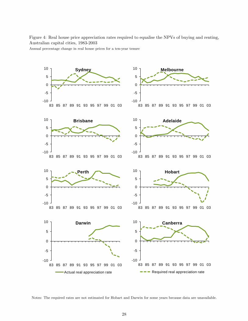
Figure 4: Real house price appreciation rates required to equalise the NPVs of buying and renting,Australian capital cities, 1983-2003Annual percentage change in real house prices for a ten-year tenure

-10

-5

0

5

10

83 85 87 89 91 93 95 97 99 01 03

Sydney

-10

-5

0

5

10

83 85 87 89 91 93 95 97 99 01 03

Melbourne

-10

-5

0

5

10

83 85 87 89 91 93 95 97 99 01 03

Brisbane

-10

-5

0

5

10

83 85 87 89 91 93 95 97 99 01 03

Adelaide

-10

-5

0

5

10

83 85 87 89 91 93 95 97 99 01 03

Perth

-10

-5

0

5

10

83 85 87 89 91 93 95 97 99 01 03

Hobart

-10

-5

0

5

10

83 85 87 89 91 93 95 97 99 01 03

Darwin

Actual real appreciation rate

-10

-5

0

5

10

83 85 87 89 91 93 95 97 99 01 03

Canberra

Required real appreciation rate

Notes: The required rates are not estimated for Hobart and Darwin for some years because data are unavailable.

28

Figure 5: Proportion of years where buying was optimal, by tenure length and renter’s investmentportfolio, 1983–2013Tenure lengths from 1-20 years. Three different investment portfolios

0

25

50

75

100

1 3 5 7 9 11 13 15 17 19

bu

y o

pti

mal (%

yrs

)

Sydney

0

25

50

75

100

1 3 5 7 9 11 13 15 17 19

bu

y o

pti

mal (%

yrs

)

Melbourne

0

25

50

75

100

1 3 5 7 9 11 13 15 17 19

bu

y o

pti

mal (%

yrs

)

Brisbane

0

25

50

75

100

1 3 5 7 9 11 13 15 17 19

bu

y o

pti

mal (%

yrs

)

Adelaide

0

25

50

75

100

1 3 5 7 9 11 13 15 17 19

bu

y o

pti

mal (%

yrs

)

Perth

0

25

50

75

100

1 3 5 7 9 11 13 15 17 19

bu

y o

pti

mal (%

yrs

)

Hobart

0

25

50

75

100

1 3 5 7 9 11 13 15 17 19

bu

y o

pti

mal (%

yrs

)

Darwin

100 per cent in shares

50 per cent in shares and 50 percent in term deposits

0

25

50

75

100

1 3 5 7 9 11 13 15 17 19

bu

y o

pti

mal (%

yrs

)

Canberra

100 per cent in term deposits

29

Figure 6: User cost of housing 1988–2004, five year tenure lengthOur estimates (solid lines), Brown et al. (2011) (dotted lines)

-10

-5

0

5

10

15

20

25

1988 1990 1992 1994 1996 1998 2000 2002 2004

Pe

r c

en

t

Sydney Melbourne Brisbane

Sydney Melbourne Brisbane

Notes: Estimates from Brown et al. are for an owner-occupier with an average income purchasing a property and

expecting to hold it for five years.

Table 4: Results from the switching analysis, Australian capital cities, 1983–2013

Sydney Melb. Bris. Adel. Perth Hobart Darwin Canb.

1983–2003 Buy Buy Rent/buy Buy Rent/buy ne ne Rent/buy(20) (20) (4/16) (20) (4/16) (16/4)

1985–2005 Buy Rent/buy Buy Rent/buy Buy/rent ne ne Rent/buy(20) (12/8) (20) (12/8) (4/16) (12/8)

1987–2007 Buy/rent Buy/rent Buy Rent/buy Rent/buy Rent/buy ne Rent/buy(16/4) (16/4) (20) (12/8) (12/8) (12/8) (12/8)

1989–2009 Rent/buy Rent/buy Rent/buy Rent/buy Rent/buy Rent/buy ne Rent/buy(8/12) (8/12) (8/12) (8/12) (8/12) (12/8) (8/12)

1991–2011 Rent/buy Rent/buy Rent/buy Rent/buy Rent/buy Rent/buy ne Rent/buy(4/16) (4/16) (8/12) (8/12) (8/12) (8/12) (8/12)

1993–2013 Buy/rent Rent/buy Rent/buy Rent/buy Rent/buy Rent/buy ne Rent/buy(12/8) (4/16) (4/16) (4/16) (8/12) (8/12) ne (4/16)

Notes: ‘ne’: not estimated due to data unavailability. The entry ’Buy/rent (16/4)’ means that buying the property

and holding it for 16 years and then switching to renting a property of equivalent quality for 4 years is financially

optimal for this 20-year period and for this city.

30

Figure 7: Is buying or renting currently optimal?10 year tenure length, renter invests half of their portfolio in shares and half in term deposits

0%

25%

50%

75%

100%

Syd. Melb. Brisb. Adel. Perth Hob. Dar. Canb. Total

Pe

r c

en

t o

f s

ce

na

rio

s

Buying optimal Renting optimal

31