An iterated local search algorithm based on nonlinear

programming for the irregular strip packing

problem

Takashi Imamichi a,∗, Mutsunori Yagiura b, Hiroshi Nagamochi a

aDepartment of Applied Mathematics and Physics, Graduate School of Informatics,

Kyoto University, Yoshida hommachi, Sakyo-ku, Kyoto 606-8501, Japan

bDepartment of Computer Science and Mathematical Informatics, Graduate School of

Information Science, Nagoya University, Furocho, Chikusa-ku, Nagoya 464-8603, Japan

February 07, 2007

Technical Report 2007-009

Abstract

The irregular strip packing problem is a combinatorial optimization problem that asks to

place a given set of 2-dimensional polygons within a rectangular container so that no poly-

gon overlaps with other polygons or protrudes from the container, where each polygon is

not necessarily convex. The container has a fixed width, while its length can change so that

all polygons are placed in it. The objective is to find a layout of the set of polygons that

minimizes the length of the container.

We propose an algorithm that separates overlapping polygons based on nonlinear pro-

gramming, and an algorithm that swaps two polygons in a layout so as to find their new

positions in the layout with the least overlap. We incorporate these algorithms as com-

ponents in an iterated local search algorithm for the overlap minimization problem and

then develop an algorithm for the irregular strip packing problem using the iterated local

search algorithm. Computational comparisons on representative instances disclose that our

algorithm is competitive with other existing algorithms. Moreover, our algorithm updates

several best known results.

Key words: irregular strip packing problem, iterated local search, no-fit polygon,

unconstrained nonlinear programming

∗ Corresponding author. Tel.: +81-75-753-5514; fax: +81-75-753-5514.

Email addresses: ima@amp.i.kyoto-u.ac.jp (Takashi Imamichi),

yagiura@nagoya-u.jp (Mutsunori Yagiura), nag@amp.i.kyoto-u.ac.jp (Hiroshi

Nagamochi).

1 Introduction

The irregular strip packing problem is a combinatorial optimization problem that

asks to place a given set of 2-dimensional polygons within a rectangular container,

where each polygon is not necessarily convex, so that no polygon overlaps with

other polygons or protrudes from the container. We say such a layout is feasible.

The container has a fixed width, while its length can change so that all polygons are

placed in it. The objective is to find a feasible layout that minimizes the length of

the container. The irregular strip packing problem has a few variations depending

on rotations of polygons: (1) rotations of any angle are allowed, (2) finite number of

angles are allowed, (3) no rotation is allowed. Among them, we deal with case (2)

in this paper. Note that case (3) is a special case of (2) in which the number of

given orientations for each polygon is one. The irregular strip packing problem has

many applications in material industry such as paper and textile industries, where

raw materials are usually given in rolls. In textile industry, rotations are usually

restricted to 180 degrees because textiles have the grain and may have a drawing

pattern. The irregular strip packing problem is known to be NP-hard even without

rotation [1].

Adamowicz and Albano [2] proposed an algorithm that first partitions given poly-

gons into several subsets of polygons, then generates for each of the subsets a rect-

angle enclosure in which the polygons in the subset are placed compactly (i.e.,

being with a little wasted space), and finally finds a layout of these enclosures. Al-

bano and Sapuppo [3] gave an algorithm that places given polygons one by one at

the bottom-left position according to a sequence of the input polygons, where they

used tree search to obtain a good sequence. Some approaches for finding a good

sequence are based on local search [4,5].

Mathematical programming was also used for the irregular strip packing problem.

Compaction and separation algorithms based on linear programming have been

proposed, e.g., by Li and Milenkovic [6], Bennell and Dowsland [7], and Gomes

and Oliveira [8]. Given a feasible layout of the given polygons, a compaction al-

gorithm translates the polygons in the current layout continuously in order to min-

imize the length of the container, and it outputs a locally optimal solution. Given

an infeasible layout of the given polygons, a separation algorithm translates the

polygons in the current layout continuously in order to make the layout feasible, it

also outputs a locally optimal solution.

Bennell and Dowsland [7] combined the bottom-left method and the LP based com-

paction algorithm to obtain a better algorithm. Gomes and Oliveira [8] hybridised

the bottom-left heuristic and the LP based compaction and separation algorithms.

They further incorporated the method with simulated annealing, and the resulting

algorithm updated many best known results on the benchmark instances of the ir-

regular strip packing problem. Burke et al. [9] developed a bottom-left fill heuristic

2

algorithm, and utilized it with hill climbing or tabu search to obtain good solutions

quickly. Egeblad et al. [10] developed an efficient method that finds a position of a

specified polygon that minimizes its overlap with the current layout when we trans-

late the polygon and they utilized it in guided local search. See a review by Hopper

and Turton [11] for more on the strip packing problem including the irregular strip

packing problem.

In this paper, we propose a new separation algorithm based on nonlinear program-

ming. We also give an algorithm that swaps two polygons to find their new positions

with small overlap provided that the positions of other polygons in a given layout

are fixed. We incorporate these algorithms as components in an iterated local search

algorithm whose objective is to minimize the total amount of overlap and protrusion

of a layout, where a layout may not be completely contained in the container during

the algorithm. We then develop an algorithm for the irregular strip packing prob-

lem using the iterated local search algorithm, which we call ILSQN because we

use the quasi-Newton method in the iterated local search algorithm. Computational

comparisons on representative benchmark instances disclose that our algorithm is

competitive with other existing algorithms. Moreover, our algorithm updates sev-

eral best known results.

This paper is organized as follows. We formulate the irregular strip packing prob-

lem and illustrate our approach to this problem in Section 2. We then define func-

tions that measure the amount of overlap and show how to evaluate these functions

and their gradients in Section 3. We explain our iterated local search algorithm for

the overlap minimization problem in Section 4 and give two procedures used in the

iterated local search algorithm: the separation algorithm based on nonlinear pro-

gramming and the operation of swapping two polygons in Section 5 and Section 6,

respectively. Finally we show the computational results in Section 7 and make a

concluding remark in Section 8.

2 Formulation and Approach

This section gives a mathematical formulation of the irregular strip packing prob-

lem and then illustrate an overview of our approach to the problem. For the irregu-

lar strip packing problem, we are given a list P = (P1, . . . , Pn) of polygons, a list

O = O1 × · · · ×On of the polygons’ orientations, where Oi (1 ≤ i ≤ n) is a set of

orientations in which Pi can be rotated, and a rectangular container C = C(W,L)with a width W ≥ 0 and a length L, where W is a constant and L is a nonnegative

variable. Polygons in P may not be convex.

We denote polygon Pi ∈ P rotated by o ∈ Oi degrees by Pi(o), which may be

written as Pi for simplicity when the orientation is not specified or clear from the

context. For convenience, we regard each of polygons Pi(o) (i = 1, . . . , n) and

3

rectangle C as the set of points inside it including the points on the boundary.

For a polygon S, let int(S) be the interior of S, ∂S be the boundary of S, S be

the complement of S, and cl(S) be the closure of S. We describe translations of

polygons by Minkowski sums. Let xi = (xi1, xi2) (i = 1, . . . , n) be a translation

vector for Pi. Thus the polygon obtained by translating polygon Pi by xi is Pi ⊕xi = {p + xi | p ∈ Pi}. Recall that L ≥ 0 is the length of the container C, which

is a decision variable to be minimized. Then the irregular strip packing problem is

formally described as follows:

minimize L

subject to int(Pi(oi) ⊕ xi) ∩ (Pj(oj) ⊕ xj) = ∅, 1 ≤ i < j ≤ n,

(Pi(oi) ⊕ xi) ⊆ C(W,L), 1 ≤ i ≤ n,

L ∈ R+,

oi ∈ Oi, 1 ≤ i ≤ n,

xi ∈ R2, 1 ≤ i ≤ n.

(1)

We represent a solution of problem (1) with a pair of n-tuples x = (x1, . . . ,xn)and o = (o1, . . . , on). Note that a solution (x,o) uniquely determines the layout

of the polygons. The minimum length L of the container C is formally defined by

function

µ(x,o) = max{x1 | (x1, x2) ∈ Pi(oi) ⊕ xi, Pi ∈ P}

− min{x1 | (x1, x2) ∈ Pi(oi) ⊕ xi, Pi ∈ P}.(2)

Figure 1 shows an example of a feasible layout of polygons. The length L is decided

as described by (2).PSfrag replacements

x

y

O

W

L

P1

P2

P3

P4

P5

P6

Fig. 1. An example of a feasible layout of six polygons in container C(W,L) (O is the

origin).

4

2.1 Overlap Minimization Problem

The problem (1) contains three types of variables, L, x and o. To construct an algo-

rithm as a building block of the entire algorithm to problem (1), we first introduce

the overlap minimization problem, a problem to find a feasible solution in con-

tainer C with a fixed length L. For this purpose, we allow solutions to have some

polygons which overlap each other and/or protrude from the container; the amount

of overlap and protrusion is penalized in such a way that a solution with penalty

zero gives a feasible layout to the current container. More specifically, for a pair

x = (x1, . . . ,xn) and o = (o1, . . . , on) of lists of translation vectors and orienta-

tion vectors of all polygons, let fij(x,o) be a function that measures the amount of

overlap of Pi(oi) and Pj(oj), and gi(x,o) be a function that measures the amount

of protrusion of Pi(oi) from the container. Then the overlap minimization problem

is formulated by

minimize F (x,o) =∑

1≤i<j≤n

fij(x,o) +∑

1≤i≤n

gi(x,o)

subject to x ∈ R2n, o ∈ O.

(3)

To design an effective procedure for the overlap minimization problem (3) is the

heart of our algorithm.

Note that the problem (3) is an unconstrained nonlinear programming problem.

However, we do not attempt to solve this problem by using an algorithm such as

quasi-Newton method since evaluation of functions fij and gi and their gradients

would be involved due to variables o for rotation. When we treat only variables x

for translation, evaluation of suitably defined functions fij and gi becomes much

easier by using an efficient data structure, called no-fit polygons, as will be dis-

cussed in Section 3. Given a solution (x,o), we fix the orientation o, and introduce

the following problem of translating polygons to reduce the total overlap, which is

called the polygon separation problem:

minimize F (x) =∑

1≤i<j≤n

fij(x) +∑

1≤i≤n

gi(x)

subject to x ∈ R2n,

(4)

where we omit indication of o for simplicity, A separation algorithm is obtained

by applying quasi-Newton method to this unconstrained nonlinear programming

problem (4). Thus the algorithm translates all polygons simultaneously to obtain a

locally optimal solution.

Since the separation algorithm only translates polygons, we need a procedure for

changing the orientations of polygons. For this, we design a swapping procedure

that changes the positions and orientations of two specified polygons to find their

best positions and orientations under the condition that the positions and orienta-

tions of the other polygons are fixed.

5

By combining the separation algorithm and the swapping procedure, we construct

an iterated local search algorithm, called MINIMIZEOVERLAP, to find a solution to

the overlap minimization problem (3). Given the current layout (xcur,ocur), MINI-

MIZEOVERLAP(P, O, C(W,L), xcur, ocur) outputs a new layout (x∗,o∗), which is

a locally optimal solution to the problem (3). The details of MINIMIZEOVERLAP

will be given in Section 4.

2.2 Entire Algorithm for the Irregular Strip Packing Problem

In this subsection, we give an entire description of algorithm ILSQN for prob-

lem (1). ILSQN first generates an initial solution by a method which we will ex-

plain in Section 6.4, and sets the length L of the container so that it contains all

polygons and the both sides touch some polygons. Then ILSQN repeats two layers

of computations until a time limit is reached. The outer layer is to search the mini-

mum feasible length L∗ by shrinking or extending the left and/or right sides of the

container. For the current layout (xcur,ocur), the outer layer chooses a length L of

the container, where (xcur,ocur) may be infeasible to the tentatively fixed length L.

The inner layer then improves the current solution (xcur,ocur) into a locally optimal

solution for the new length L. To find such a solution, the inner layer invokes MIN-

IMIZEOVERLAP. Figure 2 illustrates the behavior of the algorithm, where “shrink”

corresponds to the outer layer and “relocate” corresponds to the inner layer.

PSfrag replacementsinitial solution shrink

shrink relocate

relocate

Fig. 2. Two layers of algorithm ILSQN

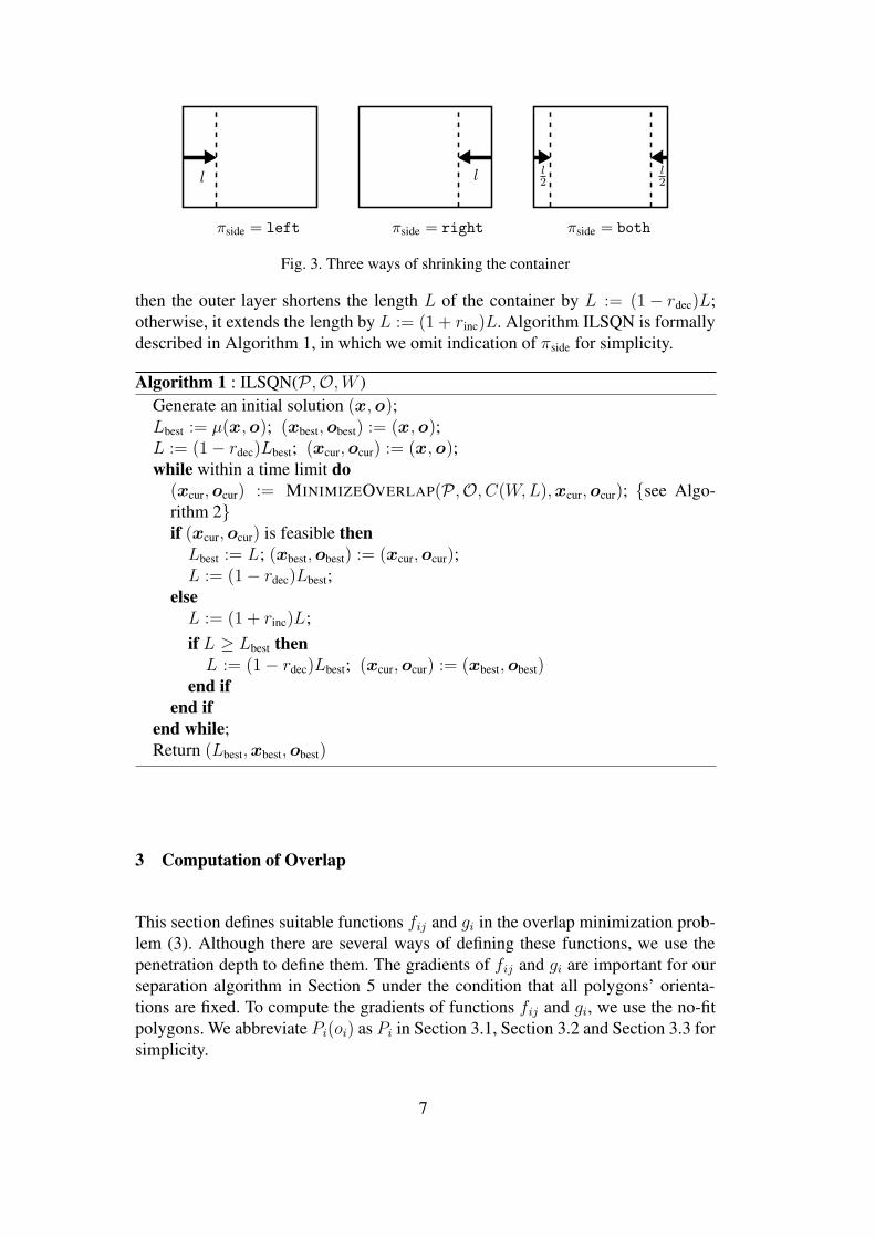
We now explain how to execute the outer layer. The execution of the outer layer

is described by parameters rdec ∈ (0, 1), rinc ∈ (0, 1) and πside ∈ {left, right,both}. We shrink and extend the length L of the container by factors rdec and

rinc, respectively. Parameter πside determines which side of the container we shrink

or extend. To be more precise, when ILSQN changes L to L − l, it translates the

container to the right by l, 0, and l/2 if πside = left, right, and both, respectively,

as shown in Figure 3.

After computing an initial solution (x,o), we shorten L by L := (1 − rdec)µ(x,o),and execute the inner layer. If the inner layer obtains a feasible layout successfully,

6

PSfrag replacements

πside = left πside = right πside = both

l l l2

l2

Fig. 3. Three ways of shrinking the container

then the outer layer shortens the length L of the container by L := (1 − rdec)L;

otherwise, it extends the length by L := (1 + rinc)L. Algorithm ILSQN is formally

described in Algorithm 1, in which we omit indication of πside for simplicity.

Algorithm 1 : ILSQN(P,O,W )

Generate an initial solution (x,o);Lbest := µ(x,o); (xbest,obest) := (x,o);L := (1 − rdec)Lbest; (xcur,ocur) := (x,o);while within a time limit do

(xcur,ocur) := MINIMIZEOVERLAP(P,O, C(W,L),xcur,ocur); {see Algo-

rithm 2}if (xcur,ocur) is feasible then

Lbest := L; (xbest,obest) := (xcur,ocur);L := (1 − rdec)Lbest;

else

L := (1 + rinc)L;

if L ≥ Lbest then

L := (1 − rdec)Lbest; (xcur,ocur) := (xbest,obest)end if

end if

end while;

Return (Lbest,xbest,obest)

3 Computation of Overlap

This section defines suitable functions fij and gi in the overlap minimization prob-

lem (3). Although there are several ways of defining these functions, we use the

penetration depth to define them. The gradients of fij and gi are important for our

separation algorithm in Section 5 under the condition that all polygons’ orienta-

tions are fixed. To compute the gradients of functions fij and gi, we use the no-fit

polygons. We abbreviate Pi(oi) as Pi in Section 3.1, Section 3.2 and Section 3.3 for

simplicity.

7

3.1 No-Fit Polygon

The no-fit polygon (NFP) is a data structure that is often used in algorithms for

the irregular strip packing problem [2–5,7,8]. It is also used for other problems

such as robotics, in which the no-fit polygon is called configuration-space obstacle.

Practical algorithms to calculate an NFP of two non-convex polygons have been

proposed, e.g., by Bennell et al. [12] and Ramkumar [13].

The no-fit polygon NFP(Pi, Pj) for an ordered pair of two polygons Pi and Pj is

defined by

NFP(Pi, Pj) = int(Pi) ⊕ (− int(Pj)) = {v − w | v ∈ int(Pi), w ∈ int(Pj)}.

The no-fit polygon has the following important properties:

• Pi ⊕ xi and Pj ⊕ xj overlap if and only if xj − xi ∈ NFP(Pi, Pj).• Pi ⊕ xi touches Pj ⊕ xj if and only if xj − xi ∈ ∂ NFP(Pi, Pj).• Pi ⊕ xi and Pj ⊕ xj are separated if and only if xj − xi 6∈ cl(NFP(Pi, Pj)).

Hence the problem of checking whether two polygons overlap or not becomes an

easier problem of checking whether a point is in a polygon or not. When Pi and Pj

are both convex, ∂ NFP(Pi, Pj) can be computed by the following simple proce-

dure. We first place the reference point of Pi at the origin, and slide Pj around Pi,

i.e., translate Pj having it keep touching with Pi. Then the trace of the reference

point of Pj is ∂ NFP(Pi, Pj). Figure 4 shows an example of NFP(Pi, Pj) of two

polygons Pi and Pj .

We can also check whether a polygon Pi protrudes from the container C or not by

using

NFP(C,Pi) = int(C) ⊕ (− int(Pi)) = {v − w | v ∈ R2 \ C, w ∈ int(Pi)},

which is the complement of a rectangle whose boundary is the trajectory of the

reference point of Pi when we slide Pi inside the container C. See an example in

Figure 5. The following properties are derived from those of the no-fit polygon:

• Pi ⊕ xi protrudes from C if and only if xi ∈ NFP(C,Pi).• Pi ⊕ xi is contained in C and touches ∂C if and only if xi ∈ ∂ NFP(C,Pi).• Pi ⊕ xi is contained in C and does not touch ∂C if and only if

xi 6∈ cl(NFP(C,Pi)).

To check if a polygon Pi ⊕ xi protrudes from C, Gomes and Oliveira [4,8] intro-

duced the inner-fit rectangle, which is equivalent to NFP(C,Pi).

8

PSfrag replacements

NFP(Pi, Pj)

Pi

Pi Pj

xixj

O

Fig. 4. Illustration of NFP(Pi, Pj) (O is the origin)PSfrag replacements

O

NFP(C,Pi)

IFR(C,Pi)

Pi

xi

Pi

Pj

C

C

Fig. 5. Illustration of NFP(C,Pi)

3.2 Penetration Depth

The penetration depth (also known as the intersection depth) is an important no-

tion used for robotics, computer vision and so on [14–16]. The penetration depth

δ(Pi, Pj) of two overlapping polygons Pi and Pj is defined to be the minimum

translational distance to separate them. If two polygons do not overlap, their pene-

tration depth is defined to be zero. Formally, the penetration depth of two polygons

Pi and Pj is defined by

δ(Pi, Pj) = min{‖z‖ | int(Pi) ∩ (Pj ⊕ z) = ∅, z ∈ R2},

where ‖ · ‖ denotes the Euclidean norm.

We can separate two polygons Pi and Pj by translating the reference point of Pj to a

point on ∂ NFP(Pi, Pj). Hence δ(Pi ⊕ xi, Pj ⊕ xj) is the minimum distance from

xj −xi to ∂ NFP(Pi, Pj). Figure 6 shows the relationship between the penetration

depth and the NFP. The solid and dashed arrows are examples of translations to the

boundary of the NFP and the dotted polygons are the polygons of Pj translated by

the vectors represented by these arrows. The solid arrow has the minimum distance

among all translations, giving the penetration depth δ(Pi ⊕ xi, Pj ⊕ xj).

9

PSfrag replacements PiPj

xixj

NFP(Pi, Pj)

Fig. 6. The no-fit polygon NFP(Pi ⊕ xi, Pj ⊕ xj) and the penetration depth

δ(Pi ⊕ xi, Pj ⊕ xj)

3.3 Amount of Overlap

We define functions fij and gi in problem (3) using the penetration depth. To rep-

resent the amount of overlap between Pi and Pj , we define fij by

fij(x) = δ(Pi ⊕ xi, Pj ⊕ xj)m, 1 ≤ i < j ≤ n,

where x = (x1, . . . ,xn) and m is a positive parameter. Similarly we define gi(x)by

gi(x) = δ(cl(C), Pi ⊕ xi)m

, 1 ≤ i ≤ n.

In order to apply efficient algorithms for solving the nonlinear program to the poly-

gon separation problem (4), we need to compute the values of fij(x) and gi(x) and

their gradients for a given solution (x,o), where all polygons’ orientations o are

fixed. We explain below how we realize such computation. Let xi and xj be the

translation vectors of Pi and Pj , respectively, and denote v = xj − xi for conve-

nience. We first consider how to compute fij(x) and ∇fij(x), and later explain the

case of gi(x) and ∇gi(x). There are three cases for the computation of fij(x) and

∇fij(x).

Case 1: two polygons Pi and Pj do not overlap. In this case, we see that fij(x) = 0and ∇fij(x) = 0.

Case 2: two polygons Pi and Pj overlap (i.e., fij(x) > 0) and the nearest point on

∂ NFP(Pi, Pj) from v is unique. See an example in Figure 7. Let w be the nearest

point and let z = w−v. Because the variable x is a list of n 2-dimensional vectors,

∇fij(x) is also such a list; hence we denote ∇fij(x) = (∇1fij(x), . . . ,∇nfij(x)),where ∇k = (∂/∂xk1, ∂/∂xk2), 1 ≤ k ≤ n. Then, fij(x) and ∇fij(x) for 1 ≤ i <

10

j ≤ n are given by

fij(x) = ‖z‖m,

∇ifij(x) = −∇jfij(x) = m‖z‖m−2z, (5)

∇kfij(x) = 0, k ∈ {1, . . . , n} \ {i, j}.

Every ∇kfij(x) except ∇ifij(x) and ∇jfij(x) is zero because only Pi and Pj have

influence on their overlap.PSfrag replacements

PiPj

NFP(Pi, Pj)

v = xj − xiw

xixj

Fig. 7. The computation of fij(x) and ∇fij(x)

Case 3: fij(x) > 0 and the nearest point from v to ∂ NFP(Pi, Pj) is not unique.

In this case, ∇fij is not differentiable at x; however, we choose one of the nearest

points arbitrarily as w and calculate ∇fij(x) with (5) as in Case 2.

Case 2 and Case 3 are distinguished in reference to the medial axis [17,18] of

NFP(Pi, Pj). The medial axis of a polygon P is defined by the trace of the centers

of all circles contained in P that touch at least two sides of ∂P . Figure 8 shows

an example of an NFP and its medial axis. The thick solid polygon is an NFP,

s1, . . . , s7 are the edges of the NFP, and the dashed lines are the medial axis of the

NFP. For the two points v1 and v2, the arrows indicate the nearest point on the

NFP from v1 and v2, respectively. The nearest point on the NFP’s boundary from

a point v in the NFP is unique if and only if v is not on the medial axis of the NFP.

In Figure 8, v1 is not on the medial axis and it has the unique nearest point on s3.

On the other hand v2 is on the medial axis and it has two nearest points on s1 and

s2. Note that v can have more than one nearest point only when v is on the medial

axis of the NFP. Such a case is rare because the search basically tries to change v

so that it moves away from the medial axis in order to minimize the sum of fij(x).

We compute gi(x) and ∇gi(x) similarly as in the case of fij(x) and ∇fij(x).If Pi is contained in C, we simply return gi(x) = 0 and ∇gi(x) = 0. We con-

sider a polygon Pi that protrudes from the container C (i.e., gi(x) > 0). See an

example in Figure 9. Let w be the nearest point on ∂ NFP(C,Pi) from xi and

z = w − xi; the nearest point is always unique in this case. We denote ∇gi(x) =(∇1gi(x), . . . ,∇ngi(x)). Then, gi(x) and its gradient for 1 ≤ i < j ≤ n are given

11

PSfrag replacements

s1

s2

s3

s4

s5s6

s7

v1

v2

Fig. 8. The medial axis of an NFP and the nearest points on the boundary from inner points

v1 and v2

by

gi(x) = ‖z‖m,

∇igi(x) = −m‖z‖m−2z, (6)

∇kgi(x) = 0, k ∈ {1, . . . , n} \ {i}.

Every ∇kgi(x) except ∇igi(x) is zero because only Pi has influence on its protru-

sion from the container.

PSfrag replacements Pi

C

NFP(C,Pi) xi

wxi

Fig. 9. The computation of gi(x) and ∇gi(x)

In Case 2, fij(x) is not differentiable at x if and only if Pi and Pj touch each

other and 0 < m ≤ 1. Similarly gi(x) is not differentiable at x if and only if Pi is

contained in C, touches C and 0 < m ≤ 1. We avoid choosing such m as will be

discussed below. We can thus calculate the gradient of the objective function of (3).

The positive parameter m determines the differentiability of fij(x) and gi(x). Fig-

ure 10 shows the change of fij(x) along the arrow from the outside to the inside

of an NFP. At the boundary of the NFP, fij(x) is indifferentiable for 0 < m ≤ 1,

while it is differentiable for m > 1. Moreover, ∇fij(x) in (5) becomes simpler for

m = 2 because ‖z‖m−2 disappears. The situation is the same for gi(x), and hence

we let m = 2 in our experiments.

12

PSfrag replacements

A

NFP

PSfrag replacements

A

NFP

fij(x) fij(x)fij(x)

0 < m < 1 m = 1 m > 1

Fig. 10. The value of fij(x) on arrow A

3.4 Computing NFPs for ILSQN

In the previous subsections, we show how to use no-fit polygons to evaluate func-

tions fij and gi and their gradients, where the orientations of polygons are fixed

for simplicity. However, in our algorithm ILSQN, we need to use no-fit polygons

NFP(Pi(oi), Pj(oj)) and NFP(C,Pi(oi)) for all possible orientations oi and oj .

We thus compute all NFP(Pi(oi), Pj(oj)), oi ∈ Oi, oj ∈ Oj , 1 ≤ i < j ≤ nbeforehand and utilize them in ILSQN.

4 Iterated Local Search for the Overlap Minimization Problem

In this section, we formally describe MINIMIZEOVERLAP, of our iterated local

search algorithm for the overlap minimization problem (3) introduced in Section 2.1.

MINIMIZEOVERLAP invokes the following algorithms, which we explain in detail

afterwards.

• SWAPTWOPOLYGONS: an operation of swapping two specified polygons in a

given layout considering rotations, where the other polygons and the length L of

the container are fixed. (The detail is given in Section 6.)

• SEPARATE: an algorithm that translates all polygons in a given layout simultane-

ously and (usually) slightly to reduce the total amount of overlap and protrusion,

where the length L of the container is fixed. It does not consider rotation. (The

detail is given in Section 5.)

MINIMIZEOVERLAP maintains the earliest solution that minimizes the objective

function F of (3) among those searched by then as the incumbent solution (xinc,oinc),which will be used for generating the next initial solution. MINIMIZEOVERLAP

13

first perturbs the incumbent solution by swapping two randomly chosen polygons

Pi and Pj calling SWAPTWOPOLYGONS(P,O, C, xinc,oinc, Pi, Pj), and then trans-

lates all polygons simultaneously calling SEPARATE(P,O, C,xinit,oinit) to obtain a

locally optimal solution (xlopt,olopt) of (3). Since SEPARATE does not rotate poly-

gons, olopt = oinit holds. If the locally optimal solution has less overlap than the

incumbent solution does, we update the incumbent solution with the locally opti-

mal solution. MINIMIZEOVERLAP stops these operations if it fails to update the

incumbent solution after a prescribed number Nmo of consecutive calls to local

search. The algorithm is formally described in Algorithm 2, where (xinc,oinc) is an

initial layout given to the algorithm.

Algorithm 2 : MINIMIZEOVERLAP(P,O, C,xinc,oinc)

k := 0;

while k < Nmo do

Randomly choose Pi and Pj from P;

(xinit,oinit) := SWAPTWOPOLYGONS(P,O, C,xinc,oinc, Pi, Pj);(xlopt,olopt) := SEPARATE(P,O, C,xinit,oinit);k := k + 1;

if F (xlopt,olopt) < F (xinc,oinc) then

(xinc,oinc) := (xlopt,olopt);k := 0

end if

end while;

Return (xinc,oinc)

5 Separation Algorithm

This section describes our separation algorithm SEPARATE, which is used as local

search in MINIMIZEOVERLAP. The polygon separation problem (4) introduced in

Section 2.1 is an unconstrained nonlinear programming problem, where all poly-

gons’ orientations o and the length L of the container are fixed. The objective func-

tion F of (4) and its gradient ∇F are efficiently computable because ∇fij and ∇gi

are computable with the no-fit polygons as described in Section 3.3. SEPARATE(P,O, C, x, o) is thus realized as follows: SEPARATE first applies the quasi-Newton

method to the polygon separation problem (4) by using the current layout (x,o)as an initial solution and SEPARATE returns a locally optimal solution delivered by

the quasi-Newton method. SEPARATE translates all polygons simultaneously and

(usually) slightly to reduce the total amount of overlap and protrusion, where no

rotation is considered. The idea is natural; however, to the best of our knowledge, it

seems that nonlinear programming approaches of this type have not been success-

fully applied.

14

6 Swapping Two Polygons

6.1 Moving a Polygon

ILSQN perturbs a locally optimal solution by swapping two polygons in the solu-

tion. Instead of just exchanging two polygons Pi and Pj in their reference points,

we attempt to find their positions with the least overlap. FINDBESTPOSITION(P,O, C, x, o, Pi) is a heuristic algorithm to find a minimum overlap position of a

specified polygon Pi without changing the positions of the other polygons, while

considering all possible orientations o ∈ Oi of Pi. Let N (o) be the set of polygon

boundaries ∂ NFP(Pk(ok)⊕xk, Pi(o)), Pk ∈ P \{Pi} and ∂ NFP(C,Pi(o)), V(o)be the set of vertices of N (o), and I(o) be the set of edge intersections of N (o). For

each point v ∈ V(o) ∪ I(o), the heuristics computes the overlap of Pi(o) ⊕ v with

the other polygons, and finds the position with the least overlap, where x is a list of

the translation vectors of polygons, o is a list of the orientations of polygons, and

the amount of overlap is computed by the objective function F (x,o) of the overlap

minimization problem (3). By repeating these operations for all orientations o ∈ Oi

of Pi, it seeks the best position and orientation. The algorithm is formally described

in Algorithm 3, where (x)i denotes the ith element of x and (o)i denotes the ithelement of o.

Algorithm 3 : FINDBESTPOSITION(P,O, C,x,o, Pi)

F ∗ := +∞;

for each o ∈ Oi do

Compute NFP(Pk(ok) ⊕ xk, Pi(o)) (Pk ∈ P \ {Pi}) and NFP(C,Pi(o));for each v ∈ V(o) ∪ I(o) do

x′ := x; (x′)i := v;

o′ := o; (o′)i := o;

if F (x′,o′) < F ∗ then

F ∗ := F (x′,o′); v∗ := v; o∗ := o

end if

end for

end for;

Return (v∗, o∗)

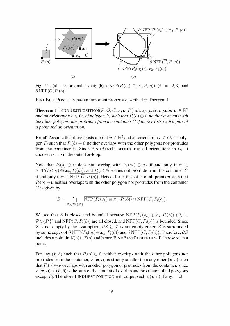
Figure 11 shows an example in which FINDBESTPOSITION is searching for the

best position for a square P1(o) with a fixed orientation o ∈ O1 in the left lay-

out. Figure 11(b) shows NFP(P2(o2)⊕ x2, P1(o)), NFP(P3(o3)⊕ x3, P1(o)), and

NFP(C,P1(o)). The circles in Figure 11(b) represent V(o) and I(o). FINDBEST-

POSITION finds a point that corresponds to a layout with the least overlap. Each

grey circle in Figure 11(b) corresponds to a position that has no overlap in Fig-

ure 11(a).

15

(a) (b)

PSfrag replacements

C

P1(o)

P2(o2)

P3(o3)

x2

x3

∂ NFP(P2(o2) ⊕ x2, P1(o))

∂ NFP(P3(o3) ⊕ x3, P1(o))

∂ NFP(C,P1(o))

Fig. 11. (a) The original layout; (b) ∂ NFP(Pi(oi) ⊕ xi, P1(o)) (i = 2, 3) and

∂ NFP(C,P1(o))

FINDBESTPOSITION has an important property described in Theorem 1.

Theorem 1 FINDBESTPOSITION(P,O, C,x,o, Pi) always finds a point v ∈ R2

and an orientation o ∈ Oi of polygon Pi such that Pi(o) ⊕ v neither overlaps with

the other polygons nor protrudes from the container C if there exists such a pair of

a point and an orientation.

Proof Assume that there exists a point v ∈ R2 and an orientation o ∈ Oi of poly-

gon Pi such that Pi(o) ⊕ v neither overlaps with the other polygons nor protrudes

from the container C. Since FINDBESTPOSITION tries all orientations in Oi, it

chooses o = o in the outer for-loop.

Note that Pi(o) ⊕ v does not overlap with Pk(ok) ⊕ xk if and only if v ∈NFP(Pk(ok) ⊕ xk, Pi(o)), and Pi(o) ⊕ v does not protrude from the container C

if and only if v ∈ NFP(C,Pi(o)). Hence, for o, the set Z of all points v such that

Pi(o)⊕ v neither overlaps with the other polygon nor protrudes from the container

C is given by

Z =⋂

Pk∈P\{Pi}

NFP(Pk(ok) ⊕ xk, Pi(o)) ∩ NFP(C,Pi(o)).

We see that Z is closed and bounded because NFP(Pk(ok) ⊕ xk, Pi(o)) (Pk ∈

P \{Pi}) and NFP(C,Pi(o)) are all closed, and NFP(C,Pi(o)) is bounded. Since

Z is not empty by the assumption, ∂Z ⊆ Z is not empty either. Z is surrounded

by some edges of ∂ NFP(Pk(ok)⊕xk, Pi(o)) and ∂ NFP(C,Pi(o)). Therefore, ∂Zincludes a point in V(o)∪I(o) and hence FINDBESTPOSITION will choose such a

point.

For any (v, o) such that Pi(o) ⊕ v neither overlaps with the other polygons nor

protrudes from the container, F (x,o) is strictly smaller than any other (v, o) such

that Pi(o)⊕v overlaps with another polygon or protrudes from the container, since

F (x,o) at (v, o) is the sum of the amount of overlap and protrusion of all polygons

except Pi. Therefore FINDBESTPOSITION will output such a (v, o) if any. 2

16

However, FINDBESTPOSITION may miss the globally optimal position if there is

no position whose overlap is zero.

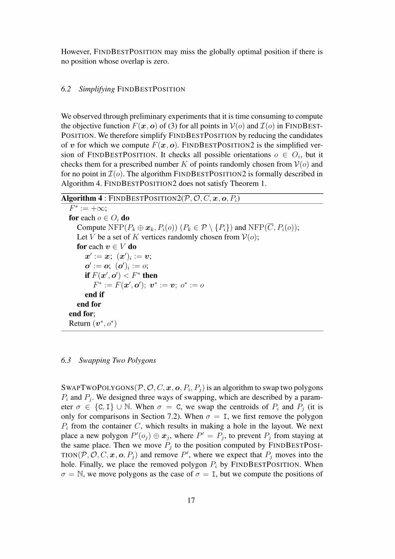
6.2 Simplifying FINDBESTPOSITION

We observed through preliminary experiments that it is time consuming to compute

the objective function F (x,o) of (3) for all points in V(o) and I(o) in FINDBEST-

POSITION. We therefore simplify FINDBESTPOSITION by reducing the candidates

of v for which we compute F (x,o). FINDBESTPOSITION2 is the simplified ver-

sion of FINDBESTPOSITION. It checks all possible orientations o ∈ Oi, but it

checks them for a prescribed number K of points randomly chosen from V(o) and

for no point in I(o). The algorithm FINDBESTPOSITION2 is formally described in

Algorithm 4. FINDBESTPOSITION2 does not satisfy Theorem 1.

Algorithm 4 : FINDBESTPOSITION2(P,O, C,x,o, Pi)

F ∗ := +∞;

for each o ∈ Oi do

Compute NFP(Pk ⊕ xk, Pi(o)) (Pk ∈ P \ {Pi}) and NFP(C,Pi(o));Let V be a set of K vertices randomly chosen from V(o);for each v ∈ V do

x′ := x; (x′)i := v;

o′ := o; (o′)i := o;

if F (x′,o′) < F ∗ then

F ∗ := F (x′,o′); v∗ := v; o∗ := o

end if

end for

end for;

Return (v∗, o∗)

6.3 Swapping Two Polygons

SWAPTWOPOLYGONS(P,O, C,x,o, Pi, Pj) is an algorithm to swap two polygons

Pi and Pj . We designed three ways of swapping, which are described by a param-

eter σ ∈ {C, I} ∪ N. When σ = C, we swap the centroids of Pi and Pj (it is

only for comparisons in Section 7.2). When σ = I, we first remove the polygon

Pi from the container C, which results in making a hole in the layout. We next

place a new polygon P ′(oj) ⊕ xj , where P ′ = Pj , to prevent Pj from staying at

the same place. Then we move Pj to the position computed by FINDBESTPOSI-

TION(P,O, C,x,o, Pj) and remove P ′, where we expect that Pj moves into the

hole. Finally, we place the removed polygon Pi by FINDBESTPOSITION. When

σ = N, we move polygons as the case of σ = I, but we compute the positions of

17

Pi and Pj by FINDBESTPOSITION2(P,O, C,x,o, Pj), where we set K = σ. The

algorithm SWAPTWOPOLYGONS is formally described in Algorithm 5, where (P)i

denotes the ith element of P and (O)i denotes the ith element of O. We compare

the three ways of swapping by computational experiments in Section 7.2.

Algorithm 5 : SWAPTWOPOLYGONS(P,O, C,x,o, Pi, Pj)

{For σ = C}for each (o′i, o

′j) ∈ Oi × Oj do

Swap Pi(o′i) and Pj(o

′j) at their centroids;

Let (x′,o′) be the resulting layout

end for;

Let (x,o) be the (x′,o′) with the minimum F (x′,o′) among those generated in

the above loop;

Return (x,o)

{For σ = I}P ′ := P; O′ := O; x

′ := x; o′ := o;

(P ′)i := (P)j; (O′)i := (o)j; (x′)i := (x)j; (o′)i := (o)j;

((x)j, (o)j) := FINDBESTPOSITION(P ′,O′, C,x′,o′, (P ′)j);((x)i, (o)i) := FINDBESTPOSITION(P,O, C,x,o, (P)i);Return (x,o)

{For σ ∈ N}P ′ := P; O′ := O; x

′ := x; o′ := o;

(P ′)i := (P)j; (O′)i := (o)j; (x′)i := (x)j; (o′)i := (o)j;

((x)j, (o)j) := FINDBESTPOSITION2(P ′,O′, C,x′,o′, (P ′)j);((x)i, (o)i) := FINDBESTPOSITION2(P,O, C,x,o, (P)i);Return (x,o)

6.4 Initial solution of ILSQN

We generate an initial feasible layout of ILSQN using FINDBESTPOSITION or

FINDBESTPOSITION2. We assume that the initial length L of the container C(W,L)is large enough to place all polygons in P without overlap in C. We prepare a se-

quence of polygons in P and place polygons one by one in the order of the se-

quence, where the position of each polygon Pi is decided by FINDBESTPOSITION

or FINDBESTPOSITION2. We control the sequence by using a parameter Sinit ∈{sort, random}: the sequence of the descending order of area if Sinit = sort and

a random sequence if Sinit = random. We use FINDBESTPOSITION if σ ∈ {C, I}and FINDBESTPOSITION2 if σ ∈ N, where we give σ to FINDBESTPOSITION2 as

the parameter K. If there are more than one position with no overlap, we choose

the bottom-left position (i.e., the position with the minimum xi1, breaking ties with

18

the minimum xi2, where xi = (xi1, xi2) is the translation vector of polygon Pi). We

compute the length L of the container by (2) after placing all polygons in P .

There are variations in choosing a sequence of polygons such as the descending

order of area and a random order. Gomes and Oliveira [8] also generated initial

solutions in a similar way using a different sequence of polygons.

7 Computational Results

This section reports the results on computational experiments of our algorithm

ILSQN and other algorithms.

7.1 Environment

Benchmark instances for the irregular strip packing problem are available online at

EURO Special Interest Group on Cutting and Packing (ESICUP) website. 1 Table 1

shows the information of the instances. The column NDP shows the number of dif-

ferent polygons, the column TNP shows the total number of polygons, the column

ANV shows the average number of the vertices of different polygons, the column

Orientations shows the permitted orientations, and the column Width shows the

width W of the container.

We implemented our algorithm ILSQN in C++, compiled it by GCC 4.0.2 and con-

ducted computational experiments on a PC with an Intel Xeon 2.8GHz processor

and 1GB memory. We adopt a quasi-Newton method package L-BFGS [19] for al-

gorithm SEPARATE. L-BFGS has a parameter mBFGS that is the number of BFGS

corrections in L-BFGS. We set mBFGS = 6 because 3 ≤ mBFGS ≤ 7 is recom-

mended in the L-BFGS package.

A layout is judged to be feasible when the objective function F (x,o) of (3) is

less than ε = 10−10W 2 due to limited precision. Thus, our algorithm may generate

layouts that have a slight overlap.

7.2 Parameters

ILSQN has the following parameters:

• rdec ∈ (0, 1): the ratio by which ILSQN shortens the container.

1 ESICUP: http://www.fe.up.pt/esicup/

19

Table 1

Information of instances (cited from [8])

Instance NDP TNP ANV Orientations (◦) Width

ALBANO 8 24 7.25 0, 180 4900

DAGLI 10 30 6.30 0, 180 60

DIGHE1 16 16 3.87 0 100

DIGHE2 10 10 4.70 0 100

FU 12 12 3.58 0, 90, 180, 270 38

JAKOBS1 25 25 5.60 0, 90, 180, 270 40

JAKOBS2 25 25 5.36 0, 90, 180, 270 70

MAO 9 20 9.22 0, 90, 180, 270 2550

MARQUES 8 24 7.37 0, 90, 180, 270 104

SHAPES0 4 43 8.75 0 40

SHAPES1 4 43 8.75 0, 180 40

SHAPES2 7 28 6.29 0, 180 15

SHIRTS 8 99 6.63 0, 180 40

SWIM 10 48 21.90 0, 180 5752

TROUSERS 17 64 5.06 0, 180 79

NDP: The number of different polygons

TNP: The total number of polygons

ANV: The average number of vertices of different polygons

• rinc ∈ (0, 1): the ratio by which ILSQN extends the container.

• πside ∈ {left, right, both}: the side of the container ILSQN shortens or ex-

tends.

• Nmo > 0: the termination criterion of MINIMIZEOVERLAP.

• Sinit ∈ {sort, random}: the sequence from which ILSQN generates an initial so-

lution. “Sinit = sort” means the descending order of area and “Sinit = random”

means a random sequence.

• σ ∈ {C, I}∪N: the ways of generating an initial solution in ILSQN and swapping

two polygons in SWAPTWOPOLYGONS.

In order to generate an initial solution, ILSQN uses FINDBESTPOSITION if

σ = I or C, and uses FINDBESTPOSITION2 if σ ∈ N, where σ ∈ N is the

parameter K of FINDBESTPOSITION2.

SWAPTWOPOLYGONS swaps the centroids of two given polygon if σ = C,

swaps them by FINDBESTPOSITION if σ = I, and swaps them by FINDBEST-

POSITION2 if σ ∈ N, where σ ∈ N is the parameter K of FINDBESTPOSI-

TION2.

We measure the efficiency of a solution by the ratio

the total area of the polygons

the area of the container.

20

We investigated the effects of the parameters by the following four computational

experiments. We choose six benchmark instances (SHAPES0, SHAPES1,

SHAPES2, SHIRTS, SWIM, TROUSERS), and conducted 5 runs with the time

limit of each run being 10 minutes.

We first checked the effect of πside. Figure 12 shows the average efficiency of five

runs; the graph on the left shows the result of Sinit = sort, and the one on the right

shows the result of Sinit = random, where we set rdec = 0.04, rinc = 0.01, Nmo =200, and σ = I. These results indicate that πside does not have much effect on the

efficiency.

65

70

75

80

85

90

95

bothrightleft

Effi

cien

cy (

%)

SHAPES0SHAPES1SHAPES2

SHIRTSSWIM

TROUSERS

PSfrag replacements

πside

65

70

75

80

85

90

95

bothrightleft

Effi

cien

cy (

%)

SHAPES0SHAPES1SHAPES2

SHIRTSSWIM

TROUSERS

PSfrag replacements

πside

Fig. 12. Average efficiencies against πside (left: Sinit = sort, right: Sinit = random)

We second checked the effect of rdec and rinc. Figure 13 shows the average effi-

ciency of five runs; the graph on the left shows the result of Sinit = sort, and the

one on the right shows the result of Sinit = random, where we set Nmo = 200,

πside = right, σ = I. From these results, we observe that the efficiency is almost

same for rdec ≤ 0.06.

Next, we checked the effect of Nmo. Figure 14 shows the average efficiency of five

runs; the graph on the left shows the result of Sinit = sort, and the one on the

right shows the result of Sinit = random, where we set rdec = 0.04, rinc = 0.01,

πside = right, and σ = I. These results indicate that the efficiency is slightly

better for 50 ≤ Nmo ≤ 300.

Finally, we checked the effect of σ. Figure 15 shows the average efficiency of five

runs; the graph on the left shows the result of Sinit = sort, and the one on the

right shows the result of Sinit = random, where we set rdec = 0.04, rinc = 0.01,

πside = right, and Nmo = 200. These results indicate that the efficiency is clearly

worse for σ = C, the efficiency is better for 100 ≤ σ ≤ 800, and the best result is

21

obtained when Sinit = sort and σ = 800. We can also observe from Figures 12–15

that Sinit does not have much effect on the efficiency.

Based on these observations, we set Sinit = sort, πside = right, rdec = 0.04,

rinc = 0.01, Nmo = 200, and σ = 800 for the computational experiments of all

benchmark instances in Section 7.3.

65

70

75

80

85

90

95

(10, 5)(10, 2.5)(8, 4)(8, 2)(6, 3)(6, 1.5)(4, 2)(4, 1)(2, 1)(2, 0.5)

Effi

cien

cy (

%)

SHAPES0SHAPES1SHAPES2

SHIRTSSWIM

TROUSERS

PSfrag replacements

(rdec, rinc)

65

70

75

80

85

90

95

(10, 5)(10, 2.5)(8, 4)(8, 2)(6, 3)(6, 1.5)(4, 2)(4, 1)(2, 1)(2, 0.5)

Effi

cien

cy (

%)

SHAPES0SHAPES1SHAPES2

SHIRTSSWIM

TROUSERS

PSfrag replacements

(rdec, rinc)

Fig. 13. Average efficiencies against (rdec, rinc) in % (left: Sinit = sort, right: Sinit =random)

65

70

75

80

85

90

95

200015001000800600400300200100502010

Effi

cien

cy (

%)

SHAPES0SHAPES1SHAPES2

SHIRTSSWIM

TROUSERS

PSfrag replacements

Nmo

65

70

75

80

85

90

95

200015001000800600400300200100502010

Effi

cien

cy (

%)

SHAPES0SHAPES1SHAPES2

SHIRTSSWIM

TROUSERS

PSfrag replacements

Nmo

Fig. 14. Average efficiencies against Nmo (left: Sinit = sort, right: Sinit = random)

7.3 Results

In this subsection, we show the computational results of our algorithm ILSQN com-

paring it with other existing algorithms. We ran algorithm ILSQN ten times for each

instances listed in Table 1 and compared our results with those reported by Gomes

and Oliveira [8] (denoted as “SAHA”), Burke et al. [9] (denoted as “BLF”) and Ege-

blad et al. [10] (denoted as “2DNest”). Table 2 shows the best and average length

and efficiency in % of ILSQN and the best efficiency in % of the other algorithms.

The column EF shows the efficiency in %. The best results among these algorithms

22

65

70

75

80

85

90

95

I20001500100080060040020010050C

Effi

cien

cy (

%)

SHAPES0SHAPES1SHAPES2

SHIRTSSWIM

TROUSERS

PSfrag replacements

σ

65

70

75

80

85

90

95

I20001500100080060040020010050C

Effi

cien

cy (

%)

SHAPES0SHAPES1SHAPES2

SHIRTSSWIM

TROUSERS

PSfrag replacements

σ

Fig. 15. Average efficiencies against σ (left: Sinit = sort, right: Sinit = random)

are written in bold typeface. Table 3 shows the computation time (in seconds) of

the algorithms.

Gomes and Oliveira [8] did not use time limit but stop their algorithm by other

criteria. They conducted 20 runs for each instance and the best results of the 20

runs are shown in Table 2, while their computation times in Table 3 are the average

computation time of the 20 runs.

Burke et al. [9] tested four variations of their algorithm, and conducted 10 runs for

each variation. Their results in Table 2 are the best results of the 40 runs, which are

taken from Table 5 in [9]. They limited the number of iterations for each run, and

their computation time in Table 3 is the time spent to find the best solution reported

in Table 2 in the run that found it (i.e., the time for only one run is reported). Since

they conducted experiments for instances ALBANO, DIGHE1 and DIGHE2 with

different orientations from the others, we do not include the results.

Egeblad et al. [10] and we conducted experiments using the time limits for each

run shown in Table 3.

Although our total computation time of all runs for each instance is not so long

compared with SAHA [8] and 2DNest [10], ILSQN obtained the best results for

8 instances out of the 15 instances in efficiency of the resulting layouts and also

obtained the results with almost equivalent efficiency to the best results for some

instances. It achieved the same efficiency as 2DNest [10] for instance SHAPES1,

but the layouts are different. The computation time of BLF [9] is much shorter than

that of ILSQN, and ILSQN obtained better results in efficiency than those BLF [9]

obtained for all instances. Figure 16 shows the best layouts obtained by ILSQN for

all instances.

23

JAKOBS1 JAKOBS2 MAO MARQUES

FU SHAPES2 DIGHE1 DIGHE2

SHAPES0 SHAPES1 DAGLI

ALBANO TROUSERS

SHIRTS SWIM

Fig. 16. The best solutions obtained by ILSQN

24

Table 2

The length of ILSQN and the efficiency in % of the four algorithms

Instance ILSQN SAHA [8] BLF [9] 2DNest [10]

Average Best Best Best Best

Length EF (%) Length EF (%) EF (%) EF (%) EF (%)

ALBANO 9990.23 87.14 9874.48 88.16 87.43 – 87.44

DAGLI 59.11 85.80 58.02 87.40 87.15 83.7 85.98

DIGHE1 110.69 90.49 100.11 99.89 100.00 – 99.86

DIGHE2 120.43 84.21 100.01 99.99 100.00 – 99.95

FU 32.56 87.57 31.43 90.67 90.96 86.9 91.84

JAKOBS1 11.56 84.78 11.28 86.89 †∗78.89 82.6 89.07

JAKOBS2 23.98 80.50 23.39 82.51 77.28 74.8 80.41

MAO 1813.38 81.31 1766.43 83.44 82.54 79.5 85.15

MARQUES 79.72 86.81 77.70 89.03 88.14 86.5 89.17

SHAPES0 60.02 66.49 58.30 68.44 66.50 60.5 67.09

SHAPES1 54.79 72.83 54.04 73.84 71.25 66.5 73.84

SHAPES2 26.44 81.72 25.64 84.25 83.60 77.7 81.21

SHIRTS 61.28 88.12 60.83 88.78 †86.79 84.6 86.33

SWIM 5928.23 74.62 5875.17 75.29 74.37 68.4 71.53

TROUSERS 245.58 88.69 242.56 89.79 89.96 88.5 89.84

∗ The value has been corrected from the one reported in [8] according to the information sent from

the authors of [8].† Better results were obtained by a simpler greedy approach (GLSHA)[8]: 81.67% for JAKOBS1

and 86.80% for SHIRTS.

8 Conclusions

We proposed an iterated local search algorithm for the overlap minimization prob-

lem consolidating a separation algorithm based on nonlinear programming and a

swapping operation of two polygons, and incorporated it in our algorithm ILSQN

for the irregular strip packing problem. We showed through computational experi-

ments that ILSQN is competitive with existing algorithms, updating the best known

solutions for several benchmark instances.

It is left as future work to combine our algorithm and the multi-stage approach [8]

to obtain better solutions quickly. For this approach, we need to develop an algo-

rithm to automatically cluster polygons by some criteria. It is also left to extend

our algorithm to handle rotations of any angle or other shapes such as those with

curved lines or 3-dimensional objects. Furthermore, computation of a good lower

bound of the irregular strip packing problem is also important to evaluate heuristic

algorithms or to develop exact algorithms.

25

Table 3

The computation time in seconds of the four algorithms

Instance ∗ILSQN †SAHA [8] ‡BLF [9] ∗2DNest [10]

Xeon Pentium4 Pentium4 Pentium4

2.8 GHz 2.4 GHz 2.0 GHz 3.0 GHz

10 runs 20 runs 4×10 runs 20 runs

ALBANO 1200 2257 – 600

DAGLI 1200 5110 188.80 600

DIGHE1 600 83 – 600

DIGHE2 600 22 – 600

FU 600 296 20.78 600

JAKOBS1 600 332 43.49 600

JAKOBS2 600 454 81.41 600

MAO 1200 8245 29.74 600

MARQUES 1200 7507 4.87 600

SHAPES0 1200 3914 21.33 600

SHAPES1 1200 10314 2.19 600

SHAPES2 1200 2136 21.00 600

SHIRTS 1200 10391 58.36 600

SWIM 1200 6937 607.37 600

TROUSERS 1200 8588 756.15 600

∗ Computation time is the time limit for each run.† Computation time is the average computation time.‡ Computation time is the time spent to find the best solution in the

run that found it.

Acknowledgements

This research was partially supported by a Scientific Grant in Aid from the Ministry

of Education, Science, Sports and Culture of Japan. We would like to thank Toshi-

hide Ibaraki, Shinji Imahori, Shunji Umetani, Koji Nonobe, and Nobuo Yamashita

for numbers of helpful comments and suggestions.

26

References

[1] B. K. Nielsen, A. Odgaard, Fast neighborhood search for the nesting problem,

Technical report 03/03, DIKU, Department of Computer Science, University of

Copenhagen (2003).

[2] M. Adamowicz, A. Albano, Nesting two-dimensional shapes in rectangular modules,

Computer-Aided Design 8 (1) (1976) 27–33.

[3] A. Albano, G. Sapuppo, Optimal allocation of two-dimensional irregular shapes using

heuristic search methods, IEEE Transactions on Systems, Man and Cybernetics SMC-

10 (5) (1980) 242–248.

[4] M. A. Gomes, J. F. Oliveira, A 2-exchange heuristic for nesting problems, European

Journal of Operational Research 141 (2) (2002) 359–370.

[5] J. F. Oliveira, A. M. Gomes, J. S. Ferreira, TOPOS–a new constructive algorithm for

nesting problems, OR Spektrum 22 (2) (2000) 263–284.

[6] Z. Li, V. Milenkovic, Compaction and separation algorithms for non-convex polygons

and their applications, European Journal of Operational Research 84 (3) (1995) 539–

561.

[7] J. A. Bennell, K. A. Dowsland, Hybridising tabu search with optimisation techniques

for irregular stock cutting, Management Science 47 (8) (2001) 1160–1172.

[8] M. A. Gomes, J. F. Oliveira, Solving irregular strip packing problems by hybridising

simulated annealing and linear programming, European Journal of Operational

Research 171 (3) (2006) 811–829.

[9] E. Burke, R. Hellier, G. Kendall, G. Whitwell, A new bottom-left-fill heuristic

algorithm for the two-dimensional irregular packing problem, Operations Research

54 (3) (2006) 587–601.

[10] J. Egeblad, B. K. Nielsen, A. Odgaard, Fast neighborhood search for two- and three-

dimensional nesting problem, European Journal of Operational Research, to appear.

[11] E. Hopper, B. C. H. Turton, A review of the application of meta-heuristic algorithms

to 2D strip packing problems, Artificial Intelligence Review 16 (4) (2001) 257–300.

[12] J. A. Bennell, K. A. Dowsland, W. B. Dowsland, The irregular cutting-stock problem

– a new procedure for deriving the no-fit polygon, Computers & Operations Research

28 (3) (2001) 271–287.

[13] G. D. Ramkumar, An algorithm to compute the Minkowski sum outer-face of two

simple polygons, in: Proceedings of the twelfth annual symposium on computational

geometry, SCG ’96, ACM Press, New York, NY, USA, 1996, pp. 234–241.

[14] P. K. Agarwal, L. J. Guibas, S. Har-Peled, A. Rabinovitch, M. Sharir, Penetration depth

of two convex polytopes in 3D, Nordic Journal of Computing 7 (3) (2000) 227–240.

[15] D. Dobkin, J. Hershberger, D. Kirkpatrick, S. Suri, Computing the intersection-depth

of polyhedra, Algorithmica 9 (6) (1993) 518–533.

27

[16] Y. J. Kim, M. C. Lin, D. Manocha, Incremental penetration depth estimation between

convex polytopes using dual-space expansion, IEEE Transaction on Visualization and

Computer Graphics 10 (2) (2004) 152–163.

[17] A. Aggarwal, L. J. Guibas, J. Saxe, P. W. Shor, A linear time algorithm for computing

the Voronoi diagram of a convex polygon, in: Proceedings of the nineteenth annual

ACM conference on theory of computing, STOC ’87, ACM Press, New York, NY,

USA, 1987, pp. 39–45.

[18] F. Chin, J. Snoeyink, C. A. Wang, Finding the medial axis of a simple polygon in linear

time, Discrete and Computational Geometry 21 (3) (1999) 405–420.

[19] D. C. Liu, J. Nocedal, On the limited memory BFGS method for large scale

optimization, Mathematical Programming 45 (3) (1989) 503–528.

28