An item response theory analysis of problem-solving ... · PDF fileproblem-solving processes...
23
Psychological Test and Assessment Modeling, Volume 59, 2017 (1), 109-131 An item response theory analysis of problem-solving processes in scenario-based tasks Zhan Shu 1 , Yoav Bergner 2 , Mengxiao Zhu 3 , Jiangang Hao 3 & Alina A. von Davier 4 Abstract Advances in technology result in evolving educational assessment design and implementation. The new generation assessments include innovative technology-enhanced items, such as simulations and game-like tasks that mimic an authentic learning experience. Two questions that arise along with the implementation of the technology-enhanced items are: (1) what data and their associated features may serve as meaningful measurement evidence, and (2) how to statistically and psycho- metrically characterize new data and reliably identify their features of interest. This paper focuses on one of the new data types, process data, which reflects students’ procedure of solving a problem. A new model, a Markov-IRT model, is proposed to characterize and capture the unique features of each individual’s response process during a problem-solving activity in scenario-based tasks. The structure of the model, its assumptions, the parameter space, and the estimation of the parameters are discussed in this paper. Furthermore, we illustrate the application of the Markov-IRT model, and discuss its usefulness in characterizing students’ response processes using an empirical exam- ple based on a scenario-based task from the NAEP-TEL assessment. Lastly, we illustrate the identi- fication and extraction of features of the students’ response processes to be used as evidence for psychometric measurement. Key words: Markov process, IRT modeling, Scenario-based task 1 Correspondence concerning this article should be addressed to: Zhan Shu, PhD, Educational Testing Service, 660 Rosedale Road, Princeton, NJ 08541, USA, email: [email protected] 2 New York University, USA 3 Educational Testing Service, Princeton, USA 4 ACTNext, by ACT
-
Upload
doankhuong -
Category
Documents
-
view
215 -
download
1
Transcript of An item response theory analysis of problem-solving ... · PDF fileproblem-solving processes...
Psychological Test and Assessment Modeling, Volume 59, 2017 (1), 109-131
An item response theory analysis of problem-solving processes in scenario-based tasks
Zhan Shu1, Yoav Bergner2, Mengxiao Zhu3, Jiangang Hao3 & Alina A. von Davier4
Abstract
Advances in technology result in evolving educational assessment design and implementation. The new generation assessments include innovative technology-enhanced items, such as simulations and game-like tasks that mimic an authentic learning experience. Two questions that arise along with the implementation of the technology-enhanced items are: (1) what data and their associated features may serve as meaningful measurement evidence, and (2) how to statistically and psycho-metrically characterize new data and reliably identify their features of interest. This paper focuses on one of the new data types, process data, which reflects students’ procedure of solving a problem. A new model, a Markov-IRT model, is proposed to characterize and capture the unique features of each individual’s response process during a problem-solving activity in scenario-based tasks. The structure of the model, its assumptions, the parameter space, and the estimation of the parameters are discussed in this paper. Furthermore, we illustrate the application of the Markov-IRT model, and discuss its usefulness in characterizing students’ response processes using an empirical exam-ple based on a scenario-based task from the NAEP-TEL assessment. Lastly, we illustrate the identi-fication and extraction of features of the students’ response processes to be used as evidence for psychometric measurement.
Key words: Markov process, IRT modeling, Scenario-based task
1 Correspondence concerning this article should be addressed to: Zhan Shu, PhD, Educational Testing
Service, 660 Rosedale Road, Princeton, NJ 08541, USA, email: [email protected] 2 New York University, USA
3 Educational Testing Service, Princeton, USA
4 ACTNext, by ACT
Z. Shu, Y. Bergner, M. Zhu, J. Hao & A. A. von Davier 110
1. Introduction
Advances in both technology and cognitively-based assessment design are the drivers towards a radically new vision of assessment, which holds the promise of increasing validity, reliability, and generalizability of the test scores (e.g., Zenisky, & Sireci, 2002). For example, the National Assessment of Educational Progress (NAEP) has embarked on including Scenario-Based Tasks (SBTs) in its Technology and Engineering Literacy (TEL) assessment. SBTs are interactive tasks in which students need to solve problems within realistic scenarios.
Although advances in technology allow for new opportunities for educational learning and measurement, and influence the task design, delivery, and data collection, these new technology-enhanced SBTs bring with them new challenges for the analysis and model-ing of the data. These challenges are due to the myriad of possibilities of responses and the ill-defined unit of measurement in this complex solution space (Levy, 2012).
Unlike multiple-choice items, SBTs provide students with a relatively open workspace to solve a problem, that is, students are allowed to exercise a greater freedom in how they approach problems posed by the tasks. As a result, different students may use different processes for resolving the problems in the tasks. The term process data is used to refer to all of the tracked steps that a student takes to solve a problem in a SBT. Task analysis and scoring, which normally focus exclusively on outcomes of the problem-solving activity, cannot address the question of whether meaningful differences exist among students’ different approaches/processes to solving the problem. For instance, what fea-tures in the tracked steps are characteristic of successful approaches to a problem? How can unsuccessful strategies be described and distinguished from one another? Progress on broad questions like these depends on having reliable and valid quantitative ap-proaches for identifying and describing students’ response processes for new types of items. In this paper, we address two interwoven research questions: (1) how to character-ize the process data, so that the key features of students’ processes can be captured, and thus, the differences among processes can be distinguished, and (2) how to use the iden-tified features of students’ response processes to make inferences about target constructs.
In the educational testing field, there is a strong interest in inferring the individual stu-dents’ abilities based on their response processes. Recent work focused on scoring and characterizing the process data; see for example, a set of papers focused on analyzing the NAEP TEL process data, such as Hao et al (2015) where a measure borrowed from the text analysis called “the editing distance” was introduced to describe score students’ processes, Bergner et al (2014) where clustering analysis was proposed for characteriz-ing the process data, and Zhu et al (2016) where the social network analysis was applied to the steps and sequences of the students’ processes.
In this paper, we propose an approach inspired by the classic Markov models and Item Response Theory (IRT) models to model the process of solving problems in SBTs. We start with a more general theoretical description in order to introduce the method. Then, we narrow it down for this analysis of the data example. Like for the classic Markov models, we first assume that a student’s response process has a Markov property, that is,

An item response theory analysis of problem-solving processes in scenario-based tasks 111
the next state of a stochastic process only depends on the present state. Like the IRT models, the proposed approach utilizes individual-level latent variables to characterize the features of each individual student’s response process. Markov-IRT model hereafter is used to refer to this proposed approach.
In the rest of the paper, we first present the task, called the Wells task, from the NAEP TEL assessment, and then we present and discuss the proposed Markov-IRT model using the task described previously. After that, we use the empirical data from the Wells task to illustrate the application of the proposed model. The paper concludes with a discussion section, where the advantages and limitations of the model are considered alongside future research areas.
2. Description of the Wells task
In this section, we describe the features of Wells task from the NAEP TEL assessment. The NAEP TEL assessment measures students’ capacity to use, understand, and evaluate technology by using interactive problem-solving tasks based on realistic situations. This assessment was developed following the evidence-centered design (ECD) framework and specifications (Almond et al, 1999).
The Wells task5 is an interactive SBT designed for testing students’ skills in trouble-shooting. The target population of test takers consists of eight grade students; they are expected to troubleshoot and repair a broken hand pump for a well. The students are provided five different potential issues (labeled as 1,2,3,4, and 5) that may cause the malfunction of the pump. Issues 4 and 5 are the actual causes for the pump’s malfunction in this task (the correct responses). In order to troubleshoot and fix the pump, students are provided with 11 possible actions. Five actions are used for checking whether the pump’s malfunction is associated with a certain issue (labeled as C1, C2, C3, C4, and C5); five actions are provided for fixing the issues causing the malfunction of the pump (labeled as R1, R2, R3, R4, and R5); and one testing action is provided for testing the pump (labeled as P). For example, a student may think that Issue 1 is the reason for the malfunction, so that the student clicks C1 to find out if the pump has symptoms associat-ed with Issue 1. After watching the animation of checking Issue 1, the student may click R1 to fix issue 1, if the student perceives Issue 1 to be the problem with the pump. Final-ly, the student clicks the testing action (P) to find out whether the pump works appropri-ately after fixing Issue 1. As Issue 1 is not actually the cause of the pump’s malfunction, the student will have to select another issue, and go through the cycle again. However, note that if the student checks an issue, the student can decide at that point whether it is indeed necessary to repair that issue or not.
According to the student and task model specified in the ECD framework, the process of fixing the pump is designed to measure two aspects of students’ capability of troubleshoot-ing: systematicity and efficiency. In the context of the Wells task, students are considered
5 The real task can be found on the NAEP website: https://nces.ed.gov/nationsreportcard/tel/wells
_item.aspx

Z. Shu, Y. Bergner, M. Zhu, J. Hao & A. A. von Davier 112
systematic trouble-shooters if they follow a logical path during the process of fixing the pump; that is, checking it first, then repairing and finally testing the pump. In comparison, students are viewed as poor systematic troubleshooters if they directly repair the pump without checking it first. On a second dimension, students are seen as efficient trouble-shooters if they only select the actions associated with issues 4 and 5 (C4, C5, R4, and R5). If they select other actions (e.g., C1), their efficiency ability is considered weaker. The Wells task will be used in the next section to introduce the model.
According to the existing scoring rubrics, test developers (TD) designed two scores to evaluate the process, an efficiency score and a systematicity score. The efficiency score has five levels and the systematicity score has four levels. The scoring rubrics are pre-sented in Appendix A. The two scores developed by the test developers are called TD scores, and will be used for validating the interpretation and demonstrating the character-istics of the results from the Markov-IRT model.
3. Markov-based item response theory model
The Markov chain (Markov, 1971; Seneta, 1996) and models based on Markov chains are widely used methods of characterizing process data. In the educational field, Markov chains and Markov processes have been used to characterize learning (e.g., Bush & Mosteller, 1951; Estes, 1950; Kemeny & Snell, 1957). Shih, Koedinger, & Scheines (2010) used Hidden Markov Models (HMM; Baum & Petrie, 1966; Rabiner, 1989; Rabiner, Lee, Juang, & Wilpon, 1989) to cluster and discover students’ response strate-gies. Van der Pol and Langeheine (1990) discussed Markov-modeling under the frame-work of latent class modeling. The existing Markov models seem to be promising in modeling process data, especially in capturing the dependencies among different states/actions. However, each individual response process in the SBTs tends to be rela-tively short, sometimes having only a few data points. As a result, it is challenging for practitioners to apply directly the existing Markov models and estimate the transition probabilities among different states/actions at the individual level.
In SBTs the steps that students take in solving the tasks are seen as a sequential response process along discrete time points. The sequences in the process will depend on each other. However, such a process is partially under the control of the student who decides what steps to take given a specific state (Bellman, 1957; Puterman, 1994). Hence, each individual student’s response process can be treated as a discrete time stochastic process with a Markov property (of order 1) that is, the next state of a stochastic process only depends on the present state.
3.1 Markov process
In SBTs, students are normally provided with a finite set of actions to solve a given question in items/SBTs, {a1, a2, a3,…ar}, where r is the total number of actions. Let’s use ajk to represent the transition from the jth action aj to the kth action ak, and P(ajk) rep-resents the probability of transitions from the jth action to the kth action. Thus, the total

An item response theory analysis of problem-solving processes in scenario-based tasks 113
number of ajk is r2. In the SBT Wells, there are 11 actions provided to students to fix a problematic well {C1, C2, C3, C4, C5, R1, R2, R3, R4, R5, P}. The total number of possible transitions is 112=121. Given a finite set of actions, students have the freedom to select different combinations of actions as their response or solution. t
iA is used to refer to the action of the ith examinee at the tth step. For example, if the ith examinee has a response process { 1 2 3 1
1 2 3, , , , , , ,−= = = … = = … =t t Ti i i i j i k i TA a A a A a A a A a A a } where
t=1,2,3,…,T, (T is the total number of steps) and j, k ∈ [1, r], he/she selects action a1 at the first step, a2 at the second step, aj at the (t-1)th step, ak at the tth step, and aT at the Tth step.
If a response process is assumed to have Markov property that is, given the present ac-tion, the past and future actions are independent, we have
( ) ( )1 2 3 1 1| , , , , |− −= … = ≈ = =t t t ti k i i i i j i k i jP A a A A A A a P A a A a .
Accordingly, the probability of the ith examinee’s response process is
( ) ( ) ( )1
1 2 3 1
1 1
, , , , |−
−… = =∏ ∏T T
T t ti i i i i i jkP A A A A P A A P a ,
and the probability ( )jkP a can be used to characterize the transition probability among
actions.
A direct application of the Markov models may not always be appropriate in assessment for two reasons: 1) there is a strong need to use students’ response process to make infer-ence on students’ performance (the current Markov models do not have individual-level parameters for characterizing the individual student’s characteristics), and 2) students’ response processes are normally relatively short because of the maximum time allowed for students. For example in the SBT Wells, most of processes have 5 to 10 steps. As a result, the current Markov model cannot be applied at the student level for estimating the transition matrix for each student but have to be applied at subgroup and/or population level. Therefore, a method is further developed to address these two questions.
3.2 Defining a Markov process via latent variables
Markov-IRT model
In the Markov models (of order 1), the selection of an action is assumed to depend on the previous one. In the SBTs that are designed to measure students’ ability, it is reasonable to assume that the selection of an action is determined by students’ latent traits, θ .
Therefore, the conditional probability of the transition from the (t-1)th step to the tth step for examinee i is defined as Equation 1:
( )1| , ( | )−= = =t ti k i j i jk iP A a A a P aθ θ , (1)

Z. Shu, Y. Bergner, M. Zhu, J. Hao & A. A. von Davier 114
and therefore, the conditional probability of the Markov process for the examinee i is defined as follows:
( )1 2 3
1
, , , , | ( | )=
… = ∏T
Ti i i i i jk i
t
P A A A A P aθ θ , (2)
where
( )~ , Νθ μ Σ
0=μ
1 ρ
ρ 1
=
Σ
Where θ is the vector of abilities of all N students, μ is the mean vector of the latent
ability and it is constrained to be zero, Σ is the covariance matrix among the latent variables and its diagonal is assumed to be 1, and ρ refers to the correlation among
latent variables. The distribution of the latent variables, θ , is assumed to be multivariate normal.
Equation 1 indicates that the probability of a Markov response process is characterized by two components: (1) the inner connection between the last and present actions/states, and (2) students’ latent trait(s). As a result, the posterior probability of latent traits given a student’s process is,
( ) ( )( )
1
1 2 3 11 2 3
( | )*| , , , ,
, , , ,
−
=… =…
∏T
jk iT ti i i i i T
i i i i
P a PP A A A A
P A A A A
θ θθ
So far, the posterior probability of the latent traits is defined through the transitions that are selected by students. In a space with a finite number of actions, the complementary part to students’ selected transitions is what transitions are not selected by students. Therefore, the posterior latent trait(s) can be defined according to the whole transition space that comprises the information about what transitions have, and have not, been selected. The benefit of doing this is to make full use of the information that is carried by the action and transition space and thus derives more reliable estimates of latent trait(s).
Accordingly, each student will have an indicator vector to indicate which transitions are (not) selected in his/her process (conditioned on the previous selection through the Mar-kov assumption). Hence, for a particular student that already selected a1 the next action called a2 may be either selected (1) or not selected at all (0). The length of an indicator vector is r2, which is the number of all possible transitions among the provided actions {a1, a2, a3, …,ar}. As a result, we will have an N × r2 indicator matrix (N is the total number of students/examinees). In the SBT Wells dataset, there are 121 transitions and 1,318 students. Therefore, each student will have an indicator vector with 121 compo-

An item response theory analysis of problem-solving processes in scenario-based tasks 115
nents and the indicator matrix will be 1,318 × 121. Note that repeated actions will be discussed in section 3.4.
Let’s use aijk=1 represent that the transition ajk is selected by the ith student, and aijk=0 represent that the transition ajk is not selected by the ith student. Here, we borrow the modeling framework of the Item Response Theory (IRT) model (Hambleton & Swaminathan, 1985) and treat the (conditional) transitions like items. If the Markov assumption holds, then the local independence should hold, too. The posterior probabil-ity of latent traits can be further defined based on the likelihood of a Markov process L(aijk|θi) , as in Equation 3:
( ) ( ) ( )( )
1 2 3
1 2 3
| *P| , , , , ,
, , , , … =
…ijkT
i i i i Ti i i i
L aP A A A A
P A A A A
ii
θ θθ (3)
and
( ) ( ) ( )1
, 1
| 1| 0|−
== = × =∏ ijk ijk
r a a
ijk ijk jkj k
L a P a Q ai i iθ θ θ
( ) ( )( )
exp β α1|
1 exp β α
+= =
+ +jk jk
ijkjk jk
P ai
ii
θθ
θ
( ) ( )0| 1 1|= = − =ijk ijkQ a P ai iθ θ
where β jk is the tendency of selecting the transition ajk,, and α jk is the association be-tween the transition ajk and the latent traits. ( )1|=ijkP a iθ is modeled by the 2PL-IRT model, and thus the existing IRT estimation techniques can be directly applied on the indictor matrix for estimating the parameters. Since we use the 2PL-IRT as the paramet-ric model to link the indicator matrix and latent variables, we use Markov-IRT model to refer this proposed method. In the Wells task, a two-dimensional latent skill was used to represent the students’ troubleshooting, with the first dimension called efficiency and the second called systematicity, hence a two-dimensional IRT model was applied.
Hierarchical Markov-IRT model
However, it is often true that some transitions are rarely selected by students, and thus their corresponding columns in the indictor matrix will have very low frequency. In the IRT framework, the low frequency columns will result in unreliable estimates of the parameters. One way to treat those rarely selected transitions is to ignore them and ex-clude them from the indictor matrix, and hence, it is assumed that they are not informa-tive components of distinguishing students. The drawback of this exclusion is that much of the information will be thrown away. Therefore, we propose introducing a two-dimensional hierarchical structure into the data. The actions{a1, a2, a3, …,ar} can be classified as different groups {g1, g2,g3,…, gs} and ≤s r . For example in the Wells, the 11 actions can be classified into three groups according to their purposes: actions for

Z. Shu, Y. Bergner, M. Zhu, J. Hao & A. A. von Davier 116
checking if a particular part of the well is problematic, g1={C1, C2, C3, C4, C5}; actions for repairing a certain part of the well, g2={R1, R2, R3, R4, R5}; and actions for testing whether the well has been fixed, g3={P}. gjk is used to represent the transition from the jth group to the kth group, and ahk represents the hth action in the kth group. Rather than defin-ing the transition probability at the action level, we propose modeling the transitions at the group level to reduce the number of rarely selected transitions, that is, the probability from the t-1 step to the t step can be described as in Equation 4:
( ) ( )1| , | ( | )−= = =t ti hk i fj i hk i jk iP A a A a P a P gθ θ θ , (4)
in this case, the probability of selecting the ahk given the previous action afj is a product of the conditional probability of selecting the ahk and the conditional probability of selecting the group-level transitions gjk. As a result, the conditional probability of the response
process { 1 2 3, , , , … Ti i i iA A A A } for the student i can be further redefined as in Equation 3:
( ) ( )1 2 3
1
, , , , | | ( | )=
… = ∏T
Ti i i i i hk i jk i
t
P A A A A P a P gθ θ θ . (5)
This method is referred to as Hierarchical Markov-IRT model because of the introduc-tion of the group-level transitions. In order to estimate the latent traits, we utilize the information of both the observed and not-observed actions/group-level transitions to define the indicator vector as before. Given the number of actions r and the number of groups s, the length of the indictor vector is r+s2 which consists of all the possible ac-tions and all the possible group-level transitions. Then, we will have an indicator matrix with N rows and r+s2 columns, which is less than r2. As compared to the normal Mar-kov-IRT model described in the previous section, the indicator matrix under the Hierar-chical Markov-IRT model will have a smaller number of columns than that under the normal Markov-IRT model. Essentially, a group-level transition is a sum of the action-level transitions that are relevant to the group.
In the same way as before, the IRT modeling framework is borrowed to characterize this indicator matrix. As detailed below, the posterior probability of the latent traits given students’ response process is,
( ) ( ) ( )( )
1 2 3
1 2 3
| *P| , , , , ,
, , , , … =
…ijkT
i i i i Ti i i i
L aP A A A A
P A A A A
ii
θ θθ (6)
and
( ) ( ) ( )1 1
, 1
| 1| ( 1| ) 0| ( 0 | )− −
== = = × = =∏ ihk ihkijk ijk
ra ag g
ijk ihk ijk ihk ijkj k
L a P a P g Q a Q gi i i i iθ θ θ θ θ
( ) ( )( )
exp β α1|
1 exp β α
+= =
+ +hk hk
ihkhk hk
P a ii
i
θθ
θ

An item response theory analysis of problem-solving processes in scenario-based tasks 117
( ) ( )0| 1 1|= = − =ihk ihkQ a P ai iθ θ
( ) ( )( )
exp β α1|
1 exp β α
+= =
+ +jk jk
ijkjk jk
P gi
ii
θθ
θ
( ) ( )0| 1 1|= = − =i iθ θijk ihkQ g P g
where βhk is the tendency of selecting the hth action in the kth group, αhk is the associa-tion between the action ahk and the latent traits, and similarly, β jk is the tendency of selecting the group-level transition gjk and α jk is the association between the group-level transition gjk and the latent traits.
3.3 Latent structure of the indictor matrix
So far, we have introduced the method that defines a Markov process through the latent variables. This method starts with the Markov property assumption and assumes that the action dependency is limited within two consecutive actions, and the latent variables are used to model and capture the features of each student’s process. Accordingly, the indi-cator matrix is built to reflect the features that are intended to be characterized by this method, and the classic 2PL-IRT model is used as the parametric form to characterize the indicator matrix. Through the 2PL-IRT model, each student will have latent variables that capture his/her unique features of the response process.
Another important step is to evaluate the latent structure of the indicator matrix. We use a matrix that we will call Q-matrix (Tatsuoka, 1983) to represent the latent structure of the indicator matrix, to emphasize the link to cognitive diagnostic models. The Q-matrix essentially indicates which actions/transitions in the indicator matrix are related to which latent variables. Generally, an exploratory factor analysis (EFA) together with parallel analyses (e.g., eigenvalues) could be used to explore and propose the Q-matrix structure. Then, the latent structure(s) deriving the best model-data fit in the EFA will be fed into the Markov-IRT model.
Subsequently, the model-data fit of the Markov-IRT model would be used to evaluate and compare models with different latent structures. The latent structure with the best model-data fit will be chosen as the appropriate approach of representing students’ pro-cesses. Popular indices like AIC, BIC, can be used to indicate which model have the best fit, but they are impacted by the sample size and/or number of estimated parameters. In this paper, we use The Minimum Estimated Expected Log Penalty Per Item (see, e.g., Gilula & Haberman, 2001; Haberman, 2006), henceforth referred to as Penalty, as the model fit index for evaluating the Markov-IRT models. This is an information-theoretic measure based on the logarithmic penalty function that was originally developed by Savage (1971). The estimated expected log penalty per presented item is defined in Equation 5:

Z. Shu, Y. Bergner, M. Zhu, J. Hao & A. A. von Davier 118
Penalty ,2
= − nm
(5)
where is the maximum log-likelihood of the model, n is the sample size, and m is the number of items. Essentially, the Penalty index is the loss of information per item and per student to indicate which model has less information loss and thus has better model fit. Therefore, the Penalty index decreases as the model likelihood increases, that is, a smaller Penalty index implies a better model-data fit.
3.4 Treatment of repeated actions and local dependence
In addition to using the factor analysis to determine the latent structures of the indicator matrix, another consideration about the indicator matrix is the treatment of repeated actions. The simplest way is to ignore the repeated actions and/or transitions. In this way, the indicator matrix will be a matrix with only 0s and 1s. 0s mean the actions and/or transitions are not selected by students, and 1s represent that the actions and/or transi-tions are selected by students regardless of how many times the actions and/or transitions are selected. In order to keep the information of repeated actions, we proposed two ap-proaches:
1) The first approach is to treat the repeated actions/transitions as subcategories within columns of the indicator matrix. As a result, the indicator matrix will be the fre-quency matrix of each action and/or transition occurring in students’ response pro-cess. Correspondingly, the 2PL-IRT model could be used to characterize the dichot-omous columns (i.e., the elements with columns are either 1 or 0), and Bock’s (1972) Nominal Response Model (NRM) can be used when the columns are poly-tomous and the categories are unordered. In contrast, Muraki’s (1992) Generalized Partial Credit Model (GPCM) could be employed when the columns are polytomous but the categories are ordered. Please refer to the listed articles for details of these two models.
2) The second approach could be to treat the repeated actions and/or transitions as new actions and/or transitions, and thus coded as new columns in the indicator matrix. The number of columns in the indicator matrix will be the sum of the maximum number of frequencies of all actions and transitions. Because all the columns in this case are dichotomous, the 2PL-IRT model could be used to characterize the condi-tional probability of selecting an action/transition. When using this approach, we should be cautious that some columns may have a very low frequency and this low frequency will damage the estimation of the model parameters. Such low frequency columns may be excluded from the indictor matrix and assume that the probability of not selecting them is 1.
The last evaluation point is the local independence of IRT model. In this Markov-IRT Model, there is a concern that transitions may show local dependence with their corre-sponding actions. Therefore, the assumption of the local independence needs to be eval-

An item response theory analysis of problem-solving processes in scenario-based tasks 119
uated. In reality, local dependence among some components means redundant infor-mation among the components. In order to remove the impact of local dependence, we can keep one component and drop others, or cluster the components into a super compo-nent.
In this study, we investigated and compared these two different approaches for treating the repeated actions and evaluate the dependency of the approach that shows better mod-el fit.
4. Application of the Markov-IRT model
In this section, we illustrate the application of the Markov-IRT model to the data collect-ed from the Wells SBT described in section 2. First, we assume that the Markov property holds. While in principle there is nothing that could stop the students to go back and change an action, there is no rationale why they should do so; hence, the assumption may be met. However, if the Markov property does not hold one could treat each two subse-quent actions as a bigram. The indicator matrix will not be affected and the IRT part of the model still holds in this case.
Nevertheless, next we assume that the Markov property holds. The indicator matrix will be constructed in two different ways depending on how the repeated actions/transitions are treated as discussed above. Subsequently, the Markov-IRT model is applied to the two types of indicator matrices and the reliability and model-data fit will be compared. Finally, the statistical evidence derived from the Markov-IRT model is discussed under the ECD framework for demonstrating how the process data could be used to reflect the specified student and task models.
4.1 Evaluation of the indicator matrix
As mentioned before, in the Wells task, 1,318 students are provided with 11 actions: five checking actions, five repairing actions and one testing action. As a result, there will be 121 action-level transitions. An indicator matrix consisting of the 121 transitions was built, which had 1,318 rows and 121 columns. Among the 121 columns, there were 107 columns with an average proportion less than 10% or greater than 90%. In other words, the 107 transitions were selected by less than about 10% or greater than 90% of students. Under the IRT estimation framework, the low frequency of certain transitions will dam-age the estimation of the parameters and latent variables. Rather than excluding the low-frequency transitions, we decided to use the Hierarchical Markov-IRT model for maxi-mally utilizing the information in students’ processes.
In order to implement the Hierarchical Markov-IRT model, the provided actions are classified into different groups for building the hierarchical structure, and they can be classified according to different modeling needs. For example in the SBT Well, the ac-tions can be classified based on with what issues they are associated. C1 and R1 are both relative to the Issue 1 and thus they are classified as one group. Then the group-level

Z. Shu, Y. Bergner, M. Zhu, J. Hao & A. A. von Davier 120
transitions will be used to model students’ decision making from an issue to another. As another example, the actions can also be classified based on the effectiveness of problem solving. The actions C4, R4, C5 and R5 are effective actions for fixing the well and then they can be classified as a group, the testing action is classified as a neutral group, and the rest of actions are classified as non-effective group. In this case, the group-level transitions represent the students’ decision making in terms of action effectiveness.
In this application, we will classify the actions for modeling the two aspects of fixing the well according to the scoring design: systematicity and efficiency. Therefore, the 11 actions are classified as three groups: (1) the checking group that includes the actions for checking purpose, (2) the repairing group that contains the actions for repairing, and (3) the testing group consisting of the action for testing the pump. As a result, the indicator matrix that comprises 20 columns (11 actions and 9 state-transitions) and 1,318 rows is built as listed in Table 1.
A summary of the indicator matrix (including the minimum, maximum, mean, and standard deviation) is given in Table 2. As shown in Table 2, some actions have a mean frequency greater than 1, as actions could be selected more than once by students. The variables R4 and R5 have a zero variance and thus are excluded from the following anal-ysis because the probability of selecting R4 and R5 can be seen as 1. As a result, there are 18 unique variables that will be included in subsequent analyses. Furthermore, some variables are repeated and have a maximum frequency greater than 1, such as the varia-bles P, CC. As discussed, these repeated actions and/or transitions could be treated either as subcategories within columns, or as new columns of the indicator matrix. In the next section, we will discuss both ways of treating the repeated actions.
Table 1: Components in the Frequency Matrix.
Component in Indicator matrix
Explanation
C1-C5 Five checking actions (one for one issue) which belong to the checking state
R1-R5 Five repairing actions (one for one issue) which belong to the repairing state
P The testing action which belongs to the testing state
C->R A transition from checking to repairing
C->C A transition from checking to checking
C->P A transition from checking to testing
R->C A transition from repairing to checking
R->R A transition from repairing to repairing
R->P A transition from repairing to testing
P->C A transition from testing to checking
P->R A transition from testing to repairing
P->P A transition from testing to testing

An item response theory analysis of problem-solving processes in scenario-based tasks 121
Table 2: A Summary of the Variable Frequencies
C1 C2 C3 C4 C5 R1 R2 R3 R4 R5 P CC CR CP RC RR RP PC PR PP
Min 0 0 0 0 0 0 0 0 1 1 0 0 0 0 0 0 0 0 0 0
Max 1 1 1 1 1 1 1 1 1 1 12 4 5 5 4 4 5 5 4 9
Mean 0.2 0.1 0.1 0.7 0.7 0.3 0.1 0.1 1.0 1.0 2.1 0.2 1.3 0.4 0.2 0.1 2.3 1.0 0.9 0.3
SD 0.4 0.4 0.3 0.4 0.5 0.4 0.3 0.3 0.0 0.0 1.5 0.5 1.1 0.7 0.5 0.4 0.7 0.8 1.0 0.7
Case I: Repeated actions as subcategories
In this case, each student’s response process was coded as the number of times selecting an action/transition. For example, students who did not select an action/transition were coded as 0, students who selected the action once were coded as 1, those who selected it twice were coded 2, and so on.
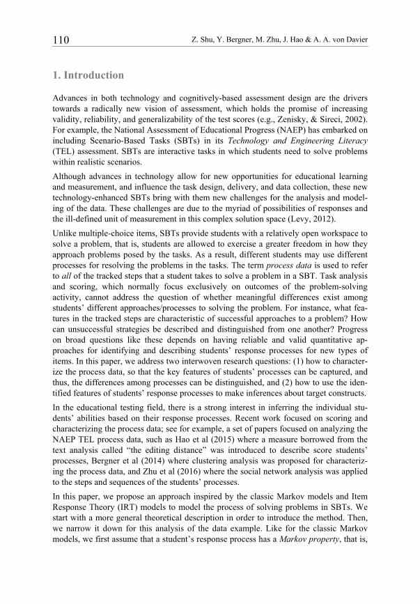
Eigenvalue decomposition and exploratory factor analysis were employed to evaluate dimensionality and determine the structure of the Q-matrix. The scree plot of the 18 eigenvalues is presented in Figure 2. Given the drop from 1.75 to .46 (from the second to third eigenvalues), the figure implies that there are two latent dimensions underlying the 18 variables. Given the exploratory purposes, an EFA with two latent factors was applied on the indicator matrix to explore the latent structure, and the latent structure was pro-posed based on a rule in which a variable was arbitrarily considered to be loaded on a factor when the absolute value of the loading was greater than 0.15. Note that a more adequate procedure would be the use of CFA instead of EFA and a target matrix of hy-
Figure 2:
Scree plot of eigenvalues of repeated actions as subcategories.
5 10 15
0.0
0.5
1.0
1.5
2.0
Number of Eigenvalues
Value
s
2.18
1.75
0.46
Z. Shu, Y. Bergner, M. Zhu, J. Hao & A. A. von Davier 122
pothetical loadings derived from the definition of concepts. However in this case, using the latent structure based on an EFA with an arbitrary cut point is mainly for demonstrat-ing the complete process of applying Markov-IRT.
Given the indicator matrix and the latent structured from the EFA analysis, the MIRT computer package (Haberman, 2013) was used to apply the two-dimensional GPCM model on the polytomous variables and the two-dimensional 2PL-IRT on the dichoto-mous variables. It converged after 177 cycles. Note, in an ideal case, the EFA and MIRT should be applied on different samples for a more robust analysis (e.g., split the sam-ples). However, the total number of students is about 1,300, which did not allow us to split the samples and apply the MIRT analysis on samples that are independent of the samples of the EFA analysis. As a compromise, we apply the MIRT and the EFA on the same data.
The general model-data fit, Penalty (as defined in Equation 5), was 0.512. The reliability of the first dimension is 0.90 and that of the second dimension is 0.91. The correlations between the two latent variables with the two TD scores are shown in Table 3. The first latent variable has a relatively strong positive correlation of 0.65 with the TD’s systema-ticity score, and the second one has a strong negative correlation -0.60 with TD’s effi-ciency score: the signs of these correlations correspond to the (dis)agreement of the action scoring and the definition of the scores, which is further discussed in a later sec-tion. It seems that the first latent variable reflects the systematicity of the processes, and the second one mirrors the efficiency of the processes. On one hand, the statistical results derived from a Markov-IRT analysis seem to support the definitions of systematicity and efficiency, and on the other hand, the two definitions could be used to verify and inter-pret the results derived from the model.
Table 3: Correlations between Latent Variables of Case I and TD scores
Score First latent variable Second latent variable
Efficiency Score -0.23 -0.60
Systematicity Score 0.65 -0.12
Case II: Repeated actions as new categories
In this case, the repeated actions/transitions were coded as new columns, the result for each student who selected the action was coded as 1; otherwise, it was coded as 0. Therefore, there were a total of 67 columns in the preliminary indicator matrix. A_t was used to label the repeated actions (A refers to the action, t refers to when the action A appears in the process). For example, some students selected the P action as many as 12 times, that is, there were 12 columns associated with the testing action. If a student only selected the testing action P 3 times, that student would be coded as 1 in the first three columns (i.e., P_1, P_2 and P_3 = 1) and 0 in the last 9 columns (i.e., P_4, P_5,…, and P_12 = 0). How-ever, there are 45 columns that had an average less than 0.1 and thus were excluded.
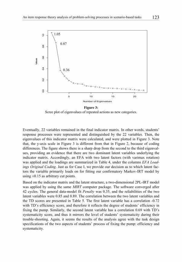
An item response theory analysis of problem-solving processes in scenario-based tasks 123
Figure 3:
Scree plot of eigenvalues of repeated actions as new categories.
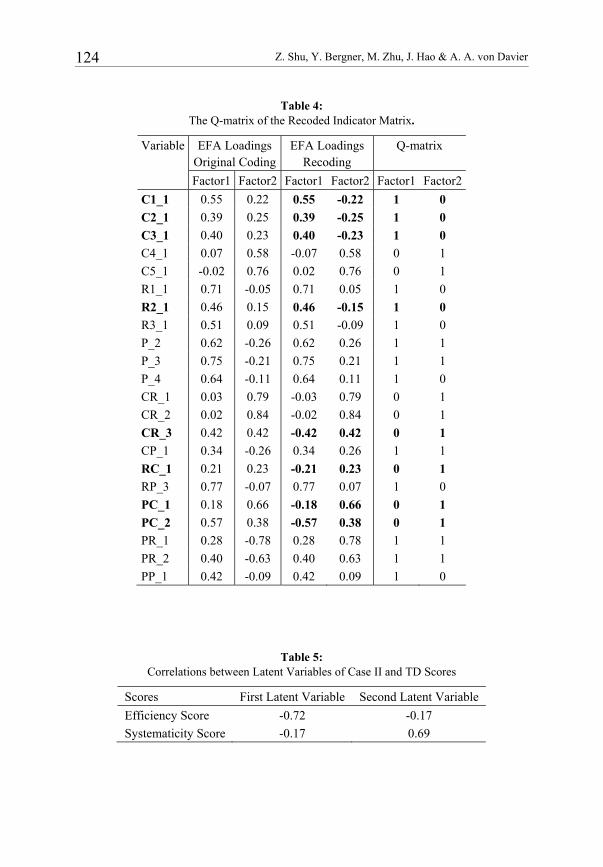
Eventually, 22 variables remained in the final indicator matrix. In other words, students’ response processes were represented and distinguished by the 22 variables. Then, the eigenvalues of this indicator matrix were calculated, and were plotted in Figure 3. Note that, the y-axis scale in Figure 3 is different from that in Figure 2, because of coding differences. The figure shows there is a sharp drop from the second to the third eigenval-ues, providing an evidence that there are two dominant latent variables underlying the indicator matrix. Accordingly, an EFA with two latent factors (with varimax rotation) was applied and the loadings are summarized in Table 4, under the columns EFA Load-ings Original Coding. Just as for Case I, we provide our decision as to which latent fac-tors the variable primarily loads on for fitting our confirmatory Markov-IRT model by using ±0.15 as arbitrary cut points.
Based on the indicator matrix and the latent structure, a two-dimensional 2PL-IRT model was applied by using the same MIRT computer package. The software converged after 42 cycles. The general data-model fit Penalty was 0.35, and the reliabilities of the two latent variables were 0.85 and 0.89. The correlation between the two latent variables and the TD scores are presented in Table 5. The first latent variable has a correlation -0.72 with TD’s efficiency score, and therefore it reflects the degree of students’ efficiency in fixing the pump. Similarly, the second latent variable has a correlation 0.69 with TD’s systematicity score, and thus it mirrors the level of students’ systematicity during their trouble-shooting. Again, it seems the results of the analysis agree with the task design specifications of the two aspects of students’ process of fixing the pump: efficiency and systematicity.
5 10 15 20
0.0
0.2
0.4
0.6
0.8
1.0
Number of Eigenvalues
Val
ues
1.05
0.87
0.36
Z. Shu, Y. Bergner, M. Zhu, J. Hao & A. A. von Davier 124
Table 4: The Q-matrix of the Recoded Indicator Matrix.
Variable EFA Loadings Original Coding
EFA Loadings Recoding
Q-matrix
Factor1 Factor2 Factor1 Factor2 Factor1 Factor2
C1_1 0.55 0.22 0.55 -0.22 1 0
C2_1 0.39 0.25 0.39 -0.25 1 0
C3_1 0.40 0.23 0.40 -0.23 1 0
C4_1 0.07 0.58 -0.07 0.58 0 1
C5_1 -0.02 0.76 0.02 0.76 0 1
R1_1 0.71 -0.05 0.71 0.05 1 0
R2_1 0.46 0.15 0.46 -0.15 1 0
R3_1 0.51 0.09 0.51 -0.09 1 0
P_2 0.62 -0.26 0.62 0.26 1 1
P_3 0.75 -0.21 0.75 0.21 1 1
P_4 0.64 -0.11 0.64 0.11 1 0
CR_1 0.03 0.79 -0.03 0.79 0 1
CR_2 0.02 0.84 -0.02 0.84 0 1
CR_3 0.42 0.42 -0.42 0.42 0 1
CP_1 0.34 -0.26 0.34 0.26 1 1
RC_1 0.21 0.23 -0.21 0.23 0 1
RP_3 0.77 -0.07 0.77 0.07 1 0
PC_1 0.18 0.66 -0.18 0.66 0 1
PC_2 0.57 0.38 -0.57 0.38 0 1
PR_1 0.28 -0.78 0.28 0.78 1 1
PR_2 0.40 -0.63 0.40 0.63 1 1
PP_1 0.42 -0.09 0.42 0.09 1 0
Table 5: Correlations between Latent Variables of Case II and TD Scores
Scores First Latent Variable Second Latent Variable
Efficiency Score -0.72 -0.17
Systematicity Score -0.17 0.69

An item response theory analysis of problem-solving processes in scenario-based tasks 125
Furthermore, there might be local dependence between the transitions and their corre-sponding actions. Therefore, we used generalized residuals (Bock & Haberman, 2009) to check the dependence. We did not observe significant generalized residuals indicating dependence among transitions and their actions. Furthermore, as indicated by the Q-matrix in Table 4, most of the transitions and their actions are loaded on two different dimensions, which also removes the concerns with the local dependence between the transitions and their corresponding actions.
Summary
Two types of indicator matrices were constructed with different treatments of the repeat-ed actions/transitions, where the Markov-IRT model with confirmatory latent structures was applied. As for the model-data fit index Penalty, Case II, for which the repeated actions/transitions were treated as new columns, was much better than Case I, for which repeated actions/transitions were treated as subcategories. With respect to the reliability of the latent variables, Case II was comparable to Case I. Moreover, Case II has a greater degree of agreement with the TD scores than Case I, and a greater level of correlation with the two TD scores. Therefore, we concluded that the Markov-IRT model based on the indicator matrix in Case II seems to be able to effectively characterize students’ response processes and capture the process features of interest, given its model-data fit and agreement with the ECD specifications.
4.2 Scoring under the ECD
The two latent variables of the Markov-IRT model, to a large degree, agree with the definition of the systematicity and efficiency specified in the task design. However, these two latent variables were derived through a pure data-driven analysis procedure, and as a result, they may not necessarily have all the properties of measurement scores. For ex-ample, the first latent variable strongly correlates with TD’s efficiency score, but nega-tively. In other words, the first latent variable is an opposite reflection of the construct, efficiency. Subsequently, a revision is necessary to align the model analysis results with the construct definitions and thus generate measurement scores that could correctly mir-ror the two constructs (i.e., efficiency and systematicity).
Furthermore, the efficiency in the Wells task refers to students only selecting the neces-sary actions and the systematicity is specified as following the correct order of steps. In the current indicator matrix, students’ selection of an action is coded as 1, if they select
Table 6: Correlations between Latent Variables of the Recoded Case II and TD Scores.
Score First Latent Variable Second Latent Variable
Efficiency Score 0.77 -0.28
Systematicity Score -0.07 0.64

Z. Shu, Y. Bergner, M. Zhu, J. Hao & A. A. von Davier 126
C1, C2, C3, R1, R2, and/or R3. Such coding is opposite to the definition of the efficiency score, and that is why the correlation between the first latent variable and the efficiency score is negative with a large absolute value. Therefore, the indicator matrix is recoded to be aligned with the ECD definition. As a result, the variables including C1_1, C2_1, C3_1, R1_1, R2_1, R3_1, P_2, P_3, P_4, CP_1, RP_3, PR_1, PR_2, PP_1 are reverse-coded; that is, 1 is recoded as 0, and 0 is recoded as 1. The EFA loadings with varimax rotation based on the recoded indicator matrix are shown in Table 4 under the columns EFA Loadings With Recoding. However, as indicted by Table 4 many variables have negative loadings on either one or both of the two factors. In order to increase the inter-pretability (i.e., a monotonic relationship between the latent scores and the number of actions taken), the variables with negative loadings are not loaded on the corresponding factor(s), and thus a Q-matrix, based on the recoded indicator matrix, is proposed as presented in Table 4 under the columns Q-matrix. Of the 22 variables, the 8 actions C1_1, C2_1, C3_1, R2_1, CR_3, RC_1, PC_1, PC_2 are now loaded on one single latent factor, not two as in the Case II application with original coding.
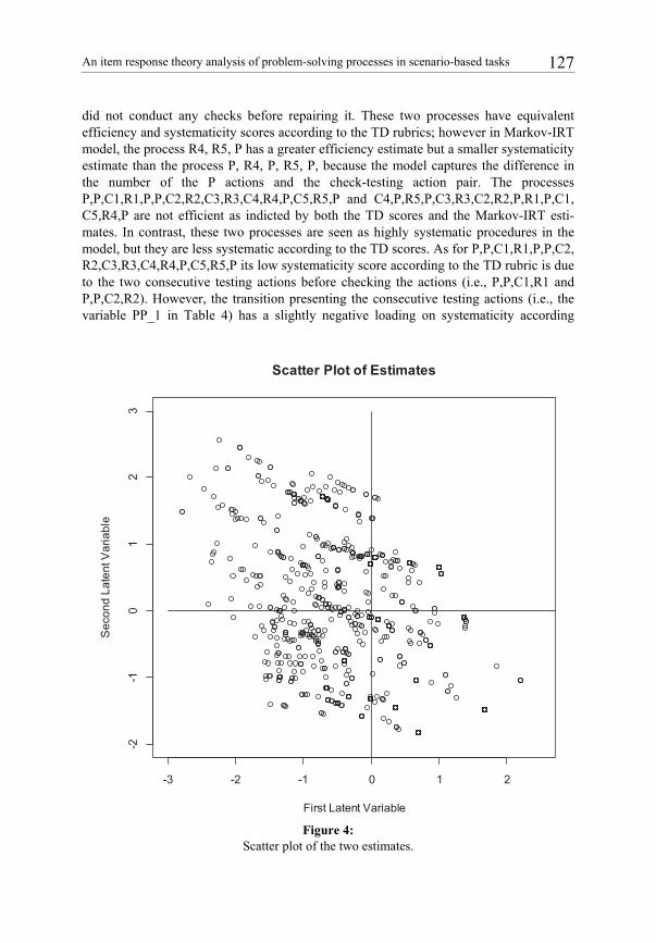
A two-dimensional 2PL-IRT was applied to the recoded matrix according to the Q-matrix. The software took 37 cycles to converge. The general model-data fit Penalty index was 0.37. The reliabilities of the latent variables were 0.84 and 0.89, respectively. Furthermore in Table 6, the correlation between the first latent variable and TD efficien-cy score is 0.77, and the correlation between the second latent variable and TD systema-ticity score is 0.64. The positive correlations indicate that the two latent variables, to a large degree, are in line with the ECD specifications (i.e., TD scores). A scatter plot (Figure 4) is provided to further demonstrate how the two dimensional estimates are distributed. The first latent variable has a range from -2.79 to 2.02, and the second one ranges from -1.82 to 2.56. In Table 7, four processes corresponding to maximum and minimum estimates are shown in Figure 4 and their TD scores are listed. Note, the num-ber of dots in Figure 4 is 427 not 1,318 (the total sample size), mainly because many students have used the same response processes. For example, there are 87 students using the response process sequence “R4,P,R5,P”.
In Table 7, the response processes P, R4,P,R5,P and R4, R5, P are seen as highly effi-cient but not systematic as indicated by both the TD scores and Markov-IRT estimates, because they only selected a minimum number of necessary actions to fix the pump but
Table 7: TD Scores of the Four Processes
Processes TD Efficiency
Score TD Systematic
Score
P,P,C1,R1,P,P,C2,R2,C3,R3,C4,R4,P,C5,R5,P 0 1
C4,P,R5,P,C3,R3,C2,R2,P,R1,P,C1,C5,R4,P 0 0
R4,P,R5,P 4 0
R4,R5,P 4 0
An item response theory analysis of problem-solving processes in scenario-based tasks 127
did not conduct any checks before repairing it. These two processes have equivalent efficiency and systematicity scores according to the TD rubrics; however in Markov-IRT model, the process R4, R5, P has a greater efficiency estimate but a smaller systematicity estimate than the process P, R4, P, R5, P, because the model captures the difference in the number of the P actions and the check-testing action pair. The processes P,P,C1,R1,P,P,C2,R2,C3,R3,C4,R4,P,C5,R5,P and C4,P,R5,P,C3,R3,C2,R2,P,R1,P,C1, C5,R4,P are not efficient as indicted by both the TD scores and the Markov-IRT esti-mates. In contrast, these two processes are seen as highly systematic procedures in the model, but they are less systematic according to the TD scores. As for P,P,C1,R1,P,P,C2, R2,C3,R3,C4,R4,P,C5,R5,P its low systematicity score according to the TD rubric is due to the two consecutive testing actions before checking the actions (i.e., P,P,C1,R1 and P,P,C2,R2). However, the transition presenting the consecutive testing actions (i.e., the variable PP_1 in Table 4) has a slightly negative loading on systematicity according
Figure 4:
Scatter plot of the two estimates.
-3 -2 -1 0 1 2
-2-1
01
23
Scatter Plot of Estimates
First Latent Variable
elbairaV tnetaL dnoce
S

Z. Shu, Y. Bergner, M. Zhu, J. Hao & A. A. von Davier 128
to the factor analysis, and thus is not treated as an indicator of the systematicity in the Markov-IRT model. As a result, the systematicity of the process is not penalized by the Markov-IRT model and was assigned with a high systematicity score. As for C4,P,R5,P,C3,R3,C2,R2,P,R1,P,C1,C5,R4,P it has the lowest systematicity score accord-ing to the TD scoring rubrics, because the student transits from one checking action to a not-associated repair action. In contrast, this process is seen as a systematic procedure in the Markov-IRT model, because it has the features of being systematically derived from the factor analysis defined in Table 4. Such difference between the TD scores and the Markov-IRT estimates explains why the correlations between the TD scores and the estimates are between 0.6 and 0.8. Furthermore, there are a total of 543 unique response processes among the 1,318 students and a total of 427 dots in Figure 4. In other words, the two estimates of the Markov-IRT model could distinguish 427 out of 543 unique response processes. Among those patterns that are not distinguished, many are highly similar to each other, such as “R5,P,R4,P” and ”R4,P,R5,P”.
5. Discussion
Although SBTs have great potential in terms of increasing test validity of the test scores and offering the opportunity of including cognitive-based learning tasks into the assess-ment, a critical component is having rigorous methods for analyzing and interpreting data collected with these tasks. The sheer abundance and varied formats of data collected by SBTs are aspects that we have not previously encountered in traditional paper-pencil assessments, as such this data poses several challenges for analysis, interpretation, and reporting. In this paper, the Markov-IRT model is proposed to characterize the process data consisting of a finite space of actions, collected via the new item types (e.g., SBTs).
The proposed method seems to be a useful tool to capture the process features of interest in the case study. However, it has limitations. First, this model requires fairly strong assumptions that a student’s response process has a Markov property and the latent trait(s) are normally distributed. In particular, the Markov assumption constrains the dependency among actions/states of a process within two consecutive time points, and therefore, the model does not model action-sequence along all the time points. Second, factor analysis is proposed to evaluate the dimensionality and the latent structure of the indicator matrix, which requires some arbitrary decisions and/or demands inputs from item developers and cognitive scientists. In this real data application, a simplified factor analysis was used for demonstration purposes, however, a more complete process could be used for a more reliable decision of the latent structure of the indicator matrix. For example, an arbitrary cut point was selected to determine the latent structure in the real application. However, in a more robust analysis procedure, EFA analyses with different rotation methods should be used for exploring different loadings patterns. Then, CFA analyses with split samples should be employed to further evaluate and compare the model-data fit of different latent structures for a more robust selection of the latent struc-ture. Last, how to use the scores derived from the Markov-IRT model is discussed in the application example. However, in other settings, the score from the model may be differ-ent and specific to its design.
An item response theory analysis of problem-solving processes in scenario-based tasks 129
Acknowledgements
This research has been greatly improved upon by valuable suggestions from ETS internal review. We would like to express our sincere gratitude to Drs. Shelby Haberman and Katherine Castellano for their comments on the previous version of this paper. We also want to acknowledge the editorial help of Mrs. Laura Frisby from ACTNext, by ACT. This work was conducted while Yoav Berner and Alina A. von Davier were employed with Eucational Testing Service. The opinions presented here are those of the authors and do not reflect the opinions of ETS or ACT.
References
Almond, R.G., Steinberg, L.S., & Mislevy, R.J. (1999). A sample assessment using the four process framework. White paper prepared for the IMS Inter-Operability Standards Working Group. Princeton, NJ: Educational Testing Service
Baum, L. E., & Petrie, T. (1966). Statistical inference for probabilistic functions of finite state Markov chains. The Annals of Mathematical Statistics, 37, 1554–1563.
Bellman, R., (1957). A Markovian decision process. Journal of Mathematics and Mechanics, 4, 66-77.
Bergner, Y., Shu, Z., von Davier, A. (2014). Visualization and Confirmatory Clustering of Sequence Data from a Simulation-Based Assessment Task. Proceedings of the 7th International Conference on Educational Data Mining (EDM). 2014.
Bock, R. D. (1972). Estimating item parameters and latent ability when responses are scored in two or more nominal categories. Psychometrika, 37, 29-51.
Bock, R. D., & Haberman, S. J. (2009, July). Confidence bands for examining goodness-of-fit of estimated item response functions. Paper presented at the annual meeting of the Psychometric Society, Cambridge, UK.
Bush, R. R., & Mosteller, F. (1951). A mathematical model for simple learning. Psychological Review, 58, 313-323.
Estes, W. K. (1950). Toward a statistical theory for learning. Psychological review, 57, 94-107.
Gilula, Z., & Haberman, S. J. (2001). Analysis of categorical response profiles by informative summaries. Sociological Methodology, 31, 129–187.
Haberman, S. J. (2006). An elementary test of the normal 2PL model against the normal 3PL alternative (Research Report RR-06-14). Princeton, NJ: Educational Testing Service.
Haberman, S. J. (2009). Use of generalized residuals to examine goodness of fit of item response models (ETS Research Report No. RR-09-15). Princeton, NJ: ETS.
Haberman, S. J. (2013). A general program for item-response analysis that employs the stabilized Newton-Raphson algorithm. Princeton, NJ: Educational Testing Service.
Hambleton, R.K., & Swaminathan, H. (1985). Item response theory, principles and applications. MA: Kluwer Academic Publisher.
Hao, J., Shu, Z., von Davier, A. (2014). Analyzing Process Data from Game/Scenario-Based Tasks: An Edit Distance Approach. Journal of Educational Data Mining, 7(1), pp.33-50
Kemeny, J. G., & Snell, J. L.(1957). Markov process in the learning theory. Psychometrika, 22, 221-230.

Z. Shu, Y. Bergner, M. Zhu, J. Hao & A. A. von Davier 130
Levy, R. (2012). Psychometric advances, opportunities, and challenges for simulation-based Assessment. Paper presented at Invitational Research Symposium on Technology Enhanced Assessments. National Harbor, MD.
Markov, A. A. (1971). Extension of the limit theorems of probability theory to a sum of variables connected in a chain. Reprinted in Appendix B of: R. Howard. Dynamic Probabilistic Systems, volume 1: Markov Chains. New York, NY: Wiley.
Muraki, E. (1992). A generalized partial credit model: Application of an EM algorithm. Applied Psychological Measurement, 16, 159-176.
Puterman, M. (1994). Markov decision processes. New York, NY: Wiley. Rabiner, L. R. (1989). A tutorial on hidden Markov models and selected applications in
speech recognition. In Proceedings of the Institute of Electrical and Electronics Engineers, 257–286.
Rabiner, L. R., Lee, C. H., Juang, B. H., & Wilpon, J. G., (1989). HMM clustering for connected word recognition. In Proceedings of the Institute of Electrical and Electronics Engineers ICASSP, 405-408.
Savage, L. J. (1971). Elicitation of personal probabilities and expectations. Journal of the American Statistical Association, 66, 783–801.
Seneta, E. (1996). Markov and the birth of chain dependence theory. International Statistical Review 64, 255–263.
Shih, B., Koedinger, K. R., & Scheines, R., (2010). Discovery of learning tactics using hidden Markov model clustering. In proceedings of the 3rd International Conference on Educational Data Mining, Montreal, Canada.
Tatsuoka, K. K.(1983). Rule space: a method for dealing with misconception based on item response theory. Journal of Educational Measurement, 20(4), pp.345-354.
van de Pol, F., & Langeheine, R. (1990). Mixed Markov latent class models. In, C. C. Clogg (Ed.) Sociological Methodology 1990 (pp. 213-24). Oxford, England: Blackwell.
Zenisky, A. L., & Sireci, S. G. (2002). Technological innovations in large-scale assessment. Applied Measurement in Education, 15, 337-362.
Zhu, M., Shu, Z., & von Davier, A. A. (2016). Using Networks to Visualize and Analyze Process Data for Educational Assessment. Journal of Educational Measurement, 53(2), 190–211.
Appendix A
Efficiency scoring rubric:
The following are general guidelines used to define "efficiency" as used in the scoring rules.
* The pump is exhibiting problems 4 & 5 (addressed by C4, R4, C5, R5). Students should not perform any check or repair actions related to problems which are not exhib-ited.
* Performing an unnecessary repair is penalized more than performing an unnecessary check, as this is a more inefficient procedure.
Efficient actions - E = {P, C4, R4, C5, R5}

An item response theory analysis of problem-solving processes in scenario-based tasks 131
Unnecessary checks - C = {C1, C2, C3}
Unnecessary repairs - R = {R1, R2, R3}
4 - Only actions from set E
3 - Actions from E + 1 action from C
2A - Actions from E + 2-3 actions from C
2B - Actions from E + 0-1 action from C + 1 action from R
1 - Actions from E + 2-3 actions from C + 1-2 actions from R
0 - Actions from E + 3 actions from C + 3 actions from R
Systematic scoring rubric:
The following are general guidelines used to define sequences used in the scoring rules.
* Students should not perform a repair before checking to verify that the repair they are performing will address the symptom they are attempting to address with the repair.
* Once a student has performed a repair, that student should check to see if the problem is solved by trying out the pump (action P). Any additional Ps are irrelevant and will be ignored for scoring purposes.
* Students who use a very inefficient procedure for repairing the pump will receive a low score for systematicity, as students who are performing a lot of unnecessary steps may be following a systematic procedure unrelated to troubleshooting/repair (e.g. pushing all buttons on the interface is in some sense "systematic" but does not provide meaningful evidence of troubleshooting/repair skill).
3 - All checks performed before repairs; pump is checked immediately following each repair
2 - All checks performed before repairs; pump is not checked immediately following each repair
1 - One repair is performed before the associated check (or check is omitted); pump may not be checked immediately following each repair
0 - Two or more repairs performed before the associated check; pump may not be checked immediately following each repair.


![[IRT] Item Response Theory Reference Manual](https://static.fdocuments.net/doc/165x107/5879ee1c1a28ab82408bc4f0/irt-item-response-theory-reference-manual.jpg)

![[IRT] Item Response Theory - Survey Design](https://static.fdocuments.net/doc/165x107/6215d6629ffc9d5ad40f105b/irt-item-response-theory-survey-design.jpg)