An Invitation to Sample Paths of Brownian Motionperes/bmall.pdf · An Invitation to Sample Paths of...
68
An Invitation to Sample Paths of Brownian Motion Yuval Peres Lecture notes edited by B´ alint Vir´ ag, Elchanan Mossel and Yimin Xiao Version of November 1, 2001 1
Transcript of An Invitation to Sample Paths of Brownian Motionperes/bmall.pdf · An Invitation to Sample Paths of...

An Invitation to SamplePaths of Brownian Motion
Yuval Peres
Lecture notes edited by Balint Virag, Elchanan Mossel and Yimin Xiao
Version of November 1, 2001
1

2
Preface. These notes record lectures I gave at the Statistics Department, University ofCalifornia, Berkeley in Spring 1998. I am grateful to the students who attended the courseand wrote the first draft of the notes: Diego Garcia, Yoram Gat, Diogo A. Gomes, CharlesHolton, Frederic Latremoliere, Wei Li, Ben Morris, Jason Schweinsberg, Balint Virag, YeXia and Xiaowen Zhou. The draft was edited by Balint Virag, Elchanan Mossel, SerbanNacu and Yimin Xiao. I thank Pertti Mattila for the invitation to lecture on this materialat the joint summer school in Jyvaskyla, August 1999.

Contents
Chapter 1. Brownian Motion 11. Motivation – Intersection of Brownian paths 12. Gaussian random variables 13. Levy’s construction of Brownian motion 44. Basic properties of Brownian motion 65. Hausdorff dimension and Minkowski dimension 116. Hausdorff dimension of the Brownian path and the Brownian graph 137. On nowhere differentiability 178. Strong Markov property and the reflection principle 189. Local extrema of Brownian motion 2010. Area of planar Brownian motion paths 2011. Zeros of the Brownian motion 2212. Harris’ Inequality and its consequences 2713. Points of increase for random walks and Brownian motion 2914. Frostman’s Lemma, energy, and dimension doubling 3315. Skorokhod’s representation 3916. Donsker’s Invariance Principle 4317. Harmonic functions and Brownian motion in R
d 4718. Maximum principle for harmonic functions 5019. The Dirichlet problem 5120. Polar points and recurrence 5221. Capacity and harmonic functions 5422. Kaufman’s theorem on uniform dimension doubling 5723. Packing dimension 5924. Hausdorff dimension and random sets 6025. An extension of Levy’s modulus of continuity 61References 63
3

CHAPTER 1
Brownian Motion
1. Motivation – Intersection of Brownian paths
Consider a number of Brownian motion paths started at different points. Say that theyintersect if there is a point which lies on all of the paths. Do the paths intersect? Theanswer to this question depends on the dimension:
• In R2, any finite number of paths intersect with positive probability (this is atheorem of Dvoretsky, Erdos, Kakutani in the 1950’s),
• In R3, two paths intersect with positive probability, but not three (this is a theoremof Dvoretsky, Erdos, Kakutani and Taylor, 1957),
• In Rd for d ≥ 4, no pair of paths intersect with positive probability.The principle we will use to establish these results is intersection equivalence between
Brownian motion and certain random Cantor-type sets. Here we will introduce the conceptfor R
3 only. Partition the cube [0, 1]3 in eight congruent sub-cubes, and keep each of thesub-cubes with probability 1
2 . For each cube that remained at the end of this stage, partitionit into eight sub-cubes, keeping each of them with probability 1
2 , and so on. Let Q(3, 1
2
)denote the limiting set— that is, the intersection of the cubes remaining at all steps. Thisset is not empty with positive probability, since, if we consider that the remaining sub-cubes of a given cube as its “children” in a branching process, then the expected numberof offsprings is four, so this process has positive probability not to die out.
One can prove that, there exist two positive constants C1, C2 such that, if Λ is a closedsubset of [0, 1]3, and Bt is a Brownian motion started at a point uniformly chosen in[0, 1]3, then:
C1P(Q
(3,
12
)∩ Λ 6= ∅
)≤ P (∃t ≥ 0 Bt ∈ Λ) ≤ C2P
(Q
(3,
12
)∩ Λ 6= ∅
)The motivation is that, though the intersection of two independent Brownian paths is
a complicated object, the intersection of two sets of the form Q(3, 1
2
)is a set of the same
kind—namely, Q(3, 1
4
). The previously described branching process dies out as soon as we
intersect more than two of these Cantor-type sets—hence the result about intersection ofpaths in R
3.
2. Gaussian random variables
Brownian motion is at the meeting point of the most important categories of stochasticprocesses: it is a martingale, a strong Markov process, a process with independent andstationary increments, and a Gaussian process. We will construct Brownian motion as aspecific Gaussian process. We start with the definitions of Gaussian random variables:
1

2 1. BROWNIAN MOTION
Definition 2.1. A real-valued random variable X on a probability space (Ω,F ,P) hasa standard Gaussian (or standard normal) distribution if
P(X > x) =1√2π
∫ +∞
xe−u
2/2du
A vector-valued random variable X has an n-dimensional standard Gaussian dis-tribution if its n coordinates are standard Gaussian and independent.
A vector-valued random variable Y : Ω → Rp is Gaussian if there exists a vector-valued random variable X having an n-dimensional standard Gaussian distribution, a p×nmatrix A and a p-dimensional vector b such that:
Y = AX + b (2.1)
We are now ready to define the Gaussian processes.
Definition 2.2. A stochastic process (Xt)t∈I is said to be a Gaussian process if forall k and t1, . . . , tk ∈ I the vector (Xt1, . . . , Xtk)
t is Gaussian.
Recall that the covariance matrix of a random vector is defined as
Cov(Y ) = E[(Y − EY )(Y − EY )t
]Then, by the linearity of expectation, the Gaussian vector Y in (2.1) has
Cov(Y ) = AAt.
Recall that an n×n matrix A is said to be orthogonal if AAt = In. The following lemmashows that the distribution of a Gaussian vector is determined by its mean and covariance.
Lemma 2.3.(i) If Θ is an orthogonal n × n matrix and X is an n-dimensional standard Gaussian
vector, then ΘX is also an n-dimensional standard Gaussian vector.(ii) If Y and Z are Gaussian vectors in R
n such that EY = EZ and Cov(Y ) = Cov(Z),then Y and Z have the same distribution.
Proof.
(i) As the coordinates of X are independent standard Gaussian, X has density givenby:
f(x) = (2π)−n2 e−‖x‖2/2
where ‖ · ‖ denotes the Euclidean norm. Since Θ preserves this norm, the density of X isinvariant under Θ.
(ii) It is sufficient to consider the case when EY = EZ = 0. Then, using Definition 2.1,there exist standard Gaussian vectors X1, X2 and matrices A,C so that
Y = AX1 and Z = CX2.
By adding some columns of zeroes to A or C if necessary, we can assume that X1, X2 areboth k-vectors for some k and A, C are both n× k matrices.
Let A, C denote the vector spaces generated by the row vectors of A and C, respectively.To simplify notations, assume without loss of generality that the first ` row vectors of A
2. GAUSSIAN RANDOM VARIABLES 3
form a basis for the space A. For any matrix M let Mi denote the ith row vector of M ,and define the linear map Θ from A to C by
AiΘ = Ci for i = 1, . . . , `.
We want to check that Θ is an isomorphism. Assume that there is a vector v1A1+ · · ·+v`A`whose image is 0. Then the k-vector v = (v1, v2, . . . , v`, 0, . . . , 0) satisfies vtC = 0, and so‖vtA‖2 = vtAAtv = vtCCtv = 0, giving vtA = 0. This shows that Θ is one-to-one, inparticular dimA ≤ dim C. By symmetry A and C must have the same dimension, so Θ isan isomorphism.
As the coefficient (i, j) of the matrixAAt is the scalar product of Ai and Aj, the identityAAt = CCt implies that Θ is an orthogonal transformation from A to C. We can extendit to map the orthocomplement of A to the orthocomplement of C orthogonally, getting anorthogonal map Θ : R
k → Rk. Then
Y = AX1, Z = CX2 = AΘX2,
and (ii) follows from (i).
Thus, the first two moments of a Gaussian vector are sufficient to characterize its distri-bution, hence the introduction of the notation N (µ,Σ) to designate the normal distributionwith expectation µ and covariance matrix Σ. A useful corollary of this lemma is:
Corollary 2.4. Let Z1, Z2 be independent N (0, σ2) random variables. Then Z1 + Z2
and Z1 −Z2 are two independent random variables having the same distribution N (0, 2σ2).
Proof. σ−1(Z1, Z2) is a standard Gaussian vector, and so, if:
Θ =1√2
[1 11 −1
]then Θ is an orthogonal matrix such that
(√
2σ)−1(Z1 + Z2, Z1 − Z2)t = Θσ−1(Z1, Z2)t,
and our claim follows from part (i) of the Lemma.
As a conclusion of this section, we state the following tail estimate for the standardGaussian distribution:
Lemma 2.5. Let Z be distributed as N (0, 1). Then for all x ≥ 0:
x
x2 + 11√2πe−x
2/2 ≤ P (Z > x) ≤ 1x
1√2πe−x
2/2
Proof. The right inequality is obtained by the estimate:
P(Z > x) ≤∫ +∞
x
u
x
1√2πe−u
2/2du
since, in the integral, u ≥ x. The left inequality is proved as follows: Let us define
f(x) := xe−x2/2 − (x2 + 1)
∫ +∞
xe−u
2/2du
4 1. BROWNIAN MOTION
We remark that f(0) < 0 and limx→+∞ f(x) = 0. Moreover,
f ′(x) = (1− x2 + x2 + 1)e−x2/2 − 2x
∫ +∞
x
e−u2/2du
= −2x(∫ +∞
xe−u
2/2du− 1xe−x
2/2
),
so the right inequality implies f ′(x) ≥ 0 for all x ≥ 0. This implies f(x) ≤ 0, proving thelemma.
3. Levy’s construction of Brownian motion
3.1. Definition. Standard Brownian motion on an interval I = [0, a] or I = [0,∞) isdefined by the following properties:
Definition 3.1. A real-valued stochastic process Btt∈I is a standard Brownianmotion if it is a Gaussian process such that:
(i) B0 = 0,(ii) ∀k natural and ∀t1 < . . . < tk in I : Btk −Btk−1
, . . . , Bt2 −Bt1 are independent,(iii) ∀t, s ∈ I with t < s Bs −Bt has N (0, s− t) distribution.(iv) Almost surely, t 7→ Bt is continuous on I .
As a corollary of this definition, one can already remark that for all t, s ∈ I :
Cov(Bt, Bs) = s ∧ t.Indeed, assume that t ≥ s. Then Cov(Bt, Bs) = Cov(Bt − Bs, Bs) + Cov(Bs, Bs) bybilinearity of the covariance. The first term vanishes by the independence of increments,and the second term equals s by properties (iii) and (i). Thus by Lemma 2.3 we may replaceproperties (ii) and (iii) in the definition by:
• For all t, s ∈ I , Cov(Bt, Bs) = t ∧ s.• For all t ∈ I , Bt has N (0, t) distribution.
or by:• For all t, s ∈ I with t < s, Bt − Bs and Bs are independent.• For all t ∈ I , Bt has N (0, t) distribution.
Kolmogorov’s extension theorem implies the existence of any countable time set sto-chastic process Xt if we know its finite-dimensional distributions and they are consistent.Thus, standard Brownian motion could be easily constructed on any countable time set.However knowing finite dimensional distributions is not sufficient to get continuous paths,as the following example shows.
Example 3.2. Suppose that standard Brownian motion Bt on [0, 1] has been con-structed, and consider an independent random variable U uniformly distributed on [0, 1].Define:
Bt =Bt if t 6= U0 otherwise
The finite-dimensional distributions of Bt are the same as the ones of Bt. However, theprocess Bt has almost surely discontinuous paths.

3. LEVY’S CONSTRUCTION OF BROWNIAN MOTION 5
In measure theory, one often identifies functions with their equivalence class for almost-everywhere equality. As the above example shows, it is important not to make this iden-tification in the study of continuous-time stochastic processes. Here we want to define aprobability measure on the set of continuous functions.
3.2. Construction. The following construction, due to Paul Levy, consist of choosingthe “right” values for the Brownian motion at each dyadic point of [0, 1] and then inter-polating linearly between these values. This construction is inductive, and, at each step,a process is constructed, that has continuous paths. Brownian motion is then the uniformlimit of these processes—hence its continuity. We will use the following basic lemma. Theproof can be found, for instance, in Durrett (1995).
Lemma 3.3 (Borel-Cantelli). Let Aii=0,...,∞ be a sequence of events, and let
Ai i.o. = lim supi→∞
Ai =∞⋂i=0
∞⋃j=i
Aj ,
where “i.o.” abbreviates “infinitely often”.(i) If
∑∞i=0 P(Ai) <∞, then P(Ai i.o.) = 0.
(ii) If Ai are pairwise independent, and∑∞
i=0 P(Ai) = ∞, then P(Ai i.o.) = 1.
Theorem 3.4 (Wiener 1923). Standard Brownian motion on [0,∞) exists.
Proof. (Levy 1948)We first construct standard Brownian motion on [0, 1]. For n ≥ 0, let Dn = k/2n : 0 ≤
k ≤ 2n, and let D =⋃Dn. Let Zdd∈D be a collection of independent N (0, 1) random
variables. We will first construct the values of B on D. Set B0 = 0, and B1 = Z1. In aninductive construction, for each n we will construct Bd for all d ∈ Dn so that
(i) For all r < s < t in Dn, the increment Bt −Bs has N (0, t− s) distribution andis independent of Bs − Br.
(ii) Bd for d ∈ Dn are globally independent of the Zd for d ∈ D \Dn.
These assertions hold for n = 0. Suppose that they hold for n − 1. Define, for alld ∈ Dn \Dn−1, a random variable Bd by
Bd =Bd− +Bd+
2+
Zd
2(n+1)/2(3.1)
where d+ = d + 2−n, and d− = d − 2−n, and both are in Dn−1. Since 12 [Bd+ − Bd− ] is
N (0, 1/2n+1) by induction, and Zd/2(n+1)/2 is an independent N (0, 1/2n+1), their sum andtheir difference, Bd−Bd− and Bd+−Bd are both N (0, 1/2n) and independent by Corollary2.4. Assertion (i) follows from this and the inductive hypothesis, and (ii) is clear.
Having thus chosen the values of the process on D, we now “interpolate” between them.Formally, let F0(x) = xZ1, and for n ≥ 1, let let us introduce the function:
Fn(x) =
2−(n+1)/2Zx for x ∈ Dn \Dn−1,0 for x ∈ Dn−1,linear between consecutive points in Dn.
(3.2)

6 1. BROWNIAN MOTION
These functions are continuous on [0, 1], and for all n and d ∈ Dn
Bd =n∑i=0
Fi(d) =∞∑i=0
Fi(d). (3.3)
This can be seen by induction. Suppose that it holds for n− 1. Let d ∈ Dn −Dn−1. Sincefor 0 ≤ i ≤ n − 1 Fi is linear on [d−, d+], we get
n−1∑i=0
Fi(d) =n−1∑i=1
Fi(d−) + Fi(d+)2
=Bd− +Bd+
2. (3.4)
Since Fn(d) = 2−(n+1)/2Zd, comparing (3.1) and (3.4) gives (3.3).On the other hand, we have, by definition of Zd and by Lemma 2.5:
P(|Zd| ≥ c
√n) ≤ exp
(−c
2n
2
)for n large enough, so the series
∑∞n=0
∑d∈Dn
P(|Zd| ≥ c√n) converges as soon as c >√
2 log2. Fix such a c. By the Borel-Cantelli Lemma 3.3 we conclude that there exists arandom but finite N so that for all n > N and d ∈ Dn we have |Zd| < c
√n, and so:
‖Fn‖∞ < c√n2−n/2. (3.5)
This upper bound implies that the series∑∞
n=0 Fn(t) is uniformly convergent on [0, 1],and so it has a continuous limit, which we call Bt. All we have to check is that theincrements of this process have the right finite-dimensional joint distributions. This is adirect consequence of the density of the set D in [0, 1] and the continuity of paths. Indeed,let t1 > t2 > t3 be in [0, 1], then they are limits of sequences t1,n, t2,n and t3,n in D,respectively. Now
Bt3 −Bt2 = limk→∞
(Bt3,k−Bt2,k
)
is a limit of Gaussian random variables, so itself is Gaussian with mean 0 and vari-ance limn→∞ (t3,n − t2,n) = t3 − t2. The same holds for Bt2 − Bt1, moreover, these tworandom variables are limit of independent random variables, since for n large enough,t1,n > t2,n > t3,n. Applying this argument for any number of increments, we get thatBt has independent increments such that and for all s < t in [0, 1] Bt−Bs has N (0, t−s)distribution.
We have thus constructed Brownian motion on [0, 1]. To conclude, if Bnt t for n ≥ 0are independent Brownian motions on [0, 1], then
Bt = Bbtct−btc +
∑0≤i<btc
Bi1
meets our definition of Brownian motion on [0,∞).
4. Basic properties of Brownian motion
Let B(t)t≥0 be a standard Brownian motion, and let a 6= 0. The following scalingrelation is a simple consequence of the definitions.
1aB(a2t)t≥0
d= B(t)t≥0.

4. BASIC PROPERTIES OF BROWNIAN MOTION 7
Also, define the time inversion of Bt as
W (t) =
0 t = 0;tB( 1
t ) t > 0.
We claim that W is a standard Brownian motion. Indeed,
Cov(W (t), W (s)) = tsCov(B(1t,1s)) = ts (
1t∧ 1s) = t ∧ s,
so W and B have the same finite dimensional distributions, and they have the same dis-tributions as processes on the rational numbers. Since the paths of W (t) are continuousexcept maybe at 0, we have
limt↓0
W (t) = limt↓0,t∈Q
W (t) = 0 a.s.
so the paths of W (t) are continuous on [0,∞) a.s. As a corollary, we get
Corollary 4.1. [Law of Large Numbers for Brownian motion]
limt→∞
B(t)t
= 0 a.s.
Proof. limt→∞B(t)t = limt→∞W ( 1
t ) = 0 a.s.
Exercise 4.2. Prove this result directly. Use the usual Law of Large Numbers to showthat limn→∞
B(n)n = 0. Then show that B(t) does not oscillate too much between n and
n+ 1.
Remark. The symmetry inherent in the time inversion property becomes more appar-ent if one considers the Ornstein-Uhlenbeck diffusion, which is given by
X(t) = e−tB(e2t)
This is a stationary Markov chain with X(t) ∼ N (0, 1) for all t. It is a diffusion witha drift toward the origin proportional to the distance from the origin. Unlike Brownianmotion, the Ornstein-Uhlenbeck diffusion is time reversible. The time inversion formulagives X(t)t≥0
d= X(−t)t≥0. For t near −∞, X(t) relates to the Brownian motion near0, and for t near ∞, X(t) relates to the Brownian motion near ∞.
One of the advantages of Levy’s construction of Brownian motion is that it easily yieldsa modulus of continuity result. Following Levy, we defined Brownian motion as an infinitesum
∑∞n=0 Fn, where each Fn is a piecewise linear function given in (3.2). Its derivative
exists almost everywhere, and by definition and (3.5)
‖F ′n‖∞ ≤ ‖Fn‖∞
2−n≤ C1(ω) +
√n 2n/2 (4.1)
The random constant C1(ω) is introduced to deal with the finitely many exceptions to (3.5).Now for t, t+ h ∈ [0, 1], we have
|B(t+ h) −B(t)| ≤∑n
|Fn(t+ h) − Fn(t)| ≤∑n≤`
h‖F ′n‖∞ +
∑n>`
2‖Fn‖∞ (4.2)

8 1. BROWNIAN MOTION
By (3.5) and (4.1) if ` > N for a random N , then the above is bounded by
h(C1(ω) +∑n≤`
c√n 2n/2) + 2
∑n>`
c√n 2−n/2
≤ C2(ω)h√` 2`/2 + C3(ω)
√` 2−`/2
The inequality holds because each series is bounded by a constant times its dominant term.Choosing ` = blog2(1/h)c, and choosing C(ω) to take care of the cases when ` ≤ N , we get
|B(t+ h) − B(t)| ≤ C(ω)
√h log2
1h. (4.3)
The result is a (weak) form of Levy’s modulus of continuity. This is not enough to makeBt a differentiable function since
√h h for small h. But we still have
Corollary 4.3. For every α < 12 , Brownian paths are α - Holder a.s.
Exercise 4.4. Show that a Brownian motion is a.s. not 12 - Holder.
Remark. There does exist a t = t(ω) such that |B(t+h)−B(t)| ≤ C(ω)h12 for every h,
a.s. However, such t have measure 0. This is the slowest movement that is locally possible.
Solution. Let Ak,n be the event that B((k + 1)2−n) − B(k2−n) > c√
n2−n/2. Then Lemma 2.5implies
P(Ak,n) = P(B(1) > c√
n) ≥ c√
n
c2n + 1e−c2n/2.
If 0 < c <√
2 log(2) then c2/2 < log(2) and 2nP(Ak,n) → ∞. Therefore,
P(2n⋂
k=1
Ack,n) = [1 − P(Ak,n)]2
n ≤ e−2nP(Ak,n) → 0 as n → ∞.
The last inequality comes from the fact that 1 − x ≤ e−x for all x. By considering h = 2−n, onecan see that
P(∀h B(t + h) − B(t) ≤ c
√h log2 h−1
)= 0 if c <
√2 log 2.
We remark that the paths are a.s. not 12-Holder. Indeed, the log2(
1h) factor in (4.3) cannot be
ignored. We will see later that the Hausdorff dimension of the graph of Brownian motion is 32 a.s.
Having proven that Brownian paths are somewhat “regular”, let us see why they are“bizarre”. One reason is that the paths of Brownian motion have no intervals of mono-tonicity. Indeed, if [a, b] is an interval of monotonicity, then dividing it up into n equalsub-intervals [ai, ai+1] each increment B(ai)−B(ai+1) has to have the same sign. This hasprobability 2 · 2−n, and taking n → ∞ shows that the probability that [a, b] is an intervalof monotonicity must be 0. Taking a countable union gives that there is no interval ofmonotonicity with rational endpoints, but each monotone interval would have a monotonerational sub-interval.
We will now show that for any time t0, Brownian motion is not differentiable at t0. Forthis, we need a simple proposition.
Proposition 4.5. A.s.
lim supn→∞
B(n)√n
= +∞, lim infn→∞
B(n)√n
= −∞. (4.4)

4. BASIC PROPERTIES OF BROWNIAN MOTION 9
Remark. Comparing this with Corollary 4.1, it is natural to ask what sequence B(n)should be divided by to get a lim sup which is greater than 0 but less than ∞. An answeris given by the law of the iterated logarithm in a later section.
The proof of (4.4) relies on the following standard fact, whose proof can be found, forexample, in Durrett (1995). Consider a probability measure on the space of real sequences,and let X1, X2, . . . be the sequence of random variables it defines. An event, that is a mea-surable set of sequences, A is exchangeable if X1, X2, . . . satisfy A implies that Xσ1, Xσ2, . . .satisfy A for all finite permutations σ. Here finite permutation means that σn = n for allsufficiently large n.
Proposition 4.6 (Hewitt-Savage 0-1 Law). If A is an exchangeable event for an i.i.d.sequence then P(A) is 0 or 1.
Proof of Proposition 4.5.
P(B(n) > c√n i.o.) ≥ lim sup
n→∞P(B(n) > c
√n)
By the scaling property, the expression in the lim sup equals P(B(1) > c), which is positive.Letting Xn = B(n)−B(n− 1) the Hewitt-Savage 0-1 law gives that B(n) > c
√n infinitely
often. Taking the intersection over all natural c gives the first part of (4.4), and the secondis proved similarly.
The two claims of Proposition 4.5 together mean that B(t) crosses 0 for arbitrarily largevalues of t. If we use time inversion W (t) = tB( 1
t ), we get that Brownian motion crosses0 for arbitrarily small values of t. Letting ZB = t : B(t) = 0, this means that 0 is anaccumulation point from the right for ZB. But we get even more. For a function f , definethe upper and lower right derivatives
D∗f(t) = lim suph↓0
f(t+ h) − f(t)h
,
D∗f(t) = lim infh↓0
f(t+ h) − f(t)h
.
Then
D∗W (0) ≥ lim supn→∞
W ( 1n )−W (0)
1n
≥ lim supn→∞
√n W ( 1
n ) = lim supB(n)√n
which is infinite by Proposition 4.5. Similarly, D∗W (0) = −∞, showing that W is notdifferentiable at 0.
Corollary 4.7. Fix t0 ≥ 0. Brownian motion W a.s. satisfies D∗W (t0) = +∞,D∗W (t0) = −∞, and t0 is an accumulation point from the right for the level set s :W (s) = W (t0).
Proof. t→W (t0 + t) −W (t0) is a standard Brownian motion.
Does this imply that a. s. each t0 is an accumulation point from the right for the levelset s : W (s) = W (t0)? Certainly not; consider, for example the last 0 of Bt before time1. However, ZB a.s. has no isolated points, as we will see later. Also, the set of exceptional

10 1. BROWNIAN MOTION
t0-s must have Lebesgue measure 0. This is true in general. Suppose A is a measurableevent (set of paths) such that
∀t0, P(t→W (t0 + t) −W (t0) satisfies A) = 1.
Let Θt be the operator that shifts paths by t. Then P(⋂t0∈Q Θt0(A)) = 1, here Q is the set
of rational numbers. In fact, the Lebesgue measure of points t0 so that W does not satisfyΘt0(A) is 0 a.s. To see this, apply Fubini to the double integral∫ ∫ ∞
01(W /∈ Θt0(A)) dt0 dP(W )
Exercise 4.8. Show that ∀t0, P(t0 is a local maximum for B) = 0, but a.s. local maximaare a countable dense set in (0,∞).
Nowhere differentiability of Brownian motion therefore requires a more careful argumentthan non-differentiability at a fixed point.
Theorem 4.9 (Paley, Wiener and Zygmund 1933). A.s. Brownian motion is nowheredifferentiable. Furthermore, almost surely for all t either D∗B(t) = +∞ or D∗B(t) = −∞.
Remark. For local maxima we have D∗B(t) ≤ 0, and for local minima, D∗B(t) ≥ 0,so it is important to have the either-or in the statement.
Proof. (Dvoretsky, Erdos and Kakutani 1961) Suppose that there is a t0 ∈ [0, 1] suchthat −∞ < D∗B(t0) ≤ D∗B(t0) <∞. Then for some finite constant M we would have
suph∈[0,1]
|B(t0 + h) − B(t0)|h
≤M. (4.5)
If t0 is contained in the binary interval [(k − 1)/2n, k/2n] for n > 2, then for all 1 ≤ j ≤ nthe triangle inequality gives
|B ((k + j)/2n) −B ((k + j − 1)/2n)| ≤M(2j + 1)/2n. (4.6)
Let Ωn,k be the event that (4.6) holds for j = 1, 2, and 3. Then by the scaling property
P(Ωn,k) ≤ P
(|B(1)| ≤ 7M/
√2n)3,
which is at most (7M2−n/2)3, since the normal density is less than 1/2. Hence
P
(2n⋃k=1
Ωn,k
)≤ 2n(7M2−n/2)3 = (7M)32−n/2,
whose sum over all n is finite. By the Borel-Cantelli lemma:
P ((4.5) is satisfed) ≤ P
(2n⋃k=1
Ωn,k for infinitely many n
)= 0.
That is, for sufficiently large n, there are no three good increments in a row so (4.5) issatisfied.
Exercise 4.10. Let α > 1/2. Show that a.s. for all t > 0, ∃ h > 0 such that |B(t+h)−B(t)| > hα.

5. HAUSDORFF DIMENSION AND MINKOWSKI DIMENSION 11
Solution. Suppose that there is a t0 ∈ [0, 1] such that
suph∈[0,1]
B(t0 + h) − B(t0)
hα≤ 1, and
infh∈[0,1]
B(t0 + h) − B(t0)
hα≥ −1
If t0 ∈ ( k−12n , k
2n
)for n > 2, then the triangle inequality gives
|B(k + j
2n) − B(
k + j − 1
2n)| ≤ 2(
j + 1
2n)α.
Fix l ≥ 1/(α − 12 ) and let Ωn,k be the event(
|B( k+j2n ) − B( k+j−1
2n )| ≤ 2[
(j+1)2n
]α
for j = 1,2 . . . l)
Then
P(Ωn,k) ≤ [P(|B(1)| ≤ 2n/2 · 2 · ( l + 1
2n)α]l ≤ [2n/2 · 2 · ( l + 1
2n)α]l
since the normal density is less than 1/2. Hence
P(
2n⋃k=1
Ωn,k) ≤ 2n · [2n/2 · 2( l + 1
2n)α]l = C[2(1−l(α−1/2))]n,
which sums. Thus
P(limsupn→∞
2n⋃k=1
Ωn,k) = 0.
Exercise 4.11. (Hard.) A.s. if B(t0) = max0≤t≤1B(t) then D∗B(t0) = −∞.
5. Hausdorff dimension and Minkowski dimension
Definition 5.1 (Hausdorff 1918). Let A be a subset of a metric space. For α > 0, anda possibly infinite ε > 0 define a measure of size for A by
Hα(ε)(A) = inf
∑j
|Aj|α : A ⊂⋃j
Aj, |Aj| < ε,
where |·| applied to a set means its diameter. The quantity H(∞)(A) is called the Hausdorffcontent of A. Define the α-dimensional Hausdorff measure of A as
Hα(A) = limε↓0
Hα(ε)(A) = sup
ε>0Hα
(ε)(A).
Hα(·) is a Borel measure. Sub-additivity is obvious since Hα(ε)(A ∪ D) ≤ Hα
(ε)(A) +Hα
(ε)(D). Countable additivity can be shown with more effort. The graph of Hα(A) versusα shows that there is a critical value of α where Hα(A) jumps from ∞ to 0. This criticalvalue is called the Hausdorff dimension of A.
Definition 5.2. The Hausdorff dimension of A is
dimH(A) = infα : Hα(A) = 0.

12 1. BROWNIAN MOTION
Note that given β > α > 0 and Hα(ε)(A) <∞, we have
Hβ(ε)
(A) ≤ ε(β−α)Hα(ε)(A).
where the inequality follows from the fact that |Aj|β ≤ ε(β−α)|Aj|α for a covering set Ajof diameter ≤ ε. Since ε is arbitrary here, we see that if Hα(A) < ∞, then Hβ(A) = 0.Therefore, we can also define the Hausdorff dimension of A as
supα > 0 : Hα(A) = ∞.Now let us look at another kind of dimension defined as follows.
Definition 5.3. The upper and lower Minkowski dimension (also called“Box”dimension) of A is defined as
dimM(A) = limε↓0
logNε(A)log(1/ε)
,
dimM(A) = limε↓0
logNε(A)log(1/ε)
,
where Nε(A) is the minimum number of balls of radius ε needed to cover A. If dimM(A) =dimM(A), we call the common value the Minkowski dimension of A, denoted by dimM.
Exercise 5.4. Show that dimM([0, 1]d) = d.
Proposition 5.5. For any set A, we have dimH(A) ≤ dimM(A).
Proof. By definition, Hα(2ε)(A) ≤ Nε(A)(2ε)α. If α > dimM(A), then we have
limε↓0Nε(A)(2ε)α = 0.
It then follows that Hα(A) = 0 and hence dimH(A) ≤ dimM(A).
We now look at some examples to illustrate the definitions above. Let A be all therational numbers in the unit interval. Since for every set D we have dimM(D) = dimM(D),we get dimM(A) = dimM(A) = dimM([0, 1]) = 1. On the other hand, a countable set Aalways has dimH(A) = 0. This is because for any α, ε > 0, we can cover the countablepoints in A by balls of radius ε/2, ε/4, ε/8, and so on. Then
Hα(ε)(A) ≤
∑j
|Aj|α ≤∑j
(ε2−j)α <∞.
Another example is the harmonic sequence A = 0⋃1/nn≥1. It is a countable set, so ithas Hausdorff dimension 0. It can be shown that dimM(A) = 1/2. (Those points in A thatare less than
√ε can be covered by 1/
√ε balls of radius ε. The rest can be covered by 2/
√ε
balls of radius ε, one on each point.)We have shown in Corollary 4.3 that Brownian motion is β-Holder for any β < 1/2 a.s.
This will allow us to infer an upper bound on the Hausdorff dimension of its image andgraph. Define the graph Gf of a function as the set of points (t, f(t)) as t ranges over thedomain of f .

6. HAUSDORFF DIMENSION OF THE BROWNIAN PATH AND THE BROWNIAN GRAPH 13
Proposition 5.6. Let f : [0, 1] → R be a β-Holder continuous function. Then
dimM(Gf) ≤ 2− β.
Proof. Since f is β-Holder, there exists a constant C1 such that, if |t − s| ≤ ε, then|f(t) − f(s)| ≤ C1ε
β = C1ε · (1/ε1−β). Hence, the minimum number of balls of radius ε tocover Gf satisfies Nε(Gf ) ≤ C2(1/ε2−β) for some other constant C2.
Corollary 5.7.
dimH(GB) ≤ dimM(GB) ≤ dimM(GB) ≤ 3/2. a.s.
A function f : [0, 1] → R is called “reverse” β-Holder if there exists a constant C > 0such that for any interval [t, s], there is a subinterval [t1, s1] ⊂ [t, s], such that |f(t1) −f(s1)| ≥ C|t− s|β .
Proposition 5.8. Let f : [0, 1] → R be β-Holder and “reverse” β-Holder. ThendimM(Gf) = 2 − β.
Remark. It follows from the hypotheses of the above proposition that such a functionf has the property dimH(Gf ) > 1. (Przytycki-Urbansky, 1989.)
Exercise 5.9. Prove Proposition 5.8.
Example 5.10. The Weierstrass nowhere differentiable function
W (t) =∞∑n=0
an cos(bnt),
ab > 1, 0 < a < 1 is β-Holder and “reverse” β-Holder for some 0 < β < 1. For example, ifa = 1/2, b = 4, then β = 1/2.
Lemma 5.11. Suppose X is a complete metric space. Let f : X → Y be β-Holder. Forany A ⊂ X , we have dimH f(A) ≤ dimH(A)/β. Similar statements for dimM and dimMare also true.
Proof. If dimH(A) < α <∞, then there exists a cover Aj such that A ⊂ ⋃j Aj and∑j |Aj|α < ε. Then f(Aj) is a cover for f(A), and |f(Aj)| ≤ C|Aj |β, where C is the
constant from the β-Holder condition. Thus,∑j
|f(Aj)|α/β ≤ Cα/β∑j
|Aj|α < Cα/βε → 0
as ε→ 0, and hence dimH f(A) ≤ α/β.
Corollary 5.12. For A ⊂ [0,∞), we have dimHB(A) ≤ 2 dimH(A) ∧ 1 a.s.
6. Hausdorff dimension of the Brownian path and the Brownian graph
The nowhere differentiability of Brownian motion established in the previous sectionsuggests that its graph has dimension higher than one. Recall that the graph Gf of afunction f is the set of points (x, f(x)) where x ranges over the set where f is defined.Taylor (1953) showed that the graph of Brownian motion has Hausdorff dimension 3/2.

14 1. BROWNIAN MOTION
Define the d-dimensional standard Brownian motion whose coordinates are independentone dimensional standard Brownian motions. Its distribution is invariant under orthogonaltransformations of R
d, since Gaussian random variables are invariant to such transforma-tions by Lemma 2.3. For d ≥ 2 it is interesting to look at the image set of Brownian motion.We will see that planar Brownian motion is neighborhood recurrent, that is, it visits everyneighborhood in the plane infinitely often. In this sense, the image of planar Brownianmotion is comparable to the plane itself; another sense in which this happens is that ofHausdorff dimension: the image of planar and higher dimensional Brownian motion hasHausdorff dimension two. Summing up, we will prove
Theorem 6.1 (Taylor 1953). Let B be d − dimensional Brownian motion defined onthe time set [0, 1]. Then
dimHGB = 3/2 a.s.
Moreover, if d ≥ 2, thendimHB[0, 1] = 2 a.s.
Higher dimensional Brownian motion therefore doubles the dimension of the time line.Naturally, the question arises whether this holds for subsets of the time line as well. Incertain sense, this even holds for d = 1: note the “∧d” in the following theorem.
Theorem 6.2 (McKean 1955). For every subset A of [0,∞), the image of A under ddimensional Brownian motion has Hausdorff dimension (2 dimHA) ∧ d a.s.
Theorem 6.3 (Uniform Dimension Doubling (Kaufman 1969)).Let B be Brownian motion in dimension at least 2. A.s, for any A ⊂ [0,∞), we havedimHB(A) = 2 dimH(A).
Notice the difference between the last two results. In Theorem 6.2, the null probabilityset depends on A, while Kaufman’s theorem has a much stronger claim: it states dimensiondoubling uniformly for all sets. For this theorem, d ≥ 2 is a necessary condition: we willsee later that the zero set of one dimensional Brownian motion has dimension half, whileits image is the single point 0. We will prove Kaufman’s theorem in a later section. ForTheorem (6.1) we need the following fact.
Theorem 6.4 (Mass Distribution Principle). If A ⊂ X supports a positive Borel mea-sure µ such that µ(D) ≤ C|D|α for any Borel set D, then Hα∞(A) ≥ µ(A)
C . This implies thatHα(A) ≥ µ(A)
C , and hence dimH(A) ≥ α.
Proof. If A ⊂ ⋃j Aj, then∑
j |Aj|α ≥ C−1∑
j µ(Aj) ≥ C−1µ(A).
Example 6.5. Consider the middle third Cantor set K1/3. We will see that
dimM(K1/3) = dimH(K1/3) = log 2/ log 3.
At the nth level of the construction of K1/3, we have 2n intervals of length 3−n. Thus,if 3−n ≤ ε < 3−n+1 we have Nε(K1/3) ≤ 2n. Therefore: dimM(K1/3) ≤ log 2/ log3. On theother hand, let α = log 2/ log3 and µ be the Cantor-Lebesgue measure, which assigns mass2−n for any level n interval. Let D be a subset of K1/3, and let n be the integer such that

6. HAUSDORFF DIMENSION OF THE BROWNIAN PATH AND THE BROWNIAN GRAPH 15
3−n ≤ |D| ≤ 31−n. Then every such D is covered by at most two shorter terracing intervalsof the form [k3−n, (k+1)3−n] for some k. We then have
µ(D) ≤ 2 · 2−n ≤ 2|D|α,and so
Hα(K1/3) ≥ Hα∞(K1/3) ≥ 1/2,
which implies that dimH(K1/3) ≥ log 2/ log3, as needed.
Next, we introduce the energy method due to Frostman.
Theorem 6.6 (Frostman 1935). Given a metric space (X, ρ), if µ is a finite Borelmeasure supported on A ⊂ X and
Eα(µ) def=∫∫
dµ(x)dµ(y)ρ(x, y)α
<∞,
then Hα∞(A) > 0, and hence dimH(A) ≥ α.
It can be shown that under the above conditions Hα(A) = ∞. The converse of thistheorem is also true. That is, for any α < dimH(A), there exists a measure µ on A thatsatisfies Eα(µ) <∞.
Proof. Given a measure µ, define the function
φα(µ, x) def=∫
dµ(y)ρ(x, y)α
,
so that Eα(µ) =∫φα(µ, x)dµ(x). Let A[M ] denote the subset of A where φα(µ, ·) is at most
M . There exists a number M such that A[M ] has positive µ-measure, since Eα(µ) is finite.Let ν denote the measure µ restricted to the set A[M ]. Then for any x ∈ A[M ], we haveφα(ν, x) ≤ φα(µ, x) ≤ M . Now let D be a bounded subset of X . If D ∩ A[M ] = ∅ thenν(D) = 0. Otherwise, take x ∈ D ∩ A[M ]. Let m be the largest integer such that D iscontained in the open ball of radius 2−m about x. Then
M ≥∫
dν(y)ρ(x, y)α
≥∫D
dν(y)ρ(x, y)α
≥ 2mαν(D).
The last inequality comes from the fact that ρ(x, y) ≤ 2−m for each y in D. Thus, wehave ν(D) ≤ M2−mα ≤ M(2|D|)α. This also holds when D ∩ A[M ] = ∅. By the MassDistribution Principle, we conclude that Hα∞(A) > Hα∞(A[M ]) > 0.
Now we are ready to prove the second part of Taylor’s theorem.
Proof of Theorem 6.1, Part 2. ¿From Corollary 4.3 we have that Bd is β Holderfor every β < 1/2 a.s. Therefore, Lemma 5.11 implies that
dimHBd[0, 1] ≤ 2. a.s.
For the other inequality, we will use Frostman’s energy method. A natural measure onBd[0, 1] is the occupation measure µB
def= LB−1 , which means that µB(A) = LB−1(A), forall measurable subsets A of R
d, or, equivalently,∫R d
f(x)dµB(x) =∫ 1
0f(Bt)dt

16 1. BROWNIAN MOTION
for all measurable functions f . We want to show that for any 0 < α < 2,
E
∫R d
∫R d
dµB(x)dµB(y)|x− y|α = E
∫ 1
0
∫ 1
0
dsdt
|B(t) −B(s)|α <∞. (6.1)
Let us evaluate the expectation:
E|B(t) − B(s)|−α = E(|t− s|1/2|Z|)−α = |t− s|−α/2∫
R d
cd|z|αe
−|z|2/2dz
Here Z denotes the d-dimensional standard Gaussian random variable. The integral can beevaluated using polar coordinates, but all we need is that it is a finite constant c dependingon d and α only. Substituting this expression into (6.1) and using Fubini’s theorem we get
EEα(µB) = c
∫ 1
0
∫ 1
0
dsdt
|t− s|α/2 ≤ 2c∫ 1
0
du
uα/2<∞. (6.2)
Therefore Eα(µB) <∞ a.s.
Remark. Levy showed earlier in 1940 that, when d = 2, we have H2(B[0, 1]) = 0 a.s.The statement is actually also true for all d ≥ 2.
Now let us turn to the graph GB of Brownian motion. We will show a proof of the firsthalf of Taylor’s theorem for one dimensional Brownian motion.
Proof of Theorem 6.1, Part 1. We have shown in Corollary 5.7 that
dimHGB ≤ 3/2.
For the other inequality, let α < 3/2 and let A be a subset of the graph. Define a measureon the graph using projection to the times axis:
µ(A) def= L(0 ≤ t ≤ 1 : (t, B(t)) ∈ A).Changing variables, the α energy of µ can be written as:∫∫
dµ(x)dµ(y)|x− y|α =
∫ 1
0
∫ 1
0
dsdt
(|t− s|2 + |B(t) −B(s)|2)α/2 .
Bounding the integrand, taking expectations, and applying Fubini we get that
EEα(µ) ≤ 2∫ 1
0
E
((t2 +B(t)2)−α/2
)dt. (6.3)
Let n(z) denote the standard normal density. By scaling, the expected value above can bewritten as
2∫ +∞
0
(t2 + tz2)−α/2n(z)dz. (6.4)
Comparing the size of the summands in the integration suggests separating z ≤ √t from
z >√t. Then we can bound (6.4) above by twice∫ √
t
0
(t2)−α/2dz +∫ ∞√t
(tz2)−α/2n(z)dz = t12−α + t−α/2
∫ ∞√t
z−αn(z)dz.

7. ON NOWHERE DIFFERENTIABILITY 17
Furthermore, we separate the last integral at 1. We get∫ ∞√tz−αn(z)dz ≤ cα +
∫ 1
√tz−αdz.
The later integral is of order t(1−α)/2. Substituting these results into (6.3), we see that theexpected energy is finite when α < 3/2. The claim now follows form Frostman’s EnergyMethod.
7. On nowhere differentiability
Levy (1954) asks whether it is true that
P [∀t, D∗B(t) ∈ ±∞] = 1?
The following proposition gives a negative answer to this question.
Proposition 7.1. A.s there is an uncountable set of times t at which the upper rightderivative D∗B(t) is zero.
We sketch a proof below. Stronger and more general results can be found in Barlowand Perkins (1984).
(SKETCH). Put
I =[B(1), sup
0≤s≤1B(s)
],
and define a function g : I → [0, 1] by setting
g(x) = sups ∈ [0, 1] : B(s) = x.It is easy to check that a.s. the interval I is non-degenerate, g is strictly decreasing, leftcontinuous and satisfies B(g(x)) = x. Furthermore, a.s. the set of discontinuities of g isdense in I since a.s. B has no interval of monotonicity. We restrict our attention to theevent of probability 1 on which these assertions hold. Let
Vn = x ∈ I : g(x− h) − g(x) > nh for some h ∈ (0, n−1).Since g is left continuous and strictly deceasing, one readily verifies that Vn is open; it is alsodense in I as every point of discontinuity of g is a limit from the left of points of Vn. By theBaire category theorem, V :=
⋂n Vn is uncountable and dense in I. Now if x ∈ V then there
is a sequence xn ↑ x such that g(xn) − g(x) > n(x − xn). Setting t = g(x) and tn = g(xn)we have tn ↓ t and tn− t > n(B(t)−B(tn )), from which it follows that D∗B(t) ≥ 0. On theother hand D∗B(t) ≤ 0 since B(s) ≤ B(t) for all s ∈ (t, 1), by definition of t = g(x).
Exercise 7.2. Let f ∈ C([0, 1]). Prove that B(t)+f(t) is nowhere differentiable almostsurely.
Is the “typical” function in C([0, 1]) nowhere differentiable? It is an easy application ofthe Baire category theorem to show that nowhere differentiability is a generic property forC([0, 1]). This result leaves something to be desired, perhaps, as topological and measuretheoretic notions of a “large” set need not coincide. For example, the set of points in [0, 1]whose binary expansion has zeros with asymptotic frequency 1/2 is a meager set, yet it has

18 1. BROWNIAN MOTION
Lebesgue measure 1. We consider a related idea proposed by Christensen (1972) and byHunt, Sauer and Yorke (1992). Let X be a separable Banach space. Say that A ⊂ X isprevalent if there exists a Borel probability measure µ on X such that µ(x + A) = 1 forevery x ∈ X . A set is called negligible if its complement is prevalent.
Proposition 7.3. If A1, A2, . . . are negligible subsets of X then⋃i≥1 Ai is also negli-
gible.
Proof. For each i ≥ 1 let µAi be a Borel probability measure satisfying µAi(x+Ai) = 0for all x ∈ X. Using separability we can find for each i a ball Di of radius 2−i centeredat xi ∈ X with µAi(Di) > 0. Define probability measures µi, i ≥ 1, by setting µi(E) =µAi(E + xi|Di) for each Borel set E, so that µi(x + Ai) = 0 for all x and for all i. Let(Yi; i ≥ 0) be a sequence of independent random variables with dist(Yi) = µi. For all iwe have µi[|Yi| ≤ 2−i] = 1. Therefore, S =
∑i Yi converges almost surely. Writing µ
for the distribution of S and putting νj = dist(S − Yj), we have µ = µj ∗ νj , and henceµ(x+Aj) = µj ∗ νj(x+Aj) = 0 for all x and for all j. Thus µ(x+∪i≥1Ai) = 0 for all x.
Proposition 7.4. A subset A of Rd is negligible iff Ld(A) = 0.
Proof. (⇒) Assume A is negligible. Let µA be a (Borel) probability measure suchthat µA(x+ A) = 0 for all x ∈ R
d. Since Ld ∗ µA = Ld (indeed Ld ∗ µ = Ld for any Borelprobability measure µ on R
d) we have 0 = Ld ∗ µA(x+ A) = Ld(x+A) for all x ∈ Rd.
(⇐) If Ld(A) = 0 then the restriction of Ld to the unit cube is a probability measurewhich vanishes on every translate of A.
Remark. It follows from Exercise 7.2 that the set of nowhere differentiable functionsis prevalent in C([0, 1]).
8. Strong Markov property and the reflection principle
For each t ≥ 0 let F0(t) = σB(s) : s ≤ t be the smallest σ-field making every B(s),s ≤ t, measurable, and set F+(t) = ∩u>tF0(u) (the right-continuous filtration). It is known(see, for example, Durrett (1996), Theorem 7.2.4) that F0(t) and F+(t) have the samecompletion. A filtration F (t)t≥0 is a Brownian filtration if for all t ≥ 0 the processB(t + s) − B(t)s≥0 is independent of F (t) and F (t) ⊃ F0(t). A random variable τ is astopping time for a Brownian filtration F (t)t≥0 if τ ≤ t ∈ F(t) for all t. For anyrandom time τ we define the pre-τ σ-field
F (τ) := A : ∀t, A ∩ τ ≤ t ∈ F (t).Proposition 8.1. (Markov property) For every t ≥ 0 the process
B(t+ s) −B(t)s≥0
is standard Brownian motion independent of F0(t) and F+(t).
It is evident from independence of increments that B(t + s) − B(t)s≥0 is standardBrownian motion independent of F0(t). That this process is independent of F+(t) followsfrom continuity; see, e.g., Durrett (1996, 7.2.1) for details.
The main result of this section is the strong Markov property for Brownian motion,established independently by Hunt (1956) and Dynkin (1957):

8. STRONG MARKOV PROPERTY AND THE REFLECTION PRINCIPLE 19
Theorem 8.2. Suppose that τ is a stopping time for the Brownian filtration F (t)t≥0.Then B(τ + s) − B(τ)s≥0 is Brownian motion independent of F (τ).
Sketch of Proof. Suppose first that τ is an integer valued stopping time with respectto a Brownian filtration F (t)t≥0. For each integer j the event τ = j is in F (j) and theprocess B(t+ j)−B(j)t≥0 is independent of F (j), so the result follows from the Markovproperty in this special case. It also holds if the values of τ are integer multiples of someε > 0, and approximating τ by such discrete stopping times gives the conclusion in thegeneral case. See, e.g., Durrett (1996, 7.3.7) for more details.
One important consequence of the strong Markov property is the following:
Theorem 8.3 (Reflection Principle). If τ is a stopping time then
B∗(t) := B(t)1(t≤τ ) + (2B(τ) −B(t))1(t>τ )
(Brownian motion reflected at time τ) is also standard Brownian motion.
Proof. We shall use an elementary fact:
Lemma 8.4. Let X, Y, Z be random variables with X, Y independent and X,Z indepen-
dent. If Yd≡ Z then (X, Y )
d≡ (X,Z).
The strong Markov property states that B(τ + t) − B(τ)t≥0 is Brownian motionindependent of F (τ), and by symmetry this is also true of −(B(τ + t)−B(τ))t≥0. We seefrom the lemma that
(B(t)0≤t≤τ , B(t+ τ) −B(τ)t≥0)d≡ (B(t)0≤t≤τ , (B(τ)−B(t+ τ))t≥0),
and the reflection principle follows immediately.
Remark. Consider τ = inft : B(t) = max0≤s≤1 B(s). Almost surely B(τ + t) −B(τ)t≥0 is non-positive on some right neighborhood of t = 0, and hence is not Brownianmotion. The strong Markov property does not apply here because τ is not a stopping timefor any Brownian filtration. We will later see that Brownian motion almost surely has nopoint of increase. Since τ is a point of increase of the reflected process B∗(t), it followsthat the distributions of Brownian motion and of B∗(t) are singular.
Exercise 8.5. Prove that if A is a closed set then τA is a stopping time.
Solution. τA ≤ t =⋂
n≥1
⋃s∈[0,t]∩Q
dist(B(s),A) ≤ 1n ∈ F0(t).
More generally, if A is a Borel set then the hitting time τA is a stopping time (see Bass(1995)).
Set M(t) = max0≤s≤t
B(s). Our next result says M(t)d≡ |B(t)|.
Theorem 8.6. If a > 0, then P [M(t) > a] = 2P [B(t) > a] .
Proof. Set τa = mint ≥ 0 : B(t) = a and let B∗(t) be Brownian motion reflectedat τa. Then M(t) > a is the disjoint union of the events B(t) > a and M(t) >a, B(t) ≤ a, and since M(t) > a, B(t) ≤ a = B∗(t) ≥ a the desired conclusion followsimmediately.

20 1. BROWNIAN MOTION
9. Local extrema of Brownian motion
Proposition 9.1. Almost surely, every local maximum of Brownian motion is a strictlocal maximum.
For the proof we shall need
Lemma 9.2. Given two disjoint closed time intervals, the maxima of Brownian motionon them are different almost surely.
Proof. For i = 1, 2, let [ai, bi], mi, denote the lower, the higher interval, and thecorresponding maximum of Brownian motion, respectively. Note that B(a2) − B(b1) isindependent of the pair m1 − B(b1) and m2 − B(a2). Conditioning on the values of therandom variables m1 −B(b1) and m2 − B(a2), the event m1 = m2 can be written as
B(a2) −B(b1) = m1 −B(b1) − (m2 −B(a2)).
The left hand side being a continuous random variable, and the right hand side a constant,we see that this event has probability 0.
We now prove Proposition 9.1.
Proof. The statement of the lemma holds jointly for all disjoint pairs of intervals withrational endpoints. The proposition follows, since if Brownian motion had a non-strict localmaximum, then there were two disjoint rational intervals where Brownian motion has thesame maximum.
Corollary 9.3. The set M of times where Brownian motion assumes its local maxi-mum is countable and dense almost surely.
Proof. Consider the function from the set of non-degenerate closed intervals withrational endpoints to R given by
[a, b] 7→ inft ≥ a : B(t) = max
a≤s≤bB(s)
.
The image of this map contains the set M almost surely by the lemma. This shows that Mis countable almost surely. We already know that B has no interval of increase or decreasealmost surely. It follows that B almost surely has a local maximum in every interval withrational endpoints, implying the corollary.
10. Area of planar Brownian motion paths
We have seen that the image of Brownian motion is always 2 dimensional, so one mightask what its 2 dimensional Hausdorff measure is. It turns out to be 0 in all dimensions; wewill prove it for the planar case. We will need the following lemma.
Lemma 10.1. If A1, A2 ⊂ R2 are Borel sets with positive area, then
L2(x ∈ R2 : L2(A1 ∩ (A2 + x)) > 0) > 0.

10. AREA OF PLANAR BROWNIAN MOTION PATHS 21
Proof. One proof of this fact relies on (outer) regularity of Lebesgue measure. Theproof below is more streamlined.
We may assume A1 and A2 are bounded. By Fubini’s theorem,∫R 2
1A1 ∗ 1−A2(x)dx =∫
R 2
∫R 2
1A1(w)1A2(w− x)dwdx
=∫
R 2
1A1(w)(∫
R 2
1A2(w− x)dx)dw
= L2(A1)L2(A2) > 0.
Thus 1A1 ∗1−A2(x) > 0 on a set of positive area. But 1A1 ∗1−A2 (x) = 0 unless A1∩(A2+x)has positive area, so this proves the lemma.
Throughout this section B denote planar Brownian motion. We are now ready to proveLevy’s theorem on the area of its image.
Theorem 10.2 (Levy). Almost surely L2(B[0, 1]) = 0.
Proof. Let X denote the area of B[0, 1], and M be its expected value. First we checkthat M <∞. If a ≥ 1 then
P[X > a] ≤ 2P[|W (t)| > √a/2 for some t ∈ [0, 1] ] ≤ 8e−a/8
where W is standard one-dimensional Brownian motion. Thus
M =∫ ∞
0P[X > a]da ≤ 8
∫ ∞
0e−a/8da+ 1 <∞.
Note that B(3t) and√
3B(t) have the same distribution, and hence
EL2(B[0, 3]) = 3EL2(B[0, 1]) = 3M.
Note that we have L2(B[0, 3]) ≤ ∑2j=0 L2(B[j, j + 1]) with equality if and only if for 0 ≤
i < j ≤ 2 we have L2(B[i, i+ 1] ∩ B[j, j + 1]) = 0. On the other hand, for j = 0, 1, 2, wehave EL2(B[j, j + 1]) = M and
3M = EL2(B[0, 3]) ≤2∑j=0
EL2(B[j, j + 1]) = 3M,
whence the intersection of any two of the B[j, j + 1] has measure zero almost surely. Inparticular, L2(B[0, 1]∩B[2, 3]) = 0 almost surely.
Let R(x) denote the area of B[0, 1]∩ (x+B[2, 3]−B(2)+B(1)). If we condition on thevalues ofB[0, 1], B[2, 3]−B(2), then in order to evaluate the expected value ofB[0, 1]∩B[2, 3]we should integrate R(x) where x has the distribution of B(2) −B(1). Thus
0 = E[L2(B[0, 1] ∩B[2, 3])] = (2π)−1
∫R 2
e−|x|2/2E[R(x)]dx
where we are averaging with respect to the Gaussian distribution of B(2) − B(1). ThusR(x) = 0 a.s. for L2-almost all x, or, by Fubini, the area of the set where R(x) is positiveis a.s. zero. ¿From the lemma we get that a.s.
L2(B[0, 1]) = 0 or L2(B[2, 3]) = 0.

22 1. BROWNIAN MOTION
The observation that L2(B[0, 1]) and L2(B[2, 3]) are identically distributed and independentcompletes the proof that L2(B[0, 1]) = 0 almost surely.
11. Zeros of the Brownian motion
In this section, we start the study of the properties of the zero set ZB of one dimensionalBrownian motion. We will prove that this set is an uncountable closed set with no isolatedpoints. This is, perhaps, surprising since, almost surely, a Brownian motion has isolatedzeros from the left (for instance, the first zero after 1/2) or from the right (the last zerobefore 1/2). However, according to the next theorem, with probability one, it does not haveany isolated zero.
Theorem 11.1. Let B be a one dimensional Brownian motion and ZB be its zero set,i.e.,
ZB = t ∈ [0,+∞) : B(t) = 0.Then, a.s., ZB is an uncountable closed set with no isolated points.
Proof. Clearly, with probability one, ZB is closed because B is continuous a.s.. Toprove that no point of ZB is isolated we consider the following construction: for each rationalq ∈ [0,∞) consider the first zero after q, i.e., τq = inft > q : B(t) = 0. Note that τq < ∞a.s. and, since ZB is closed, the inf is a.s. a minimum. By the strong Markov property wehave that for each q, a.s. τq is not an isolated zero from the right. But, since there are onlycountably many rationals, we conclude that a.s., for all q rational, τq is not an isolated zerofrom the right. Our next task is to prove that the remaining points of ZB are not isolatedfrom the left. So we claim that any 0 < t ∈ ZB which is different from τq for all rationalq is not an isolated point from the left. To see this take a sequence qn ↑ t, qn ∈ Q. Definetn = τqn . Clearly qn ≤ tn < t (as tn is not isolated from the right) and so tn ↑ t. Thus t isnot isolated from the left.
Finally, recall (see, for instance, Hewitt-Stromberg, 1965) that a closed set with noisolated points is uncountable and this finishes the proof.
11.1. General Markov Processes. In this section, we define general Markov pro-cesses. Then we prove that Brownian motion, reflected Brownian motion and a process thatinvolves the maximum of Brownian motion are Markov processes.
Definition 11.2. A function p(t, x, A), p : R × Rd × B → R, where B is the Borel
σ-algebra in Rd, is a Markov transition kernel provided
(1) p(·, ·, A) is measurable as a function of (t, x), for each A ∈ B,(2) p(t, x, ·) is a Borel probability measure for all t ∈ R and x ∈ R
d,(3) ∀A ∈ B, x ∈ R
d and t, s > 0,
p(t+ s, x, A) =∫
R dp(t, y, A)p(s, x, dy).
Definition 11.3. A process X(t) is a Markov process withtransition kernel p(t, x, A)if for all t > s and Borel set A ∈ B we have
P(X(t) ∈ A|Fs) = p(t− s, X(s), A),
where Fs = σ(X(u), u ≤ s).

11. ZEROS OF THE BROWNIAN MOTION 23
The next two examples are trivial consequences of the Markov Property for Brownianmotion.
Example 11.4. A d-dimensional Brownian motion is a Markov process and its transitionkernel p(t, x, ·) has N (x, t) distribution in each component.
Suppose Z has N (x, t) distribution. Define |N (x, t)| to be the distribution of |Z|.Example 11.5. The reflected one-dimensional Brownian motion |B(t)| is a Markov
process. Moreover, its kernel p(t, x, ·) has |N (x, t)| distribution.
Theorem 11.6 (Levy, 1948). Let M(t) be the maximum process of a one dimensionalBrownian motion B(t), i.e. M(t) = max0≤s≤t B(s). Then, the process Y (t) = M(t)−B(t)is Markov and its transition kernel p(t, x, ·) has |N (x, t)| distribution.
Proof. For t > 0, consider the two processes B(t) = B(s + t) − B(s) and M(t) =max0≤u≤t B(u). Define FB(s) = σ (B(t), 0 ≤ t ≤ s). To prove the theorem it suffices to
check that conditional on FB(s) and Y (s) = y, we have Y (s+ t) d= |y + B(t)|.To prove the claim note that M(s+ t) = M(s) ∨ (B(s) + M(t)), and so we have
Y (s + t) = M(s) ∨ (B(s) + M(t))− (B(s) + B(t)).
Using the fact that a ∨ b− c = (a− c) ∨ (b− c), we have
Y (s+ t) = Y (s) ∨ M(t) − B(t).
To finish, it suffices to check, for every y ≥ 0, that y ∨ M(t) − B(t) d= |y + B(t)|. For anya ≥ 0 write
P(y ∨ M(t) − B(t) > a) = I + II,
where I = P(y − B(t) > a) and
II = P(y − B(t) ≤ a and M(t) − B(t) > a).
Since B d= −B we haveI = P(y + B(t) > a).
To study the second term is useful to define the ”time reversed” Brownian motion
W (u) = B(t− u)− B(t),
for 0 ≤ u ≤ t. Note that W is also a Brownian motion for 0 ≤ u ≤ t since it is continuousand its finite dimensional distributions are Gaussian with the right covariances.
Let MW (t) = max0≤u≤tW (u). Then MW (t) = M(t) − B(t). Since W (t) = −B(t), wehave:
II = P(y +W (t) ≤ a and MW (t) > a).If we use the reflection principle by reflecting W (u) at the first time it hits a we get anotherBrownian motionW ∗(u). In terms of this Brownian motion we have II = P(W ∗(t) ≥ a+y).Since W ∗ d= −B, it follows II = P(y + B(t) ≤ −a). The Brownian motion B(t) hascontinuous distribution, and so, by adding I and II , we get
P(y ∨ M(t) − B(t) > a) = P(|y + B(t)| > a).
This proves the claim and, consequently, the theorem.

24 1. BROWNIAN MOTION
Proposition 11.7. Two Markov processes in Rd with continuous paths, with the same
initial distribution and transition kernel are identical in law.
Outline of Proof. The finite dimensional distributions are the same. From this wededuce that the restriction of both processes to rational times agree in distribution. Finallywe can use continuity of paths to prove that they agree, as processes, in distribution (seeFreedman 1971 for more details).
Since the process Y (t) is continuous and has the same distribution as |B(t)| (they havethe same Markov transition kernel and same initial distribution) this proposition impliesY (t) d= |B(t)|.
11.2. Hausdorff dimension of ZB. We already know that ZB is an uncountableset with no isolated points. In this section, we will prove that, with probability one, theHausdorff dimension of ZB is 1/2. It turns out that it is relatively easy to bound frombelow the dimension of the zero set of Y (t) (also known as set of record values of B). Then,by the results in the last section, this dimension must be the same of ZB since these two(random) sets have the same distribution.
Definition 11.8. A time t is a record time for B if Y (t) = M(t)−B(t) = 0, i.e., if t isa global maximum from the left.
The next lemma gives a lower bound on the Hausdorff dimension of the set of recordtimes.
Lemma 11.9. With probability 1, dimt ∈ [0, 1] : Y (t) = 0 ≥ 1/2.
Proof. Since M(t) is an increasing function, we can regard it as a distribution functionof a measure µ, with µ(a, b] = M(b)−M(a). This measure is supported on the set of recordtimes. We know that, with probability one, the Brownian motion is Holder continuous withany exponent α < 1/2. Thus
M(b)−M(a) ≤ max0≤h≤b−a
B(a+ h)− B(a) ≤ Cα(b− a)α,
where α < 1/2 and Cα is some random constant that doesn’t depend on a or b. By theMass Distribution Principle, we get that, a.s., dimt ∈ [0, 1] : Y (t) = 0 ≥ α. By choosinga sequence αn ↑ 1/2 we finish the proof.
Recall that the upper Minkowski dimension of a set is an upper bound for the Hausdorffdimension. To estimate the Minkowski dimension of ZB we will need to know
P(∃t ∈ (a, a+ ε) : B(t) = 0). (11.1)
This probability can be computed explicitly and we will leave this as an exercise.
Exercise 11.10. Compute (11.1).
Solution. Conditional on B(a) = x > 0 we have
P(∃t ∈ (a, a + ε) : B(t) = 0|B(a) = x) = P( mina≤t≤a+ε
B(t) < 0|B(a) = x).
But the right hand side is equal to
P( max0<t<ε
B(t) > x) = 2P(B(ε) > x),

11. ZEROS OF THE BROWNIAN MOTION 25
using the reflection principle.By considering also the case where x is negative we get
P(∃t ∈ (a, a + ε) : B(t) = 0) = 4
∫ ∞
0
∫ ∞
x
e−y22ε
− x22a
2π√
aεdydx.
Computing this last integral explicitly, we get
P(∃t ∈ (a, a + ε) : B(t) = 0) =2
πarctan
√ε
a.
However, for our purposes, the following estimate will suffice.
Lemma 11.11. For any a, ε > 0 we have
P(∃t ∈ (a, a+ ε) : B(t) = 0) ≤ C
√ε
a + ε,
for some appropriate positive constant C.
Proof. Consider the event A given by |B(a+ ε)| ≤ √ε. By the scaling property of the
Brownian motion, we can give the upper bound
P(A) = P
(|B(1)| ≤
√ε
a+ ε
)≤ 2√
ε
a+ ε. (11.2)
However, knowing that Brownian motion has a zero in (a, a + ε) makes the event A verylikely. Indeed, we certainly have
P(A) ≥ P(A and 0 ∈ B[a, a+ ε]),
and the strong Markov property implies that
P(A) ≥ cP(0 ∈ B[a, a+ ε]), (11.3)
wherec = min
a≤t≤a+εP(A|B(t) = 0).
Because the minimum is achieved when t = a, we have
c = P(|B(1)| ≤ 1) > 0,
by using the scaling property of the Brownian motion.From inequalities (11.2) and (11.3), we conclude
P(0 ∈ B[a, a+ ε]) ≤ 2c
√ε
a+ ε.
For any, possibly random, closed set A ⊂ [0, 1], define a function
Nm(A) =2m∑k=1
1A∩[ k−12m , k
2m ] 6=∅.
This function counts the number of intervals of the form [k−12m , k
2m ] intersected by the set Aand so is a natural object if we want to compute the Minkowski dimension of A. In the

26 1. BROWNIAN MOTION
special case where A = ZB we have
Nm(ZB) =2m∑k=1
10∈B[ k−12m , k
2m ].
The next lemma shows that estimates on the expected value of Nm(A) will give usbounds on the Minkowski dimension (and hence on the Hausdorff dimension).
Lemma 11.12. Suppose A is a closed random subset of [0, 1] such that
ENm(A) ≤ c2mα,
for some c, α > 0. Then dimM(A) ≤ α.
Proof. Consider
E
∞∑m=1
Nm(A)2m(α+ε)
,
for ε > 0. Then, by the monotone convergence theorem,
E
∞∑m=1
Nm(A)2m(α+ε)
=∞∑m=1
ENm(A)2m(α+ε)
<∞.
This estimate implies that∞∑m=1
Nm(A)2m(α+ε)
<∞ a.s.,
and so, with probability one,
lim supm→∞
Nm(A)2m(α+ε)
= 0.
From the last equation follows
dimM (A) ≤ α+ ε, a.s..
Let ε → 0 through some countable sequence to get
dimM (A) ≤ α, a.s..
And this completes the proof of the lemma.
To get an upper bound on the Hausdorff dimension of ZB note that
ENm(ZB) ≤ C2m∑k=1
1√k≤ C2m/2,
since P(∃t ∈ [k−1
2m , k2m
]: B(t) = 0
) ≤ C√k. Thus, by the last lemma, dimM(ZB) ≤ 1/2 a.s.
This implies immediately dimH(ZB) ≤ 1/2 a.s. Combining this estimate with Lemma 11.9we have
Theorem 11.13. With probability one we have
dimH(ZB) =12.

12. HARRIS’ INEQUALITY AND ITS CONSEQUENCES 27
From this proof we can also infer that H1/2(ZB) < ∞ a.s. Later in the course we willprove that H1/2(ZB) = 0. However, it is possible to define a more sophisticated ϕ-Hausdorffmeasure for which, with probability one, 0 < Hϕ(ZB) <∞. Such a function ϕ is called anexact Hausdorff measure function for ZB .
12. Harris’ Inequality and its consequences
We begin this section by proving Harris’ inequality.
Lemma 12.1 (Harris’ inequality). Suppose that µ1, . . . , µd are Borel probability measureson R and µ = µ1 × µ2 × . . . × µd. Let f, g : R
d → R be measurable functions that arenondecreasing in each coordinate. Then,∫
R df(x)g(x) dµ ≥
(∫R df(x) dµ
)(∫R dg(x) dµ
), (12.1)
provided the above integrals are well-defined.
Proof. One can argue, using the Monotone Convergence Theorem, that it suffices toprove the result when f and g are bounded. We assume f and g are bounded and proceedby induction. Suppose d = 1. Note that
(f(x) − f(y))(g(x)− g(y)) ≥ 0
for all x, y ∈ R. Therefore,
0 ≤∫
R
∫R
(f(x)− f(y))(g(x)− g(y)) dµ(x)dµ(y)
= 2∫
R
f(x)g(x) dµ(x)− 2(∫
R
f(x) dµ(x))(∫
R
g(y) dµ(y)),
and (12.1) follows easily. Now, suppose (12.1) holds for d− 1. Define
f1(x1) =∫
R d−1
f(x1, . . . , xd) dµ(x2) . . .dµd(xd),
and define g1 similarly. Note that f1(x1) and g1(x1) are non-decreasing functions of x1.Since f and g are bounded, we may apply Fubini’s Theorem to write the left hand side of(12.1) as ∫
R
(∫R d−1
f(x1, . . . , xd)g(x1, . . . , xd) dµ2(x2) . . .dµd(xd))dµ1(x1). (12.2)
The integral in the parenthesis is at least f1(x1)g1(x1) by the induction hypothesis. Thus,by using the result for the d = 1 case we can bound (12.2) below by(∫
R
f1(x1) dµ1(x1))(∫
R
g1(x1) dµ1(x1))
which equals the right hand side of (12.1), completing the proof.
Example 12.2. We say an event A ⊂ Rd is an increasing event if when xi ≥ xi and
(x1, . . . , xi−1, xi, xi+1, . . .xd) ∈ A, we have (x1, . . . , xi−1, xi, xi+1, . . .xd) ∈ A. If A and Bare increasing events, then it is easy to see by applying Harris’ Inequality to the indicatorfunctions 1A and 1B that P(A ∩B) ≥ P(A)P(B).

28 1. BROWNIAN MOTION
Example 12.3. Let X1, . . . , Xn be an i.i.d. sample, where each Xi has distributionµ. Given any (x1, . . . , xn) ∈ R
n, define the relabeling x(1) ≥ x(2) ≥ . . . ≥ x(n). Fixi and j, and define f(x1, . . . , xn) = x(i) and g(x1, . . . , xn) = x(j). Then f and g aremeasurable and nondecreasing in each component. Therefore, if X(i) and X(j) denote theith and jth order statistics of X1, . . . , Xn, then it follows from Harris’ Inequality thatE[X(i)X(j)] ≥ E[X(i)]E[X(j)], provided these expectations are well-defined. See Lehmann(1966) and Bickel (1967) for further discussion.
For the rest of this section, let X1, X2, . . . be i.i.d. random variables, and let Sk =∑ki=1 Xi be their partial sums. Denote
pn = P(Si ≥ 0 for all 1 ≤ i ≤ n) . (12.3)
Observe that the event that Sn is the largest among S0, S1, . . .Sn is precisely the eventthat the reversed random walk Xn + . . .+Xn−k+1 is nonnegative for all k = 1, . . . , n ; thusthis event also has probability pn. The following theorem gives the order of magnitude ofpn.
Theorem 12.4. If the increments Xi have a symmetric distribution (that is, Xid= −Xi)
or have mean zero and finite variance, then there are positive constants C1 and C2 suchthat C1n
−1/2 ≤ pn ≤ C2n−1/2 for all n ≥ 1 .
Proof. For the general argument, see Feller (1966), Section XII.8. We prove the resulthere for the simple random walk, that is when each Xi takes values ±1 with probabilityhalf each.
Define the stopping time τ−1 = mink : Sk = −1. Then
pn = P(Sn ≥ 0) − P(Sn ≥ 0, τ−1 < n).
Let S∗j denote the random walk reflected at time τ−1, that is
S∗j = Sj for j ≤ τ−1,S∗j = (−1) − (Sj + 1) for j > τ−1.
Note that if τ−1 < n then Sn ≥ 0 if and only if S∗n ≤ −2, so
pn = P(Sn ≥ 0) − P(S∗n ≤ −2).
Using symmetry and the reflection principle, we have
pn = P(Sn ≥ 0) − P(Sn ≥ 2) = P(Sn ∈ 0, 1),which means that
pn = P(Sn = 0) =(nn/2
)2−n for n even,
pn = P(Sn = 1) =( n(n−1)/2
)2−n for n odd.
Recall that Stirling’s Formula gives m! ∼ √2πmm+1/2e−m, where the symbol ∼ means that
the ratio of the two sides approaches 1 as m → ∞. One can deduce from Stirling’s Formulathat
pn ∼√
2πn,
which proves the theorem.

13. POINTS OF INCREASE FOR RANDOM WALKS AND BROWNIAN MOTION 29
The following theorem expresses, in terms of the pi, the probability that Sj stays between0 and Sn for j between 0 and n. It will be used in the next section.
Theorem 12.5. We have p2n ≤ P(0 ≤ Sj ≤ Sn for all 1 ≤ j ≤ n) ≤ p2
bn/2c.
Proof. The two events
A = 0 ≤ Sj for all j ≤ n/2 andB = Sj ≤ Sn for j ≥ n/2
are independent, since A depends only on X1, . . . , Xbn/2c and B depends only on the re-maining Xbn/2c+1, . . . , Xn. Therefore,
P(0 ≤ Sj ≤ Sn) ≤ P(A ∩B) = P(A)P(B) ≤ p2bn/2c,
which proves the upper bound.For the lower bound, we follow Peres (1996) and let f(x1, . . . , xn) = 1 if all the partial
sums x1 + . . .+ xk for k = 1, . . . , n are nonnegative, and f(x1, . . . , xn) = 0 otherwise. Also,define g(x1, . . . , xn) = f(xn, . . . , x1). Then f and g are nondecreasing in each component.Let µj be the distribution of Xj, and let µ = µ1 × . . .× µn. By Harris’ Inequality,∫
R n
fg dµ ≥(∫
R n
f dµ
)(∫R n
g dµ
)= p2
n.
Also,∫R nfg dµ =
∫R n
1 for all j, x1 + . . .+ xj ≥ 0 and xj+1 + . . .+ xn ≥ 0 dµ= P(0 ≤ Sj ≤ Sn for all 1 ≤ j ≤ n),
which proves the lower bound.
13. Points of increase for random walks and Brownian motion
The material in this section has been taken, with minor modifications, from Peres (1996).A real-valued function f has a global point of increase in the interval (a,b) if
there is a point t0 ∈ (a, b) such that f(t) ≤ f(t0) for all t ∈ (a, t0) and f(t0) ≤ f(t) for allt ∈ (t0, b). We say t0 is a local point of increase if it is a global point of increase in someinterval. Dvoretzky, Erdos and Kakutani (1961) proved that Brownian motion almostsurely has no global points of increase in any time interval, or, equivalently, that Brownianmotion has no local points of increase. Knight (1981) and Berman (1983) noted that thisfollows from properties of the local time of Brownian motion; direct proofs were givenby Adelman (1985) and Burdzy (1990). Here we show that the nonincrease phenomenonholds for arbitrary symmetric random walks, and can thus be viewed as a combinatorialconsequence of fluctuations in random sums.
Definition. Say that a sequence of real numbers s0, s1, . . . , sn has a (global) point ofincrease at k if si ≤ sk for i = 0, 1, . . . , k− 1 and sk ≤ sj for j = k + 1, . . . , n.

30 1. BROWNIAN MOTION
Theorem 13.1. Let S0, S1, . . . , Sn be a random walk where the i.i.d. increments Xi =Si − Si−1 have a symmetric distribution, or have mean 0 and finite variance. Then
P(S0, . . . , Sn has a point of increase) ≤ C
logn,
for n > 1, where C does not depend on n.
We will now see how this result implies the following
Corollary 13.2. Brownian motion almost surely has no points of increase.
Proof. To deduce this, it suffices to apply Theorem 13.1 to a simple random walk onthe integers. Indeed it clearly suffices to show that the Brownian motion B(t)t≥0 almostsurely has no global points of increase in a fixed rational time interval (a, b). Sampling theBrownian motion when it visits a lattice yields a simple random walk; by refining the lattice,we may make this walk as long as we wish, which will complete the proof. More precisely,for any vertical spacing h > 0 define τ0 to be the first t ≥ a such that B(t) is an integralmultiple of h, and for i ≥ 0 let τi+1 be the minimal t ≥ τi such that |B(t) − B(τi)| = h.Define Nb = maxk ∈ Z : τk ≤ b. For integers i satisfying 0 ≤ i ≤ Nb, define
Si =B(τi)− B(τ0)
h.
Then, SiNbi=1 is a finite portion of a simple random walk. If the Brownian motion has a
(global) point of increase in (a, b) at t0, and if k is an integer such that τk−1 ≤ t0 ≤ τk, thenthis random walk has points of increase at k − 1 and k. Such a k is guaranteed to exist if|B(t0) −B(a)| > h and |B(t0)− B(b)| > h. Therefore, for all n,
P( Brownian motion has a global point of increase in (a, b)) (13.1)≤ P(Nb ≤ n) + P(|B(t0)− B(a)| ≤ h) + P(|B(t0) −B(b)| ≤ h)
+∞∑
m=n+1
P(S0, . . . , Sm has a point of increase, and Nb = m).
Note that Nb ≤ n implies |B(b) −B(a)| ≤ (n+ 1)h, so
P(Nb ≤ n) ≤ P(|B(b)−B(a)| ≤ (n+ 1)h) = P
(|Z| ≤ (n+ 1)h√
b− a
),
where Z has a standard normal distribution. Since S0, . . . , Sm, conditioned on Nb = m is afinite portion of a simple random walk, it follows from Theorem 13.1 that for some constantC, we have
∞∑m=n+1
P(S0, . . . , Sm has a point of increase, and Nb = m)
≤∞∑
m=n+1
P(Nb = m)C
logm≤ C
log(n+ 1).
Thus, the probability in (13.1) can be made arbitrarily small by first taking n large andthen picking h > 0 sufficiently small.

13. POINTS OF INCREASE FOR RANDOM WALKS AND BROWNIAN MOTION 31
To prove Theorem 13.1, we prove first
Theorem 13.3. For any random walk Sj on the line,
P(S0, . . . , Sn has a point of increase) ≤ 2∑n
k=0 pkpn−k∑bn/2ck=0 p2
k
. (13.2)
Proof. The idea is simple. The expected number of points of increase is the numeratorin (13.3), and given that there is at least one such point, the expected number is boundedbelow by the denominator; the ratio of these expectations bounds the required probability.
To carry this out, denote by In(k) the event that k is a point of increase for S0, S1, . . . , Snand by Fn(k) = In(k) \ ∪k−1
i=0 In(i) the event that k is the first such point. The events thatSk is largest among S0, S1, . . .Sk and that Sk is smallest among Sk, Sk+1, . . .Sn areindependent, and therefore P(In(k)) = pkpn−k.
Observe that if Sj is minimal among Sj , . . . , Sn , then any point of increase for S0, . . . , Sjis automatically a point of increase for S0, . . . , Sn. Therefore for j ≤ k we can write
Fn(j) ∩ In(k) =
Fj(j) ∩ Sj ≤ Si ≤ Sk for all i ∈ [j, k] ∩ Sk is minimal among Sk, . . . , Sn .
The three events on the right-hand side are independent, as they involve disjoint sets ofsummands; the second of these events is of the type considered in Theorem 12.5. Thus,
P(Fn(j) ∩ In(k)) ≥ P(Fj(j)) p2k−j pn−k
≥ p2k−j P(Fj(j)) P (Sj is minimal among Sj, . . . , Sn) ,
since pn−k ≥ pn−j . Here the two events on the right are independent, and their intersectionis precisely Fn(j). Consequently P(Fn(j)∩ In(k)) ≥ p2
k−jP(Fn(j)) .Decomposing the event In(k) according to the first point of increase gives
n∑k=0
pkpn−k =n∑k=0
P(In(k)) =n∑k=0
k∑j=0
P(Fn(j)∩ In(k))
≥bn/2c∑j=0
j+bn/2c∑k=j
p2k−jP(Fn(j)) ≥
bn/2c∑j=0
P(Fn(j))bn/2c∑i=0
p2i . (13.3)
This yields an upper bound on the probability that Sjnj=0 has a point of increase by timen/2; but this random walk has a point of increase at time k if and only if the “reversed”walk Sn−Sn−ini=0 has a point of increase at time n−k. Thus, doubling the upper boundgiven by (13.3) proves the theorem.

32 1. BROWNIAN MOTION
Proof of Theorem 13.1. To bound the numerator in (13.3), we can use symmetryto deduce from Theorem 12.4 that
n∑k=0
pkpn−k ≤ 2 + 2bn/2c∑k=1
pkpn−k
≤ 2 + 2C22
bn/2c∑k=1
k−1/2(n− k)−1/2 ≤ 2 + 4C22n
−1/2
bn/2c∑k=1
k−1/2 ,
which is bounded above because the last sum is O(n1/2). Since Theorem 12.4 implies thatthe denominator in (13.2) is at least C2
1 logbn/2c , this completes the proof.
The following theorem shows that we can obtain a lower bound on the probability thata random walk has a point of increase that differs from the upper bound only by a constantfactor.
Theorem 13.4. For any random walk on the line,
P(S0, . . . , Sn has a point of increase) ≥∑n
k=0 pkpn−k2∑bn/2c
k=0 p2k
. (13.4)
In particular if the increments have a symmetric distribution, or have mean 0 and finitevariance, then P(S0, . . . , Sn has a point of increase) 1/ logn for n > 1, where the symbol means that the ratio of the two sides is bounded above and below by positive constantsthat do not depend on n.
Proof. Using (13.3), we getn∑k=0
pkpn−k =n∑k=0
P(In(k)) =n∑k=0
k∑j=0
P(Fn(j) ∩ In(k)) .
Using Theorem 12.5, we see that for j ≤ k ≤ n, we have
P(Fn(j) ∩ In(k)) ≤ P(Fn(j) ∩ Sj ≤ Si ≤ Sk for j ≤ i ≤ k)≤ P(Fn(j))p2
b(k−j)/2c.
Thus,n∑k=0
pkpn−k ≤n∑k=0
k∑j=0
P(Fn(j))p2b(k−j)/2c ≤
n∑j=0
P(Fn(j))n∑i=0
p2bi/2c.
This implies (13.4). The assertion concerning symmetric or mean 0, finite variance walksfollows from Theorem 12.4 and the proof of Theorem 13.1.
13.1. Further Discussion and Open Problems. One might be interested in pur-suing an analog of the preceding results for two-dimensional random walks. Consider, forinstance, a Gaussian random walk, where the increments Xi have a bivariate normal distri-bution with mean zero and covariance matrix I. The projection of this Gaussian randomwalk onto any fixed line is a Gaussian random walk in one dimension, and by Theorem13.4 the probability that it has a point of increase tends to zero at the rate O(1/ logn).One may then ask what is the probability that there exists a line such that the Gaussian

14. FROSTMAN’S LEMMA, ENERGY, AND DIMENSION DOUBLING 33
random walk, projected onto that line, has a point of increase. Unpublished calculationsby R. Pemantle seem to indicate that this probability does not converge to zero at a ratefaster than O(1/ log logn). Although it is conjectured that the probability does convergeto zero at the rate O(1/ log logn), it is an open question whether it converges to zero at all.For three-dimensional random walks, the probability that the random walk, projected ontosome line, has a point of increase does not converge to zero as n→ ∞.
A continuous analog to this question is whether, for Brownian motion in the plane, thereexists a line such that the Brownian motion path, projected onto that line, has a globalpoint of increase. An equivalent question is whether the Brownian motion path admits cutlines. (We say a line l is a cut line for the Brownian motion if, for some t0, B(t) lies on oneside of l for all t < t0 and on the other side of l for all t > t0.) To see the equivalence, notethat l is a cut line if and only if the Brownian motion, projected onto a line perpendicularto l, has a point of increase. It was proved by Bass and Burdzy (1997) that Brownianmotion almost surely does not has cut lines. It is still unknown whether a Gaussian randomwalk in the plane will have cut lines.
Burdzy (1989) showed that Brownian motion in the plane almost surely does have cutpoints, which are points B(t0) such that the Brownian motion path with the point B(t0)removed is disconnected. It is conjectured that the Hausdorff dimension of the set of cutpoints is 3/4. This conjecture has recently been proven by Lawler, Schramm and Werner(2000). For Brownian motion in three dimensions, there almost surely exist cut planes,where we say P is a cut plane if for some t0, B(t) lies on one side of the plane for t < t0and on the other side for t > t0.
R. Pemantle has shown that a Brownian motion path almost surely does not cover anystraight line segment. Which curves can and can not be covered by a Brownian motionpath is, in general, an open question. Also unknown is the minimal Hausdorff dimension ofcurves in a typical Brownian motion path. Burdzy and Lawler (1990) showed this minimaldimension to be at most 3/2 − 1/4π2 ≈ 1.47.
14. Frostman’s Lemma, energy, and dimension doubling
In this section, we prove a Lemma due to Frostman (1935) and show how it can be usedto prove a converse to the energy theorem. We then show how the energy theorem can beused to deduce a result concerning the Hausdorff dimension of B(K) for closed sets K.
Lemma 14.1. If K ⊂ Rd is a closed set such that Hα(K) > 0, then there exists a nonzero
Borel probability measure µ supported on K such that µ(D) < C|D|α for all Borel sets D,where C is a constant not depending on D and |D| denotes the diameter of D.
We will give a proof discovered in the 1980s that is much simpler than Frostman’soriginal proof. It is based on the MaxFlow-MinCut Theorem of Ford and Fulkerson (1956)which we state below (for the special case of trees).
Consider a tree with vertex set V , directed edge set E, and root r. To each e ∈ E, weassign a bound b(e). A flow is a function f : E → R
+ such that for all v ∈ V such that vis not the root or a terminal node we have f(ev) =
∑e∈Bv
f(e), where ev denotes the edgeending at v and Bv denotes the set of edges emanating from ev. Thus, the flow into and outof each vertex other than the root is conserved. The strength of the flow, denoted ‖f‖, isdefined to be
∑e∈Br
f(e), or the total flow out of the root. We say π ⊂ E is a cutset if

34 1. BROWNIAN MOTION
any path starting from the root that is infinite or ends at a terminal node must traverse anedge in π. The MaxFlow-Mincut Theorem, which is proven, for example, in Polya, et. al.(1983), says that
supf≤b
‖f‖ = infcutsets π
∑e∈π
b(e),
so the strength of the strongest flow equals the total size of the minimal cut.
Proof of Frostman’s Lemma. We may assume K ⊂ [0, 1]d. Any cube in Rd of side
length s can be split into 2d cubes of side length s/2. We first create a tree with a rootthat we associate with the cube [0, 1]d. Every vertex in the tree has 2d edges emanatingfrom it, each leading to a vertex that is associated with one of the 2d sub-cubes with halfthe side length of the original cube. We then erase the edges ending in vertices associatedwith sub-cubes that do not intersect K. For any edge e at level n that remains, defineb(e) = 2−nα. Note that if x ∈ K, then there is an infinite path emanating from the root,all of whose vertices are associated with cubes that contain x and thus intersect K. Anycutset must contain one of the edges emanating from these vertices, which means the cubesassociated with the endpoints of the edges in any cutset must cover K. Since Hα(K) > 0,there is δ > 0 such that
inf∑
j
|Aj|α : K ⊂ ∪jAj, |Aj| ≤ δ> 0.
Thus, by the MaxFlow-MinCut Theorem, there exists a flow f of positive strength thatmeets the bound.
We now show how to define a suitable measure on the space of infinite paths. Defineµ( all paths through e) = f(e). It is easily checked that the collection C of sets of theform all paths through e is a semi-algebra (Recall this means that if S, T ∈ C, thenS ∩ T ∈ C and Sc is a finite disjoint union of sets in C). Because the flow through anyvertex is preserved, µ is countably additive. Thus, using Theorem A1.3 of Durrett (1996),we can extend µ to a measure µ on σ(C). We can interpret µ as a Borel measure on [0, 1]d
satisfying µ(Cv) = f(ev), where Cv is the cube associated with the vertex v and ev is theedge ending at v. Since K is closed, any x ∈ Kc is in one of the sub-cubes removed duringthe construction. Hence, µ is supported on K. Suppose D is a Borel subset of R
d. Let nbe the integer such that 2−n < |D ∩ [0, 1]d| ≤ 2−(n−1). Then, D ∩ [0, 1]d can be coveredwith 3d of the cubes in the above construction having side length 2−n. Using the bound,we have µ(D) ≤ 3d2−nα ≤ 3d|D|α, so we have a finite measure µ satisfying the conclusionof the Lemma. Renormalizing to get a probability measure completes the proof.
The following result is a converse to the Frostman’s Energy Theorem 6.6.
Theorem 14.2 (Frostman, 1935). If K ⊂ Rd is closed and dimH(K) > α, then there
exists a Borel probability measure µ on K such that
Eα(µ) =∫
R d
∫R d
dµ(x)dµ(y)|x− y|α <∞.
Proof. Since dimH(K) > α, there exists a β > α such that Hβ(K) > 0. By Frostman’sLemma, there exists a nonzero Borel probability measure µ on K and constant C such thatµ(D) ≤ C|D|β for all Borel sets D. By restricting µ to a smaller set if necessary, we

14. FROSTMAN’S LEMMA, ENERGY, AND DIMENSION DOUBLING 35
can make the support of µ have diameter less than one. Fix x ∈ K, and for k ≥ 1 letSk(x) = y : 2−k < |x− y| ≤ 21−k. Since µ has no atoms, we have∫
R d
dµ(y)|x− y|α =
∞∑k=1
∫Sk(x)
dµ(y)|x− y|α ≤
∞∑k=1
µ(Sk(x))2kα,
where the equality follows from the Monotone Convergence Theorem and the inequalityholds by the definition of the Sk. Also,
∞∑k=1
µ(Sk(x))2kα ≤ C∞∑k=1
|22−k|β2kα = C′∞∑k=1
2k(α−β),
where C′ = 22βC. Since β > α, we have
Eα(µ) ≤ C′∞∑k=1
2k(α−β) <∞,
which proves the theorem.
Definition. The α-capacity of a set K, denoted Capα(K), is[infµ
Eα(µ)]−1
,
where the infimum is over all Borel probability measures supported on K. If Eα(µ) = ∞for all such µ, then we say Capα(K) = 0.
Theorem 14.3 (McKean, 1955). Let B denote Brownian motion in Rd. Let A ⊂ [0,∞)
be a closed set such that dimH(A) ≤ d/2. Then, almost surely dimHB(A) = 2 dimH(A).
Remark. Theorem 14.3 requires A to be fixed. If we allow a random A depending onthe Brownian path, then the conclusion still holds if d ≥ 2. However, for d = 1, supposeA = ZB = t : B1(t) = 0. We have shown that dimH(ZB) = 1/2 almost surely, butdimH(B1(ZB)) = dimH(0) = 0.
Proof of Theorem 14.3. Let α < dimH(A). By Theorem 14.2, there exists a Borelprobability measure µ on A such that Eα(µ) < ∞. Denote by µB the random measure onRd defined by
µB(D) = µ(B−1d (D)) = µ(t : Bd(t) ∈ D)
for all Borel sets D. Then
E[E2α(µB)] = E
[∫R d
∫R d
dµB(x)dµB(y)|x− y|2α
]= E
[∫R
∫R
dµ(t)dµ(s)|Bd(t) − Bd(s)|2α
],
where the second equality can be verified by a change of variables. Note that the de-nominator on the right hand side has the same distribution as |t − s|α|Z|2α, where Z is ad-dimensional standard normal random variable. Since 2α < d we have:
E[|Z|−2α] =1
(2π)d/2
∫R d
|y|−2αe−|y|2/2 dy <∞.

36 1. BROWNIAN MOTION
Hence, using Fubini’s Theorem,
E[E2α(µB)] =∫
R
∫R
E[|Z|−2α]dµ(t)dµ(s)|t− s|α
≤ E[|Z|−2α]Eα(µ) <∞.
Thus, E[E2α(µB)] < ∞, whence E2α(µB) < ∞ a.s. Moreover, µB is supported on Bd(A)since µ is supported on A. It follows from the Energy Theorem 6.6 that dimHBd(A) ≥ 2αa.s. By letting α→ dimH(A), we see that dimH(Bd(A)) ≥ 2 dimH(A) almost surely.
Using that Bd is almost surely γ-Holder for all γ < 1/2, it follows from Lemma 5.11that dimH(Bd(A)) ≤ 2 dimH(A) a.s. This finishes the proof of Theorem 14.3.
Remark. Suppose 2α < d. Our proof of Theorem 14.3 shows that if Capα(A) > 0,then Cap2α(Bd(A)) > 0 almost surely. The converse of this statement is also true, butmuch harder to prove.
Theorem 14.4 (The Law of the Iterated Logarithm). For ψ(t) =√
2t log log t
lim supt→∞
B(t)ψ(t)
= 1 a.s.
Remark. By symmetry it follows that
lim inft→∞
B(t)ψ(t)
= −1 a.s.
Khinchin proved the Law of Iterated Logarithm for simple random walk, Kolmogorovfor other walks, and Levy for Brownian motion. The proof for general random walks ismuch simpler through Brownian motion than directly.
Proof. The main idea is to scale by a geometric sequence. We will first prove theupper bound. Fix ε > 0 and q > 1. Let
An =
max0≤t≤qn
B(t) ≥ (1 + ε)ψ(qn).
By Theorem 8.6 the maximum of Brownian motion up to a fixed time t has the samedistribution as |B(t)|. Therefore
P(An) = P
[ |B(qn)|√qn
≥ (1 + ε)ψ(qn)√qn
].
We can use the tail estimate P(Z > x) ≤ ex2/2 for x > 1 (by Lemma 2.5) to conclude that
for large n:
P(An) ≤ exp(−(1 + ε)2 log log qn
)=
1(n log q)(1+ε)2
,
which is summable in n. Since∑
n P(An) < ∞, by the Borel-Cantelli Lemma we get thatonly finitely many of these events occur. For large t write qn−1 ≤ t < qn. We have
B(t)ψ(t)
=B(t)ψ(qn)
ψ(qn)qn
t
ψ(t)qn
t≤ (1 + ε)q,

14. FROSTMAN’S LEMMA, ENERGY, AND DIMENSION DOUBLING 37
since ψ(t)/t is decreasing in t. Thus
lim supt→∞
B(t)ψ(t)
≤ (1 + ε)q a.s.
but since this holds for any ε > 0 and q > 1 we have proved that lim supB(t)/ψ(t) ≤ 1.For the lower bound, fix q > 1. In order to use the Borel-Cantelli lemma in the other
direction, we need to create a sequence of independent events. Let
Dn =B(qn)− B(qn−1) ≥ ψ(qn− qn−1)
we will now use Lemma 2.5 for large x:
P(Z > x) ≥ ce−x2/2
x.
Using this estimate we get
P(Dn) = P
[Z ≥ ψ(qn − qn−1)√
qn − qn−1
]≥ c
e− log log(qn−qn−1)√2log log(qn − qn−1)
≥ ce− log(n log q)√2 log(n log q)
>c′
n logn
and therefore∑
n P(Dn) = ∞. Thus for infinitely many n
B(qn) ≥ B(qn−1) + ψ(qn − qn−1) ≥ −2ψ(qn−1) + ψ(qn− qn−1)
where the second inequality follows from applying the previously proven upper bound to−B(qn−1). From the above we get that for infinitely many n:
B(qn)ψ(qn)
≥ −2ψ(qn−1) + ψ(qn− qn−1)ψ(qn)
≥ −2√q
+qn − qn−1
qn(14.1)
to obtain the second inequality first note that
ψ(qn−1)ψ(qn)
=ψ(qn−1)√qn−1
√qn
ψ(qn)1√q≤ 1√
q
since ψ(t)/√t is increasing in t for large t. For the second term we just use the fact that
ψ(t)/t is decreasing in t.Now (14.1) implies that
lim supt→∞
B(t)ψ(t)
≥ − 2√q
+ 1 − 1q
a.s.
and letting q ↑ ∞ concludes the proof of the upper bound.
Corollary 14.5. If λn is a sequence of random times (not necessarily stopping times)satisfying λn → ∞ and λn+1/λn → 1 a.s., then
lim supn→∞
B(λn)ψ(λn)
= 1 a.s.
Furthermore, if λn/n→ a a.s., then
lim supn→∞
B(λn)ψ(an)
= 1 a.s.

38 1. BROWNIAN MOTION
Proof. The upper bound follows from the upper bound for continuous time. To provethe lower bound, we might run into the problem that λn and qn may not be close for largen; we have to exclude the possibility that λn is a sequence of times where the value ofBrownian motion is too small. To get around this problem define
D∗k = Dk ∩
min
qk≤t≤qk+1B(t) − B(qk) ≥ −
√qk
def= Dk ∩ Ωk
Note that Dk and Ωk are independent events. Moreover, by scaling, P(Ωk) is a constantcq > 0 that does not depend on k. Thus P(D∗
k) = cqP(Dk), so the sum of these probabilitiesis infinite. The events D∗
2k are independent, so by the Borel-Cantelli lemma, for infinitelymany (even) k,
minqk≤t≤qk+1
B(t) ≥ ψ(qk)(
1 − 1q− 2√
q
)−√qk
Now define n(k) = minn : λn > qk. Since the ratios λn+1/λn tend to 1, it follows thatqk ≤ λn(k) < qk+1 for all large k. Thus for infinitely many k:
B(λn(k))ψ(λn(k))
≥ ψ(qk)ψ(λn(k))
[1 − 1
q− 2√
q
]−
√qk
ψ(λn(k)).
But since√qk/ψ(qk) → 0 we conclude that
lim supn→∞
B(λn)ψ(λn)
≥ 1− 1q− 2√
q
and since the left hand side does not depend on q we arrive at the desired conclusion.For the last part, note that if λn/n→ a then ψ(λn)/ψ(an) → 1.
Corollary 14.6. If Sn is a simple random walk on Z, then a.s.
lim supn→∞
Snψ(n)
= 1.
This immediately follows from the previous corollary by setting:
λ0 = 0, λn = mint > λn−1 : |B(t) − B(λn−1)| = 1.The waiting times λn − λn−1 are i.i.d. random variables with mean 1 by Wald’s equa-tion(see (15.2) below). By the law of large numbers λn/n will converge to 1, and thecorollary follows.
Proposition 14.7 (Wald’s Lemma for Brownian Motion). Let τ be a stopping time forBrownian motion such that E[τ ] <∞, then E[B(τ)] = 0.
Sketch of Proof. Let Xi be independent and have the distribution of B(τ). If weshow that
∑ ni=1Xi
n → 0 a.s., then it would follow that E[B(τ)] = 0. (Note that if E|Xi| = ∞,then we would a.s. infinitely often have |Xi| > i, and therefore, the limit would not exista.s.). Define τn inductively by stopping the Brownian motion B(t) − B(τn−1)t≥τn−1 atthe stopping time τ . By the law of large numbers: limn→∞ τn
n = E[τ ], so by the law of
iterated logarithm (Corollary 14.5), limn→∞B(τn)τn
= 0 a.s., and therefore, limn→∞∑ n
i=1 Xi
n =
limn→∞B(τn)n = 0 a.s.

15. SKOROKHOD’S REPRESENTATION 39
15. Skorokhod’s representation
Our goal here is to find a stopping time with finite expected value at which Brownianmotion has a given mean 0 distribution. If the distribution is on two points a < 0 < b, thenthis is easy. Define
τa,b = mint : Bt ∈ a, b. (15.1)
Let τ = τa,b. Then, by Wald’s Lemma,
0 = EBτ = aP(Bτ = a) + bP(Bτ = b).
Then,
P(Bτ = a) =b
|a|+ b,
P(Bτ = b) =|a|
|a| + b.
By the corollary of Wald’s Lemma,
Eτ = EB2τ =
a2b
|a|+ b+
b2|a||a| + b
= |a|b. (15.2)
Let the distribution of the random variable X1 be µa,b, such that,
X1 =
a with probability b
|a|+b
b with probability |a||a|+b .
(15.3)
Then, we have
Bτd= X1.
Theorem 15.1 (Skorokhod’s Representation, 1965). Let B be the standard Brownianmotion on R.
(i) If X is a real random variable, then, there exists a stopping time τ , which is finitea.s., such that Bτ has the same distribution as X .
(ii) If EX = 0 and EX2 <∞, then τ can be chosen to have finite mean.
Only part (ii) of the theorem is useful.
Proof.
(i) Pick X according to its distribution. Define τ = mint : B(t) = X. Since a.s. therange of Brownian motion consists of all the real numbers, it is clear τ is finite a.s
(ii) Let X have distribution ν on R. We can assume ν has no mass on 0, i.e.,ν(0) = 0. For, suppose ν(0) > 0. Write ν = ν(0)δ0 + (1 − ν(0)ν, where thedistribution ν has no mass on 0. Let stopping time τ be the solution of the problem forthe distribution ν. The solution for the distribution ν is,
τ =τ with probability 1 − ν(0)0 with probability ν(0).

40 1. BROWNIAN MOTION
Then, Eτ = (1 − ν(0))Eτ < ∞ and B(τ) has distribution ν. From now on, we assumeν(0) = 0. ¿From EX = 0 it follows that:
Mdef=∫ ∞
0x dν = −
∫ 0
−∞x dν.
Let φ : R −→ R be a non-negative measurable function. Then
M
∫ ∞
−∞φ(x) dν = M
∫ ∞
0φ(y) dν(y) +M
∫ 0
−∞φ(z) dν(z)
=∫ 0
−∞(−z) dν(z)
∫ ∞
0
φ(y) dν(y) +∫ ∞
0
y dν(y)∫ 0
−∞φ(z) dν(z)
=∫ 0
−∞
∫ ∞
0(yφ(z)− zφ(y)) dν(y)dν(z).
In the last step, we applied Fubini to the second integral. By the definition of the distributionµz,y in (15.3), we can write
yφ(z)− zφ(y) = (|z|+ y)∫z,y
φ(x) dµz,y(x).
Then, ∫ ∞
−∞φ(x) dν =
1M
∫ 0
−∞
∫ ∞
0
(∫z,y
φ(x) dµz,y(x)
)(|z|+ y) dν(y)dν(z). (15.4)
Consider the random variable (Z, Y ) on the space (−∞, 0) × (0,∞) with the distributiondefined by
P((Z, Y ) ∈ A) def=1M
∫A(|z|+ y) dν(y)dν(z) (15.5)
for all Borel set A on (−∞, 0)× (0,∞). It is easy to verify that (15.5) defines a probabilitymeasure. In particular, let φ(x) = 1, and by (15.4),
1M
∫ 0
−∞
∫ ∞
0
(|z|+ y) dν(y)dν(z) = 1.
Once (Z, Y ) is defined, (15.4) can be rewritten as
Eφ(X) =∫ ∞
−∞φ(x) dν = E
[∫Z,Y
φ dµZ,Y
]. (15.6)
In the last term above, the expectation is taken with respect to the distribution of (Z, Y ).The randomness comes from (Z, Y ). When φ is any bounded measurable function, apply(15.6) to the positive and negative part of φ separately. We conclude that (15.6) holds forany bounded measurable function.
The stopping time τ is defined as follows. Let the random variable (Z, Y ) be independentof the Brownian motion B. Now let τ = τZ,Y be as in (15.1). In words, the stopping ruleis to first pick the values for Z, Y independent of the Brownian motion, according to thedistribution defined by (15.5). Stop when the Brownian motion reaches either Z or Y for

15. SKOROKHOD’S REPRESENTATION 41
the first time. Notice that τ is a stopping time with respect to the Brownian filtrationFt = σB(s)s≤t, Z, Y .
Next, we will show B(τ) d= X . Indeed, for any bounded measurable function φ:
Eφ(B(τ)) = E[E[φ(B(τZ,Y ))|Z, Y ]]
= E[∫Z,Y
φ dµZ,Y ] = Eφ(X).
Here the second equality is due to the definition of τZ,Y , and the third one is due to (15.6).The expectation of τ can be computed similarly:
Eτ = E[E[τZ,Y |Z, Y ]] = E[∫Z,Y
x2 dµZ,Y ] =∫x2 dν(x).
The second equality follows from the corollary of Wald’s Lemma, and the third one, from(15.6), by letting φ(x) = x2.
15.1. Root’s Method. Root (1969) showed that for a random variable X with EX =0 and EX2 < ∞, there exits a closed set A ⊂ R
2, such that B(τ) d= X and Eτ = EX2, forτ = mint : (t, B(t)) ∈ A. In words, τ is the first time the Brownian graph hits the set A.(see Figure 15.1). This beautiful result is not useful in practice since the proof is based ona topological existence theorem, and does not provide a construction of the set A.
A
A
Figure 15.1. Root’s Approach - the shaded area is the set A
To illustrate the difference between Skorokhod’s method and Root’s method, let therandom variable X take values in −2,−1, 1, 2, each with probability 1/4. Since this isa very simple case, it is not necessary to go through the procedure shown in the proof ofthe theorem. The Skorokhod’s stopping rule simply says: with probability 1/2 stop at thefirst time |B(t)| = 1 and with probability 1/2 stop at the first time |B(t)| = 2. Figure 15.2illustrates both the Skorokhod’s stopping rule and the Root’s stopping rule. In Root’sstopping rule, the two dimensional set A consists of four horizontal lines represented by(x, y) : x ≥ M, |y| = 1 ∪ (x, y) : x ≥ 0, |y| = 2, for some M > 0. This is intuitivelyclear by the following argument. Let M approache 0. The Brownian motion takes value of1 or −1, each with probability 1/2, at the first time the Brownian graph hits the set A. LetM approache ∞. The Brownian motion takes value of 2 or −2, each with probability 1/2,at the first time the Brownian graph hits the set A. Since the probability assignment is acontinuous function of M , by the intermediate value theorem, there exists an M > 0 suchthat
P(B(τ) = 2) = P(B(τ) = 1) = P(B(τ) = −1) = P(B(τ) = −2) = 1/4

42 1. BROWNIAN MOTION
However, it is difficult to compute M explicitly. The third graph in Figure 15.2 shows analternative way to define the two-dimensional set A.
-2
2
1
0
-1
-2
2
1
0
-1
M
-2
2
1
0
-1
M
Figure 15.2. Comparison of Skorokhod’s and Root’s Approach - From leftto right: Skorokhod’s; Root’s I; and Root’s II
15.2. Dubins’ Stopping Rule. Skorokhod’s stopping rule depends on random vari-ables (i.e., Z, Y in the proof of the theorem) independent of the Brownian motion. Since theBrownian motion contains a lot of randomness, it seems possible not to introduce the extrarandomness. Dubins (1968) developed a method for finding the stopping time followingthis idea. We use the same X above as an example. First, run the Brownian motion until|B(t)| = 3/2. Then, stop when it hits one of the original four lines. Figure 15.3 gives thegraphical demonstration of this procedure. To generalize it to the discrete case, let X havediscrete distribution ν. Suppose ν(0) = 0. First, find the centers of mass for the positiveand negative part of the distribution separately. For example, for the positive part, thecenter of mass is, ∫∞
0 x dν
ν([0,∞])Run the Brownian motion till it reaches one of the centers of mass, either positive ornegative. Then shift the distribution so that the center of mass is at 0. Normalize thedistribution (the positive or negative part corresponding to the center of mass). Thenrepeat the procedure until exactly one line lies above the center of mass and another onelies below it, or until the center of mass overlaps with the last line left. Stop the Brownianmotion when it hits one of these two lines in the former case, or when it hits the last centerof mass.
-2
2
1
0
-1
Figure 15.3. Dubins’ Approach - From left to right: random variable X ;general discrete random variable. The dotted lines are the centers of massfor the positive or negative part.
In the case where X has a continuous distribution, it needs to be approximated bydiscrete distributions. See Dudley (1989) for details.

16. DONSKER’S INVARIANCE PRINCIPLE 43
15.3. Azema-Yor’s Stopping Rule. See Chapter VI, Section 5 of Revuz and Yor(1994) for reference.
15.4. Skorokhod’s representation for a sequence of random variables. LetXii≥1 be independent random variables with mean 0 and finite variances. Let τ1 be a
stopping time with Eτ1 = EX21 and B(τ1)
d= X1. B(τ1 +t)−B(τ1)t≥0 is again a Brownian
motion. Then, we can find a stopping time τ2 with Eτ2 = EX22 , and B(τ1+τ2)−B(τ1)
d= X2
and is independent of Fτ1. Repeat the procedure for τ3, τ4 · · · , etc. Define T1 = τ1, andTn = τ1 + τ2 + · · · + τn. Then, B(Tk + τk+1) − B(Tk)
d= Xk+1 and is independent of FTk.
We get,
B(Tn)d= X1 +X2 + · · ·+Xn
ETn =n∑i=1
Eτi =n∑i=1
EX2i
This is a very useful formulation. For example, if Xii≥1 is an i.i.d. sequence of randomvariables, then τii≥1 is also i.i.d. By the Strong Law of Large Numbers, Tn
n −→ Eτ1 = EX21
almost surely, as n −→ ∞. Let Sn =∑n
i=1Xi = B(Tn). By the Corollary 14.5 of the Lawof Iterated Logarithm (LIL) for the Brownian motion, we have,
lim supn→∞
Sn√2n log log n
√EX2
1
= 1
This was first proved by Strassen (1964).
16. Donsker’s Invariance Principle
Let Xii≥1 be i.i.d. random variables with mean 0 and finite variances. By normaliza-tion, we can assume the variance Var(Xi) = 1, for all i. Let Sn =
∑ni=1 Xi, and interpolate
it linearly to get the continuous paths Stt≥0 (Figure 16.1).
Theorem 16.1 (Donsker’s Invariance Principle). As n −→ ∞,
Stn√n0≤t≤1
in law=⇒ Bt0≤t≤1,
i.e., if ψ : C[0, 1] −→ R, where C[0, 1] = f ∈ C[0, 1] : f(0) = 0, is a bounded continuousfunction with respect to the sup norm, then, as n −→ ∞,
Eψ(Stn√n0≤t≤1) −→ Eψ(Bt0≤t≤1).
Remark. The proof of the theorem shows we may replace the assumption of continuityof ψ by the weaker assumption that ψ is continuous at almost all Brownian paths.
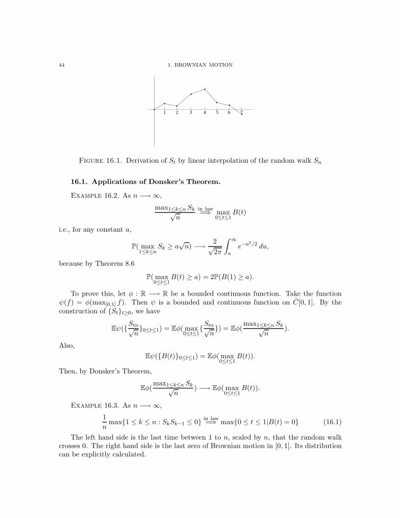
44 1. BROWNIAN MOTION
1 2 3 4 5 6 7
Figure 16.1. Derivation of St by linear interpolation of the random walk Sn
16.1. Applications of Donsker’s Theorem.
Example 16.2. As n −→ ∞,
max1≤k≤n Sk√n
in law=⇒ max0≤t≤1
B(t)
i.e., for any constant a,
P( max1≤k≤n
Sk ≥ a√n) −→ 2√
2π
∫ ∞
ae−u
2/2 du,
because by Theorem 8.6
P( max0≤t≤1
B(t) ≥ a) = 2P(B(1) ≥ a).
To prove this, let φ : R −→ R be a bounded continuous function. Take the functionψ(f) = φ(max[0,1] f). Then ψ is a bounded and continuous function on C[0, 1]. By theconstruction of Stt≥0, we have
Eψ(Stn√n0≤t≤1) = Eφ( max
0≤t≤1Stn√
n) = Eφ(
max1≤k≤n Sk√n
).
Also,Eψ(B(t)0≤t≤1) = Eφ( max
0≤t≤1B(t)).
Then, by Donsker’s Theorem,
Eφ(max1≤k≤n Sk√
n) −→ Eφ( max
0≤t≤1B(t)).
Example 16.3. As n −→ ∞,
1n
max1 ≤ k ≤ n : SkSk−1 ≤ 0 in law=⇒ max0 ≤ t ≤ 1|B(t) = 0 (16.1)
The left hand side is the last time between 1 to n, scaled by n, that the random walkcrosses 0. The right hand side is the last zero of Brownian motion in [0, 1]. Its distributioncan be explicitly calculated.
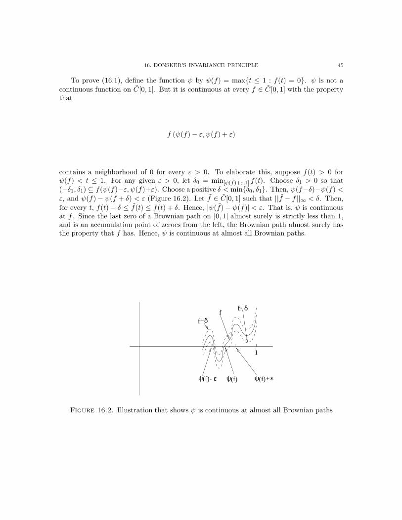
16. DONSKER’S INVARIANCE PRINCIPLE 45
To prove (16.1), define the function ψ by ψ(f) = maxt ≤ 1 : f(t) = 0. ψ is not acontinuous function on C[0, 1]. But it is continuous at every f ∈ C[0, 1] with the propertythat
f (ψ(f)− ε, ψ(f) + ε)
contains a neighborhood of 0 for every ε > 0. To elaborate this, suppose f(t) > 0 forψ(f) < t ≤ 1. For any given ε > 0, let δ0 = min[ψ(f)+ε,1] f(t). Choose δ1 > 0 so that(−δ1, δ1) ⊆ f(ψ(f)−ε, ψ(f)+ε). Choose a positive δ < minδ0, δ1. Then, ψ(f−δ)−ψ(f) <ε, and ψ(f)− ψ(f + δ) < ε (Figure 16.2). Let f ∈ C[0, 1] such that ||f − f ||∞ < δ. Then,for every t, f(t) − δ ≤ f(t) ≤ f(t) + δ. Hence, |ψ(f) − ψ(f)| < ε. That is, ψ is continuousat f . Since the last zero of a Brownian path on [0, 1] almost surely is strictly less than 1,and is an accumulation point of zeroes from the left, the Brownian path almost surely hasthe property that f has. Hence, ψ is continuous at almost all Brownian paths.
ψ(f)ψ(f) ψ(f)
1
+ε- ε
ff
f+
-
δ
δ
Figure 16.2. Illustration that shows ψ is continuous at almost all Brownian paths

46 1. BROWNIAN MOTION
Proof of Theorem 16.1. Let
Fn(t) =Stn√n, 0 ≤ t ≤ 1.
By Skorokhod embedding, there exist stopping times Tk, k = 1, 2, . . . for some standardBrownian motion B such that S(k) = B(Tk). Define Wn(t) = B(nt)√
n. Note that Wn is also
a standard Brownian motion. We will show that for any ε > 0, as n→ ∞,
P( sup0≤t≤1
|Fn −Wn| > ε) → 0. (16.2)
The theorem will follow since by (16.2) if ψ : C[0, 1] → R is bounded by M and iscontinuous on almost every Brownian motion path, then for any δ > 0,
P(∃f : ||W − f || < ε, |ψ(W )− ψ(f)| > δ) (16.3)
converges to 0 as ε→ 0. Now
|Eψ(Fn)− Eψ(Wn)| ≤ E|ψ(Fn) − ψ(Wn)|and the right hand side is bounded above by
2MP (||Wn − Fn|| ≥ ε) +2MP (||Wn − Fn|| < ε, |ψ(Wn) − ψ(Fn)| > δ) + δ.
The second term is bounded by (16.3), so by setting δ small, then setting ε small and thensetting n large, the three terms of the last expression may be made arbitrarily small.
To prove (16.2), let An be the event that |Fn(t) −Wn(t)| > ε for some t. We will showthat P(An) → 0.
Let k = k(t) designate the integer such that k−1n ≤ t < k
n . Then, since Fn(t) is linearlyinterpolated between Fn(k−1
n ) and Fn( kn),
An ⊂∃t :
∣∣∣S(k)√n
−Wn(t)∣∣∣ > ε
⋃∃t :
∣∣∣S(k − 1)√n
−Wn(t)∣∣∣ > ε
.
Writing S(k) = B(Tk) =√nWn(Tk/n), we get
An ⊂∃t :
∣∣∣Wn(Tkn
) −Wn(t)∣∣∣ > ε
⋃∃t :
∣∣∣Wn(Tk−1
n) −Wn(t)
∣∣∣ > ε.
Given δ ∈ (0, 1), the event on the right implies that either
∃t : |Tk/n− t| ∨ |Tk−1/n− t| ≥ δ (16.4)
or∃s, t ∈ [0, 2] : |s− t| < δ, |Wn(s) −Wn(t)| > ε.
Since each Wn is a standard Brownian motion, by choosing δ small, the probability of thelater event can be made arbitrarily small.
To conclude the proof, all we have to show is that for each δ, the probability of (16.4)converges to 0 as n → ∞. In fact, we will show that this event only happens for finitelymany n a.s. Since we chose k so that t is in the interval [(k − 1)/n, k/n], the absolute

17. HARMONIC FUNCTIONS AND BROWNIAN MOTION IN R d 47
differences in (16.4) are bounded above by the maximum of these distances when we lett = (k − 1)/n and k/n. This implies that (16.4) is a subset of the union of the events
sup0≤k≤n
|Tk − k + c|n
> δ (16.5)
for c = −1, 0 and c = 1. Note the deterministic fact that if a real sequence an satisfiesliman/n → 1, then sup0≤k≤n |ak − k|/n → 0. Since Tn is a sum of i.i.d. mean 1 randomvariables, the Law of Large Numbers enables us to apply this to an = Tn + c, and concludethat (16.5) happens only finitely many times, as desired.
17. Harmonic functions and Brownian motion in Rd
Definition 17.1. Let D ⊂ Rd be a domain (a connected open set). u : D → R is
harmonic if it is measurable, locally bounded (i.e. bounded on closed balls in D) and forany ball B = B(x, r) ⊂ D,
u(x) =1
Ld(B)
∫Bu(y)dy.
Remark. If u is harmonic in D, then it is continuous in D: If xn → x then
u(y)1(B(xn, r))(y)a.e.−→n→∞u(y)1(B(x, r))(y),
thus, by the Dominated Convergence Theorem, u(xn) → u(x).
Theorem 17.2. Let u be measurable and locally bounded in D. Then, u is harmonic inD iff:
u(x) =1
σd−1(S(x, r))
∫S(x,r)
u(y)dσd−1(y), (17.1)
where S(x, r) = y : |y − x| = r, and σd−1 is the (d− 1)-dimensional Hausdorff measure.
Proof. Assume u is harmonic. Define:∫S(x,r)
u(y)dσd−1(y) = Ψ(r)rd−1.
We will show that Ψ is constant. Indeed, for any R > 0,
RdLd(B(x, 1))u(x) = Ld(B(x, R))u(x) =∫B(x,R)
u(y)dy =∫ R
0Ψ(r)rd−1dr.
Differentiate w.r.t. R to obtain:
dLd(B(x, 1))u(x) = Ψ(R).
and therefore Ψ(R) is constant. It follows from the well known identity dLd(B(x, r))/r =σd−1(S(x, r)) that (17.1) holds.
For the other direction, note that (17.1) implies that u(x) = Ld(B(x, r))−1∫B(x,r) u(y)dy
by Fubini’s Theorem.
Remark. Here is an equivalent definition for harmonicity. u is harmonic if u is contin-uous, twice differentiable, and ∆u =
∑i∂2u
(∂xi)2= 0.

48 1. BROWNIAN MOTION
Definition 17.3.
G(x, y) =∫ ∞
0p(x, y, t)dt, x, y ∈ R
d
is the Green function in Rd, where p(x, y, t) is the Brownian transition density function,
p(x, y, t) = (2πt)−d/2 exp(− |x−y|2
2t
).
Proposition 17.4. The Green function G satisfies:
(1) G(x, y) is finite iff x 6= y and d > 2.(2) G(x, y) = G(y, x) = G(y − x, 0).(3) G(x, 0) = cd|x|2−d where cd = Γ(d/2 − 1)/(2πd/2).
Proof. Facts 1. and 2. are immediate. For 3., note that:
G(x, 0) =∫ ∞
0
(2πt)−d/2 exp(− |x|2
2t
)dt.
Substituting s = |x|22t , we obtain:
G(x, 0) =∫ ∞
0
(π|x|2s
)−d/2e−s|x|22s2
ds = |x|2−dπ−d/2
2
∫ ∞
0
e−ssd2−2ds.
(The integral is known as Γ(d2 − 1)).
One probabilistic meaning of G is given in the following proposition:
Proposition 17.5. Define Fr(x) =∫B(0,r)G(x, z)dz. Then:
Fr(x) = Ex
∫ ∞
01(Wt ∈ B(0, r))dt. (17.2)
In words: Fr(x) is the expected time the Brownian motion started at x spends in B(0, r).
Proof. By Fubini’s Theorem and the definition of the Markov kernel p,, we have
Fr(x) =∫ ∞
0
∫B(0,r)
p(x, z, t)dzdt =∫ ∞
0Px(W (t) ∈ B(0, r))dt
Applying Fubini another time,
Fr(x) = Ex
∫ ∞
01(Wt ∈ B(0, r))dt, (17.3)
as needed.
Theorem 17.6. For d ≥ 3: x 7→ G(x, 0) is harmonic on Rd \ 0.
Proof. We prove that Fε(x) is harmonic in Rd \B(0, ε), i.e.
Fε(x) =1
Ld(B(x, r))
∫B(x,r)
Fε(y)dy. (17.4)

17. HARMONIC FUNCTIONS AND BROWNIAN MOTION IN R d 49
for 0 < r < |x| − ε. The theorem will follow from (17.4) since as G is continuous we have:
G(x, 0) = limε→0
Fε(x)Ld(B(0, ε))
= limε→0
1Ld(B(0, r))
∫B(x,r)
Fε(y)Ld(B(0, ε))
dy
=1
Ld(B(x, r))
∫B(x,r)
G(y, 0)dy,
where the last equality follows from the bounded convergence theorem.Denote by νd−1 = σd−1/||σd−1|| the rotation-invariant probability measure on the unit
sphere in Rd. Fix x 6= 0 in R
d, let 0 < r < |x| and let ε < |x| − r. Denote τ = mint :|W (t) − x| = r. Since W spends no time in B(0, ε) before time τ , we can write Fε(x) as
Ex
∫ ∞
τ1(Wt ∈ B(0, ε))dt = ExEx
[∫ ∞
τ1(Wt ∈ B(0, ε))dt|Wτ
]By the strong Markov property and since Wτ is uniform on the sphere of radius r about xby rotational symmetry, we conclude:
Fε(x) = ExFε(Wτ ) =∫S(0,1)
Fε(x+ ry)dνd−1(y).
Hence (17.4) follows from Theorem 17.2. This proves Theorem 17.6
We have therefore proved that x 7→ 1|x|d−2 is harmonic in R
d \ 0, d ≥ 3.For d ≥ 3, the time Brownian motion spends in any ball around the origin has ex-
pectation FR(0) by (17.2). By the definition of FR(0), this expectation can be writtenas ∫
B(0,R)G(0, x)dx= cd
∫B(0,R)
|x|2−ddx = cd
∫ R
0rd−1r2−ddr = c′dR
2,
in particular, it is finite.We now wish to show that Brownian motion in R
d, d ≥ 3 is transient.
Proposition 17.7. For d ≥ 3 and |x| > r,
hr(x)def= Px
(∃t ≥ 0 : Wt ∈ B(0, r)
)=( r
|x|)d−2
.
Proof. Recall the definition of Fr(x)
Fr(x) =∫B(0,r)
G(x, z)dz =∫B(0,r)
G(x− z, 0)dz. (17.5)
Since G is harmonic, from (17.5) we have
Fr(x) = Ld(B(0, r))G(x, 0) = Ld(B(0, r))cd|x|2−d.In particular, Fr(x) depends only on |x|. We define Fr(|x|) = Fr(x).
Suppose |x| > r. Since Fr(x) is the expected time spent in B(0, r) starting from x, itmust equal the probability of hitting S(0, r) starting from x, times the expected time spent

50 1. BROWNIAN MOTION
in B(0, r) starting from the hitting point of this sphere. Therefore Fr(x) = hr(x)Fr(r).
This implies hr(x) =(r|x|)d−2
.
Proposition 17.8. Brownian motion in dimension d ≥ 3 is transient, i.e., limt→∞ |W (t)|= ∞.
Proof. We use the fact that lim supt→∞ |W (t)| = ∞ a.s. Therefore, for any 0 < r < R,
P(BM visits B(0, r) for arbitrarily large t)≤ P(BM visits B(0, r) after hitting S(0, R))
=( rR
)d−2,
which goes to 0 as R → ∞. The proposition follows.
We are now also able to calculate the probability that a Brownian motion startingbetween two spheres will hit the smaller one before hitting the larger one.
Proposition 17.9. Define
a = Px(Brownian motion hits S(0, r) before S(0, R)),
where r < |x| < R. Then
a =
(r|x|)d−2 − ( rR)d−2
1 − ( rR)d−2. (17.6)
Proof. It follows from Proposition 17.7 and the strong Markov property that
a = Px(BM hits S(0, r))− Px(BM hits S(0, R) first and then hits S(0, r))
=(r
|x|)d−2
− (1− a)( rR
)d−2. (17.7)
Solving (17.7), we get (17.6).
Remark. Since a is fixed under scaling, the visits of Brownian motion to S(0, ek), k ∈ Z
form a discrete random walk with constant probability to move up (k increasing) or down(k decreasing). The probability to move down is
e2−d − e4−2d
1 − e4−2d.
It is easy to see that this probability is less than 1/2 (This also follows from the fact thatthe Brownian motion is transient, and therefore the random walk should have an upwarddrift).
18. Maximum principle for harmonic functions
Proposition 18.1 (Maximum Principle). Suppose that u is harmonic in D ⊂ Rd where
D is a connected open set.(i) If u attains its maximum in D, then u is a constant.(ii) If u is continuous on D and D is bounded, then maxD u = max∂D u.

19. THE DIRICHLET PROBLEM 51
(iii) Assume that D is bounded, u1 and u2 are two harmonic functions on D which arecontinuous on D. If u1 and u2 take the same values on ∂D, then they are identical on D.
Proof.
(i) Set M = supD u. Note that V = x ∈ D : u(x) = M is relatively closed in D. SinceD is open, for any x ∈ V , there is a ball B(x, r) ⊂ D. By the mean-value property of u,
u(x) =1
Ld(B(x, r))
∫B(x,r)
u(y)dy ≤M
Equality holds iff u(y) = M almost everywhere on B(x, r), or, by continuity, B(x, r) ⊂ VThis means that V is also open. Since D is connected we get that V = D. Therefore, u isconstant on D.
(ii) supD u is attained on D since u is continuous and D is closed and bounded. Theconclusion now follows from (i).
(iii) Consider u1 − u2. It follows from (ii) that
supD
(u1 − u2) = sup∂D
(u1 − u2) = 0.
Similarly infD(u2 − u1) = 0. So u1 = u2 on D.
Corollary 18.2. Suppose that u is a radial harmonic function in D ≡ r < |x| <R ⊂ R
d (“radial” means u(x) = u(|x|) for some function u and all x) and u is continuouson D.
If d ≥ 3, there exist constants a and b such that u(x) = a+ b|x|2−d.If d = 2, there exist constants a and b such that u(x) = a+ b log |x|.Proof. For d ≥ 3, choose a and b such that
a+ br2−d = u(r),
anda+ bR2−d = u(R).
Notice that harmonic function u(x) = u(|x|) and the harmonic function x → a + b|x|2−dagree on ∂D. They also agree on D by Proposition 18.1. So u(x) = a+ b|x|2−d. By similarconsideration we can show that u(x) = a + b log |x| in the case d = 2.
19. The Dirichlet problem
Definition 19.1. Let D ⊂ Rd be a domain. We say that D satisfies the Poincare
Cone Condition if for each point x ∈ ∂D there exists a cone Cx(α, h) of height h(x) andangle α(x) s.t. Cx(α, h) ⊂ Dc and Cx(α, h) is based at x.
Proposition 19.2 (Dirichlet Problem). Suppose D ⊂ Rd is a bounded domain with
boundary ∂D, s.t. D satisfies the Poincare Cone condition, and f is a continuous functionon ∂D. Then there exists a unique function u which is harmonic on D and is an “extension”of f in the sense that
limx→a,x∈D
u(x) = f(a) (19.1)
for each a ∈ ∂D.

52 1. BROWNIAN MOTION
Proof. The uniqueness claim follows from Proposition 18.1. To prove existence, let Wbe a Brownian motion in R
d and define
u(x) = Exf(Wτ∂D), where τA = inft ≥ 0 : Wt ∈ A
for any Borel set A ⊂ Rd. For a ball B(x, r) ⊂ D, the strong Markov property implies that
u(x) = Ex[Ex[f(Wτ∂D)|FτS(x,r)
]] = Ex[u(WτS(x,r))] =
∫S(x,r)
u(y)µr(dy),
where µr is the uniform distribution on the sphere S(x, r). Therefore, u has the mean valueproperty and so it is harmonic on D (by Theorem 17.2).
It remains to be shown that the Poincare Cone Condition implies (19.1). Fix z ∈ ∂D,then there is a cone with height h > 0 and angle α > 0 in Dc based at z. Let
φ = supx∈B(0, 1
2)
Px[τS(0,1) < τC0(α,1)].
Then φ < 1. Note that if x ∈ B(0, 2−k) then by the strong Markov property:
Px[τS(0,1) < τC0(α,1)] ≤k−1∏i=0
supx∈B(0, 1
2−k+i )
Px[τS(0,2−k+i+1) < τC0(α,2−k+i+1)] = φk.
Therefore, for any positive integer k and h′ > 0, we have
Px[τS(z,h′) < τCz(α,h′)] ≤ φk
for all x with |x− z| < 2−kh′.Given ε > 0, there is a 0 < δ ≤ h such that |f(y) − f(z)| < ε for all y ∈ ∂D with
|y − z| < δ. For all x ∈ D with |z − x| < 2−kδ,
|u(x) − u(z)| = |Exf(Wτ∂D) − f(z)| ≤ Ex|f(Wτ∂D
) − f(z)| (19.2)
If the Brownian motion hits the cone Cz(α, δ), which is outside the domain D, before thesphere S(z, δ), then |z −Wτ∂D| < δ, and f(Wτ∂D
) is close to f(z). The complement hassmall probability. More precisely, (19.2) is bounded above by
2‖f‖∞PxτS(z,δ) < τCz(α,δ) + εPxτD < τS(z,δ) ≤ 2‖f‖∞φk + ε.
Hence u is continuous on D.
20. Polar points and recurrence
Given x ∈ R2, 1 ≤ |x| ≤ R, we know that
Px[τS(0,R) < τS(0,1)] = a+ b log |x|.Since the left-hand side is clearly a function of |x|, and it is a harmonic function of x for1 < |x| < R by averaging over a small sphere surrounding x. Setting |x| = 1 impliesa =0, and |x| = R implies b = 1
logR . It follows that
Px[τS(0,R) < τS(0,1)] =log |x|logR
.

20. POLAR POINTS AND RECURRENCE 53
By scaling, for 0 < r < R and r ≤ |x| ≤ R,
Px[τS(0,R) < τS(0,r)] =log |x|
r
log Rr
. (20.1)
Definition 20.1. A set A is polar for a Markov process X if for all x
Px[Xt ∈ A for some t > 0] = 0
The image of Brownian motion is the random set
BM(δ,∞) def= ∪δ<t<∞Wt.Proposition 20.2. Points are polar for a planar Brownian motion, that is for all z ∈ R
2
we have P0z ∈ BM(0,∞) = 0.
Proof. Take z 6= 0 and 0 < ε < |z| < R,
P0τS(z,R) < τS(z,ε) =log |z|
ε
log Rε
.
Let ε → 0+,P0τS(z,R) < τz = lim
ε→0+P0τS(z,R) < τS(z,ε) = 1.
and thenP0τS(z,R) < τz for all integersR > |z| = 1
It follows thatP0z ∈ BM(0,∞) = P0τz <∞ = 0.
Given δ > 0, by Markov property and state homogeneity of Brownian motion,
P00 ∈ BM(δ,∞) = E0[PXδ0 ∈ BM(0,∞)] = 0.
Let δ → 0+, we haveP00 ∈ BM(0,∞) = 0.
Hence any fixed single point is a polar set for a planar Brownian motion.
The expected area E0[L2(BM(0,∞))] of planar Brownian motion can be written as
E0[∫
R 2Iz∈BM (0,∞)dz] =
∫R 2
P0z ∈ BM(0,∞)dz = 0,
where the first equality is by Fubini, the second from the previous theorem. So almostsurely, the image of a planar Brownian motion is a set with zero Lebesgue measure.
Proposition 20.3. Planar Brownian motion is neighborhood recurrent. i.e.
P0BM(0,∞)is dense in R2 = 1.
Proof. Note that lim supt→∞ |Wt| = ∞, so for all z ∈ R2 and ε > 0,
P0τB(z,ε) = ∞ = limR→∞
P0τS(z,R) < τB(z,ε) = 0.
Summing over all rational z and ε completes the proof.

54 1. BROWNIAN MOTION
Question: Let W be a Brownian motion in R3. Is there an infinite cylinder avoided by
W? Or equivalently, what is the value of
P0All orthogonal projections of W are neighborhood recurrent?In fact, an avoided cylinder does exist a.s., so the probability in the last display vanishes.This is due to Adelman, Burdzy and Pemantle (1998): Sets avoided by Brownian motion.Ann. Probab. 26, 429–464.
21. Capacity and harmonic functions
In this section we will characterize the sets that BM hits, and give bounds on the hittingprobabilities in terms of capacity.
The central question of this section is the following: which sets Λ ⊂ Rd does Brownian
motion hit with positive probability? This is related to the following question: for whichΛ ⊂ R
d are there bounded harmonic functions on Rd \ Λ?
Consider the simplest case first. When Λ is the empty set, the answer to the firstquestion is trivial, whereas the answer to the second one is provided by Liouville’s theorem.We will give a probabilistic proof of this theorem.
Theorem 21.1. For d ≥ 1 any bounded harmonic function on Rd is constant.
Proof. Let u : Rd → [−M,M ] be a harmonic function, x, y two distinct points in R
d,and H the hyperplane so that the reflection in H takes x to y.
Let Wt be Brownian motion started at x, and W t its reflection in H . Let τH = mint :W (t) ∈ H. Note that
Wtt≥τH d= W tt≥τH . (21.1)Harmonicity implies that
Eu(Wt) = E(E(u(Wt)| |W (t) − x|)) = E(u(x)) = u(x)
since the conditional expectation above is just the average u on a sphere about x of radius|W (t) − x|. Decomposing the above into t < τH and t ≥ τH we get
u(x) = Exu(Wt1(t < τH)) + Exu(Wt1(t ≥ τH)).
A similar equality holds for u(y). Now using (21.1):
|u(x)− u(y)| = |Eu(Wt1(t < τH))− Eu(W t1(t < τH))| ≤ 2MP(t < τH) → 0
as t → ∞. Thus u(x) = u(y), and since x and y were chosen arbitrarily, u must beconstant.
A stronger result is also true.
Theorem 21.2. For d ≥ 1, any positive harmonic function on Rd is constant.
Proof. Let x, y ∈ Rd, a = |x − y|. Suppose u is a positive harmonic function. Then
u(x) can be written as
1LdBR(x)
∫BR(x)
u(z)dz ≤ LdBR+a(y)LdBR(x)
1LdBR+a(y)
∫BR+a(y)
u(z)dz =(R+ a)d
Rdu(y)

21. CAPACITY AND HARMONIC FUNCTIONS 55
This converges to u(y) as R → ∞, so u(x) ≤ u(y), and by symmetry, u(x) = u(y) forall x, y. Hence u is constant.
Nevanlinna (about 1920) proved that for d ≥ 3 there exist non-constant boundedharmonic functions on R
d \ Λ iff CapG(Λ) > 0. Here G denotes the Green functionG(x, y) = c|x − y|2−d. It was proved later that dimΛ > d − 2 implies existence of suchfunctions, and dim Λ < d−2 implies nonexistence. Kakutani (1944) showed that there existsuch functions iff P(BM hits Λ) > 0. Note that the Green function is translation invari-ant, while the hitting probability of a set is invariant under scaling. It is therefore betterto estimate hitting probabilities by a capacity function with respect to a scale-invariantmodification of the Green kernel, called the Martin kernel:
K(x, y) =G(x, y)G(0, y)
=|y|d−2
|x− y|d−2
for x 6= y in Rd, and K(x, x) = ∞. The following theorem shows that Martin capacity is
indeed a good estimate of the hitting probability.
Theorem 21.3 (Benjamini, Pemantle, Peres 1995). Let Λ be any closed set in Rd, d ≥ 3.
Then12
CapK Λ ≤ P(∃t > 0 : W (t) ∈ Λ) ≤ CapK(Λ) (21.2)
Here
CapK(Λ) =[
infµ(Λ)=1
∫Λ
∫ΛK(x, y)dµ(x)dµ(y)
]−1
.
Proof. To bound the probability of ever hitting Λ from above, consider the stoppingtime τ = mint : Wt ∈ Λ. The distribution of Wτ on the event τ < ∞ is a possiblydefective distribution ν satisfying
ν(Λ) = P(τ <∞) = P(∃t > 0 : W (t) ∈ Λ). (21.3)
Now recall the standard formula, valid when 0 < ε < |y|:
P(∃t > 0 : |Wt − y| < ε) =( ε
|y|)d−2
. (21.4)
By a first entrance decomposition, the probability in (21.4) is at least
P(|Wτ − y| > ε and ∃t > τ : |Wt − y| < ε) =∫x:|x−y|>ε
εd−2dν(x)|x− y|d−2
.
Dividing by εd−2 and letting ε→ 0 we obtain∫Λ
dν(x)|x− y|d−2
≤ 1|y|d−2
,
i.e.∫ΛK(x, y)dν(x) ≤ 1 for all y ∈ Λ. Therefore, if
Ik(ν) =∫
Λ
∫Λ
|y|d−2dν(x)dν(y)|x− y|d−2
,

56 1. BROWNIAN MOTION
then IK(ν) ≤ ν(Λ) and thus if we use νν(Λ) as a probability measure we get:
CapK(Λ) ≥ [IK(ν/ν(Λ))]−1 ≥ ν(Λ),
which by (21.3) yields the upper bound on the probability of hitting Λ.To obtain a lower bound for this probability, a second moment estimate is used. It is
easily seen that the Martin capacity of Λ is the supremum of the capacities of its compactsubsets, so we may assume that Λ is itself compact. For ε > 0 and y ∈ R
d let Bε(y)denote the Euclidean ball of radius ε about y and let hε(|y|) denote the probability that thestandard Brownian path hits this ball, that is (ε/|y|)d−2 if |y| > ε, and 1 otherwise.
Given a probability measure µ on Λ, and ε > 0, consider the random variable
Zε =∫
Λ
1(∃t > 0 : Wt ∈ Bε(y))hε(|y|)−1dµ(y).
Clearly EZε = 1. By symmetry, the second moment of Zε can be written as:
EZ2ε = 2E
∫Λ
∫Λ
1(∃t > 0 : Wt ∈ Bε(x), ∃s > t : Ws ∈ Bε(y))dµ(x)dµ(y)hε(|x|)hε(|y|)
≤ 2E
∫Λ
∫Λ
1(∃t > 0 : Wt ∈ Bε(x))hε(|y − x| − ε)hε(|x|)hε(|y|) dµ(x)dµ(y)
= 2∫
Λ
∫Λ
hε(|y − x| − ε)hε(|y|) dµ(x)dµ(y) (21.5)
The last integrand is bounded by 1 if |y| ≤ ε. On the other hand, if |y| > ε and|y − x| ≤ 2ε then hε(|y − x| − ε) = 1 ≤ 2d−2hε(|y − x|), so that the integrand on the righthand side of (21.5) is at most 2d−2K(x, y). Thus
EZ2ε ≤ 2µ(Bε(0)) + 2d−1
∫ ∫1(|y − x| ≤ 2ε)K(x, y)dµ(x)dµ(y)
+2∫ ∫
1(|y − x| > 2ε)( |y||y − x| − ε
)d−2
dµ(x)dµ(y). (21.6)
Since the kernel is infinite on the diagonal, any measure with finite energy must haveno atoms. Restricting attention to such measures µ, we see that the first two summands in(21.6) drop out as ε → 0 by dominated convergence. Thus by the dominated convergenceTheorem,
limε↓0
EZ2ε ≤ 2IK(µ). (21.7)
Clearly the hitting probability P(∃t > 0, y ∈ Λ : Wt ∈ Bε(y)) is at least
P(Zε > 0) ≥ (EZε)2
EZ2ε
= (EZ2ε )
−1.
Transience of Brownian motion implies that if the Brownian path visits every ε-neighborhoodof the compact set Λ then it almost surely intersects Λ itself. Therefore, by (21.6):
P(∃t > 0, : Wt ∈ Λ) ≥ limε↓0
(EZ2ε )
−1 ≥ 12IK(µ)
.

22. KAUFMAN’S THEOREM ON UNIFORM DIMENSION DOUBLING 57
Since this is true for all probability measures µ on Λ, we get the desired conclusion:
P(∃t > 0 : Wt ∈ Λ) ≥ 12
CapK(Λ).
Remark. The right-hand inequality in (21.2) can be an equality– a sphere centered atthe origin has hitting probability and capacity both equal to 1. The next exercise showsthat the constant 1/2 on the left cannot be increased.
Exercise 21.4. Consider the spherical shell
ΛR = x ∈ Rd : 1 ≤ |x| ≤ R.
Show that limR→∞ CapK(ΛR) = 2.
22. Kaufman’s theorem on uniform dimension doubling
In the previous sections we have seen the dimension doubling property of Brownianmotion: for any set A, we have dimW (A) = 2 dim(A) a.s. For d ≥ 2 this is true for allclosed sets a.s. To see the distinction, consider the zero set of 1 dimensional Brownianmotion.
Lemma 22.1. Consider a cube Q ⊂ Rd centered at a point x and having diameter 2r.
Let W be Brownian motion in Rd, with d ≥ 3. Define recursively
τ1 = inft ≥ 0 : W (t) ∈ Qτk+1 = inft ≥ τk + r2 : W (t) ∈ Q
with the usual convention that inf ∅ = ∞. There exists a positive θ = θd < 1 which does notdepend on r and z, such that Pz(τn+1 <∞) ≤ θn.
Proof. It is sufficient to show that for some θ as above,
Pz(τk+1 = ∞ | τk <∞) > 1 − θ.
But the quantity on the right can be bounded below by
Pz(τk+1 = ∞| |W (τk + r2) − x| > 2r, τk <∞)Pz(|W (τk + r2) − x| > 2r|τk <∞)
The second factor is clearly positive, and the first is also positive since W is transient. Bothprobabilities are invariant under changing the scaling factor r.
Corollary 22.2. Let Dm denote the set of binary cubes of side length 2−m inside[−1
2 ,12 ]d. A.s. there exists a random variable C(ω) so that for all m and for all cubes
Q ∈ Dm we have τQK+1 = ∞ with K = C(ω)m.
Proof. ∑m
∑Q∈Dm
P(τQdcm+1e <∞) ≤∑m
2dmθcm
Choose c so that 2dθc < 1. Then by Borel-Cantelli, for all but finitely many m we haveτQdcm+1e+1
= ∞ for all Q ∈ Dm. Finally, we can choose a random C(ω) > c to handle theexceptional cubes.

58 1. BROWNIAN MOTION
Theorem 22.3 (Kaufman’s Uniform Dimension Doubling for d ≥ 3).
P(dimW (A) = 2 dimA for all closed A ⊂ [0,∞]) = 1 (22.1)
Proof. The ≤ direction holds in all dimensions by the Holder property of Brownianmotion (see Corollary 4.3 and Lemma 5.11).
Fix L. We will show that with probability one, for all closed subsets S of [−L, L]d wehave
dimW−1(S) ≤ 12
dimS. (22.2)
Applying this to S = W (A)∩[−L, L]d for a countable unbounded set of L we get the desiredconclusion. By scaling, it is sufficient to prove (22.2) for L = 1
2 . We will verify this forthe paths satisfying Corollary 22.2; these have full measure. The rest of the argument isdeterministic, we fix an ω to be such a path.
For β > dimS and for all ε there exist covers of S by binary cubes Qj in⋃mDm so
that∑ |Qj|β < ε. If Nm denotes the number of cubes from Dm in such a cover, then∑
m
Nm2−mβ < ε.
Consider the W -inverse image of these cubes. Since we chose ω so that Corollary 22.2is satisfied, this yields a cover of W−1(S), which for each m ≥ 1 uses at most C(ω)mNm
intervals of length r2 = d2−2m.For β1 > β we can bound the β1/2 dimensional Hausdorff content of W−1 above by
∞∑m=1
C(ω)mNm(d2−2m)β1/2 = C(ω)dβ1/2∞∑m=1
mNm2−mβ1 .
This can be made small by choosing a suitable ε. Thus W−1(S) has Hausdorff dimensionat most β/2 for all β > dimS, and therefore dimW−1(S) ≤ dimS/2.
In two dimensions we cannot rely on transience of Brownian motion. To get around thisproblem, we can look at the Brownian path up to a stopping time. A convenient one is
τ∗R = mint : |W (t)| = R.For the two dimensional version of Kaufman’s theorem it is sufficient to show that
P(dimW (A) = 2 dim(A ∩ [0, τ∗R]) for all closed A ⊂ [0,∞]) = 1.
Lemma 22.1 has to be changed accordingly. Define τk as in (22.1), and assume that thecube Q is inside the ball of radius R about 0. Then we have
Lemma 22.4.Pz(τk < τ∗R) ≤
(1 − c
m
)k ≤ e−ck/m (22.3)
Here c = c(R) > 0, 2−m−1 < r < 2−m, and z is any point in Rd.
Proof. It suffices to bound Pz(τk+1 ≥ τ∗R | τk < τ∗R) from below by
Pz(τk+1 ≥ τ∗R| W (τk + r2) > 2r, τk < τ∗R)Pz(|W (τk + r2) − x| > 2r |τk < τ∗R)
The second factor does not depend on r and R, and it can be bounded below by a constant.The first factor is bounded below be the probability that planar Brownian motion started

23. PACKING DIMENSION 59
at distance 2r from the origin hits the sphere of radius 2R before the sphere of radius r(both centered at the origin). Using (20.1), this is given by
log22rr
log22Rr
≥ 1log2(R+ 1 +m)
.
This is at least c1/m for some c1 which depends on R only.
The bound (22.3) on P (τk <∞) in two dimensions is worse by a linear factor than thebound in higher dimensions. This, however, does not make a significant difference in theproof of the two dimensional version of Theorem 22.3.
Exercise 22.5. Prove Theorem 22.3 for two dimensional Brownian motion.
23. Packing dimension
Tricot (1980, 1982) introduced packing dimension, which plays a dual role to Haus-dorff dimension in many settings. For our present purpose, the representation of packing di-mension which is convenient to use as a definition, is as a regularization of upper Minkowskidimension:
dimp(A) = infA⊂∪jAj
supj
dimM(Aj) ,
where the infimum is over all countable covers of A. (See Tricot (1982), Proposition 2,or Falconer (1990), Proposition 3.8.) The infimum may also be taken only over countablecovers of A with closed sets since dimM(Aj) = dimM(Aj).
Note that for packing dimension, unlike the Minkowski dimension, the following prop-erty holds for any partition Aj , j = 1, 2, . . . of A:
dimpA = supj
dimpAj.
Part (i) of the next lemma is due to Tricot (1982) (see also Falconer 1990); Part (ii) fortrees can be found in Benjamini and Peres (1994, Proposition 4.2(b)); the general versiongiven is in Falconer and Howroyd (1994) and in Mattila and Mauldin (1994).
Lemma 23.1. Let A be a closed subset of R.(i) If any open set V which intersects A satisfies dimM(A∩V ) ≥ α , then dimp(A) ≥ α.(ii) If dimp(A) > α, then there is a (relatively closed) nonempty subset A of A, such
that dimp(A ∩ V ) > α for any open set V which intersects A.
Proof. (i) Let A ⊂ ∪∞j=1Aj, where the Aj are closed. We are going to show that
there exist an open set V and an index j such that V ⊂ Aj. For this V and j we have:dimM(Aj) ≥ dimM(Aj ∩ V ) = dimM(A ∩ V ) ≥ α. This in turn implies that dimp(A) ≥ α.If Aj is closed and for any V open s.t. V ∩ A 6= ∅, it holds that V 6⊂ Aj , then Acj is adense open set relative to A. By Baire’s category theorem A ∩⋂j Acj 6= ∅, i.e., A 6⊂ ⋃j Aj.Therefore, if A ⊂ ⋃j Aj then there exists an open set, V , s.t. V ∩ A 6= ∅ and s.t. V ⊂ Aj.
(ii) Define
A = A \⋃
J rational interval : dimM(J ∩ A) ≤ α.

60 1. BROWNIAN MOTION
Then, any countable cover of A together with the sets removed on the right yields a count-able cover of A, giving dimp A ∨ α ≥ dimpA > α. Since A ⊂ A, we conclude thatdimp A = dimpA > α. If for some V open, V ∩ A 6= ∅ and dimp(A ∩ V ) ≤ α then V
contains some rational interval J s.t. A ∩ J 6= ∅. For that J,
dimp(A ∩ J) ≤ max(dimp(A \ A), dimp(A ∩ J))
≤ max(α, dimp(A ∩ V )) = α,
contradicting the construction of A.
24. Hausdorff dimension and random sets
Fix p. For n ≥ 0, define Qn(p), to be random subsets of [0, 1] as follows. For n > 1,0 ≤ i < 2i let Uni be i.i.d. random variables uniform on [0, 1]. Let
Qn(p) =⋃
i : Uni ≤p
(i2−n, (i+ 1)2−n
)Define Q(p) =
⋂nQ
n(p).We call an interval I a binary interval if it is of the form end (i2−n, (i+ 1)2−n) for
some integers i, n. Note that each interval I can be covered by two closed binary intervalsof length at most |I |. Thus we can require covers to be made of binary intervals in thedefinition Hausdorff dimension for subsets of R.
Lemma 24.1. If A ⊂ [0, 1] intersects the random set Q(2−α) with positive probabilitythen dimH(A) ≥ α.
Proof. Let b = P(A∩Q(2−α)). Then for any countable collection of binary subintervalsof [0, 1] s.t. A ⊂ ⋃j Ij we have
b ≤∑j
P(Ij ∩Q(2−α) 6= ∅) ≤∑j
P(Ij ∩Qnj (2−α) 6= ∅)
Here nj is defined so that Ij is of length 2−nj . Thus the summand on the right equals(2−α)nj = |Ij|α. Therefore b ≤∑j |Ij|α. However, if dimH(A) = α1 < α, then there existsa collection of binary intervals Ij s.t. A ⊂ ⋃j Ij and s.t.
∑j |Ij|α < b.
Corollary 24.2. If a random set A ⊂ [0, 1] intersects the independent random setQ(2−α) with positive probability then ||dimH(A)||∞ ≥ α.
Proof. By assumption
0 < P(A∩Q 6= ∅) = EP(A ∩Q 6= ∅|A).
By the previous lemma, when P(A ∩Q 6= ∅|A) > 0 we also have dimHA ≥ α, so the righthand side equals
E [1(dimHA ≥ α)P(A ∩Q 6= ∅|A)] ≤ E1(dimHA ≥ α)= P(dimHA ≥ α).
Lemma 24.3. If a random set A has P(A∩K 6= ∅) > 0 for all fixed K s.t. dimHK ≥ β,then ||dimH(A)||∞ ≥ 1 − β.

25. AN EXTENSION OF LEVY’S MODULUS OF CONTINUITY 61
Proof. We show that ||dimHQ(2−α)||∞ ≥ 1 − α. The hypothesis of the lemma willthen imply that for Q independent of A, P(A∩Q(2−(1−β−ε)) 6= ∅) > 0 and thus by Corollary24.2 ||dimH(A)||∞ ≥ 1 − β.
Let Q1, Q2 be two independent random sets s.t. Q1d= Q(2−α) and Q2
d= Q(2α−1+ε).Then Q1∩Q2
d= Q(2ε−1). By the theory of branching processes, P(Q(2ε−1) 6= ∅) > 0. Thus,using Corollary 24.2 again, and taking ε→ 0,∣∣∣∣dimHQ(2−α)
∣∣∣∣∞ ≥ 1− α.
25. An extension of Levy’s modulus of continuity
The following technical lemma is closely related to the discussion in the previous section.After stating it, we show how it implies a lower bound on the modulus of continuity forBrownian motion.
Lemma 25.1. Suppose that for each n and open binary interval I ⊂ [0, 1] of length 2−nwe have an indicator random variable ZI with P(ZI = 1) = pn. Suppose further that if|I | = |J| and dist(I, J) > cn
2n , then ZI and ZJ are independent. Let
An =⋃I : |I | = 2−n, ZI = 1,
A = lim supn→∞
An =⋂n
⋃m≥nAn.
If we have
lim infn→∞
log2 pnn
≥ −θ,then for any fixed E ⊂ [0, 1] closed, the following statements hold:
(i) If dimpE > θ, then P(E ∩A 6= ∅) = 1,(ii) ||dimHA||∞ ≥ 1− θ.
We will now use this lemma to prove the lower bound for the modulus of continuity ofBrownian motion in a prescribed set.
Theorem 25.2. Let ϕ(h) = (2h log(1/h))1/2, and let E ⊂ [0, 1] be a closed set. Then
supt∈E
lim suph↓0
|Bt+h −Bt|ϕ(h)
≥√dimpE. (25.1)
Moreover, the set of times
Fλ =t ∈ [0, 1]
∣∣∣ lim suph↓0
|Bt+h − Bt|ϕ(h)
≥ λ
(25.2)
satisfies ‖ dimH(Fλ)‖∞ ≥ 1 − λ2.
In fact, the inequality in (25.1) is an equality, see D. Khoshnevisan, Y. Peres andY. Xiao, Limsup random fractals, Elect. J. Probab., 5 (2000), paper 4, 1–24. The caseE = [0, 1] is Levy’s modulus of continuity theorem. The set Fλ defined in (25.2) is theset of “λ-fast points” for Brownian motion; Orey and Taylor (1974) showed that it hasHausdorff dimension 1 − λ2 almost surely.

62 1. BROWNIAN MOTION
Proof. For each binary interval I = (a2−n, (a + 1)2−n), set the indicator variableZI = 1 iff the following two conditions hold:
supt∈I
∣∣B(t) −B((a + 1)2−n)∣∣ ≤ 2−n/2, (25.3)∣∣B((a+ n)2−n) −B((a + 1)2−n)∣∣ ≥ λϕ((n− 1)2−n). (25.4)
Suppose that ZI = 1. For t ∈ I , set h = (a + n)2−n − t, so that h ∈ ((n−1)2−n, n2−n).Using the triangle inequality we get
|B(t+ h) − B(t)| ≥ λϕ((n− 1)2−n) − 2−n/2. (25.5)
Dividing the left and right hand side of (25.5) by ϕ(h) and ϕ(n2−n), respectively, and notingϕ(h) ≤ ϕ(n2−n), we have
|B(t+ h) −B(t)|ϕ(h)
≥ λ(ϕ((n− 1)2−n) − 2−n/2
)/ϕ(n2−n) → λ
as n→ ∞. Therefore, if t is contained in the intersection of a sequence Ij of binary intervalswith |Ij| ↓ 0 and ZI(j) = 1, then
lim suph↓0
|Bt+h −Bt|ϕ(h)
≥ λ. (25.6)
The events (25.3) and (25.4) are independent, so by scaling we can write
P(ZI = 1) = P
(supt∈(0,1)
|Bt − B1| < 1)P
(|B1| ≥ λ
√2 log(2n/(n− 1))
).
The first probability is a nonzero constant. For the second, we can use the usual tail estimateP(|B1| > x) > cx−1e−x
2/2 for x > 1 (see Lemma 2.5) to conclude that
pndef= P(ZI = 1) ≥
(cλ [log(2n/(n− 1))]−1/2 (n− 1)λ
2)
2−nλ2.
In particular, lim inf(log2 pn)/n ≥ −λ2. Finally, note that the random variables ZI satisfythe conditions of Lemma 25.1 with θ = λ2, and that the theorem follows from the conclusionsof the Lemma.
Proof of Lemma 25.1. Let E ⊂ [0, 1] be closed with dimpE > θ. Let E be definedas in Lemma 23.1 (ii), i.e.,
E = E \⋃
J rational interval : dimM(J ∩ E) < θ.
¿From the proof of Lemma 23.1 we have dimpE = dimp E. Define
A∗n =
⋃m≥nAm
By definition A∗n ∩ E is open in E. We will show that it is also dense in E. This, by Baire’s
category theorem, will imply (i).To show that A∗
n ∩ E is dense in E, we need to show that for any binary interval Jwhich intersects E, A∗
n ∩ E ∩ J is a.s. non-empty.
REFERENCES 63
For the rest of the proof, take n large enough so that E∩J intersects more than 2n(θ+2ε)
binary intervals of length 2−n, and so that (log pn)/n > −θ − ε. Let Sn be the set of theintervals intersected. Define Tn =
∑I∈Sn
ZI , so that
P(An ∩ E ∩ J = ∅) = P(Tn = 0).
To show that this probability converges to zero, it suffices to prove that VarTn/(ETn)2 does.The first moment of Tn is given by
ETn = |Sn|pn > e(θ+2ε)ne−θ−εn = eεn
, where |Sn| denotes teh cardinality of Sn. The variance can be written as
VarTn = Var∑I∈Sn
ZI =∑I∈Sn
∑J∈Sn
Cov(ZIZJ ).
Here each summand is at most pn, and the summands for which I and J are far are 0 byassumption. Thus the above is at most
pn#(I, J) ∈ Sn × Sn : dist(I, J) ≤ cn2−n ≤ pnc′n|Sn| = c′nETn.
This means that VarTn/(ETn)2 → 0. Thus we showed that A∗n is a.s. an open dense set,
concluding the proof of (i).Claim (ii) follows from (i) and Lemma 24.3.
References
Adelman, O. (1985). Brownian motion never increases: a new proof of a theorem of Dvoretzky,Erdos and Kakutani. Israel J. of Math. 50, 189–192.
Barlow, M.T. and Perkins, E. (1984). Levels at which every Brownian excursion is exceptional.Lecture Notes in Math. 1059, Springer, Berlin-New York, 1–28.
Bass, R. (1995). Probabilistic Techniques in Analysis. Springer-Verlag, New York.
Bass, R. and Burdzy, K. (1997). Cutting Brownian paths. Memoir Amer. Math. Soc. 137.
Benjamini, I., Pemantle, R. and Peres, Y. (1995). Martin capacity for Markov chains. Ann. Prob.23, 1332–1346
Benjamini, I. and Peres, Y. (1994). Tree-indexed Random walks on groups and first passage perco-lation. Probab. Th. Rel. Fields. 98, 91–112.
Berman, S. M. (1983). Nonincrease almost everywhere of certain measurable functions with appli-cations to stochastic processes. Proc. Amer. Math. Soc. 88, 141–144.
Bertoin, J. (1991). Increase of a Levy process with no positive jumps. Stochastics 37, 247–251.
Bickel, P. (1967). Some contributions to the theory of order statistics. Proc. Fifth Berkeley Sympos.Math. Statist. and Probability, Vol I: Statistics, 575–591.
Burdzy, K. (1989). Cut points on Brownian paths. Ann. Probab. 17, 1012–1036.
Burdzy, K. (1990). On nonincrease of Brownian motion. Ann. Probab. 18, 978–980.
Burdzy, K. and Lawler, G. (1990). Non-intersection exponents for Brownian paths. Part II: Esti-mates and applications to a random fractal. Ann. Probab. 18, 981–1009.

64 1. BROWNIAN MOTION
Christensen, J.P.R. (1972). On sets of Haar measure zero in abelian Polish groups. Israel J. Math.13, 255–260.
Doney, R. A. (1996). Increase of Levy processes. Ann. Probab. 24, 961–970.
Dubins, L.E. (1968). On a theorem of Skorokhod. Ann. Math. Statist. 39, 2094–2097.
Dudley, R.M. (1989) Real Analysis and Probability. Wadsworth & Brooks, Pacific Grove, CA.
Durrett, R. (1996). Probability: Theory and Examples. 2nd ed. Duxbury Press, Belmont, CA.
Dvoretzky, A., Erdos, P. and Kakutani, S. (1961). Nonincrease everywhere of the Brownian motionprocess. Proc. Fourth Berkeley Symposium, Vol. II, 103–116.
Falconer, K.J. (1990). Fractal Geometry: Mathematical Foundations and Applications. John Wiley& Sons.
Falconer, K.J. and Howroyd, J. D. (1996). Projection theorems for box and packing dimension.Math. Proc. Camb. Phil. Soc. 119, 287–295.
Feller, W. (1966). An Introduction to Probability Theory and Its Ppplications. Volume II. JohnWiley and Sons: New York.
Ford, L.R. Jr. and Fulkerson, D.R. (1956). Maximal flow through a network. Canad. J. Math. 8,399–404.
Freedman, D. (1971). Brownian Motion and Diffusion. Springer-Verlag, New York.
Frostman, O. (1935). Potentiel d’equilibre et capacite des ensembles. Thesis.
Frostman, O. (1935). Potential d’equilibre et capacite des ensembles avec quelques applications a latheorie des fonctions, Medd Lund. Univ. Math. Seminar 3.
Harris, T. E. (1960). A lower bound for the critical probability in a certain percolation process.Proc. Camb. Phil. Soc. 56, 13–20.
Hausdorff, F. (1919). Dimension und ausseres Mass. Math. Annalen 79, 157-179
Hewitt, E. and Stromberg, K. (1965). Real and Abstract Analysis. Springer-Verlag, New York.
Hunt, G. (1956). Some theorems concerning Brownian motion. Trans. Amer. Math. Soc. 81,294–319.
Hunt, B.R., Sauer, T. and Yorke, J.A. (1992). Prevalence: a translation-invariant “almost every”on infinite-dimensional spaces. Bull. Amer. Math. Soc. 27 (2), 217–238.
Hunt, B.R., Sauer, T. and Yorke, J.A. (1993). An addendum to: “Prevalence: a translation-invariant‘almost every’ on infinite dimensional spaces”. Bull. Amer. Math. Soc. 28 (2), 306–307.
Kakutani, S. (1944). Two dimensional Brownian motion and harmonic functions. Proc. Imp. Acad.Tokyo 20, 648–652.
Kaufman, R. (1969), Une propriete metrique du mouvement brownien. C. R. Acad. Sci. Paris 268,727-728.
Lawler, G.F., Schramm, O. and Werner, W. (2000). Values of Brownian intersection exponents II:Plane exponents. Acta Math., to appear.
Lehmann, E. (1966). Some concepts of dependence. Ann. Math. Statist. 37, 1137–1153.
Levy, P. (1948) Processus Stochastiques et Mouvement Brownien. Gauthier-Villars, Paris.
REFERENCES 65
Levy, P. (1954). La mesure de Hausdorff de la courbe du mouvement brownien. Giorn. Ist. Ital.Attuari 16, 1–37.
Mattila, P. and Mauldin, R.D. (1997). Measure and dimension functions: measurability and densi-ties. Math. Proc. Camb. Philos. Soc. 121, 81–100.
Knight, F.B. (1981). Essentials of Brownian Motion and Diffusion. American Math. Soc., Provi-dence, Rhode Island.
McKean, H.P. (1955). Hausdorff-Besicovitch dimension of Brownian motion paths. Duke Math J.22, 229–234.
Orey, O. and Taylor, S.J. (1974). How often on a Brownian path does the law of the iteratedlogarithm fail? Proc. London Math. Soc. 28, 174–192.
Paley R.E.A.C., Wiener N. and Zygmund A. (1933). Notes on random functions. Math. Z. 37,647–668
Peres, Y. (1996). Points of increase for random walks. Israel J. of Math. 95, 341–347.
Polya, G., Tarjan, R., and Woods, D. (1983). Notes on Introductory Combinatorics. Birkhauser,Boston.
Przytycki F. and Urbanski M. (1989). On the Hausdorff dimension of some fractal sets Studia Math.93, 155–186.
Revuz D. and Yor M. (1994). Continuous Martingales and Brownian Motion. 2nd edition, Springer-Verlag, Berlin, New York.
Root D.H. (1969). The existence of certain stopping times on Brownian motion. Ann. Math. Statist.40, 715–718.
Skorokhod A. (1965). Studies in the Theory of Random Processes. Addison-Wesley, Reading, MA.
Strassen, V. (1964). An invariance principle for the law of the iterated logarithm. Z. Warsch. VerwGebiete 3, 211–226.
Taylor S.J (1953). The Hausdorff α-dimentional measure of Brownian paths in n-space. Proc. Camb.Philos. Soc. 49, 31–39.
Tricot, C. (1980). Rarefaction indices. Mathematika 27, 46–57.
Tricot, C. (1982). Two definitions of fractal dimension. Math. Proc. Camb. Phil. Soc. 91, 57–74.
Tricot, C. (1991). Rectifiable and fractal sets. In Fractal Geometry and Analysis, NATO ASI SeriesC: v. 346, pp. 532–541, Edited by J. Belair and S. Dubuc, Kluwer Academic Publishers.
Wiener N. (1923). Differential spaces, J. Math. Phys.


![Brownian Motion[1]](https://static.fdocuments.net/doc/165x107/577d35e21a28ab3a6b91ad47/brownian-motion1.jpg)