AN INVESTIGATION OF INCIPIENT JUMP IN INDUSTRIAL CAM FOLLOWER SYSTEMS

By:

Kenneth Daniel Belliveau

A Thesis

Submitted to the Faculty

of

WORCESTER POLYTECHNIC INSTITUTE

In partial fulfillment of the requirements for the

Degree of Master of Science

in

Mechanical Engineering

by:

__________________________________ Kenneth D. Belliveau

August 21, 2002

APPROVED: _______________________________________________ Professor Robert L. Norton, Major Advisor _______________________________________________ Professor Holly K. Ault, Thesis Committee Member _______________________________________________ Professor Zhikun Hou, Thesis Committee Member _______________________________________________ Professor John M. Sullivan, Graduate Committee Member

i

Abstract

The goal of this project was to investigate the dynamic effects of incipient separation of industrial cam-follower systems. Typical industrial cam-follower systems include a force closed cam joint and a follower train containing both substantial mass and stiffness. Providing the cam and follower remain in contact, this is a one degree-of-freedom (DOF) system. It becomes a two-DOF system once the cam and follower separate or jump, creating two new natural frequencies, which bracket the original. The dynamic performance of the system as it passed through the lower of the two post-separation modes while on the verge of jump was investigated. A study was conducted to determine whether imperfections in the cam surface, while the contact force is on the brink of incipient separation, may cause a spontaneous switch to the two-DOF mode and begin vibration at resonance. A force-closed translating cam-follower train was designed for the investigation. The fixture is a physical realization of the two-mass mathematical model. Pro/Engineer was used to design the follower train, Mathcad and TK Solver were used to analyze the linkage and DYNACAM & Mathcad were used to dynamically model the system. The system is designed to be on the cusp of incipient separation when run. Experiments were carried out by bringing the system up to jump speed and then backing off the preload to get the system on the cusp of separation. Data were collected at the prejump, slight jump, and violently jumping stages. The time traces show the acceleration amplitudes grow to large peaks when the system is jumping. The frequency spectrum shows the two new natural frequencies growing in amplitude from non-existant in the prejump stage, to higher values in the violently jumping stage. The peak amplitudes of the phenomenon are small in magnitude compared to the harmonic content of the cam. It is concluded that the contribution of the two-DOF system natural frequencies is not a significant factor from a practical aspect. Although the actual jump phenomenon is of concern in high-speed applications, calculations show that if the follower system is designed sufficiently stiff then the two-DOF situation will not occur.

ii

Acknowledgements

I would like to thank the Gillette Company and the Gillette Project Center at

Worcester Polytechnic Institute for funding this research. For without them the project

would not have been realized. Also, special thanks goes to Ernest Chandler for his high-

speed video expertise.

Thanks to Steve Derosier, Jim Johnston, and Todd Billings of the Mechanical

Engineering Department Machine Shops for their help and quick delivery during the

construction of the testing fixture. Their help and time is priceless and is so much

appreciated.

Thanks to Jeffery Brown, James Heald, Michael Barry and Matthew Munyon for

their help in the assembly and disassembly of the follower train fixture. Thanks to Jim

and Jeff for their guidance and special thanks goes to Jim for his help with data

collection. I would like to thank Professor Eben Cobb for his help in revising the final

draft of the paper.

Thanks to Province Automation for their prompt manufacture of many of the

machined parts used in the follower train design.

A special thanks goes to my advisor Professor Robert L. Norton, for without his

undivided attention and guidance this project would not have been successful. Thank you

for all the extra time you put in where many details of this project were finalized and for

your help not only as an advisor but also as a colleague. This project was a great learning

experience and much is owed to Prof. Norton.

I would also like to thank the Mechanical Engineering Department for all their

help throughout the years. You have made the time spent at WPI fun and exciting and

have made an excellent place to learn and to grow.

iii

Table of Contents

1.0 Introduction................................................................................................................... 1 2.0 Literature Review.......................................................................................................... 6 2.1 Dynamic Modeling ....................................................................................................... 6

2.1.1 Lumped Parameter Models .................................................................................... 7 2.1.1.2 Equivalent Systems......................................................................................... 7 2.1.1.3 Mass ................................................................................................................ 8 2.1.1.4 Stiffness........................................................................................................... 8 2.1.1.5 Damping........................................................................................................ 10 2.1.1.6 Lever Ratio.................................................................................................... 11

2.2 Previous Research....................................................................................................... 12 2.2.1 Linear One-Mass SDOF Model ........................................................................... 12 2.2.2 Two-Mass Model (SDOF) ................................................................................... 15 2.2.3 Two-Mass Model (SDOF System) ...................................................................... 16 2.2.4 Two-Mass Model (Two-DOF System)................................................................ 17

2.3 Industrial Cam-Follower Systems............................................................................... 20 2.4. Modeling An Industrial Cam-Follower System......................................................... 24 2.5 Equation Solving Methods.......................................................................................... 27 2.6 Natural Frequencies And Resonance .......................................................................... 29 2.7 Follower Jump Phenomenon....................................................................................... 30 2.8 Summary Of Research ................................................................................................ 31 3.0 Research Methodology ............................................................................................... 32 3.1 General Tasks.............................................................................................................. 32 3.2 Data Collection ........................................................................................................... 33 4.0 Test Apparatus Design................................................................................................ 35 4.1 Design Methodology................................................................................................... 35 4.2 Mathcad And TK Solver Two-Mass Dynamic Model Program................................. 35 4.3 Cam Dynamic Test Fixture......................................................................................... 41 4.4 Test Cam ..................................................................................................................... 42 4.5 Concept Design........................................................................................................... 44 4.6 Follower Train Design ................................................................................................ 45

4.6.1 Follower Train Detailed Design........................................................................... 47 4.6.2 Design Of Grounded Parts ................................................................................... 52 4.6.3 Output Mass Design............................................................................................. 54 4.6.3 Output Mass Design............................................................................................. 55

4.7 Follower Train Assembly ........................................................................................... 56 4.8 Instrumentation Assembly .......................................................................................... 61 4.9 Physical Results Of The Mathematical Model ........................................................... 63 4.10 Stress Analysis Of Follower System......................................................................... 67 5.0 Data Collection ........................................................................................................... 71 5.1 Dynamic Signal Analyzer ........................................................................................... 71 5.2 Experimental Procedure.............................................................................................. 73 6.0 Results......................................................................................................................... 75 6.1. High Speed Video ...................................................................................................... 76 6.2 Time Response............................................................................................................ 78 6.3 Frequency Response ................................................................................................... 82

iv

6.4 Natural Frequency Calculation Results ...................................................................... 90 7.0 Conclusions................................................................................................................. 94 7.1 Experimental System Conclusions ............................................................................. 94 7.2 Natural Frequency Calculation Conclusions .............................................................. 97 8.0 Recommendations....................................................................................................... 99 Bibliography ................................................................................................................... 101 Appendix A: Dynamic Model Files................................................................................ 103 Appendix B: Lumped Mass And Natural Frequency Calculations ................................ 111 Appendix C: Closure Spring Design............................................................................... 113 Appendix D: Mass m2 Design......................................................................................... 116 Appendix E: Physical System Masses And Natural Frequencies................................... 117 Appendix F: Follower Train Stress Analysis.................................................................. 119 Appendix G: Test Fixture Engineering Drawings .......................................................... 123 Appendix H: Theoretical Calculation Results ................................................................ 158

v

List of Figures 1.1. Translating Cam-Follower System 2 1.2. Dynamic Output Motion with Designed Output Overlay 3 2.1. Lumped Model 7 2.2. Springs in Series 9 2.3. Springs in Parallel 9 2.4. Dampers in Series 10 2.5. Dampers in Parallel 10 2.6. Physical System with Pinned Lever 11 2.7. Equivalent System 11 2.8. Valve Train 12 2.9. Dresner and Barkan’s One Mass Model 13 2.10. Dresner and Barkan’s Two Mass Model 16 2.11. Two-DOF Lumped Parameter Model 18 2.12. Schematic of Typical Cam-Follower Linkages 20 2.13. Two-Mass Model 21 2.14. Frequency Response SDOF with Vibration Absorber 22 2.15. Industrial Cam Follower Mechanism 24 2.16. Typical 4th order Runge-Kutta Algorithm 28 3.1. Cam Test Fixture, WPI 33 3.2. Laboratory Oscilloscope 34 4.1. Mathcad SVA Functions 36 4.2. One-Cycle Mathcad Solutions 37 4.3. Theoretical Cam Functions (TK Solver) 38 4.4. TK Solver Output Acceleration 38 4.5. TK Solver Dynamic Cam Contact Force 39 4.6. Dynacam Dynamic Model Solution Screen 40 4.7. Test Cam 42 4.8. SVAJ Plots for Theoretical Cam (Dynacam) 43 4.9. Two-Mass Model 44 4.10. Test Fixture with Instrumentation 47 4.11. Roller Follower and Yoke 47 4.12. Components of Lumped Mass m1 Follower Train 48 4.13. Natural Frequency Plot for Theoretical Design 50 4.14. Closure Spring 51 4.15. Stiffness Spring 51 4.16. Spring k2 Flange 52 4.17. Assembly Shaft Extension 52 4.18. Top Plate Machined Part 52 4.19. Bearing Mount Plate 53 4.20. Spring Tube 53 4.21. Top Spring Flange 53 4.22. Preload Screw 54 4.23. Tension Rod Assembly 54 4.24. Mass m2 Block 55

vi

4.25. Top Plate Assembly 56 4.26. Top Plate with Follower Shaft Subassembly 57 4.27. Complete Subassembly Ready for Compression 58 4.28. Follower Installation 58 4.29. Roller Follower Assembly 59 4.30. Follower Train Assembly 60 4.31. Complete Follower Test Fixture Assembly 60 4.32. Mass m2 Accelerometer 61 4.33. Mass m1 Accelerometer 61 4.34. LVDT Mounting Diagram 62 4.35. Closure Spring Rate Experiment Plot 65 4.36. System Stiffness Spring Rate Experiment Plot 66 4.37. Pressure Angle and Contact Force Diagram 67 4.38. Overhung Beam Model of Follower Shaft 67 4.39. Bending Stress vs. Cam Angle 68 4.40. Deflection vs. Cam Angle 69 4.41. Deflection Diagram for Position 202 Degrees of Cam Rotation 70 5.1. Dynamic Signal Analyzer 71 6.1. HSV Frame Prior to Jumping 76 6.2. HSV Frame During Jump 77 6.3. HSV Frame After Jumping 77 6.4. Mass m1 LVDT Data for 3 Modes 78 6.5. Mass m2 LVDT Data for 3 Modes 79 6.6. Mass m1 Acceleration for 3 Modes 80 6.7. Mass m2 Acceleration for 3 Modes 81 6.8. Frequency Response SDOF System 82 6.9. Test Cam Acceleration FFT (Cam Harmonics) 84 6.10. Mass m1 Frequency Response (100 Hz Span) 85 6.11. Enlarged View Mass m1 Harmonic Number 86 6.12. Mass m2 Frequency Response (100 Hz Span) 88 6.13. Enlarged View Mass m2 Harmonic Number 89

vii

List of Tables 4.1. Component Masses Theoretical and Measured 63 6.1. Order Analysis Results 84 6.2. Design Variables and Resulting Frequencies 90 6.3. Increased k2 Value and Resulting Frequencies 91 6.4. Increased k1 Value and Resulting Frequencies 91 6.5. Increased m1 Value and Resulting Frequencies 92 6.6. Increased m2 Value and Resulting Frequencies 92

1

1.0 Introduction

Vibration analysis, especially of mechanical systems, is a very complicated and

interesting subject and one that is highly mathematically based. Unwanted vibrations

induced in high-speed production machinery can be harmful to the machine and the

product being assembled. One of the many potential problems with unwanted vibrations

in high-speed machinery is the possible introduction of follower jump in a cam-follower

mechanism. Jump is a situation where the cam and follower physically separate. When

they come back together the impact introduces large forces and thus large stresses, which

can cause both vibrations and early failure of the mechanism. Many companies are now

conducting in-depth vibration analyses on their existing machines and redesigning many

stations to reduce the overall vibrations in the machine.

According to Norton, “industrial cam systems typically have springs or air

cylinders attached to the cam follower arm to close the cam joint. The follower train that

extends beyond the follower arm typically possesses mass and compliance. The dynamic

model of such a system can have only one degree of freedom (DOF) as long as the cam

and follower remain in contact. If they separate, then the system switches to a two-DOF

mode in which the two new natural frequencies bracket the original single mode” (Norton

2002).

The dynamic response of the industrial cam system is to be investigated, when the

operational speed of the machine is close to, is at, or passes through the lower of the two-

DOF modes and the system is simultaneously disturbed. Webster’s Dictionary defines

incipient as “beginning to come into being or to become apparent” (Webster 2002). This

study requires the cam and follower to be “on the cusp” of dynamically separating or at

2

its incipient state. The question being explored is whether small manufacturing (or other)

irregularities on the cam surface may initiate incipient separation and allow the system to

spontaneously switch to the two-DOF mode. This thesis research investigates the issue

of incipient separation both by mathematical modeling the system and by conducting

physical experiments. The goal is to discover whether incipient separation is a real

problem in cam driven, high-speed automated machinery.

To more fully understand the problem statement presented above, a brief

discussion of some general cam-follower information will be introduced. A typical cam-

follower system can be seen in Figure 1.1. This particular system is a force or spring

closed system containing a plate cam and translating roller

follower. Cam mechanisms can be form closed as well,

meaning the follower is physically contained within a groove

or around a rib in the cam, thus no external closure force is

required. There are also different types of followers such as

mushroom and flat-faced followers. To minimize friction

and wear, the roller follower is used most often in industrial

machinery. The follower train itself can be either translating

as shown in Figure 1.1, or can be an oscillating arm follower,

meaning the arm is pivoted to a ground point and rotates through an arc motion instead of

in straight line displacement. Cams can either be plate cams as shown in Figure 1.1 or

what are referred to as barrel or axial cams where the follower motion is parallel to the

axis of the cam.

Figure 1.1. Translating Cam-Follower System (Norton 2002)

3

When analyzing a mechanical system such as a cam-follower mechanism being

run at sufficiently high speeds, the end effector is usually found not to be carrying out the

designed output motion. If the cam and follower are moving at slow speeds, then there

will not be a large dynamic effect on the system. For the high-speed machinery in

question, the flexibilities of the follower train affect the dynamics of the overall system.

Due to compliance in the links and joints, the output motion can vary noticeably from the

designed outputs. Figure 1.2, shows the output motion of a typical elastic follower.

The green curve represents the dynamic response, while the blue curve is the designed

output motion. Note the oscillations during the dwell segments. These oscillations are

the residual vibrations left in the dwell segments after a rise or a fall.

Due to the dynamic effects of the follower train, the acceleration of the follower

also becomes altered. Follower acceleration magnitudes will typically be much higher

Figure 1.2. Dynamic Output Motion with Designed Output Overlay

Dynamic

Kinetostatic

4

than the designed values and there usually will be large oscillations. With these larger

peak accelerations, larger forces are created. If the negative accelerations become very

large, the contact force between the cam and follower can go to zero, which means the

follower jumped from the cam. Follower jump is unacceptable in cam design especially

in high-speed applications.

To calculate the dynamic response of a mechanical system, a complete dynamic

analysis must be carried out. A dynamic model must be created; then the equations of

motion for the system can be derived. Typically these are differential equations, which

must be solved numerically to calculate the dynamic effects on the output motions.

When analyzing high-speed machinery, whether it is an automobile valve system or an

industrial production machine, the dynamic effects of the compliances in the linkage

must be studied to get an accurate insight as to what the machine’s actual displacements,

velocities and accelerations are.

For purposes of completeness, we will discuss a method to reduce vibration

problems in cam design. One clever solution is the Polydyne method of cam design. In

this method, the dynamic model is used to create the equation of motion for the system.

This equation relates the cam displacement to the follower displacement. The equation of

motion is then rewritten to solve for the cam profile. We can define the desired follower

motion and its derivatives and compute the cam displacement needed to obtain that

desired follower motion (Dudley 1948). The mathematical curves originally used to

define the cam motion will be substituted in as the output motion values. The new cam

functions will then be solved for, creating an entirely new cam profile. The dynamic

effects, due to the system compliance, are being used to back-solve a new cam profile.

5

The new cam profile compensates for the vibrations by removing them for the designed

operating speed.

The major goals of this research are to more fully understand the dynamic

response of the two-DOF system and to ultimately determine whether the phenomenon of

incipient jump is a potential and practical problem in industrial machinery. Unwanted

vibrations can cause serious problems in production machinery. Incipient jump due to

the dynamics of a two-DOF system may also cause problems in high-speed machinery.

This research will attempt to determine the potential severity of incipient jump and the

dynamics of a two-DOF system.

This project is being conducted with cooperation from the Gillette Project Center

at WPI. The results of this study will be given to the Gillette Company upon completion.

The general methodology for this research was to design a two-mass single

degree-of-freedom (SDOF) system dynamic model. As long as contact between cam and

follower is always present the system will have one-DOF. Assuming that the cam and

follower have separated, the system becomes two-DOF. The lower of the two new

natural frequencies was designed to a specific value. This natural frequency can be

converted from rad/s to rpm. The mathematical model was used to predict what values of

design parameters were needed to create a system that would jump at a rotational speed

equal to the natural frequency value. An experimental set up using a cam dynamic test

fixture with a translating follower train was then run at an operating speed in rpm equal to

the lower two-DOF natural frequency in rpm. The test fixture was used to physically see

if the system jumped and spontaneously switched to the two-DOF system.

6

2.0 Literature Review

Many of the journal articles that have been researched focus on dynamic

modeling concepts as well as jump phenomena, vibration control, and natural frequencies

of cam-follower systems. Dynamic modeling methods, as well as equation solving

techniques will also be discussed in this section.

2.1 Dynamic Modeling

Dynamic modeling is a method of representing a physical system by a

mathematical model that can be used to describe the motions of the actual system. The

purpose behind dynamic modeling is to understand what a mechanical system is actually

doing when the dynamics of the system are introduced. “It is often convenient in

dynamic analysis to create a simplified model of a complicated part. These models are

sometimes considered to be a collection of point masses connected by massless rods”

(Norton 2002). When creating a system model there are certain rules that must be

applied to ensure that the two systems are equivalent. These rules are as follows:

1. The mass of the model must equal that of the original body 2. The center of gravity must be in the same location as that of the original body 3. The mass moment of inertia must equal that of the original body

There are many different methods to mathematically model a mechanical system; the

lumped parameter method will be discussed in detail in the following sections. There are

two lumped methods being used in this research, Kinetostatics, where the closure spring

dominates (used to predict gross follower jump) and Dynamics, where the flexibilities of

an elastic follower train are used to calculate a more accurate estimate of its dynamic

performance.

7

2.1.1 Lumped Parameter Models

A lumped parameter model can be described as a

simplification of a mechanical system to an equivalent

mass, equivalent stiffness and equivalent damping.

Figure 2.1 shows a typical single degree of freedom

(SDOF) lumped parameter model used in dynamic

analysis. Lumped models for both very large

complicated linkages and for simple mechanisms will all

look similar, and have the three basic elements shown in the figure: mass m, stiffness k

and damping c.

2.1.1.2 Equivalent Systems

Complicated systems can be represented by multiple DOF models, which can lead

to one of two methods to mathematically solve the model. First, one can derive and solve

simultaneously a set of differential equations or secondly, one can take the multiple

subsystems and lump them together into one simple SDOF equivalent system. Because

the model must represent a physical entity, the methods of calculating the equivalent

mass, stiffness and damping are very important.

When combining elements there are two types of variables that can be active in a

dynamic system, through variables and across variables. A through variable passes

through the system, whereas an across variable exists across the system. Variable types

come into play when combining the three parameters of mass, stiffness, and damping. To

test whether the quantities are in series or in parallel in a mechanical system one must

Figure 2.1. Lumped Model (Norton 2002)

8

check on the force and velocity at that position. If two elements have the same force

passing through them, they are in series. If two elements have the same velocity or

displacements then they are in parallel. The next sections will detail the three parameters

and how to combine them into an equivalent value.

2.1.1.3 Mass

The mass, or inertia, of all the moving parts of the follower train must be taken

into account and added in order to derive one lumped equivalent mass for the system.

The masses of existing parts can be removed from the machine and weighed. If the part

in question for the analysis is from a new design the best way to calculate the mass is to

use a solid modeling 3D CAD system. After entering in the material properties the

program can calculate the mass and mass moment of inertia about any point including the

center of gravity. If the part in question is a pivoted lever with rotational displacement

the equivalent mass must still be calculated. The calculation is carried out by modeling

the link as a point mass at the end of a massless rod. Using the mass moment of inertia

about the rotation point and the parallel axis theorem we can come up with the simplified

equation for the effective mass of a rotating link:

meff = IZZ / r2 (2.1)

where r is the radius of the rotating body and IZZ is its mass moment of inertia.

2.1.1.4 Stiffness

When creating kinetostatic models, the links in the follower train are all assumed

to be rigid bodies, meaning they are unable to be deformed. When carrying out a

9

dynamic analysis the links can no longer be assumed rigid; the compliance in the system

is needed for accurate force and displacement analyses. Each body can then be described

as having some stiffness. The compliance of each link is modeled as a linear spring and

the effective stiffness of each member must be calculated. The spring rate is defined as

the force per unit of deflection, or the slope of the force vs. displacement curve. The

links can come in all shapes in which the stiffness equations must be derived from the

force and displacement relationship.

Springs in series have the same force passing through them but

their individual displacements and velocities are different, see Figure

2.2. The reciprocal of the effective spring rate (k), of springs in series

is the sum of the reciprocals of the individual springs being added.

The equivalent stiffness is given by:

(2.2)

Springs in parallel have different forces passing through

them but their displacement is always the same, Figure 2.3.

The effective spring rate of springs in parallel is the sum of the

individual spring rates given by:

keff = k1 + k2 + k3 (2.3)

Figure 2.2 Springs in Series (Norton 2002)

Figure 2.3. Springs in Parallel (Norton 2002)

10

2.1.1.5 Damping

Damping refers to all the energy dissipation modes in the system and is the most

difficult parameter to model mathematically. The damping in a cam-follower system can

be one of three types, coulomb friction, viscous damping, or quadratic damping. By

combining these three an approximation of the damping is achieved, with a slope known

as the pseudo-viscous damping coefficient. Most cam-follower type machinery in

industry have experimentally predicted values of the damping coefficient. In most

dynamic models a value for the damping coefficient is assumed. However, there is a

method to combining dampers in the system into an equivalent

damping coefficient.

Dampers in series have the same force passing through

each while their velocities are different, Figure 2.4. The reciprocal

of the effective damping is the sum of the reciprocals of the

individual damping coefficients, given by:

(2.4)

Dampers in parallel have different forces passing through

them but their displacements must be the same, Figure 2.5. The

effective damping coefficient of dampers in parallel is the sum of

all the individual damping coefficients, given by:

ceff = c1 + c2 + c3 (2.5)

Figure 2.4. Dampers in Series (Norton 2002)

Figure 2.5. Dampers in Parallel (Norton 2002)

11

2.1.1.6 Lever Ratio If there is a body that is pivoted and there is distance between the point of

application of a force and the point where it is being transmitted to another body, the

lever ratio will modify the equivalent values of mass, stiffness, and damping. For an

equivalent mass, stiffness or damping, the square of the lever ratio is needed as a

multiplier, when moving to a different radius. The lever ratio is used to keep the same

energy as the original system. Figure 2.6 shows a physical system with a pivoted mass

and spring. The equation of the

system used to remove the lever and

create an effective stiffness at point

B is:

(2.6)

the deflection at B is related to the

deflection at A through the lever

ratio: (2.7)

substituting equation 2.7 into 2.6 yields:

(2.8)

Figure 2.7 shows the lumped parameter equivalent system. The

equation for the effective stiffness, keff is given in equation 2.9.

(2.9)

The new effective stiffness differs from the original stiffness by the

square of the lever ratio.

Figure 2.6. Physical System with Pinned Lever

Figure 2.7. Equivalent System

kA

12

2.2 Previous Research 2.2.1 Linear One-Mass SDOF Model The linear single-degree-of-freedom (SDOF) one-mass model is commonly used

to model cam-follower systems. Most work being carried out in this field is conducted

for use with automotive valve trains. Figure 2.8 shows a

flexible overhead valve train being modeled. To relate the

schematic figure with a lumped model, the stiffness is

calculated from the closure spring, the rocker arm and the

valve itself. The mass of the system can be lumped, using

proper mathematical techniques, from the valve up to the

rocker, around the bell-crank and down to the cam contact

surface. The energy losses associated with this system are modeled as damping.

Various authors feel that some of the modeling techniques that are available are

not sufficient for practical design of cam-follower systems (Mastuda 1989). The direct

argument is that the one-mass model is not an accurate representation of the actual

motions of the physical system. The logical step is to increase the DOF of the model to

more accurately take into account the motions of each of the members in the system.

Many authors feel that a linear SDOF one-mass model is adequate to represent most of

the aspects of dynamic behavior of a cam-follower system (Dresner, Bagci, Horeni,

Foster). Dresner and Barkan state that the SDOF model is satisfactory as long as:

1. The excitation amplitudes near the first mode’s frequency are significantly greater than those at the second mode’s frequency (almost always true)

2. The higher mode vibrations are not able to build up over time to high magnitudes (Dresner 1995).

Figure 2.8. Valve Train (Mastuda 1989).

13

If there is significant damping, or if the follower is seated for a certain portion of

the cycle, item 2 will be satisfied. Other authors have created more complicated models

to increase accuracy of the results. Siedlitz created a 21-DOF model of a pushrod type

overhead valve train in an attempt to increase the accuracy of the model (Siedlitz 1989).

The results showed good correlation between simulation and experimental data.

The lumped parameters must be combined, using the combination rules for each

factor. When accounting for the valve spring, some authors use one-third of the spring

mass and add that to the total mass of the follower (Mastuda 1989). As with similar

lumped parameter dynamic models, the equations of motion are differential equations.

The damping coefficient can usually be measured

experimentally or its value assumed. One method of

damping measurement is to strike the mass and measure

the decay of damped free vibration (Matsuda 1989).

A typical one-mass model can be seen in Figure

2.9 (Dresner 1995). In this figure the return spring

stiffness is labeled k and the stiffness of the follower train

is K. β is set as the damping of the system.

According to Bagci and Kurnool, the cam and

follower system may be modeled as 3D or as a planar

system depending on the geometry of the physical

mechanism (Bagci 1994). For simplicity most systems

can be modeled as planar as long as the flexibilities are still accounted for. The

differential equations derived for this SDOF model are:

Figure 2.9. Dresner and Barkan’s 1 Mass Model (Dresner 1995)

x

y

14

(2.10)

(2.11)

These are the standard equations of motion for a simple oscillator (Bagci 1994).

Horeni states that the oversimplification of the model is where the incompatibility

of the theoretical solutions meets the practical experience of the designer. The simple

one-mass model gives sufficient data for describing the cam shape that will remove the

residual oscillations but it does not calculate the force at the cam follower interface

accurately (Horeni 1992).

The main drawback to the linear one-mass model of a cam-follower system is its

simplification of the system. When more degrees of freedom are brought into the model

the results can become more accurate. However, with additional DOF, the analysis

becomes much more complicated. If the mass at the end effector is relatively large

compared to the mass of the follower train components closer to the cam, if damping is

not dominated by coulomb friction, and if the follower is never deliberately held off the

cam, then follower jump is unlikely. Satisfaction of these conditions will allow a SDOF

model to be used. If these conditions are not true then more degrees of freedom must be

added to the model to give a better prediction of follower dynamics (Norton 2002).

15

2.2.2 Two-Mass Model (SDOF)

Adding a second lumped mass will allow a more accurate calculation of contact

force and will predict jump better. The two masses are created by dividing the total mass

of the follower into two pieces. One lumped mass is located at the end effector and the

second lumped mass is located at the cam interface. When the cam and follower are in

contact, the two-mass model is a SDOF system. Only when the follower jumps does the

system switch to a two-DOF system.

Dresner (Dresner 1995) cites an example of the errors possible in the use of the

one-mass model, which led them to carry out their research with the two-mass model.

Mendez-Adriani (Mendez-Adriani 1985) used a single mass model to predict the

initiation of jump and to determine the conditions to avoid jump, and found that some

cam-follower models will not jump at any operating speeds from zero to infinity. This is

obviously not true; for example in an automobile engine the red line on the tachometer is

the highest speed allowed before the valves float, which is evidence of follower jump.

According to Dresner (Dresner 1995), with the two-mass models the system will always

show a jump phenomenon at sufficiently high speeds. This is because a massless tappet

can be mathematically designed to achieve high accelerations at high speed without

generating large forces, while the two-mass model (as well as all real systems) cannot

(Dresner 1995). The inaccuracies of the one-mass model have led many authors to study

two-mass models to calculate the dynamics of a cam-follower system (Dresner 1995,

Bagci 1994, Horeni 1992).

16

2.2.3 Two-Mass Model (SDOF System)

A typical two-mass model can be seen in

Figure 2.10. In this model the addition of the

second mass at the cam allows the model to

simultaneously maintain the following properties,

which are approximately identical to the physical

system being modeled:

1. Total mass 2. Fundamental frequency of vibration 3. System stiffness

(Dresner 1995).

Dresner and Barkan also state that the two-mass

model predicts cam contact force and jump better

than the single-mass models used in previous

research. In this model the authors include both viscous damping and coulomb

damping, to create a more accurate model of the physical system.

The equations of motion for this system, as long as the cam and follower remain

in contact are:

(2.12)

(2.13)

where Fc is the cam contact force and is equal to zero if the cam and follower jump.

Figure 2.10. Dresner and Barkan’s Two Mass Model (Dresner 1995)

17

2.2.4 Two-Mass Model (Two-DOF System) The two-mass model increases the complexity of the model but also increases

accuracy of the dynamic analysis. This model being a more complicated one has more

equations, and longer calculation times, but it will give better results in the end. The fact

that the two-mass model becomes a two-DOF model after jump makes it more accurate in

analyzing the motion after jump (Dresner 1995). The greater accuracy is a key concept,

and is the reason for modeling cam-follower systems with two lumped masses instead of

with the simple one-mass model.

With Dresner and Barkan’s two-mass model, if the cam contact force goes to zero

or becomes negative, the cam and follower will have separated, and this changes the

solution to the problem. Now the system will be two-degrees of freedom in which both

masses will be moving without any further excitation (because the forcing function, being

the cam displacement, is no longer in contact with the follower mass). In this case

equations 2.12 and 2.13 are solved simultaneously with Fc set to zero. Then Y and Z (see

Figure 2.10) are compared, if Y is less then Z, then the cam and follower are once again in

contact. When contact resumes the system switches back to a SDOF and the equations

for the output motion are calculated once again with maintaining the initial conditions

dy/dt, but changing the initial condition for dY/dt to match the cam velocity, dZ/dt. This

change assumes a zero coefficient of restitution, which does not accurately represent the

impact but will model the motion after the bouncing of the cam and follower quite

accurately (Dresner 1995).

In order to get more accurate calculations of the cam contact force, Horeni

switches to a two-DOF model. According to Horeni, “As compared to the single-mass

18

model, the double-mass model of an elastic cam mechanism…allows us not only to

determine a suitable cam shape to suppress the natural oscillation of the mechanism but

also to analyze more closely the forces acting on the cam” (Horeni 1992).

Tsay and Huey (Tsay 1989) state that if the natural frequency of the follower is

usually much higher than the operating speed; the simple lumped parameter model is

usually sufficient for dynamic analysis. In most

cases a single degree of freedom (SDOF) model

will be sufficient but in some instances a two-

DOF model is required (Tsay 1989). Figure

2.11 shows a linear, lumped parameter model

with two degrees of freedom.

Using this model, many assumptions are

deemed necessary to make this practical. The

cam and camshaft are assumed to operate at

constant speed and to be rigid components, so

the cam contour and the camshaft are not affected by the forces acting on them. It is also

assumed that the cam is manufactured with precision so that machining errors can be

neglected and that separation of the follower from the cam does not occur. Further, the

effects of both non-viscous friction and lateral forces are neglected. In addition, all

residual vibrations are assumed to be dissipated in the dwell portions of the dwell-rise-

dwell motions (Tsay 1989).

Figure 2.11. Two DOF Lumped Parameter Model

(Tsay 1989)

19

The equations of motion for this model are:

(2.14)

(2.15)

In these two equations, M1 and M2 are masses, K1, K2, Ks, and K are spring

constants, C1, C2, Cs, and C are dampers and t is time. To solve for displacement Y1 in

Equation 2.14, Y2 and its derivatives must be known. These values are determined by the

output motion, thus we can assume these will be known at this stage in the analysis (Tsay

1989). When Y1 and Y2 have been solved for, the displacement at the cam interface can

be determined which then allows the cam profile to be generated.

With the exception of the work done by Tsay and Huey, all other literature cited

in this section started their work with a SDOF, one-mass model and furthered their

research by changing to the more complex two-mass, and in most cases two-DOF model.

The goal behind the switch, apparent in all these works, is that the two-mass model

provides more accurate results of the output motion of the follower as well as the contact

force between the cam and the follower. In a further calculation this relates to better

prediction of follower jump. The two-DOF systems are the only way to examine the

motion after jump has occurred. Back solving the equations of motion with an input of

zero for the cam force, one can calculate when the cam and follower regain contact. The

research presented shows a cumulative effort to dynamically model cam-follower

systems accurately and the approach leads to the two-mass model.

20

2.3 Industrial Cam-Follower Systems The lumped parameter model for a typical industrial cam follower system is

different than that for an automotive valve train. The closure spring is located at the end

effector (valve) in an automotive follower train but the closure spring is typically located

close to the cam joint in an industrial cam follower system. The placement of the closure

spring changes the equation of motion for the system. Figure 2.12 shows a schematic of

a typical valve train arrangement as well as a typical industrial machinery type cam-

follower system.

Figure 2.12. Schematic of Overhead Valve Train (a) and Typical Industrial Assembly Machine Cam-Follower Station (b)

Closure Spring Cam

Arm Pivoted to Ground

(a)

(b) Cam

Closure (Valve) Spring

21

The following discussion will be of the

two-mass model, the model used in this study.

Figure 2.13 shows a general two-mass model of

an industrial cam follower system; note the

closure spring, k1, placed at the cam follower

joint.

The two-mass model is a better model

for an industrial system due to the positions of the major mass components with respect

to the cam location. The new model has a considerable amount of mass down at the cam

follower joint and there is also a substantial amount of mass at the end effector and these

are connected between relatively lighter connecting rods; this can be seen in Figure 2.12

on the previous page. To create the model, engineering judgment must be used to split

the system mass between the two lumps. The mass of the follower arm, roller, bearings,

etc, and half the connecting rod will be m1 and the end effector and half the conrod will

be m2. The closure spring will be the stiffness k1 and the system equivalent stiffness will

be k2. The damping ratio will be an estimated value of typical machinery of this sort.

In an ideal world, the cam and follower should never separate in this type of

application because follower-jump is very detrimental to the machinery in question.

Assuming that there is adequate preload in the closure spring to keep contact between the

cam and follower at all times, the model will behave as a displacement-driven single-

degree-of-freedom system. The difference between the one-mass and the two-mass

model is seen when the cam and follower separate. When the cam and follower in the

two-mass model separate a two-degree of freedom system having two natural frequencies

(Cam)

Figure 2.13. Two-Mass Model

(Closure Spring)

(Closure Damping)

(Linkage Compliance)

(System Damping)

(End Effector)

(Follower)

(Norton 2002)

22

results. Both of these new natural frequencies will always envelop the natural frequency

of the SDOF model. If the model of Figure 2.13 had an infinitely stiff compliance k2,

then the two masses would effectively become one and the natural frequency of this

modified system would become:

(2.16)

where k1 is the closure spring rate and m1 and m2 become coupled. If each spring-mass

system was independent then there would be two undamped natural frequencies given by:

(2.17)

However, the two masses are coupled by the linkage compliance and the system is

analogous to the classic vibration absorber in mechanical vibration analysis (Norton

2002). A vibration absorber is used to split the SDOF system natural frequency into two

natural frequencies located above and below the original. Both new frequencies have

lower peak magnitudes than the original SDOF peak magnitude. This technique is used

when the operational frequency is located very close to the system natural frequency.

Figure 2.14 shows the frequency response of a SDOF system with an untuned vibration

absorber.

Figure 2.14. Freq Response SDOF w/ Vibration Absorber

(Norton 2002)

ω0

Ω1 Ω2

23

The two undamped natural frequencies of the coupled system after separation are:

(2.18)

As long as the cam and follower never separate, the system will have one natural

frequency, similar to a one-mass model, but when the system splits, the two-mass model

will become a two degree of freedom system with two different natural frequencies.

Using the in-contact model and summing the forces the following equation is

derived for the motion of this system:

(2.19) where if contact is maintained, z = s. The x terms in Equation 2.9 refer to mass m2’s

motions, z is the displacement of mass m1, ζ2 is the system-damping ratio.

The contact force can be calculated using:

(2.20)

where c1 and c2 are the damping coefficients for the m1 and the m2 systems.

If the contact force equals zero, the cam and follower have separated. To solve

these equations, first solve for x in Equation 2.19, substitute that value into the Fc

equation and solve for the contact force. If the Fc is positive then continue solving for x

values. When Fc = 0, separation has occurred, then solve Equations 2.19 and 2.20

simultaneously for x and z. The calculated values of x and z must be tested against each

other, when z < s, the cam and follower have re-contacted and Equation 2.19 can again

be used to solve for the output displacement. Note that when the solution is switched

24

from one stage to the other, the most recent values of x, z and their derivatives must be

used as initial conditions for the next stage of the solution (Dresner 1995).

2.4. Modeling An Industrial Cam-Follower System

The first step to modeling the

linkage in Figure 2.15 is to create

the lumped mass equivalent

system. For this example we will

use the two-mass lumped

parameter model, Figure 2.13 on

page 21. To create the effective

mass m2, first the lumped mass of

the tooling or m5, must be

brought to the right end of link 4.

Next the effective mass of link 4

must be calculated. Since link 4

rotates at ground point O4, it

must be converted to an equivalent mass at point C using Equation 2.21.

m4eff = IZZ(O4) / r42 (2.21)

Half the mass of the connecting rod, link 3, must be lumped at point C as well. The

lumped mass m5 must be brought across the bellcrank from point D to C using the radii of

link 4 in Equation 2.22.

m5@C = (2.22)

Figure 2.15. Industrial Cam Follower Mechanism (Norton 2002 Modified)

O4

O2

A

B

C

D

kspring

25

The effective mass mC becomes the addition of m4eff, m5@C, and half of m3.

The follower arm, link 2, is in rotation about ground pivot O2 and must be

converted to an equivalent mass at point B, using Equation 2.23

m2eff = IZZ(O2) / r22 (2.23)

Half the mass of link 3 must be lumped at point B as well. The effective mass mB

becomes the addition of m2eff and half m3.

The lumped values must now be brought to the roller follower location so they

can be directly acting on the cam. This will create the lumped masses m1 and m2 of the

two-mass model. To do this calculation, the lever ratios present will be used because

both masses are at a location r2 while the cam is located at r1. To create effective mass

m1, lumped mass mB must be brought to point A and added to the roller follower mass.

Equation 2.24 is used with the parameters of link 2 and lumped mass mB.

(2.24)

The lumped value for mass m2 must be created by bringing lumped mass mC to point A as

well. Equation 2.25 is used with the parameters of link 2 and the values of lumped mass

mC.

(2.25)

Now both lumped masses m1 and m2 of the two-mass model are created and located

directly over the cam and roller interface.

The next step is to create the effective stiffness values. This follows a similar

mathematical procedure as that of the effective masses. For simplicity, the cross

sectional areas of all the links shown will be considered uniform across the entire length

26

of the links. The bellcrank can be modeled as two cantilevered beams located at point

O4. Standard beam equations from (Norton 2000) can be used to determine the deflection

and spring rate of the beams. Equation 2.26 is used to calculate the effective stiffness.

35,43LEIk = (2.26)

where, E = Young’s Modulus, I = area moment of inertia, and L = length of beam.

The follower arm, link 2, can be modeled as an overhung beam simply supported

at the ground pivot and the cam. Using the standard beam equations this spring rate may

also be calculated. Equation 2.27 is used to calculate the effective stiffness.

(2.27)

where, a = distance to applied force, b = distance to roller follower, l = length of beam.

The connecting rod is modeled as a column in compression, assuming no buckling, its

spring rate can be calculated using Equation 2.28.

LAEk =3 (2.28)

where, A = the cross sectional area of the column and L = length of column.

Next the effective stiffness at point C must be created. The stiffness of the right hand

side of link 4 must be brought to point C, through Equation 2.29.

k5@C = (2.29)

All of the compliances are in series and thus can be added using Equation 2.30.

(2.30)

27

The last step is to bring kB to point A using Equation 2.31 and the values of lumped

stiffness kB. keff is equal to the two-mass model k2 lumped equivalent stiffness.

(2.31)

Finally the closure spring rate must be moved to the cam location to create the two-mass

model lumped stiffness k1. This is accomplished using Equation 2.32.

(2.32)

The lumped parameter two-mass model of an industrial cam follower system is now

complete (Norton 2002). For further information see Norton 2002, Example 8.12.

2.5 Equation Solving Methods

The equations of motion that are derived from the lumped parameter dynamic

model are linear second order differential equations (ODE). Because the variable being

solved for is implicit in the equation, it cannot be solved by direct substitution. Instead

there are many different ways to solve these types of equations. One method is through

the use of commercial software such as Mathcad, Matlab, or Maple. Mathcad for

instance, has a relatively easy to use ODE solver. However, many of the commercial

software packages need the equations to be rewritten in the state space form.

Other such methods are to write numerical algorithms such as the famous Runge-

Kutta method to solve differential equations. Figure 2.16 shows a typical 4th order

Runge-Kutta Algorithm. Program Dynacam by R.L. Norton will solve the dynamic

equations for one and two-mass models for both industrial cam follower systems as well

as automotive valve train arrangements. Dynacam uses a numerical 4th order Runge-

Kutta method to iteratively solve for the output motions. Using a common programming

28

language such as Visual Basic, or C, one can write his or her own numerical equation

solver.

Figure 2.16. Typical 4th order Runge-Kutta Algorithm (Kreyszig 1999)

29

2.6 Natural Frequencies and Resonance As discussed in the dynamic modeling section 2.1, the natural frequency of the

follower system is very important to the dynamic behavior of the system. If the operating

speed of the machinery in question is close to or is at the natural frequency of the system

then that system will go into resonance. Resonance is a form of free vibration in which

the system will vibrate violently, and is extremely harmful to a high-speed machine. A

vibration absorber can be added to a physical system if the operating speed is very close

to the natural frequency of the system. As seen previously the vibration absorber will

split the natural frequencies of the new two-DOF system into two frequencies

surrounding the original high value. Cam mechanisms are driven by the displacement

curve or profile of the existing cam; thus the follower motion can be described by a

dynamic model or spring mass system under translation-based excitation. Translation-

based excitation means that the forcing function for the differential equations is the cam

displacement function not a force acting on the follower.

Sadek, Rosinski, and Smith (Sadek 1990) conclude the main rules for the design

of high-speed machinery are to use lightweight, strong materials of high modulus of

elasticity, to increase the second moment of area and to reduce the length of the links. In

effect, their recommendation can be interpreted as wanting to increase the natural

frequencies of the mechanism (Sadek 1990). As seen before in dynamic modeling, the

cam-follower system can be reduced to a system of lumped masses, springs and dampers.

Sadek et al. state that with cam-driven linkage mechanisms it is possible, at the initial

design stages, to obtain a rough estimate of the first natural frequency from the values of

masses, moments of inertia and stiffnesses of the links (Sadek 1990).

30

Sadek et al. conclude from their work, that the lowest natural frequencies of cam

mechanisms are important design criteria and must be considered when designing a cam

mechanism. Along with lowest natural frequencies is the acceleration frequency content

of the follower system. The lowest natural frequency of the system should be designed to

be higher than the highest frequency that the machine will be run at thus eliminating the

possibility of the system going into resonance.

2.7 Follower Jump Phenomenon The study of jump, which occurs in high-speed, highly flexible cam-follower

systems, is important to avoid the resulting noise, vibration and wear involved with this

phenomenon (Raghavacharyulu 1976). Some important parameters in the design of a

complete cam follower system are the stiffness of the closure spring and the amount of

preload that is incorporated into the design. When the cam contact force goes to zero, the

cam and follower will separate. Separation occurs at very large negative accelerations of

the follower. If there is not a large enough spring force, which is contributed by both the

spring constant and the preload, the follower will have the ability to jump from the cam.

According to Raghavacharyulu, “jump, which occurs due to excessively unbalanced

forces exceeding the spring force during the period of negative acceleration, is

undesirable…”

A large enough spring force and preload must be applied to the cam follower joint

at all times to keep them in contact throughout the entire rotation. This large spring force

also has the ability to cause problems in a cam follower system. If the spring force is too

large, this will increase the contact force, which will induce higher stresses possibly

31

leading to early surface failure of the parts. The motor driving the system will also have

to work harder to push the followers through their motions (Tumer 1991).

The determination of jump characteristics requires that the conventional cam-

follower system be idealized as a single-degree-of-freedom model, or, for more accurate

results, a multi-degree-of-freedom model (Raghavacharyulu 1976). In order to detect

jump, the acceleration and thus the inertia force of the follower on the closure spring

must be calculated. Jump will occur when this inertia force is larger than the spring

force. When these two forces are equal then the system is basically on the cusp, balanced

and ready for jump to initiate.

2.8 Summary of Research

The research that has been presented in this literature review shows that there has

not been any previous work found that exactly addresses the topic of incipient jump.

There has been a significant amount of research conducted on vibration control and

dynamic modeling of cam-follower systems, especially automotive valve trains. Some of

the material, in this literature review, was chosen because the authors used more than one

model to conduct their research. Some works show different methods to solving the

systems of equations that are derived by the models. All this information is critical to

better understand the problem and to get some idea of how the problem at hand could be

addressed.

32

3.0 Research Methodology

3.1 General Tasks There are two main procedures attempted in this research, mathematical modeling

and experimental testing. Step one was to mathematically model the cam-follower

system. Using dynamic modeling techniques, a follower train was designed with a

specific natural frequency. The system was designed as a two-mass lumped system,

physically and mathematically. The follower train was designed such that the new lower

frequency was at a speed that could be reproduced by the existing test fixture. This

allowed the cam to be run at that designed speed.

A complete dynamic analysis of the system was then carried out, consisting of

creating the dynamic model and deriving the equations of motion. Using a lumped

parameter, two-DOF, two-mass model the equations of motion were taken directly from

“The Cam Design and Manufacturing Handbook” by R.L. Norton. The differential

equations then needed to be solved and the output motions calculated. Using the contact

force equation, the jump phenomenon was predicted. With the modeling techniques

available, the mathematical model shows that the cam has jumped once the cam contact

force becomes zero.

Physically adapting and modifying the existing cam test fixture was then carried

out. Figure 3.1 shows the test fixture being used in this thesis research. The existing

linkage that is connected to the test fixture is an oscillating arm follower. To simplify the

experiments and to more accurately create the model, the test fixture was modified. The

oscillating arm components were removed and replaced with the newly designed

translating follower train.

33

3.2 Data Collection The data gathered during this experiment were used to see whether the

mechanism went into resonance when the system was “disturbed” by flaws in the cam

surface when on the cusp of separation. If the system does go into resonance, the

conclusion that can be drawn is the system spontaneously switched to the two-DOF case.

The data were gathered using accelerometers strategically placed on the cam follower

mechanism. The accelerometers were connected to a laboratory oscilloscope that

monitored the frequency of vibration of the follower train. The accelerometers were also

connected to a four Channel Agilent Technologies Dynamic Signal Analyzer, to capture

the frequency response of the system at those two points.

LVDT (Linear Variable Differential Transformer) displacement transducers were

also mounted to the follower train, one attached on the mass m1 system and one

Figure 3.1. Cam Test Fixture, WPI

34

connected to the mass m2 block. These transducers were used to track the follower

displacement with respect to the ground plane. The output mass m2 motions should

contain dynamic responses due to the flexibility of the follower system. Windows based

PC’s were used to analyze the data recorded from the oscilloscopes. Microsoft Excel was

used to format the data and plot the results of the tests. Figure 3.2 shows an Agilent

Technologies Infiniium model laboratory oscilloscope as used in the tests.

Figure 3.2. Infiniium Laboratory Oscilloscope

35

4.0 Test Apparatus Design

4.1 Design Methodology

The test apparatus design was created through the use of four computer programs:

Pro/Engineer, Mathcad, TK Solver and Dynacam for Windows. The general

methodology on the fixture design is described in the following paragraph. The design

started by creating parts in Pro/Engineer and calculating their masses. Using Mathcad,

the lumped masses were calculated for the system then the natural frequencies were

computed by using the chosen spring rates and lumped masses. The natural frequency,

masses and stiffnesses were then imported into a Mathcad dynamic model and Dynacam

to carry out the dynamic analysis. After calculating the dynamic forces, a stress analysis

of the follower train was carried out using TK Solver.

4.2 Mathcad and TK Solver Two-Mass Dynamic Model Program

The first part of this thesis research was to dynamically model the system.

Mathcad was utilized to create an adaptive step Runge-Kutta differential equation solving

routine. The differential equation for the two-mass model seen in Equation 2.9, needed

to be rewritten into the state space form in order to run the solver.

(2.9)

The state space form of the equation is given in Equation 4.1:

(4.1)

where z and z’ are equal to S(t) and V(t), the cam displacement and velocity functions

respectively. Now that the equation is in the state space form, the system is represented

36

by two first order differential equations. Mathcad will solve the state space equation,

which gives us values for the output displacement, X0 and velocity, X1. These values

must then be substituted into the original equation and the output acceleration can be

calculated.

The cam functions for displacement, velocity and acceleration are required for the

x” equation, thus they also had to be

solved for in Mathcad. The solution was

done by using “if then else” statements to

fit together the piecewise functions that

make up the cam profile. The segments

must be phase shifted by the period of the

segment due to the notation used in the

derivations. The cam functions are written

in terms of a normalized variable. The

independent variable in the cam functions

is the camshaft angle, θ. The period of

any segment is given by the angle β. To

simplify the expressions we divide the

camshaft angle, θ by the segment length,

β. This division allows the normalized

variable to vary from 0 to 1 for any given

segment. Figure 4.1 shows the cam

displacement, velocity and acceleration Figure 4.1. Mathcad SVA Functions

(in)

(in/s)

(in/s2)

Time (seconds)

Time (seconds)

Time (seconds)

37

functions created in Mathcad. Using the “if then else” statements in Mathcad created

bounds for the functions. These bounds are from zero to the value of time the last

segment ends with, which is the greatest value that the solution can be solved for. This

creates a small problem in the Mathcad solver routine. In the solver, the lower bound can

be zero but the upper bound must be equal to the last value in the derived functions. In

order to increase the number of cycles the program solves for the user must declare that

many cycles in the derivation of the cam functions. The program used in this research

solved for a maximum of two cycles of the cam profile. The results of the dynamic

model are calculated values for the output mass displacement and velocity. Figure 4.2

shows the Mathcad solution for the output displacement, X0 and velocity, X1.

The fact that the cam functions have specific values of time used as the

independent variable also created a problem. The adaptive step size, differential equation

solver creates its own list of values for the independent variable of time. The output

velocity and displacement as well as the cam velocity and displacement are all needed to

solve for the output mass acceleration. If the four functions are created with different

values of time at each step then the solution does not piece together properly. In order to

Figure 4.2. Mathcad Solutions for Displacement (a) and Velocity (b)

38

fix this problem, TK Solver was used because a list variable may be declared with any

number of values, which can have no pattern. To declare a range variable in Mathcad the

user must specify a start, step size and an end point, thus creating an ordered list of

numbers.

In order for the TK Solver solution to work the cam functions needed to be

rewritten in terms of the independent variable that Mathcad created. Rewriting the

functions, allowed all of the points in each composite function to match; thus allowing x”

to be calculated. The TK Solver cam functions also allowed all the solutions to be

plotted on the same time scale. Figure 4.3 shows the cam functions created in TK Solver,

using the Mathcad independent variable, plotted on the same axes. The plots are

normalized by removing the camshaft angular velocity ω multiplier.

After solving for the cam input functions and having the solutions to the state

space differential equation, the follower output mass acceleration could be solved for.

Figure 4.4 shows the TK Solver solution to Equation 2.9.

Figure 4.3 Theoretical Cam Functions (TK Solver)

0 .05 .1 .15 .2 .25 .3 .35-10

-8

-6

-4

-2

0

2

4

6

8

10Cam SVA Plots

Time (s)

39

The TK Solver file also calculates the dynamic cam contact force. The cam

contact force can be calculated using Equation 2.10 with the additional preload term.

(2.10)

Figure 4.5 shows the results of the dynamic force calculations in Mathcad.

The results of the Mathcad and TK Solver dynamic modeling program created for

this research computed the same solutions as that of the dynamic equation solver within

Figure 4.5. TK Solver Dynamic Cam Contact Force Plot

0 .05 .1 .15 .2 .25 .3 .350

20

40

60

80

100

120

140

160

180Cam Contact Force vs. Time

Time (s)

Con

tact

For

ce (

lbf)

Figure 4.4 TK Solver Output Acceleration

0 .1 .2 .3 .4 .5 .6 .7-800

-600

-400

-200

0

200

400

600

800Output Acceleration vs. Time

Time (s)

X do

uble

dot

(in/

s^2)

40

program Dynacam. Figure 4.6 shows the output screen from Dynacam, containing the

output mass displacement, velocity and acceleration, x,x’,x” respectively. Dynacam was

used in further design iterations knowing that the solutions were the same as those

calculated by the dynamic model that was programmed in Mathcad and TK Solver.

Having a working dynamic model allowed the simulation of different dynamic situations

such as increasing and decreasing the damping ratios, spring constants and masses.

The cam contact force was calculated in both TK Solver and Dynacam and the

solutions are essentially the same. The files for the dynamic model can be viewed in

Appendix A.

Figure 4.6. Dynacam Dynamic Model Solution Screen (The Solutions for X, Xdot, Xdbl dot are the same solutions computed in the TK Solver and Mathcad Model, see Figures 4.2 (a & b), & 4.4 above)

41

4.3 Cam Dynamic Test Fixture

The cam test fixture being used was designed by Prof. Robert Norton and was

used in a study to compare cam manufacturing methods and the resulting dynamic

behavior. As seen previously, Figure 3.1, page 30, shows the existing cam dynamic test

fixture. The camshaft is specially designed with a taper lock to keep the cam firmly in

place on the shaft. The system is belt driven through a friction pulley drive from the 1

HP DC motor to the 24-inch flywheel attached to the camshaft. The flywheel helps to

smooth out the torque requirements as well as reduce any fluctuations in camshaft

angular velocity. A leather belt was used instead of a chain drive to keep the vibration,

due to the power system, minimized. The camshaft uses sleeve bearings with oil drip

cups at each location. Plain bearings are used to decrease the added vibration that could

be created using rolling element bearings.

The cam itself rides in an oil bath to keep a good supply of oil to the cam-follower

contact area. Lubricating this joint can keep the wear down and increase the life of the

cam and follower. The follower train used in this test fixture is an oscillating arm

follower, pivoted to the chassis of the machine, which creates a smooth arc motion. The

closure spring is an extension spring connected to the follower arm and to a slider block

mounted to ground, which is tensioned when the top cover is closed. A handwheel is

used to adjust the preload on the closure spring. The roller follower used also has sleeve

bearings instead of roller bearings in order to minimize vibrations.

The entire frame is being utilized in the new design with the exception of the top

cover, which needed to be redesigned. Also, as stated previously the oscillating arm

follower needed to be removed.

42

4.4 Test Cam

The test cam being used in this research can be viewed in Figure 4.7. The test

cam was used in prior studies and has a

worn surface with signs of pitting. The

first step in the follower design was to

analyze the existing test cam in Dynacam.

The test cam is a four-dwell cam with a 1-

inch total rise and a prime radius of 4

inches. The profile is made up of

modified sine acceleration, cycloid full, 3-

4-5 and 4-5-6-7 polynomial functions.

The max and min pressure angles on the

cam are 25.6 degrees and –29.2 degrees respectively. Dynamically, this cam is at the

edge of the “rule of thumb,” having a pressure angle no larger than 30 degrees for a

translating follower. Large values of pressure angle can cause large forces perpendicular

to the motion of the follower. For a smooth running cam system, most of the force

should be used to push the follower straight up in its guides. With large pressure angles,

large forces are transmitted perpendicular to the motion of the follower causing it to jam

in the guides.

The model was created in Dynacam to allow different follower designs to be

tested for dynamic performance. This software solves the two-mass dynamic model of an

industrial cam follower system.

Figure 4.7. Test Cam

43

The test cam SVAJ diagram from Dynacam can be seen in Figure 4.8. These theoretical

values were computed with the system running at 178 rpm.

Figure 4.8. SVAJ Plots from Theoretical Cam (Dynacam)

44

4.5 Concept Design

The designed follower system is a physical realization of the two-mass lumped

parameter model, seen in Figure 4.9. Thus

in creating the physical system two masses

m1 and m2 and two stiffnesses, the closure

spring k1 and the system stiffness k2 must be

designed. The system stiffness represents

the compliance or flexibility in all the

moving parts of the follower train.

For this design, the system stiffness needs to be physically created. To do this a

second compression spring is placed in line with the closure spring to represent the

system stiffness. Note from Figure 4.9 the second mass is connected to the mass m1

block through the system stiffness k2. This connection must be considered in the design

of the physical system as well. The lumped mass m1 can be considered the inertia of the

follower train. Mass m1 represents the mass of the roller and its mount and shaft, the

follower shaft, the accelerometer, hardware, the k2 spring and one-third of the closure

spring mass. As seen in the literature review, one-third of the closure spring mass has

been used in similar dynamic models. The lumped mass m2 will be the mass of a solid

block with an accelerometer mounted to it.

The design concept is a simple idea, as stated above; the follower is a physical

creation of a mathematical model. There are changes that needed to be made for the

design to work. For instance, in the mathematical model, the masses are point masses

with no dimension and infinite stiffness. The stiffnesses and dampers are massless

Figure 4.9. Two-Mass Model

45

springs and dashpots. These three objects do not exist in reality. All of the physical

masses have dimension and a given stiffness or spring rate depending on the geometry,

loading, and material each is created with. Physical springs have both dimension and

mass associated with them. A physical dashpot or damper will have mass, stiffness and

dimension. For machinery of this type the damping is an estimate of the energy

dissipated in the system such as friction in the bearings.

4.6 Follower Train Design

The follower system was designed to be a single subassembly that mounts directly

to the existing cam test fixture frame. The stand-alone follower subassembly required no

modifications to the existing frame of the machine. The one-piece follower train

subassembly allows easy assembly and disassembly of the test fixture and makes it easy

to reach follower components for maintenance. It was found that the coaxial cable

attached to the mass m1 accelerometer would vibrate itself loose and lose the signal when

the system was allowed to jump on multiple test runs. Having the easy disassembly was

critical to returning the instrumentation to working status. The actual assembly of the test

apparatus was relatively simple. The assembly was top down, meaning all the follower

train components were assembled to the base plate in descending order. The closure

spring was then compressed to the working height and the fastening hardware was

installed. A detailed overview of the assembly procedure is described after a discussion

of each component in the design. The physical system as run, complete with

instrumentation, can be seen in Figure 4.10.

46

Figure 4.10. Test Fixture with Instrumentation

Mass1 LVDT Mass2 LVDT

Mass2

“System Stiffness” Spring

Preload Screw

2 Piece Follower Shaft

Closure Spring

Top Plate

Follower & Yoke

Cam

Tube & TensionRod Assembly

Front Brace

Accelerometer 1

Accelerometer 2

Flywheel

Top Spring Flange

Bottom Spring Flange

Motor

47

4.6.1 Follower Train Detailed Design

The chosen roller follower is a McGill Camrol CYR-2 yoked cam follower.

This roller was chosen because it contains no ball bearings. Ball bearings may introduce

unwanted vibrations that the sensitive accelerometers could pick up. Instead this roller

has Teflon sleeve bearings in it for mounting to the roller shaft. The follower is designed

for mounting in double shear for strength and balance.

The size of the cam roller determined the initial size of the designed follower

train. The Camrol has a 2-inch outer diameter and is over 1 inch thick. A yoke was

designed to hold the roller and its shaft in

double shear, following the assembly

instructions for the roller. Figure 4.11 shows

the roller follower and its yoke mount. The

follower shaft is slipped into a steel sleeve,

which is press fit into the top of the follower

yoke. A single countersunk ¼-20 button head

cap screw is used to connect the shaft to the

yoke. Due to the force closed follower system, a closure spring is needed to keep contact

between the cam and the roller follower. For the force-closed system, one end of the

spring must be in contact with the follower and the other end must be grounded. A flange

is fastened onto the follower shaft above the follower yoke to hold the spring, using a 1/4

inch steel dowel pin, see Figure 4.12. The shaft was made of three steel parts welded

together, a solid ¾-inch shaft, a ¾-inch tube and a solid 5/8-inch section. These parts of

the follower train were the beginnings for the calculations of lumped mass m1.

Figure 4.11. Roller Follower and Yoke

Steel Sleeve

Yoke

Roller

Shaft

Accelerometer mount

48

The equation for the natural frequencies of the two-DOF system (Equation 2.8,

pg. 14) is in quadratic form so there are two possible solutions. The quadratic form

makes it difficult for the designer to use intuition to get a valid solution based on the two

masses and two stiffnesses needed. To get a feel for the way the equations solve, some

masses and spring rates were tried until a solution was obtained that was in the

operational range. The operational range is the range of speed of the camshaft.

The design speed as stated before is the critical factor. The fixture’s motor is a

1HP DC motor with a maximum speed of 1750 rpm. On the cam fixture, the motor has

been geared down 1:6 through the use of a flat friction belt drive. Due to the reduction

the maximum speed of the camshaft is 291.7 rpm, thus the operational range is from 0 –

291.7 rpm. The calculated lower two-DOF natural frequency of the follower system

must be lower than the maximum value of the operational range. The gear ratio increases

the torque output of the motor by a multiplication of 6, which will help the cam push the

follower.

The masses of the tooling and linkage at the end effector and that of the mass of

the follower components directly at the cam interface have substantial values. Also,

follower trains are usually quite rigid because they are typically constructed of large steel

pieces, which are very stiff under loading; this comes into play further in the design

Figure 4.12. Components of Lumped Mass m1 Follower Train

Shaft Spring Flange

Follower

49

iterations. The closure spring rate must be a value that can add sufficient preload to keep

the cam-follower joint together during operation. Having a rough idea of the total value

of mass m1, values were chosen for the closure spring rate, system stiffness and mass m2

and the natural frequencies were calculated. The values chosen were used in Pro/E to

create the follower train parts including the two springs, then an assembly was created.

Through much iteration a suitable solution was found with a closure spring rate k1

of 27 lbs/in. Next the chosen values for m1, m2, k1 and k2 were entered into Dynacam and

tested to see whether the system would operate. The camshaft angular velocity

(operating speed in rpm) was set at the same value as the lower natural frequency of the

two-DOF system also in rpm. A kinetostatic analysis was carried out to see whether the

cam and follower would stay together with the values chosen. The assembled spring

preload becomes critical in the kinetostatic analysis. Then a dynamic analysis,

incorporating the flexibilities of the links, was used to get the true dynamic forces and

displacements of the cam-follower.

The closure spring k1 preload proved to be the critical factor in keeping the cam-

follower together. The pattern observed during the natural frequency calculations was

that if the closure spring rate was decreased and the mass m1 value was increased the

natural frequency would get lower. Thus a smaller closure spring rate is needed to lower

the natural frequency. Also, if the system stiffness value was large, as with a practical

system, the natural frequency of the SDOF and the lower value of the two post-separation

modes become almost identical. To get the natural frequencies to resemble the untuned

vibration absorber (Figure 2.8, pg. 14), the system stiffness value k2 must be very low.

Having a low system stiffness value k2 also reduces the natural frequencies of the split

50

system. This pattern was followed during the design iterations for the test apparatus. The

weight of the lumped mass m2 block was chosen as 7.75 lbf, which equates to 0.02 blobs

(bl) of mass. A blob is the ips unit for mass equal to 12 slugs. The lumped mass m1 of

the follower train was calculated at 0.019 bl. The system stiffness spring k2 was chosen

as a very low value compared to the closure spring. The system stiffness was chosen, as

10.2 lbs./in. The closure spring rate was chosen at a value of 27 lbs/in. Using these

values and the Mathcad model in Appendix B., the natural frequency of the two-DOF

system was calculated. With the given values for masses and stiffnesses, the two-DOF

natural frequencies for the system are 176 and 440 rpm, and the SDOF frequency is 251

rpm. These values create a plot similar to the untuned vibration absorber, Figure 4.13.

Using Dynacam, the kinetostatic model and the dynamic model were created with

the calculated natural frequency used as the camshaft angular velocity. In the kinetostatic

model, the cam contact force is calculated and is a good check to see whether the cam-

follower is going to stay together or jump. If the kinetostatic model stays together, the

Figure 4.13. Natural Frequency Plots for Theoretical Design

Natural Frequencies

0 100 200 300 400 500Frequency (RPM)

Vibr

atio

n Am

plitu

de

w0 SDOF Nat Freq.w1 Lower 2DOF Freq.w2 Higher 2DOF Freq.

51

dynamic calculations can be carried out. In some early designs the calculated contact

force went below zero, which physically cannot happen. When the contact force reaches

zero the cam and follower have separated. To prevent follower separation from the cam,

the closure spring preload must be increased. As stated previously, a low spring rate is

essential to lowering the natural frequency. A high preload with a low spring rate can

only exist if the spring’s free length is very large. Thus when compressed a large

distance, the high preload is achieved while still keeping the low spring rate.

The design of the closure spring was carried out using a program written by R.L.

Norton in TK Solver. Appendix C contains the program file. The designed closure

spring is a 27-lbs/in spring with a free length of 17.074 inches, Figure 4.14. The preload

needed for dynamic performance is

about 56 lbs, which means the spring

is compressed approximately 2

inches at final assembly. The use of a large closure spring in the design increased the

size of the follower, which added mass to the system. The increase in mass m1 reduced

the calculated natural frequency, which in turn reduced the fixture’s operating speed.

The system stiffness spring used has a 4-inch free length and a 0.75-inch O.D.,

Figure 4.15. The system stiffness spring is attached to two sheet metal plates that capture

the squared ground ends of the spring and fasten it

to an aluminum flange. The steel plates are screwed

into the flange and mass m2. The flange is fastened

to the top of the follower shaft with an aluminum

nut. The flange can be seen in Figure 4.16. To mount the spring k2 flange, a two-piece

Figure 4.14. Closure Spring

Figure 4.15. “Stiffness” Spring k2

52

shaft was constructed. A 10-inch long extension

shaft is threaded onto the existing follower

shaft, and is used to assemble the output system.

Figure 4.17 shows the extension shaft. Once

assembled, the extension shaft had a rubber

coating heat shrunk onto it to create damping on

the shaft for the mass m2 system. The friction

created was used to control the output mass

displacements during ramp up to the design speed.

4.6.2 Design of Grounded Parts

The new follower system uses the top cover plate of the cam test fixture for

mounting purposes, making the top cover plate a very important part of the design of the

new follower train. The top cover plate has been modified from the original by

increasing the thickness from 3/8 to 1/2 inch and adding the mounting holes and slots for

the new parts. Figure 4.18, shows

the new top plate for the system.

The bearings for the follower shaft

must be grounded to the chassis of

the test fixture to give the follower Figure 4.18. Top Cover Plate

Figure 4.17. Assembly Shaft Extension

Figure 4.16. Spring k2 Flange

53

shaft a rigid mount to the ground plane. One design constraint for this system is to have a

bearing close to the cam/follower interface to reduce the overturning moment introduced

by the cam contact force. In order to accomplish this, a plate with a bearing is assembled

to the follower shaft and then is fastened to the top plate of the test fixture. Figure 4.19

shows the bearing mount plate. Garlock brand DU self-lubricating lead-Teflon plain

sleeve bearings are used throughout this design.

The closure spring is enclosed in a cast acrylic tube to allow operators to view the

motion of the follower train (see Figure 4.20). The closure

spring rides between the flange mounted to the follower shaft

and to a similar turned part fitted with an aluminum spacer

and a bushing. The top spring flange seen in Figure 4.21,

Figure 4.19. Bearing Mount Plate

Figure 4.20. Acrylic Tube Figure 4.21. Top Spring Flange

54

mounts flush on a special preload adjustment screw. The preload adjustment screw is

used by the operator to adjust the closure spring preload up or down to bring the unit’s

operation closer to the cusp of incipient jump. Figure 4.22 shows the preload adjustment

screw. The preload adjustment screw and the top spring flange have

sleeve bearings press fitted to allow the follower shaft to travel

smoothly through these parts. The preload adjustment screw is

threaded directly into the tube cover plate, which is flush mounted

on top of the acrylic tube. The tube cover plate is then fastened to

the test fixture top plate using three 3/8-16 threaded tension rods

(Figure 4.23). The tension rods keep the entire assembly together

when the spring is compressed for final assembly. The closure

spring tube subassembly acts to ground the bearings to the machine frame.

Figure 4.22. Preload Screw

Figure 4.23. Tension Rod Assembly

Tube Cover Plate

55

4.6.3 Output Mass Design

The mass m2 block is designed as a cylinder with a through hole directly in the

center, which has bearings press fit to allow the follower shaft to slide through it. A

cylindrical design was chosen for two reasons: first it allows easy change of the

dimensions in order to create the proper mass and second, it can be located directly over

the first mass. The mass of the output block was chosen as 0.02 blobs and the material

was chosen as steel. The design of the actual block was carried out in Mathcad and the

equation worksheet can be viewed in Appendix D. The volume of a cylinder is a simple

equation of cross sectional area multiplied by length. Due to size of the system the length

constraint was capped at 2 inches, leaving the radius of the block as the only unknown.

The clearance hole for the bearings in the center was of known dimension and the mass

of the accelerometer was also known. This leaves simple algebraic manipulation of the

equation and the radius of the output mass can be calculated and the mass block designed.

The final dimensions of the steel cylinder were 2 inches by 4.02-inch diameter, which has

the designed mass of 0.02 blobs (see Figure 4.24).

The design of the two-mass model has the second

mass coupled to the first. This is accomplished by having the

“system stiffness” compression spring ride on the spring k2

flange. The uniform mass m2 block then rides on top of the

stiffness spring, coupling it to the follower shaft and thus

mass m1. There is a single tapped hole located at half the

radius of the block, which is used to attach an accelerometer to the mass m2 block.

Appendix G contains the engineering drawings of all the parts of the test apparatus.

Figure 4.24. Mass m2 Block

56

4.7 Follower Train Assembly The final assembly procedure was a relatively simple process. The cam test

fixture has a top shield that pivots on the machine frame. This plate has been redesigned

and used to mount the new follower system to the chassis of the machine.

The follower assembly required many steps. The first thing was to assemble the

top plate, which consisted of taking the large top shield and assembling the mounting

bracket and bearing plate. The mounting bracket has two 1/4-inch diameter dowel pins

used for locating the assembly and keeping the bearings aligned. This assembly gets

bolted to the top plate using four 5/16-18 socket head machine screws, see Figure 4.25.

This subassembly was then placed on the table of a large arbor press. The main

follower shaft was created from three parts: the shaft end, tube and top. The three parts

were all welded together to make one long shaft, which was stepped down at the top to a

Figure 4.25. Top Plate Assembly

57

diameter of 5/8 inches and is a

diameter of 3/4 inch at the cam

interface end. The spring flange

was attached to the shaft with a

1/4-inch steel dowel pin. This

entire assembly was then slipped

into the bearing plate. The

acrylic tube was then placed on

the top plate in the groove that

was machined out. Figure 4.26

shows the completed

subassembly.

The closure spring was then slipped into the acrylic tube and placed on the spring

flange mounted to the follower shaft. The “top-hat spring flange” was then placed on top

of the free end of the spring. These two flanges locked the spring into the shaft to allow

it to compress with the stroke of the cam. A 3/4-inch thick spacer was then placed in the

"top-hat”. The preload adjustment screw was then threaded into the tube top plate and

that subassembly was rested on the top of the top-hat spring flange. The three 3/8-16

threaded tension rods were then slipped into position and the entire assembly was ready

to be compressed in the arbor press. Figure 4.27 shows the completed subassembly ready

for compression.

Figure 4.26. Top Plate with Follower Shaft Subassembly

58

Once compressed the

remaining fasteners were then

put in place and the assembly

was tightened. The assembly

was then taken off the arbor press

and placed on the workbench in

order to install the follower. The

follower was made up of four

parts plus fastening hardware.

The follower yoke must be

slipped onto the bottom of the

follower shaft and a single 1/4-20

button head cap screw got tightened down and Loctited into place. Figure 4.28 shows

the follower installation

procedure.

The roller must be

installed into the follower yoke

by the use of a 5/8-inch

diameter steel shaft and two

retaining rings. The roller was

placed in the yoke and the shaft

was then slipped through both

the yoke and the roller and one

Figure 4.27. Complete Subassembly ready for Compression

Figure 4.28. Follower Installation

59

snap ring was attached to each end of the shaft in a machined groove. Figure 4.29 shows

the completed roller assembly.

Once the follower was assembled the next step was

to mount the “system stiffness” compression spring.

This spring rides over the extension shaft, which

was threaded to the end of the follower shaft and

rests on the flange mounted to the follower shaft.

The system stiffness spring was mounted through

the use of two 16 gauge steel plates that were bolted

to the flange and the mass m2 block. The output

mass m2 block then rests on top of the compression spring and rides on the shaft in its two

press-fit bearings. Figure 4.30, shows the complete one-piece follower sub-assembly

ready for mounting.

The final step was to fasten the new

follower train onto the existing fixture. The

oscillating follower system and top plate

were removed first. The new top plate,

which carries the new follower, was

attached in the same position as the original.

A stiffening plate was then bolted

perpendicular to the new top plate that also

pivots at the same pin location. The

stiffening plate was used to strengthen the

Figure 4.29. Roller Follower Assembly

Figure 4.30. Follower Train Assembly

60

aluminum plate that was being used to ground the system. When the top plate is swung

down to the closing state, a threaded rod pivoted to the machine frame is swung into

position and a nut is driven down to secure the top plate and the follower. The complete

redesign of the cam dynamic test fixture can be viewed in Figure 4.31.

Figure 4.31. Complete Follower Test Fixture Assembly

61

4.8 Instrumentation Assembly The instrumentation on the follower train consists of two accelerometers and two

LVDT’s. One accelerometer is mounted to the output mass and the other is mounted to

the lumped mass m1 follower yoke. A small pcb 302a accelerometer was threaded into

the #10-32 tapped hole in the mass m2

block (see Figure 4.32). The

accelerometer wires are free to be

connected to the inputs of the dynamic

signal analyzer. A Dytran 3220b,

accelerometer was mounted to the

follower yoke with a #2-56 mounting

screw, see Figure 4.33. There is a

small recess cut into the corner of the yoke

where the accelerometer sits. The wires are

fed through the large clearance slot milled in

the catch bracket.

Two Macro Sensors DC750 LVDT’s

are also mounted to the two masses of the

follower train. Using two custom made

brackets, the LVDT’s are mounted inverted.

The connecting rods are attached to the core

and threaded into a small aluminum plate.

The aluminum plate is then fastened to both the mass m2 block and the mass m2-mounting

Figure 4.33. Mass m1 Accelerometer

Accelerometer

Figure 4.32. Mass m2 Accelerometer

Accelerometer

62

flange with the use of a single #5-40 socket head cap screw. Figure 4.34 shows the

LVDT mounting diagram.

Figure 4.34. LVDT Mounting Diagram

LVDT’s

Connecting Rod

Mounting Plates

63

4.9 Physical Results of the Mathematical Model

The creation of the mathematical model was based on theoretical calculations,

meaning the parts will be manufactured perfectly to dimension, the masses are exactly

correct, the stiffness values are exact and the measure of the damping is precise. This of

course is an unrealistic assumption. New advances in computer controlled machining

have improved the accuracy of machined parts but they still cannot be 100% perfect.

Due to the manufacturing processes, parts will never be created perfectly as they

appear in a CAD 3D solid model. The masses of the machined parts have small

differences compared with the calculated values in Pro/Engineer. The manufacturing

methods on the spring designs also have given tolerances usually on the order of +/- 10%

of the spring rate. The actual values must be measured empirically and the calculations

must be carried out again to get the actual natural frequencies of the system.

All the physical moving parts of the follower train were weighed using a digital

gram scale. The masses of all the parts are given in Table 4.1

Table 4.1. Component Masses Theoretical and Measured

Component # PartsTheoretical (blobs) Measured (gm) Measured (blobs)

Round Nut 1 6.395*10^-5 10.1 5.767*10^-5Yoke 1 74.529*10^-5 188.6 107.700*10^-5BH Capscrew 1 2.787*10^-5 4.8 2.741*10^-5Flange 1 80.060*10^-5 140.2 80.060*10^-5Top Hat Flange 1 146.400*10^-5 247.3 141.200*10^-5Follower Shaft 1 468.600*10^-5 824.6 470.900*10^-5Extension Shaft 1 116.100*10^-5 203.4 116.100810^-5Roller 1 215.200*10^-5 376.9 215.200*10^-5Roller Shaft 1 49.620*10^-5 86.9 49.620*10^-51/3 Closure Spring 1 742.200*10^-5 1214 693.000*10^-5System Stiffness Spring 1 53.390*10^-5 22.6 12.900*10^-5Snap Ring 2 0.286*10^-5 0.5 0.029*10^-5Accelerometer 1 1 2.283*10^-5 4.0 2.286*10^-5Steel Pin 1 10.643*10^-5 17.8 10.160*10^-5Steel Sleeve 1 18.039*10^-5 (pressed into yoke) (pressed into yoke)LVDT Conrod 1 1 9.493*10^-5 10.5 5.996*10^-5LVDT Conrod 2 1 5.571*10^-5 4.0 2.284*10^-5LVDT Core 2 6.470*10^-5 11.7 6.681*10^-5LVDT Extension Plate 2 0.553*10^-5 1.1 0.682*10^-5LVDT Mounting Screw 2 3.558*10^-5 1.0 0.571*10^-5Spring Plate 2 - 2.0 1.142*10^-5Total 0.0193 3370.0 0.0192Mass 2 1 0.02 3508.0 0.02

Mass

64

The masses of these parts were entered into a Mathcad sheet that calculates the

effective mass m1 for the dynamic model. The theoretical masses and the physical

masses were very close in calculation. The physical parts weighed in at 0.0192 blobs

whereas theoretically the follower parts should have weighed 0.0193 blobs. The physical

system was lighter by approximately 0.04 lbs. or 0.6 ounces off from the nominal mass

needed in the design.

The closure spring was designed with a spring constant of 27 lbs/inch. The spring

was fabricated by Peterson Spring of Northboro, MA. The spring rate was

experimentally measured by placing the closure spring on a load cell inside an arbor

press. A scale was placed at the top of the press at the free end of the hammer. The test

consisted of compressing the spring in 1-inch intervals and recording the force applied to

the load cell. The load cell used was accurate to +/- 1 pound. The test was completed

twice. Each test consisted of four measurements of spring displacement and its resulting

force. The average values between the two sets of data were calculated, and entered into

MS Excel and plotted. A linear regression of the data was done and the equation of the

line is y = 29x. The slope of the line gives the spring rate for the closure spring as 29

lbs/in. Figure 4.35 shows a plot of the raw data for the two trials, the average values, and

the linear regression. The linear regression puts a best-fit straight line through the data.

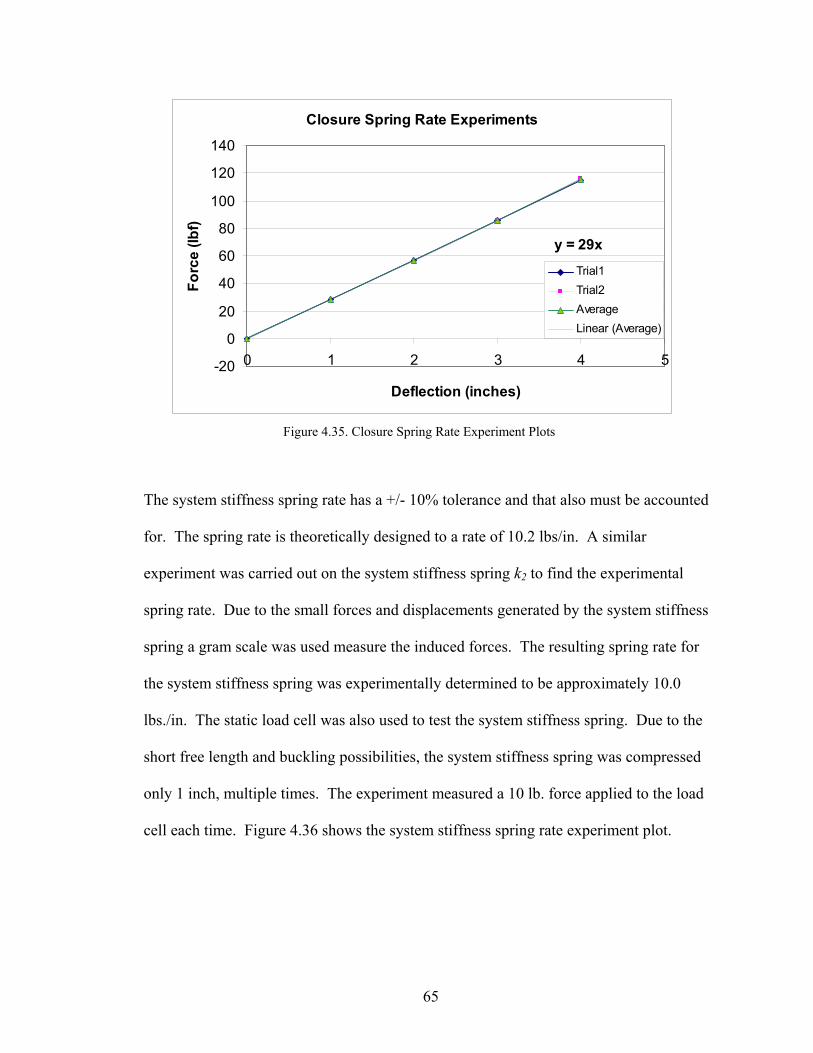
65

The system stiffness spring rate has a +/- 10% tolerance and that also must be accounted

for. The spring rate is theoretically designed to a rate of 10.2 lbs/in. A similar

experiment was carried out on the system stiffness spring k2 to find the experimental

spring rate. Due to the small forces and displacements generated by the system stiffness

spring a gram scale was used measure the induced forces. The resulting spring rate for

the system stiffness spring was experimentally determined to be approximately 10.0

lbs./in. The static load cell was also used to test the system stiffness spring. Due to the

short free length and buckling possibilities, the system stiffness spring was compressed

only 1 inch, multiple times. The experiment measured a 10 lb. force applied to the load

cell each time. Figure 4.36 shows the system stiffness spring rate experiment plot.

Figure 4.35. Closure Spring Rate Experiment Plots

Closure Spring Rate Experiments

y = 29x

-20

0

20

40

60

80

100

120

140

0 1 2 3 4 5

Deflection (inches)

Forc

e (lb

f)

Trial1Trial2AverageLinear (Average)

66

Using the experimental data for the physical parts, the calculations for the natural

frequencies of the two-DOF lumped mass model were redone. The same Mathcad sheet

was used to calculate the measured natural frequency of the system. The theoretical

values of the lumped mass m1 and closure spring rate k1 were changed to the actual

masses of the parts and the actual spring rate of the closure spring. The mass m2 block

was also weighed; its mass was the same as the theoretical value. Appendix E contains

the Mathcad worksheet used to calculate the physical system properties. The new lower

natural frequency of the system when split into two-DOF is 178 rpm and the upper

natural frequency is 446 rpm.

The increase in the closure spring rate, from 27 to 29 lbs./inch and the decrease in

mass m1, from 0.0193 bl to 0.0192 bl makes the natural frequency a higher value than

calculated. The higher natural frequency required the fixture to be run faster. The

calculated top speed of the cam test fixture is about 300 rpm using the maximum speed of

the motor and the pulley ratio. Any test speed less than 300 rpm is acceptable. The

physical system is run at 178 rpm, which is well below the limits of the test equipment.

Figure 4.36. System Stiffness Spring Rate Experiment Plots

67

4.10 Stress Analysis of Follower System

A detailed stress analysis of

the follower system, using TK

Solver, was carried out to calculate a

factor of safety for the follower shaft

under the loading from the cam and

return spring. Figure 4.37 shows the

force and pressure angle diagrams

for calculating the cam-follower

contact force. The component of the

Normal force N acting perpendicular

to the follower motion acts to bend

the follower shaft and jam it in the

bushings. The induced stresses in the shaft must be calculated due to this force.

The follower shaft in its assembled state can be modeled as a beam with an

overhung load being applied by the cam. Figure 4.38 shows the loading diagram for an

overhung beam with a concentrated load. The supports are created by the two grounded

bushings in the fixture frame, one located close to the roller and the other close to m2.

Figure 4.37 Press. Angle and Contact Force Diagram

Figure 4.38. Overhung Beam Model of Follower Shaft

68

The assumption of using an overhung beam model implies that the bushings are

point supports and the beam is left free to bend between them. This is a good assumption

because the follower shaft will have some deflection due to tolerances during the

assembly of the shaft into the bearings. The follower shaft must be allowed to have some

motion in the bushings to keep it from locking up. If the follower shaft becomes locked

up, then the force acting transversely to the shaft can cause it to bend and eventually fail.

If the follower shaft gets locked in the bushing, it is analogous to a cantilevered beam

under concentrated loading, for one end is fixed and the other is free to bend under the

loading. If the slope of the shaft deflection under loading is smaller than the angle

created by the gap of the shaft and bushing, this cantilever effect will not happen.

The follower shaft is comprised of three separate sections welded together,

creating a non-uniform cross section for the beam. The equations for deflection and

stress cannot be taken directly for a simple beam. Stress concentrations and the changing

moment of inertia of the separate sections must be accounted for. A TK Solver program

written by R.L. Norton was modified to create the forces and stresses from the

Figure 4.39. Bending Stress vs. Cam Angle

69

component of the cam contact force that is perpendicular to the follower motion. The

program was rewritten twice; the first modification uses lists to plot out the maximum

stresses in the follower shaft throughout the entire 360 degrees of cam rotation. Figure

4.39 (previous page) shows the max bending stresses in the follower shaft over the entire

cam rotation. This program also calculates the deflections that the follower shaft

undergoes during a complete rotation of the cam. When deflected, the shaft effectively

bows out convexly, so there will be a maximum and a minimum value of deflection,

measured from the y-axis, for each rotation angle of the cam. Figure 4.40, shows the

maximum and minimum deflections of the follower shaft for 360 degrees of cam rotation.

The second program uses similar lists with variables used to calculate the beam

profile for any position of the cam. The maximum stress and deflection both occur at 202

degrees of cam rotation. Using the second program and using 202 as the list variable the

maximum bending stresses can be calculated. The follower shaft, under the loading of

Figure 4.40. Deflection vs. Cam Angle

0 50 100 150 200 250 300 350 400-.01

-.008

-.006

-.004

-.002

0

.002

.004

.006

.008Max/Min Deflection vs. Cam Angle

Cam Angle, theta (degrees)

Defle

ctio

n (in

ches

)

Maximum Deflections

Minimum Deflections

70

the preload from the closure spring, plus the dynamic forces has a maximum bending

stress of 5,278 psi. This value is at the bushing support located at the cam interface end

of the follower shaft and is on the solid 3/4-inch diameter shaft section. The induced

stress is much lower than 77 kpsi, the tensile yield stress of the SAE 1045 cold drawn

steel of which the shaft is made; a safety factor of 13.44 in bending results. This program

also calculates the deflections of the follower shaft at any given position of the cam.

Figure 4.41, shows the deflection at cam angle 202 degrees.

The location of the maximum deflection of the beam is between the two bushing

supports. The maximum deflection at the cam interface, where the loading is applied, is

about 0.004 inches. The deflection and stress calculations have to be carried out for

every position of the cam angle due to the fact that the pressure angle and dynamic force

change with each step of cam rotation. These values were used to calculate the force

component applied perpendicular to the follower shaft. Appendix F contains the TK

Solver files that calculate the stresses and deflections of the follower shaft.

Figure 4.41. Deflection Diagram for Position 202 degrees Cam Rotation

71

5.0 Data Collection

The data collected are experimental time and frequency responses from the two

accelerometers mounted on the moving parts of the follower train as well as the time

responses of the two LVDT’s mounted to the follower train. The method of tracking the

camshaft angular velocity was to connect a Hewlett Packard universal counter to the

1024 counts per revolution shaft encoder that is mounted to the flywheel end of the

camshaft. The counter will give an accurate count of the number of lines it reads per

second. This value can be easily converted to the angular velocity in Hz by dividing the

counter reading by the 1024-encoder lines. Multiplying by 60 gives the angular velocity

in rpm.

5.1 Dynamic Signal Analyzer

An Agilent Technologies 36070A Dynamic Signal Analyzer was chosen for this

research, Figure 5.1. The analyzer has four input channels and can be triggered

externally or can be allowed to

“free-run” while taking data. The

four channels were used to capture

data traces from the two

accelerometers and the two

LVDT’s mounted to the testing

apparatus. The signals from the

two accelerometers are fed into a

power supply and then into the first two channels of the analyzer, through BNC cables.

Figure 5.1. Dynamic Signal Analyzer

72

The two LVDT’s were wired into a +/- 15 Volt DC power supply and then connected to

the analyzer using two more BNC cables.

By having four channels operating on the analyzer, a total resolution for each

channel of 800 lines in the frequency domain was obtained, corresponding to a 2048 line

resolution in the time domain. When running tests the channels must be set up for the

time or frequency span in which the operator would like to take data. The operator can

only set the frequency span, which in turn sets the time domain. A short frequency

window relates to a large time window and a large frequency window relates to a short

time window. For instance a 100 Hz frequency span relates to an 8 second window in the

time domain and a 1600 Hz frequency span creates a 0.5 second time window.

The resolution and window spans are important when taking data traces. The

delta segments between data points are governed by the span and resolution. For this

reason, two traces are usually taken; one with a window to allow an accurate time trace

and one with a window that allows an accurate frequency spectrum. For instance, if a

large time window is selected, then the delta t becomes very large and the delta f

becomes very short, giving very good results in the frequency domain but not in the time

domain. The delta units need to be taken into account when capturing data.

The analyzer is also able to take a set number of averages of data and then present

those results to the operator, which can be helpful to remove any random noise picked up,

such as another machine turning on. When investigating an event that occurs over a very

short time period it is often better to take a single screen shot to record the data. Single

shots allow the operator to control what data are recorded. If the event is missed the

operator can easily erase the data and keep recording until the event is captured.

73

5.2 Experimental Procedure

The experimental procedure was to run the cam test fixture up to a speed close to

the design speed of 178 rpm, which is equal to the first post-separation mode natural

frequency as computed in the model. According to the dynamic model, the system

should jump its follower at that speed. The test cam chosen was an old, milled cam with

wear and pitting on its surface. The cam and follower will stay in contact provided there

is enough preload force being supplied by the closure spring. The test fixture has a

preload adjustment mechanism incorporated into the design. The protocol was to run the

system up to the jump speed with the preload screw at its maximum extension, creating

the maximum amount of preload force, about 82 lbs. While running at the jump speed,

with the extra preload preventing jump, accelerometer data were recorded in both the

time and frequency domains. LVDT time traces were also recorded. Keeping the

camshaft speed settings constant, the preload screw was slowly backed out, decreasing

the preload force until the system began to jump slightly. Data were again taken during

this mode. The preload screw was further backed out until the system was violently

jumping and data were taken during this mode. Since data were collected during the

period when the system was jumping and coming back together the signal trace should

show the frequencies for both the in-contact case and the separated case.

The data collection method was the same for all measurements. The

accelerometer and LVDT responses were input to a dynamic signal analyzer to examine

the values in both the time and frequency domains. A once-per-revolution shaft encoder

mounted to the camshaft was used as a trigger for all measurements taken. The machine

was run at approximately 182 rpm and the frequency span was set at 100 Hz. The 100

74

Hz span created an 8 second data collection time, which was considered suitable for this

experiment and was used to capture the frequency responses for both accelerometers.

The frequency span was then changed to 1.6 kHz and the time traces were again taken for

both accelerometers. At 1.6 kHz, the time window was at 0.5 seconds. The LVDT data

were taken with an 800 Hz frequency span, corresponding to a 1 second time window,

which allowed three rotations of the cam to be captured during the data collection.

Mr. Ernest Chandler of The Gillette Company took high-speed video of the test

fixture at the jump speed. The camera captured video at a rate of 500 frames per second.

Video was recorded of the test fixture running with both jump and no jump conditions.

These data were used to calculate the separation time and to scale the separation distance.

Calculations were conducted using the equations for the natural frequencies of the

two-mass two-DOF dynamic model. The natural frequency equations were used to see

what effect changing the system parameters or design variables would have on the

resulting natural frequencies. There are four parameters in the natural frequency

equation, m1, m2, k1, and k2. The theoretical calculation protocol was simple; adjust the

different design variables to see what their effect was on the SDOF and both two-DOF

system natural frequencies. The system stiffness spring rate k2 value was increased to

10,000 lb/in., which is a more realistic value for the stiffness of a follower train. With

this high value in place, the m1, m2, and k1 values were modified and the natural

frequencies were recalculated. These are the three experimental protocols used in the

data collection.

75

6.0 Results

When the system begins to jump, the camshaft speeds up due to reduced load on

the motor. The camshaft speed does not stay constant even with the large flywheel.

During the tests, the camshaft speed fluctuated, sometimes up to 4 rpm. The motor speed

is regulated through a DC speed controller, meaning the operator can dial in how much

current is going to the motor. The current supplied to the motor is related to the output

speed. This type of motor controller is inaccurate for fine speed control. To account for

phase shifts in the data due to speed changes, order analysis was used. The independent

variable is normalized by the average speed of the camshaft. The unit of frequency then

becomes harmonic number. For the time traces the independent variable is divided by

the period of the camshaft revolution, the time units then become revolutions.

The three modes in which data were recorded are the response of the system

before it jumps, when the system is slightly jumping and when the system is violently

jumping. Mode 1 describes the situation when the system is at the jump speed, but not

jumping, due to sufficient preload. With the added preload from the adjustment screw,

the system stays in contact even at the designed jump speed. Mode 2 describes the period

when the preload screw is backed out and the system begins to slightly jump. While in

this mode the system jumps once or twice per recorded cycle. Mode 3 describes the

period in which the preload screw has been backed out enough to reduce the preload to

allow the system to violently jump. During this mode the system jumps every revolution

in the recorded cycle. This terminology will be used throughout the discussion of the

results and conclusions.

76

6.1. High Speed Video The results of the high speed (HS) video show that the system was in fact jumping

the follower during the fall portions of the cam program. Figure 6.1 shows a still frame

of the system just as it starts on the fall period. The cam and follower remain in contact

through the high dwell portion of the cam cycle.

Figure 6.2 captures a frame where the cam and follower have physically separated.

During the fall, the cam follower acceleration function exceeds the actual acceleration of

the physical follower, pulling the cam surface out from under the roller. The roller

follower has a 2-inch outer diameter (OD). Using the OD as a reference the separation

distance can be scaled approximately to be in the tenths of an inch range. Using the HS

video playback information the separation time can be evaluated at about 0.012 seconds.

Figure 6.1. HS Video Frame Prior to Jumping

Roller Follower

Cam

77

The closure spring is still pushing downward on the follower train due to its compressed

state, even though it is uncompressing on the fall and there is no contact between the cam

and follower. Eventually the follower and cam will regain contact with an impact.

Figure 6.3 shows a still frame captured directly after the cam and follower regain contact.

Figure 6.2. HS Video Frame During Follower Jump

Roller Follower

Cam

Figure 6.3. HS Video Frame After Cam-Follower Return

Roller Follower

Cam

78

6.2 Time Response

The LVDT results of one revolution for the three operational modes for mass m1

can be seen in Figure 6.4. The mass m1 LVDT data closely match the displacement curve

created in Dynacam.

There is very little discernable change in the data traces among the three operational

modes in Figure 6.4. This indicates that the response time of the LVDT is not fast

enough to capture the jump phenomenon. The total separation distance between the cam

and follower is estimated to be in the tenths of an inch range. Figure 6.2 (page 67) shows

the follower jump to start at the beginning of the fall event. The cam and follower then

regain contact approximately midway through the fall period. At the fixture’s running

speed, this is a very short length of time. From the HS video the separation time can be

Figure 6.4. Mass m1 LVDT Data for Three Operational Modes (1 revolution)

79

measured as 0.012 seconds. It is difficult in the analyzer to capture a phenomenon with

extremely small magnitude that happens in a short period of time because of the

recording resolution.

Interesting results are revealed in the time trace for the LVDT that was mounted

to the output mass m2 block. Figure 6.5 shows the time data for the mass m2 LVDT.

The magnitudes of the displacement are increasing in magnitude through the different

modes. Mode 1 has smaller magnitudes when compared with those of Mode 2 and then

Mode 3.

Figure 6.5. Mass m2 LVDT Data for All Three Operational Modes

80

The oscillation pattern is evidence of the different functions used in the creation

of the cam program. The program is made up of two rise and two fall events. Each event

is created with a different acceleration function. The output mass is loosely coupled to

the follower train through a 10 lb/in. compression spring. During the dwell portions of

the cam program, the output mass over travels the event and does not dwell when run at

sufficiently high speeds. In Figure 6.5 each peak value of displacement, whether high or

low, is consistent with a dwell segment of the cam. The higher magnitude acceleration

functions create stronger oscillations in the displacement of the output mass. Thus if the

event has a higher peak acceleration it will take more travel (displacement) to slow the

mass down during the cam’s dwell segment. The over travel creates a higher peak

displacement in the output mass’s motion.

Figure 6.6 shows the time traces for the mass m1 accelerometer in all three modes.

-10000

0

10000

20000

30000

40000

50000

0.0 0.2 0.4 0.6 0.8 1.0 1.2 1.4

Revolutions

Acce

lera

tion

(in/s

^2)

Mode 1-Prejump

Mode 2-Slight Jump

Mode 3-Violent Jump

Mass m1 Acceleration in Three Modes

Figure 6.6. Mass m1 Acceleration for All Three Modes

81

One can clearly see the jump phenomenon in the mass m1 accelerometer data. Large

acceleration responses are seen in the time data when the cam and follower impact after a

jump and return event. The time traces shown were taken as single screen shots on the

signal analyzer to ensure a jump and return event was recorded.

In Figure 6.6, one and a half revolutions and thus three jump / return events are

shown. There are two rise-dwell-fall events per cam rotation. Mode 2 has only one jump

spike located at the second revolution and is of moderate amplitude. Mode 3 has the cam

and follower jumping on every rotation. These are clearly indicated by the large

acceleration spike amplitudes upwards of 50,000 in/s2 associated with impact. The

acceleration magnitudes in Mode 1 match closely to the theoretically calculated follower

accelerations in Dynacam.

Figure 6.7 shows the mass m2 time response for all three modes.

Figure 6.7. Mass m2 Acceleration for All Three Modes

Mass2 Acceleration in Three Modes

-4000

-3000

-2000

-1000

0

1000

0.000 0.200 0.400 0.600 0.800 1.000 1.200 1.400

Revolutions

Acce

lera

tion

(in/s

^2)

Mode 1-Prejump

Mode 2-Slight Jump

Mode 3-Violent Jump

Mass m2 Acceleration in Three Modes

82

With each jump phenomenon occurring at the cam-follower interface, corresponding

spikes of increased acceleration occur in the time trace of mass m2. The mass m2 jump

phenomenon in Mode 3 happens once per revolution following the same pattern as in the

mass m1 data. Again, Mode 2 only has one jump spike showing up at the second

revolution. The mass m2 accelerometer time data correlate well with the mass m1 data.

The two data sets have one jump phenomenon recorded at the second revolution during

Mode 2, and have jump spikes recorded at every revolution during the Mode 3 stage.

Mode 1 prejump data from both accelerometers gave expected results.

6.3 Frequency Response

The frequency data were taken with an operating speed of approximately 182

rpm, or about 3 Hz. The designed natural frequencies are 4.32 Hz for the SDOF case,

and 2.95 Hz and 7.94 Hz for the two-DOF case. The SDOF natural frequency should not

show up during the prejump stage, while running at 182 rpm or 3 Hz (two-DOF natural

frequency), because there is adequate preload force to keep the cam and follower together

at all times. The SDOF system does not resonate as long as contact between cam and

follower is maintained and the system is not run at its natural frequency of 4.32 Hz.

According to the untuned vibration

absorber frequency plot (Figure 6.8),

the SDOF natural frequency may

show up in the two-DOF mode when

the follower is jumping.

Figure 6.8. Frequency Response SDOF System

SDOF Frequency

83

Two things are looked for in the frequency response. The first is whether or not the

system switched to the two-DOF mode. The two-DOF system switch can be seen if the

two-DOF natural frequencies show up in the spectrum. The second is whether the natural

frequencies of the two-DOF system grow in amplitude when the system is jumping.

When taking the frequency data it is especially important to remember the

limitations associated with resolution and frequency span issues. All the frequency data

were taken at a 100 Hz span in an 8-second time window with 2048 data points, which

means the delta time is 0.004 seconds. This resolution is poor for this application and

does not allow the operator to get a good time image when the system is slightly jumping

(Mode 2). The jump/return spikes are essentially instantaneous and can be considered

impulses. The analyzer can easily miss the event being investigated with the given delta

time. Through experiment, it was found that in Mode 2 it was impossible to record a time

trace that showed the jump phenomenon with that time window. The acceleration events

associated with Mode 2 are easily seen with a small time window and a smaller delta

time. The downside to having a small time window is that the resolution in the frequency

domain becomes so poor that the frequency data become meaningless.

The frequency data needed to be normalized due to minor fluctuations in camshaft

speed. To make the data comparable, order analysis was conducted. The frequency

response was divided by the average camshaft speed in Hz. This calculation results in the

normalized unit of harmonic number or order. Equation 6.1 is used to calculate the

harmonic numbers:

(6.1)

84

Table 6.1 shows the calculated order numbers and their amplitudes corresponding

to the natural frequencies being investigated. The average camshaft angular velocity for

each mode is also presented.

To capture the system information completely, the operator needs both a time

trace and a frequency spectrum of the device being investigated. Cam functions typically

have high harmonic content. When looking at the frequency domain of a cam-follower

acceleration function, many peaks show up in its spectrum. The dynamic signal analyzer

calculates the Fast Fourier Transform (FFT) and presents the resulting data in the

frequency domain. When capturing the frequency domain data, the analyzer also

captures the harmonic content of the cam system. If a cam has particularly high

harmonic content compared to the events being investigated, these events can be masked

as noise. Figure 6.9 shows the magnitudes and harmonic numbers of the FFT for the test

cam as calculated in Dynacam.

Figure 6.9. Test Cam Acceleration FFT (Cam Harmonics)

Table 6.1. Order Analysis Results

Frequency Order Prejump Slight Violent(Mode 1) (Mode 2) (Mode 3)

2DOF Low 2.95 Hz 0.96 10 13 251DOF 4.32 Hz 1.41 0.5 5 102DOF High 7.44 Hz 2.42 2 5 10

ωave 182 rpm 184 rpm 184 rpm

Amplitudes (in/s^2)

85

As one can see in Figure 6.9, this particular test cam has very strong 2nd, 6th, and 10th

harmonics. The 8th and 12th harmonics also have substantial peaks but are significantly

lower than the 6th harmonic which dominates the frequency spectrum for this cam

acceleration function. The test cam has two rise-dwell-fall-dwell events, which creates a

strong second harmonic. It is this double “hump” cam profile that is responsible for

creating the even harmonic distribution in the theoretical FFT of the acceleration function

for the test cam. A single rise-dwell-fall-dwell program would lead to harmonics 1, 3,

and 5 being present instead of 2, 6, and 10.

The system harmonics show up in the frequency response when experimentally

taking accelerometer data. The data recorded from both mass m1 and mass m2 contain the

cam harmonics, and they are larger in magnitude when compared to the other events in

the frequency spectrum. It is important to observe that the cam harmonics are

consistently large in the experimental data spectrum similar to the theoretical FFT.

Figure 6.10 shows the frequency response for the mass m1 accelerometer.

Figure 6.10. Mass m1 Frequency Response (100 Hz Span)

86

The large 2nd and 10th harmonic peaks from the cam and the even larger 6th harmonic

peak are shown clearly in the spectrum. The operating speed is around 3 Hz and each

one of these large peaks is an integer multiple of that value, creating the harmonic content

of the cam. The actual harmonic content of a “realistic” cam is important to note in this

study. The typical cams used in industrial applications will contain high harmonic

content due to the functions used to create the cam program. Table 6.1 shows that the

frequencies being investigated are all less than 10 Hz and the associated amplitudes are

well within 50 in/s2. These values were used to box in and enlarge the data being

explored to make the natural frequencies visible.

Figure 6.11 is an enlarged view of Figure 6.10, zoomed into the region described

above and normalized to the order domain.

Figure 6.11. Enlarged View Mass m1 Harmonic Numbers

87

Shown enlarged, the Mode 2 frequency response is very similar to the Mode 1 data trace.

This similarity is due to the resolution issues discussed previously. The delta t in the

time window of 8 seconds was too large for the analyzer to pick up the jump

phenomenon. This results in the two plots being very similar. The amplitude of the 0.96

order is increased in Mode 3 over that of Modes 1 and 2. The increase in amplitude is

due to the switch to the two-DOF system condition. An acceleration spike shows up at

the 2.44 order as well. This acceleration spike is located at the higher of the two post-

separation mode natural frequencies. According to the system equations, when the

follower jumps and switches to two-DOF, the SDOF system natural frequency will split

into two lower amplitude values. Figure 6.11 shows both of these new system natural

frequencies showing up in the frequency response. The SDOF natural frequency also

shows up in frequency response at the 1.41 order.

The peaks due to the harmonics of the cam are much greater in amplitude than the

phenomenon that is being investigated. In Figure 6.11 it is easy to see the 2nd harmonic is

dominating the plot. The amplitude of the 2nd harmonic must be clipped at 50 in/s2, to

reduce the vertical scale. This truncation is done so the peaks of the natural frequencies

being investigated can be seen in the plot. The frequency amplitudes being looked at are

all below 20 in/s2. When the plot is shown in full scale, the amplitudes of the frequencies

in question are lost in the noise compared to the large amplitudes due to the cam

harmonics. After the data has been truncated at a maximum peak of 50 in/s2, the natural

frequencies that are being investigated show up clearly in the data plots.

88

The mass m2 acceleration shows similar responses in the frequency spectrum to

those of mass m1. Figure 6.12 shows the frequency response of the mass m2

accelerometer over a 100 Hz frequency span.

The cam harmonics dominate this spectrum similar to the mass m1 case. The mass m2

second harmonic has the greatest magnitude followed by the sixth harmonic.

Figure 6.13 is an enlarged view of the mass m2 frequency response, zoomed into

the region being investigated.

Figure 6.12. Mass m2 Frequency Response in Hz (100 Hz Span)

89

Only the lower of the two-DOF mode natural frequencies shows up in this response.

Both Mode 2 and Mode 3 show the first post separation mode natural frequency in the

spectrum. The 0.96 order shows up in both spectra. A peak located close to the 0.96

order shows up in the Mode 1 data. The operating speed and the two-DOF natural

frequency are essentially the same value. The operating speed is the value showing up in

the frequency response for Mode 1. The more valuable information gained from this plot

is that Mode 2 and Mode 3 both have the amplitude of the 0.96 order increasing, which is

what would be expected if the system were to switch to the two-DOF mode.

At 2.44 order the three plots are essentially the same. The higher natural

frequency of the two post separation modes does not show up in this plot, which is

surprising. This is hypothesized to be due to the resolution problems that were occurring

with the Mode 2 data. Only one two-DOF system natural frequency showed up in the

mass m2 data but both frequencies showed up in the mass m1 recorded data.

Figure 6.13. Enlarged View Mass m2 Harmonic Number

90

6.4 Natural Frequency Calculation Results

When examining an assembly machine, the parts of the follower train are usually

very stiff to keep tight tolerances for accuracy of product. Generally, this results in a

large system stiffness k2. If the system stiffness k2 is designed to be high, the SDOF

natural frequency and the lower of the two-post separation natural frequencies of the two-

DOF system will be very close to each other. The values of these two natural frequencies

can be as close as a fraction of 1 rpm. These two frequencies can then be represented by

a single value that should be used to design the operating speed. The operating speed

should be much less than the system natural frequency to avoid resonance.

The following paragraph contains tables of the calculated natural frequencies

along with the design variables used in the equations. Each variable has been increased

to see what the resulting effect is on the natural frequencies.

The follower variables used in the design of the test apparatus created a plot

similar to the untuned vibration absorber. These values can be seen in Table 6.2. Note 1

blob is equal to 1 (lbf-s2) / inch.

The opening paragraph states that with a sufficiently stiff follower train the SDOF

and the lower of the two post separation natural frequencies become very close. To

illustrate this fact see Table 6.3. Changing the system stiffness k2 value to a more

realistically large number places the two natural frequencies very close.

K1 (lb/in) m1 (blob) K2 (lb/in) m2 (blob)27 0.0193 10.2 0.02

SDOF (rpm) Two-DOF (rpm) Two-DOF (rpm)250.298 176.13 437.319

Table 6.2. Design Variables and Resulting Frequencies

91

The values in Table 6.3 are essentially the same, being separated only by 0.088 rpm or

0.035%. The more interesting results are obtained when modifying the other design

variables while keeping the system stiffness k2 at a realistic value. Keeping the system

stiffness k2 at a more realistic value creates a more accurate estimate of what would

happen in a real system.

If a particular design calls for a higher closure spring k1 preload value, one

solution would be to increase the closure spring k1‘s spring rate. If the closure spring k1’s

rate is increased, while the system stiffness k2 is still very high, then the SDOF and the

first post separation natural frequencies become extremely close in value. Table 6.4

shows the variables and the resulting natural frequencies.

In this case the values are different by a value of about 1.5 rpm or 0.25%. There is

always a tolerance with any calculation that is made. For this cam-follower system these

two values can be represented as 680 rpm, which can be used when comparing the

operating speed of the machine to the first natural frequency of the system.

Table 6.4. Increased k1 Value and Results

K1 (lb/in) m1 (blob) K2 (lb/in) m2 (blob)200 0.0193 10000 0.02

SDOF (rpm) Two-DOF (rpm) Two-DOF (rpm)681.224 679.458 9661

K1 (lb/in) m1 (blob) K2 (lb/in) m2 (blob)27 0.0193 10000 0.02

SDOF (rpm) Two-DOF (rpm) Two-DOF (rpm)250.298 250.21 9639

Table 6.3. Increased k2 Value and Resulting Frequencies

92

Some follower components can get rather large and heavy depending on what the

system is doing in the machine. If the designer creates a system with a large value for the

mass m1 follower train, the two natural frequencies in question calculate to the same

value. The results can be seen in Table 6.5.

Here the values become essentially the same, only off by 0.001%, and must be designed

around when creating the output speeds of the machine.

Some end effectors have considerable amounts of mass associated with them

depending on the operation being controlled by the cam-follower mechanism. For

example, if the end effector is holding a part with a robotic gripper, the end effector could

become very large. The size corresponds with the weight and the mass of the part. If the

end effector mass m2 is created with a large value, then the two values become essentially

the same once again, only being off by 0.08%, see Table 6.6.

There is one difference in this case, if the closure spring value k1 is also increased, then

the two natural frequencies in question begin to split like the vibration absorber. For

lower values such as 20 lb/in. the natural frequencies again come to extremely close

K1 (lb/in) m1 (blob) K2 (lb/in) m2 (blob)20 0.196 10000 0.02

SDOF (rpm) Two-DOF (rpm) Two-DOF (rpm)91.888 91.887 7089

Table 6.5. Increased m1 Value and Results

K1 (lb/in) m1 (blob) K2 (lb/in) m2 (blob)20 0.0193 10000 0.2

SDOF (rpm) Two-DOF (rpm) Two-DOF (rpm)91.194 91.118 7204

Table 6.6. Increased m2 Value and Results

93

values. Appendix H shows the theoretical variations and the solutions that were

calculated.

94

7.0 Conclusions

This section contains conclusions drawn based on the results of both the

experimental tests and the theoretical calculations. It is good to note that what the theory

predicts does actually transpire. For instance, while the system is jumping, the time

response of the mass m1 accelerometer shows large amplitude spikes of acceleration

when the system is impacting. These large spikes are located at the positions of the falls

of the cam displacement function, corresponding to what the literature states. Periods of

high negative acceleration, such as steep falls, generally are where follower jump occurs.

Any body when excited and left to vibrate freely will resonate at its natural

frequency. Vibration at resonance is easily seen with a simple tuning fork or a bell.

When the tines of the tuning fork are impacted the fork will vibrate at its natural

frequency. Similarly when a bell is struck it will ring at its natural frequency. Likewise

any machined part when struck will ring at its natural frequency. When a cam-follower

system jumps it then becomes free to resonate at its natural frequencies. The test fixture

follower train vibrating at its natural frequencies was shown in the resulting experimental

data traces. When the system jumped it switched to the two-DOF mode and had its new

natural frequencies show up in the frequency spectrum.

7.1 Experimental System Conclusions

The collection of the Mode 2 or slightly jumping case data was stricken with

recording problems due to the resolution issues with the dynamic signal analyzer. The

experimental procedure being followed used the preload adjustment screw to reduce the

closure spring k2‘s preload while the system was running at the designed jump speed.

95

Running at the jump speed with marginal closure spring k1 preload creates the incipient

state where the system would be ready for follower jump. The cam chosen had a rough

surface finish with wear present. Having the preload set at the cusp of separation and a

cam with a poor contact surface was the ideal setup for this experiment. However, during

Mode 2 no frequency responses could be recorded with a high enough resolution to see

any of the slight jumps the cam and follower were experiencing. The time data did show

the system was indeed jumping by the large acceleration spikes present in the trace. By

not capturing any of the jump events in the frequency spectrum, the two-DOF natural

frequencies could not be investigated. The data that showed the more interesting results

were during Mode 3 or when the cam and follower were violently jumping. Mode 3 is a

direct result of reducing the preload until there is physically not enough force to keep the

cam and follower in contact. The results of the Mode 3 case prove that the system does

switch to the two-DOF mode by capturing the natural frequencies in the spectrum.

It can be concluded that the system does switch to the two-DOF mode when the

system jumps as theoretically predicted. The theory states that when a cam and follower

mechanism loses contact the follower is free to resonate. If the system under study,

behaves like a two-mass dynamic model (which most linkage systems will) then the

system will have two coupled natural frequencies. These can be seen in the results where

the natural frequencies of the two-DOF system show up in the frequency response of the

mass m1 accelerometer. Furthermore, the phenomenon that was being searched for exists

and is measurable with the proper instrumentation. The time traces on the signal analyzer

showed that the system was indeed jumping, due to the large acceleration peaks at the

cam-follower return. The jump condition was also supported by the high-speed video

96

recorded of the follower system when run at the design speed. The frequency data was

then collected to search for the natural frequency peaks.

The major conclusions to this research are that in a practical aspect this

phenomenon of the system switching to the two-DOF mode will not have a major effect

on the dynamic response of the follower system. The test cam used has a somewhat

complicated program, similar to a typical assembly machine cam. The program was

created with four different cam functions and contains eight separate events. This type of

program is common in cams used in production machinery. Having the complicated

programs and a multitude of functions used in the design of the cam creates high

harmonic content. The test cam has similar high harmonic content as discussed above.

The amplitudes of the cam harmonics dominate the spectrum, placing the peaks of the

two-DOF natural frequencies close to zero on the vertical axis, towards the noise level of

the trace. The energy due to the two-DOF switch compared with the total energy of the

cycle of the cam is extremely small. The significance of the vibrations caused by the

two-DOF natural frequencies becomes low, which minimizes their influence in the

follower’s output motions.

The actual jump and return events will still have an extreme effect on the output

motions of the cam-follower system. During the experimentation, Mode 2 jumps were

difficult to capture on the analyzer even in the time domain. When the acceleration

spikes were captured the magnitude was only about half that of the Mode 3 magnitudes.

The return crashes are significant causes of vibration but the frequencies corresponding

with the two-DOF system switch are not. The Mode 3 violent jumping phenomenon had

extremely large impact acceleration magnitudes, which clearly will cause vibration issues

97

in high-speed machinery. It is clearly seen that both the time data and the frequency

response are needed to analyze a system thoroughly enough to generate conclusions.

7.2 Natural Frequency Calculation Conclusions

The natural frequency calculations show that if the machine in question has been

designed for good dynamic performance, i.e., the follower train is created very stiff, then

the two natural frequencies (SDOF and lower two-DOF mode) will be extremely close in

value. When designing a new cam-follower mechanism, the designer usually has good

information on the masses and stiffness of the parts in the design. 3D CAD modeling

makes this very easy to calculate. If the designer takes the values into account, they will

be able to calculate a good approximation of the first natural frequency of the system.

The operating speed is usually specified by management. If the required operating speed

is close to the calculated natural frequency then the station may need to be redesigned to

accommodate the required speed. The speed dictates the way in which the machine will

be designed.

If the theoretical calculations are correct, for a stiff follower, even if the system

were to jump due to poor cam surface quality and preload force, the system would never

be running near the lower of the two-DOF natural frequencies. The lower of the two-

DOF frequencies is essentially equal to the SDOF natural frequency, which would

already be estimated for the machine. The conclusion of this theoretical work is that the

system simultaneously switching to the two-DOF mode and resonating will not happen in

reality. The ratio of the stiffnesses of k1 (closure spring rate) and k2 (the greater follower

system stiffness common in industrial production machinery), forces the SDOF and the

98

lower of the two post separation natural frequencies to be close together. The machine

should never be run near its SDOF natural frequency. The lower of the two-DOF natural

frequencies will then also be above the operating speed. Then the system should not

switch to the two-DOF mode and resonate.

99

8.0 Recommendations

The recommendations being presented discuss the benefits of dynamic modeling

of cam-follower systems before the actual building and assembly of the device. Some

design parameters have certain characteristics that lead to a well-designed system. These

need to be followed when designing cam-follower mechanisms.

• When designing a new station on a production machine that includes a cam and

follower mechanism, it is extremely important to create the follower train as stiff

as possible. High stiffness can be accomplished by using beams with high cross

sectional area moments of inertia, not by making everything bigger. Designing

large follower systems is not a feasible solution. Ideally the parts in the follower

train should have high specific stiffness values. Creating large parts does not

increase the specific stiffness; it can actually lower it because the mass is

increased. By creating a highly stiff follower train the natural frequencies of the

SDOF and the first post separation two-DOF mode will be essentially identical.

Being a responsible engineer, the designer would design the natural frequencies of

the follower system to be significantly higher than the given operational speed.

• Analysis of a cam-follower design must be carried out before any prototype

machining and assembly. Dynamic modeling allows the system to be analyzed

prior to any material being cut. The mathematical model gives a good estimate of

how the system will behave when the system is run at similar conditions to the

design variables. The design of the follower train should be carried out using a

100

solid modeling CAD package. Using solid models allows 3-dimensional

assemblies to be created, calculation of the masses of parts, calculation of the

moments of inertia of parts, and the ability to see the assembly in motion on the

computer screen to debug any problems before it is built. Some 3D CAD

packages allow stress analysis to be carried out using FEA techniques.

Calculating the stresses on the follower train components pre-assembly can be

very useful to the designer. Calculating the stresses allows the design to be

modified before fabrication to prevent failure of parts.

• The first natural frequency must be calculated when designing a new cam-

follower mechanism. The first natural frequency is fundamentally important to

high-speed machinery, the operating speed must be much lower than the first

natural frequency of the follower system. The result, a better design, will

outweigh the initial costs of doing the analysis.

101

Bibliography Bagci, Cemil (Tennessee Technological Univ) & Kurnool, Srihari “Exact Response Analysis and Dynamic Design of Cam-Follower Systems Using Laplace Transforms” Source: American Society of Mechanical Engineers, Design Engineering Division (Publication) DE, Proceedings of the 1994 ASME Design Technical Conferences. Part 1 (of 2), Sep 11-14 1994, 1994, Minneapolis, MN, USA Sponsored by: , ASME ASME, New York, NY, USA, p 613-629 CODEN: AMEDEH Baratta, F.I., and J. I. Bluhm, “When Will a Cam Follower Jump.” Journal of Product Engineering, July 1954, pp. 156-159. Dresner, T.L. & Barkan, P., “New Methods for the Dynamic Analysis of Flexible Single-Input and Multi-Input Cam-Follower Systems” Source: Journal of Mechanical Design, Transactions Of the ASME, v117, n1, Mar, 1995 ASME, New York, NY, USA, p 150-155, ISSN: 1050-0472 CODEN: JMDEEC Dudley, W.M., “New Methods in Valve Cam Design.” Source: SAE Quarterly Transactions 1948, 2(1), pp. 19-33. Horeni, B. (State Textile Research Inst), “Double-Mass Model of an Elastic Cam Mechanism” Mechanism & Machine Theory, v 27, n 4, Jul, 1992, p 443-449, ISSN: 0374-1052 CODEN: MHMTAS Juvinall, Robert C. and Kurt M. Marshek, “Fundamentals of Machine Component Design.” Third Edition. John Wiley & Sons Inc. New York 2000. Kreyszig, Erwin. “Advanced Engineering Mathematics.” 8th edition, John Wiley and Sons, Inc. New York, 1999. Matsuda, T. (Shizuoka Univ) & Sato, M. “Dynamic Modeling of Cam and Follower System. Evaluation of One Degree of Freedom Model” Source: American Society of Mechanical Engineers, Design Engineering Division (Publication) DE, Vibration Analysis - Techniques and Applications, Sep 17-21 1989, 1989, Montreal, Que, Can Sponsored by: , ASME, Design Engineering Div, New York, NY, USA Publ by ASME, New York, NY, USA, p 79-84 CODEN: AMEDEH Mendez-Adriani, J.A., 1985. “Design of a General Cam-Follower Mechanical System Independent of the Effect of Jump Resonance,” ASME paper, 85-DEC-56. Merriam-Webster (2002). Merriam-Webster OnLine Dictionary-Thesaurus [Online]. Available: http://www.m-w.com/dictionary.htm Last accessed 5/14/02.

102

Norton, R. L. “The Cam Design and Manufacturing Handbook.” The Industrial Press, New York, 2002 Norton, R.L. “Machine Design- An Integrated Approach.” Second Edition, Prentice Hall, New Jersey, 2000 Raghavacharyulu, E. and J.S. Rao, “Jump Phenomena in Cam-Follower Systems a Continuous-Mass-Model Approach.” American Society of Mechanical Engineers, Proceedings of the Winter Annual Meeting, New York, NY, 1976, pp.1-8. Rao, Singiresu S. “Mechanical Vibrations.” Third Edition. Addison-Wesley Publishing Company, Reading MA 1995. R.C. Rosenberg & D.C. Karnopp, “A Definition of the Bond Graph Language” Transactions of the ASME. Journal of Dynamic Systems, Measurement and Control, September 1972, pp. 179-182 R.C. Rosenberg & D.C. Karnopp, “Introduction to Physical System Dynamics” McGraw Hill Inc., New York, 1983. Sadek, K.S.H. (Univ of Newcastle upon Tyne), Rosinski, J., & Smith, M.R., “Natural Frequencies of a Cam Mechanism.” Source: Proceedings of the Institution of Mechanical Engineers, Part C: Mechanical Engineering Science, v 204, n 4, 1990, p 255-261, ISSN: 0954-4062 CODEN: MESCEO Shigley, Joseph E. and Charles R. Mischke, “Mechanical Engineering Design.” Sixth Edition. McGraw Hill, New York, NY 2001. Siedlitz, S. (1989). “Valve Train Dynamics –A Computer Study” 890620, SAE. Tsay, D.M. (Natl Sun Yat-Sen Univ) & Huey, C.O. Jr. “Synthesis and Analysis of Cam-Follower Systems with Two Degrees of Freedom” Source: American Society of Mechanical Engineers, Design Engineering Division (Publication) DE, Advances in Design Automation - 1989, Sep 17-21 1989, 1989, Montreal, Que, Can Sponsored by: , ASME, Design Engineering Div, New York, NY, USA Publ by American Soc of Mechanical Engineers (ASME), New York, NY, USA, p 281-288 CODEN: AMEDEH Turgut Tumer, S. (Middle East Technical Univ) & Samim Unlusoy, Y., “Nondimensional Analysis of Jump Phenomenon in Force-Closed Cam Mechanisms” Source: Mechanism & Machine Theory, v 26, n 4, 1991, p 421-432, ISSN: 0374-1052 CODEN: MHMTAS