Virginia Commonwealth University Virginia Commonwealth University

VCU Scholars Compass VCU Scholars Compass

Theses and Dissertations Graduate School

1993

An Investigation of Bank Lending Practices To Test Portfolio An Investigation of Bank Lending Practices To Test Portfolio

Theory and Theories of Credit Rationing and Customer Theory and Theories of Credit Rationing and Customer

Relationships Relationships

Christine Chmura

Follow this and additional works at: https://scholarscompass.vcu.edu/etd

Part of the Business Commons

© The Author

Downloaded from Downloaded from https://scholarscompass.vcu.edu/etd/4419

This Dissertation is brought to you for free and open access by the Graduate School at VCU Scholars Compass. It has been accepted for inclusion in Theses and Dissertations by an authorized administrator of VCU Scholars Compass. For more information, please contact libcompass@vcu.edu.

School of Business

Virginia Commonwealth University

This is to certify that the dissertation prepared by Christine Chmura entitled

An Investigation of Bank Lending Practices To Test Portfolio Theory and

Theories of Credit Rationing and Customer Relationships has been approved by her committee as satisfactory completion of the dissertation requirement

for the degree of Doctor of Philosophy in Business.

Dr. Nei Di r

Dr. D e Member

Dr. Steven P. Peterson, Committee Member

Dr. Daniel Salandro, Committee Member

Dr. H

Dean, School of Business

� � !9P3 Date

An Investigation of Bank Lending Practices

To Test Portfolio Theory and

·""

Theories of Credit Rationing and Customer Relationships

A dissertation

submitted in partial fulfillment of the requirements for the

degree of

Doctor of Philosophy

at

Virginia Commonwealth University

By

Christine Chmura

M.A. Economics, Clemson University, 1983

B.A. Business Administration, 1981

Director: Neil B. Murphy,

Chairman,

Department of Finance and Insurance

Virginia Commonwealth University

Richmond, Virginia

December 1993

ct�Christine Chmura 1993 All Rights Reserved

ii

ACKNOWLEDGEMENTS

The author gratefully acknowledges the encouragement and support

provided by many individuals throughout the writing of this dissertation.

Special thanks is extended to the case study bank which provided the

database that made this study possible and to the many individuals within

the case study bank who graciously offered their time to explain the

database and to provide their views regarding commercial loan pricing.

Special thanks is also offered to ZETA® Services Incorporated and, in

particular, Constance Kenneally for providing credit scores by industry.

Finally, this study would not have been completed without the guidance and

support of my dissertation committee: Dr. Neil B. Murphy (Chairman). Dr.

David E. Upton (Assistant Chairman). Dr. William B. Harrison, Dr. Steven P.

Peterson, and Dr. Daniel Salandro.

iii

TABLE OF CONTENTS

Page

LIST OF TABLES ........................................ vi

LIST OF FIGURES ...................................... viii

ABSTRACT . . . . . . . . . . . . . . . . . . . . . . . . . . . . . . . . . . . . . . . . . .. ix

Chapter

I. INTRODUCTION . . ................ ...... . ...... .. ... 1

II. THE NATURE OF COMMERCIAL LOANS ......... . . ......... 9

Asymmetric Information in the Environment of Bank Loans .. . . .. . 9

Asymmetric Information vs. Efficient Capital Markets ...... 1 0

Adverse Selection . . . . . . . . . . . . . . . . . . . . . . . . ..... 11

Moral Hazard .................... . ............ 1 2

The Role of Banks in Commercial Lending ................. 14

Efficiently Evaluating and Monitoring Commercial Loans . . .. 1 5

Confidentially Evaluating and Monitoring Loans ... . . ... . . 18

Summary ...... . .... . ... . ... . ......... . . . . . . 22

Ill. THEORIES ADDRESSING COMMERCIAL LOAN PRICING . . .. . . . 24

Mean-Variance Analysis and Portfolio Theory in Loan Pricing ..... 25

Mean-Variance Analysis .......................... 25

Portfolio Theory ................... . .. . . . ... . .. 27

Summary .... . . . . ....... ... . . . . . . .. . . . . . .... 29

Credit Rationing by Default Risk . . . . . . . . . . . . . . . . . . . . . . . . 30

Early Theories of Credit Rationing ....... . .... . ...... 30

Credit Rationing Based on Imperfect Information ... . ..... 33

Collateral and Credit Rationing ....... .. . .... ....... 38

Summary ................. . .......... . ...... 40

Loan Pricing and Customer Relationships . . . . . . . . . . . . . . . . . . 40

Importance of Customers in Providing Deposits .... . . . . . . 40

Other Important Borrower Characteristics . . . . . . . . . . . . . 42

Customer Relationships with Asymmetric Information . .... 44

Empirical Test of Customer ·Relationships . . ... .... . . . .. 46

iv

TABLE OF CONTENTS (Continued)

Page

Summary .... ... ... ..... .... . ... . ........... 47

Summary Comments and General Hypotheses ............... 47

IV. RESEARCH METHODOLOGY . ... .. .. .. .... . .. ... . . .. ... 52

Limitations of Analysis .. . .. ....... . . . .. .......... .... 52

Data . . . .. ... ..... .. . ..... .. . . . . . .. .. ... .... .. . . 53

Description of the Data ... .. .. ...... . .. . . . ....... 54

Measuring Expected Return . .. ... .. .. .. .... ....... 56

Statistical Tests ... ... .. ... ..... . . .. .. .. .... ... .. .. 61

Controlling for Maturity and Size ..... .. .. ... .. .... .. 62

Testing Mean-Variance Portfolio Theory . . . ..... .. .. ... 63

Testing the Theory of Credit Rationing ... ... . . . . .. . . .. 66

Testing Customer-Relationship Theories .. . ... .. .. .. .. . 68

Non-Nested Tests ............ .. . . . ..... ..... ... 69

V. PRESENTATION OF EMPIRICAL FINDINGS ... .. ... .. .... . . . 74

Testing for Heteroscedasticity .... .. ........ ........ .... 75

Regression Results for Portfolio Theory, Credit Rationing, and Customer Relationship Theories ..... .. .. ....... .... .... 76

Portfolio Theory . . . . . . . . . . . . . . . . . . . . . . . . . . . . . .. 77

Credit Rationing .... .. ... .. .. .. ...... ..... .. .. . 81

Customer Relationship Theories . ........ . . ... . . .. .. 82

J-Test and Cox-Test ... ....... .. .. .. .. ... .. .. ... 84

Further Tests of Loan Pricing . . . . . . . . . . . . . . . . . . . . . . . . . . 85

Calculation of Expected Return . .. ...... .. ..... ... .. 87

Collateral and Loan Pricing . . .. .. ... .... . .......... 91

Firm Size and Loan Pricing . . . .......... ....... .. . . 93

VI. CONCLUSIONS AND IMPLICATIONS .. .. . ..... .. . . .. . . .. . 98

Illiquid Markets and Scarce Information . . . . . . . . . . . . . . . . . . . 99

Lack of Evidence of Portfolio Theory .. .... . . .... .. .. .. .. . 1 01

Customer Relationships Reduce Information Problems .. .. . . .. . 105

Credit Rationing .. ... .... .. ...... .. ..... .... . .. .. .. 106

Collateral and Pricing ... . . ..... .... .. ...... .. .. .. ... 107

Further Research Questions ... ... ... .. .......... .... .. 1 07

v

TABLE OF CONTENTS (Continued)

Page

APPENDIX

A. GLOSSARY OF SYMBOLS . ... ..... ... . . ........... ... 1 09

B. METHODS USED BY BANKS TO PRICE COMMERCIAL LOANS .. . 110

Pricing to Reflect Profitability ... .. . . . . . . . . . . . . . . . ... ... 112

Stand-Alone Pricing . .. . ... .. . . . .. .. .. .. .. .. ... . 113

Relationship Pricing .. ...... . . . . . .. .. ... . . ... ... 117

Summary . . . . . . . . . . . . . . . . . . . . . . . . . . . . ....... 11 7

Pricing to Reflect Specific Risks . ..... ... . ... .. ......... 119

Pricing Default (Credit) Risk ...................... 120

Subjectively Determine Areas of Risk and Apply Factors ... 123

Pricing Matrix by Risk Factors ..................... 124

Pricing Loans Relative to Bonds ........... ........ . 125

Summary .. ... ... .. . .. ... .. . . . .. . .. .. .. ..... 1 28

Portfolio Approach to Pricing ... ....... .. . . . ... . ..... .. 1 28

Diversifiable and Nondiversifiable Risk ............... 129

Measuring Risk Concentrations ... .. ...... .... .. ... 130

Summary . . . . . . . . . . . . . . . . . . . . . . . . . . . . . . . . . .. 1 31

C. Generalized Least Squares Results .... . . ... . .... . . . ...... 133

BIBLIOGRAPHY .. .. ... ... ... ... .. ....... .. .. . ..... . .. . 141

vi

LIST OF TABLES

TABLE Page

3.1 Summary of Theories Applied to Loan Pricing . . . . ....... . .. . 5 0

4.1 Description of the Database . .. . . . . . . .... . . . ..... . . . ... 5 5

4.2 1981-1990: Standard & Poor's Cumulative Default Rates on New

Issues . .... . . . .. . . . . .. . . . ...... . . . . . . . .. . . . .... 5 8

4.3 Measuring Expected Return with Information Available at the Time

of the Loan Origination . . . . ......... . .... . . . . . . . .... 61

4.4 Statistical Tests ....... . .... . . ..... . .. . ... . . . ... . .. 62

4.5 Definition of Variables Needed to Compute the Cox-Statistic ..... 72

5.1 Park-Giejser Results where Log(A) is the Dependent Variable .... . 76

5.2 Ordinary Least Squares Results where the Dependent Variable is

the Expected Return on the Loan ... . . . . . . . . .. . . . . ... . . 78

5.3 Results of J-Test ..... . .............. . ........ . .... . 85

5.4 Results of Cox-Test . . . .. . . . .. . . . . .. . ...... . . . .... . .. 86

5.5 Two Ways to Determine the Return on a Loan .. . . . ......... 88

5.6 Reconsidering the Portfolio Theory Specification . . . . . . .. . .... 89

5. 7 Comparing the Means of the Expected Return on Loans by Bank

Risk Rating .... . ..... . .... . . . . . ... . . . ........... . 92

5.8 Comparing the Means of the Premium on Loans by Bank Risk Rating . . . . .... . .. . . . ......... . . . ... . ....... . . .. 92

5.9 Portfolio Theory, by Loan Size . .... . . . . . . . . . . . ... . ...... 94

5.1 0 Credit Rationing, by Loan Size ... . . . . . . . . . ......... . . . . . 95

5.11 Customer Relationships (H,K&M), ·by Loan Size . . . ........... 96

vii

LIST OF TABLES (Continued)

TABLE Page

5.12 Customer Relationships (Sharpe), by Loan Size .............. 97

6.1 Comparing the Characteristics of Commercial Bank Loans and

Efficient Capital Markets ............................ 1 01

B. 1 Stand-Alone Loan Pricing Example ...................... 114

B.2 Customer-Relationship Profitability Analysis . . . . . . . . . . . . . . . 118

B.3 Incorporating Default Rates into Pricing . . . . . . . . . . . . . . . . .. 123

B.4 Maturity Risk .................................... 124

B.5 Average Target Loan Rates ........................... 127

C.1 Generalized Least Squares (Heteroscedastic Consistent) Results where the Dependent Variable is the Expected Return on the Loan .................................... 134

C.2 Results of J-Test .................................. 135

C.3 Results of Cox-Test ................................ 135

C.4 Reconsidering the Portfolio Theory Specification ............. 136

C.5 Portfolio Theory, by Loan Size ......................... 137

C.6 Credit Rationing, by Loan Size ......................... 138

C. 7 Customer Relationships (H,K&M), by Loan Size ............. 139

C.8 Customer Relationships (Sharpe), by Loan Size .............. 140

viii

LIST OF FIGURES

FIGURE Page

2.1 Moral Hazard and Bank Lending ................. . ... . ... 1 2

2.2 A Conceptual View of the Market for Commercial Loans ... . . . .. 2 3

3.1 Contract Interest Rate Versus Default Risk . . . . . . . .. . . . . . . . . 27

3.2 Relationship Between Expected Return and Risk ............. 3 4

3.3 Net Return to Borrower . . . . ....... . . . . . . . . . .. . . . . 0 0 0 0 35

304 Return on Loans to Banks 0 0 0 0 0 0 0 0 0 0 0 0 0 0 0 0 0 0 0 0 0 0 0 0 0 0 . 0 36

305 Mix of Applicants Worsens with High Rates 0 0 0 0 0 0 0 . 0 0 0 0 0 0 0 . 37

306 Rates as an Incentive Mechanism 0 0 0 0 0 0 0 0 0 0 0 0 0 0 0 0 0 0 0 0 0 0 0 38

3o7 Mean-Variance Analysis 0 0 0 0 0 0 0 0 0 0 0 0 0 0 0 0 0 0 0 0 0 0 0 0 0 0 0 0 0 51

3o8 Credit Rationing 0 0 0 0 0 0 . 0 0 0 0 0 0 0 0 0 0 0 0 0 0 0 0 0 0 0 0 0 0 0 0 0 0 0 • 51

309 Customer Relationships with Perfect Information 0 0 0 0 0 0 0 0 0 0 0 0 0 51

301 0 Customer Relationships with Asymmetric Information 0 . 0 . 0 . 0 0 0 51

ABSTRACT

AN INVESTIGATION OF BANK LENDING PRACTICES

TO TEST PORTFOLIO THEORY AND

ix

THEORIES OF CREDIT RATIONING AND CUSTOMER RELATIONSHIPS

Christine Chmura

Virginia Commonwealth University, 1993

Major Director: Dr. Neil B. Murphy

The purpose of this study is to consider the theoretical basis of

commercial loan pricing. Is commercial loan pricing most representative of

pricing to reflect risk in the Markowitz sense or do banks ration their

loanable funds based on credit risk or expected long-term customer value?

Alternatively, does each theory contribute to the explanation of loan pricing?

Some of the pricing theories noted in this study have been tested at

the aggregate banking level, however, few studies have been performed at

the loan level. Moreover, the author is not aware of any study that tests

which theory noted here best describes actual pricing practices for bank

loans. In fact, DeVany (1984) and Goldfeld (1984) have noted that models

of bank behavior have undergone little direct testing. Goldfeld

acknowledges that the sparse empirical work in banking exists because

much of the theoretical analysis is at the level of the individual bank where

appropriate data are not available. This study overcomes that problem by

using the loan portfolio of orie of the top 50 bank holding companies in the

nation as a case study.

X

Portfolio theory, credit rationing, and customer relationships provide

the basis for this investigation of how banks price commercial loans.

Portfolio theory indicates that the risk of a particular loan as well as its

contribution toward the riskiness of the entire loan portfolio provides the

most information about loan pricing. Credit rationing, however, indicates

that the contract interest rate an applicant is willing to accept acts as a

signal of loan quality and predicts the bank's expected return on the loan.

Finally, theories about customer relationships indicate that customer traits

such as variability of deposits and length of the relationship play a role in the

way banks price loans.

The data used in this study are at the loan level and were obtained

from one of the top 50 bank holding companies in the nation. Loan pricing

procedures are examined by performing a series of cross sectional

generalized least square regressions where the expected return on the loan is

the dependent variable in each regression. The non-nested J-test and Cox­

test help determine whether any of the model specifications tested in this

study provide significantly greater explanatory power in commercial loan

pricing than the competing model specifications.

The empirical findings of this study should be considered exploratory

in nature because of its reliance on data from one bank. Moreover, these

xi

results assume that each of the models have been properly specified. With

these caveats in mind, the results are consistent with credit rationing and

customer relationship theories (Hodgman and Kane and Malkiel). Moreover,

the nonested Cox-test indicates that the credit rationing specification used in

this study provides more explanatory power with regard to loan pricing than

the customer relationship specification.

The regression of the portfolio theory specification provided

statistically significant results, but with coefficients of the wrong sign.

Contrary to theory, the results suggest that the expected return on loans

increases as the variance decreases. In addition, the regression results do

not provide strong support that loans are priced relative to the risk they

contribute to the total portfolio.

In a matter related to loan pricing, this study also found that

collateralized loans are associated with a smaller expected return than

noncollateralized loans. This finding is consistent with Boot, Thakor, and

Udell (1991) who suggest that firms use collateral to obtain more favorable

loan terms.

The conclusions and implications of this study revolve around the

illiquid nature of commercial loans which creates an inefficient market

characterized by asymmetric information.

In light of the scarcity of information related to potential commercial

loans, it is not surprising that customer relationship theories provide some

explanation of current pricing practices .. Certain aspects of a customer

relationship, such as deposits and length of the relationship can provide

banks with valuable information about the riskiness of loans. Moreover,

relationships that cover several bank services may enable a bank to

supplement thin loan margins.

Finally, the support, albeit weak, of credit rationing can also be

explained with asymmetric information. Because of adverse selection and

moral hazard, there is a point at which further increases in the contract

interest rate on a loan will lead to declines in the expected return to the

bank. Beyond this point, the profit maximizing bank should ration rather

than loan its funds.

xii

CHAPTER I

INTRODUCTION

Over the years, banks have been criticized for pricing the loans of

their best customers too high and their worst customers too low. Indeed,

Loan Pricing Corporation found that when 90 commercial loan officers

across banks rated the risk of four loan cases, their ratings of risk were fairly

consistent; but they varied from 50 to 200 basis points over the cost of

funds on the suggested loan contract rate.1 Moreover, a survey of credit

practices at 1 00 of the largest banks in the nation revealed that loan

approval and monitoring processes are not consistent with the nature and

type of risk in a loan. 2

Loan pricing has important implications for the economy on both a

micro and macro level. For the individual bank, proper loan pricing leads to a

better allocation of funds and thus to higher profits. This is particularly

important at the extreme ends of the spectrum. On the one side, low-risk

borrowers are likely to seek out more efficient sources of funds if banks

price their loans too high. In contrast, if the riskiest borrowers are

underpriced, they will capture a larger proportion of the loan portfolio's

'"Portfolio Valuation Handbook," Loan Pricing Report, March 1989, p. 20.

2Sanford Rose, American Banker, January 28, 1992.

2

funds and will likely increase the volatility of the portfolio's returns. On the

macro level, the proper valuation of loans contributes to a more efficient

allocation of funds in the entire economy (Jaffee and Stiglitz, 1990).

The purpose of this study is to consider the theoretical basis of

commercial loan pricing. Is commercial loan pricing most representative of

pricing to reflect risk in the Markowitz sense or do banks ration their

loanable funds based on credit risk or expected long-term customer value?3

Alternatively, does each theory contribute to the explanation of loan pricing?

Some of the pricing theories noted in this study have been tested at

the aggregate banking level, however, few studies have been performed at

the loan level. 4 Moreover, the author is not aware of any study that tests

which theory noted here best describes actual pricing practices for bank

loans. In fact, DeVany (1984) and Goldfeld (1984) have noted that models

of bank behavior have undergone little direct testing. Goldfeld

acknowledges that the sparse empirical work in banking exists because

much of the theoretical analysis is at the level of the individual bank where

appropriate data are not available. This study overcomes that problem by

using the loan portfolio of one of the top 50 bank holding companies in the

3Appendix B reviews the methods banks currently use to price loans. It finds that the least developed area of loan pricing involves pricing relative to the bank's total loan portfolio.

•some empirical tests performed at the loan level are: Berger and Udell (1989) which considers credit rationing, Berger and Udell (1990) which considers collateral and loan quality, and Hester (1962) which looks at a bank's loan offer function in terms of the loan rate of interest, the loan maturity, the amount of the loan, and the likelihood of collateral.

3

nation as a case study.

An understanding of the theories of commercial loan pricing is

enhanced by a familiarity with the environment in which commercial banking

exists. Therefore, Chapter II provides some background by explaining that

credit markets are characterized by asymmetric information which presents

borrowers with an opportunity to exploit lenders.6 In the loan proposal

stage, lenders face the adverse selection problem of assessing the quality of

potential borrowers. After a bank grants a loan, asymmetric information

gives rise to the moral hazard problem of monitoring and controlling the

behavior of borrowers. Yet, as Leland and Pyle (1977) have pointed out,

financial intermediaries have arisen in response to asymmetric information.

Banks have become information gathering and monitoring experts, which

has enabled them to find investment opportunities among assets that

otherwise would not be marketable (Murton, 1989).

Chapter Ill reviews three theories that provide insight into commercial

loan pricing: mean-variance analysis and portfolio theory, credit rationing,

and customer relationships. Mean-variance analysis and portfolio theory

indicate that loans should be priced relative to the risk of the individual loan

as well as the loan's contribution of risk to the bank's loan portfolio. In

contrast, credit rationing theories propose that banks price loans up to a

maximum interest rate. Beyond that rate, banks do not loan funds because

6Readers familiar with the literature that seeks to explain the reason for the existence of the banking industry can skip Chapter II without loss of continuity.

4

the adverse selection and moral hazard associated with relatively high rates

offset the banks' increase in return. This theory, which has been developed

along several different lines, indicates that rationing credit based on default

risk is rational behavior for profit-maximizing banks (Jaffee, 1971; Jaffee

and Modigiliani, 1969) and occurs because of moral hazard (Guttentag and

Herring, 1984; Keeton, 1979; Stiglitz and Weiss, 1981).

The final theory considered in this study, the customer-relationship

theory (Hodgman, 1961 and 1963; Kane and Malkiel, 1965), suggests that

because some customers contribute more to banks' long-term profitability,

their loans are priced lower. Moreover, during times of expanding credit

demand, customers who are not preferred might be denied loans so that

funds will be available for preferred customers. Sharpe (1990), however,

argues that information asymmetries cause high-quality long-term borrowers

to become "informationally captured," and these customers are charged

higher interest rates because of the costs of communicating the quality of

their loans to other banks.

Portfolio theory, credit rationing, and customer relationships provide

the basis for this investigation of how banks price commercial loans.

Portfolio theory indicates that the risk of a particular loan as well as its

contribution toward the riskiness of the entire loan portfolio provides the

most information about loan pricing. Credit rationing, however, indicates

that the contract interest rate an applicant is willing to accept acts as a

5

signal of loan quality and predicts the bank's expected return on the loan.

Finally, theories about customer relationships indicate that customer traits

such as variability of deposits and length of the relationship play a role in the

way banks price loans.

Chapter IV describes the data and research methodology which are

used to test the extent that these three theories affect commercial loan

pricing. The data used in this study are at the loan level and were obtained

from one of the top 50 bank holding companies in the nation. Loan pricing

procedures are examined by performing a series of cross sectional

generalized least square regressions where the expected return on the loan is

the dependent variable in each regression. The non-nested J-test and Cox­

tests help determine whether any of the models tested in this study provide

significantly greater explanatory power in commercial loan pricing than the

competing models.

Chapter V contains a presentation of the empirical findings which

should be considered exploratory in nature because of its reliance on data

from one bank. Moreover, these results assume that each of the models

have been properly specified. With these caveats in mind, the results are

consistent with credit rationing and customer relationship theories (Hodgman

and Kane and Malkiel). Moreover, the nonested Cox-test indicates that the

credit rationing specification used in this study provides greater explanatory

power with regard to loan pricing than does the customer relationship view.

6

The test for portfolio theory provided statistically significant results

but with coefficients of the wrong sign. Contrary to theory, the results

suggest that the expected return on loans increases as the variance

decreases. In addition, the regression results do not provide strong support

that loans are priced relative to the risk they contribute to the total portfolio.

In a matter related to loan pricing, this study also found that

collateralized loans are associated with a smaller expected return than

noncollateralized loans. This finding is consistent with Boot, Thakor, and

Udell ( 1991) who suggest that firms use collateral to obtain more favorable

loan terms.

The conclusions and implications of Chapter VI revolve around the

illiquid nature of commercial loans which creates an inefficient market

characterized by asymmetric information. Within such an environment, the

necessary information such as the default probability and recovery rates

related to loans are difficult to collect and compile into a meaningful

database. Methods to circumvent this problem have begun to appear in the

literature and, in fact, the method used to measure the expected return and

variance in this study can be used by banks as a starting point to more

accurately access the risk of loans. Similarly, the pricing of individual loans

relative to the bank's total loan portfolio is beginning to be considered by

bankers, but development is in its infancy as well.

In light of the scarcity of information related to potential commercial

loans, it is not surprising that customer relationship theories provide some

explanation of current pricing practices. Certain aspects of a customer

relationship, such as deposits and length of the relationship can provide

banks with valuable information about the riskiness of loans. Moreover,

relationships that cover several bank services may enable a bank to

supplement thin loan margins.

Finally, the support, albeit weak, of credit rationing can also be

explained with asymmetric information. Because of adverse selection and

moral hazard, there is a point at which further increases in the contract

interest rate on a loan will lead to declines in the expected return to the

bank. Beyond this point, the profit maximizing bank should ration rather

than loan its funds.

The case study nature of this study warrants that care should be

exercised in applying these results to the banking industry as a whole.

As noted in Chapters V and VI of this study, however, observers in the field

of banking have provided anecdotal support for most of the findings

presented in this study.

7

Further research should be undertaken to investigate the manner in

which banks price commercial loans. This study relied on bond defaults and

assumptions about loan recoveries to determine the return associated with

defaults. With some banks now compiling databases of historical defaults

on loans, this study can be repeated when more specific information

becomes available. Further study should also be devoted to the question of

whether banks properly assess the risk of loans. In particular, do bank­

imposed risk ratings objectively assess risk, and does loan pricing account

for the recovery value of loans in the case of default?

8

CHAPTER II

THE NATURE OF COMMERCIAL LOANS

Although commercial loans are a type of investment made by banks,

they differ from investments made in the capital markets. Commercial

loans, for example, are relatively illiquid and difficult to price while

investments in capital markets are highly liquid and objectively priced in the

market by the forces of supply and demand. These differences play a

significant role in the way banks price and allocate their loanable funds.

Because this study is concerned with investigating theories that

explain loan pricing, this chapter lays the foundation for such an

understanding by examining the characteristics of the credit market. This

chapter begins by comparing the efficient capital market environment to the

credit market environment of information asymmetries. The role of banks in

commercial lending grows out of this environment and is also addressed

because it sheds light on how banks solve imperfect information problems.

Moreover, the role of banks provides insight into the tools and information

banks possess that enables them to price loans.

Asymmetric Information in the Environment of Bank Loans

This section contrasts commercial loan markets characterized by

9

10

asymmetric information with security markets that possess all relevant

information. The problems of adverse selection and moral hazard that

develop from asymmetric information are also discussed.

Asymmetric Information vs. Efficient Capital Markets

Security prices in efficient capital markets reflect those prices that

would exist if all relevant information were available to investors (Fama,

1970). In general, this statement characterizes security markets where the

large volume of buyers and sellers and their access to information ensures

that securities are properly priced.

In contrast, bank loans exist in an environment of asymmetric

information which makes them difficult to value. Moreover, because no

objective market price exists for loans, bankers must use their information

gathering skills to price loans relative to risk. 1 Borrowers, however, possess

more information about the true expected return and risk of their projects

than do lenders.

This condition of asymmetric information gives borrowers an

opportunity to exploit lenders. In the loan proposal stage, lenders face the

adverse selection problem of assessing the quality of potential borrowers.

After a bank grants a loan, asymmetric information gives rise to the moral

hazard problem of monitoring and controlling the behavior of borrowers.

'As noted by Murton (1989), the externalities and information costs associated with

banking are market failures that prevent the economy from achieving the "first-best" allocation of resources associated with perfect markets.

11

Adverse Selection

When a prospective borrower initially applies for a loan, the bank

requests information about the firm's current and expected financial

condition. Unsuccessful firms possess an incentive to be dishonest because

if they withhold or falsify information about their past performance or the

level of risk related to the project for which they wish to borrow funds, they

might increase their probability of acquiring a loan at a more favorable rate.

Given this incentive and credibility problem, banks run the risk of adverse

selection: granting loans to borrowers who are poor risks.

Because of the adverse selection problem, in which banks are unable

to properly identify an applicant's true risk, some lenders might price all

applicants as if they possessed average risk (pooling equilibrium).2 In this

case, potential borrowers who are not fully rewarded for their low risk might

withdraw from the market. This results in a social welfare loss if firms

abandon projects that would have been profitable (Myers and Majluf, 1984).

It is also possible that potential borrowers with relatively low risk projects

would seek out informationally efficient intermediaries from which to borrow

rather than deal with uninformed lenders offering the value of average risk

(Leland and Pyle, 1977). 3

2For a further explanation of the problem of perceiving all as "average," see Akerlof (1970).

31t is often said that banks charge their best customers an interest loan rate that is too high and their worst customers a rate that is too low. In fact, adverse selection predicts that this condition will drive away the best customers--a situation that is perhaps reflected in the sharp growth of corporate use of commercial paper that began in the 1980s.

12

Moral Hazard

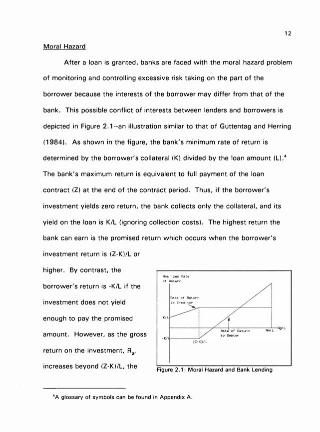
After a loan is granted, banks are faced with the moral hazard problem

of monitoring and controlling excessive risk taking on the part of the

borrower because the interests of the borrower may differ from that of the

bank. This possible conflict of interests between lenders and borrowers is

depicted in Figure 2. 1--an illustration similar to that of Guttentag and Herring

(1984). As shown in the figure, the bank's minimum rate of return is

determined by the borrower's collateral (K) divided by the loan amount (L).4

The bank's maximum return is equivalent to full payment of the loan

contract (Z) at the end of the contract period. Thus, if the borrower's

investment yields zero return, the bank collects only the collateral, and its

yield on the loan is K/L (ignoring collection costs). The highest return the

bank can earn is the promised return which occurs when the borrower's

investment return is (Z-K)/L or

higher. By contrast, the

borrower's return is -K/L if the

investment does not yield

enough to pay the promised

amount. However, as the gross

return on the investment, Rg,

increases beyond (Z-K)/L, the

Ree 1 1 zed R8te

of l=let�rn

Rate or RatlTn

to Cred 1 tor

"�---------?L-----�

cz- ()tL

Figure 2.1: Moral Hazard and Bank Lending

4A glossary of symbols can be found in Appendix A.

13

rate of return to the borrower rises and is maximized at Rm/L.

The riskiness of the loan affects the borrower and lender differently.

For example, the interests of the bank and the borrower may conflict if the

borrower prefers investments that are associated with the possibility of

relatively high returns and high risk. As shown in Figure 2.1, the borrower

accrues all returns in excess of the loan repayment, but the borrower's loss

is the same no matter how far below the default point the investment

returns fall. The bank, on the other hand, is indifferent to the amount of

profits the investor earns above the default point, but is interested in the

extent of loss if the investment return is less than the default rate.

The possibility of moral hazard is likely to be higher in a firm whose

business is failing. Such a firm has an incentive to take on higher risk

projects because of the hope that the commensurately higher expected

payoff will provide the added revenue needed for the firm to survive. If the

firm's risk-taking is successful, the firm will survive and its loan will be paid

in full; but if it is not successful, the firm will go bankrupt and the bank loan

will go into default.

Because of moral hazard, loan contracts generally contain restrictions

and protective covenants in an attempt to ensure full loan repayment.

Moreover, banks monitor loans by occasionally requesting financial

information from borrowers and by reconsidering a firm's financial status. 5

6These surveillance and monitoring activities of banks are called agency costs where banks are acting as an agent for their depositors' funds.

14

The Role of Banks in Commercial Lending

A market characterized by information asymmetries complicates the

loan pricing process because of the difficulties inherent in determining risk

with limited information. The role banks fill in commercial lending, however,

emerges from the need to overcome the problem of asymmetric information

in the credit market. 6 Campbell and Kracaw ( 1980) suggest that " ... in a

perfect market environment, intermediaries could perform no unique financial

service that investors would be unable to reproduce as easily. "7 However,

under information asymmetries, some profitable investment opportunities are

essentially nonmarketable but the information gathering and monitoring

expertise of banks enables them to find productive investment opportunities

among nonmarketable assets (Murton, 1989).

Most theories of commercial lending emphasize the abilities of banks

to evaluate and monitor loans.8 These theories can be further divided into

6See, for example, Boyd and Prescott (1986), Campbell and Kracaw (1980), Chan (1983), Diamond (1984), Fama (1985), Kane and Malkiel (1965), Leland and Pyle (1977), and Seward (1990).

7 As an alternative hypothesis to the proposal. that financial intermediaries exist to resolve information asymmetries, Campbell and Kracaw (1980) suggest that financial intermediaries are portfolio managers who would earn a competitive management fee in an unregulated

market. Under this alternative hypothesis, the U.S. banking system is a product of the regulatory environment. Therefore, problems surrounding information asymmetries are not critical in explaining financial intermediaries.

81n a review of banking models, Santomero ( 1 984) found that explanations for the existence of financial institutions are approached from three points of view: 1) their role as asset transformers through diversification potential and asset evaluation, 2) the nature of the liabilities they issue and their central function in a monetary economy, and 3) their two-sided nature (assets and liabilities). Because this paper is concerned with the asset side of banking, only theories explaining commercial lending are reviewed.

15

two categories: theories that explain the role of commercial banks as either

efficient or confidential evaluators and monitors of commercial loans. Both

of these explanations involve resolving information asymmetries.

Efficiently Evaluating and Monitoring Commercial Loans

Banks can efficiently evaluate and monitor loans because they can

diversify and access information that is not available to other capital market

participants.9 These two concepts are treated in turn.

Diamond (1984) developed a model in which diversification in the loan

portfolio is key to a bank's net cost advantage relative to direct lending and

borrowing. The model involves an ex-post information asymmetry between

potential lenders and a risk-neutral entrepreneur who desires to raise capital

for a risky project. Although the debt contract with which the entrepreneur

raises funds involves costs, it is possible for lenders contracting directly with

the entrepreneur to assume these costs by spending resources monitoring

the results of the investment that the entrepreneur observes.

If many lenders exits, the cost of monitoring may be large or a free

rider problem may exist where no security holder monitors because his or

her share of the benefit is too small. The free-rider problem is solved when

a bank monitors on behalf of those who provide the funds (depositors).

When participants are risk neutral, Diamond shows that diversification

increases the probability that the bank possesses sufficient loan proceeds to

9Chan (1983) has shown that financial intermediaries' role as informed agents leads investors to a higher welfare state.

repay a fixed debt claim to depositors. When a bank's number of loans

approaches infinity, the probability that the bank possesses sufficient loan

proceeds goes to one and the possibility of incurring necessary bankruptcy

costs goes to zero. Thus, banks efficiently monitor loans because of their

ability to diversify.

16

The second way banks efficiently evaluate and monitor loans when

asymmetric information exists is through their access to information not

available to others. According to Lummer and McConnell (1989), banks gain

access to this information by one of two methods: investment in

information-gathering technology or access to private information through

customer relationships.

Information-gathering technology in which banks invest include such

items as computers and software packages, data bases, and human capital.

Two widely used data sources that aid banks in their identification of risk

and price are Robert Morris Associates (financial ratio summaries for more

than 95,000 financial statements) and Loan Pricing Corporation (pricing

matrix created from over 6,000 commercial loans). Some banks also

maintain extensive databases of their own customer's loan characteristics

which loan officers can access to aid in their analysis. In addition, Altman

(1985) notes that many large banks run extensive simulations of repayment

and other measures of firm performance under alternative interest rates,

general economic, inflation, and key variable assumptions in their financial

17

analysis of potential borrowers.

Although current theory does not incorporate much about the

information technology banks use, the literature has focused on the ability of

banks to access private information through customer relationships.

Theories generally suggest that banks gather information through a

customer's deposit or loan patterns, and the private information they

possess about their customers increases over time. In each of these

theories, it is apparent that the marginar costs of monitoring are lower for

banks than for other financial intermediaries because of the structure of the

customer relationship.

In their seminal article on the information advantages gained through

customer relationships, Kane and Malkiel ( 1965) argue that when a bank and

customer develop a relationship through loans or deposits, the bank is able

to discern the quality of the customer.10 Moreover, the customer quality

becomes apparent to the bank because the bank's ability to forecast the

firm's future behavior is largely a function of the length of the relationship.

Black (1975) and Fama (1985) emphasize only the deposit relationship

between a bank and its customers to explain why banks monitor loans at a

lower cost than that of other financial intermediaries. According to this

scenario, the historical relationship of a borrower as a depositor provides the

10Hodgman (1961 b) is credited with first noting the importance of the bank-customer relationship. In particular, he asserted that "Anyone who troubles to inquire of commercial bankers will discover that the deposit relationship of a loan customer is a primary consideration in determining the cost and availability of bank credit to that customer."

18

bank with information that allows it to identify the risks of granting a loan to

a particular firm and enables the bank to monitor the loan at lower costs

than other lenders.1 1 Fama provides two facts to support this contention:

banks usually require borrowers to maintain deposits at its bank, 12 and

banks are the dominant suppliers of short-term inside debt.

More recently, Sharpe ( 1990) developed a dynamic theory of

"customer relationships" in bank loan markets in which long-term bank-

borrower relationships arise endogenously because of the asymmetric

evolution of information. According to this model, all banks begin with the

same amount of information when a new firm seeks a loan because no one

has information about the expected quality of the firm. The bank that loans

money to the firm, however, learns more about that firm's characteristics

than do other banks through the monitoring process. Consequently, as time

goes by, the bank that loans money to a particular firm is in an increasingly

better position than "outside" banks to evaluate the firm's future

performance.

Confidentially Evaluating and Monitoring Loans

In addition to efficiently evaluating and monitoring loans, banks

"Sanford Rose, an observer of the banking industry, wrote in the June 22, 1992 issue of the American Banker that small commercial borrowers transact between 50 and 300 credits and debits monthly, which enables a lending officer to easily understand the patterns of their commercial activity. He notes that checking account surveillance is much more difficult for large borrowers, particularly if they operate in several different regions or employ more than one bank.

12This requirement has been relaxed over the years, particularly for a bank's largest customers.

19

provide an additional service through the confidential manner in which they

treat the information they gather. Confidentiality is important for two

reasons: some borrowers desire to withhold information from their

competitors and some want banks to "signal" their firm's worth through the

loan approval process.

When firms acquire funds through public debt, they are required to

provide information that some firms prefer to keep confidential.13

Campbell ( 1979) posits that managers can preserve the monopoly profits for

the current owners of their firm by using a financing source that will monitor

its activities and yet keep the information confidential--banks fill this role.

On the other hand, some firms may use banks as a funding source

because banks signal to other capital market participants that the firm's

project is of high value. This value, which is directly related to the

asymmetric information problem, is explained in a theory developed by

Leland and Pyle ( 1977). They reason that when firms try to sell information

about their project directly to investors, concerns arise about the credibility

of the information and adverse selection. Because it is difficult or impossible

for some observers to determine whether the information is accurate, the

price of the information will reflect its average quality and thus market

13Some small firms, however, may be prohibited from obtaining debt in the capital markets because it is costly to provide the information required. Consequently, small firms might use banks to borrow funds because the bank pays the cost of information gathering. In fact, Blackwell and Kidwell ( 1 988) found that minimizing overall costs is the motive behind some firms decision to use private markets rather than issue public securities.

20

inefficiency will result--investments will not be priced properly and resources

might not be allocated properly.

The problems related to the transfer of information can be overcome

by banks that gather information and buy and hold assets on the basis of

their specialized information. Banks signal high value projects when they

loan funds for a project because they back their opinions with investments

of their own funds. 14

Essentially, the intermediary causes a sorting of classes of risk. The

entrepreneurs with projects that possess favorable risk characteristics wish

to be identified so they deal with an "informationally-efficient" intermediary

rather than with uninformed investors who would offer a price equivalent to

the average level of risk. According to Leland and Pyle, the best risks are

"peeled off," and thus the average risk becomes less valuable and induces

the owners of the next best risks to deal with the intermediaries. This

process continues until sellers of all types of risk sell to the intermediary

except perhaps those firms with the worst projects. 15

14Campbell and Kracaw ( 1 980) take this explanation a step further and demonstrate that initial wealth endowments resolve the moral hazard problem because they function as a guarantee of the reliability of the information when they possess a stake in the market large enough to override any incentive to misrepresent the information. This result leads to the conclusion that initial wealth endowments act as a barrier to entry in the market for information and as a general constraint on reliability.

16Leland and Pyle also propose that an entrepreneur's willingness to invest in his/her project serves as a signal of the project's quality. They posit that the value of the firm increases as the proportion of the firm owned by the entrepreneur increases. The logic behind this assertion

is clear: if an entrepreneur believes a project is associated with a high probability of success, then the entrepreneur will desire to own as much of the project as possible in order to accrue

(continued ... )

21

Fama (1985) reaches a similar conclusion when he considers what is

special about bank loans that causes borrowers to pay higher interest rates

than those on other securities of similar risk.16 He suggests that the

comparative advantage of banks as lenders (over other financial

intermediaries) involves their ability to minimize information costs because of

the positive signal they send when they renew a firm's short-term loans.17

The loan renewal process triggers a periodic evaluation of the borrower's

ability to repay its low-priority fixed payoff contract with the bank.18 By

renewing a firm's loan, banks send a positive signal to other agents with

higher-priority fixed payoff claims who now do not have to duplicate the

16( • • • continued) most of the profits. This explanation may be important to bankers as they seek to identify the quality of an entrepreneur's projects.

16ln Fama's model of banking, he considers only loans on the asset side and demand deposits and certificates of deposit (COs) on the liability side of the bank's balance sheet. Demand deposits are associated with a reserve requirement. According to the literature, the reserve tax is borne by depositors who accept a lower interest rate because of the special transaction services that they receive from the bank (such as redeemability for cash and checking accounts). Cds also carry a reserve requirement but provide no apparent transactions or liquidity services relative to commercial paper and bankers' acceptances--two securities whose yield and risk is similar to that of COs. In addition, the yield on COs and bankers' acceptances of the same maturity are almost identical and the difference between average yields on COs and commercial paper are trivial. Thus, Fama argues, that since COs must pay competitive interest rates, the reserve tax on the COs is borne by bank borrowers. Hence, there must be something special about bank loans that makes some borrowers willing to pay higher interest rates than those on the other securities of equivalent risk.

17Fama also suggests that firms use banks to obtain funds instead of publicly traded debt because of contract costs--it is cheaper to give one agent (the bank) access to information within the firm than to produce the information associated with outside-debt financing.

'8Banks generally are last or close to last in the line of priority among an organization's contracts that promise fixed payoffs.

22

cost of obtaining information about the firm.19 Bank signals are credible,

according to Fama, because the bank backs its opinions with resources (in

terms of a loan) or by declining resources (if bad loans are made).

Summary

Due to information asymmetries, banks have developed an expertise in

efficiently gathering and monitoring information. This access to information

enables banks to find profitable investment projects that would otherwise be

unmarketable. Moreover, the confidential manner in which banks handle this

information and the signal they transmit by granting a loan, provides an

additional value to some borrowers who could obtain investment funds

through alternative and perhaps less costly sources (see Figure 2.2).

The information that banks obtain about loan applicants enables them

to resolve information asymmetries and price loans. The unanswered

question, however, is how banks determine loan prices and whether those

prices are related to risk or some other characteristic of the loan. The next

chapter presents three theories that provide greater insight into how banks

might price commercial loans.

'9James (1987) provides empirical support consistent with the uniqueness of banks and information-effect hypotheses. Specifically, James found that a statistically significant positive abnormal return accrues to stockholders of firms when they publicly announce bank credit agreements. Also, the announcement of publicly placed straight debt issues were associated with negative stock evaluations as suggested by the information-effect hypothesis (see, for example, Leland and Pyle, 1977). Lummer and McConnell (1989) and Best and Zhang (1992) have also found empirical support that the bank lending process transmits information to the securities market about the quality of the borrower.

Two Main Reasons

Businesses Borrow

From Banks

� -------------.. Confidentiality

M-V/ Port Credit Ration 1 ng

No Entrance into

Customer Relationships

Figure 2.2: A Conceptual View of the Market for Commercial Loans

23

CHAPTER Ill

THEORIES ADDRESSING COMMERCIAL LOAN PRICING

The purpose of this chapter is to use the following three theories to

explain the factors that might influence the way banks price commercial

loans: 1) mean-variance analysis and portfolio theory, 2) credit rationing by

default risk, and 3) customer relationships. Although these theories were

not developed for the purpose of explaining loan pricing, each implies a

theoretical basis with which to test loan pricing practices. These theories

overlap in some respects, but each implies a unique view of loan pricing.

Mean-variance analysis and portfolio theory, which are reviewed first,

indicate that loans should be priced relative to the risk of the individual loan

as well as the loan's contribution to the variability of the bank's entire loan

portfolio. Rather than increase the contract interest rate on a loan to control

for risk, however, the theory of credit rationing indicates that some loans are

denied because, beyond a particular interest rate, the additional risk of a loan

outweighs the possible increase in revenues from the higher interest rate.

Finally, customer-relationship theories suggest two divergent views of

pricing. The earliest customer relationships theories propose that loans

should be priced by the long-term profits that the customer is expected to

contribute to the bank. Consequently, loan pricing takes into account the

24

25

return expected from such factors as the volume and variability of a

customer's deposit. One view holds that longer customer relationships are

equated with lower priced loans. An opposing theory argues that long-

standing customers are priced relatively higher than others because these

customers are "informationally captured"--unable to convince other lenders

of their superior repayment record.

Mean-Variance and Portfolio Theory in Loan Pricing

Financial theory indicates that assets are priced relative to risk, and

portfolios are diversified such that the expected return is maximized for a

particular variance or the variance is minimized for a particular expected

return. In terms of loan pricing, this theory indicates that loans should be

priced relative to their individual risk as well as their contribution toward the

total variability of the loan portfolio.

Mean-Variance Analysis

Mean-variance analysis indicates that the return and risk of an asset is

represented by the mean and variance of its expected return (Markowitz,

1952) .1 The mean measures the most likely outcome of a set of events

1The mean and variance alone can be used to represent an asset only when the expected returns of the asset are normally distributed or if the investor possesses a quadratic utility function which describes risk-averse behavior. Nevertheless, the distribution of expected returns to the bank on a loan contract is skewed rather than normal because returns are limited by the amount of the loan contract. Some empirical evidence exists, however, that banks possess quadratic utility functions with regard to the rate of return on assets. Also, other utility functions are locally approximated by quadratic utility. (For a further explanation of the relevance of quadratic utility in mean-variance analysis see Elton and Gruber, 1 987 . ) In

(continued ... )

26

and, in the case of loans, is defined as

N

(3.1) E(R)=}: d� i•1

where d; is the probability of a random event, R;, and N is the number of

possible events. 2 Risk is defined as the variance of possible outcomes.

Mathematically, the variance (VAR) is defined as the expectation of the

squared difference from the mean:

(3.2) VAR=E[(R;-E(R))2j.

Banks do not use equation (3.2) to measure a loan's risk because of

the difficulties in measuring expected return. Instead, banks use their

information gathering skills to determine the loan's risk rating (a measure

that reflects default risk or the probability that a lender will not repay the

loan) which is used to determine the contract interest rate.

The literature that considers loan pricing in terms of default risk

suggests that the relationship between default risk and price is similar to

that between the loan's expected return and the variance of the expected

return. Flannery (1985) and Sinkey (1989) represent the relationship

between default and the loan contract interest rate by first abstracting from

1 ( • • • continued) addition, Hester and Pierce (1975) note that banks are likely to be risk averse, either because their objective functions are convex in discounted future net income or because influential depositors and/or regulators encourage them to act as risk averters.

2A glossary of symbols can be found in Appendix A.

27

resource costs such as overhead. The loan contract rate, i ·, required

compensate the lender for the time value of money as reflected in the

nominal rate of interest, i, and the probability of default, d. This relationship

can be expressed as:3

(3.3) ;·= (1 +i) -1 (1-d)

As shown in Figure 3.1, this relationship is consistent with mean-variance

analysis: loans that are perceived to carry higher risk are priced relatively

higher than low risk

loans. Moreover, the

relationship is linear in

the relevant range.4

Portfolio Theory

In addition to

pricing individual loans, PI""'CCCC&DIII't.y O't" O.'f"aUI't

portfolio theory Figure 3.1: Contract Interest Rate vs. Default Risk

(Markowitz, 1952; Tobin, 1958) suggests that investors choose their total

loan portfolio to maximize expected return for a given variance or to

3 Jaffee and Modigliani ( 1969) show that this relationship is the first-order optimization of a bank's loan offer curve.

4Historical data indicate that the spread between the loan rate and opportunity rate at which banks can obtain funds or invest funds is typically small. The implication is that banks will generally assume modest default risk because their interest rate spread restricts them to a small margin of error. If the cost of funds equals 5 percent, for example, and a bank prices

a loan 50 basis points above cost, the price is implicitly assuming that risk is 0.0048 percent probability of default.

28

minimize the variance for a given expected return--an efficient portfolio.5

The expected return for a portfolio of assets is simply the weighted

average of the expected returns for the individual loans in the portfolio.

Calculating the variance of the portfolio's returns is not as straightforward.

It is the squared weighted average of the individual variances plus two times

the weighted covariances between all the loans in the portfolio:

N N N

(3.4) VARP = L x�VA� + 2L L x�povii. j:1 i•1 j•1

where VARP is the variance of the loan portfolio, VAR1 is the variance of

loan i, COV;i is the covariance between the returns on loans i and j, and x is

the fraction of the portfolio represented by the loan. The formula for the

portfolio variance shows that, in addition to the variance of individual loans,

the covariances between pairs of individual loans is incorporated in the

variance of the total loan portfolio. The variance of a portfolio with a large

number of loans can be stated as the summation of its weighted

covariances:

N N

(3.5) VARP =2L L x�pOV;i i=1 j=1

Thus, the contribution of a loan's riskiness to the total portfolio is

determined by its average covariance with all the other assets in the

portfolio rather than simply the individual loan's variance.

6Hart and Jaffee (1974) have shown that the separation theorem holds for depository financial intermediaries. They also found that the efficient frontier space is linear.

29

In general, portfolio theory indicates that if a bank holds many

different types of loans in its portfolio, it can achieve a lower variability of

actual loan losses for the same rate of return. In other words, maximization

of return at a certain risk level implies a diversified portfolio.6 The lower the

correlation of return between loans, the lower will be the risk of the entire

portfolio. Thus, portfolio theory implies that banks are not only concerned

with the risk of a single loan, but with the loan's contribution to the

variation of the total loan portfolio. Consequently, loans should also be

priced relative to the bank's loan portfolio.7

Summary

Mean-variance analysis and portfolio theory imply that commercial

loans should be priced relative to their individual risk as well as their

contribution to the variation in the bank's total loan portfolio. According to

this theory, price serves as the rationing mechanism. That is, when the

demand for loans exceeds supply, banks ration some potential customers

out of the market by raising the contract interest rate.

8McManus (1992) provides empirical evidence that diversification can be a powerful force in reducing the riskiness of bank loan portfolios. ·

7 Applications of portfolio theory to bank loan portfolios have been limited because of the difficulty in computing the expected return and variance on loans. Appendix B considers in more detail the unique methods that several authors have proposed to apply portfolio theory

in banking. In general, these articles propose that banks measure risk concentrations within their portfolio so that the pricing of new loans can account for the impact of the new loan on the variability of the portfolio's total return.

30

Credit Rationing by Default Risk

Instead of pricing loans strictly based on risk, credit rationing theories

posit that banks control risk by denying credit to the riskiest borrowers. In

other words, banks price loans up to a maximum interest rate, which is

associated with a particular level of default risk, and beyond that rate banks

do not loan funds regardless of the interest rate offered by the potential

borrower.8 Credit is rationed with asymmetric information because adverse

selection and moral hazard increase the possibility that higher contract

interest rates will be associated with losses that outweigh the expected

return from the increase in interest rates. Therefore, credit rationing theories

imply a nonmonotonic relationship between the expected return on the loan

and the contract interest rate.

Early Theories of Credit Rationing

The earliest theories of credit rationing grew out of the availability

doctrine9 which sought to explain the efficacy of monetary policy by

8More precisely, credit rationing has been defined as an excess demand for commercial loans at the loan rate quoted by the banks (Jaffee and Modigliani, 1 969) because quoted loan rates are below the Walrasian market-clearing level (Jaffee and Stiglitz, 1990).

9The availability doctrine became prominent at the end of World War II when empirical evidence suggested that the accepted theory of monetary policy would not enable the Federal Reserve Board to effectively carry out its policies. At the time, it was believed that for monetary policy to be effective, real expenditure decisions needed to be interest elastic, and the central bank needed the ability to force changes in relevant interest rates. Empirical studies, however, found little interest elasticity, and the Treasury restrained the Federal Reserve's ability to influence interest rates on government debt. Consequently, the availability doctrine developed as an alternative for the efficacy of monetary policy. Proponents of the doctrine argue that monetary policy is effective because financial institutions reduce the availability of funds rather than through changes in the cost of funds, which was thought to be the mechanism of change in the then prevalent view of monetary policy (Scott, 1957).

31

reductions banks made in the availability of their loanable funds. The first

models of credit rationing use various credit market imperfections to show

that it is rational for profit-maximizing banks to deny some requests for

credit rather than to raise interest rates when the demand for loans exceeds

supply (Freimer and Gordon, 1965; Hodgman, 1960; Jaffee, 1971; and

Jaffee and Modigliani, 1969; Miller, 1962). Hodgman and Jaffee and

Modigliani are summarized here because· they were the two most influential

of the early credit rationing models.

Hodgman's (1960) model suggests that rational profit-maximizing

banks use the riskiness of customer loans as the criterion to ration credit.10

He defines loan risk as the ratio of the expected value of the payoff from a

loan to the expected value of loss (payments below the agreed upon

contract). Furthermore, Hodgman assumes that banks require a loan risk

ratio above the equilibrium ratio that exists in a perfectly competitive market;

and he demonstrates that as the size of the loan increases, the risk ratio can

be kept above the equilibrium figure by increasing the interest rate. Beyond

a certain loan size, however, increasing the interest rate will not prevent a

decrease in the risk ratio (at this point the supply curve becomes backward

bending). Thus, the bank will not grant a loan, but will ration credit to a

prospective borrower who wishes to borrow an amount larger than this

100ne year later, however, in response to a critique of his 1960 article, Hodgman (1961 a) said he now thought bank credit rationing was not caused by risk considerations but by the

effort of bankers to maximize long-term profits through favored loan treatment of profitable depositors-borrowers.

32

maximum, regardless of the interest rate the borrower offers.

Jaffee and Modigliani (1969) show that the principle of increasing

default risk with increasing loan size and the narrow spread of loan rates

over cost (caused by ceiling interest rates) creates a situation where it is

rational for profit-maximizing banks to ration credit. They base the reason

for credit rationing on the fact that banks classify borrowers into a small

number of groups.11 Within each class, the bank charges a uniform rate

even though the firms within a group may be diverse with respect to risk

and the amount of their loan demand. The group loan rate is selected to

maximize bank profits over the entire group. Some firms, however, are

rationed because they possess above-average demand or above-average risk.

Consequently, rationing may occur in every risk class.

Early models of credit rationing show that it is rational for profit-

maximizing banks to ration credit rather than to increase contract interest

rates when demand exceeds supply.12 In terms of loan pricing, these

11These groups are based on objective factors such as type of industry, asset size, and standard financial measures. Jaffee and Modigliani conclude that bankers can best exploit their market power by classifying customers into a small number of classes because of the ceiling price caused by considerations of good will, social mores, and legal restrictions. The incentive to adopt a segmented classification exists because banks desire to maintain rates as close as possible to the collusive optimum, but cannot openly collude. The use of a small number of risk classes, based on readily verifiable objective criteria, appears to be an efficient way to optimally price loans without competitively underbidding other banks. This classification structure is also facilitated by tying rates to a prime rate that is set through price leadership.

12Empirical tests which support the view of credit rationing on an aggregate banking level include Fair and Jaffee (1970), Jaffee (1968), Jaffee and Modigliani (1969), and Silber and Polakoff (1970). This research generally focuses on the speed with which commercial loan rates adjust to changes in open market rates. A finding of "sticky" rates supports credit rationing because it implies that the credit markets do not respond to demand by changing

(continued ... )

33

models predict that banks will price loans relative to risk but will choose a

cut-off contract interest rate that is associated with maximizing their profits.

However, the early models did not explain the underlying cause of credit

rationing.

Credit Rationing Based on Imperfect Information

The most recent theories of credit rationing use imperfect information

to explain why rational profit-maximizing banks ration credit.13 This section

reviews the credit rationing model developed by Stiglitz and Weiss (1981)

and further explained by Jaffee and Stiglitz (1990) because it provides

insight into loan pricing by explaining why the relationship between the

loan's expected return and contract interest rate is parabolic. In particular,

their model implies that beyond a certain point, interest rates do not

compensate sufficiently for risk because"the negative adverse selection and

incentive effects that accompany relatively high rates may outweigh the

increase in return from those higher rates as shown in Figure 3.2.14 Thus,

12( • • • continued) price. Slovin and Sushka (1983), however, find that commercial loan rates are not sticky during the period 1953 to 1980. Also, Berger and Udell (1989) provide empirical evidence that credit rationing is not an important macroeconomic phenomenon in a test based on over 1 ,000,000 commercial loans.

13Akerlof (1970) and Rothschild and Stiglitz (1971) first suggested that imperfect information played a role in loan markets while Jaffee and Russell (1976) were first to apply the concept in a model of credit rationing.

14Similarly, Guttentag and Herring (1984) propose an asymmetric information model, but they include the borrower's capital position, default risk, and a probability that nature will draw

from a disastrous distribution. Their model indicates that lenders maximize expected return when the expected value of the increase in the· contract rate when the borrower does not default equals the expected loss caused by the induced increase in the probability of default.

34

equilibrium in the credit market may be characterized by credit rationing or

excess demand.

To show that credit rationing can exist and that the relationship

between the bank's expected return and contract interest rate is parabolic, it

must be shown that the expected

return a bank receives does not

increase monotonically with the

interest rate charged.

Nonmonotonicity can be shown by

either adverse selection effects or

adverse incentive effects. These

two concepts are explained in turn.

As noted in the previous

Bcpected Ret.1.rn

on tN L..oan

I ntereet Alrte

�--------�,�.--------==�

Figure 3.2: Relationship Between Expected Return and Risk.

chapter, adverse selection occurs because low-risk borrowers may drop out

of the market as rates rise and because banks are unable to identify with

certainty those borrowers who will repay their loan in full. Stiglitz and

Weiss argue that interest rates may act as a screening device15 in this

environment because individuals willing to pay relatively high interest rates

may, on average, be worse risks: they are willing to pay high rates because

they do not anticipate repaying the loan.

'6Guttentag and Herring (19841. Milde and Riley (19881. and Schreft and Villamil (19921

also argue that contract interest rates on loans act as a signalling device of the borrower's characteristics when lenders possess imperfect information.

35

An example illustrates how the mix of loan applicants changes

adversely when interest rates increase. In this example, the bank identifies a

group of projects and for each project, 9, there exists a distribution of gross

returns, Rg.16 (Appendix A contains a glossary of symbols.) Moreover,

assuming that the bank can distinguish projects with different mean returns

but cannot identify the riskiness of a project, the F(Rg,(J) is the bank's

subjective perception of the project's distribution of returns and f(Rg,(J) is the

associated density function. This example also assumes that increases in (J

correspond to greater risk. Finally, L is the amount a firm borrows at

contract interest rate i", and the firm defaults if the return plus collateral, K,

is insufficient to repay its loan: K + Rg � L(1 + i").

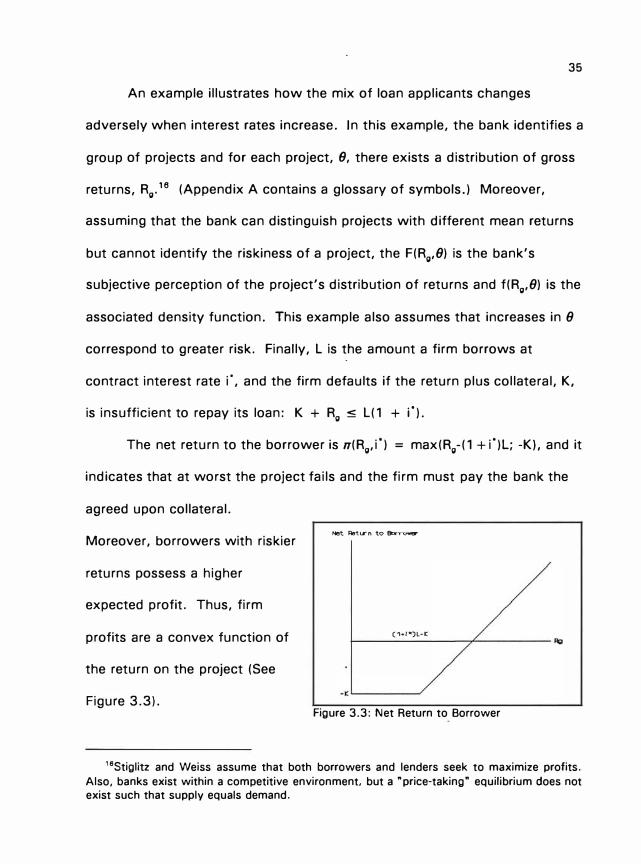
The net return to the borrower is rr(Rg,i") = max(Rg-(1 +i")L; -K), and it

indicates that at worst the project fails and the firm must pay the bank the

agreed upon collateral.

Moreover, borrowers with riskier Net Ret I¥ n to Borrower

returns possess a higher

expected profit. Thus, firm

profits are a convex function of (1-+l�t)L-t::::

the return on the project (See

Figure 3.3). -<'-------'

Figure 3.3: Net Return to Borrower

16Stiglitz and Weiss assume that both borrowers and lenders seek to maximize profits. Also, banks exist within a competitive environment, but a "price-taking" equilibrium does not exist such that supply equals demand.

The return to the bank is

written as p(Rg,i') = min(Rg + K;

L(1 +i")) which indicates that the

bank will collect either the

maximum that the borrower can

repay if the project fails or the

agreed upon interest and

36

Alttl.rn to BD'*=:

(hl"')l-t:

Figure 3.4: Return on Loans to Banks

principal if the project is successful. As shown in Figure 3.4, the return to

the bank is a concave function of the return on the project. Thus, expected

return decreases as risk increases because the probability of default

increases.

Given the convex nature of the return of the project to firm profits, a

critical value (risk) iJ exists for a given interest rate i" such that a firm will

borrow if and only if 0 > IJ. As interest rates rise, the critical value of iJ

increases, which means that investors with less risky projects are unable to

make a profit. Thus, they drop out of the market and the mix of applicants

worsens. At the same time, the concavity of the bank's return indicates

that the expected returns to the bank are smaller with higher loans.

Therefore, although an increase in the interest rate increases the bank's

return, an adverse-selection effect may be acting in the opposite direction.

Another example clarifies the possibility that the adverse effect

outweighs the direct effect of an increase in interest rates. Assume only

two groups of borrowers exist:

a safe group that borrows only

when the interest rate is below i-

1 and a risky group that borrows

only when the interest rate is

below i-2 where i-1 < i-2.

El<pect.ed Ret...,... n

on 'tha Loan

Both Typee

AI:!Piy for

Loa,...

37

1-1 1-2 Quoted Loan Rate

When interest rates are slightly

above i-1, the mix of applicants

Figure 3.5: Mix of Applicants Worsens with High

Rates

changes dramatically as shown in Figure 3.5 because all of the low-risk

applicants withdraw.

The second way changes in interest rates might adversely affect bank

profits is through their impact on the borrower's behavior or moral hazard.

Raising the interest rate associated with a project obviously decreases the

returns on that project to the investor. However, higher interest rates may

also induce firms to take on projects with lower probabilities of success but

higher payoffs when successful.

To show that interest rates act as an incentive mechanism, it is

assumed that firms may choose alternative projects. The two projects

considered here are denoted by superscripts "j" and "k." First, Stiglitz and

Weiss establish that if, at a given contract interest rate i'', a risk-neutral firm

is indifferent between two projects, an increase in the interest rate causes

the firm to prefer the project with the higher probability of bankruptcy. The

increase in i" lowers the

expected return to the borrower

from the relatively safe project

more than it lowers the expected

return from the project that

Elcpect.ed Reurn

to the Borrower

Project J

38

Proj.a J

carries a higher risk. This is �------------,�-

--------����-�L�n

shown in Figure 3.6 where the Figure 3.6: Rates as an Incentive Mechanism

borrower chooses risky project j when i" increases beyond i"". As a result,

raising the interest rate above i"" might increase the riskiness of loans

enough to lower the expected return to the bank.

In summary, credit rationing predicts that loans will be priced such

that the expected return on the loan reaches a maximum at a particular rate

and beyond that rate declines relative to the contract interest rate.

Consequently, i" serves as a signal of loan quality.

Collateral and Credit Rationing

Collateral requirements provide another mechanism for banks to price

loans. Stiglitz and Weiss (1981) propose that increasing collateral

requirements or the fraction of the project financed by equity is not a good

means of allocating credit when an excess demand for funds exists and

when the contract interest rate is fixed. Under these circumstances,

increasing collateral requirements beyond some point may also decrease the

bank's returns by either decreasing the average degree of risk aversion of

39

the pool of borrowers or encouraging borrowers to undertake riskier

projects.17

In contrast, some argue that credit rationing is avoided when a bank

can set collateral requirements and interest rates simultaneously .18 Sarro

( 1976), for example, argues that collateral functions as an incentive for

borrowers to repay their loans; and in the case of default, provides some

return to the bank. As such, he argues that the unwillingness of banks to

lend in the Jaffee and Modigliani-type theories do not reflect credit rationing

but reflects (p. 448) " ... the upward slope of the loan supply curve graphed

versus the appropriate price that includes a consideration of collateral."

Jaffee and Stiglitz ( 1990), however, argue that the collection of collateral

may reduce but generally does not eliminate the risk of default because

collateral may be uncertain and transactions costs may be associated with

its liquidation.

17This conclusion is contrary to that of Leland and Pyle (1977) who argue that an investor's proportion of equity in a project provides a positive signal of its expected success. However, in a study written after the one noted above, Stiglitz and Weiss (1986) show that collateral decreases risk when collateral and interest rates are set simultaneously.

18Similarly, Guttentag and Herring (1984) show that an increase in a borrower's capital (asset value) position limits the possibility of moral hazard. This occurs because the optimal riskiness of an investment project to a borrower increases as the contract rate rises; but the optimal degree of riskiness declines as a borrower's capital position increases. In fact, they show that moral hazard disappears when the capital position of the borrower equals the total payment from the borrower at the end of the contract period because the borrower cannot increase his or her expected return by taking on riskier projects. With no capital position, however, the borrower can obtain the maximum benefit from increasing the riskiness of the investment. Consequently, the lender is most vulnerable to moral hazard when capital is minimal.

40

Summary

Theories of credit rationing indicate that rational profit-maximizing

banks may decline some loans rather than let price act as the rationing

device. In addition, recent theories conflict on whether increasing collateral

exacerbates or mitigates moral hazard. The implication of these theories for

loan pricing is that contract loan rates act as a signal of loan quality; and

because of adverse selection and incentive effects, the relationship between

a loan's expected return and contract interest rate is curvilinear.

Loan Pricing and Customer Relationships

Customer relationship theories propose that customers who contribute

more to the bank's long-term profitability are given loans with lower rates.

These theories, however, disagree on the effect that the length of the

relationship plays in pricing.

Importance of Customers in Providing Deposits

The earliest theories of customer relationships developed in response

to credit rationing by default risk and centered on the importance of

customers in providing deposits. These theories argue that during times of

expanding credit demand, customers who are not preferred might be denied

loans so that funds will be available for the preferred customers who desire

41

more credit. 19

Hodgman (1961) was first to emphasize the importance of the

customer relationship. He argued that deposits are important to banks

because they are a principal and profitable source of the bank's ability to

lend and invest. The size of a bank's portfolio of earning assets relative to

equity capital is a function of the amount of its deposits, and the deposits

are a function of the services provided to deposit customers, including loan

accommodations. 2° Consequently, when deposit customers provide the

bank with net income in excess of the activity costs of their account, they

are granted loans with lower rates than other customers, particularly

nondepositors. In addition, deposits are particularly dear to banks during

times of strong loan demand.

Kane and Malkiel (1965) also argue that deposits play a role in the

importance of a customer relationship. They show that increases in the

volatility of individual or aggregate deposit balances unambiguously worsens

a bank's portfolio because it, ceteris paribus, increases aggregate risk

19After completing a survey of bankers, Hodgman (1963) concluded that in contrast to credit rationing by default risk (p. 149): "In the bank-customer relationship, however, we have another explanation for credit rationing which does not depend upon risk or uncertainty and which can be related directly to observed bank practice. At the heart of the customer relationship is the mutual dependence on loans and deposits. •

20Hence, bankers will maximize their lending capacity by giving priority to the loan requests of their largest depositors.

42

exposure and thus reduces both short- and long-run profits.21 In addition,

deposit variability decreases expected pr.ofits if the costs of asset acquisition

and sale are considered or if it is assumed that deposit flows and asset

yields are inversely related. As a result, a class of customers, c·, exist

whose past behavior contributes an important and favorable role in

determining the bank's expected profits and aggregate risk exposure. Thus,

loan denials to c· requests may cause customer alienation and loss of

important deposit relationships.

These deposit-relationship theories were developed within a regulatory

environment that was more restrictive than that which exists today and a

less developed market for corporate bond issues. Despite the substantial

changes in the banking environment over the last decade, deposits remain

an important low-cost source of funds for banks. Hence, loan pricing

practices could still be expected to reflect the importance of deposits.

Other Important Borrower Characteristics

Kane and Malkiel (1965) argue that, in addition to deposits, the c·

customers are described by a vector whose elements are indices of the

account's current size, future growth prospects, length of its attachment to

the bank, the apparent cohesion of that attachment, and the cyclical pattern

21Harrison and Meyer (1975) found that increases in deposit variability reduces bank profits because it forces banks to increase their holdings of liquid assets tat the cost of being more fully loaned.

43

of the customer's loan needs. 22 Obviously, large accounts are preferred to

small ones, growing accounts are more valuable than declining ones, stable

deposits are preferred to volatile deposits, old accounts are preferred to new

accounts,23 and cohesive accounts are preferred to footloose ones.24 The

characteristics noted here affect both the short-run and long-run bank

profits. Consequently, one would expect banks to charge lower contract

loan rates to customers with favorable characteristics. In the short run, c·

customers would be associated with a smaller return on loans than non-C'

borrowers. In addition to the above advantages, the marginal cost to

investigate the new loan requests of c· borrowers are much lower than that

for new customers.

Given the importance of c· customers, the relevant marginal

calculation of granting a loan is not whether the additional profit from

making the loan outweighs the increased risk. Rather, a utility maximizing

bank may agree to grant a c· request even though, compared with its

prerequisite optimum, it is associated with a decrease in utility because not

granting the loan also decreases utility. This implies that bankers must

22Some C" borrowers are important to lenders because their borrowing needs are greatest at times other than peak credit demands. Kane and Malkiel suggest two ways to measure this characteristic: the customer's expected mean indebtedness over typical cycles of loan demand and the coefficient of correlation between the customer's outstanding loans and aggregate excess demand for loans at the bank.

23As a banker's experience with an account increases, he or she should be better able to predict its behavior.

24The durability of the past customer-bank relationship should reduce the bank's estimate of outcomes around the mean. In other words, its variance.

44

consider the benefit and costs of an entire customer relationship in order to

price loans. 25

Customer Relationships with Asymmetric Information

Both the theory of Hodgman and Kane and Malkiel assume that

bankers possess full and certain information needed about borrowers. In

contrast, Sharpe ( 1990), assumes an asymmetric environment. 26 His

dynamic theory of customer-relationships suggests that long-term bank-

borrower relationships arise endogenously because of the asymmetric

evolution of information, and these relationships create the potential for ex

post or temporary monopoly power even though banks are ex ante

competitive. 27

According to Sharpe's theory, high quality firms continue to transact

business with a particular bank, not because they are treated particularly

well, but because they are "informationally captured." This situation occurs

because in the process of lending, a bank learns more than others about_ its

customers. Thus, the bank that loans to the high quality firm offers it a

26From the bank's view, the discounted income stream associated with the services to depositors equals a lump-sum benefit that is tied to customer loans. This benefit may outweigh the benefits of the higher contract interest rates obtained from nondepositor loans.

261n this theory, the key informational asymmetry that affects pricing is that which occurs between banks rather than between banks and borrowers. According to Sharpe (1990, p. 431:

"Rather than moral hazard, it is the potential for taking advantage of captive customers, by altering the terms of trade, that gives rise to a reputation equilibrium where competitors earn rents over time."

27 Jaffee and Stiglitz ( 19901 also argue that the information costs of determining default create a tendency toward natural monopoly in the supply of credit to a particular person, firm, or industry.

45

lower rate, when compared with other banks (although the lower rate still

allows the bank to accrue rents). Competing banks do not offer lower rates

than the bank which currently serves the customer because it is difficult for

the borrowing firm to convey information to other banks about its superior

performance.28 Moreover, adverse selection makes it difficult for a bank to

attract another bank's good customers without drawing the bad customers

as well.

Although banks are expected to earn no profit over the life of an

average customer relationship, an inefficient allocation of capital occurs

because the market does not force banks to offer better rates to their higher

quality customers than to their lower quality customers. Consequently,

banks can expect to earn economic profits on their better customers. These

rents are competed away, however, because competition forces banks to

grant lower interest rates on loans offered to new customers (when banks

possess the least information about the firms). As a result, lower quality

firms acquire a larger proportion of the bank's capital than in the standard

asymmetric information case. 29

28Sharpe's theory presents important information about the far-reaching economic impact of bank failures which is consistent with Bernanke's (1 983) explanation that the rise in the cost of credit from the collapse of financial institutions may have contributed to the depth of the Great Depression. Specifically, Sharpe implies that when a bank fails, its best customers are unlikely to find another bank that will lend to it as cheaply. In this case, it is possible that the additional interest burden placed on the firm will cause it to lower working capital investment which ultimately may lead to less production, employment, and even bankruptcy.

29Sharpe's theory suggests that the inefficiencies just noted can be reduced if banks develop reputations based on nonbinding promises. As future market participants learn that

(continued ... )

46

Empirical Test of Customer Relationships

The few empirical tests of customer relationships that were identified

provide support that these relationships play a role in pricing. Using a

sample of 3 large banks, Hester ( 1979) found that deposit balances and the

number of years the depositor had been with the bank favorably affected the

terms of the customer's loan. Also, Murphy (1969) found indirect support

that depositors receive some reduction in the price of loans vis-a-vis

nondeposits. In a more extensive study of 674 loans collected in 1972 from

62 banks, Hester ( 1979) found, ceteris paribus, borrowers with larger

demand deposit balances are charged lower contract interest rates on loans.

Also, previous borrowers from the bank received lower interest rates than

first-time borrowers. In general, he concludes that (p. 355)

... a bank determines loan amount in large part by evaluating the

nature of its relationship with a borrower. Once the decision to

lend and the loan amount are settled, a bank apparently looks

to collateral for protection and to a differential in the interest

rate to compensate itself for risk exposure.

Hester's results also provide some support for Sharpe's theory. In

particular, he found that borrowers who are considered "highly profitable

customers to the bank in the past" are charged new loan rates that are

relatively high when compared with all other customers.

29( ... continued)

the bank keeps its promises, wimplicit contractsw arise. These commitments are characterized

by prices that more closely approximate the optimal prices, and therefore lead to a more efficient allocation of capital.

47

Summary

The customer-relationship approach to pricing suggests that, in view

of a bank's total portfolio and long-term profits, some customer relationships

provide a greater net contribution to profits than others. Therefore, these

preferred customers are charged lower contract interest rates on loans than

other customers. Moreover, a bank might ration credit to other applicants

during times of rising credit demand in order to ensure available credit for its

preferred customers.

In an environment of asymmetric information, however, Sharpe

suggests that a bank's long-term customers become informationally

captured such that they cannot obtain a lower contract interest rate at

another bank. In this model, the asymmetric evolution of information

creates ex post monopoly powers for the bank; but the market for new

customers remains competitive. Thus, long-standing customers are charged

relatively higher contract interest rates compared with new customers.

Moreover, to the degree that banks lend to new customers at interest rates

that are initially low, these accounts are likely to generate losses.

Summary Comments and General Hypotheses

As reviewed in this chapter, portfolio theory as well as the theories of

customer relationships and credit rationing provide information about loan

pricing. Although these theories overlap to some degree, each suggests

48

unique predictors of the expected return on commercial loans which are

determined by pricing procedures (See Table 3.1 ). Mean-variance analysis

and portfolio theory indicate that risk is the most important predictor of

expected return. In contrast, credit rationing theories suggest that the loan

contract rate is the most important determinant of expected return, and the

relationship between these two variables is curvilinear. Although recent

theories agree that the relationship is caused by adverse selection and

incentive effects, they conflict on whether increased collateral requirements

reduces the negative adverse affects.

Finally, customer relationship theories suggest that a number of

customer characteristics affect loan pricing, but these theories propose

conflicting explanations of the length of customer attachment to the bank.

Some customer relationship theories indicate that better customers,

including those who have borrowed from the bank for a long period of time,

are more highly valued customers and thus are charged lower rates. In

contrast, Sharpe's theory of customer relationships posits that banks charge

relatively high rates to customers who have dealt with the bank for a longer

period and charge relatively low rates to new customers.

The general research question to be tested in this study is how banks

price commercial loans. The theories reviewed in this chapter imply several

hypotheses that provide information about the research question.

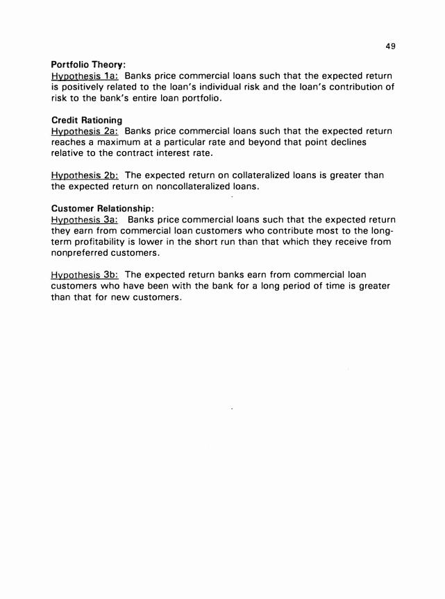
49

Portfolio Theory:

Hypothesis 1 a: Banks price commercial loans such that the expected return is positively related to the loan's individual risk and the loan's contribution of risk to the bank's entire loan portfolio.

Credit Rationing Hypothesis 2a: Banks price commercial loans such that the expected return reaches a maximum at a particular rate and beyond that point declines relative to the contract interest rate.

Hypothesis 2b: The expected return on collateralized loans is greater than the expected return on noncollateralized loans.

Customer Relationship:

Hypothesis 3a: Banks price commercial loans such that the expected return they earn from commercial loan customers who contribute most to the long­term profitability is lower in the short run than that which they receive from non preferred customers.

Hypothesis 3b: The expected return banks earn from commercial loan customers who have been with the bank for a long period of time is greater

than that for new customers.

50

Table 3.1: Summary of Theories Applied to Loan Pricing

JMQry Mean-Variance

Portfolio

Credit Rationing

Stiglitz and

Weiss (1981)

Guttentag and

Herring (1984)

Implied

Relationship

Figure 3.7

Figure 3.7

Figure 3.8

Figure 3.8

Customer Relationship

Hodgman (1961) Figure 3.9

Kane and Malkiel

(1965)

Sharpe (1990) Figure 3.10

Rationing

� Price

Price

Risk

Risk

Long-Run

Customer

Profit

Not

Applicable

Implied

Determination

� •Individual Risk

•Contribution to Portfolio Risk

•Interest Rates as Signal

•Collateral as Signal

•Collateral Solves Moral Hazard

•Importance of Customer Relationships

•Better Customers are lnformationally

Captured

r(R)

Riel:

Figure 3.7: Mean-Variance Analysis Figure 3.8: Credit Rationing

r(R)

D..tcr....- 0-.ract..-latlc:s Yeerg wlt.h Bark:

Figure 3.9: Customer Relationships with Figure 3.10: Customer Relationships with

Perfect Information Asymmetric Information

51

CHAPTER IV

RESEARCH METHODOLOGY

This chapter explains the methodology that will be used to test the

general research question of whether mean-variance portfolio theory, credit

rationing, and/or customer relationship theories explain the way banks price

commercial loans. First, limitations of the analysis are considered. Second,

the data, which consist of the commercial loan portfolio of a medium-sized

bank, are described. Third, the variables used in this study are defined, and

the ordinary least square equations that specify each of the theories is

presented. Finally, the non-nested tests are described. These tests are used

to determine if any of the three models provides an explanation for the way

loans are priced.

Limitations of Analysis

Three main limitations should be kept in mind when reviewing this

analysis. First, because this analysis is based on the loan portfolio of one

bank, the implications of the regressions performed here will provide

evidence with regard to commercial loan pricing practices. However, the

results should be cautiously applied to other banks because a bank's degree

of risk aversion affects its pricing practices.

52

53

A second limitation concerns the calculation of the expected return,

which is the dependent variable. The expected return was derived by

making assumptions about default rates and the recovery associated with

defaulted loans. At first, this appears to be a significant hindrance to the

tests. Hdwever, whenever an investor considers purchasing an asset, he or

she must derive the expected return based on the best information available.

This is a particularly formidable task with bank loans because information is

less available when compared with the bond or stock markets. A more

detailed explanation of the derivation of expected return follows in this

chapter.

Finally, it is assumed that the proper model specification is used to

test each theory. The relationship between risk and return has been well

developed and accepted in portfolio theory, but the theories of credit

rationing and customer relationships are not as standardized. Consequently,

some may argue that the specifications used in this paper do not fully

capture the theories they are said to represent.

Data

The loan-related data used in this study were obtained from databases

maintained by one of the top 50 bank holding companies in the nation.

Consequently, the detail of the data surpasses that of databases previously

used that rely on the Federal Reserve Bank's Survey of Terms of Bank

54

Lending. The database used in this study contains commercial loan

information at the customer and the loan (note} level. In addition, it contains

information about other services used by the customer such as certificates

of deposit.

Description of the Data

The cross-sectional database created for this study consists of 1,670

loans granted by the case study bank from July 1992 through December

1992.1 Because this study attempts to determine how loans are priced, the

database identifies the relevant variables at the loan origination date. In

other words, if the loan is granted in July 1992, the relevant variables are

those that existed in July 1992 which the loan officers could have used to

determine the proper price of the loan. The loan-specific information

includes items such as the risk rating, expected maturity, contract interest

rate, and deposits. Table 4.1 describes the variables used in this study and

provides descriptive statistics. All variables were obtained from the case

study bank except for CORR and GROWTH which were created by using

data from ZETA® Services and the U.S. Department of Labor. The

'The time frame during which loan information was obtained from the case study bank is limited because customer-related information was not available in the database prior to July 1992. In addition, some of the loans in the database were excluded from the study because of the bias they would introduce into the tests. Specifically, a large number of loans were excluded because they were floor plans for automobile dealers. Floor plan loans consist of a separate loan for each automobile the dealer possesses. Consequently, these multiple loans were associated with identical customer-specific data, which could bias the regression results.

Also, some loans were excluded because they were associated with organizations that are granted lower rates because of their tax-exempt status. The loans of these firms are faced with a different pricing scheme than other firms and would also bias the results of the empirical tests performed for this study. Finally, the database includes fixed and variable rate loans.

Table 4.1: Description of the Database

Obser- Standard Variable Description vations Mean Deviation Minim!,!m Maximum E(R1) Bank's expected return on loan i (equation 4.1) 1,670 1.38 2.39 -13.85 14.43 i � Contract interest rate on loan i 1,670 7.05 1.57 3.12 18.00 ii Average monthly cost of funds by maturity' 1,670 4.01 0.82 2.92 7.28 d; Probability of default associated with loan i 1,670 0.05 0.05 0.00 0.40 IRR1 Internal rate of return if loan i defaults 1,670 -38.51 29.26 -94.50 7.00 VAR1 Variance on loan i (equation 3.2) 1,670 69.74 90.05 0.00 936.72 RISK1 Bank determined customer risk code for loan i 1,670 3.70 0.80 1.00 6.00 PREMIUM1 Contract rate less cost of funds (i' -i) for loan i 1,670 3.03 1.40 -1.99 14.55 MATURITY1 Estimated days to maturity for loan i 1,670 734.00 603.00 1.00 2,730.00 A; Original amount of loan i (in thousands) 1,670 1,036.00 3,434.00 1.00 45,000.00 GROWTH1 1 0-year projected growth rate for 3-digit SIC to

which loan i belongs 1,670 21.07 23.03 -45.95 107.10 CORR1 Correlation between loan industry and bank loan portfolio 1,670 0.02 0.15 -0.49 0.59 DEPOSITS1 Amount of deposits associated with loan applicant i 1,670 11,045.00 40,939.00 0.00 551,576.00 DEPSTE1 Standard error of deposits associated with loan i .. 899 20,518.00 54,040.00 6.84 551,576.00 TIME1 Length of the customer i' s relationship with the bank 1,670 2,451.00 2,701.00 3.00 16,621.00

'Using an average rather than daily cost of funds introduces a small measuring error into the E(R1). However, the monthly change in the cost of funds was relatively small. The average one-month change in the cost of funds over the three-year period used was 15 basis points for the overnight rate and successively smaller average changes for the long-term rates .

55

.. DEPSTE covers a period of six months: July 1992 through January 1992. The standard error statistic is used rather than the standard deviation to reduce volatility caused by an upward trend in deposits (See Murphy, 1968 and 1969 for problems related to measuring variation in deposits).

derivation of GROWTH and CORR will be explained in greater detail later.

Measuring Expected Return

56

The expected return of an asset is measured at the time the loan is

originated and is the sum of the return of its probable outcomes multiplied

by the probability of their occurrences (Markowitz, 1958). 2 Measuring the

expected return on bank loans is difficult because the market for bank loans

is limited. Therefore, no quoted market prices exist like those of stocks and

bonds. Interpreting Financial Accounting Standard Number 1 07's

recommendations for fair valuation of securities that have no quoted market

prices, Kao (1992) suggests adjusting cash flow by a loan's future default

probability and the salvage value in the event of default. Expanding on

Kao's suggestion, the expected return in this study is calculated with the

following four variables: 1) the probability of default, 2) the cost of funds,

3) the return on the loan if it is paid-in-full, and 4) the return on the loan if it

defaults. In equation form,

(4.1) E(R;) = [( 1 -d;) O ; -i;l + d(IRR;-i;)]

where E(R;) is the bank's expected return on loan i, d; is the default

probability on loan i, i ; is the contract interest rate on loan i, i; is the cost of

funds given loan i's maturity and origination date, and IRR; is the internal

rate of return on loan i if it defaults. An explanation of the measurement of

the variables follows.

2See pages 23-25 for a more in-depth explanation of expected return.

57

Default Rate. The first consideration in determining the expected

return of the loan is the default rate. Although default rates for commercial

loans are not available, they exist for corporate bonds which are found in an

environment similar to that of commercial loans. In fact, Altman (1992 and

1993) and Kao ( 1992) suggest that bond mortality rates can be used to

determine lenders' expected loss rates and this method is used by Miller

( 1991 a) at an aggregate level. 3 The bond default rates, 4 shown in Table

4.2, were determined by Standard & Poor's (January 1993 CreditReview)

based on a pool of new corporate bonds issued in the 1980s and are used in

this study as estimated defaults for commercial loans. A bond rated 888 or

a loan rated 2, 5 for example, is associated with 1.24 percent probability of

defaulting within the first four years and 8.64 percent within ten years.

Both the bank's risk rating and the estimated maturity of the loan were used

to determine the probability of default for each loan in the database.6

3The author knows of no study that tests the appropriateness of using bond default rates as a substitute of default for commercial loans. Until commercial loan default data are collected, however, bond default rates remain one of the few alternatives to approximate commercial loan default.

41n the Standard & Poor's study, a bond is said to default if the firm fails to make an interest or principal payment by the due date or if the firm files for bankruptcy.

6The bank risk ratings used by the case study bank are integers one through eight where one is associated with the least probability of default. Banks generally do not grant loans if the risk rating is higher than "four." Particularly during recessionary periods, however, a bank may grant a loan to a current customer whose credit rating has fallen to six or seven in order to help maintain the viability of the firm.

6Risk ratings were matched with the Standard & Poor's corporate bond ratings through discussion with individuals at the case study bank involved in loan pricing.

Table 4.2: 1981-1990: Standard & Poor's Cumulative Default Rates on New Issues, In

Percentages

Risk Rating Bond Loan A 1

BBB 2

BB 3

B/887 4

B 5

CCC 6,7,8

1 0.00

0.00

0.54

0.68

0.81

3.13

� 0.00

0.38

2.86

2.99

3.12

12.22

Years-to-Maturity

� � Q .2 0.28 0.28 0.28 0.28

0. 79 1 .24 1.37 2.37

4.99 9.75 14.79 17.36

6.50 11.36 18.07 21.31

8.01 12.98 18.77 25.23

24.98 34.51 39.91 39.91

1 0.28

3.28

21.68

23.46

28.49

39.91

� 1.80

4.80

22.87

25.68

31.24

39.91

� 1.Q 1.80 3.98

4.80 8.64

24.62 28.07

27.93 30.35

32.63 32.63

39.91 39.91

58

Cost of Funds. The second variable needed to measure expected return

is the cost of funds. This variable was obtained from the case study bank

and is the average monthly cost of funds.8 The cost of funds is based on

the yield of government securities of a like maturity with the loan plus an

additional amount that covers insurance and broker costs.

Return on the Loan if Paid-In-Full. The third variable, the return on a

paid-in-full loan, is easily measured. It is the contract interest rate less the

cost of funds. Thus, if the contract interest rate on the loan is 5 percent

and the cost of funds is 2 percent, then the return on the loan is 3 percent.

Internal Rate of Return (IRR). The final variable to consider is the IRR

that results if the loan defaults. Measuring the default on loans is difficult

because banks have not built statistically credible databases pertaining to

7The default rates associated with this risk rating is an average of the B and BB ratings.

8The case study bank uses daily data in assessing the cost of funds, but only monthly historical data were available. Using an average rather than a daily cost of funds introduces a small measuring error into the expected return. However, the monthly change in the cost of funds was relatively small. The average one-month change in the cost of funds over the study period used was 1 5 basis points for the overnight rate and successively smaller average changes for the long-term rates.

59

the defaults and recoveries of loans.9 Therefore, the default measurements

used in this study are based on the limited analysis that has been performed

by trade groups, consultants, and employees of the case study bank.

An example calculation of IRR is shown at the end of this section. First,

however, the following four variables used to derive IRR are explained: 1)

the amount of the loan that is paid off before default, 2) the percentage of

the original loan amount that is recovered from the collateral, 3) the contract

interest rate, and 4) the expected maturity of the loan.

The first consideration in measuring the IRR is the a1119unt of the loan

that is repaid before the loan defaulted. The measure used in this study is

based on an examination of highly leveraged loans by Loan Pricing

Corporation. In that study, Miller (1991 a) found that, on average, default

occurred after 34 percent of the initial commitment was paid. 10 Similarly,

this study assumes that if the loan defaults, the default occurs after 34

percent of the initial commitment is paid. Thus, a $10,000 loan defaults the

month that total interest plus principal payments equals $3.400.

The second factor used in measuring IRR is based on the type of

collateral associated with the loan. The case study database identifies the

type of collateral, such as undeveloped land, inventories, and equipment

associated with each loan. Estimates for the expected percentage of loan

9For a description of this problem, see Loomis ( 1 993).

10The time period over which this study was performed was not cited.

60

loss in the case of default were obtained by collateral types through

discussions with executives at the case study bank and consultants in the

field of banking. These discussions produced loss estimates on more than

50 collateral categories that varied widely from 0 percent if the loan was

secured by certificates of deposit to more than 50 percent for some types of

unsecured real estate.11 The loss amount is based on principal only and

does not consider losses due to lost interest payments or other costs

associated with recovery.

The last two factors used to measure IRR, the contract interest rate and

the expected maturity of the loan, are found in the case study bank's

database.

The calculation of IRR can now be shown in an example. Assume a

$10,000 loan is granted with a contract interest rate of 8 percent and a

maturity of 4 years.12 In addition, the loan is collateralized with a type of

collateral that is associated with a 50 percent total recovery rate. Further, it

is assumed that 34 percent of the original loan amount was paid before the

date of default. Such a loan requires monthly payments of $244.13 and

would default at its 14th loan payment--the time at which approximately 34

percent or $3,400 of the original loan amount was paid. Because of the

type of collateral associated with this loan, an additional $1,582 is

1 'The exact loss amounts are not shown here for confidentiality reasons.

121n calculating the IRR, the loan maturity and interest rate was rounded to the nearest whole number.

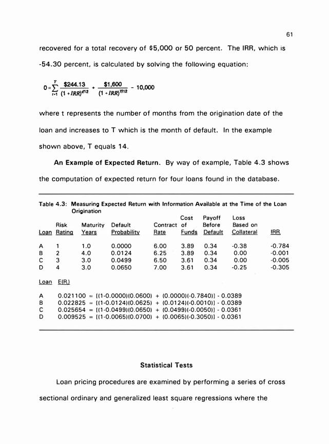
61

recovered for a total recovery of $5,000 or 50 percent. The IRR, which is

-54.30 percent, is calculated by solving the following equation:

O=E $244.13 + $1,600 - 10,000 ,., (1 + IRR)t112 (1 + IRR)7712

where t represents the number of months from the origination date of the

loan and increases toT which is the month of default. In the example

shown above, T equals 14.

An Example of Expected Return. By way of example, Table 4.3 shows

the computation of expected return for four loans found in the database.

Table 4.3: Measuring Expected Return with Information Available at the Time of the loan

Origination Cost Payoff Loss

Risk Maturity Default Contract of Before Based on

Loan Rating Years Probability Rate Funds Default Collateral

A 1 1.0 0.0000 6.00 3.89 0.34 -0.38

B 2 4.0 0.0124 6.25 3.89 0.34 0.00

c 3 3.0 0.0499 6.50 3.61 0.34 0.00

D 4 3.0 0.0650 7.00 3.61 0.34 -0.25

Loan E(Rl

A 0.021100 = [(1-0.0000)(0.0600) + (0.0000)(-0.7840)]- 0.0389

B 0.022825 = [(1-0.0124)(0.0625) + (0.0124)(-0.001 0)] - 0.0389

c 0.025654 = [(1-0.0499)(0.0650) + (0.0499)(-0.0050)]- 0.0361

D 0.009525 = [(1-0.0065)(0.0700) + (0.0065)(-0.3050)1- 0.0361

Statistical Tests

!.!lli

-0.784

-0.001

-0.005

-0.305

Loan pricing procedures are examined by performing a series of cross

sectional ordinary and generalized least square regressions where the

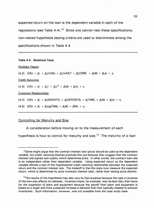
62

expected return on the loan is the dependent variable in each of the

regressions (see Table 4.4) .13 Since one cannot nest these specifications,

non-nested hypothesis testing criteria are used to discriminate among the

specifications shown in Table 4.4

Table 4.4: Statistical Tests

Portfolio Theorv

Credit Rationing

Customer Relationships

Controlling for Maturity and Size

A consideration before moving on to the measurement of each

hypothesis is how to control for maturity and size.14 The maturity of a loan

13Some might argue that the contract interest rate (price) should be used as the dependent variable, but credit rationing theories preclude this use because they suggest that the contract interest rate signals loan quality which determines price. In other words, the contract loan rate is an independent rather than dependent variable. Using expected return as the dependent variable affords a test of the hypothesized credit rationing relationship between the expected return and the contract interest rate. The tradeoff is that the tests now measure the expected return, which is determined by price (contract interest rate), rather than testing price directly.

14The results of the hypothesis may also vary by loan purpose because the type or purpose of the loan also affects its riskiness. Inventory loans, for example, may be less risky than loans for the expansion of plant and equipment because the payoff from plant and equipment is based on a larger and more sustained increase in demand than that typically needed to exhaust inventories. Such information, however, was not available from the case study bank.

63

affects its riskiness because the longer the maturity, the greater the

possibility that default might occur. Although maturity is incorporated by

differences in the cost of funds and default probabilities, it is included as an

independent variable in each equation specified to capture any residual

effects of the length of the loan on the expected return.

Different pricing practices are expected by size because larger loans

are generally associated with larger firms 1 l that often possess publicly

traded stocks which translates into more public information about the firms

and 2) that experience a more competitive loan environment because of the

national rather than regional scope of their market. Therefore, the original

amount of the loan is added to each regression.

Testing Mean-Variance Portfolio Theory

Mean-variance portfolio theory is considered in hypothesis 1 below.

Hypothesis 1 : Banks price commercial loans such that the expected return is linearly15 and positively related to the loan's individual risk and the loan's contribution of risk to the bank's entire loan portfolio.

The following equation considers whether mean-variance analysis and

portfolio theory are used in pricing:

Equation (4.2) is a cross-sectional test in which E(R;l represents the

bank's expected return from loan i, p, is the constant term, VAR; is the

16Linearity is assumed as a first approximation.

64

variance 16 for loan i, VARf is the variance squared and is used to test

whether the relationship is nonlinear, CORR; measures the correlation of an

industry's credit quality with the return on the bank's total loan portfolio, M;

is the number of days over which the loan is to be paid, A; is the original

amount of the loan, and E; is the error term.

The variable which represents the correlation between the return on the

case study bank's loan portfolio and the loan industry's credit quality

(CORR) warrants further explanation. The return on the bank's loan portfolio

is simply the interest income produced from the loan portfolio less charge-

offs net of recoveries all divided by the total loan balance.17 Credit quality

is the percentage change in the credit quality of the 4-digit standard

industrial classification (SIC) to which the loan belongs.18 The credit

quality measure was obtained from ZETA® Services which specializes in

measuring credit quality. Both the return on the bank portfolio and credit

quality measures are quarterly and were correlated for the 39 quarters from

the second quarter of 1983 through the fourth quarter of 1991.

18Even though the variance is measured from the expected return, which is the dependent variable, the relationship predicted by mean-variance analysis is not a certainty because the bank can misprice the loan by applying the wrong premium (contract interest rate less cost of funds), risk rating, or collateral reQuirements. In fact, loan D in Table 4.3 is mispriced relative to its variance. The variance of each loan in the table is: VARA = 0.00000, VAR8 = 0.479, VARc = 2.006, and VAR0 = 85.465. [Variances in the regressions are multiples by 100 to avoid the negative bias that would occur when numbers less than one are sQuared.]

17These data were obtained from the case study bank's Quarterly earnings reports.

181n some cases, a 4-digit SIC credit Quality measure was not available. Therefore, CORR was measured at the 3-digit SIC level for 102 observations and at the 2-digit SIC level for 1 18 observations.

65

The correlation between the bank's return on its loan portfolio and

credit quality provides a useful measure of portfolio pricing because the

lower correlations of returns between loans leads to lower variations in the

entire portfolio.19 Thus, if a loan's credit quality moves opposite that of the

case study bank's loan portfolio over time, the addition of this loan to the

portfolio could reduce the variability of the entire loan portfolio. Said

differently, the variation of an existing loan portfolio can be reduced by

adding loans of firms whose business cycle runs counter to that of the

bank's portfolio. The underlying concept is that a firm's credit quality is

most likely to deteriorate during business downturns. If the firm's business

cycle trough occurs counter to that of the bank's loan portfolio, then adding

the counter-cyclical firm's loan to the bank's portfolio can potentially reduce

the variation in the portfolio.

Because bankers are generally risk-averse (Flannery, 1985 and Hester

and Pierce, 1972), they are expected to place greater value on industries

that reduce the total variability of the return on their loan portfolio.

Moreover, "Because bank shareholders are willing to trade off some

expected profits in order to avoid uncertainty (and vice versa), the

diversification principle has an important implication for loan pricing"

(Flannery, 1985, p. 462). Consequently, it is hypothesized that bankers

discount the contract interest rate of loans whose industry is associated

19For a more detailed explanation of the role correlations play in portfolios, see pages 25 through 27.

66

with a relatively small or negative correlation (higher credit quality numbers

are associated with better credit quality). Hence, P4 is expected to be

positive.

Support for mean-variance analysis would be evident from a positive

and statistically significant P2 coefficient because the expected return should

increase as the variance increases. In addition, assuming a linear

relationship between risk and return, P3 is expected to be statistically

insignificantly different from zero. A joint hypothesis test (Yancey, Judge,

and Bock, 1981) would indicate thatP2>0 andP3=0. However, the

relationship between expected return and risk may not be linear. Therefore,

portfolio theory would be supported by P3 > 0. As noted above, portfolio

theory suggests a positive coefficient P4 since loans that decrease the

variance of the bank's loan portfolio are expected to be priced relatively

lower than other loans and hence should be associated with a lower

expected return. Finally, in this test as well as the others noted below, P5,

the coefficient which measures maturity, is expected to be positive because

longer maturities are generally associated with higher default rates.

Testing the Theory of Credit Rationing

The pricing implications of credit rationing theories are considered in

the following hypotheses:

Hypothesis 2a: Banks price commercial loans such that the expected return reaches a maximum at a particular rate and beyond that point declines relative to the contract interest rate.

Hyoothesis 2b: The expected return on collateralized loans is

greater than the expected return on noncollateralized loans.

67

The following equation considers the implications from the theory of

credit rationing in pricing commercial loans:

where i ; represents the contract interest rate. In this case, the contract

interest rate on the loan acts as a signal that, after a particular point, causes

the expected return on the loan to fall (Stiglitz and Weiss, 1981 ) . Therefore,

a statistically significant positive /12 and negative {13 would support credit

rationing because the relationship between the expected return and interest

rates form a parabola. In this case, a joint hypothesis would indicate that

{12 > 0 and /13 < 0. If only /13 is statistically significantly different from zero

and positive, this result would not provide evidence against credit rationing

because a bank that properly rations credit based on default risk would

decline loans at the point where adverse selection and moral hazard

outweighs the possible increased returns from risk.

A secondary question raised in credit rationing literature is whether

collateral intensifies moral hazard (Stiglitz and Weiss, 1981) or reduces it

(Guttentag and Herring, 1984). 20 This question is investigated with an

analysis of the means of the expected return on loans when loans are

20Moral hazard, which means that borrowers take on more risk than agreed upon in the contract, may still occur if the loan is paid in full. In such a case, the borrower who took on a riskier project was successful. It is unlikely that this happened enough times to significantly bias the results, particularly since the sample data include a business cycle downturn.

68

grouped based on whether the loan terms include collateral.

Testing Customer-Relationship Theories

The pricing implications of customer relationships are considered in the

following hypotheses:

Hypothesis 3a: Banks price commercial loans such that the expected return they earn from commercial loan customers who contribute most to their long-term profitability is lower in the short run than that which they receive from nonpreferred customers.

Hypothesis 3b: The expected return a bank earns from commercial loan customers who have been with the bank for a long period of time is greater than that for new customers.

The following equation is used to test the degree to which customer

relationships are important in pricing loans as defined by Hodgman (1961

and 1963) and Kane and Malkiel (1965):

Sharpe (1990), however, suggests an opposing model with regard to time:

In the above equations, SIZE; is the current size of account i, GROWTH; is

the future growth prospects for account i, DEPOSITS; is the total deposits

for account i, and TIME; is the total days customer i has dealt with the bank.

The measurement of the variables in equations (4.4) and (4.5) is fairly

straightforward. GROWTH is the projected growth rate of industry

69

employment from 1990 through 2005 (U.S. Department of Labor, 1992). 21

Projections were generally applied at the three-digit standard industrial

classification level. 22 DEPOSITS is the dollar value of deposits. TIME is the

number of days since the customer opened his or her first loan or deposit

account with the bank.

Support for the importance of customer relationships in pricing would

be indicated by a negative coefficient for DEPOSITS and GROWTH. Also, a

negative coefficient for TIME would provide evidence for the importance of

customer relationships as suggested by Hodgman and Kane and Malkiel; but

a positive coefficient would support Sharpe's "informationally captured"

notion. A further test of Sharpe's concept is provided in equation (4.5)

where TIME is transformed by using a log function because the relationship

between the expected return on the loan relative to the length of the

relationship is expected to be convex: the interest rate on loans for new

customers are discounted while longer customers are charged a higher rate.

Non-Nested Tests

The explanatory power of the models that represent the theories above

are compared by using the non-nested J-test (Davidson and MacKinnon,

2'These projections are used because they were available in 1 992 when the loans in the database were made. Output is a better measure of industry growth, but it is not available from a public source at the level of detail used in this study.

221f a growth projection is not available at the 3-digit SIC level, then the projection for the

relevant 2-digit level is used. One hundred twenty observations required projections at the 2-digit level.

1981) and Cox test (Cox, 1961 and 1962 and Pesaran, 1974). 23 These

tests are explained through the following two hypothesis:

H0: Y = XPx + Ux H,: y = xp, + u,

The J-test is performed by first separately performing the regressions

specified by theories "X" and "Z" and saving the fitted values (Yx and Yz)

70

from the regressions. The second step involves re-estimating the regression

concerning theory X and including Yz from the second equation as an

independent variable. If the coefficient on y, is significantly different from

zero, then the null hypothesis that model X provides the greatest

explanatory power is rejected in favor of H,. This process is repeated to test

whether theory X provides additional information to theory Z by reversing

the roles of H0 and H,. It is possible that both models will be rejected as the

most informative set of regressors.

The Cox-test is a stronger nonnested test because it takes into account

the residuals as well as the predicted values of the competing theories. The

explanation of this test is based on the following two regression models

(Greene, 1993, pp. 222-225):

Mx: Y = XPx + Ux, Mz: Y = Z/3z + Uz,

Ux - N(O,a-21"), Uz - N(O,w210),

where y is the (n X 1) vector of observations on the dependent variable, X

and Z are (n X kxl and (n X kz) observation matrices for the regressors of

23Models are non-nested if the regressors of one model cannot be expressed as a linear combination of the regressors of the second model (Pesaran, 1987).

71

models Mx and Mz, Px and Pz are the (kx X 1) and (kz X 1) regression

coefficient vectors, and Ux and Uz are the (n X 1) error vectors, and I" is the

identity matrix of order n.

The information needed to calculate the Cox statistic for testing the

hypothesis that X provides greater explanatory power than Z is obtained as

by-products of computing the following four least square regressions. (See

Table 4.5 for a summary of this procedure.) First, the regression model Mx

is run to obtain the fitted value (Xb) and the mean-squared residual (s�). The

value for s� is set aside to be used in the Cox statistic. Second, Xb is used

as the dependent variable with the independent variables of the competing

model. This regression is performed in order to obtain the residuals (M,Xb)

and the sum of squared residuals (b'X'MzXb) which are set aside to be used

in the Cox statistic. Third, the residuals M.Xb are used as the dependent

variable with the independent variables of the regressors for theory X. The

value for the sum of squared residuals (b'X'MzlMx(MzXb) from this

regression is set aside to be used in the Cox statistic. Finally the regression

model M. is run to obtain its mean-squared residual (s�).

The above information is used to compute two more statistics that

allow the measurement of the Cox statistic (q). First s�x is computed as s�

+ ( 1 /n)b'X'MzXb. Second c12 is computed as

2 2

c12 = !!.tn[ s,

1 = !!.tn[2] 2 s! +(1/n)b1X1M�b 2 s!

Now, the hypothesis that X is the correct set of regressors and Z is not is

tested by the following statistic:

Table 4.5: Definition of Variables Needed to Compute the Cox-Statistic

Regression Models: Mx: y = XPx + Ux, Mz: Y = Z/iz + Uz,

C12 Cox Statistic = q= ------

(Est. Var(c12])112

where

Ux - N(O,ifl"), Uz - N(O,w21nl.

s� = e�ez/n = mean-squared residual in the regression of y on Z

s� = e�ex/n = mean-squared residual in the regression of y on X

Xb = fitted values in the regression of y on X

MzXb = residuals in a regression of Xb on Z

b'X'MzXb = sum of squared residuals in the regression of Xb on Z

six = s� + (1/n)b'X'MzXb

(b'X'MzlMx(MzXbl = sum of squared residuals in the regression MzXb on X

Mx = I - X(X'X)'1 X'

72

where a large value of q in a standard normal table is evidence against the

null hypothesis that X is the correct set of regressors.

73

As noted earlier, the nonnested tests consider the explanatory power of

one hypothesis against another. Since three hypotheses are considered in

this study, the tests must be computed for three pairs: 1) portfolio versus

credit rationing, 2) portfolio versus customer relationships, and 3) credit

rationing versus customer relationships. Failing to reject one hypothesis

does not rule out the possibility that the other hypotheses contribute

information about pricing.

CHAPTER V

PRESENTATION OF EMPIRICAL FINDINGS

This chapter contains the empirical results of the tests presented in

the previous chapter. The results provide evidence consistent with credit

rationing and customer relationship theories. Both the nonnested J-test and

the Cox test indicate that the specification used for the credit rationing

model provides more information about the expected return on loans than

the specification used for the customer relationship model.

The specification used to test portfolio theory provides statistically

significant results, but of the wrong sign: the expected return on loans

decreases as risk (variance) increases. Further tests were performed

because of this surprising result, and the additional tests suggest that loan

pricing at the case study bank might not adequately account for losses

associated with the possibility of default. In other words, default is more

likely with high variability of return which suggests that the case study bank

might be mispricing its loans.

Finally, the impact of collateral on loan pricing is considered. The

results indicate that the expected return associated with collateralized loans

is lower than that for loans without collateral. These results are consistent

74

75

with Boot, Thakor, and Udell (1991) who argue that firms use collateral to

obtain more favorable loan terms.

Testing for Heteroscedasticity

Most of the theories tested in this chapter were positively evaluated

for heteroscedasticity. A priori evidence and examination of the residual

patterns of the dependent variables suggest the original amount of the loan

(A) is causing the heteroscedasticity problem.1 As shown in Table 5.1, the

Park-Giejser test statistically verifies that the original amount of the loan is

contributing to the heteroscedasticity. 2

Even though the data are heteroskedastic, they are not adjusted to

reduce the heteroskedasticity because the nonnested tests used in this

chapter require ordinary least squares regression results. Moreover, even in

the presence of heteroskedasticity, the parameter estimates remain unbiased

and consistent. 3 As a result, the coefficients can be interpreted

1A priori, the variance of the loan amount is expected to increase around the expected return as loans became smaller because smaller loans are associated with less information and thus are probably priced with greater variation. In contrast, larger loans typically originate from larger firms, which often are traded publicly. The larger loans are probably priced more accurately because of the additional information.

2The Park-Giejser statistics shown in Table 5.1 are obtained by first regressing the model specification with ordinary least squares in order to obtain the residuals which are used as a proxy for the variances. The log of the squared residuals from the regression is used as the dependent variable in an ordinary least squares regression where the log of the loan amount (A) is the independent variable. The hypothesis that A is contributing to the heteroskedasticity in the data is accepted if its coefficient is statistically significantly different from zero.

3When data are heteroskedastic, their variances are not constant over observations. As a result, ordinary least squares places more weight on the observations with large variances

(continued ... )

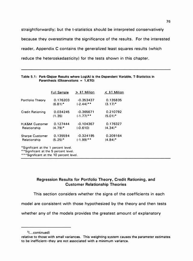
76

straightforwardly; but the t-statistics should be interpreted conservatively

because they overestimate the significance of the results. For the interested

reader, Appendix C contains the generalized least squares results (which

reduce the heteroskedasticity) for the tests shown in this chapter.

Table 5.1: Park-Giejser Results where Log(Al is the Dependent Variable, T -Statistics in Parenthesis (Observations = 1,6701

Full SamQie > $1 Million < $1 Million

Portfolio Theory 0.176203 -0.353437 0.135835

(6.811* (-2.441** (3. 1 71*

Credit Rationing 0.034245 -0.365671 0.210792

(1.351 (-1.771** (5.011*

H,K&M Customer 0.127444 -0.104367 0.176327

Relationship (4.791* (-0.6101 (4.341*

Sharpe Customer 0.135594 -0.324195 0.209164

Relationship (5.251* (-1 .991** (4.841*

• Significant at the 1 percent level. • • Significant at the 5 percent level. • • • Significant at the 10 percent level.

Regression Results for Portfolio Theory, Credit Rationing, and

Customer Relationship Theories

This section considers whether the signs of the coefficients in each

model are consistent with those hypothesized by the theory and then tests

whether any of the models provides the greatest amount of explanatory

3( ••• continued)

relative to those with small variances. This weighting system causes the parameter estimates

to be inefficient--they are not associated with a minimum variance.

77

power. The results shown in this section are not consistent with the notion

that banks price loans relative to portfolio theory. However, the results are

consistent with credit rationing and customer relationship theories. The

three theories are considered in turn.

Portfolio Theory

The test of the portfolio specification used in this study provides no

evidence that loan prices are positively related to risk. As shown in column

one of Table 5.2, the coefficient associated with VAR is statistically

significantly different from zero and inversely related to the expected return

on the loan while the hypothesis calls for a positive coefficient. The

coefficient for V AR2 is also negative, but it is not statistically significant.

Although these results are contrary to basic financial theory, they are

suggested by banking industry observers who say that banks price their best

customers' paper too low and their worst customers' paper too high.4

The definition of expected return and variance used in this study is set

forth by portfolio theory. However, the variables used to calculate the

loan's expected return and variance are broader than those used by banks.

Specifically, the expected return is based on the risk rating the bank applies

to the loan, the type of collateral associated with the loan, and the recovery

amount of the loan if it defaults--an approach that explicitly incorporates

4For example, see Foss (1992), Portfolio Valuation Handbook (1989) and Rose (1992).

78

Table 5.2: Ordinary Least Squares Results where the Dependent Variable is the Expected Return

on the Loan, T -Statistics In Parenthesis (Observations = 1 ,6701

Portfolio Credit Customer Relationships Theory Rationing H.K&M �

Intercept 3.547293 -2.067980 3.399496 4.038350

(61.141* (-4.71 )* (37.381* (18.00)*

VAR -0.015015

(-33.09)*

VAR2 -0.000000

(-0.01)

CORR 0.537148

(2.27)**

A -0.000000 -0.000000 -0.000000 -0.000000

(-16.29) * (-3.04)* (-12.231* (-13.23)*

M -0.001293 -0.002956 -0.002458 -0.002362

(-18.77)* (-43.10)* (-32.25)* (-31.34)*

RATE 0.849947

(7.45)*

RATE2 -0.006419

(-0.89)

GROWTH 0.003428

(1.721***

DEPOSITS -0.000000

(-6.041*

TIME -0.000015

(-0.87) I

Log(TIMEI -0.105007 I (-3.42)*

Adjusted R2 0.64 0.58 0.42 0.40

F-Statistic 600.13* 569.67* 235.76* 372.91 *

• Significant at the 1 percent level. • • Significant at the 5 percent level. • • • Significant at the 1 0 percent level.

79

more information than most banks probably use to price loans.5

Consequently, the calculation of the expected return and variance may be

biasing the results. Theoretically, however, the contract interest rate and

the cost of funds used by banks to price loans should implicitly incorporate

default probability and recovery rates. The difference between the definition

used in this study and that which banks use allows further tests that shed

light on the surprising results from portfolio theory. These tests are

presented later in this chapter.

The second measure of portfolio pricing, CORR, is positive and

statistically significantly different from zero at the 5 percent level. This

result should be discounted, however, because t-statistics are overestimated

in the presence of heteroscedasticity. CORR measures the correlation

between the return on the bank's loan portfolio and the change in the credit

worthiness of firms in the same industry group. The positive relationship

suggests that the pricing practices of the case study bank might have taken

into consideration the correlation between the industry in which the

borrower is a member and the bank's total loan portfolio. However, the

heteroscedastic-consistent results shown in Appendix C indicate that the

coefficient is not statistically significantly different from zero. The

insignificance of this variable is consistent with the banking literature which

indicates that banks have only recently begun to consider the impact on

6The loan pricing examples shown in Table 8.1 of Appendix 8, for example, do not consider the impact of collateral recovery in loan pricing.

80

individual loans of the return to their total loan portfolio. 6

The variables, A and M were included in each of the regressions to

control for the size and maturity of the loans. Both variables were

statistically significantly different from zero and inversely related to the

expected return on the loans in each regression specified in Table 5.2. In

fact, this relationship held true for every regression that was run for this

study irrespective of how the sample was subdivided. These findings

provide strong support that the expected return increases as the loan size

and maturity decreases.

The relationship between the expected return and the amount of the

loan can be explained from several different points of view. First, smaller

loans may be associated with smaller firms that are considered riskier than

larger firms. Second, as suggested by customer relationship theories, larger

loans contribute more to the bank's long-run profits. Thus, they are charged

less in the short run in an attempt by the bank to retain the preferred

customer. Third, increased competition for larger loans might have driven

down the expected return for these preferred loans. The increased

competition includes banks as well as other financial markets, such as

commercial paper. Finally, this finding is also consistent with the theory

that large loans are associated with relatively lower interest rates because of

economies of scale.

6For example, see Gallinger and Morgan (1993), Larr and Stampleman (1993), and Mersman (1991 ).

81

The regressions performed for this study also provide strong support

that the expected return on loans is inversely related to the maturity of the

loan. This result is opposite the expected result: longer loans are

associated with higher returns because they possess a greater probability of

default. The bond defaults shown in Table 4.2 clearly show this relationship

between default and time. According to officials at the case study bank,

however, short-term loans are preferred over long-term loans.

Consequently, only the bank's best customers are granted loans with

relatively long maturities. As suggested by customer relationship theories,

preferred customers are granted lower interest rates. The lower interest

rates translate into lower expected returns for the bank.

Credit Rationing

The regression results for credit rationing specification shown in Table

5.2 are consistent with the notion that banks control risk by denying credit

to the riskiest borrowers and use the contract interest rate as a signal of a

borrower's riskiness. The theory of credit rationing, which assumes

asymmetric information, suggests that beyond a maximum interest rate,

banks do not lend because higher rates do not compensate for adverse

selection and moral hazard.

Results consistent with credit rationing can be found in three different

relationships. First, weak support for credit rationing would be indicated by

an upward sloping contract interest rate� Second, if the bank does not

82

ration credit properly, a parabolic relationship would exist between the

expected return on the loan and the contract interest rate. Third, a negative

sign on the coefficient of the squared interest rate would also support credit

rationing by indicating the relationship is nonmonotonic and loans are not

extended beyond a certain interest rate.

The results shown in column two of Table 5.2 provide weak support

for credit rationing. The contract interest rate (RATE) is positive and

statistically significantly different from zero. However, a statistically

insignificant relationship exists between RATE2 and the expected return. (A

joint test for RATE and RA TE2 was rejected.)

Customer Relationship Theories

Two model specifications of customer relationships are considered in

Table 5.2. The first model is denoted H,K&M because it relies on theories

presented by Hodgman ( 1961) and Kane and Malkiel ( 1965). The second

model specification is based on Sharpe ( 1990).

According to the H,K&M theories of customer relationships, certain

customer characteristics contribute more to a bank's long-term profitability

than others. Thus, the relevant marginal calculation of granting a loan is not

whether the additional expected profit from making the loan outweighs the

increased risk, but the importance of the characteristics of the customer to

the bank's long-run profits. Specifically, large accounts are preferred to

small ones, growing accounts are more valuable than declining ones, larger

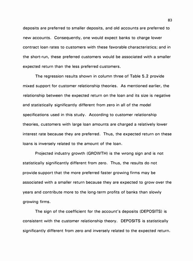
83

deposits are preferred to smaller deposits, and old accounts are preferred to

new accounts. Consequently, one would expect banks to charge lower

contract loan rates to customers with these favorable characteristics; and in

the short-run, these preferred customers would be associated with a smaller

expected return than the less preferred customers.

The regression results shown in column three of Table 5.2 provide

mixed support for customer relationship theories. As mentioned earlier, the

relationship between the expected return on the loan and its size is negative

and statistically significantly different from zero in all of the model

specifications used in this study. According to customer relationship

theories, customers with large loan amounts are charged a relatively lower

interest rate because they are preferred. Thus, the expected return on these

loans is inversely related to the amount of the loan.

Projected industry growth (GROWTH) is the wrong sign and is not

statistically significantly different from zero. Thus, the results do not

provide support that the more preferred faster growing firms may be

associated with a smaller return because they are expected to grow over the

years and contribute more to the long-term profits of banks than slowly

growing firms.

The sign of the coefficient for the account's deposits (DEPOSITS) is

consistent with the customer relationship theory. DEPOSITS is statistically

significantly different from zero and inversely related to the expected return.

84

Similar to the loan size argument, these customers are granted a lower

contract rate because of their long-term contribution to the bank's profits. 7

The length of the customer relationship is not statistically significantly

different from zero but negatively related to the loan's expected return.8

According to customer relationship theories, longer-term relationships

provide greater opportunity for profits. Thus, these customers are charged

less in the short run.

The second model specification of the customer relationship theory

(Sharpe, 1990) simply states that bank customers become informationally

captured by the bank that provides it with loans. Because of asymmetric

information, the bank that loans to a customer learns more about that

customer over time than do other banks. Thus, the bank that loans to the

high quality firm offers it a lower rate, when compared with other banks; but

the contract rate would be even lower if competing banks knew the true

high quality of the customer. As a result, banks charge their better

customers--those that become informationally captured--a relatively high rate

7Customer relationship theories also suggest that customers with less deposit variability are preferred. Deposit variability (DEPSTE) is not included in the customer relationship specification because only 899 loans were associated with the data required to calculate deposit variability. A separate customer relationship regression was run with the 899

observations and it indicates that DEPSTE is statistically significantly different from zero at the 1 percent level. (DEPOSITS were not included in this regression because of multicollinearity.) Moreover, DEPSTE is negatively related to the expected return. The result is opposite that suggested by customer relationship theory: customers with lower deposit volatility are preferred customers who receive a lower contract interest rate than nonpreferred customers.

8The form of this variable may be misspecified because the Sharpe customer relationship

results indicate TIME is inversely and statistically significantly related to the expected return when TIME is in log form.

85

compared with new customers.

The results shown in the fourth column of Table 5.2 do not support

Sharpe's theory. The length of the customer relationship (log(TIME)) is

statistically significant but inversely related to the loan's expected return.

J-Test and Cox-Test

The J-test and Cox-test consider whether any of the theories tested in

this study provide significantly more explanatory power in commercial loan

pricing. (See pages 69 through 73 for a further explanation of non-nested

tests.) As mentioned earlier, the model specification for portfolio theory and

Sharpe's (1990) customer relationship theories provide coefficients that are

statistically significantly different from zero, but signs opposite those

hypothesized by their respective theories (see Chapter IV). Because these

model specifications fail to explain loan pricing as proposed by theory, they

are not included in the non-nested tests.

Table 5.3: Results of J-Test: Predicted Values for Re-estimated Equations, T-Statistics in Parenthesis

Dependent Variable: Expected Return on Loans

H0: Credit Rationing H,: H,K&M Customer Relationship

H0: H,K&M Customer Relationship H,: Credit Rationing

• Significant at the 1 percent level. • • Significant at the 5 percent level.

Predicted Values for: Credit Rationing

0.992941

(25.57).

Customer Relationships H.K&M

0.209541

(1 . 64)

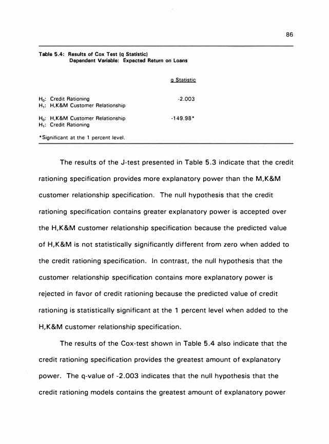
86

Table 5.4: Results of Cox Test (q Statistic) Dependent Variable: Expected Return on Loans

H0: Credit Rationing H,: H,K&M Customer Relationship

H0: H,K&M Customer Relationship H,: Credit Rationing

• Significant at the 1 percent level.

a Statistic

-2.003

-149.98*

The results of the J-test presented in Table 5.3 indicate that the credit

rationing specification provides more explanatory power than the M,K&M

customer relationship specification. The null hypothesis that the credit

rationing specification contains greater explanatory power is accepted over

the H,K&M customer relationship specification because the predicted value

of H,K&M is not statistically significantly different from zero when added to

the credit rationing specification. In contrast, the null hypothesis that the

customer relationship specification contains more explanatory power is

rejected in favor of credit rationing because the predicted value of credit

rationing is statistically significant at the 1 percent level when added to the

H,K&M customer relationship specification.

The results of the Cox-test shown in Table 5.4 also indicate that the

credit rationing specification provides the greatest amount of explanatory

power. The q-value of -2.003 indicates that the null hypothesis that the

credit rationing models contains the greatest amount of explanatory power

87

should be accepted over the alternative hypothesis that the H,K&M

customer relationship theory provides the greatest amount of explanatory

power. When the hypotheses are switched, the q-statistic of -149.98

indicates that the null hypothesis of the H,K&M customer relationship theory

should be rejected in favor of credit rationing.

Further Tests of loan Pricing

The remainder of this chapter considers three additional questions

related to loan pricing. First, did the calculation of expected return account

for the lack of evidence in this study that banks price loans relative to risk?

Second, are collateralized loans priced differently than noncollateralized

loans? Finally, are loans from larger firms, which are usually associated with

more information, priced differently than loans from smaller firms, which are

usually associated with less information?

Calculation of Expected Return

The definition of the expected return on the loan used in this study is

broader than that used in previous studies of loan pricing and is also broader

than that used by most banks. In earlier studies, the premium had been

used to measure a bank's return on its loans, mainly because further

information was not available (for example, Berger and Udell, 1989).

However, the premium does not explicitly take into account such factors as

the default probability or the recovery on the loan in the case of default

88

because of the subjective nature of risk evaluations (see Table 5.5).9 If, as

suggested by industry observers, banks do not currently incorporate the

default probability related to loans (Altman, 1993), then a regression which

Table 5.5: Two Ways to Determine the Return on a Loan

Expected Return

Calculation: ( 1-d)(i-i"} + (d)(IRR-i"}

• Default Probability (d) - determined by applying the loan risk rating and the maturity of the loan to corporate default tables (see pages 57 and 58 for a more detailed explanation of this process).

• Risk Rating - an integer from one to eight where one is assigned to the least risky loans. Ratings are assigned by the bank's account managers. The ratings are based on financial measures and other firm-specific information.

• Premium (i-i"} - defined below as the contract interest rate less the cost of funds.

• Internal Rate of Return (IRR) - the return on the loan if default occurs. It assumes default occurs aher 34 percent of the loan has been paid. The total recovery rate of the loan is dependent on the type of collateral associated with the loan.

Premium

Calculation: (i-i.)

• Cost of Funds (i') - based on the yield of a government bond with a maturity eQual to that of the proposed commercial loan plus a factor which covers the cost of insurance and brokerage fees.

• Rate (i) - the contract interest rate on the loan, which is based on the risk rating but does not estimate recovery in the case of default.

uses the premium instead of the expected return as the dependent variable

will be associated with an increased error variance.

9Banks can calculate default probabilities and the expected recovery on loans in the case of default. However, the historical data needed to make such calculations have not been gathered and stored by banks.

89

The first column of Table 5.6 presents the results of the portfolio

theory regression as specified for this study where the expected return is the

dependent variable. The second column contains the results when the

premium is used as the dependent variable. The statistical significance and

Table 5.6: Reconsidering the Portfolio Theory Specification Ordinary Least Squares Results. T -Statistics in Parenthesis (Observations = 1,670)

De[!eng!;lnt V§!ri§!ble� Ex[!ected Return Premium Ex[!ected Return Premium

Intercept 3.547293 3.192322 4.031320 1.418214

(61.14)* (63.13)* (17.50)* (9.20)*

VAR -0.015015 0.000337

(-33.09)* (0.85)

VAR2 -0.000000 0.000014

(-0.01) (9.70)*

RISK -0.190320 0.455177

(-3.30)* (11.86)*

CORR 0.537148 0.332567 0.294687 0.559346

(2.27)** ( 1.61) (0.96) (2.73)*

A -0.000000 -0.000000 -0.000000 -0.000000

(-16.28)* (-17.45)* (-13.58)* (-14.90)*

MATURITY -0.001293 -0.000157 -0.002394 0.000108

(-18.77)* (-2.62)* (-31.74)* (2.14)**

Adjusted R2 0.64 0.20 0.40 0.22

F-Statistic 600.13* 84.56* 279.74* 116.17*

• Significant at the 1 percent level. .. Significant at the 5 percent level. • • • Significant at the 1 0 percent level.

signs of the coefficients differ. When PREMIUM is used as the dependent

variable, V AR is positive and insignificant while V AR2 is positive and

statistically significantly different from zero. These results suggest that as

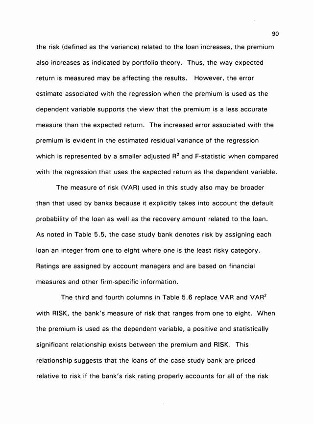
90

the risk (defined as the variance) related to the loan increases, the premium

also increases as indicated by portfolio theory. Thus, the way expected

return is measured may be affecting the results. However, the error

estimate associated with the regression when the premium is used as the

dependent variable supports the view that the premium is a less accurate

measure than the expected return. The increased error associated with the

premium is evident in the estimated residual variance of the regression

which is represented by a smaller adjusted R2 and F-statistic when compared

with the regression that uses the expected return as the dependent variable.

The measure of risk (V AR) used in this study also may be broader

than that used by banks because it explicitly takes into account the default

probability of the loan as well as the recovery amount related to the loan.

As noted in Table 5.5, the case study bank denotes risk by assigning each

loan an integer from one to eight where one is the least risky category.

Ratings are assigned by account managers and are based on financial

measures and other firm-specific information.

The third and fourth columns in Table 5. 6 replace V AR and V AR2

with RISK, the bank's measure of risk that ranges from one to eight. When

the premium is used as the dependent variable, a positive and statistically

significant relationship exists between the premium and RISK. This

relationship suggests that the loans of the case study bank are priced

relative to risk if the bank's risk rating properly accounts for all of the risk

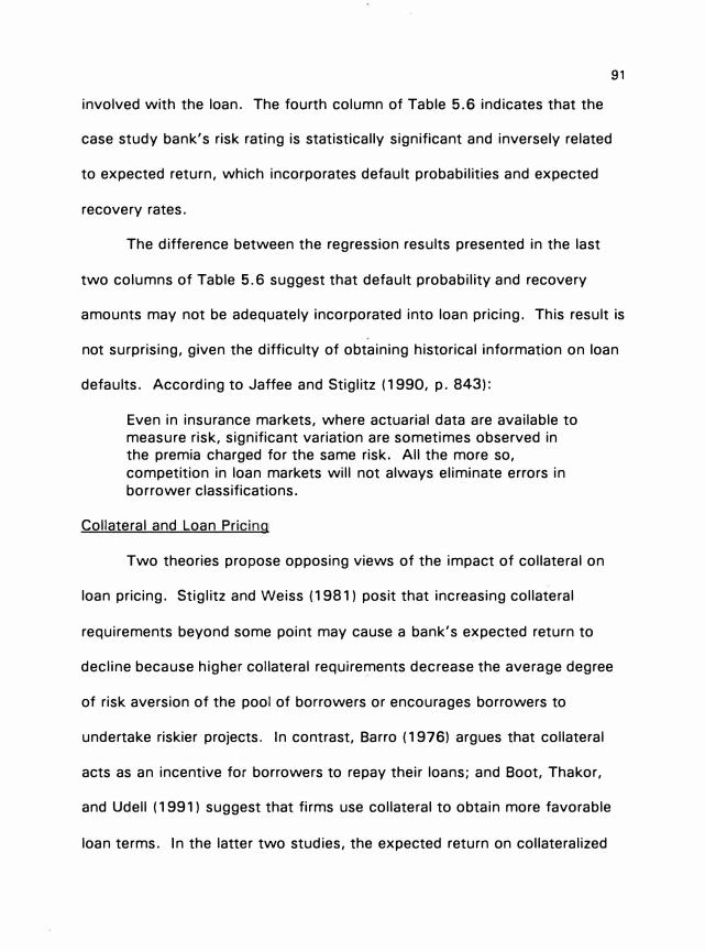
91

involved with the loan. The fourth column of Table 5.6 indicates that the

case study bank's risk rating is statistically significant and inversely related

to expected return, which incorporates default probabilities and expected

recovery rates.

The difference between the regression results presented in the last

two columns of Table 5.6 suggest that default probability and recovery

amounts may not be adequately incorporated into loan pricing. This result is

not surprising, given the difficulty of obtaining historical information on loan

defaults. According to Jaffee and Stiglitz (1990, p. 843):

Even in insurance markets, where actuarial data are available to measure risk, significant variation are sometimes observed in the premia charged for the same risk. All the more so,

competition in loan markets will not always eliminate errors in borrower classifications.

Collateral and Loan Pricing

Two theories propose opposing views of the impact of collateral on

loan pricing. Stiglitz and Weiss ( 1981) posit that increasing collateral

requirements beyond some point may cause a bank's expected return to

decline because higher collateral requirements decrease the average degree

of risk aversion of the pool of borrowers or encourages borrowers to

undertake riskier projects. In contrast, Sarro ( 1976) argues that collateral

acts as an incentive for borrowers to repay their loans; and Boot, Thakor,

and Udell (1991) suggest that firms use collateral to obtain more favorable

loan terms. In the latter two studies, the expected return on collateralized

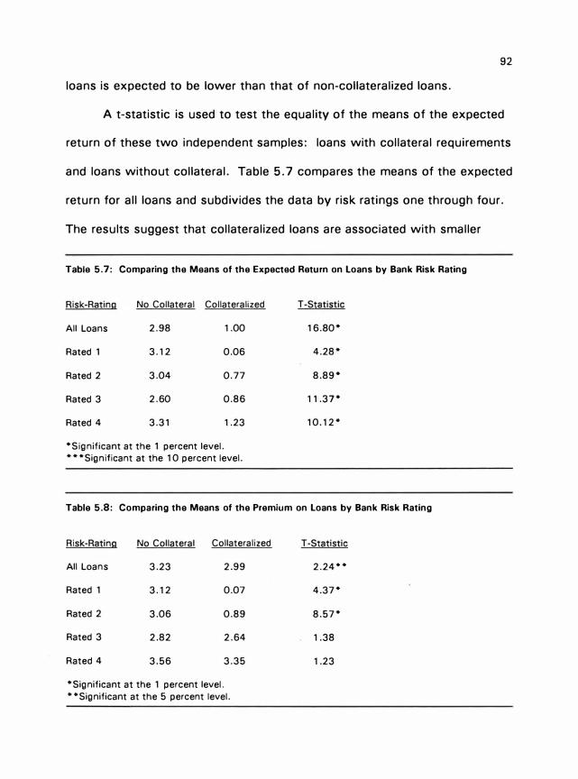
92

loans is expected to be lower than that of non-collateralized loans.

A t-statistic is used to test the equality of the means of the expected

return of these two independent samples: loans with collateral requirements

and loans without collateral. Table 5. 7 compares the means of the expected

return for all loans and subdivides the data by risk ratings one through four.

The results suggest that collateralized loans are associated with smaller

Table 5.7: Comparing the Means of the Expected Return on Loans by Bank Risk Rating

Risk-Rating No Collateral Collateralized T -S!atistic

All Loans 2.98 1.00 16.80*

Rated 1 3.12 0.06 4.28*

Rated 2 3.04 0.77 8.89*

Rated 3 2.60 0.86 11.37*

Rated 4 3.31 1.23 10.12.

*Significant at the 1 percent level.

• • *Significant at the 10 percent level.

Table 5.8: Comparing the Means of the Premium on Loans by Bank Risk Rating

Risk-Rating No Collateral Collateralized T -Sta!istic

All Loans 3.23 2.99 2.24**

Rated 1 3.12 0.07 4.37*

Rated 2 3.06 0.89 8.57*

Rated 3 2.82 2.64 1.38

Rated 4 3.56 3.35 1.23

*Significant at the 1 percent level.

• *Significant at the 5 percent level.

93

expected returns than noncollateralized loans. In other words, collateral is

associated with a higher expected payback and thus lower perceived risk.

These results support Barra, and Boot, Thakor, and Udell. This relationship

held true for the total sample as well as each individual risk rating.

A comparison of the means of the premium on loans provided similar

results. As shown in Table 5.8, loans with collateral were associated with

statistically significantly smaller premiums than those without collateral.

This relationship, however, was not significant for loans with risk ratings

three and four.

Firm Size and Loan Pricing

Large firms are expected to be associated with relatively more

information than small firms because the larger firms are more often publicly

traded. Unfortunately, the size of the firm associated with each loan in the

database is not available. However, the study makes the same assumption

used by. previous studies that larger loans are associated with larger firms.

Consequently, the regressions are recalculated for portfolio theory, credit

rationing, and customer relationships where the sample is divided between

loans greater than or equal to $1 million and those that are less than $1

million (see Tables 5.9 through 5.12).

The regressions that are subdivided by size provide results similar to

those already reported in the case of customer relationships as defined by

Sharpe (Table 5.2). The regression results of the subdivided data do not

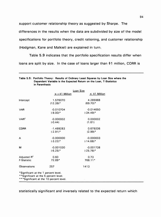
94

support customer relationship theory as suggested by Sharpe. The

differences in the results when the data are subdivided by size of the model

specifications for portfolio theory, credit rationing, and customer relationship

(Hodgman, Kane and Malkiel) are explained in turn.

Table 5.9 indicates that the portfolio specification results differ when

loans are split by size. In the case of loans larger than $1 million, CORR is

Table 5.9: Portfolio Theory: Results of Ordinary Least Squares by Loan Size where the

Dependent Variable is the Expected Return on the Loan, T-Statistics

in Parenthesis

Loan Size > =$1 Million < $1 Million

Intercept 1.576070 4.285988

(12.39). (69.70)•

VAR -0.010704 -0.014650

(-9.00)• (-34.49)•

VAR2 -0.000002 0.000002

(-0.44) (1.61)

CORR -1.499283 0.679206

(-2.91)• (2.99)•

A -0.000000 -0.000003

(-3.22)• (-14.68)•

M -0.001030 -0.001738

(-6.25)• (-25.78)•

Adjusted R2 0.60 0.73

F-Statistic 72.89. 768.11.

Observations 257 1413

• Significant at the 1 percent level. • • Significant at the 5 percent level. • • • Significant at the 1 0 percent level.

statistically significant and inversely related to the expected return which

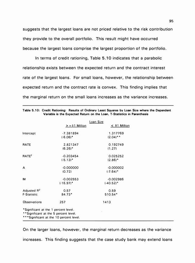
95

suggests that the largest loans are not priced relative to the risk contribution

they provide to the overall portfolio. This result might have occurred

because the largest loans comprise the largest proportion of the portfolio.

In terms of credit rationing, Table 5.10 indicates that a parabolic

relationship exists between the expected return and the contract interest

rate of the largest loans. For small loans, however, the relationship between

expected return and the contract rate is convex. This finding implies that

the marginal return on the small loans increases as the variance increases.

Table 5.10: Credit Rationing: Results of Ordinary Least Squares by Loan Size where the Dependent

Variable is the Expected Return on the Loan, T-Statistics in Parenthesis

Loan Size > = $1 Million < $1 Million

Intercept -7.381894 1.317769

(-6.06)* (2.04)*.

RATE 2.821347 0.192749

(6.26)* (1.27)

RATE2 -0.203454 0.025252

(-5.13)* (2.86)*

A -0.000000 -0.000002

(0.72) (-7.64)*

M -0.002553 -0.002986

(-16.97)* (-40.52)*

Adjusted R2 0.57 0.59

F-Statistic 84.73* 510.54*

Observations 257 1413

• Significant at the 1 percent level. • • Significant at the 5 percent level. • • • Significant at the 1 0 percent level.

On the larger loans, however, the marginal return decreases as the variance

increases. This finding suggests that the case study bank may extend loans

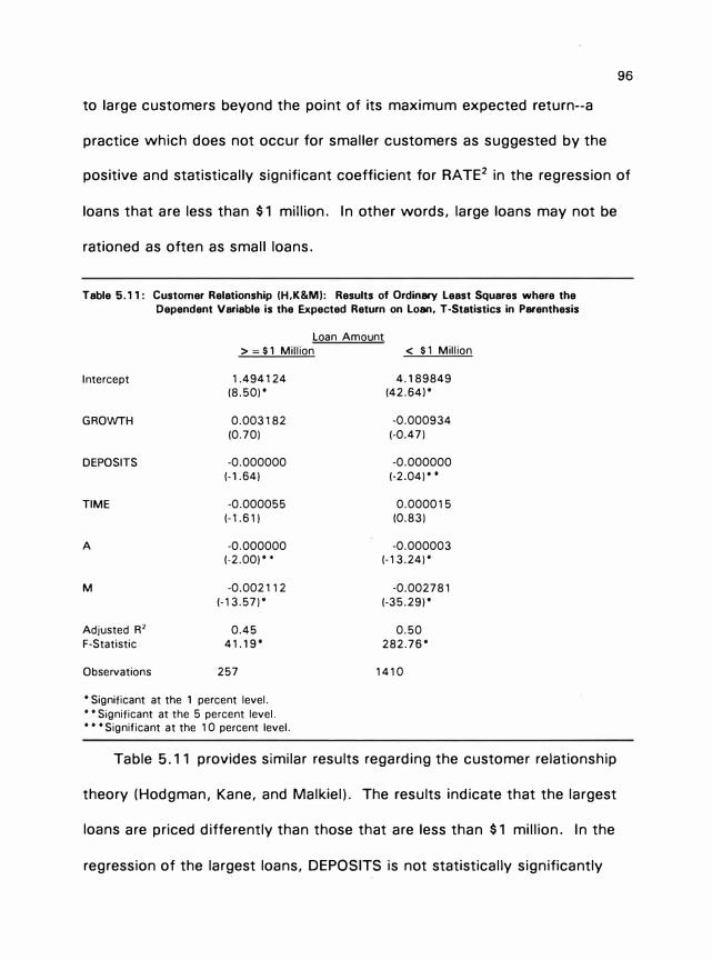
96

to large customers beyond the point of its maximum expected return--a

practice which does not occur for smaller customers as suggested by the

positive and statistically significant coefficient for RATE2 in the regression of

loans that are less than $1 million. In other words, large loans may not be

rationed as often as small loans.

Table 5.1 1: Customer Relationship (H,K&MI: Results of Ordinary Least Squares where the

Dependent Variable is the Expected Return on Loan, T-Statistics in Parenthesis

Loan Amount > - $1 Million < $1 Million

Intercept 1.494124 4.189849

(8.50)* (42.641*

GROWTH 0.003182 -0.000934

(0.70) (-0.47)

DEPOSITS -0.000000 -0.000000

(-1.64) (-2.04)*.

TIME -0.000055 0.000015

(-1.61) (0.83)

A -0.000000 -0.000003

(-2.00)*. (-13.24)*

M -0.002112 -0.002781

(-13.57)* (-35.29)*

Adjusted R2 0.45 0.50

F-Statistic 41.19* 282.76*

Observations 257 1410

• Significant at the 1 percent level. • • Significant at the 5 percent level. • • • Significant at the 10 percent level.

Table 5.11 provides similar results regarding the customer relationship

theory (Hodgman, Kane, and Malkiel). The results indicate that the largest

loans are priced differently than those that are less than $1 million. In the

regression of the largest loans, DEPOSITS is not statistically significantly

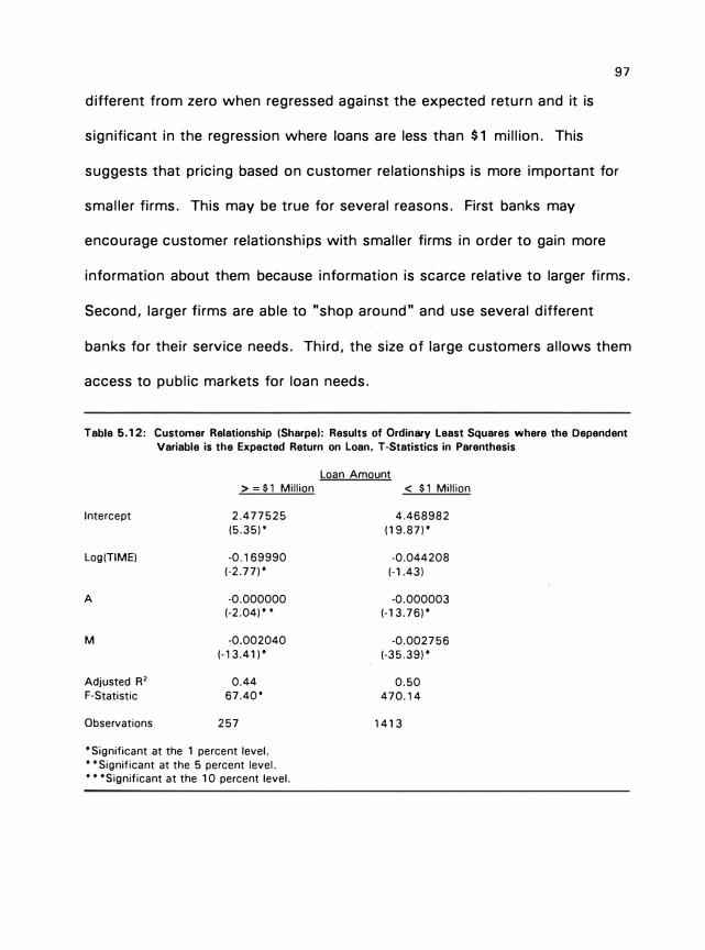
97

different from zero when regressed against the expected return and it is

significant in the regression where loans are less than $1 million. This

suggests that pricing based on customer relationships is more important for

smaller firms. This may be true for several reasons. First banks may

encourage customer relationships with smaller firms in order to gain more

information about them because information is scarce relative to larger firms.

Second, larger firms are able to "shop around" and use several different

banks for their service needs. Third, the size of large customers allows them

access to public markets for loan needs.

Table 5.12: Customer Relationship (Sharpe): Results of Ordinary Least Squares where the Dependent

Variable is the Expected Return on Loan, T-Statistics in Parenthesis

Loan Amount

> = $ 1 Million < $1 Million

Intercept 2.477525 4.468982

(5.35). (1 9.87)•

Log(TIME) -0.169990 -0.044208

(-2.77)• (-1 .43)

A -0.000000 -0.000003 (-2.04)•. (-1 3.76)•

M -0.002040 -0.002756

(-13.41)• (-35.39)•

Adjusted R2 0.44 0.50

F-Statistic 67.40. 470.14

Observations 257 1413

• Significant at the 1 percent level.

.. Significant at the 5 percent level.

• • • Significant at the 10 percent level.

CHAPTER VI

CONClUSIONS AND IMPliCATIONS

The empirical results of this study provide some rationale for the way

the case study bank prices commercial loans. Specifically, the results are

consistent with the credit rationing and customer relationship specifications

used in this study. Little support is found that commercial loans are priced

as described by the portfolio theory specification used in this study.

More generally, the empirical results of this study provide little support

that banks price commercial loans relative to risk in the strict sense

described by portfolio theory. This result is anticipated by Jaffee and Stiglitz

(1990) who argue that loan markets do not function like other markets. In

fact, the data used in this study suggest that as the riskiness of a loan

increases, the expected return to the bank decreases. This inverse

relationship provides some support for those who contend that banks price

the paper of their best customers too high and their worst customers too

low (Foss, 1992).

Some support is found for the customer relationship view that banks

offer relatively low interest rate loans to those customers whose

characteristics are expected to offer most to the long-run profits of the

bank. Consequently, when considered aside from risk, banks do grant their

98

99

best customers lower interest rates. The empirical results also provide weak

support for credit rationing which suggests that the contract interest rate on

the loan acts as a signal of credit quality, and banks ration borrowers that

exceed a certain risk level. Finally, the results of the non-nested Cox-test

suggest that the credit rationing specification used in this study provides

more explanatory power regarding the expected return on commercial loan

prices than does the customer relationship specification.

The fact that bank loans exist in illiquid markets with scarce

information provides one explanation for why this study found little support

for portfolio theory but statistically significant explanatory power in

customer relationships and credit rationing. The remainder of this chapter

uses the concept of asymmetric information to draw conclusions and

implications from the empirical results.

Illiquid Markets and Asymmetric Information

The findings described in this study are best understood when

considered within the commercial loan environment which is characterized

by illiquid assets with asymmetric information. According to Murton (1989,

p. 2 and 3),

... banks specialize in lending to a unique class of borrowers.

For these borrowers, 'public information on the economic conditions and prospects of such borrowers is so limited and expensive that the alternative of issuing marketable securities is either nonexistent or unattractive' [Goodhart, 1987, p. 86].

Because these borrowers cannot easily convey information about their own creditworthiness to lenders (or conversely, because lenders cannot easily ascertain the creditworthiness),

100

there are agency costs associated with the borrowing and

lending arrangements available to them. Banks alleviate these costs by specializing in evaluating and monitoring this class of

borrowers.

Bernanke (1983) also notes that banks are a mechanism to overcome the

information problems associated with some assets that would otherwise be

nonmarketable. Consequently, the very nature of commercial loans makes

their pricing and risk assessment very difficult.

Credit evaluation is an essential part of the process of pricing an

illiquid security, particularly because a borrower's risk classification

determines the interest rate charged which, in turn, determines the

efficiency of credit allocation in the economy. 1 Banks, however, have not

developed databases of reliable historical information about the default and

recovery rates associated with past lending. 2 Even if banks had kept good

records, Rosenberg and Kravitt ( 1993) note that it is difficult to estimate the

risk of loss on commercial loans because they are heterogeneous.

Moreover, a certain amount of subjectivity is incorporated into the loan

assessment process as various loan officers interpret the data surrounding a

prospective loan applicant.

In addition to the lack of information, the pricing of commercial loans

has intensified because of increased competition. Not only do banks face

'See, Jaffee and Modigliani ( 1 969), Jaffee and Stiglitz ( 1 990), Kao ( 1 992), and Stiglitz and Weiss (1981).

2See, for example, Morsman (1991), Larr and Stampleman (1993a and 1993b), and Rosenberg and Kravitt ( 1 993).

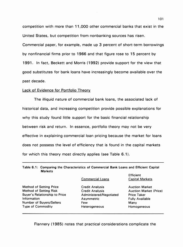
101

competition with more than 11 ,000 other commercial banks that exist in the

United States, but competition from nonbanking sources has risen.

Commercial paper, for example, made up 3 percent of short-term borrowings

by nonfinancial firms prior to 1966 and that figure rose to 1 5 percent by

1991. In fact, Beckett and Morris ( 1992) provide support for the view that

good substitutes for bank loans have increasingly become available over the

past decade.

Lack of Evidence for Portfolio Theory

The illiquid nature of commercial bank loans, the associated lack of

historical data, and increasing competition provide possible explanations for

why this study found little support for the basic financial relationship

between risk and return. In essence, portfolio theory may not be very

effective in explaining commercial loan pricing because the market for loans

does not possess the level of efficiency that is found in the capital markets

for which this theory most directly applies (see Table 6.1).

Table 6.1: Comparing the Characteristics of Commercial Bank Loans and Efficient Capital Markets

Method of Setting Price Method of Setting Risk Buyer's Relationship to Price Information

Number of Buyers/Sellers

Type of Commodity

Commercial Loans

Credit Analysis

Credit Analysis Administered/Negotiated

Asymmetric Few

Heterogeneous

Efficient

Capital Markets

Auction Market Auction Market (Price)

Price Taker

Fully Available Many

Homogeneous

Flannery (1985) notes that practical considerations complicate the

102

application of portfolio theory to bank loan selection and pricing decisions.

For example, portfolio theory assumes investors are "price takers" because

the market sets the price relative to risk and investors purchase assets at the

going price. Commercial bank loans, however, do not trade in public

markets.3 Instead, the bank examines each applicant's financial

characteristics in order to determine its creditworthiness and then

determines the contract interest rate. Moreover, Flannery notes that

portfolio models do not account for the fact that a bank's skill at analyzing

credit and its ability to bargain affects the risk-return characteristics of the

loans in its portfolio.

Credit markets also deviate from the standard models of supply and

demand because interest rates indicate what the borrower promises to repay

rather than what he will actually repay (Jaffee and Stiglitz, 1990, p. 838):

If credit markets were like standard markets, then interest rates would be the "prices" that equate the demand and supply for credit. However, an excess demand for credit is common-­applications for credit are frequently not satisfied. As a result, the demand for credit may exceed the supply at the market interest rate.

Theories of portfolio selection also assume that all relevant and

necessary information about potential investments is available. Indeed, the

availability of information is a basic assumption that leads to proper pricing.

By contrast, though, bankers work with asymmetric information. Table 5.6

31n the last few years, banks have started to securitize some commercial loans which

enables the loans to be sold more easily in public markets.

103

suggests that loans might not be priced relative to risk if the case study

bank did not adequately account for the recovery amount associated with

the loan in the case of default. Intensifying the difficulties in pricing loans

under conditions of asymmetric information is the apparent existence of an

oversupply of loanable funds which has, most likely, driven the price of

commercial loans below its associated risk level. 4

The results obtained in this study for the portfolio specification are

consistent with those stated by observers in the banking industry and thus

are probably representative of most banks. With regard to risk and pricing,

observers have found great variation in pricing practices between banks.

Three implications result from the lack of evidence for portfolio

theory. First, banks can reduce the variability of returns on their loan

portfolio by using more objective methods of measuring the individual risk of

the loan and by considering the risk of the loan relative to the entire loan

portfolio. According to Chirinko and Guill (1991, p. 19), "Ignoring

covariation [between a loan and the portfolio] would substantially understate

risk premiums." The method used in Chapter IV of this study to determine

the expected return on loans can be used by banks as a starting point to

improve their measurement of risk on loans. Other studies which suggest

similar methods include Altman (1993), Kao (1993), and Gallinger and

4See, for example, Lipen and Mitchell ( 1 993), Wall Street Journal.

104

Morgan (1993).5

Second, banks that possess more information will more accurately

assess the risk and price of loans. In this regard, information about the loan

applicant should be supplemented with economic information about the

geographic market in which the applicant operates.6 Indeed, Harrison

Young, the Federal Deposit Insurance Corporations' director of resolutions,

expects that fewer banks will be involved in commercial lending in the

future, but "The new commercial lenders will specialize either regionally or

by industry . . . " (American Banker, October 1, 1993). Moreover, Nakamura

( 1993, p. 3) argues that " ... the profitable lender is the one who best

understands the businesses that borrowers are engaged in and the value of

collateral that borrowers put up to guarantee loans."

The third implication of the portfolio theory results described in this

study is that increasing competition for commercial bank loans will continue

to pressure banks to offer interest rates that are below the risk implied by

the loan. Perhaps the force of competition, more than any other force, has

driven banks to consider loans in the broader context of the entire customer

relationship because pricing the loan in consideration of the entire

6The basic concept of portfolio management as applied to bank portfolios is presented in Larr and Stamplemen ( 1993a and 1993b).

6Ross (American Banker, October 2, 1 992) suggests that the loan portfolio should be analyzed in terms of its response to different economic events: "Industry and regional performance can be examined through simulation under a range of potential economic events, such as a significant shift in exchange rates, a Japanese financial collapse, a recession, or a pronounced regional downturn. •

105

relationship enables a bank to supplement its compensation for the risk. 7

Customer Relationships Reduce Information Problems

The results of this study also provide some support that customers

whose characteristics imply greater long-run profits for the bank are granted

lower interest rates than others. Thus, the long-run impact on profits is a

more important determinant of granting a loan than is the risk of the loan.

According to Kane and Malkiel (1965), a utility maximizing bank may agree

to grant a loan to a preferred customer even though the customer's risk will

cause the bank to experience an overall decrease in utility because not

granting the loan will also decrease utility. The implication of the customer

relationship approach is that banks can supplement low returns on loans by

other services offered by the bank such as cash management.

Customer relationships are also important to banks because they

improve the banks ability to monitor their customers. Kane and Malkiel

( 1965) argue that when a bank and customer develop a relationship through

loans or deposits, the bank is able to discern the quality of the customer.

Black (1975) and Fama (1985) also suggest that the historical relationship of

a borrower as a depositor provides the bank with information that allows it

to identify the risks of granting a loan to a particular firm and can lower the

bank's monitoring costs of that firm. Within an environment of scarce

7The desire to further compensate a bank for taking on a risky loan through the profits of additional services is likely to create tension between relationship managers and portfolio managers who may seek divergent goals.

information, the information gained about a firm through the relationship

provides the bank with the ability to more accurately price future loans.

Credit Rationing

106

Credit rationing is also an outgrowth of an illiquid market with scarce

information. Credit rationing proposes that the bank does not grant loans

beyond a certain contract interest rate because, at a ceratin point, adverse

selection and moral hazard increase the possibility that higher contract

interest rates will be associated with losses that outweigh the expected

return from the increase in interest rates. Thus, interest rates signal credit

worthiness in the absence of more reliable information. Moreover, the

relationship between the expected return and the contract rate suggests that

banks can maximize their expected return by rationing.

Credit rationing suggests that banks control risk by denying credit to

the riskiest borrowers. The internal risk rating system that most banks use

to assess the risk of commercial loans supports the credit rationing view. In

the case study bank, for example, loans are assigned a risk rating from one

through eight where one is the least risky. The bank's funds are rationed

such that firms ranked five or higher are not typically granted a loan.

The empirical tests in this study provide weak support for credit

rationing. Specifically, the results indicate that the relationship between the

contract interest rate and the expected return on the loan is positive.

107

Collateral and Pricing

Finally, this study found that the expected return associated with

collateralized loans is higher than that for loans without collateral. These

results are consistent with Boot, Thakor, and Udell (1991) who argue that

firms use collateral to obtain more favorable loan terms. In an environment

of scarce information, collateral may decrease moral hazard thereby giving

the borrower a greater incentive to repay his loans (Barro, 1976).

Further Research Questions

The results of this study suggest that further research is needed to

more fully understand commercial loan pricing. For example, even though

commercial loans are illiquid assets and exist in an environment of

asymmetric information, can they be priced relative to risk? Recently,

studies have begun to suggest ways for banks to more rigorously and

objectively access commercial loan risk. Can such measures increase the

efficiency of loan pricing? Alternatively, must loan pricing be considered an

"art" because commercial loans are too heterogenous and mathematical

tools are too general.

A tangential topic to commercial loan pricing is competition. Has the

increase in nonbank competition for loans that intensified in the 1970s and

1980s caused banks to inaccurately price loans relative to risk? Specifically,

if the least risky firms have moved to the more efficient bond markets, are

the remaining smaller and more risky firms too difficult to price because of

108

asymmetric information?

Government regulation may also play a role in explaining the results

found in this study. Did the regulation of banks prior to the 1980s

encourage inaccurate pricing of commercial loans? Is the banking industry

still undergoing a transitory period in which they are learning to more

accurately price loans because they can no longer rely on the protection of

the government from outside competition?

Finally, would actual commercial loan default probabilities improve the

results of this study with regard to portfolio theory? As noted earlier, banks

have only begun to collect default rates for commercial loans (this study

used corporate bond default rates as a proxy). When commercial loan

default rates become available, the empirical tests of this study should be

replicated.

Symbols in Text

APPENDIX A

GLOSSARY OF SYMBOLS

d; = Probability that default will occur on loan i c· = Loan customers whose relationship is valued highly by the bank E(Rb) = Bank's expected return on a loan

109

F(Rg,8) = Bank's perception of the distribution of returns on a borrower's project f(Rg,8) = Density function associated with the above i. = Contract interest rate on the loan which is set by the bank i = Time value of money equal to the nominal rate of interest or cost of funds K = Collateral L =

N =

Rg =

R; =

Rm =

VAR; =

VARP X;=

z =

8 =

(}

Initial loan amount Number of possible events Borrower's gross return on the investment Random event i Borrower's maximum rate of return on the investment Variance related to the expected return on loan i Variance on the loan portfolio Fraction of the portfolio represented by loan i The sum equal to full repayment of the loan contract (principal and

interest) Risk associated with borrower's investment project Yield on investor's project which determines whether he/she will borrow

Symbols in Regressions A; = Dollar amount of loan for loan i CORR = Correlation between the return on the bank loan portfolio and the credit

risk of the industry in which the firm belongs DEPOSITS; = Total deposits associate with borrower i DEPSTE; = Standard deviation of month-end deposits for loan i E(R;l = Expected return on loan i GROWTH; = Projected growth rate for the borrower's industry i� = Contract interest rate on loan i M; = Maturity of loan i in days RP, = Return on the bank's loan portfolio at time t TIME; = Number of days the customer has held a loan or deposits with the bank VAR; Variance of the expected return on loan i P = Regression coefficient

APPENDIX B

METHODS USED BY BANKS TO PRICE COMMERCIAL LOANS

Most financial assets are sold in markets where the forces of supply and

demand drive their risk-adjusted price toward an equilibrium. In these markets,

investors are enticed to hold risky assets by the relatively high expected returns

they offer. Because such markets do not exist for most commercial loans, bankers

must rely on their expertise and a variety of methods to price loans relative to risk.

Theory suggests that for a loan portfolio to be priced efficiently, 1 the

interest and fee income on its individual loans should incorporate 1) the bank's cost

of funds, 2 2) other costs related to the loan (such as overhead), 3) compensation

for specific risks that increase the volatility of the loan's expected returns, and 4)

compensation for portfolio risk. The bank's cost of funds normally comprises the

greatest portion of a loan's price and is easy to determine--it is equivalent to the

yield on the U.S. government security with a maturity equal to that of the loan3

1 Efficiency here means that the loan is priced exactly as it would be priced if all information were known. It is important to note that an efficiently priced loan is equivalent to its fair market price. Consequently, if a borrower were to request and obtain a lower interest rate, it would reduce the bank's expected profit. In making the decision to grant the loan, the bank would have to determine whether it could obtain a higher return if its resources were invested in an asset other than the loan. Also, an efficient portfolio is defined as the portfolio associated with the highest expected return of all portfolios available in a certain risk class, or the lowest risk of all portfolios available in a certain expected return class.

2The bank's cost of funds is comprised of the risk-free rate (government bond rate) plus the additional cost of the bank to borrow funds which is based on its own risk rating. Naturally, the cost of funds varies by bank, giving some a competitive advantage over others in their pricing of loans.

3Loans that are associated with a maturity of less than one year are generally priced relative to a shorter-term note such as the London Interbank Offered Rate (LIBOR).

110

111

plus a markup to account for the fact that loans to banks are riskier than loans to

the U.S. government. Because the four remaining components of price are more

difficult to determine, they are sometimes estimated intuitively or are not

considered at all in the commercial loan pricing process. As a result, banks often

price the loans of their best (lowest risk) customers too high and their worse

(highest risk) customers too low. In either case, though, mispriced loans lead to

the misallocation of assets in a bank's portfolio. The result is that the loan portfolio

is less than optimal in terms of expected return risk and return.

The purpose of this chapter is to review the banking literature on current and

proposed methods for pricing commercial loans. No one loan pricing model exists

that is suitable for all loans and all banks. This chapter does not attempt to

categorize loan pricing methods by bank size or customer type. Rather, it

categorizes loan pricing methods into three groups that each emphasize one aspect

of loan pricing but that must be used collectively to properly price loans. The first

method, pricing to reflect profit, provides the basis of any decision to sell a product

or a service: income and cost must be identified so that expected return can be

determined. The second method, pricing to reflect specific risks, indicates that

borrowers should be charged a premium for identifiable factors such as maturity

and industry-type that tend to increase the risk that repayment will not occur as

scheduled. The final method, pricing to reflect portfolio risk, indicates that the loan

interest rate should incorporate a premium or discount to account for the variability

an individual loan adds to or takes away from a bank's entire loan portfolio. Of the

three methods described in this chapter, pricing to reflect portfolio risk possesses

the least practical application in banking trade journals.

112

Pricing to Reflect Profitability

The first step in properly pricing loans requires that income (interest charges

and fees) and costs (direct and indirect costs associated with making, servicing,

and collecting the loan as well as an approximation of possible default) be identified

as precisely as possible so that a loan's profitability or yield can be determined.

The loan can then be accepted or rejected based on some pre-determined target

rate.

Although the identification of costs and income seems relatively straight

forward, this process can be complex. To begin the process, the bank must have

an information system with which it collects, analyzes, and makes available

relevant credit cost information to those pricing loans. The amount of information

that is needed for the pricing process depends on whether the bank's strategy

involves using relationship pricing or transaction pricing (also known as stand-alone

pricing).4

Relationship pricing is generally used by regional and community banks that

tend to service the middle-to-lower customer loan market. These banks attempt to

"cross sell" products to the customers they serve. A customer who uses the

bank's cash management services, for example, would be encouraged to borrow.

Accordingly, relationship pricing holds that customer services are interrelated and

thus loans should be priced to account for this broad relationship.5 Consequently,

4For examples, see Brick (1984), Ferrari (1992), Johnson and Grace (1990, 1991), Knight (1975), Rasmussen (1991), Rudis and Owens (1989). and Yang (1991).

6As pointed out by Ferrari (1992), stand-alone pricing should be used in conjunction with relationship pricing. He argues that banks should not devote resources to unprofitable business lines. However, accepting a small loss from one aspect of a customer relationship is wise if another facet of the relationship with the same customer is extremely profitable.

113

this approach measures the effect of such items as the compensating balances6

and cash management revenues (also called activity revenues)7 of all of the

relationships a customer possesses with the bank to determine the "loan-

relationship" profitability.

In contrast, some banks prefer to service only transaction loans.8 These

transaction (merchant) banks adhere to the stand-alone pricing perspective which

holds that customers evaluate each bank product separately and assumes that

customers may use several institutions to meet their financial needs. Thus, each

product is analyzed and priced independently of others to ensure its profitability.

Because profitability pricing provides an in-depth framework of the income

and costs that must be considered in loan pricing, two loan pricing examples are

provided. The first is based on the stand-alone view, and the second holds the

customer-relationship view.

Stand-Alone Pricing Example

The following numerical illustration from Brick (1984) shows how an

estimated yield can be determined on commercial loans by using the stand-alone

perspective. This example assumes a bank is considering a loan request for a

three-year, $1-million revolving credit (see Table B.1). The bank requires a

commitment fee of 1 /2 of 1 % per year on the unused portion of the commitment

6A compensating balance is a noninterest-bearing deposit that a commercial loan customer is required to place in the bank according to the loan agreement. Most loans do not require compensating balances, particularly upper market (large) loans.

7Cash management costs include such items as lock boxes, returned items, stop payments, and wire transfers.

6Relationship banks make transaction loans as well, but with the expectation that they will lead to a relationship.

and compensating balances of 7% of the commitment plus 5% of borrowings.

Table 8.1: Stand-Alone Loan Pricing Example

Type of loan: Commitment: Term: Contract Interest Rate: Accrual Method: Adjusted Nominal Rate·: Commitment Fee: Compensating Balances: Estimated Usage: Reserve Requirement: Options:

A. Income 1 . Interest Income

$1 Million (.75)(.0781)

2. Fee Income

Revolving credit $1 Million 3 Years 1 .1 0 x Prime (Initial Prime is 7%) Actual/360 Method 7.7% X (365/360) = 7.81%

7.70%

0.5% on Unused Portion of Commitment 7% of Commitment + 5% of Borrowings 75% (First Year) 12% Convertible into 3-year, Fixed-Rate Term Loan at

1.2 x Prime

$ 58,575

$1 Million (1-.75)(.005)

Total Income

B. Outlay 1 . Average Loan Amount

$1 Million (.75)

2. Less: Net Demand Deposit Balances $1 Million (.07) $1 Million (. 75)(.05)

Gross Demand Deposit Less: Reserve Req. @.12

Net Demand Deposits

Net Outlay

C. Estimated Loan Yield (y) y = $59,825/$655,400 = 0.0913 or 9.13%

$ 59,825

$750,000

$ 70,000

� 107,500 12.900

94.600

$655,400

114

• When the actual/365 accrual method is used, the adjusted nominal rate is the same as the contract rate.

Source: Brick (1 984).

115

The interest rate on the loan floats with the prime rate which is 7%9; and because

the borrower's default and term risk justifies a price of 1.10 times prime, the initial

contract rate on the loan is 7.7%.10 The bank uses the actual/360 accrual

method so the adjusted nominal loan rate is (365/360) x 7.8% = 7.81%. Finally,

about 75% of the commitment or $750,000 will be used during the first year of the

loan.

To estimate a loan yield (y), the bank's income must be determined net of

compensating balances and reserve requirements. Table B. 1 shows that given an

estimated first-year usage of 75% on a $1 million revolving loan, the interest and

fee amounts contribute $59,825 in total income. The outlay needed for this loan is

the average loan amount less the usable net demand deposit balances.

Consequently, the net outlay for this example loan is $655,400, which produces an

estimated yield of 9.13%. Of course, the effective yield would be higher because

9Generally the contract price of a loan is set at a fixed or variable rate and then is not reconsidered until the loan is renewed. A relatively new concept called performance based pricing, however, attempts to give the borrower an incentive to improve his/her performance (and therefore decrease his/her risk rating) by promising to decrease the contract loan rate when certain performance measures are met. More frequently, though, a schedule is attached to the loan contract that spells out increases in the contract loan rate as the credit migrates from a high quality to a lower quality loan (risk increases). If the borrower is rated by a bond rating agency such as Moody's, then the bond rating is used as the performance base by which the loan price is adjusted. In the case of non-rated firms, relevant financial ratios are used as the measure of performance.

101n this example, the riskless time value of money is incorporated into the prime rate, which is then adjusted based on the borrower's default and term risk. Using the prime rate rather than the risk-free rate as a basis for pricing the loan leads to imprecise pricing of risk because the spread between the target rate and the risk-free rate varies over time. For example, if the spread between the prime rate and the risk-free rate starts at 1 percent, then if the risk-free rate falls and the prime remains steady, the loans priced at 1 .1 times prime will be priced too high.

116

interest payments are generally made monthly or quarterly.11

The stand-alone method requires information limited to the loan itself.

Therefore, the calculations shown in Table 3.1 can be expressed in the following

simple formula12:

y = [ur + f(1-u)) I lu- (b1

+ b2u)(1-R))

where y is the estimated loan yield, u is the estimated first-year commitment usage,

r is the adjusted nominal rate, f is the commitment fee, b, is the compensating

balance requirement on the total commitment, b2 is the compensating balance

requirement on the borrowings, and A is the reserve requirement on the

compensating balances. Thus, for the example used here:

y = [(.75)(.0781) + (.005)(1-.75)) I [.75- (.07 + (.05)(.75))(1-.12)1

= .59825 I .65540 = .0913 or 9.13%.

An advantage of this pricing formula is that it allows bankers to determine

the yield on different types of commercial loans with various combinations of costs

and can be easily incorporated into a computer program. In essence, it ensures that

a loan's spread covers its costs if payments are made as scheduled. Knight (1975),

however, suggests that bank's perform more detailed analysis on their largest

customers to insure that adequate profits are generated by the entire account

relationship.

1 1The effective rate Iii is determined by the following equation: i = [ 1 + (yIn) I" - 1

where y is the estimated loan yield and n is the number of times per year interest is compounded.

121f a revolving credit or an open line uses a fixed commitment fee based on the total commitment rather than the unused portion, then the formula is y = [ur + f) I [u - (b, +

b2ull 1-AIJ.

117

Relationship Pricing

Table 8.2 shows the elements of a customer-relationship profitability

analysis as suggested by Knight. This analysis, which is typical of most, contains a

detailed listing of sources and uses of funds, income, expenses, net income, and

profitability measures.

Although the mathematics of profitability analysis are simple, the items used

to measure the relationships are difficult to determine. Moreover, one can debate

how to measure the items in this analysis. Johnson and Grace ( 1990), for

example, show that the treatment of deposit balances in a profitability analysis has

a significant impact on the loan's expected yield. The "total funds" approach gives

the customer credit for deposits and uses the total funds borrowed as the base on

which to measure profitability. The "net borrowed funds" model, however,

essentially credits customer deposits at the bank's cost of funds rate by assuming

that the borrower only uses the difference between the loan balance and the

deposit balance. As a result, the net borrowed funds approach overstates the

profitability of a loan and understates the pricing.

Summary

A disadvantage of loan profitability analysis is that it requires the collection

and analysis of a detailed set of data about loans. The strength of this analysis,

however, can far outweigh the cost. Loan profitability analysis, whether

relationship or stand-alone, indicates whether the income from a loan will cover

costs if all interest and principle payments are made as scheduled. Moreover, it

draws attention to the most profitable or unprofitable accounts and products, and

thus allows more efficient allocation of resources.

118

Table 8.2: Customer-Relationship Profitability Analysis

A. Sources and Uses of Funds

1 . Average Loan Balances: $ 2. Average Collected Balances: $

a. Investable Balance (x% reserve): $ --

3. Average Time Balance: $ --

a. Investable Balance (x% reserve): $

4. Total Loanable Funds (2a + 3a): $ --

5. Bank Funds Used by Customer (1 - 4): $ --

a. Allocated Capital (8% of 1 ): $ --

b. Funds Transferred from Pool (5 -5a): $ --

B. Income

6. Gross Interest Income on Loans: $ --

7. Earnings on Deposit (x% of 4): $ --

8. Fees Paid:

a. Service Charge Fees $ --

b. Loan Commitments $ --

c. Data Processing $ --

d. Total (8a + 8b + 8c): $

9. Total Income (6 + 7 + 8): $ --

c. Expenses

10. Activity Costs from Account Analysis: $ --

11 . Interest Accrued on Time Deposits: $ --

12. Charge for Bank Funds Used:

a. Allocated Capital (20% of 5a): $ --

b. Pool Funds (x% of 5b): $

c. Total (12a + 12b): $ --

13. Loan Handling Expenses: $

14. Cost of Fee Services: $ --

15. Data Processing: $ --

16. Total Expenses ( 1 0 + 11 + 12 + 13 + 14 + 15): $ --

D. Net Income

17. Net Income Before Taxes (9 - 16): $

E. Profitability Measures

18. Allocated Capital Index (17/5a): % --

19. Net Profits/Net Funds Used (17/5): %

20. Net Profits/Gross Amount Borrowed ( 17/1): %

21. Gross Profits/Net Funds Used [17 + 12c)/5): %

Note: Activity (cash management) costs include items such as lockbox services, coin shipments, wire transfers, stop payments, and returned items. Source: Knight (1975).

119

Articles that explain methods of pricing to reflect costs, however, provide

little information about how to price the risks of ·a loan. The next section presents

loan pricing models that concentrate on pricing risk.

Pricing to Reflect Specific Risks

Financial theory indicates that the expected return on an investment

increases as risk increases.13 A larger expected return is necessary to entice risk-

averse investors to hold an instrument whose returns have greater variability than

instruments with lower risk. When investments are traded in efficient markets

where information is accessible to all investors, the price of the investment reflects

risk. Because most bank loans are not traded in an open market and exist in an

environment of asymmetric information, market-driven measures of risk do not

exist. Consequently, bankers must gather information such as current financial

data about borrowers and relationships between industries in order to accurately

assess and price the risk of each loan. As with determining costs related to a loan,

the more accurate the information about risk, the closer to a "market" price the

loan will be priced. Also, when risk is properly priced the bank's management can

be more confident that they are holding a portfolio with the mix of risk that they

desire.

This section describes four methods that have been suggested to price the

risk of bank loans. The first, measuring the default risk of a loan, uses specific

information about a particular loan applicant to assess one aspect of risk--the

13Risk is defined by the variance of the expected return around its mean. In other words, risk can be interpreted as volatility.

120

probability that the loan will not be repaid as scheduled. The second and third

methods go beyond default risk and suggest how other risk factors such as

maturity and industry-type can be measured and incorporated into the price of the

loan. A final method discussed in this section uses bond market prices to assess

the price of risk.

Pricing Default <Credit) Risk

Default risk is the probability that a borrower will not repay his/her loan

under the terms initially agreed upon. Default risk, which is dependent on the

borrower's characteristics, is determined in isolation of other loans in the bank's

portfolio. Because many methods have been developed to measure default risk and

are thoroughly discussed in the literature, only a few methods are briefly

reviewed. 14

Financial ratio analysis provided one of the earliest measurements of

bankruptcy (and default) and remains a useful method of detecting operating and

financial stress in firms. 15 Beaver (1967), for example, found that certain financial

ratios exhibited significantly different measures when comparing healthy firms with

firms experiencing financial difficulties. Moreover, certain financial ratios

discriminated between matched samples of failed and nonfailed firms for up to five

years prior to failure. Generalizing from several studies, the most helpful ratios

14For a survey of bankruptcy and loan classification models, see Altman ( 1983) and Scott (1981).

16See, for example, Altman (1968), Beaver (1967), Dietrich and Kaplan (1982), Libby (1975), and Smith and Winakor (1935).

121

were those that measured a firm's profitability, liquidity, and solvency.16

The analysis of financial ratios has been enhanced by applying statistical

techniques such as regression and multivariate discriminant analysis which consider

interactive effects and groupings of variables. Two better known models of this

type are the Z-score model and ZETA analysis. The Z-score model incorporates

working capital/total assets, retained earnings/total assets, earnings before interest

and taxes/total assets, market value equity/book value of total liabilities, and

sales/total assets in a multivariate discriminant analysis to predict firms that are

likely to go bankrupt. A study by Altman ( 1 983) indicates that the model predicted

a sample of 33 firms with 95 percent accuracy when the financial ratios were

tested one year before bankruptcy. The accuracy of the model fell to 36 percent,

however, when the ratios were tested 5 years before bankruptcy.

ZETA analysis, produced by Altman, Haldeman, and Narayanan (1977),

improved the longer-term accuracy of the Z-score by successfully classifying 90

percent of the sample firms one year prior to bankruptcy and 70 percent of the

firms up to five years prior to bankruptcy. The ZETA model relies on the following

seven variables: return on assets (earnings before interest and taxes/total assets),

stability of earnings (normalized measure of the standard error of estimate around a

1 0-year trend in the return on assets), debt service (earnings before interest and

taxes/total interest payments), cumulative profitability (retained earnings/total

181n practice, the set of ratios used often varies by the industry being analyzed. Moreover, the information content of ratios varies over time. Currently, leverage is a critical ratio as is interest and fixed charge coverage. Robert Morris Associates publishes an Annual Statement

Studies, which summarizes the financial ratios from more than 95,000 financial statements.

The statements are collected from banks and are categorized by the company's asset size and 4-digit standard industrial code.

122

assets). liquidity (common equity/total capital),a nd size (total tangible assets).

Although the above methods classify firms only into the two categories

bankrupt and nonbankrupt, they provide meaningful insight into those variables that

provide information about default. Dietrich and Kaplan (1982) extended the

bankrupt/nonbankrupt categories by developing a model that computes a score that

classifies loans into one of four mutually exclusive risk categories by using a debt-

equity ratio, a funds-flow-to-fixed-commitments ratio, and sales trends. In addition,

Bierman and Hausman (1970) suggest a dynamic programming technique that

indicates whether to offer credit to a customer based on a set of decision rules.

After determining the risk rating or default probability of a loan, it can be

incorporated into the price of the loan.17 A useful illustration is presented by

Saunders (1987) in which he assumes a contract loan rate is determined by the

risk-free and default rate. In this case, a profitable loan contract rate would be

determined by the following formula:

i. = [(1 +r)/( 1 -dll- 1

where i. is a profitable loan contract rate, r is the risk-free nominal rate of interest,

and d is the probability of default.18 Using the formula above and assuming a

default probability of 1 percent and 2 percent, Table 8.3 indicates that the pricing is

consistent financial theory which associates higher default probabilities (risk) with

higher loan contract rates. Specifically, default risk increases as credit quality

17Miller (1991 L Loan Pricing Corporation, used the cumulative seven-year default rate of Standard & Poor's bond default statistic as a proxy for the default rate for bank loans with comparable risk.

1 8To determine the dollars that would be received for every $1 lent, the formula is simply 1 + i" = ( 1 + r)/( 1-d).

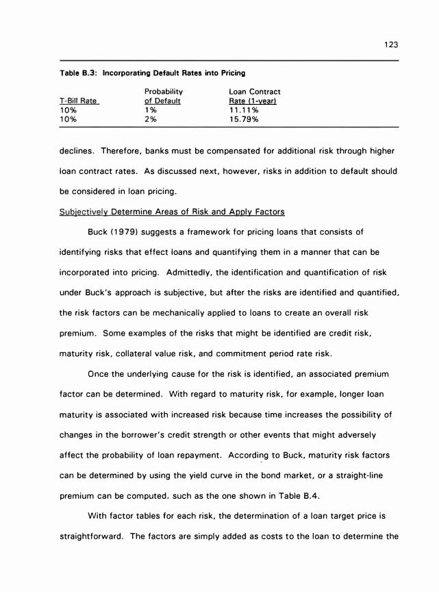
Table 8.3: Incorporating Default Rates into Pricing

T-Bill Rate

10%

10%

Probability

of Default

1%

2%

Loan Contract

Rate I 1-yearl 11.11%

15.79%

123

declines. Therefore, banks must be compensated for additional risk through higher

loan contract rates. As discussed next, however, risks in addition to default should

be considered in loan pricing.

Subjectively Determine Areas of Risk and Apply Factors

Buck (1979) suggests a framework for pricing loans that consists of

identifying risks that effect loans and quantifying them in a manner that can be

incorporated into pricing. Admittedly, the identification and quantification of risk

under Buck's approach is subjective, but after the risks are identified and quantified,

the risk factors can be mechanically applied to loans to create an overall risk

premium. Some examples of the risks that might be identified are credit risk,

maturity risk, collateral value risk, and commitment period rate risk.

Once the underlying cause for the risk is identified, an associated premium

factor can be determined. With regard to maturity risk, for example, longer loan

maturity is associated with increased risk because time increases the possibility of

changes in the borrower's credit strength or other events that might adversely

affect the probability of loan repayment. According to Buck, maturity risk factors

can be determined by using the yield curve in the bond market, or a straight-line

premium can be computed, such as the one shown in Table B.4.

With factor tables for each risk, the determination of a loan target price is

straightforward. The factors are simply added as costs to the loan to determine the

124

contract loan price. Consequently, this method prices loans relative to risk,

although the risks and associated factors are subjectively determined.

Table 8.4: Maturity Risk

Maturity Factor Maturity Factor Maturity Factor

!Yrs.) 1.%1 � 00 � 00

0-1 0 10 .94 19 1.88

2 .1 0 11 1.04 20 1.98

3 .21 12 1.15 21 2.08

4 .31 13 1.25 22 2.19

5 .42 14 1.35 23 2.29

6 .52 15 1.46 24 2.40

7 .63 16 1.56 25 2.50

8 .73 17 1.67

9 .83 18 1.77

Source: Buck ( 1 979).

A more objective approach would determine risks and associated factors by

analyzing the similarities of many loans created by many banks. Most banks do not

possess such detailed information; but as explained next, Loan Pricing Corporation

(LPC) has compiled a loan databank that has enabled them to do such analysis.

Pricing Matrix by Risk Factors

The Loan Pricing Corporation developed a pricing matrix that goes a step

beyond Buck's method by devising an objective system to determine the risk

factors and associated premiums by which to price loans. LPC developed its pricing

matrix by analyzing the similarities of over 6,000 commercial loans to borrowers

with sales over $500 million. Although much of their data were obtained from

Security and Exchange Commission filings, they also incorporated proprietary loan

data from over 45 banks nationwide.

LPC created its matrix by first using regression analysis to identify the

125

factors that explained the spread of the contract loan price from LIBOR. After

controlling for a number of variables, they found that spread pricing was

statistically significantly dependent on borrower's risk, annual sales size, and the

estimated usage level on the loan. 19 Loans were also analyzed by characteristics

such as type (secured vs. unsecured), geographic location, and industry.

Essentially, the LPC method is similar to a multifactor capital asset pricing

model where a sample of commercial loan "investments" have replaced the stock

market portfolio. As a result, the LPC matrix identifies the premiums charged by

banks for various risks and then uses these factors to identify the "market" price of

a given transaction based on comparable deals. 20

Pricing Loans Relative to Bonds

The price/risk structure created by the bond market can be a valuable

reference point to bankers in their pricing of commercial loans. Specifically,

because the bond market incorporates default risk into its return, it creates a risk

structure for interest rates.

Maniktala ( 1991 l argues that risk measures that rely on bond market data

are superior to those based on historical data for two main reasons. First, because

historical data are imbedded in a past environment, their forecasting ability is

impaired when future conditions change. In contrast, the yield of bond market data

reflects the market's estimate of future performance for a particular risk category.

19Earlier analysis by LPC indicated that commitment size also explained a significant portion of the LIBOR spread, but it was not included in their analysis because of its correlation with borrower sales.

20Banks that purchase the LPC product are given personal computer software that enable them to compute a market loan price by entering into the program characteristics of the loan such as loan purpose as well as the firm's industry type, geographic location, and asset size.

126

Moreover, bond data change daily, reflecting the incorporation of new information

about the future. Second, the availability and consistency of historical borrower-

specific data is slim because the risk-scoring systems of most banks have not been

in place for a very long period. Bond market data, on the other hand, are readily

available for long periods of time.

Maniktala suggests the following three steps to price loans relative to the

bond market. First, arrange annual corporate bond prices (available in The Wall

Street Journal) by risk and maturity. Each risk-maturity combination should

possess several bonds, while bonds with special option features should be

excluded. Second, calculate the yield to maturity for each bond and the average

yield for each risk-maturity combination. Finally, subtract the bank's cost of funds,

represented by an adjusted secondary CD rate for an equivalent maturity, from each

average yield to create the loan target. The resultant target, which shows the

average return achievable in the public debt market for corporate bonds with an

equivalent risk and maturity, can be used to determine the market-consistent return

on bank loans that possess the same risk.

Table 8.5 indicates how a bank's rating system might correlate with public

bond ratings. For institutions using a 1 0-point risk rating system, a risk rating of 1

may correspond with the bond market rating of AAA. 21 Thus, the average return

of the bank's portfolio of class 1 risks should be 0.23 percent.

2'Risk scores of 7 through 10 would be associated with bond ratings of CCC and below. Because these risk ratings represent problem credits, pricing is not a consideration.

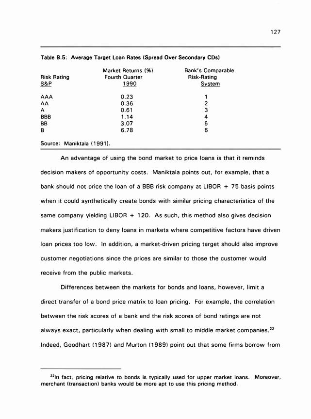
127

Table 8.5: Average Target Loan Rates (Spread Over Secondary CDsl

Market Returns (%) Bank's Comparable Risk Rating Fourth Quarter Risk-Rating

� .1JW. �

AAA 0.23 1 AA 0.36 2 A 0.61 3 888 1.14 4 88 3.07 5 8 6.78 6

Source: Maniktala (1991 ).

An advantage of using the bond market to price loans is that it reminds

decision makers of opportunity costs. Maniktala points out, for example, that a

bank should not price the loan of a 888 risk company at LI80R + 75 basis points

when it could synthetically create bonds with similar pricing characteristics of the

same company yielding LI80R + 120. As such, this method also gives decision

makers justification to deny loans in markets where competitive factors have driven

loan prices too low. In addition, a market-driven pricing target should also improve

customer negotiations since the prices are similar to those the customer would

receive from the public markets.

Differences between the markets for bonds and loans, however, limit a

direct transfer of a bond price matrix to loan pricing. For example, the correlation

between the risk scores of a bank and the risk scores of bond ratings are not

always exact, particularly when dealing with small to middle market companies. 22

Indeed, Goodhart (1987) and Murton (1989) point out that some firms borrow from

221n fact, pricing relative to bonds is typically used for upper market loans. Moreover,

merchant (transaction) banks would be more apt to use this pricing method.

128

banks because public information on their economic condition is so limited that

alternative public financing is too expensive or not available. Finally, loans tend to

possess stricter covenants but more flexibility with regard to repayment under

default while bonds possess the advantage of being more liquid.

Summary

Many different types of specific risks effect commercial bank loans.

Identifying and pricing these risks will enable a bank's loan pricing policies to more

closely approximate the true market price and more efficiently allocate available

funds. A final risk that must be considered in pricing is the general risk of loans

relative to the bank's total loan portfolio.

Portfolio Approach to Pricing

Portfolio theory indicates that loans should be priced according to their risk­

return relationship with a bank's entire loan portfolio. This theory shows that when

a loan that possesses a negatively correlated return with the bank's loan portfolio is

added to the portfolio, it reduces the overall variability of returns to the portfolio

because it acts as a hedge against movement in the rest of the portfolio. 23

Consequently, negatively correlated loans should be priced lower than loans that

are positively correlated to the portfolio, ceteris paribus.

Mersman ( 1991) noted that "Commercial loan portfolio management is in an

embryonic state in most commercial banks--contrary to what many bankers might

believe." Indeed, applying portfolio theory to commercial bank loan pricing is

difficult because it is hard to measure the risk and expected return of loans which

23This theory is explained further in Chapter Ill, op cit., under portfolio pricing theory.

129

are needed to apply the model. Given these difficulties, the literature contains little

practical application of portfolio theory to pricing commercial loans. As a result,

this section reviews only one approach: measuring risk concentrations to adjust

loan contract prices relative to its contribution to the portfolio's risk.

Diversifiable and Nondiversifiable Risk

Goodman (1981) considers the loans in a bank's portfolio to less developed

countries (LOCI that are not members of the Organization of Petroleum Exporting

Countries (OPEC). Because rate-of-return figures are not available, proxies are

developed to estimate the country risk considerations that are assumed to affect

the loan's rate of return.

The proxies chosen to estimate country risk represent possible problems that

may hinder a country's ability to repay its debts: growth in exports, money supply,

international reserves, and the ratio of imports to reserves. For each proxy, a

quarterly time series was compiled and an index for each proxy was constructed

with each country weighted by its borrowing share. A regression was performed

for each country as given by the equation:

(8.1) X;= o; + [i;'5< + e;

where ;'5<. represents the index for a given country risk measure, X; is the country

risk measure X for country i, and O; and {i; are constants. The systematic or

nondiversifiable variance for country i for a given risk measure is equal to the

squared fi; constant from the regression times the variance of the index [(.B;a)2]. The

nonsystematic or diversifiable variance is the squared standard error of the

regression times (N-2)/N where N is the number of observations.

Although this method presents an alternative to quantifying diversifiable and

130

nondiversifiable without using rate-of-return figures, it also has some drawbacks.

First, bias may be introduced if measurement errors exist in the proxies. Second,

although these measures may capture an ability to pay, they do not account for a

willingness to pay. Finally, this method can be applied to only a small number of

loans (non-OPEC LDCs) within a bank's portfolio.

Although the next article reviewed was also written with global bank lending

in mind, its application of portfolio theory possesses greater general application.

Measuring Risk Concentrations

Common underlying factors exist within every loan portfolio that cause

changes in the financial status of many borrowers. As a result, a group of loans

that react similarly to the same events can cause a bank's loan portfolio to act as if

it contained just a few large loans. For this reason, identifying covariances among

loans based on such factors as exchange rates and geographic concentration, is

important to the diversification process because it highlights sources of risk to the

portfolio. 24

Bennett (1984) uses the concept of covariance and risk concentrations to

create a method that takes into account the bank's current portfolio structure to

guide future decisions in exposure and pricing. Bennett presents this method by

using a hypothetical bank loan portfolio analyzed at the customer level.

Specifically, his method identifies the current credit rating and exposure of each

customer and then uses economic theory to consider the likely impact on customer

ratings of different events such as a $1 0 drop in oil prices, a 2% slower growth

2•1n addition, loan covariances might include interest rates, commodity prices, major local events, and particular stages of the business cycle.

, 31

rate of European countries, and a 25% depreciation of the dollar. This portion of

the analysis identifies borrowers that are sensitive to a common set of events and

thus indicates where the portfolio's risks are concentrated by showing how each

event would affect the quality of the loan portfolio. 25

The result of the event analysis can be condensed into a single portfolio risk

measure by giving specific value weights to the proportion of the portfolio in each

risk category. The value weights reflect the notion that negative events will have a

more adverse affect on the ability of weak credits to service debt than on that of

strong credits. Moreover, a portfolio risk contribution index value can be created

for each loan by considering whether the loan intensifies or mitigates the impact of

each event on the bank's entire loan portfolio. Each borrower's portfolio risk

contribution index value can then be used to guide future pricing. 26 For example,

a borrower that contributes significantly to portfolio risk should be charged a price

higher than the standard markup for its risk rating while a borrower that hedges the

portfolio risk should be priced lower than the standard markup.

Summary

The portfolio approach encourages a bank to take a broader perspective and

view individual credits in light of their affect on overall bank profitability rather than

the profit on an isolated transaction. Moreover, pricing loans based on a portfolio

approach implicitly rations credit to highly risky candidates. Specifically, if a bank

is highly concentrated in an industry with a particular earnings pattern, then

26Chirinko and Guill ( 1 991) suggest a more sophisticated method that uses macroeconomic and input/output models to estimate loan losses associated with specific events.

28The price related to the risk contribution value is added to the price which reflects its original risk rating.

additional firms with the same earnings pattern could be charged a higher loan

contract price while firms possessing opposite earnings patterns (yet the same

default rate) would be charged a lower contract rate.

132

The portfolio approach is not without its problems, however. This approach

is difficult to implement because the expected return on bank loans is difficult to

determine given the many factors that are represented in the price of a loan. Also,

like other statistical methods, a portfolio approach to pricing loans cannot fully

substitute for the informed judgement of individual lending officers or credit

analysts, but should be used in a supplemental manner.

APPENDIX C

PRESENTATION OF GENERALIZED LEAST SQUARE RESULTS

The following tables replicate the tests shown in Chapter 5, but generalized

least squares (GLS) is used rather than ordinary least squares (OLS). As noted in

Chapter 5, most of the OLS regressions tested positively for heteroscedasticity.

The data are not corrected for heteroskedasticity, however, because the nonnested

J-test and Cox-text were created for OLS regression results. In addition, parameter

estimates remain unbiased and consistent in the presence of heteroskedasticity,

even though they are inefficient. For the interested reader, however, GLS results

are shown here.

The Park-Giejser statistic, which results from these tests is not used to

weight the data. Rather, in order to use the same weighting system for all of the

models, the variables are transformed by dividing them by the amount of the loan. 1

Because the data in this chapter are transformed by the original amount of the loan,

the coefficients should be interpreted with caution. The coefficients reflect the

mean expected return per dollar amount of the loan relative to the ratio of the

independent variable in question per dollar amount of the loan.

11t is necessary to use the same weighting system for all models because the dependent variables on the competing models must be the same in order to assess the relative explanatory power of the independent variables associated with each model.

133

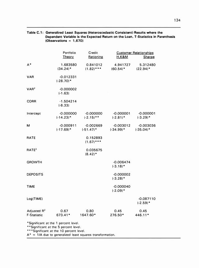
134

Table C.1: Generalized Least Squares (Heteroscedastic Consistent! Results where the

Dependent Variable is the Expected Return on the Loan, T-Statistics in Parenthesis

(Observations = 1,6701

Portfolio Credit �!.!SIQm�r R�li!IiQnl!hil2l! Theory Rationing H,K&M She me

A* 1.683580 0.841012 4.941727 5.312480

(34.241* ( 1.821 * * * (60.541* (22.941*

VAR -0.012331

(-28.701*

VAR2 -0.000002

(-1.63)

CORR -1.504214

(-8.33)

Intercept -0.000000 -0.000000 -0.000001 -0.000001

(-14.23)* (-2.15)** (-2.81 )* (-3.29)*

M -0.000911 -0.002669 -0.003012 -0.003036

(-17.69)* (-51.47)* (-34.99)* (-35.04)*

RATE 0.152893

(1.67)***

RATE2 0.035675

(8.42) *

GROWTH -0.006474

(-3.18)*

DEPOSITS -0.000002

(-3.28)*

TIME -0.000040

(-2.09)*

Log(TIME) -0.087110

(-2.59) *

Adjusted R2 0.67 0.80 0.45 0.45

F-Statistic 673.41 * 1647.60* 276.50* 446.11*

• Significant at the 1 percent level. • • Significant at the 5 percent level. • • • Significant at the 10 percent level. A • = 1 /A due to generalized least squares transformation.

135

Table C.2: Results of J-Test: Predicted Values for Re-estimated Equations, T-Statistics in Parenthesis Dependent Variable: Expected Return on Loans

H0: Credit Rationing H,: H,K&M Customer Relationship

H0: H,K&M Customer Relationship H,: Credit Rationing

• Significant at the 1 percent level. • • Significant at the 5 percent level.

Table C.3: Results of Cox Test (q Statistic)

Predicted Values for: Credit Customer Relationships Rationing H.K&M

-0.232683 (-2.10) ..

1.012713 (53.72)•

Dependent Variable: Expected Return on Loans

H0: Credit Rationing H,: H,K&M Customer Relationship

H0: H,K&M Customer Relationship H,: Credit Rationing

• Significant at the 1 percent level.

g Statistic

-1.227

-41 5.479•

Table C.4: Reconsidering the Portfolio Theory Specification Generalized Least Squares

(Heteroscedastic Consistent) Results, T-Statistics in Parenthesis (Observations =

1,670)

De(lend�nt Vari§!bl�s Ex(lect�d R�turn Premium Premium Exll�£1�!;! R�t!.lrn

A* 1.683580 1.357528 2.905803 4.852976

(34.24)* (34.11). (12.10)* (17.50)*

VAR -0.012331 0.0046077

(-28.70)* (13.25).

VAR2 0.000002 0.000011

(-1.63)* (10.05)*

RISK 0.4791333 -0.0271419

(7.77)* (-0.37)

CORA -1.504214 -1.491842 -0.0819936 -0.3929100

(-8.33) (-10.20) (-0.28) (-1.14)

Intercept -0.000000 -0.000000 -0.000001 -0.000001

(-14.23)* (-17.16)* (-3.30)* (-3.32)*

MATURITY -0.000911 0.000214 -0.000957 -0.003079

(-17.69)* (5.12)* (-13.30)* (-36.07)*

Adjusted R2 0.67 0.41 0.14 0.44

F-Statistic 673.41* 228.58* 66.61* 331.99*

• Significant at the 1 percent level. • • Significant at the 5 percent level. • • • Significant at the 1 0 percent level. A • = 1 /A due to generalized least squares transformation.

136

137

Table C.5: Portfolio Theory: Results of Generalized Least Squares (Heteroscedastic Consistent) by Loan Size where the Dependent Variable is the Expected Return on the Loan, T-Statistics in Parenthesis

Loan Size > =$1 Million < $1 Million

A• 1.605442 3.331680

(10.00)0 (44.20)0

VAR 0.001954 -0.014471

(0.62) (-37.94)0

VAR2 -0.000030 -0.000006

(-3.8W (-6.98)0

CORR -0.807830 1.434785

(-1.36) (6.43)•

Intercept -0.000000 -0.000001

(-2.59) • ( -1 2.63).

M -0.807830 -0.000976

(-1 .36) (-14.65)•

Adjusted R2 0.54 0.59

F-Statistic 59.12. 402.06°

Observations 257 1413

• Significant at the 1 percent level. • • Significant at the 5 percent level. • • • Significant at the 1 0 percent level. A • = 1 /A due to generalized least squares transformation.

138

Tabla C.6: Credit Rationing: Results of Generalized least Squares (Hataroscedastic Consistent) by

loan Size where the Dependant Variable is the Expected Return on the loan, T­

Statistics in Parenthesis

Loan Size > = $1 Million < $1 Million

A• -7.079922 1.171030

(-6.02)• (2.29)•

RATE 2.527107 0.094720

(5.99)• (0.94)

RATE2 -0.154076 0.038061

(-4.27)• (8.18)•

Intercept -0.000000 -0.000000

(1.05) (-3.66)•

M -0.003358 -0.002651

(-20.51)' (-46.93).

Adjusted R2 0.64 0.80

F-Statistic 64.40· 1405.90•

Observations 257 1413

• Significant at the 1 percent level. • • Significant at the 5 percent level. • • • Significant at the 1 0 percent level. A • = 1 /A due to generalized least squares transformation.

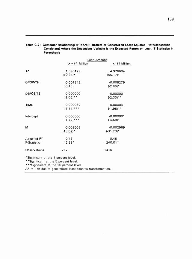
139

Table C.7: Customer Relationship (H,K&M): Results of Generalized Least Squares (Heteroscedastic

Consistent) where the Dependent Variable is the Expected Return on Loan, T-Statistics in

Parenthesis ·

Loan Amount > = $1 Million < $1 Million

A• 1.590129 4.976604

(1 0.35)• (55.17)•

GROWTH -0.001848 -0.006279

(-0.43) (-2.86)•

DEPOSITS -0.000000 -0.000001

(-2.06)•. (-2.33) ••

TIME -0.000062 -0.000041

(-1.74) .. . (-1.96) ..

Intercept -0.000000 -0.000001 (-1.72) . . . (-4.69)•

M -0.002508 -0.002969

(-13.62)• (-31.70)•

Adjusted R2 0.46 0.46

F-Statistic 42.33. 240.01.

Observations 257 1410

• Significant at the 1 percent level. • • Significant at the 5 percent level. • • • Significant at the 1 0 percent level. A • = 1/A due to generalized least squares transformation.

140

Table C.S: Customer Relationship (Sharpe): Results of Generalized Least Squares (Heteroscadastic

Consistent) where the Dependent Variable Is the Expected Return on Loan, T-Statistics In

Parenthesis

> = $1 Million

A• 3.144442 (6.15)•

Log (TIME) -0.210364 (-3.12)•

Intercept -0.000000 (-2.01 , ••

M -0.002428 (-13.49)•

Adjusted R2 0.44 F-Statistic 67.55•

Observations 257

• Significant at the 1 percent level. • • Significant at the 5 percent level. • • • Significant at the 1 0 percent level. A • = 1/A due to generalized least squares.

Loan Amount < $1 Million

5.350655 (21.40)•

-0.085661 (-2.36) ..

-0.000007 (-5.39)•

-0.002987 (-31.73)•

0.45 390.51

1413

BIBLIOGRAPHY

Akerlof, George A. !1970). "The Market for "Lemons": Quality Uncertainty and the

Market Mechanism, • Quarterly Journal of Economics 89 (August), pp. 488-500.

Altman, Edward I. !1983). Corporate Financial Distress. New York: John Wiley & Sons.

----------. !1968). "Financial Ratios, Discriminant Analysis and the Prediction of Corporate

Bankruptcy," The Journal of Finance 4 (September), pp. 589-609.

----------. !1985). "Managing the Commercial Lending Process, • in Handbook for Banking

Strategy, R.C. Aspinwall and R.A. Eisenbeis, eds. New York: Wiley, pp. 589-606.

----------. [1993a). "Valuation, Loss Reserves, and Pricing of Commercial Loans, The

Journal of Commercial Lending (August), pp. 8-25.

----------. [1992). "Valuing Loans Fairly Under FASB's Plan," American Banker, April 7, p. 4

cols. 1-4.

----------,Robert B. Avery, Robert A. Eisenbeis, and Joseph F. Sinkey, Jr. [19811.

Application of Classification Techniques in Business, Banking and Finance.

Greenwich, CT: JAI Press.

----------,Robert G. Haldeman, and P. Narayanan. [1977). "ZETA Analysis: A New Model

to Identify Bankruptcy Risk of Corporations," Journal of Banking and Finance 1

(June), pp. 29-54.

Baltensperger, Ernst. [ 1980). • Alternative Approaches to the Theory of the Banking Firm,"

Journal of Monetary Economics 6, pp. 1-37.

Barro, Robert J. [19761. "The Loan Market, Collateral and Rates of Interest. • Journal of

Money, Credit, and Banking 8 (November), pp. 439-456.

Beaver, William H. [1967). "Financial Ratios as Predictors of Failures, • Empirical Research

in Accounting: Selected Studies 1966, Journal of Accounting Research (Supplement

to Vol. 4), pp. 71-111.

Beckett, Sean and Charles Morris. [ 1 992). • Are Bank Loans Still Special? • Federal

Reserve Bank of Kansas City Economic Review (Third Quarter), pp. 71-84.

Bennett, Paul. [ 1 984). • Applying Portfolio Theory to Global Bank Lending," Journal of

Banking and Finance 8, pp. 153-169.

Berger, Allen N. and Gregory F. Udell. [1990). "Collateral, Loan Quality, and Bank Risk, •

Journal of Monetary Economics 25, pp. 21-42.

141

----------. [1989). "Some Evidence on the Empirical Significance of Credit Rationing,"

Unpublished, Board of Governors of the Federal Reserve System.

142

Berlin, Mitchell and Jan Loeys. [1988). "Bond Covenants and Delegated Monitoring, • The

Journal of Finance 43 (June), pp. 397-412.

Bernanke, Ben S. 11983). "Nonmonetary Effects of the Financial Crisis in the Propagation

of the Great Depression, • The American Economic Review (June), pp. 257-276.

Best, Ronald and Hang Zhang. [ 1992). "Alternative Information Sources and the

Information Content of Bank Loans," Presented at the Eastern Financial Meetings

(May).

Bierman, Harold, Jr. and Warren H. Hausman. 11970). "The Credit Granting Decision, •

Management Science (April), pp. 519-532.

Black, Fisher. [1975). "Bank Funds Management in an Efficient Market," Journal of

Financial Economics 2, pp. 323-339.

Blackwell, David W. and David S. Kidwell. [1988). • An Investigation of Cost Differences

Between Public and Private Placements of Debt," Journal of Financial Economics

22, pp. 253-278.

Boyd, John H. and Edward C. Prescott. [1986). "Financial Intermediary-Coalitions, •

Journal of Economic Theory 38, pp. 211-232.

Brady, Thomas F. [1985). "Changes in Loan Pricing and Business Lending at Commercial

Banks," Federal Reserve Bulletin (January), pp. 1-13.

Brennan, Michael and Alan Kraus. [1987). "Efficient Financing Under Asymmetric

Information, • The Journal of Finance 42 (December), pp. 1225-1243.

Brick, John R. [1984). "Pricing Commercial Loans, • Journal of Commercial Bank Lending

(January), pp. 44-45.

Buck, Walter H. 11979). "Risk-Management Approach to Pricing Loans and Leases,"

Journal of Commercial Bank Lending (April), pp. 2-15.

Campbell, Tim S. [1979). "Optimal Investment Financing Decisions and the Value of

Confidentiality," Journal of Financial and Quantitative Analysis 14 (December), pp.

913-924.

---------- and William S. Kracaw. [1980). "Information Production, Market Signalling and the

Theory of Financial Intermediation, • Journal of Finance 35 (September), pp. 863-

881.

Casey, Robert. [ 1 990). "Mispricing Loans," U.S. Banker (June), pp. 13-14, 56.

Chase, Sam B. Jr. [1961). "Credit Risk and Credit Rationing: Comment," Quarterly

Journal of Economics (May), pp. 319-327.

Chan, Yuk-Shee. [ 1983). "On the Positive Role of Financial Intermediation in Allocation of

143

Venture Capital in a Market with Imperfect Information," The Journal of Finance 38

(December), pp. 1543-1568.

----------and Anjan B. Thakor. [1987). "Collateral and Competitive Equilibria with Moral

Hazard and Private Information," The Journal of Finance 42 (June), pp. 345-363.

Chirinko, RobertS. and Gene D. Guill. 119911. "A Framework for Assessing Credit Risk in

Depository Institutions: Toward Regulatory Reform," Presented at New York

University Salomon Center's Conference on Deposit Insurance Reform (May 17).

Christy, George C. [ 1986). "Loan Portfolio Management: An Aggressive Approach."

Journal of Commercial Bank Lending (October). pp. 16-24.

Cox, D. R. [19611. "Tests of Separate Families of Hypothesis." in Proceedings of the

Fourth Berkeley Symposium on Mathematical Statistics and Probability, Vol. 1.

Berkeley: University of California Press, pp. 105-123.

----------. [19621. "Further Results on Tests of Separate Families of Hypotheses," Journal

of the Royal Statistical Society, Series B 24, pp. 406-424.

Davidson, R. and J. MacKinnon. 11981]. "Several Tests for Model Specification in the

Presence of Alternative Hypotheses." Econometrica 49, pp. 781-793.

Deakin, Edward B. I 19721. "A Discriminant Analysis of Predictors of Business Failure."

Journal of Accounting Research Reports (March). pp. 167-179.

De Vany, ArthurS. [19851. "Comment on Modeling the Banking Firm: A Survey." Journal

of Money, Credit, and Banking 16 (November). pp. 603-609.

Diamond, Douglas W. [1984). "Financial Intermediation and Delegated Monitoring,·

Review of Economic Studies 51 (July). pp. 393-414.

----------and Philip H. Dybvig. [1983]. "Bank Runs, Deposit Insurance, and Liquidity."

Journal of Political Economy 91 , pp. 401 -41 9.

Dietrich, J. Richard. 11984). "Discussion of Methodological Issues Related to the

Estimation of Financial Distress Prediction Models," Journal of Accounting Research

22 (Supplement), pp. 83-85.

Dutta, M. [1975). Econometric Methods. Cincinnati: South -Western Publishing Company.

Eaton, J. and M. Gersovitz. [1981]. "Debt with Potential Repudiation: Theoretical and

Empirical Analysis," Review of Economic Studies, pp. 289-309.

Eisenbeis, Robert A. [1987). Discussion of "Credit Granting: A Comparative Analysis of

Classification Procedures." The Journal of Finance 42 (July). pp. 681-683.

Elton, Edwin J. and Martin J. Gruber. [1987). Modern Portfolio Theory and Investment

Analysis. New York: John Wiley & Sons.

Evans, David S. and Boyan Jovanovic. [1989]. "An Estimated Model of Entrepreneurial

Choice under Liquidity Constraints." Journal of Political Economy 97, pp. 808-827.

Fair, Ray C. and Dwight M. Jaffee. 11970). "Methods of Estimation for Markets in

Disequilibrium," Econometrica.

Fama, Eugene F. [1970). "Efficient Capital Markets: A Review of Theory and Empirical

Work," The Journal of Finance (May), pp. 383-417.

144

----------. [19851. "What's Different About Banks?" Journal of Monetary Economics 15, pp.

29-39.

----------and J. MacBeth. [19731. "Risk, Return and Equilibrium: Empirical Test," Journal

of Political Economy (May -June), pp. 607-635.

Ferrari, Richard H. [19921. "Commercial Loan Pricing and Profitability Analysis, Part I,"

The Journal Commercial Lending (February), pp. 49-59.

Fisher, Lawrence. [1959). "Determinants of Risk Premiums on Corporate Bonds," The

Journal of Political Economy, pp. 217-237.

Fissel, Gary S. and Tullio Jappelli. [1990). "Do Liquidity Constraints Vary over Time?

Evidence From Survey and Panel Data," Journal of Money, Credit, and Banking 22

(May), pp. 253-262.

Flannery, Mark J. [1985). "A Portfolio View of Loan Selection and Pricing," in Handbook

for Banking Strategy, R. C. Aspinwall and R. A. Eisenbeis, eds. New York: John

Wiley & Sons, pp. 457-472.

Foss, Greg. [1992). "Capital Allocation and Pricing Credit Risk," Journal of Commercial

Lending (October), pp. 35-44.

Freimer, Marshall and Myron J. Gordon. [1965). "Why Bankers Ration Credit," Quarterly

Journal of Economics 79 (August), pp. 397-416.

Frydman, Halina, Edward I. Altman, and Duen-Li Kao. [1985). "Introducing Recursive

Partitioning for Financial Classification: The Case of Financial Distress," The Journal

of Finance (March), pp. 269-291.

Goldfeld, Stephen M. [1985). "Comment on Modeling the Banking Firm: A Survey,"

Journal of Money, Credit, and Banking 16 (November), pp. 609-611.

Gollinger, Terri L. and John B. Morgan. [1993). "Calculation of an Efficient Frontier for a

Commercial Loan Portfolio," Journal of Portfolio Management 2 (Winter), pp. 39-46.

Goodman, Laurie S. [1981). "Bank Lending to Non-OPEC LDC's: Are Risks Diversifiable?"

Federal Reserve Bank of New York Quarterly Review, Summer, pp. 10-20.

Gorton, Gary and George Pennacchi. [1990). "Financial Intermediaries and Liquidity

Creation," The Journal of Finance 45 (March), pp. 49-71 .

Greene, William H. [1993). Econometric Analysis Second Edition. New York: Macmillan

Publishing Company.

Guttentag, Jack and Richard Herring. [1984). ".Credit Rationing and Financial Disorder,"

145

The Journal of Finance (December), pp. 1359-1389.

Harris, Milton and Arthur Raviv. [ 1 990]. • Capital Structure and the Informational Role of

Debt, • The Journal of Finance 45 (June), pp. 321-349.

Harrison, William B. and Paul A. Meyer. [1975]. "Banks' Buffer Accounts, Uncertainty, and Institutional Variables, • Southern Economic Journal, pp. 107-119.

Hart, Oliver D. and Dwight M. Jaffee. [1974). "On the Application of Portfolio Theory to Depository Financial Intermediaries, • Review of Economic Studies (January), pp. 129-147.

Hester, Donald D. and James L. Pierce. [1975]. Bank Management and Portfolio Behavior.

New Haven: Yale University Press.

----------. [1979]. "Customer Relationships and Terms of Loans: Evidence from a Pilot

Survey," Journal of Money, Credit, and Banking 11 (August), pp. 349 -35 7.

----------. [1962]. "An Empirical Examination of a Commercial Bank Loan Offer Function,"

Yale Economic Essays 2, pp. 3-57.

Hodgman, Donald R. [1963). Commercial Bank Loan and Investment Policy. Champaign, IL.: University of Illinois, Bureau of Economic and Business Research.

--------- -. [1960]. "Credit Risk and Credit Rationing," Quarterly Journal of Economics 74 (May), pp. 258-278.

----------. [1961]. "Credit Risk and Credit Rationing: A Reply," Quarterly Journal of

Economics 75 (May), pp. 327 -329.

----------. [1961 b ]. "The Deposit Relationship and Commercial Bank Investment Behavior,"

The Review of Economics and Statistics (August), pp. 257-268.

Jaffee, Dwight M. [1971]. Credit Rationing and the Commercial Loan Market. New York:

John Wiley & Sons.

---------- and Franco Modigliani. [ 19691. "A Theory and Test of Credit Rationing," The

American Economic Review 59 (December), pp. 850-872.

--------- -and Thomas Russell. [1976]. "Imperfect Information, Uncertainty, and Credit

Rationing," Quarterly Journal of Economics 90 (November), pp. 651-666.

----------and Joseph Stiglitz. [1990). "Credit Rationing," in Handbook of Monetary

Economics, Vol. 2, Benjamin M. Friedman and Frank H. Hahn, eds. New York:

North - Holland, pp. 838 -888.

James, Christopher. [1987). "Some Evidence on the Uniqueness of Bank Loans," Journal

of Financial Economics 19 (December), pp. 217-235.

Johnson, Richard D. and Jack 0. Grace. [1991). "Can Lenders Rely on Expected Loan

Yields?" The Bankers Magazine (May/June), pp. 59-66.

----------. [1990). •The Impact of Deposit Balances on Loan Pricing and Profitability

Analysis, • The Journal of Commercial Bank Lending (September), pp. 31-39.

Johnston, J. [1972). Econometric Methods Second Edition. New York: McGraw-Hill

Book Company.

Kane, Edward J., and Burton G. Malkiel. [1965]. ·sank Portfolio Allocation, Deposit

Variability, and the Availability Doctrine, • Quarterly Journal of Economics 79

(February), pp. 113-134.

Kao, Duen-Li. [1993]. •Illiquid Securities: Issues of Pricing and Performance

Measurement, • in Fixed Income Management: Issues and Solutions. New York:

Irwin.

----------. [1992). •valuation Approaches Under FASB No. 107, • Balance Sheet

Magazine (December).

146

Keeton, William R., and Charles S. Morris. [1987). ·why Do Banks' Loan Losses Differ,"

Federal Reserve Bank of Kansas City Economic Review (May), pp. 3-21.

Kim, Moshe and Vojislav Maksimovic. [1990). "Debt and Input Misallocation," The Journal

of Finance 45 (July), pp. 795-81 6.

Knight, Robert E. 119751. "Customer Profitability Analysis," Federal Reserve Bank of

Kansas City Monthly Review (April), pp. 11-20.

Lang, William W. and Leonard I. Nakamura. [1989). •Information Losses in a Dynamic

Model of Credit," The Journal of Finance 44 (July), pp. 731-746.

Larr, Peter and Arthur Stampleman. [1993a). "Concepts of Portfolio Management Part 1: Measuring and Controlling Risk," The Journal of Commercial Lending (June), pp. 6-

11 .

----------. [ 1993b). "Concepts of Portfolio Management Part 2: Understanding and Using

the Model," The Journal of Commercial Lending (August), pp. 26-31 .

Leland, Haynes and David Pyle. [1977). "Information Asymmetries, Financial Structure

and Financial Intermediation," The Journal of Finance 32 (May), pp. 371-387.

Libby, Robert E. [ 1975). "Accounting Ratios and the Prediction of Failure: Some

Behavioral Evidence," Journal of Accounting Research (Spring), pp. 150-161.

Lipin, Steven and Constance Mitchell. [1993]. "Wall Street Is Using Junk Bonds to Take

Another Slice of Banks' Lending Pie, • The Wall Street Journal, p. C1, cols. 2-4 and

p. C20, cols. 4-6.

Loomis, Floyd A. [1993). •The Coming Boom in Loan Demand and the Need for Loan Loss

Information," The Weekly Loan Pricing Report Gold Sheets (May 17, 1993), pp. 1,

18, and 20.

----------. [1991 a). "Performance-Based Loan Pricing Techniques," Journal of

Commercial Bank Lending (October), pp. 7-17.

147

----------. [1991 b). "Performance Pricing Increases and Diversification," Loan Pricing Report

(July), pp. 6-14.

Lummer, Scott L. and John J. McConnell. [19891. "Further Evidence on the Bank Lending

Process and the Capital-Market Response to Bank Loan Agreements," Journal of

Financial Economics 25, pp. 99-122.

Maniktala, Anand. [1991]. "Pricing of Risk by Banks," The Journal of Commercial Bank

Lending (December), pp. 27-32.

Marais, M. Laurentius, James M. Pattell, and Mark A. Wolfson. [1984). "The Experimental

Design of Classification Models: An Application of Recursive Partitioning and

Bootstrapping to Commercial Bank Loan Classification," Journal of Accounting

Research (Vol. 22 Supplement 1984), pp. 87-114.

Markowitz, Harry. !19521. "Portfolio Selection," Journal of Finance 7 (March), pp. 77-91.

McManus, Doug. [1992). "Diversification and Risk in Banking: Evidence from Ex Post

Returns," Presented at a Finance Seminar at the University of North Carolina at

Chapel Hill, March 13.

McNamara, Mary E. and Gita M. Srinivasan. !1992). "Loan Pricing Matrix," Technical

Paper 01-92.

Melnik, Arie and Steven E. Plaut. !19861. "The Economics of Loan Commitment

Contracts: Credit Pricing and Utilization," Journal of Banking and Finance 10, pp.

267-280.

Mehta, Dileep. [ 19681. "The Formulation of Credit Policy Models," Management Science

22 (October), pp. B30-B50.

Milde, Hellmuth and John G. Riley. [ 1 988). "Signalling in Credit Markets," Quarterly

Journal of Economics (February), pp. 101-129.

Miller, Merton H. !1962). Further Comment of "Credit Risk and Credit Rationing,"

Quarterly Journal of Economics 76 (August), pp. 480-493.

Miller, Steven C. !1991 a). "A Benchmark for Loan Loss Allocation," Loan Investor

Services Research Brief, Vol. II, No. 9A (September).

----------. [1991 b). "Mapping Out an Efficient Frontier--Risk/Return of Bank Loans vs.

Unsecured Bonds," Loan Investor Services Research Brief 1 (New York: Loan

Pricing Corporation).

Mersman, Edgar M., Jr. !1991). "Returning Commercial Lending to Profitability," The

Bankers Magazine (July/August), pp. 21-26.

Murphy, Neil B. [1968). "A Cross-Section Analysis of Demand Deposit Variability,"

Journal of Financial Quantitative Analysis (March), pp. 87-95.

----------. [1969). "A Study of Wholesale Banking Behavior." Research Report of the

Federal Reserve Bank of Boston, No. 44.

148

Murton, Arthur J. [1989). w Bank Intermediation, Bank Runs, and Deposit Insurance/ FDIC

Banking Review (Spring/Summer), pp. 1-1 0.

Myers, Stewart C. and Nicholas S. Majluf. [1984). w corporate Financing and Investment

Decisions When Firms have Information that Investors do not Have, w The Journal of

Financial Economics 13, pp. 187-221.

Nakamura, Leonard I. [1993). w lnformation Externalities: Why Lending May Sometimes

Need a Jump Start, w Federal Reserve Bank of Philadelphia Business Review

(January/February), pp. 3-14.

Olsen, Chris. [1984). w Discussion of The Experimental Design of Classification Models:

An Application of Recursive Partitioning and Bootstrapping to Commercial Bank

Loan Classifications, Journal of Accounting Research 22 (Supplement), pp. 11 5-

118.

Orgler, Y.E. [1975). Analytical Methods in Loan Evaluation. Lexington, MA.: Lexington

Books.

Pesaran, M. Hashem. [19871. "Non-Nested Hypotheses," in The New Palgrave A

Dictionary of Economics, John Eatwell, Murray Milgate, and Peter Newman, eds.

London: The MacMillan Press Limited.

----------. [ 1974). "On the General Problem of Model Selection," Review of Economic

Studies 41, pp. 153-171.

Pennacchi, George G. [19881. "Loan Sales and the Cost of Bank Capital," The Journal of

Finance 43 (June), pp. 375-396.

Rasmussen, Claus. [1991). "A Danish View on Loan Pricing," The Bankers Magazine

(November/December), pp. 42-47

Rehm, Barbara A. [1993). "Bleak Future Seen for Commercial Lending," American Banker,

1 October, p. 3, eels. 1-4.

Rickmeier, John E. [19911. "Loan Pricing: Use Risk-Adjusted Return to Price Profitably,"

Commercial Lending Review (Fall), pp. 80-83.

Robert Morris Associates. [19831. Computerized Credit Analysis. Philadelphia, PA: Robert

Morris Associates.

----------. [1986). Credit Considerations: Financial and Credit Characteristics of Selected

Industries. Philadelphia, PA.

Rose, Sanford. [1992). "Banks Neglect Use of Models in Loan Analysis," American Banker

28 January, p. 1, col. 1 and p. 8, eels. 1-5.

----------. [1992). "What's Ahead for Wholesale Intermediation," American Banker, 22 June

p. 1, col. 1, and pp. 7-10, 14-15, eels. 1-5.

149

Rosenberg, Richard and Jason Kravitt. [ 1993]. "How Feasible Is the Securitization of Loans to Small and Medium-sized Businesses?" Commercial Lending Review 8 (Fall),

pp. 4-21.

Ross, Paul. [1992]. "Is Your Loan Portfolio Really Diversified?" American Banker, 2

October, p. 4, cols. 1-4 and p. 6, cols. 1-2.

Rothschild, Michael and Joseph E. Stiglitz. [1971]. "Increasing Risk: I. A Definition, •

Journal of Economic Theory 2, pp. 225-243.

Rudis, David and John Owens. [ 1989]. • Account Profitability Hones Marketing, Improves

Pricing, • Commercial Lending Review (Summer), pp. 35-41.

Ryder, Carl E. Jr. [ 1962]. "'Credit Risk and Credit Rationing:' Comment, • Quarterly

Journal of Economics 76 (August), pp. 471-479.

Santomero, Anthony M. [1985]. "Modeling the Banking Firm, • Journal of Money, Credit,

and Banking 16 (November). pp. 576-616.

----------. [1985]. "Pricing Business Credit," in Handbook for Banking Strategy, R.C.

Aspinwall and R.A. Eisenbeis, eds. New York: Wiley, pp. 589-606.

Saunders, Anthony. [1987]. "The Interbank Market, Contagion Effects, and International

Financial Crises," in Threats to International Financial Stability, Richard Portes and

Alexander K. Swoboda, eds. Cambridge: Cambridge University Press.

Schreft, Stacey L. and Anne P. Villamil. [ 1 992]. "Credit Rationing by Loan Size in

Commercial Markets," Federal Reserve Bank of Richmond Economic Review 78

(May/June). pp. 3-8.

Scott, Ira 0. [1957]. "The Availability Doctrine: Theoretical Underpinnings," Review of

Economic Studies (October). pp. 41-48.

Scott, James. [1981]. "The Probability of Bankruptcy, A Comparison of Empirical

Predictions and Theoretical Models," Journal of Banking and Finance 5, pp. 317-

344.

Seward, James K. [1990]. "Corporate Financial Policy and the Theory of Financial

Intermediation," The Journal of Finance 45 (June), pp. 351-377.

Sharpe, Steven A. [1990]. "Asymmetric Information, Bank Lending, and Implicit

Contracts: A Stylized Model of Customer Relationships," The Journal of Finance

45 (September), pp. 1 069-1 087.

Silber, William L. and Murray E. Polakoff. [1970]. "The Differential Effects of Tight

Money; An Econometric Study," The Journal of Finance (March). pp. 83-97.

Sinkey, Joseph F., Jr. [1989]. Commercial Bank Financial Management, Third Edition.

New York: Macmillan Publishing Company.

Slovin, Myron B. and Marie Elizabeth Sushka. [ 1983]. "A Model of the Commercial Loan

Rate," The Journal of Finance 38 (December). pp. 1583-1596.

Smith, Paul F. 11978]. Money and Financial Intermediation. New Jersey: Prentice-Hall,

Inc.

150

Srinivasan, Venkat and Yong H. Kim. [1987). "Credit Granting: A Comparative Analysis

of Classification Procedures," The Journal of Finance 42 (July), pp. 665-681.

Srinivasan, Gita and Mary McNamara. [1991). "Matrix Pricing--Using Market Knowledge to

Gain a Competitive Edge, • New York: Loan Pricing Report.

Standard & Poor's. [1991]. "Corporate Bond Default Study, • Creditweek, 16 September,

pp. 1-5.

----------. [1993]. "Corporate Default, Rating Transition Study Updated, • Creditweek,

25 January, pp. 1-12.

----------. [1992]. "Study Examines Recovery Rate of Defaulted Bonds," Creditweek, 20

July, pp. 43-44.

Stigler, George J. [1976]. "Imperfections in the Capital Market, • Journal of Political

Economy 85 (June}, pp. 287-292.

Stiglitz, J. E., and A. Weiss. 11981). "Credit Rationing in Markets with Imperfect

Information, • American Economic Review (June}, pp. 393-409.

----------. [ 1986]. "Credit Rationing and Collateral, • in Recent Developments in Corporate

Finance, Jeremy Edwards, Julian Franks, Colin Mayer, and Stephen Schaefer, eds.

Cambridge: Cambridge University Press.

----------. [1987]. "Credit Rationing: Reply," The American Economic Review 77 (March},

pp. 228-231.

Strong, John S. [ 1989]. "The Market Valuation of Credit Market Debt, • Journal of Money,

Credit, and Banking 21 (August}, pp. 307-320.

Taggart, Robert A. Jr. 11985]. "Comment on Modeling the Banking Firm: A Survey,"

Journal of Money, Credit, and Banking 16 (November}, pp. 612-616.

Tobin, James. [ 1958]. "Liquidity Preference as Behavior Toward Risk," Review of

Economic Studies 25 (February), pp. 65-86.

U.S. Department of Commerce. [1990]. Regional Projections to 2040, Volume 1.

Washington D.C.: Government Printing Office.

U.S. Department of Labor. [1992]. Outlook: 1990-2005. Washington D.C.: Government

Printing Office.

Walter, lngo. [1981). "Country Risk, Portfolio Decisions and Regulation in International

Bank Lending, • Journal of Banking and Finance 5 (March}, pp. 77-92.

Yancey, T. A., G. G. Judge, and M. E. Bock. [1981 J. "Testing Multiple Equality and

Inequality Hypothesis in Economics," Economic Letters 7, pp. 249-255.

151

Yang, Gilber Y. [19911. "Pricing for Profit," The Bankers Magazine (September/October),

pp. 53-59.

Yawitz, Jess B., George H. Hempel, and William J. Marshall. [1975]. "The Use of Average

Maturity as a Risk Proxy in Investment Portfolios." The Journal of Finance (May}.

pp. 325-340.

Zmijewski, Mark E. [1984]. "Methodological Issues Related to the Estimation of Financial

Distress Prediction Models," Journal of Accounting Research 22 (Supplement}.

pp. 59-82.

VITA