An Investigation into Wave Run-up on Vertical Surface ...
196
An Investigation into Wave Run-up on Vertical Surface Piercing Cylinders in Monochromatic Waves A Thesis submitted in Fulfilment of the Requirements for the Degree of Doctor of Philosophy by Michael Morris-Thomas School of Oil and Gas Engineering Faculty of Engineering, Computing and Mathematics 2003
Transcript of An Investigation into Wave Run-up on Vertical Surface ...

An Investigation into Wave Run-up on Vertical
Surface Piercing Cylinders in Monochromatic
Waves
A Thesis submitted in Fulfilment of the Requirements for the
Degree of Doctor of Philosophy
by
Michael Morris-Thomas
School of Oil and Gas Engineering
Faculty of Engineering, Computing and Mathematics
2003


Abstract
Wave run-up is the vertical uprush of water when an incident wave impinges on a free-surface penetrating body. For large volume offshore structures the wave run-up on theweather side of the supporting columns is particularly important for air-gap design andultimately the avoidance of pressure impulse loads on the underside of the deck structure.This investigation focuses on the limitations of conventional wave diffraction theory, wherethe free-surface boundary condition is treated by a Stokes expansion, in predicting theharmonic components of the wave run-up, and the presentation of a simplified procedurefor the prediction of wave run-up. The wave run-up is studied on fixed vertical cylindersin plane progressive waves. These progressive waves are of a form suitable for descriptionby Stokes’ wave theory whereby the typical energy content of a wave train consists of onefundamental harmonic and corresponding phase locked Fourier components. The choiceof monochromatic waves is indicative of ocean environments for large volume structures inthe diffraction regime where the assumption of potential flow theory is applicable, or moreformally A/a < O(1) (A and a being the wave amplitude and cylinder radius respectively).One of the unique aspects of this work is the investigation of column geometry effects - interms of square cylinders with rounded edges - on the wave run-up. The rounded edges ofeach cylinder are described by the dimensionless parameter rc/a which denotes the ratio ofedge corner radius to half-width of a typical column with longitudinal axis perpendicularto the quiescent free-surface.
An experimental campaign was undertaken where the wave run-up on a fixed columnin plane progressive waves was measured with wire probes located close to the cylinder.Based on an appropriate dimensional analysis, the wave environment was represented bya parametric variation of the scattering parameter ka and wave steepness kA (where k
denotes the wave number). The effect of column geometry was investigated by varyingthe edge corner radius ratio within the domain 0 ≤ rc/a ≤ 1, where the upper and lowerbounds correspond to a circular and square shaped cylinder respectively. The water depthis assumed infinite so that the wave run-up caused purely by wave-structure interaction isexamined without the additional influence of a non-decaying horizontal fluid velocity andfinite depth effects on wave dispersion.
The zero-, first-, second- and third-harmonics of the wave run-up are examined todetermine the importance of each with regard to local wave diffraction and incident wavenon-linearities. The modulus and phase of these harmonics are compared to correspond-ing theoretical predictions from conventional diffraction theory to second-order in wavesteepness. As a result, a basis is formed for the applicability of a Stokes expansion to thefree-surface boundary condition of the diffraction problem, and its limitations in terms oflocal wave scattering and incident wave non-linearities.
An analytical approach is pursued and solved in the long wavelength regime for the in-teraction of a plane progressive wave with a circular cylinder in an ideal fluid. The classicalStokesian assumption of infinitesimal wave amplitude is invoked to treat the free-surface
i

boundary condition along with an unconventional requirement that the cylinder width isassumed much smaller than the incident wavelength. This additional assumption is jus-tified because critical wavelengths for wave run-up on a fixed cylinder are typically muchlarger in magnitude than the cylinder’s width. In the solution, two coupled perturbationschemes, incorporating a classical Stokes expansion and cylinder slenderness expansion,are invoked and the boundary value problem solved to third-order. The formulation ofthe diffraction problem in this manner allows for third-harmonic diffraction effects andhigher-order effects operating at the first-harmonic to be found.
In general, the complete wave run-up is not well accounted for by a second-order Stokesexpansion of the free-surface boundary condition and wave elevation. This is however,dependent upon the coupling of ka and kA. In particular, whilst the modulus and phaseof the second-harmonic are moderately predicted, the mean set-up is not well predictedby a second-order Stokes expansion scheme. This is thought to be caused by higherthan second-order non-linear effects since experimental evidence has revealed higher-orderdiffraction effects operating at the first-harmonic in waves of moderate to large steepnesswhen ka ¿ 1.
These higher-order effects, operating at the first-harmonic, can be partially accountedfor by the proposed long wavelength formulation. For small ka and large kA, subsequentcomparisons with measured results do indeed provide a better agreement than the classicallinear diffraction solution of Havelock (1940). To account for the complete wave run-up,a unique approach has been adopted where a correction is applied to a first-harmonicanalytical solution. The remaining non-linear portion is accounted for by two methods.The first method is based on regression analysis in terms of ka and kA and providesan additive correction to the first-harmonic solution. The second method involves anamplification correction of the first-harmonic. This utilises Bernoulli’s equation appliedat the mean free-surface position where the constant of proportionality is empiricallydetermined and is inversely proportional to ka.
The experimental and numerical results suggest that the wave run-up increases asrc/a → 0, however this is most significant for short waves and long waves of large steep-ness. Of the harmonic components, experimental evidence suggests that the effect of avariation in rc/a on the wave run-up is particularly significant for the first-harmonic only.Furthermore, the corner radius effect on the first-harmonic wave run-up is well predictedby numerical calculations using the boundary element method. Given this, the proposedsimplified wave run-up model includes an additional geometry correction which accountsfor rc/a to first-order in local wave diffraction.
From a practical view point, it is the simplified model that is most useful for platformdesigners to predict the wave run-up on a surface piercing column. It is computationallyinexpensive and the comparison of this model with measured results has proved morepromising than previously proposed schemes.
ii

Contents
Abstract i
Acknowledgements vii
Nomenclature ix
1 Introduction 1
1.1 Motivation . . . . . . . . . . . . . . . . . . . . . . . . . . . . . . . . . . . . 21.2 Historical Content . . . . . . . . . . . . . . . . . . . . . . . . . . . . . . . . 41.3 Thesis Statement and Outline . . . . . . . . . . . . . . . . . . . . . . . . . . 8
2 Experimental Campaign 10
2.1 Dimensionless Parameters . . . . . . . . . . . . . . . . . . . . . . . . . . . . 102.2 A Review of the Literature . . . . . . . . . . . . . . . . . . . . . . . . . . . 122.3 Experimental Procedure . . . . . . . . . . . . . . . . . . . . . . . . . . . . . 15
2.3.1 Model Configuration . . . . . . . . . . . . . . . . . . . . . . . . . . . 162.3.2 Instrumentation and Measurement . . . . . . . . . . . . . . . . . . . 182.3.3 The Wave Environment . . . . . . . . . . . . . . . . . . . . . . . . . 19
2.4 Data Analysis Methods . . . . . . . . . . . . . . . . . . . . . . . . . . . . . 202.4.1 Discrete Fourier Transform . . . . . . . . . . . . . . . . . . . . . . . 202.4.2 The Actual Wave Run-up . . . . . . . . . . . . . . . . . . . . . . . . 21
2.5 Preliminary Discussions of the Experimental Results . . . . . . . . . . . . . 232.5.1 Theoretical Considerations . . . . . . . . . . . . . . . . . . . . . . . 232.5.2 Contamination from Free Waves . . . . . . . . . . . . . . . . . . . . 252.5.3 Relative Harmonic Contributions . . . . . . . . . . . . . . . . . . . . 272.5.4 Edge Waves . . . . . . . . . . . . . . . . . . . . . . . . . . . . . . . . 29
2.6 Chapter Summary . . . . . . . . . . . . . . . . . . . . . . . . . . . . . . . . 31
3 Wave Run-up on a Circular Cylinder 32
3.1 The Boundary Value Problem . . . . . . . . . . . . . . . . . . . . . . . . . . 333.1.1 Stokes’ Expansion . . . . . . . . . . . . . . . . . . . . . . . . . . . . 34
3.2 An Infinitely Long Vertical Wall . . . . . . . . . . . . . . . . . . . . . . . . 363.3 First-Order Solution for a Circular Cylinder . . . . . . . . . . . . . . . . . . 37
iii

3.4 Second-Order Diffraction Analysis . . . . . . . . . . . . . . . . . . . . . . . 393.4.1 Convergence Studies of the Numerical Results . . . . . . . . . . . . . 423.4.2 Second-Order Numerical Results . . . . . . . . . . . . . . . . . . . . 44
3.5 Some Simplified Methods . . . . . . . . . . . . . . . . . . . . . . . . . . . . 463.5.1 Correction Factor Method . . . . . . . . . . . . . . . . . . . . . . . . 463.5.2 Velocity Head Method . . . . . . . . . . . . . . . . . . . . . . . . . . 473.5.3 Superposition Method . . . . . . . . . . . . . . . . . . . . . . . . . . 47
3.6 Experiments and Theory Compared . . . . . . . . . . . . . . . . . . . . . . 483.6.1 The Actual Wave Run-up . . . . . . . . . . . . . . . . . . . . . . . . 483.6.2 Harmonic Components and Theory Compared . . . . . . . . . . . . 513.6.3 Regression Analysis . . . . . . . . . . . . . . . . . . . . . . . . . . . 66
3.7 Some Comments on Discrepancies . . . . . . . . . . . . . . . . . . . . . . . 673.8 Chapter Summary . . . . . . . . . . . . . . . . . . . . . . . . . . . . . . . . 69
4 Long Wavelength Approximation 70
4.1 Long Wavelength Theory . . . . . . . . . . . . . . . . . . . . . . . . . . . . 704.1.1 The Linear Diffraction Potential . . . . . . . . . . . . . . . . . . . . 724.1.2 The Non-Linear Potentials . . . . . . . . . . . . . . . . . . . . . . . 744.1.3 The Free-surface Elevation . . . . . . . . . . . . . . . . . . . . . . . 83
4.2 Results and Discussion . . . . . . . . . . . . . . . . . . . . . . . . . . . . . . 884.3 Comparisons with Experimental and Numerical Results . . . . . . . . . . . 91
4.3.1 The Third-Harmonic . . . . . . . . . . . . . . . . . . . . . . . . . . . 924.3.2 The Actual Wave Run-up . . . . . . . . . . . . . . . . . . . . . . . . 934.3.3 A Time Series Examination . . . . . . . . . . . . . . . . . . . . . . . 954.3.4 The Wave Run-up for Arbitrary θ . . . . . . . . . . . . . . . . . . . 974.3.5 Computational Remarks . . . . . . . . . . . . . . . . . . . . . . . . . 102
4.4 Chapter Summary . . . . . . . . . . . . . . . . . . . . . . . . . . . . . . . . 102
5 Parametric Study on Column Geometry 107
5.1 Numerical Study of Cross-Section Effects . . . . . . . . . . . . . . . . . . . 1075.1.1 A Note on the Square Cylinder . . . . . . . . . . . . . . . . . . . . . 1085.1.2 Numerical Results . . . . . . . . . . . . . . . . . . . . . . . . . . . . 108
5.2 Influence of Geometry on the Harmonic Components . . . . . . . . . . . . . 1125.2.1 The Influence of Geometry on the Harmonics . . . . . . . . . . . . . 117
5.3 Simplified Wave Run-up Model . . . . . . . . . . . . . . . . . . . . . . . . . 1225.3.1 Geometry Correction . . . . . . . . . . . . . . . . . . . . . . . . . . . 1245.3.2 The Remaining Wave Run-up . . . . . . . . . . . . . . . . . . . . . . 125
5.4 Comparisons with Experiments: The Actual Wave run-up . . . . . . . . . . 1305.5 Chapter Summary . . . . . . . . . . . . . . . . . . . . . . . . . . . . . . . . 136
iv

6 Conclusions and Recommendations 146
6.1 Conclusions . . . . . . . . . . . . . . . . . . . . . . . . . . . . . . . . . . . . 1466.2 Recommendations . . . . . . . . . . . . . . . . . . . . . . . . . . . . . . . . 149
Bibliography 151
A Additional Experimental Results 160
A.1 Confidence Levels . . . . . . . . . . . . . . . . . . . . . . . . . . . . . . . . . 160A.2 Harmonic Components of the Wave Run-up . . . . . . . . . . . . . . . . . . 164
v

vi

Acknowledgements
I would firstly like to acknowledge my doctoral supervisors, Krish Thiagarajan andJørgen Krokstad, for their original idea, support, and advice over the period of my candi-dature. This work would not have been possible without the financial support of the Aus-tralian Research Council, through an APA(I) Research Scholarship, and MARINTEK. Theexperimental program was undertaken at the Ship Hydrodynamics Centre of the AustralianMaritime College. I should therefore like to take this opportunity to thank Gregor Mac-farlane, Martin Renilson, the laboratory staff, and especially Bruce Williams for his help,time and patience during the testing program. The numerical work was greatly assisted byDNV (Det Norske Veritas) through their generous donation of SESAM.
I sincerely thank all those who provided me friendship and support throughout thepreparation of this thesis. I am grateful to Brigt Moll Nielsen for his friendship duringmy studies at the Norwegian University of Science and Technology. I must thank JinzhuXia and Grant Keady for their interesting discussions and comments on my work, andmy postgraduate colleagues, Lee O’Neill, Daniel Brooker and Leah Ronan, who have givenme something to cheer about during the last three and a half years. How could I forgetDaniel Stein for his invaluable help? I am greatly indebted to my parents and Lisa. Thereis a couple who are no longer here, I am a better person for knowing them. Finally,this insanity, although enjoyable, would not have been possible without the support andencouragement of Gro.
vii

viii

Nomenclature
Latin Symbols
A Wave amplitude, defined as the modulus of the first harmonic Fourier com-ponent
A(ωn) nth Fourier component of the incident wave
a Cylinder radius or half sectional width measure
D Draught
f Cyclic frequency in Hz
fm Frequency of the mth mode of wave tank resonance
fs frequency resolution of the DFT
g Gravitation acceleration
H Wave height
H(1)m (z) Hankel function of the first kind of order m and argument z
H(2)m (z) Hankel function of the second kind of order m and argument z
h Finite water depth
Jm(z) Bessel function of the first kind of order m and argument z
Kc Keulegan-Carpenter number
k Wave number
k0 Fundamental or wave steepness independent wave number
kA Wave steepness
kAlim Depth limited wave steepness limit for Stokes perturbation
kAmax Wave breaking limit
ka Scattering parameter, diffraction parameter or cylinder slenderness
kh Normalised finite water depth
L Wavelength of the fundamental harmonic
l Wave tank width
N Number of samples in the Discrete Fourier transform
p Pressure
R Wave run-up defined above the mean water level at θ = π
RE Measured wave run-up
Re Reynolds number
ix

RT Calculated wave run-up
R(θ) Wave run-up defined at azimuthal θ
R(ωn) nth Fourier component of the wave run-up
r Radial cylindrical coordinate
rc Corner radius
r Normalised radial distance
Sb Body surface
Sf Free-surface
Sµ,ν(z) Lommel function of argument z
T Wave period of the fundamental harmonic
Ts Sampling time interval
t Time
U Horizontal water particle velocity
x Horizontal cartesian coordinate
Ym(z) Bessel function of the second kind of order m and argument z
y Horizontal cartesian coordinate
z Vertical cartesian and cylindrical coordinate
z Normalised vertical distance
Greek Symbols
αm(R, Z) Coefficients of the non-linear velocity potential for LWL theory
α Weber integral transform
γ Euler-Mascheroni constant which has the numerical value γ = 0.57721566 . . .
εm Jacobi factor: ε0 = 1 and εm = 2 for m > 1
εr Relative error
ε Perturbation expansion parameter defined as kA
ε1 Wave steepness perturbation parameter kA
ε2 Cylinder slenderness perturbation parameter ka
ζ Free-surface elevation
ζa Wave amplitude
ζ(0), ζ Mean wave elevation
ζ(1) First-order wave elevation
ζ(2) Second-order wave elevation
ζ(3) Third-order wave elevation
ζn LWL free-surface elevation of order n
ηi,j Parameter independent LWL free-surface elevation of order n
θ Angular cylindrical coordinate
θ(n) Phase of the nth-order free-surface elevation
Π Dimensionless variable
ρw Water density
x

Σ Sum
φ Velocity potential
φ(x, y, z, t) Velocity potential in cartesian coordinates
φ(r, θ, z, t) Velocity potential in cylindrical coordinates
φD Diffraction potential
φI Incident wave velocity potential
φR Radiation potential
φS Scattered wave velocity potential
ϕn LWL potential of order n
ϕλ(r) Cylinder function relation
χi,j Coefficients in the third-order LWL free-surface elevation
ψI,II Non-linear third-order LWL potential
ω Fundamental wave frequency in rad/s
ωn Wave frequency of the nth harmonic
Mathematical Symbols
Cn(z) Cylinder function of order n and argument z
D/Dt Substantial or material derivative
∂/∂x Partial derivative with respect to variable x
O Landau order
∇ Gradient operator
∇2 Laplace operator
n Unit normal vector
W Weber integral transform
W Wronskian
Z+ Set of positive integers
Acronyms
2D Two-dimensional
3D Three-dimensional
BEM Boundary Element Method
BVP Boundary Value Problem
DFT Discrete Fourier Transform
LWL Long wavelength
PWP Phase wave probe
RWP Repeatability wave probe
WAMIT Wave analysis at MIT (BEM program)
xi

xii

Chapter 1
Introduction
During the course of the previous four decades the offshore oil and gas industry has paidmuch attention to the diffraction of water waves by large offshore structures. Historically,the industry has been dominated by fixed offshore structures comprising tubular members,where the diffraction effects are considered less important compared to drag dominatedor viscous effects. Structures of this type are often referred to as transparent. However,with the advent of oil exploration and exploitation into increasingly deep water, floatingstructures are an attractive alternative. These floating structures typically consist of adeck supported by large diameter columns that penetrate the free-surface. These columnsare under continuous wave action, thus creating significant diffraction and radiation effectsin the surrounding fluid domain. These disturbances are usually associated with a consid-erable magnification of the local free-surface elevation surrounding these columns. In thisinstance, two principal localised free-surface effects are important to platform designers.
The first is the localised wave enhancement due to intensified fluid interaction on thefree-surface between the platform’s columns. At the free-surface, constructive interfer-ence between incident, reflected and transmitted waves produces large wave amplitudesbetween these columns. This effect is usually associated with the ‘air gap’ design of thestructure and is described in Eatock Taylor & Sincock (1989) and Arnott, Greated, Ince-cik & McLeary (1998). The allowable air gap, as measured between the underside of thedeck structure and the mean water level, has traditionally been conservative. For offshorestructures it is typically based on the highest predicted storm wave during the highestgravitational tide. The increased cost of raising the height of supporting columns was notthought sufficient to necessitate greater accuracy in the prediction of the greatest undis-turbed wave height. However, this philosophy is often contentious for weight-sensitivefloating structures, such as Tension Leg Platforms (TLPs) and Semi-Submersibles, be-cause the increased air gap can adversely affect the platform’s performance and generalseakeeping ability. More specifically, an increase in deck height requires a larger buoyanthull, which can increase vertical wave loads and create much difficultly in maintainingtether tension.
The second effect is wave run-up, which is exclusively associated with one particularcolumn of an offshore platform. When an incident wave impinges on a body penetratingthe free-surface the wave undergoes a violent transformation where some portion of the

2 CHAPTER 1. INTRODUCTION
Figure 1.1: Illustration of the wave run-up resulting from a incident wave impinging on a verticalsurface piercing column (Photograph taken in Busselton, Western Australia).
incident wave’s momentum is directed vertically upward. To conserve energy, this momen-tum flux results in a rapid amplification of the waveform at the free-surface-body interface,see Figure 1.1. This highly non-linear phenomena is generally known as wave run-up orup-rush and is particularly important for air gap design. Theoretical and experimentalstudies by numerous researchers have largely concentrated wave run-up investigations onpiles, lighthouses, breakwaters, artificial islands, sloped beaches, and columns of fixed andfloating offshore structures. Wave run-up, the topic of this research, has received much at-tention in recent years. However, current wave run-up prediction methods are inadequateand much is still not sufficiently understood.
1.1 Motivation
Of particular interest to platform designers is the wave run-up on the forward vertical legsof both fixed and floating offshore structures, see Figure 1.2. In severe ocean environmentsthe amplification of the incident wave may give rise to pressure impulse loads on theunderside of the deck structure. This effect is sometimes referred to as ‘slamming’ in theoffshore structure community. In the instance of wave run-up, a pressure impulse eventoccurs when a horizontal element, such as the platform deck or a member suspended fromit, is impacted by a discrete volume of water rushing up the weather side of a platformcolumn. While not posing a threat to the overall structural integrity of the platform, waverun-up is generally associated with localised structural damage. The correct estimation ofwave run-up, and hence the air gap, is extremely important in overcoming the hazards ofpressure impulse events.

1.1. MOTIVATION 3
Run-up
Column
Figure 1.2: Definition of wave run-up as measured from the mean free-surface position z = 0.
A physical example of the destructive nature of wave run-up is documented by Swan,Taylor & van Langen (1997). The Brent Bravo concrete gravity based structure, locatedin the North Sea, was hit by an unusual storm event in January 1995. Non-linear wave-wave and wave-structure interactions of very steep waves caused both extreme free-surfaceelevations under the platform deck and wave run-up on the supporting columns to evenhigher elevations. A sufficient working air gap was underestimated and the Brent Bravoplatform sustained severe underside structural damage.
Based on experimental evidence in plane progressive waves, some researchers (see Isaac-son, 1978; Kriebel, 1987, for instance) have shown wave run-up, in extreme conditions,to be more than 1.5 times the incident wave amplitude. This phenomenon therefore hasserious repercussions for platform designers if not sufficiently understood and predicted.A conservative estimate of the air gap can increase platform fabrication costs and theoverall weight of the offshore structure, which can in turn, adversely affect the structure’sstability. Conversely, an under-estimation of the air gap can produce localised pressureimpulses on the underside of the deck structure. Understanding wave run-up is fundamen-tal to the correct estimation of a platform’s air gap requirements and to the minimisationof localised slamming loads.
Recent trends in the offshore oil and gas industry have seen a move towards increas-ingly large floating structures to accommodate production and storage facilities in hasherenvironments and deeper waters. To maintain buoyancy the dimensions of the supportingcolumns must increase. This creates certain practicality considerations as it is difficultto fabricate large steel rolled sections, particulary when the wall thickness must also beincreased. To accommodate this designers must investigate alternative column cross-sectional geometries. Columns of square sectional geometry with rounded edges∗, with aclear economic advantage over circular ones, is one such feasible alternative. The Visundand Troll C Semi-submersibles, both located in the North Sea, demonstrate this configu-ration (see OPL, 1991) along with several other Petrobas platforms located in the Gulf of
∗In the context of conformal mapping, such cross-sections are commonly referred to as Lewis forms (cf.Lewis, 1929)

4 CHAPTER 1. INTRODUCTION
Mexico. For the purpose of this work, the geometry of a rounded edge for a square shapedcolumn will be described by the corner radius to cross-sectional half-width ratio rc/a. Ofthe platforms just mentioned, this ratio is, however, not consistent, ranging from 0.58 forboth the Visund and Troll C to almost zero for the Petrobras-36. The influence of thisrc/a ratio to local wave diffraction and wave run-up is of great practical significance. Adetailed investigation into the influence of column geometry on wave run-up has yet to beundertaken.
It is widely understood that linear diffraction theory generally under-predicts waverun-up in all but small wave steepnesses (see for instance Isaacson, 1978; Kriebel, 1992a;Niedzwecki & Duggal, 1992). However, what has not been investigated is the extent towhich the linear diffraction solution predicts the first-harmonic of the wave run-up. Thisis of fundamental importance and is paramount to the validity of wave diffraction theorytreated by a Stokes expansion scheme. An investigation on the limitations of perturbationtheory for wave forces on a circular cylinder penetrating the free-surface has been presentedby Huseby & Grue (2000), however such detailed comparisons have yet to be undertakenfor the corresponding wave run-up and or free-surface elevations. In particular, the mean orzero-harmonic component of the wave run-up has yet to be isolated for detailed analysis.In so far as the prediction of wave run-up is concerned, some authors advocate a fullynon-linear potential flow solution. However, such methods are presently not commerciallyavailable and in the meantime rationally based simplified methods are an alternative.
1.2 Historical Content
The prediction of wave run-up on surface piercing bodies in the presence of progressivewater waves falls into one of two categories, theoretical and empirical. The theoreticaltreatment of this problem is based on potential theory whereby an idealised fluid domain isassumed and the well-known Laplace equation is solved with applied boundary conditionsto yield a velocity potential. The free-surface elevation around the column may be obtainedwith the application of the unsteady Bernoulli’s equation and the velocity potential at thefree-surface position. Potential theory is applicable provided that the wave amplitude doesnot exceed a magnitude comparable to the cylinder radius.
In solving for the velocity potential and hence hydrodynamic quantities of interest, onemust deal with the complexity of the free-surface boundary condition. The first approach isbased on a procedure where the velocity potential and free-surface elevation are representedby an infinite series in terms of a perturbation quantity which is usually defined as thewave steepness. The free-surface displacement is assumed small in comparison to thecharacteristic wavelength and corresponding orders of the perturbation series are of O(An)where A is the wave amplitude. This is then coupled with a Taylor series expansion toprovide a boundary value problem at each order of perturbation. The treatment of thefree-surface boundary condition in this manner is known as a Stokes expansion after SirG.G. Stokes who, in 1847, first used it to solve for a plane progressive waves on deep waterconsistent to O(A2) (see Whitham, 1974, pages 471-475). Using separation of variablesand an eigenfunction expansion, Havelock (1940) presented a first-order solution to the

1.2. HISTORICAL CONTENT 5
velocity potential for the diffraction of waves around a circular cylinder in water of infinitedepth. This result has been simply extended by MacCamy & Fuchs (1954) to water ofarbitrary depth, and throughout the literature this is generally known as linear diffractiontheory.
The second-order diffraction problem, involving terms of O(A2), has been treated byvarious researchers, however the solution presented by Molin (1979) is generally regarded asthe first complete and correct treatment of the second-order problem. Molin’s formulation,based on an indirect method using Green’s theorem, is, however, only applicable to second-order wave forces. For the free-surface elevation it is necessary to solve for the second-ordervelocity potential directly. The first solution was presented by Hunt & Baddour (1981),where the authors employed a Weber transform to solve for the second-order velocitypotential directly in water of infinite depth. This work was subsequently extended by Hunt& Williams (1982) to water of finite depth. An alternative approach, based on Green’stheorem and a distribution of singularities integrated numerically over the free-surface andcylinder surface was presented by Kriebel (1987) for water of finite depth. A truncatedcircular cylinder has been treated by Huang & Eatock Taylor (1996) based on a modifiedGreen’s function approach. Although theoretical and semi-analytical computations areuseful for validating numerical results, complicated three-dimensional structures cannotbe accounted for.
For a stationary platform of elliptical cross-section, a linearised solution, employingMathieu functions, was presented by Chen & Mei (1973). However, these researchersconcentrated on wave forces and moments rather than wave run-up. On the other hand,the linear free-surface elevation and wave run-up has been studied by Sundar & Mathai(1985) for a column of elliptical cross-section where a Green’s function, coupled with adistribution of points sources, was employed for the solution procedure. Although theauthors conclude that the linear wave run-up is significantly dependent upon the incidentwave direction, no indication pertaining to the extent of the wave run-up, when comparedto a conventional circular cylinder, was given. As far as other non-circular bodies areconcerned, generally no closed form analytical solutions are available and therefore onemust rely on numerical techniques.
For complex bodies of arbitrary cross-sectional geometry the boundary integral equa-tion method, or more commonly, the boundary element method (BEM), is a popularsolution scheme in potential theory to the governing Laplace equation and prescribedboundary conditions (see for example Isaacson, 1978; Kim & Yue, 1989, 1990; Lee, New-man, Kim & Yue, 1991; Lee, Newman & Zhu, 1996; Newman, 1992; Newman & Lee, 1992,2001). In the case of linear low-order panel methods, the portion of the body beneaththe water line Sb is discretised into flat quadrilateral panels where the velocity potentialor source strength is assumed constant over each panel. A Fredholm integral equation ofthe second kind for the source distribution is then set-up and upon satisfying the bodyboundary condition for a prescribed normal velocity distribution, can be converted into aset of linear algebraic equations, which are solved for the unknown source strength on eachpanel (see Hess & Smith, 1964). Hydrodynamic quantities of interest may then be found.The extension of this procedure to obtain second-order quantities of O(A2) requires an

6 CHAPTER 1. INTRODUCTION
additional panel distribution over the free-surface Sf to account for the non-homogenousforcing of the first-order velocity potential on that of the second-order in the free-surfaceboundary condition.
A Stokes expansion scheme is usually limited to weakly non-linear problems sincethe free-surface boundary condition significantly grows in complexity for correspondingO(An). Wave run-up is a highly non-linear process and perhaps a more efficacious ap-proach is to solve the exact free-surface boundary condition directly in the time domain.This approach, first advocated by Longuet-Higgins & Cokelet (1976), is presently at-tracting considerable interest. The free-surface boundary condition is treated by a mixedEuler-Lagrangian approach and solved at each time step, see for instance Dommermuth &Yue (1987), Kring, Korsmeyer, Singer, Danmeier & White (1999), Ferrant (1995, 1998),Ferrant, Malenica & Molin (1999), Liu, Xue & Yue (2001) and Xue, Xu, Liu & Yue(2001). Using this approach, the harmonic components of the wave-structure interactionare obtained from the time histories by a moving window Fourier analysis, which is alsoemployed to monitor steady state conditions. The only known instances where fully non-linear potential based predictions of the wave run-up have been validated against modelexperiments are presented by Nielsen (2000), and using the same experimental results inBallast, Eggermount, Zandbergen & Huijsmans (2002). Unfortunately, neither of the stud-ies by these researchers presented particularly acceptable agreement of measured resultsand fully-nonlinear predictions.
An alternative fully non-linear approach is described in Park, Kim & Miyata (1999)whereby a finite difference scheme using the Navier-Stokes equation and a modified markerand cell method for the free-surface is employed within a numerical wave tank. Incidentwaves are provided from an inflow flap type wave maker whilst outflow is regulated byan artificial damping zone. This method is, at present, restricted to fixed offshore struc-tures and, due to the necessary fine volume discretisation in the near field of the surfacepenetrating body, is extremely computationally expensive. Park and co-workers validatedtheir numerical results by comparisons with independently developed fully non-linear po-tential flow results and the experimental results of Mercier & Niedzwecki (1994) for theharmonics of the wave run-up on a fixed truncated circular cylinder in monochromaticwaves. A generally good agreement was demonstrated for the modulus of the first- andsecond-harmonics, particularly in long waves. However, the comparison was limited toone wave steepness of kA = 0.049 and therefore no useful information was gained aboutthe influence of higher-order effects operating at the harmonics of the fundamental wavefrequency.
The wave run-up on circular cylinders in the presence of current has been formulatedto second-order in wave steepness and first-order in current speed, and solved using theBEM in the time domain by Isaacson & Cheung (1993). Corresponding frequency do-main calculations are presented in Buchmann, Skourup & Cheung (1997); Buchmann,Ferrant & Skourup (1998a); Buchmann, Skourup & Cheung (1998b). Furthermore, fullynon-linear potential based time domain calculations have recently been presented by Fer-rant (1998) and Buchmann, Ferrant & Skourup (2000). The fully non-linear approachof Ferrant (1998) involves a mixed Euler-Lagrangian treatment of the exact free-surface

1.2. HISTORICAL CONTENT 7
boundary condition where the incident flow is expressed as a Fourier series of harmonicwave components. Moreover, Ferrant (1998) presents numerical results for moderate wavesteepnesses, approximately 45% of the wave breaking limit, and small Froude numbers,−0.1 < Fr < 0.1 (where the Froude number Fr is the ratio of inertial to gravitationalforces). The results indicate an increased wave run-up with Fr > 0 and a non-linear de-pendence on incident wave height for Fr = 0. The numerical results of Ferrant have notbeen compared to experimental results as, presently, no published experimental resultsinvolving run-up in the presence of waves and currents exist.
The second approach to wave run-up prediction is rationally based empirical or sim-plified methods. The first of these was suggested by Galvin & Hallermeier (1972) and iscommonly known as the ‘velocity head method’. It is based on the assumption that the wa-ter particle velocity in the incident wave crest, when converted to a velocity head, equatesto a potential head at the mean free-surface position of the fluid-structure interface. Thispotential head is analogous to the wave run-up and its justification is based upon thesteady form of Bernoulli’s theorem. As a consequence, this procedure is appreciable tolong crested waves where the horizontal velocities of the fluid particles in the wave crestreduce to zero at the forward stagnation point located on the column surface. Whilst,through the work of Hallermeier (1976), the velocity head method was found to producea reasonable upper bound estimate of the wave run-up, further investigations performedby Niedzwecki & Duggal (1992) go further and suggest an acceptable agreement with therun-up. Although the velocity head method may be easily applied, it is rather limitedin its present form, since regression analysis is required to adequately fit the scheme toexperimental measurements. Furthermore, no description of the diffracted wave field orcylinder geometry effects were included by preceding researchers.
A simplified analytical procedure has been presented by Kriebel (1992b) where con-tributions to the run-up are separated into a first-order component, approximated bythe linear diffraction solution of MacCamy & Fuchs (1954), and a so called second-ordercomponent. Moreover, this second-order component is also calculated by the theory ofMacCamy & Fuchs (1954) but with twice the incident wave frequency as input. The au-thor demonstrates a reasonable agreement with the experimental results of Kriebel (1987).However, this may be a fortuitous result as the self-interaction of first-harmonic terms areknown to reduce the second-order free-surface elevation (see Kriebel, 1987, for instance ).This effect is not accounted for by the simplified theory of Kriebel (1992b). Consequently,the over prediction of the second-harmonic has inadvertently and incorrectly accountedfor higher-order contributions.
Of the simplified methods Isaacson & Cheung (1994) developed an attractive approachwhereby second-order correction factors are applied to the linear diffraction solution of therun-up, wave force and bending moment for a fixed surface piercing circular cylinder. Thesecond-order correction factors are obtained by a time domain numerical scheme describedin Isaacson & Cheung (1994) for a variety of water depths and incident wave frequencies.These corrections factors are essentially a collection of numerical results from a parametricstudy using a second-order diffraction model. Moreover, the advantage of applying thesecorrections is clear in so far as computationally expensive calculations are avoided provided

8 CHAPTER 1. INTRODUCTION
that the limitations of the parametric study are not violated. To validate their method forwave run-up, Isaacson & Cheung (1994) present a comparison of it with the experimentalresults of Kriebel (1987). This comparison revealed good agreement for waves exhibitingsmall steepness.
Finally, the simplified approach adopted by regulatory bodies is perhaps best illus-trated by the standard API RP 2A-WSD† practice for fixed offshore structures. The de-sign air gap is based on the 100 year design wave crest plus an additional 1.5m to accountfor settlement, uncertainty in determining the water depth and the possibility of extremewaves. This approach presumably accounts for both the wave run-up and localised waveenhancement beneath the platform deck. This and other design philosophies for fixed off-shore structures were recently critiqued by the Health and Safety Executive (HSE, 1998)in order provide platform designers with qualitative comparisons of the various availablemethods for air-gap design and water on deck loading.
1.3 Thesis Statement and Outline
This document is concerned with a number of facets of wave run-up on columns of offshorestructures in the presence of plane progressive waves. To assist in filling some gaps of cur-rent knowledge, reliable and extensive experimental results are required and the campaignto obtain these is outlined in Chapter 2. In particular, the experimental campaign involvesfive cylinders, one of which is a conventional circular cylinder and the remaining four aresquare cylinders with rounded edges. In other words, each cylinder exhibits a corner radiusvariation that covers the complete range of plane geometries from a circular to a squaresection. This is the first study of this type. Some aspects of theoretical considerations arediscussed along with an investigation into the relative harmonic components of the waverun-up in terms of incident wave frequency and steepness.
At this point it is unclear as to whether, and to what extent, a potential flow modelwith Stokes’ treatment of the free-surface boundary condition can predict the constituentharmonic components of the wave run-up. More specifically, its ability to do so for the zero-, first- and second-harmonics for a Stokes expansion correct to O(A2) is questionable. Thepurpose of Chapter 3 is to investigate this for the circular cylinder case with a parametricvariation of both ka and kA. The zero-harmonic contribution which, until now, has failedto attract attention throughout the literature, for the wave run-up on surface piercingcylinders, is discussed. Furthermore, the complete wave run-up is studied and, using wavesteepness as an independent variable, a least squares fit to the non-linear contribution tothe wave run-up is presented. This illustrates the importance of incident wave steepnesson the wave run-up. Moreover, it is shown that the influence of kA on R varies throughthe range of incident wave frequencies considered. A portion of these results from Chapter3 has been published in Morris-Thomas, Thiagarajan & Krokstad (2002).
The work of Chapter 4 is motivated by the fact that under certain conditions of (ka, kA)significant non-linear effects operating at the first- and third-harmonics are known to
†American Petroleum Institute Recommended Practice 2A - Recommended Practice for Planning, De-signing and Constructing Fixed Offshore Platforms Working Stress Design, 21st edition, December 2000.

1.3. THESIS STATEMENT AND OUTLINE 9
contribute to the wave run-up. An analytical approach is pursued and solved in thelong wavelength regime for the interaction of a plane progressive wave with a circularcylinder in an ideal fluid. To treat the free-surface boundary condition, the assumption ofinfinitesimal wave amplitude is invoked along with an unconventional requirement that thecylinder width is much smaller than the incident wavelength. This additional assumption isjustified because critical wavelengths for wave run-up on a fixed cylinder are typically muchlarger in magnitude than the cylinder’s width. In the solution, two coupled perturbationschemes, incorporating a classical Stokes expansion and cylinder slenderness expansionfirst eluded to by Lighthill (1979), are utilised and the boundary value problem solved tothird-order. The formulation of the diffraction problem in this manner allows for third-harmonic diffraction effects and higher-order effects operating at the first-harmonic to befound. In order to determine the range of the solutions applicability, in terms of thesetwo parameters, the calculated wave run-up is compared with second-order diffractioncalculations and measured results.
An investigation on how cylinder geometry affects wave run-up is presented in Chapter5. More specifically, this investigation pertains to how a variation in corner radius of asquare cylinder influences each locked harmonic of the wave run-up. The experimentalresults are compared with potential flow solutions obtained from numerical studies usingthe boundary element method program WAMIT. This is in order to determine whetherthe effect of corner radius can indeed be predicted and to what extent it influences thewave run-up under various incident wave conditions of (ka, kA). Some aspects of thisinvestigation, pertaining specifically to the first-harmonic, are presented in Morris-Thomas& Thiagarajan (2002).
Finally, given the lack of commercially available software, and the high computationburden involved with fully non-linear free-surface elevation computations, a new simplifiedmethod of wave run-up prediction incorporating non-linear effects is presented in Chapter5. The simplified method involves two alternate schemes where the basis function for bothis an analytical representation of the first-harmonic wave run-up component. In addition,the simplified scheme incorporates geometry effects to first-order in wave amplitude. Theapplicability of the simplified scheme is discussed in terms of appropriate dimensionlessparameters and by comparisons with measured wave run-up results.

Chapter 2
Experimental Campaign
Explicit analytical solutions for the free-surface elevation around non-circular cylinders inoscillatory flow are non-existent. Platform designers are therefore reliant upon numericaltools such as the boundary element method to solve for the hydrodynamic quantitiesof complex marine structures. It is important to validate these numerical tools withsystematic experiments covering a wide range of physical parameters applicable to oceanenvironments of interest. Furthermore, experiments can reveal wave-structure interactioneffects that are possibly not predicted by numerical methods. Presently no comprehensiveexperimental results exist for the free-surface elevation and wave run-up around columnswith non-circular cross-sections.
This chapter is concerned with an experimental investigation into the free-surfaceelevation and run-up around one circular cylinder and four non-circular cylinders. Of these,one has a completely square cross-section while the remaining three have a square cross-section with rounded edges of varying corner radii (see Figure 2.2). The dimensionlessparameters considered important to the wave run-up on a surface piercing cylinder areintroduced in §2.1. A literature review of relevant previous experimental investigationsis provided in §2.2. The experimental procedure, which includes a description of themonochromatic wave environment and theoretical considerations, is discussed in §2.3. Thetwo principal methods employed to measure the wave run-up and free-surface elevationsin the near field are described in §2.4. Finally, a discussion of the experimental results interms of the relative harmonic contributions to the wave run-up is provided in §2.5.
2.1 Dimensionless Parameters
A relevant set of dimensionless variables is required to present and interpret the exper-imental and theoretical results in an efficient manner. To facilitate their selection, theBuckingham Pi Theorem is adopted (see Gerhart, Gross & Hochstein, 1992, for instance).The pertinent physical quantities to characterise oscillatory fluid motion and wave run-upin the neighbourhood of a body are
R = fn(A,ω, g, a, h),

2.1. DIMENSIONLESS PARAMETERS 11
where R denotes the wave run-up defined at the body surface; A the wave amplitude; ω
the fundamental wave frequency of the carrier wave describing the number of crest per 2πunits of time (i.e. ω = 2π/T - where T denotes the wave period in seconds); g denotes thegravitational constant; a the radius or half the horizontal extent of the body; and h thewater depth. The wave amplitude, rather than the wave height, is purposefully chosen todescribe the vertical extent of the free-surface motion as it correctly connects the measuredresults with perturbation quantities used in the theoretical model (as will be elucidatedin §§2.4 and 3.1).
The non-repeating or independent variables are chosen to be A and ω. After applyingthe Buckingham Pi Theorem, the following dimensionless quantities emerge
Π1 =R
A, Π2 =
1ω
√g
A, Π3 =
a
A, Π4 =
h
A.
These quantities can be placed into a more standard form by introducing the wave numberk which describes the spatial periodicity of the incident waves (i.e. k = 2π/L - where L
denotes the wavelength). For a dispersive system, the wave frequency and number arerelated through ω = ω(k) which gives the dependence of temporal periodicity on spatialperiodicity as satisfied by normal pressure continuity at the free-surface of the fluid. Forsurface gravity waves in deep water, the fundamental form of the dispersion relation isk = ω2/g (see §3.1). Although, k is a derived quantity, its introduction produces thefollowing standard dimensionless parameters
Π1 =R
A, Π2 = kA, Π3 = ka, Π4 = kh.
The non-linearity of the incident wave is expressed through kA and is commonly referredto as the wave steepness parameter. The variable ka relates the wavelength to the hori-zontal extent of the cylinder and is sometimes referred to as the slenderness or scatteringparameter. Moreover, it denotes the importance of localised diffraction effects and whenka ¿ 1 localised diffraction effects are usually considered of minor importance to thefree-surface motion. The ratio of Π2 and Π3 recovers the quantity A/a which is analogousto the free-surface Keulegan-Carpenter number. Along with the Reynolds number, A/a
governs the phenomenon of expected flow separation in oscillatory flow.The quantity kh relates the horizontal extent of the waves to the water depth and is
often referred to as the water depth parameter. When kh < O(1), frequency dispersion isaffected by the water depth, however, for the purpose of this present work the restrictionof kh À 1 is made. This essentially implies that finite depth effects will not interfere withthe free-surface motion and therefore the wave run-up will consist purely of wave-structureinteraction effects.
To describe the geometry of a rounded edge on a square cylinder, we must accountfor the effect of corner radius on the wave run-up. Without any formal justification, thegeometric ratio rc/a is adopted. This describes the ratio of the cylinder corner radiusto its sectional half-width. The independent variable a was constant throughout theexperimental campaign. The amount of corner radius variation is strictly bounded by0 ≤ rc/a ≤ 1, where the upper and lower bounds correspond to a completely circular and

12 CHAPTER 2. EXPERIMENTAL CAMPAIGN
square cylinder respectively.
2.2 A Review of the Literature
The first notable experimental work into wave run-up on cylinders was undertaken byGalvin & Hallermeier (1972). These researchers were primarily motivated by the pos-sibility that the resulting wave height distribution around a cylinder, from an incomingwave, may be used to determine the incident wave direction. For this purpose, a seriesof wire probes, located around the boundary of the cylindrical models, were employedto record the free-surface elevations. Unfortunately, these wave records revealed incidentwaves that were not uniform progressive waves. Galvin & Hallermeier (1972) suggest thatthis was caused by the introduction of higher frequencies into the wave profile throughconstant vibrations in the wave generating system. Nevertheless, Galvin & Hallermeier(1972) observed that as a wave passes a vertical cylinder two principal effects are exhib-ited: scattering by the wave-structure interaction; and viscous dissipation in the wake ofthe cylinder. The latter observation was presumably due to the fact that the parameterA/a reached values of around 4. The experimental results are therefore viscous dominatedand not applicable to waves of interest for offshore applications. However, the study illus-trated the symmetric nature of the wave height distribution around the model cylinders.Although Galvin & Hallermeier (1972) employed various cylinder geometries, circular andfinned cylinders, H-beams and flat plates, they failed to report on the influence of cylindergeometry on the wave run-up and the neighbouring near field free-surface elevations.
Possibly the first experimental study into wave run-up applicable to a diffraction regimeassociated with large volume offshore structures was performed by Chakrabarti & Tam(1975) on a vertical circular cylinder in regular waves. The research, of Chakrabarti andTam, was again motivated by the possibility of obtaining the incident wave direction bythe wave height distribution around the column. This measurement was indeed possi-ble due to the symmetric nature of the wave run-up around the circular column, andthus the results of Chakrabarti & Tam (1975) confirmed observations made by Galvin &Hallermeier (1972). Moreover, Chakrabarti & Tam (1975) illustrated that the dynamicpressure obtained at the still water level closely conformed to the measurements obtainedby corresponding wave probes.
This last result prompted subsequent work by Hallermeier (1976) where the crestheight distribution was compared to the velocity head of Bernoulli’s equation, U2/2g (Ubeing the horizontal water particle velocity), in an attempt to estimate the wave run-up on a circular cylinder for a given incident wave. Hallermeier employed a powderdeposit erosion technique, on the cylinder surface, to measure the wave run-up in fortyfive test conditions. However, the normalised measured results did not compare well tothe normalised velocity head. In the most part the experimental results were viscousdominated, where A/a > O(1), which may explain the discrepancy noted by Hallermeier(1976).
The first account given on the inadequacy of linear diffraction theory (MacCamy &Fuchs, 1954) as a measure of wave run-up is documented in Isaacson (1978). The ex-

2.2. A REVIEW OF THE LITERATURE 13
periments of Isaacson involved a paper sleave for data acquisition where the wave profilearound the circular cylinder model was recorded for the maximum wetted height for eachwave condition. The experiments were clearly both inertial and diffraction dominated asA/a < 0.25 and 0.4 ≤ ka ≤ 3.6 for all test conditions respectively. Since the selectedtest conditions were chosen in relatively shallow water, Isaacson compared the measuredresults with both linear diffraction and Cnoidal wave theory. These comparisons revealedthat neither theory was particularly adequate in predicting the wave run-up and corre-sponding free-surface elevations around the cylinder model. Furthermore, Isaacson (1978)suggests that a factor of 2 should be applied to the theory of MacCamy & Fuchs (1954)in order to obtain a better representation of the wave run-up. However, this pragmaticapproach gives no account for wave steepness and would presumably be conservative forsmall kA.
A further investigation on the velocity head methodology as a measure of wave run-upis given in Haney & Herbich (1982), where a comprehensive experimental campaign wasundertaken in regular waves using both circular single and multiple pile groups. Buildingon the work of Hallermeier (1976), Haney & Herbich (1982) suggests that the crest velocityhead is a good measure of the wave run-up. Furthermore, Haney & Herbich (1982) proposea correction to the linear diffraction solution that involves an additional velocity head.However, this technique was only verified for small scattering parameters, 0.0104 ≤ ka ≤0.0211, and given that 1.50 ≤ A/a ≤ 7.23 would suggest that significant viscous effectswere present and diffraction effects negligible. With this in mind, the application ofpotential theory is questionable in this instance.
The first notable comparison of second-order diffraction theory and measured waverun-up is documented in Kriebel (1987). Kriebel’s experiments involved a fixed circularcylinder with 22 different test conditions in monochromatic waves. In certain instances thewave steepness approached roughly 90% of the wave breaking limit. Consequently, wavebreaking was observed in three test cases. The wave run-up was conveniently obtainedby video recording the free-surface elevation on the boundary of the cylinder model andaveraging the wave crests over 10 wave periods. However, this procedure did not permit theexamination of constituent harmonic components of the wave run-up. The second-orderdiffraction theory of Kriebel (1987) was shown to compare favourably with the measuredrun-up for small wave steepnesses less than about 30% of the wave breaking limit.
The benchmark experiments of Kriebel (1987) have subsequently been compared witha number of wave run-up calculation procedures. These include: the linear diffractiontheory of MacCamy & Fuchs (1954); the second-order frequency domain calculations ofKriebel (1987) in a series of papers (see Kriebel, 1990, 1992b,a; Isaacson & Cheung, 1994;Buchmann, Skourup & Kriebel, 1998c); and second-order time domain calculations of bothBuchmann et al. (1997) and Isaacson & Cheung (1992b). In general, these researchersdemonstrated that first-order wave run-up predictions revealed an overall poor agreementwhen compared to the measured results of Kriebel (1987). On the other hand, comparisonswith second-order, both frequency and time domain, diffraction theory for waves of smallsteepness were shown to be acceptable.
A full length and truncated vertical circular cylinder was considered in the work of
14 CHAPTER 2. EXPERIMENTAL CAMPAIGN
Niedzwecki & Duggal (1992) in regular and random waves. Moreover, the velocity headmethodology was again reviewed as a means of wave run-up prediction. However, resultspertaining to monochromatic waves exhibited excessive scatter particularly for large wavesteepnesses. Nevertheless, Niedzwecki & Duggal (1992) report that cylinder truncationeffects were not a significant influence on the wave run-up over the range of conditionsconsidered (0.07 < D/L < 0.83 where D denotes the cylinder draught). These researchersalso conclude that linear diffraction theory underestimates the wave run-up for all but verysmall wave steepnesses. Similar conclusions have subsequently been drawn by Armstrong(1996) and Armstrong & Haritos (1997).
The first investigation that considered the harmonic components of the wave run-up isdocumented in Mercier & Niedzwecki (1994), where a series of experiments was conductedin the wave basin of the Texas A&M/U Offshore Technology Research Center (OTRC).The experiments concerned a fixed vertical truncated circular cylinder in monochromaticwaves where 0.147 ≤ ka ≤ 0.915 for three distinct wave steepnesses of kA = 0.05, 0.01and 0.15. The wave run-up and free-surface elevations in the near field were recorded withwire probes using a sampling rate of 40Hz. Although the actual wave run-up was notinvestigated, the measured first- and second-harmonic components of it were comparedwith Stokes first- and second-order potential flow predictions. These comparisons demon-strate a negligible influence of wave steepness on the first-harmonic wave run-up, and anunsatisfactory correspondence for large scattering parameters. On the other hand, themodulus of the measured second-harmonic was found to agree with predicted values forsmall ka. It should be noted that the numerical result of Mercier & Niedzwecki (1994)appear to contain errors and have clearly not converged for large scattering parameters.This, perhaps, would explain the poor agreement with corresponding measured results.
Although Mercier & Niedzwecki (1994) studied the harmonic components of the waverun-up, the important zero harmonic or mean component was neither discussed or pre-sented. The results of Mercier & Niedzwecki (1994) do, however, demonstrate an increasingmodulus of each harmonic with increasing ka. However, the effect of kA (incident wavenon-linearities) on the measured harmonics is not discussed. In general, inherent scatter inthe measured results for the phase of the second-harmonic and both the modulus and phaseof the third-harmonic may have hampered any direct conclusions in Mercier & Niedzwecki(1994). Perhaps the best solution to arresting the scatter in higher-harmonic wave com-ponents is an increased frequency resolution in the Fourier analysis of the measured timeseries.
More recent experimental investigations on fixed circular columns in monochromaticwaves are presented in Martin, Easson & Bruce (1997, 2001) and Contento, Francescutto &Lalli (1998). Martin and co-workers concentrated on steep, deep water regular waves where0.12 ≤ ka ≤ 0.32 and 0.12 ≤ kA ≤ 0.38. Presumably though, their results are viscousdominated since A/a > O(1) for the majority of their test conditions. Consequently,this may explain the unfavourable correlation with run-up prediction methods such asthe velocity head scheme of Hallermeier (1976) and the simplified method of Kriebel(1992b). The experiments of Contento et al. (1998) cover an attractive wave frequencyrange, 0.2 ≤ ka ≤ 1.4, but only a limited wave steepness range. Both Martin, Contento
2.3. EXPERIMENTAL PROCEDURE 15
and their respective co-workers, do concur, however, with the well known fact that lineardiffraction theory is an insufficient measure of wave run-up.
Until recently non-circular cylinders have failed to attract any attention in the litera-ture. However, this state of affairs was partially arrested in the work of Nielsen (2000)∗.Nielsen presented experimental results for a circular cylinder and one square shaped cylin-der with rounded edges where rc/a = 1 and 0.5 respectively. The experiments wereperformed in MARINTEK’s large towing tank. The free-surface elevation was recordedby a series of wire probes arranged in the upwave fluid region of 1.05 ≤ r/a ≤ 2. A totalof 15 and 12 test conditions, in monochromatic waves, were performed for the circular andsquare cylinders respectively where 0.14 ≤ ka ≤ 0.66 and 0.09 ≤ kA ≤ 0.31. However,the experimental results pertaining to ka = 0.4 appear to be the most reliable. Thesewave run-up measurements have been moderately analysed by both Braathen & Jacobsen(1999) and Seguin (1999) and are briefly described in Stansberg & Nielsen (2001).
Although the study by Nielsen (2000) on rc/a was not extensive, the author reportedthat the local wave amplification was generally larger for the square cylinder than thecircular one. However, the experimental results were generally inconclusive as some casesreported a larger wave amplification for the circular cylinder. This was possibly causedby instrumentation error because in some cases, the wire probes recorded a smaller waveamplification on the cylinder surface, r = a, than at r = 1.2a of roughly 8%. Furthermore,the free-surface elevation recorded around the surface of each cylinder were not consistentwith the expected maximum on the upwave side (θ = π). These are issues on which Nielsen(2000) fails to elaborate. Subsequent comparisons in Nielsen (2000) of these experimentalresults with undisclosed numerical predictions - based on linear, second-order and fullynon-linear predictions - were unfavourable for both cylinders. This is confirmed by fullynon-linear comparisons presented in Ballast et al. (2002).
To facilitate in comparing the experimental work of previous authors to that of thepresent work a summary of the relevant parameters of each study is provided in Table 2.1.Apart from the work of Galvin & Hallermeier (1972) and Nielsen (2000), each study per-tains to cylinders of circular cross-section. The objectives of this experimental campaignis to fill this void, while also providing a sufficient range of both ka and kA parameters toallow a discussion on the influence of each on the wave run-up in the diffraction dominatedregime.
2.3 Experimental Procedure
Experiments were conducted in the towing tank of the Ship Hydrodynamics Centre atAustralian Maritime College. The towing tank measures 60m in length, 3.55m in widthand has a water depth of 1.5m (cf. Figure 2.1). Waves are generated by a flat, bottom-hinged hydraulic paddle which is controlled by Wavegen software†. At the downstreamend of the flume, a corrugated beach with multiple baffles, of length 4m, is installed.In addition to this passive absorption, longitudinal, pneumatically controlled beaches are
∗This unpublished report now appears in Nielsen (2003).†developed by HR Wallingford, United Kingdom

16 CHAPTER 2. EXPERIMENTAL CAMPAIGN
Table 2.1: A summary of previous experimental investigations of wave run-up on vertical cylin-ders. The columns correspond to the range of normalised variables considered in each study,where: ka, the scattering parameter; kA, the wave steepness parameter; A/a, alternate form ofthe Keulegan-Carpenter number; and kh, the normalised water depth.
Researchers ka kA A/a kh
Galvin & Hallermeier (1972) 0.015-0.15 0.03-0.13 0.25-4.0 0.31-0.82Chakrabarti & Tam (1975) 0.34-1.55 0.03-0.19 0.03-0.14 0.69-3.14Hallermeier (1976) 0.023-0.5 0.02-0.19 0.06-3.7 0.31-0.82Isaacson (1978) 0.40-3.60 - < 0.25 0.33-0.8Haney & Herbich (1982) 0.01-0.02 0.03-0.22 1.5-7.23 0.50-4.39Kriebel (1987) 0.27-0.92 0.06-0.41 0.20-0.69 0.75-2.54Niedzwecki & Duggal (1990) 0.11-1.14 0.03-0.25 0.04-1.14 0.25-4.21Niedzwecki & Duggal (1992) 0.11-1.3 0.03-0.0.41 0.09-1.11 1.75-20.9Mercier & Niedzwecki (1994) 0.147-0.915 0.049-0.148 0.054-1.01 3.70-23.1Armstrong (1996) 0.57-1.95 0.03-0.35 0.02-0.62 0.44-1.13Contento et al. (1998) 0.2-1.4 0.03-0.06 0.104-1.05 3.88-14.0Nielsen (2000) 0.14-0.66 0.09-0.31 0.15-1.34 8.74-40.1Martin et al. (1997, 2001) 0.12-0.32 0.13-0.31 0.63-2.1 1.63-4.34
installed to absorb water disturbances after the completion of each test run.
2.3.1 Model Configuration
The experiments were restricted to fixed cylinders. Admittedly, non-circular cross-sectionsare presently not employed for fixed structures‡, however, greater insight into wave run-upand the effect of column geometry on it can first be gained by investigating the simplerproblem of fixed columns. This may also be justified on the basis that fixed columns willexperience a greater wave run-up than corresponding floating configurations. Furthermore,this justification extends to applications involving heave suppressed floating structuressuch as TLP’s.
The column geometry of the Visund Semi-Submersible platform was selected as theprototype for the experimental campaign. This was primarily because the Visund platformconsists of non-circular columns and the dimensions, of which, are comparable to those ofthe Wandoo CGS located in the North West Shelf in water of 60m depth. The Visundplatform is located 190km North West of Bergen, and 25 km North East of the Gullfaksfield in the North Sea in 335m of water. Its superstructure is supported by four columns(see OPL, 1991, 1996, for instance) with cross-section dimensions of 16.64m×16.64m anda corner radius 4.8m. Each column has an overall height of 48m and a draught of 25m fordrilling. Similarly, this draught is reduced to 21m for survival conditions. The dimensionsof the Visund represent a typical semi-submersible platform design in the North Sea region.
Typically, scale model dimensions are largely governed by the width and depth of thetowing tank facility. These dimensions must be large enough so that details of the wave-structure interaction are clearly visible and small enough so that side wall effects will notcontaminate the neighbouring wave-wave interactions and wave run-up. Utilising a scaling
‡One such example is the concrete gravity structure configuration, as it is commercially more viable toconstruct the concrete circular columns utilising a slip-form technique.

2.3. EXPERIMENTAL PROCEDURE 17
Figure 2.1: Schematic of the test set-up at the Australian Maritime College; wave probes aredenoted •; PWP and RWP represent phase wave probe and repeatability wave probe respectively.

18 CHAPTER 2. EXPERIMENTAL CAMPAIGN
Table 2.2: Particulars of each cross-section for the models. rc and a represent the cylinder cornerradius, and half the cross-sectional width respectively.
cylinder A B C D Erc/a 1 0.75 0.5 0.25 0.0
rc (mm) 150 112.5 75.0 37.5 0.0a (mm) 150 150 150 150 150
rc/a = 1.0 rc/a = 0.75 rc/a = 0.5 rc/a = 0.25 rc/a = 0.0
Figure 2.2: The five truncated cylinder models (D/a = 2.53) used in the experimental campaign.
ratio of 1:55.5, cylindrical model dimensions of 300mm in width and 870mm in height werechosen. The wave flume width to model diameter ratio was approximately 11.8. Side wallreflections, which may contaminate the wave environment should therefore be negligiblein the data analysis.
The models were constructed with 10mm marine grade plywood using a CNC Routerwith an expected error of ±0.5mm over the given dimensions. External surfaces werecoated with yellow enamel paint and finished to a smoothness of ±21µm. Rather thanprevent water seepage, which is often a difficult and expensive task during model con-struction, water entry was allowed at the base of each model. However, the cylinder wallswere supported by multiple internal baffles, coated with epoxy, to ensure rigidity and theavoidance of internal sloshing modes that could lead to erroneous model deflections.
To investigate the influence of corner radius on wave run-up, the ratio of the cornerradius, rc, to half the column width, a, was varied to produce five cross-sections. Thesecross-sections range from a circular, rc/a = 1, to a square, rc/a = 0, with three intermedi-ate rc/a values. The dimensions of these cross-sections are provided in Table 2.2 and thegeometric variation of each cylinder is illustrated in Figure 2.2.
2.3.2 Instrumentation and Measurement
The free-surface elevations and wave run-up were recorded with capacitance type wireprobes§, with conductors of 1.6mm diameter and 10mm spacing, in conjunction withamplifiers, custom made data acquisition software and a personal computer which also
§see Chakrabarti (1994) for an appraisal of both resistance and capacitance type wave probes.

2.3. EXPERIMENTAL PROCEDURE 19
Table 2.3: Positions of the 6 near field wave probes relative to the cylinder surface.
Wave probe r (m) θ (radians)A1 0.001 πA2 0.050 πA3 0.100 πA4 0.150 πB1 0.001 3π/4C1 0.001 π/2
controlled the wave maker. A sampling rate of 100Hz was used for all test conditions.The location of the wave probes is illustrated in Figure 2.1. Care was taken to assess thepossibility of signal interaction between the closely configured probes of 50mm spacingunder wave excitation before testing commenced. No signal interaction was evident inthe results. Two additional wire probes were used during each run; one was locatedmidway between the tank wall and the centreline of the cylinder position to obtain phaseinformation; and another 18m from the wave maker to assess the repeatability of thewaves.
Three wave probes (see Figure 2.1) were located radially from the cylinder surface tounderstand the physics of the wave build-up from approaching waves on the upstream side.A further two wave probes were located on the cylinder surface at θ = 3π/4 and θ = π/2.The positions of these near field probes are summarised in Table 2.3. To accommodate theconfiguration required, the wave probes were custom made at the Electronics Laboratoryof the Ship Hydrodynamics Centre at the Australian Maritime College.
In addition to the wave probe configuration, each run was recorded by two videocameras. Using a 25mm square grid on each model, visual measurements of the waverun-up on both the front face and side of each cylinder were obtained. These visualmeasurements validated readings from the wave probes and assisted in examining theexistence of surface tension effects associated with the wave probes adjacent to the cylindersurface. Surface tension was examined by testing the configuration under a variety ofwave conditions and correlating the recorded wave elevations from the wave probes withvisual observations of the wave-up through the video cameras. The agreement betweenvideo recordings and wave probe measurements was excellent. Surface tension effects mayalso be important for water depths less than 2cm and wave periods less than 0.35s (seeLe Mehaute, 1976, for instance), however for the experiments no such conditions arose.Surface tension effects should therefore not be significant in the results to follow.
2.3.3 The Wave Environment
The wave environment was restricted to monochromatic progressive waves, with frequen-cies and wave heights chosen to produce a parametric variation of both wave steepnessand body slenderness. Five distinct wave frequencies were considered for each cylinderindicative of frequency components in a prototype North Sea ocean environment. A totalof 35 test conditions (cf. Table 2.4) were used for the circular cylinder while a more mod-

20 CHAPTER 2. EXPERIMENTAL CAMPAIGN
Table 2.4: The wave environment for the circular cylinder, illustrating the parametric variationof both wave steepness kA and cylinder slenderness ka.
Prototype Model Dimensionless ParametersT (s) H (m) T (s) H (m) ka kA A/a
4.92 0.75-3.94 0.66 0.01-0.07 1.386 0.041-0.206 0.029-0.1496.93 1.56-7.27 0.93 0.03-0.13 0.698 0.062-0.284 0.089-0.4078.96 2.32-11.0 1.20 0.04-0.20 0.417 0.057-0.263 0.137-0.63010.9 2.87-14.1 1.46 0.05-0.25 0.283 0.047-0.228 0.166-0.80512.7 4.55-20.6 1.70 0.08-0.37 0.208 0.055-0.233 0.264-1.124
est test matrix of 20 conditions was considered for the four non-circular cylinders. Thelargest adopted wave steepness corresponds to 63% of the wave breaking limit in deepwater. Fresh water (ρw = 1000 kgm−3) was used throughout the experiments. The waterdepth was held constant at 1.5m.
An acceptable wave repeatability was shown throughout the testing program. This wasinvestigated by running the test matrix without the presence of the models and correlatingresults from a calibration wave probe in the centre of the model position and a repeatabilitywave probe 3.2m from the central model position. Less than approximately 0.5% waveamplitude decay was noted between these two probes.
For each set of wave conditions, the water surface was initially quiescent and the wavepaddle started from the vertical position. Data acquisition commenced after the first fewtransient waves passed the cylinder, and lasted for approximately 14-30 wave periods.Measurements were recorded before any reflected waves of the fundamental frequency, ω1,arrived back at the testing area, which was 21.2m from the vertical position of the paddleface.
2.4 Data Analysis Methods
The actual wave run-up, R, is defined as the maximum wave crest amplitude on the up-wave side of the cylinder (θ = π) and is measured relative to the still water position z = 0.In analysing the data, two particular methods are employed. Harmonic components areextracted by a Fourier transform algorithm, and the ‘actual’ or ‘real’ wave run-up is foundby the mean value of wave amplitudes in the steady state time series.
2.4.1 Discrete Fourier Transform
The free-surface elevation was digitised at a sampling rate of Ts, and therefore is definedat a set of N points, a(mTs) for m = 0, 1, ..., N − 1. The discrete Fourier transform of thesteady state time series, for each wire probe, yields the frequency spectrum:
Aj = A
(j
NTs
)=
1N
N−1∑
m=0
a(mTs)e−i2πjm/N , j = 0, 1, 2, ..., (N − 1) (2.1)

2.4. DATA ANALYSIS METHODS 21
where i =√−1 and the scaling factor 1/N is used here as opposed to its usual inclusion
in the inverse transform. The frequency resolution or interval for the discrete spectrumis simply fs = 1/NTs = 1/T in Hertz where T denotes the length of the time series. Ageneral discussion on the subject of signal analysis is provided in Newland (1993).
The amplitude and phase of the Fourier components are extracted by applying a bandpass filter over the desired zero- first- and higher-harmonic resonant modes of the funda-mental wave frequency. In particular, the zero- first- and second-harmonic componentsare examined in detail. These harmonic contributions are denoted R(ωn) and A(ωn) forthe wave run-up and incident wave respectively where n = 0, 1, 2, ...,. The wave amplitudeA, and fundamental wave frequency, ω, are defined as the modulus and frequency of thefirst-harmonic Fourier component of the incident wave. As a result, it is important to notethat the wave steepness kA is based on the modulus and frequency of the fundamentalharmonic or alternatively the carrier wave.
The accuracy of the discrete Fourier transform procedure depends very much on thenumber of regular wave periods, and for accurate computations of the mean free-surfaceelevation it is important to analyse an exact integer number of wave cycles (Stansberg,2002, personal communication). For all results presented here, the sampling frequency is100Hz, however good evidence is provided by Huseby & Grue (2000) that when examininghigher harmonic components from a regular wave signal a high sampling rate should beused. In their measurements concerning higher-harmonic wave forces on circular cylindersin regular waves, a sampling rate of fs = 1kHz was employed. Such an extravagantsampling frequency requires large data storage capacity and can be avoided by increasingthe number of samples while keeping the sampling frequency constant. This is because thefrequency resolution is directly proportional to the data length by the relation fs = 1/NTs.However, in the experiment performed here, the overall sampling time was limited by wavereflection from the beach and parasitic effects originating from the wave maker. Theserestrictions shall be discussed in §2.5.2.
2.4.2 The Actual Wave Run-up
The actual wave run-up at r = a can easily be obtained through an examination of thetime series obtained from the wire probes. The method used here involved extracting thepeak wave amplitude values from each wave cycle. These peak wave amplitudes were thenaveraged over a number of wave cycles using
R(θ) = ζa,n =1M
M∑
n=1
ζa,n(T ), (2.2)
where the subscript n denotes the wave cycle number, and ζa,n(T ) corresponds to the waveamplitude of wave cycle n.
The appropriate set of wave periods for analysis was selected after the initial transientshad passed the wire probes. For all cases M = 10 and the time series corresponds to thesame portion of ζ(nTs) considered in the Fourier analysis. This analysis was also employedfor the near field wave probes to obtain information about the free-surface elevations in

22 CHAPTER 2. EXPERIMENTAL CAMPAIGN
4 5 6 7 8 9 10 11 12−100
−50
0
50
100
150
ζ [m
m]
t [s]
Figure 2.3: Time series of the wave run-up (—–) and incident wave (– · –) for a circular cylinderwith (ka, kA) = (1.386, 0.206).
front of each cylinder model.For quality regular waves of permanent form, the standard deviation of the peak wave
amplitudes within a wave train must be small. Once steady state has been reached, thisrequirement must be satisfied to ensure a high level of confidence in the permanent formof the wave train. To investigate this, the maximum wave amplitude for each time serieswas compared to the mean of the maximum wave amplitudes by the simple relation
LoC =ζ(t)max
ζa,n
. (2.3)
where LoC, which is always greater than unity, corresponds to the level of confidenceof the time series, ζ(t)max is the maximum free-surface elevation recorded by the wireprobe in the time series, and ζa,n is the actual wave amplitude obtained by (2.2). Ideally,LoC equals to unity for a progressive wave of permanent form. Subsequently, this valuecorresponds to the highest level of confidence. This procedure was performed for eachrecorded time series.
The analysis of each time series using (2.3) indicates that the wave run-up producedby the high frequency waves, f = 1.51Hz model scale, was not truly representative of amonochromatic wave of permanent form. These waves correspond to a value of ka = 1.386and in one instance LoC was as high as 1.4. In general, for ka = 1.386, the maximum errorof the wave amplitude over each time series is about 95%. An example of such a wave isshown in Figure 2.3 where, despite the relatively constant amplitude of the incident wave,the wave run-up exhibits a pseudo ‘build-up’ every 3 to 4 wave periods. Given this, theexperimental results for ka = 1.386 will, in general, not be discussed in great detail here.
Despite the spurious results for ka = 1.386, the LoC analysis indicates that the in-cident waves and wave run-up from remaining wave frequencies are of permanent formand therefore applicable to this study. In most cases, LoC ranged from 1.0-1.08 for theremaining 4 incident wave frequencies. The numerical values of the level of confidence foreach time series are provided in Tables A.1 - A.5 of §A.1.

2.5. PRELIMINARY DISCUSSIONS OF THE EXPERIMENTAL RESULTS 23
0.01 0.1 10.01
0.1 Steepness for significant nonlinearities (Lake and Yuen, 1978)
← Kc number, A/a = 1
kAmax
= 0.141 π tanh kh →
← Limit for Stokes’ second−order expansion
ka
kA
Figure 2.4: The (ka, kA) plane of the monochromatic incident waves.
2.5 Preliminary Discussions of the Experimental Results
2.5.1 Theoretical Considerations
In order to illustrate some theoretical considerations when modelling the wave environmentit is convenient to plot the test matrix in a (ka, kA) plane (cf. Figure 2.4). In doing so itis clear that significant non-linearities are to be expected in the progressive waves since 30of the 35 test conditions exhibit a wave steepness greater than 0.1, which is a lower boundvalue suggested by Lake & Yuen (1978) for significant non-linearities. Alternatively, theline kA = 0.1 also represents the boundary between the applicability of Stokes first- andsecond-order wave theories, as prescribed in the Shore Protection Manual (1984, figure2-7). Furthermore, kA = 0.1 corresponds to approximately 25% of the expected wavebreaking limit for dispersive waves in deep water. The wave breaking limit
kAmax = 0.141π tanh kh, (2.4)
first derived by Miche in 1944 (see Mei, 1989, equation 10.4.4), corresponds to the pointin which the fluid crest velocity equals the phase velocity of the wave train. It can give

24 CHAPTER 2. EXPERIMENTAL CAMPAIGN
some indication of the degree of expected high end wave non-linearities and the influenceof depth on the dispersive process. Interestingly, in the limit of kh → ∞, (2.4) agreeswith the comprehensive numerical computations of Williams (1980) for the wave breakinglimit, in arbitrary water depth, of a plane progressive wave. The comparison of (2.4) tothe experimental values obtained here, illustrates that approximately 65% of this limit isnot exceeded (cf. Figure 2.4) and that depth effects are unimportant to the limiting wavesteepness.
The dashed line, representing the limit for a Stokes second-order expansion shown inFigure 2.4 has an equation of
kAlim =sinh3 kh
cosh kh(2 cosh2 kh + 1). (2.5)
When this limit is reached the primary or carrier wave shows a secondary crest or ‘bump’ inthe wave trough. When this occurs the modulus of the second-harmonic component reachesa value greater than one quarter the modulus of the fundamental frequency component.However, for deep water waves this secondary crest condition is not applicable since thelimiting wave steepness is in fact larger than the wave breaking limit of (2.4). Based onevidence from Figure 2.4, water of infinite depth is assumed for all test conditions implyingthat frequency dispersion is given by the relation k = ω2/g. This deep water dispersiveassumption greatly simplifies data analysis.
In the case of a body subjected to oscillatory flow, the application of potential theorywhen the Reynolds number Re →∞, is justified provided that the wave amplitude A doesnot exceed the cylinder radius. A measure of this can be determined by the free-surfaceKeulegan-Carpenter number
Kc ≡ πA
atanh(kh) (2.6)
as seen in Mei (1989, pp. 283-284). The free-surface Keulegan-Carpenter number indi-cates the likelihood of flow separation. Essentially the Kc number describes the waterparticle excursion radius in relation to the nominal width of a bluff body penetratingthe free-surface. Apart from one instance, for all test conditions considered here the ratioA/a remains less than or of O(1) implying flow separation effects should not be important.However, it is worth noting that this assumption becomes redundant where a body consist-ing of sharp corners is considered. Flow eddies will always develop at these sharp cornersand be swept downstream with the onset flow. All test conditions lie in the ‘diffraction’rather than viscous dominated regime.
When considering a theoretical model with which to model the experimental resultsit is important to examine the spectral content of each particular wave train in orderto examine the relative harmonic contributions of each spectral component and thoseof the theoretical model. Throughout this thesis, Stokes plane progressive waves will beconsidered whereby the wave train is of uniform amplitude and consists of one fundamentaland finite carrier frequency and a series of bound Fourier components located at theharmonics of the fundamental frequency. The fundamental and harmonic componentsare assumed to propagate without change of form at one single group velocity Vg =1/2(g/k)1/2. A 2-D Stokes non-linear deep water wave (see Newman, 1977, section 6.4)

2.5. PRELIMINARY DISCUSSIONS OF THE EXPERIMENTAL RESULTS 25
0 5 10 15 200
20
40
60
80
ω [rad/s]
ζ [m
m]
ka = 0.208, kA = 0.231
0 5 10 15 20
−200
−100
0
100
200
t [s]
ka = 0.208, kA = 0.231
A(ω1)
A(ω2)
A(ω3)
Figure 2.5: Time series (right) and corresponding spectral plot (left) for a typical wave trainproduced by the wave maker, kA = 0.231 (T = 12.7s full scale). The fundamental, second- andthird-harmonic components of the wave train are clearly visible in the spectral plot.
exhibits the following free-surface elevation correct to second-order
ζ(x, t) = ζa sin(ωt− kx) + 12kζ2
a sin 2(ωt− kx) +O(A3). (2.7)
where k is the wave number defined by the dispersion relation k = ω2/g. In order totheoretically apply the Stokes model it is important to check the spectral content of thewaves produced by the wave maker (cf. Figure 2.5) to determine whether the modulus ofthe harmonic components do indeed follow the proportions suggested by (2.7). A simpleindication of this can be achieved by comparing the secondary peak of the wave spec-tra at twice the dominant wave frequency with the idealised theoretical second-harmonicamplitude 1/2kA2 from (2.7).
The normalised results of this comparison are illustrated in Figure 2.6. Also shown arethe linear regression line, β0 + kAβ1, and confidence limits of 90% for the slope β1. Thiscomparison demonstrates that relative modulus of the second-harmonic produced by thewave-maker does follow the general trend expected from Stokes theory. The confidencelimits indicate that the second-harmonic lies within 1.645 standard deviations from thelinear regression line. However, it is worth noting that the shortest and longest waveexhibit some variability, particularly for large kA. The scatter seen in Figure 2.6 is quitetypical of model experiments (see Chakrabarti, 1994, for instance). Although some cautionis required, the comparison indicates the applicability of a Stokes type theoretical model.
2.5.2 Contamination from Free Waves
When generating a regular wave by applying first-order control signals to a wave maker,free-waves or super-harmonic wave components may originate from the paddle. Thisphenomenon is discussed in Bowers (1975), and to account for these free-waves, a simplifiedlong wavelength model to second-order in Stokes expansion is presented by Madsen (1971).The second-harmonic component generated at the wave maker consist of both phased

26 CHAPTER 2. EXPERIMENTAL CAMPAIGN
0 0.05 0.1 0.15 0.2 0.25 0.30
0.02
0.04
0.06
0.08
0.1
0.12
0.14
0.16
0.18
0.2
kA
|a2| /
A
Figure 2.6: Ratio of the second-harmonic to the modulus of the fundamental wave frequencyplotted against wave steepness kA. The solid line represents the theoretical amplitude of thesecond-harmonic for a Stokes second-order plane progressive wave, given by the relation 1/2kA2.The linear regression line: β0 + kAβ1, (——); Confidence limits of 90% for the slope β1, (· · · ).Results for each scattering parameter are denoted: ka = 1.386, ( • ); ka = 0.698, (+); ka = 0.417,(∗); ka = 0.283, (¤); and ka = 0.208, (◦).
locked, travelling with ω1 and free-wave components.To avoid these free-waves, Schaffer (1996), using a classical Stokes expansion, has
treated wave maker theory to second-order for various paddle types (plunger, singleflap, etc.). Although this would in theory produce monochromatic waves with a second-harmonic following the magnitude shown in (2.7), free waves operating at higher harmonicswould still be present if the time window for data acquisition was sufficiently large to allowthese harmonics to reach the test area. Correcting for spurious free waves is importantfor bi-chromatic or irregular waves, however, for regular waves another approach can beadopted. From Huseby & Grue (2000), the second-order wave elevation, including a free-wave component, is expressed as
ζ(2)(x, t) = al cos 2(kx− ωt) + af cos(k2x− 2ω(t− t0)), (2.8)
where for infinite depth the dispersion relation is ω2 = gk and for k2 the dispersion relationis given by (2ω)2 = gk2. This implies that the second harmonic free-waves travel at half thegroup velocity of the primary wave train. An appropriate time window is therefore presentbefore any second-harmonic free waves reach the data acquisition area. Furthermore,adopting this approach ensures that there will be no contamination from higher harmonic

2.5. PRELIMINARY DISCUSSIONS OF THE EXPERIMENTAL RESULTS 27
free-waves, as they travel more slowly than the second-harmonic component.This time window is also proportional to the distance of models from the wave maker.
If the models are located too close to the wave maker then the time window will beinsufficient to provide pure Stokes waves. Using the group velocity, the calculated timewindow where free waves and reflected waves have not yet reached the testing area isapproximately 10-18 wave periods. The models were therefore placed at least 10 waveperiods from the wave maker. This precaution ensures that the problems discussed do notimpinge on the measurements from the wave probes presented here.
2.5.3 Relative Harmonic Contributions
In this section we shall examine the relative contributions to the wave run-up from themodulus of zero- first- second- and third-harmonic components. The importance of eachharmonic to the actual wave run-up is best investigated by the ratio
|R(ωn)|/R,
where |R(ωn)| is the modulus of the nth harmonic steady state wave run-up componentand R is the actual steady state wave run-up calculated from (2.2). The numerical valuesof this ratio, for the measured results, versus kA for five different values of ka is presentedin Figure 2.7.
In short waves, ka = 1.386 and 0.698, the first harmonic component appears relativelyconstant as kA increases. However, in longer waves, ka = 0.208 for instance, the first-harmonic component decreases with increasing wave steepness and this is coupled withan increase in contributions from both the second- and third-harmonic components. Thethird-harmonic component only appears to contribute in long waves, ka = 0.208, whenthe wave steepness approaches around 50% of the deep water breaking limit.
A feature that has not been examined in great detail throughout the literature is thezero-harmonic or mean component. The importance of the zero-harmonic wave run-upcomponent is clearly illustrated in Figure 2.7. The contribution from the zero-harmoniclinearly increases with increasing wave steepness, accounting for approximately 25% of thewave run-up for kA ≈ 0.2− 0.25. This increase and eventual peak at approximately 25%of R for kA ≈ 0.2− 0.25 does not appear to change with ka (cf. Figure 2.7).
Apart from the fundamental harmonic, the zero-harmonic provides the dominant con-tribution in short waves. Interestingly though, for ka = 0.417, the zero- and second-harmonic components contribute equally to wave run-up. Consequently, in the regionof ka = 0.417 the second-harmonic becomes the dominant bound component of the waverun-up as ka becomes small. In other words, as the wavelength becomes longer the second-harmonic contributes more to the wave run-up than the mean component.
In short waves, ka = 1.386, approximately 60% of the actual wave run-up is accountedfor by the modulus of first-harmonic component. It does not appear to be significantly in-fluenced by kA and indicates that first-order diffraction effects are more important than in-cident wave steepness. Given that the other major contribution is from the zero-harmonic,this leaves much of the wave run-up unaccounted for. This possibly indicates the exis-

28 CHAPTER 2. EXPERIMENTAL CAMPAIGN
0 0.1 0.2 0.30
0.2
0.4
0.6
0.8
1
kA
|R(ω
n)| / R
(a)
0 0.1 0.2 0.30
0.2
0.4
0.6
0.8
1
kA
|R(ω
n)| / R
(b)
0 0.1 0.2 0.30
0.2
0.4
0.6
0.8
1
kA
|R(ω
n)| / R
(c)
0 0.1 0.2 0.30
0.2
0.4
0.6
0.8
1
kA
|R(ω
n)| / R
(d)
0 0.1 0.2 0.30
0.2
0.4
0.6
0.8
1
kA
|R(ω
n)| / R
(e)
Figure 2.7: The ratio of the modulus of each harmonic component and the wave run-up, denoted:(•), zero-harmonic; (+), first-harmonic; (¤), second-harmonic; and (◦), third-harmonic. ka =1.386, (a); ka = 0.698, (b); ka = 0.417, (c); ka = 0.283, (d); and ka = 0.208, (e).

2.5. PRELIMINARY DISCUSSIONS OF THE EXPERIMENTAL RESULTS 29
tence of a thin jet of water rushing up the column, which is in fact the ‘real’ wave run-up.Visual observations and video recordings during the experiments suggest this to be so.However, given the irregular nature of the time series for ka = 1.386 at r/a = 1, no directconclusions can be made.
To illustrate clearly the relative contributions of the wave run-up, we shall considerone particular test condition, where ka = 0.208 and kA = 0.254. The wave steepnesscorresponds to approximately 60% of the wave breaking limit. The amplification of thewave run-up at θ = π is clearly illustrated in Figure 2.8b where the spectral content forthe given wave is shown. The first-harmonic is moderately amplified by 1.2A while thesecond-harmonic is greatly influenced by the presence of the cylinder to an extent where|R(ω2)| is almost 3A(ω2). For the wave run-up the second-harmonic is approximately 40%of R(ω1) whereas the mean and third-harmonic are roughly 20% and 8% respectively.Despite the long wavelength, where amplifications from diffraction effects are expectedto be small, this example coupled with the results of Figure 2.7 clearly illustrates theimportance of kA which gives rise to large contributions from both the mean and second-harmonic components.
2.5.4 Edge Waves
A curious feature of the free-surface motion surrounding each of the five cylinder modelswas a secondary wave crest in particularly steep waves. This secondary crest travelledboth with and against the onset flow direction and appeared to be trapped on the free-surface-cylinder interface. This phenomenon is thought to be either an hydraulic jump(see Krokstad & Stansberg, 1995) or perhaps related to edge waves. In the context ofedge waves, this phenomenon is discussed in a series of papers by Chaplin, Rainey &Yemm (1997); Chaplin, Rainey & Retzler (1999), Chaplin (2001), Rainey (1997) andRetzler, Chaplin & Rainey (2000), and is thought to be closely associated with the ringingphenomena (see Chaplin et al., 1997). In particular, Chaplin and co-workers relate thisviolent surface motion to that of a circular cylinder in transient motion in still water.
In the experiments performed here, the secondary crest about the cylinder modelsformed only in instances where A/a was close to or of O(1) and was particularly visiblein long waves. Figure 2.8a illustrates this observed secondary crest phenomenon, at r = a
and three different positions θ = π, 3π/4 and π/2, for a circular cylinder. The crest isevident just before the incident wave strikes the cylinder model at θ = π.
Through observations in the experiments performed here, edge waves appeared whenthe incident wave became separated into two distinct wave fronts by the presence of thecylinder. These two fronts travelled around the boundary of the cylinder models. Uponconvergence at the rear of the cylinder θ = 0, violent and highly non-linear free-surfacemotions were observed. Fluid aeration was however not evident. Whilst, a time seriesillustrating the convergence of these two crests at the rear of the cylinder could not beobtained due to hardware limitations, the edge waves at θ = 0 were observed throughvideo recordings. After convergence at the rear of the cylinder, two edge waves reformedand travelled back around the circumference of the cylinder models against the incidentflow direction. Subsequently, convergence of these crests was again observed at the front

30 CHAPTER 2. EXPERIMENTAL CAMPAIGN
0 1 2 3 4 5 6 7 8 9 10−1
−0.5
0
0.5
1
1.5
ζ / (
H/2
)
t [s]
(a)
0 2 4 6 8 10 12 14 16 18 200
20
40
60
80
100
ω [rad/s]
ζ [m
m]
(b)
Figure 2.8: Plot (a): Normalised time history of the wave elevation at the cylinder surface r = ain three different positions illustrating the presence of edge waves for ka = 0.208, kA = 0.254 whereθ = π, (——); θ = 3π/4, (– – –); θ = π/2, (– · –); and incident wave, (· · · ). Plot (b): Spectralcontent of the time series in (a) where θ = π, (——); and the incident wave (· · · ).
face of each model (θ = π). This secondary convergence at θ = π always occurred justbefore the succeeding incident wave (cf. Figure 2.8a).
Moreover, it is worth mentioning that for two of the non-circular cylinders, rc/a = 0.75and 0.5, two secondary crests were observed. This occurred during two test conditions,(ka, kA) = (0.208, 0.228) and (ka, kA) = (0.208, 0.226) for rc/a = 0.75 and 0.5 respectively,over a small portion of each time series. In each case the maximum wave run-up, at(r, θ) = (a, π), did not appear to be influenced by these two secondary crests.
One may also notice this secondary crest phenomenon in irregular waves. When stand-ing on a bridge or pier and observing the incident wave fronts as they interact with thesupporting columns, this secondary crest, small as it may be, is often formed. In the con-text of irregular waves, this secondary crest may indeed be of great practical significance.If this secondary crest were to be in phase with particular incident wave frequencies, su-perposition may result in a significant incident wave amplification through constructivewave-wave interaction. This would subsequently give rise to larger than expected waverun-up heights. This is an area of research that requires attention but is beyond the scopeof this present work.

2.6. CHAPTER SUMMARY 31
2.6 Chapter Summary
The pertinent dimensionless variables to the wave run-up in water of infinite depth on asurface piercing body have been introduced. These are cylinder slenderness ka and wavesteepness kA plus two additional variables describing flow separation A/a and corner radiuseffects rc/a. The experimental campaign has been described for the wave run-up on atruncated circular cylinder and four square shaped cylinders in monochromatic progressivewaves. The text matrix selected for the wave environment exhibits a parametric variationof both ka and kA. Importantly, A/a < O(1) implying that viscous effects should notbe significant and the experimental results can be compared with calculations throughpotential theory. The second-harmonic of the monochromatic waves generally agrees withthe magnitude expected by second-order Stokes theory for deep water progressive waves.Harmonic analysis of the time series results has revealed that the majority of the waverun-up consists of a mean set-up, and first- and second-harmonic components. Of the non-linear contributions, the experimental results suggest that the zero- and second-harmonicsare of comparable magnitude when ka = 0.42. However, for ka < 0.42 the second-harmonicdominates while for ka > 0.42 the mean component is more prominent. It appears that thethird-harmonic of the wave run-up is only important in long steep waves when kA > 0.2.

Chapter 3
Wave Run-up on a Circular
Cylinder
In this chapter the experimental results concerning the circular cylinder, where rc/a = 1,are analysed and discussed. The actual wave run-up at (r, θ) = (a, π), is compared withfirst- and second-order diffraction calculations where the free-surface boundary conditionis treated by a Stokes expansion. In order to understand the extent to which a Stokesexpansion predicts the wave run-up, the measured results are separated into harmoniccomponents. Subsequently, these harmonics, both modulus and phase, are compared withcorresponding harmonic predictions from a Stokes expansion, to second-order, to inves-tigate discrepancies. For second-order results, the boundary element method programWAMIT is employed. In particular, the zero-, first- and second-harmonics of the ac-tual wave run-up are examined. To further understand non-linearities associated withboth wave steepness and diffraction effects, a regression analysis based on the velocitysquared term of Bernoulli’s equation is presented. This is essentially a reinterpretationof the scheme first introduced by Hallermeier (1976), however, in the method presentedhere, diffraction effects are incorporated to first-order through the analytical solution ofHavelock (1940). Moreover, the Bernoulli velocity squared term provides a kinematicaldescription of the non-linear portion of the wave run-up.
The boundary value problem and classical Stokes perturbation scheme is introduced in§3.1 for general surface penetrating bodies. Following on, the fundamental case of the first-and second-order free-surface elevation in the presence of an infinitely long vertical wall isoutlined in §3.2. The classical linear diffraction solution of Havelock (1940) for a circularcylinder in the presence of monochromatic waves in fluid of infinite depth is presentedin §3.3. The second-order diffraction analysis and convergence of the numerical results isdescribed in §3.4. Whilst some simplified methods of wave run-up predictions are outlinedin §3.5, these are generally not discussed in the results to follow and are only presentedhere for completeness. The experimental results, presented in Chapter 2, are comparedto wave run-up predictions from first- and second-order potential flow calculations in§3.6. In particular, the harmonic components of the experiments are analysed and aunique regression analysis technique is discussed. Finally, experimental discrepancies arecommented upon in §3.7.

3.1. THE BOUNDARY VALUE PROBLEM 33
3.1 The Boundary Value Problem
The free-surface elevation and wave run-up is commonly explored through potential flowtheory, in which a fluid domain of infinite extent, is assumed to be imcompressible, inviscid,and irrotational. These last two assumptions are valid provided that the fluid vorticity,which is generated at the boundaries of the fluid domain, is nonexistent at the initialonset of flow (cf. Lamb, 1932, Art. 33), and that viscous effects are confined to the thinboundary-layer of the body. The flow is then described by the velocity potential φ(x, y, z, t)that satisfies the Laplace equation in the fluid domain
∇2φ = 0. (3.1)
The origin of the cartesian co-ordinate system is placed on the mean free-surface position,z = 0, where z is defined as positive out of the fluid domain. On the free-surface, Sf , withsurface tension effects neglected, the principal dynamic and kinematic boundary conditionsof this potential flow problem are
D
Dt(p) = 0, on z = ζ(x, y, t), (3.2)
D
Dt(z − ζ) = 0, on z = ζ(x, y, t), (3.3)
respectively. In both (3.2) and (3.3), the displacement of the free-surface from its meanposition is denoted by ζ(x, y, t). The operator D/Dt is understood to be the substantialor material derivative (see Batchelor, 1967, equation 2.1.3) and p is the pressure in thefluid, relative to atmospheric pressure, defined by the Bernoulli equation
p(x, y, z, t) = −ρgz − ρφt − 12ρ∇φ · ∇φ, (3.4)
for a time varying velocity potential φ. It should be noted that subscripts imply partialdifferentiation with respect to the indicated independent variable. The combination ofthe dynamic and kinematic boundary conditions, (3.2) and (3.3), at the exact free-surfaceposition results in the combined free-surface boundary condition
φtt + gφz = −2∇φ · ∇φt − 12∇φ · ∇ (∇φ)2 , on z = ζ(x, y, t). (3.5)
For waves in the presence of a fixed body, such as a vertical surface piercing cylinder, thevelocity potential is customarily separated into incident and scattered wave components.The superposition of these two contributions is defined as the diffraction potential,
φ = φD = φI + φS , (3.6)
where first and second components on the right-hand side of (3.6) denote the incidentand scattered wave contributions to the diffraction potential respectively. If the body isfreely floating, an additional velocity potential that accounts for waves radiated by themovement of the body must also be considered. This is usually referred to as the radiation

34 CHAPTER 3. WAVE RUN-UP ON A CIRCULAR CYLINDER
potential, φR, of which there exist six separate components due to the six different modesof body motion. This radiation potential is not considered here. Throughout this thesiswe shall only be concerned with the diffraction velocity potential described by (3.6).
In addition to the free-surface boundary condition (3.5), the fluid domain is boundedby the body surface, Sb, and the sea floor. The appropriate zero-flux boundary conditionfor both cases is written
∇φ · n = 0, on Sb and z = −h, (3.7)
such that the normal vector n is positive into the fluid domain and h is the water depth.In the most part we shall generally be concerned with fluid of infinite depth wherebycondition (3.7) on z = −h is replaced by
|∇φ| → 0, as z → −∞, (3.8)
which implies that the fluid velocity due to a disturbance must vanish for large depth andremain at rest there. Finally a radiation condition must be imposed on the scattered wavefield to ensure that it propagates away from a fixed body within the fluid domain.
3.1.1 Stokes’ Expansion
The difficultly in solving for this boundary value problem lies in the non-linear free-surfaceboundary condition (4.11) at the air-water interface. To avoid treating the non-linearfree-surface boundary condition numerically, as per Longuet-Higgins & Cokelet (1976),one must employ a mathematical approximation in order to obtain closed form solutionsto the boundary value problem. In the context of ocean waves in water of intermediateto large depth, the Stokes perturbation scheme coupled with a Taylor series expansionis commonly employed (see Schwartz, 1974; Stoker, 1957; Wehausen & Laitone, 1960, forinstance). This Stokes scheme is generally referred to as a small-amplitude approximation.For this purpose, the velocity potential, φ(x, y, z, t), and free surface elevation, ζ(x, y, t),are expressed as power series expansions in terms of a small perturbation parameter ε.The parameter ε is commonly defined as the wave steepness kA, where k is the wavenumber and A is typically the first-harmonic wave amplitude. Whence
φ = εφ(1) + ε2φ(2) +O(ε3), (3.9)
andζ = ζ(0) + εζ(1) + ε2ζ(2) +O(ε3). (3.10)
It is understood that terms involving the index (0) are mean values and, to second-orderin ε, can be deduced from the quadratic portion of (3.4) in terms of φ(1). The termsinvolving the index (1) are linear or first-order terms while those involving the index (2)
are understood to be terms of second-order. With the assumption of small displacementof the free-surface we can express quantities at the exact free-surface position by a Taylor

3.1. THE BOUNDARY VALUE PROBLEM 35
series expansion about the undisturbed free-surface position (z = 0)
f(x, y, ζ, t) = f(x, y, 0, t) + ζ∂
∂zf(x, y, z, t)
∣∣∣∣z=0
+12ζ2 ∂
∂zf(x, y, z, t)
∣∣∣∣z=0
. (3.11)
The advantage of the Stokes perturbation scheme of (3.9) and (3.10) is to reduce thecomplexity of the governing boundary conditions in the BVP. The free-surface boundarycondition (3.5) is exact and explicit when defined on ζ(x, y, t). Upon applying a perturba-tion scheme, the free-surface boundary condition can be Taylor series expanded about theundisturbed mean free-surface position z = 0. To first-order in Stokes expansion, terms oforder ε are retained. Consequently, the free-surface boundary condition (3.5) reduces to
φ(1)tt + gφ(1)
z = 0 +O(ε2), on z = 0, (3.12)
and the free-surface elevation is given by
ζ(1) = −1gφ
(1)t
∣∣∣∣z=0
+O(ε2), (3.13)
to first-order in ε. Using the same scheme and retaining terms of O(ε2), the second-orderfree-surface boundary condition and free-surface elevation reduce to
φ(2)tt + gφ(2)
z = −2∇φ(1) · ∇φ(1)t +
1gφ
(1)t
(φ
(1)ttz + gφ(1)
zz
), on z = 0, (3.14)
andζ(2) = −1
g
[φ
(2)t + ζ(1)φ
(1)tz + 1
2
(∇φ(1) · ∇φ(1)
)]
z=0
(3.15)
respectively. These results can be found in Stoker (1957, chapter 2), Wehausen & Laitone(1960), Newman (1977, chapter 6), Ogilvie (1983) and others. These ideas are commonlyapplied to weakly non-linear problems if the displacement of the free-surface is consideredsmall when compared to all other length scales. Whilst wave run-up is considered to be ahighly non-linear phenomena, much can be gained by investigating the contributions fromeach order of perturbation.
For a velocity potential oscillating harmonically with a fundamental frequency ω theexpressions for φ can be simplified by assuming
εφ(1) = <{
ϕ(1)eiωt
}, (3.16)
andε2φ(2) = ϕ(2) + <
{ϕ(2)ei2ωt
}, (3.17)
in conjunction with a similar representation of ζ(x, y, t), so that (3.12) to (3.15) can berecast in terms of a time independent ϕ and corresponding temporal derivatives.

36 CHAPTER 3. WAVE RUN-UP ON A CIRCULAR CYLINDER
Figure 3.1: Definition sketch of the infinitely long vertical wall problem. The boundary conditionon Sf is given by (3.12) and (3.14) for the first- and second-order BVP respectively.
3.2 An Infinitely Long Vertical Wall
In the application of these ideas, insight into wave-structure interaction can first be gainedby considering a plane progressive wave of fundamental frequency ω incident on an in-finitely long vertical wall in water of infinite depth. The problem is 2-dimensional withthe positive z-axis directed vertically out of the fluid domain (see Figure 3.1). If the prob-lem is simplified by assuming weak non-linear effects only, then a perturbation expansionof the free-surface boundary condition, (3.5), can be adopted. When the boundary valueproblem is formulated to first-order in wave steepness the resulting solution
φ(1) = 2gζa
ωekz cos(ωt) cos(kx), (3.18)
ζ(1) = 2ζa sin(ωt) cos(kx), (3.19)
represents a standing wave with time varying amplitude ζa and nodes located at x =(2n + 1)π/2k where n is any integer and k is the wave number related to the frequencythrough the deep water dispersion relation k = ω2/g. The free-surface elevation given by(3.19) indicates an incident wave amplification of 2 in the presence of the vertical wall. Theproblem may be further developed to second-order in kA by substituting the first-ordervelocity potential into the right-hand side of the free-surface boundary condition (3.14)and retaining terms of O(k2A2). The solution to the resulting BVP for φ(2) is
φ(2) = −ζ2aω sin(2ωt), (3.20)
ζ(2) = kζ2a cos(2kx)− kζ2
a cos(2ωt) cos(2kx), (3.21)
where (3.21) is the second-order free-surface elevation obtained directly from (3.15). Thesecond-order velocity potential is spatially independent and the expression for ζ(2) containsa spatial dependent zero-harmonic or mean component which is ζ = kζ2
a on x = 0. This

3.3. FIRST-ORDER SOLUTION FOR A CIRCULAR CYLINDER 37
z
y
20�� �
fS
0r� �
bS
0 as z�� � ��
x
MWL 0z�
�
r
Figure 3.2: Definition sketch of BVP for the diffraction of monochromatic waves by a verticalcircular cylinder in water of infinite depth.
time-invariant term, often described as a mean wave set-up in coastal applications (seeMei, 1989, chapter 10), has great practical significance and will be discussed in the contextof surface piercing cylinders in the presence of monochromatic incident waves later. It isworth mentioning that the second-order velocity potential, (3.15), gives rise to a smallbut finite fluid pressure at the sea bed. This important result is believed to be a possiblesource of ‘microseisms’ (see Longuet-Higgins, 1950).
3.3 First-Order Solution for a Circular Cylinder
For a bottom mounted surface piercing circular cylinder, the free-surface elevation correctto first-order is given by Havelock (1940). The solution of Havelock assumes that theincident wave train is monochromatic and that the water depth is of infinite extent. Thevelocity potential for the undisturbed incident wave train satisfies the Laplace equation(3.1) in the fluid domain, the linear free-surface boundary condition (3.12) and an infinitewater depth condition of |∇φ| → 0 as z → −∞. In cylindrical coordinates (r, θ, z), suchthat the z-axis originates from the quiescent free-surface position and is vertically positive(see Figure 3.2), the incident velocity potential is written
φI = <{
gζa
ωe(kz+iωt)
∞∑
m=0
εmi−mJm (kr) cos mθ
}, (3.22)
where the Jacobi factor: ε0 = 1 and εm = 2 for m > 0, ζa is the wave amplitude, Jm(kr)is the Bessel function of order m, g is the acceleration due to gravity and the wave numberis given by the dispersion relation k = ω2/g. With these conventions the incident wave

38 CHAPTER 3. WAVE RUN-UP ON A CIRCULAR CYLINDER
direction coincides with θ = π.The scattered velocity potential is assumed to be of the same form as the incident
potential, however, it must also satisfy a radiation condition so that the solution is uniqueand represents outgoing waves. The solution is represented by a Fourier cosine series wherethe coefficients of the eigenfunction expansion are found by satisfying a no-flow throughbody boundary condition ∇φ · n = 0 on r = a, and is written
φS = −<{
gζa
ωe(kz+iωt)
∞∑
m=0
εmi−m H(2)m (kr)J ′m(ka)
H(2)′m (ka)
cosmθ
}, (3.23)
where H(2)m (kr) is the Hankel function of the second kind of order m. It is understood
that the prime denotes differentiation with respect to the argument. The total diffractionpotential is found from superposition of φI and φS given by (3.6) and is written
φ(1) = <{
gζa
ωe(kz+iωt)
∞∑
m=0
εmi−m cosmθ
[Jm(kr)− H
(2)m (kr)J
′m(ka)
H(2)′m (ka)
]}. (3.24)
This is the solution for the complete first-order diffraction potential given by Havelock(1940). A more well known result has been presented by MacCamy & Fuchs (1954) wherethe result of (3.24) has been extended to water of finite depth by satisfying a zero-fluxboundary condition (3.7) on z = −h. A more complicated form of (3.24), in terms ofMathieu functions, is presented by Chen & Mei (1973) for a truncated cylinder of ellipticalcross-section.
The first-order free-surface elevation of the fluid domain surrounding the cylinder isdetermined from (3.24) using (3.13), and is written
ζ(r, θ, t) = <{
ζaeiωt
∞∑
m=0
εmi1−m cosmθ
[H
(2)m (kr)J
′m(ka)
H(2)′m (ka)
− Jm(kr)]}
. (3.25)
The free-surface elevation given by (3.25) is of fundamental importance, as it gives theleading-order first-harmonic contribution of a Stokes type plane progressive wave interact-ing with a vertical surface piercing circular cylinder.
The graphs shown in Figure 3.3 illustrate the normalised modulus and phase (the first-order phase is denoted θ(1)) of this first-order solution at r = a and θ/π = 1. Althoughrefining the perturbation solution to odd integer powers of O(εn) will indeed producefurther contributions that operate at the first-harmonic, much information can still beobtained from this leading-order solution.
The first-order free-surface elevation around the circumference of a circular cylinderis depicted in Figure 3.4. Moreover, the modulus of (3.25) is represented by |ζ(1)|/A,and is plotted against both ka and θ/π at r = a. The dependence of the first-ordersolution on both the scattering parameter ka and θ is clearly illustrated. It is shownthat the amplification of the first-harmonic on the up-wave side (θ/π = 1) asymptoticallyapproaches a values of 2 for large ka. At the rear of the cylinder (θ/π = 0), at a seeminglymuch slower rate, the first-order wave run-up decreases to zero as ka → ∞. This is animportant result as it suggests a direct analogy to the first-order wave run-up on a plane

3.4. SECOND-ORDER DIFFRACTION ANALYSIS 39
0 0.5 1 1.5 20.75
1
1.25
1.5
1.75
2
ka
| ζ(1
) | / A
0 0.5 1 1.5 20
0.2
0.4
0.6
0.8
ka
θ(1) /
π
Figure 3.3: The first-order diffraction solution to the free-surface elevation at r = a plottedagainst ka. The normalised modulus |ζa| and phase angle θ(1) are on the left and right plotsrespectively.
vertical wall of infinite extent (cf. equation 3.19). In this limit, complete reflection ofthe incident wave occurs in front of the wall accompanied by a quiescent free-surface inthe wall’s shadow. On the other hand, in long waves (or more specifically, small ka) thefirst-harmonic exhibits very little amplification so that |ζ(1)|/A ≈ 1 at both θ/π = 1 and0. Furthermore, for small ka, the free-surface elevation exhibits unnoticeable variabilityaround the cylinder’s circumference. In this region the cylinder is almost transparent tothe onset flow so that A/a À 1 and therefore viscous effects will be important. Thelimitations and validity of this leading-order first-harmonic solution (3.25) for predictingthe fundamental harmonic of the wave run-up shall be investigated later in the context ofthe experimental results.
3.4 Second-Order Diffraction Analysis
The work of Kriebel (1992a) demonstrated that linear diffraction theory can underestimatethe wave run-up by up to 44% for monochromatic waves incident on a vertical cylinder. Asecond-order extension of (3.24), that includes terms of O(ε2), has been shown to greatlyenhance wave run-up predictions (see Kriebel, 1992a, for instance).
The second-order diffraction problem for a surface piercing circular cylinder has beentreated by various researchers. For water of infinite depth, an indirect solution was sug-gested by Lighthill (1979). The extension to water of finite depth by Molin (1979) isgenerally regarded as the first complete and correct treatment of the second-order prob-lem. Molin’s formulation, based on an indirect method using Green’s theorem, is howeveronly applicable to second-order wave forces, while for the free-surface elevation it is neces-sary to solve for the second-order velocity potential directly. The first direct solution waspresented by Hunt & Baddour (1981), where a Weber transform was employed to solve forthe second-order velocity potential in water of infinite depth. This work was subsequentlyextended by Hunt & Williams (1982) to water of finite depth. An alternative approach,

40 CHAPTER 3. WAVE RUN-UP ON A CIRCULAR CYLINDER
00.2
0.40.6
0.81
0
2
4
6
8
100
0.5
1
1.5
2
θ / πka
|ζ(1
) (a, θ
)| / A
Figure 3.4: The normalised first-order diffraction solution to the free-surface elevation at r = aplotted against ka and normalised θ.
based on Green’s function and distribution of singularities integrated numerically overthe free-surface and cylinder surface was presented by Kriebel (1987) for a bottom seatedvertical circular cylinder in water of finite depth. A truncated vertical circular cylinderhas been treated by Huang & Eatock Taylor (1996) based on a modified Green’s func-tion approach. Although these analytical approaches are useful for validating numericalresults, complicated three-dimensional structures cannot be accounted for.
For general three-dimensional structures the boundary element method (BEM) (seefor example Kim & Yue, 1989, 1990; Kring et al., 1999; Lee et al., 1991, 1996; Newman,1992; Newman & Lee, 1992, 2001) is the main approach to the second-order problem. Inthis study, we are not only concerned with a circular cylinder but also square cylinderswith rounded edges, therefore the BEM approach is adopted here. The second-order radia-tion/diffraction analysis code WAMIT∗ is utilised to numerically evaluate the free-surfaceelevation, or more specifically the wave run-up, and each of its harmonic componentscorrect to second-order in terms of kA.
In the case of linear low-order BEM’s, the portion of the body beneath the water line Sb
is represented by flat quadrilateral panels where the velocity potential or source strengthis assumed constant over each panel. A Fredholm integral equation of the second-kind isthen set-up and upon satisfying the body boundary condition, can be converted into a
∗Wave Analysis MIT. Marketed by WAMIT, Inc. Massachusetts, USA.

3.4. SECOND-ORDER DIFFRACTION ANALYSIS 41
X Y
Z
Figure 3.5: The panel configuration for a truncated (D/a=2.53) cylinder. 4000 free-surfacepanels, 3640 body panels and a partition radius of 20m
set of linear equations, which are solved for the unknown source strength. Hydrodynamicquantities of interest, such as free-surface elevation, may then be found. The extension ofthis procedure to obtain second-order quantities of O(kA2) requires an additional paneldistribution over the free-surface Sf to account for the non-homogenous forcing of φ(1) onφ(2) in the free-surface boundary condition (see equation 3.14). A typical mesh configura-tion for a circular truncated cylinder is illustrated in Figure 3.5 where the body mesh Sb
and free-surface mesh Sf are clearly shown.WAMIT is a commercially available frequency domain BEM program based on po-
tential theory. A Stokes perturbation scheme, correct to second-order in wave steepness,coupled with a Taylor series expansion is employed to account for non-linearities in thefree-surface and body boundary conditions (see Lee, 1995; WAMIT, 1995). The free-surface elevation, correct to second-order in kA for a monochromatic incident wave iswritten
ζ(r, θ, t) = ζ(2)(r, θ) + Re[ζ(1)(r, θ)eiωt] + Re[ζ(2)(r, θ)ei2ωt], (3.26)
where ζ(1) and ζ(2) are understood to be complex quantities and, together with ζ(2), were
determined by WAMIT for this study. The first term in (3.26) is time independent and ofsecond-order in origin. It is often referred to as the mean free-surface elevation or mean

42 CHAPTER 3. WAVE RUN-UP ON A CIRCULAR CYLINDER
set-up, of which there are two principal contributions: the quadratic self-interaction of φ(1)
in the Bernoulli equation applied at the mean free-surface position; and the perturbation ofφ(1) by ζ(1) to O(ε2)(cf. second and third terms of equation 3.15). These same two effectsalso produce terms operating at 2ω and contribute to the last term in (3.26). However thislast term also contains an additional contribution from φ(2) (cf. the first term in equation3.15). The second term of (3.26) is the first-order free-surface elevation operating at thefundamental incident wave frequency, and for a circular cylinder is essentially equivalentto (3.25).
Five cylinders were modelled in WAMIT for the diffraction analysis and subsequentfree-surface elevation computations. These cylinders corresponded to those consideredin the experimental campaign, whereby D/a = 2.53 and rc/a = 1, 0.75, 0.5, 0.25 and0 for each cylinder respectively (see Figure 2.2). In a cartesian co-ordinate system, thecylinders comprise xz and yz symmetry planes, therefore the boundary element meshwas only constructed in one quadrant for each cylinder. Such a reduction in boundaryelements greatly reduces computational effort (see Faltinsen, 1990, Chapter 4 for instance).To further correspond to the experiments, fluid of infinite depth is assumed for each model.In this section however, we shall only discuss results concerning the circular cylinder whilstresults pertaining to cylinders with rc/a < 1 will be reserved for Chapter 5.
3.4.1 Convergence Studies of the Numerical Results
Confidence in the numerical results produced by WAMIT may be gained through extensiveconvergence studies. For circular cylinders analytical methods exist which are useful toolsfor assessing the accuracy of the boundary element distribution over Sb and Sf . However,for complicated structures one must rely upon convergence studies (see Newman & Lee,1992; Eatock Taylor & Huang, 1996, for instance) to realise the accuracy of the numericalresults to both first- and second-order.
Some indication of the accuracy of the mesh configuration on Sb can be obtained bycomparing mean wave forces, in both surge and yaw, obtained by both pressure integrationand conservation of momentum principles, the latter of which is mesh independent. Thisprocedure produces useful results, however it is generally insufficient as we find that meanwave forces converge with greater rapidity than both first- and second-order free-surfaceelevations. This is principally because we are examining local rather than global effects.Local effects are far more sensitive to the free-surface mesh and in particular field pointlocations relative to panel boundaries where the velocity potential is known to be singular(see Faltinsen, 1990, Chapter 4). For linear analysis, the BEM offers relatively fast com-putation times. When first-order results are required for simple geometries, like circularor square cylinders, a relatively coarse mesh of Sb = 2000 is often adequate. However, forsecond-order quantities the BEM is computationally expensive and the accuracy of thesecond-order results is extremely sensitive to the accuracy of the first-order solution (seeNewman & Lee, 1992).
Although not shown here, the first-order free-surface elevation evaluated from WAMITwas compared with the analytical solution of MacCamy & Fuchs (1954). No discernabledifferences were noted. This not only verified the body mesh, but suggested that cylinder

3.4. SECOND-ORDER DIFFRACTION ANALYSIS 43
Table 3.1: The results of a convergence study on the second-order wave elevation for a circulartruncated vertical surface piercing cylinder. The rows of each ka value correspond to 6400 and12000 body panels respectively. The columns from left to right correspond to 13200, 18000, 22400,24000 and 30000 free-surface panels respectively. The partition radius for column 3 is 20m, whilefor the remaining columns 10m was used.
ka Second-order wave elevation1.3858 0.13263 0.13234 0.13288 0.13233 0.13224
0.13175 0.13166 0.13226 0.13164 0.13154
0.6979 0.07431 0.07412 0.07419 0.07411 0.074070.07360 0.07362 0.07459 0.07361 0.07357
0.4167 0.08081 0.08062 0.08077 0.08063 0.080610.07990 0.07989 0.08078 0.07989 0.07987
0.2826 0.06726 0.06716 0.06723 0.06716 0.067160.06699 0.06697 0.06731 0.06697 0.06696
0.2077 0.04331 0.04326 0.04329 0.04326 0.043260.04329 0.04327 0.04335 0.04327 0.04327
truncation effects had no significant influence on the first-order velocity potential near thefree-surface for the cylinder depicted in Figure 3.5 where D/a = 2.53. The accuracy ofthe first-order numerical solution for ζ(1) presumably implies that ζ is also correct as itdepends only on the first-order velocity potential.
The convergence study for the second-harmonic free-surface elevation component in(3.26) focused on:
• a sufficiently fine mesh on both Sb and Sf ;
• field point locations relative to body and free-surface panels;
• the partition radius of the free-surface for each wave frequency considered; and
• cylinder truncation effects.
The abbreviated results in Table 3.1 illustrate the convergence study performed forfive particular values of ka. Moreover, these values correspond to those prescribed in theexperimental campaign. The number of panels on both Sb and Sf was systematicallyincreased, and the results demonstrate that second-order free-surface elevations are ex-tremely sensitive to both the body and free-surface mesh. Up to 12000 body panels and36700 free-surface panels were used in the study. Every attempt was made to ensure thatthe quadrilateral panels exhibited sides of similar length scales. At the intersection of thebody and free-surface, up to 150 circumferential panels were employed on Sf . The analysisindicates that an accuracy of 4 significant digits is achieved for the longest waves whileconvergence is far more difficult for shorter wave frequencies (cf. Table 3.1). The rowsof Table 3.1 illustrate that the accuracy of the first-order potential does indeed influencethe accuracy of the second-order wave elevation. Irregular frequencies are not removedfrom these results as the first occurs at ka ≈ 1.8, the bandwidth of which does include thesmallest value of ka considered in this study.

44 CHAPTER 3. WAVE RUN-UP ON A CIRCULAR CYLINDER
Under the wave conditions considered, cylinder truncation effects on the second-orderfree-surface elevation are thought not to be relevant for the cylinders of interest here.These cylinder truncation effects were investigated by varying D/a over a range of ka
values. When D/a = 1.5, a slight increase in the normalised results of ζ(2) was noticed.However, there were no discernable differences between the second-harmonic free-surfaceelevation for a cylinder with D/a = 2.53 when compared to one with D/a > 2.53. Theseresults confirm those discussed in Huang & Eatock Taylor (1996).
Some difficultly arose when obtaining the second-order 2ω component for small waveperiods. For ka = 1.386 in particular, the numerical results were highly dependent uponboth the partition radius and the number of panels in the radial direction on Sf . Conse-quently, the accuracy of the second-order 2ω free-surface elevation for a value of ka = 1.386is only 3 significant digits.
Numerical results, obtained through a BEM program, that are shown in Mercier &Niedzwecki (1994) illustrate convergence difficulties associated with second-order free-surface elevation computations. The authors present free-surface elevation and pressureresults for a vertical truncated cylinder at r = a in regular waves. For the free-surface ele-vation, the results of Mercier & Niedzwecki (1994) show significant peaks for large valuesof ka which clearly do not follow the expected continuous transition of ζ(2) from small tolarge ka. While for the second-order pressure, the numerical results appear much morewell behaved for corresponding values of ka. These observations are confirmed by theanalysis here. It was found that second-order forces converged very quickly whilst free-surface elevations did not. This is due to the additional influence of field point locations,relative to the body and free-surface mesh boundaries, on the second-order free-surfaceelevation results.
3.4.2 Second-Order Numerical Results
The complete free-surface elevation correct to second-order in kA for a vertical truncatedcircular cylinder at r = a and θ = π is presented in Figure 3.6. The complex additionof each component follows (3.26). The linear solution of (3.25) is demonstrated along theaxis kA = 0, whilst the mean free-surface elevation ζ is shown along the axis ka = 0. Theinfluence of second-order effects on the linear solution are most notable in the region of0 < ka < 1. Two distinct peaks are clearly visible, the larger at ka ≈ 0.9 and for large kA
a smaller one at ka ≈ 0.3. The smaller peak results from the domination of second-orderdiffraction effects over those of first-order. It is interesting to note that the position of thelarger peak approximately coincides with the first local maximum of the linear diffractionresult (cf. Figure 3.3).
To demonstrate which of these peaks is most important for the wave run-up we canconsider three different wave steepnesses of kA = 0.1, 0.2 and 0.4 for each peak of ka. Thewave run-up for each (ka, kA) couple is illustrated in Table 3.2 where a typical columnradius of a = 8m is chosen. The largest wave steepness shown in the comparison, kA = 0.4,is admittedly quite extreme and for the longest wave viscous effects may be important asA/a > 1. Although the potential model would not be completely valid in this instance,the results for a value of kA = 0.4 are useful for comparative purposes. This comparison

3.4. SECOND-ORDER DIFFRACTION ANALYSIS 45
(a)
00.1
0.20.3
0.4
0
1
21
1.5
2
2.5
3
kAka
|ζ| /
A
(b)
0 0.1 0.2 0.3 0.4
0.2
0.4
0.6
0.8
1
1.2
1.4
1.6
1.8
2
kA
ka
1.11.2
1.3 1.4
1.4
1.5
1.5
1.6
1.6
1.6
1.7
1.7
1.7
1.7
1.8
1.8
1.8
1.8
1.9
1.9
1.9
1.9
2
2
2
2.1
2.1
2.2
2.2
2.3
2.4
2.5
Figure 3.6: The second-order free-surface elevation for a vertical truncated (D/a = 2.53) circularcylinder at r = a, θ = π calculated from WAMIT. |ζ|/A vs. ka vs. kA.

46 CHAPTER 3. WAVE RUN-UP ON A CIRCULAR CYLINDER
Table 3.2: Illustrative example of the second-order wave run-up predicted by WAMIT for different(ka, kA) combinations. In all cases a=8m.
kA ka A/a R/A R (m)0.1 0.3 0.33 1.29 3.4- 0.9 0.11 1.85 1.6- 2 0.05 2.01 0.8
0.2 0.3 0.66 1.49 8.0- 0.9 0.22 1.97 3.5- 2 0.1 2.16 1.7
0.4 0.3 1.32 1.98 21- 0.9 0.44 2.20 7.8- 2 0.2 2.52 4.0
shows that the second-order wave run-up for ka ≈ 0.3 is clearly significant despite the factthat the incident wavelength is large when compared to the other two values of ka.
When the wave run-ups for values of ka = 0.3 and 0.9 are compared, the numericalresults indicate that R is of roughly 200% more for ka = 0.3 at kA = 0.1 (cf. Table3.2). Furthermore, this difference in the magnification of R clearly increases for increasingkA. Despite the predominately larger incident wave amplifications shown for large ka, theincident wave amplitude appears to be most important for the wave run-up. This incidentwave amplitude is of course governed by the incident wave steepness. For waves of equalwave steepness but varying ka, the limited smaller wave amplitudes in larger values ofka produce significantly lower wave run-ups. This result illustrates the importance ofincident wave steepness effects. It should be pointed out that these numerical results arebased on a fixed column, whilst for a floating platform body motions would reduce theamplification at ka = 0.3 as the platform would tend to ride the waves. However, for aheave suppressed structure, such as a TLP, this peak in the second-order wave run-up atka ≈ 0.3 may indeed be important.
3.5 Some Simplified Methods
The purpose here is to give a brief overview of some simplified methods that have beenpresented by various researchers in an attempt to account for the complete wave run-upon a vertical surface piercing circular cylinder.
3.5.1 Correction Factor Method
Isaacson & Cheung (1994) presented a simplified method by which the second-order waverun-up, depth integrated wave force and overturning moment may be calculated by cor-rection factors applied to the linear diffraction theory of MacCamy & Fuchs (1954). Thecorrection factors are obtained from a time-domain numerical model based on a potentialflow theory and a Stokes perturbation expansion of the free-surface boundary conditioncorrect to second-order in kA (see Isaacson & Cheung, 1992a,b, for details). These cor-rection factors are presented for a range of representative monochromatic wave and depth

3.5. SOME SIMPLIFIED METHODS 47
conditions. The corresponding equation for the maximum wave run-up to second-order inkA is
R
|ζ1| = 1 +H
L∆η (3.27)
where the correction factor ∆η is presented in tabulated format (see Isaacson & Cheung,1994) and is a function of ka and the relative depth ratio h/a. Due to convergence criteriaof the time domain model, these parameters and hence the wave run-up predictions arelimited to 0.25 < ka ≤ 2.75 and 0.5 ≤ h/a ≤ 3.0.
These limitations imposed on this simplified wave run-up prediction method do notpermit comparisons with the experimental results presented here. This is because h/a = 5for all test conditions. However, in Isaacson & Cheung (1994) the wave run-up fromthis simplified method is compared with the experimental results of Kriebel (1987) ford/a = 2.77. The comparison demonstrates a reasonable agreement with the wave run-upat θ/π = 1, for ka = 0.308, 0.374 and 0.481, when kA < 0.4kAmax (e.g. kA < 0.18).
3.5.2 Velocity Head Method
Perhaps the most simple and widely used method for the prediction of wave run-up isto assume that the free-surface elevation of a fluid approaching the upstream stagnationpoint of a surface piercing structure can be represented by a velocity head, U2/2g. Ifthe pressure is assumed zero on the free-surface then the velocity head may be equatedto the potential head, gh, where h is assumed to represent the increase in water surfaceelevation above the incident wave elevation and hence the wave run-up. This method wasfirst employed by Hallermeier (1976) in an attempt curve fit experimental data for wavecrests past a thin pile with the purpose of deducing the incident wave direction. Theformulation is simply given as
R = ζa +U2
2g(3.28)
where ζa is the incident wave amplitude and U is the horizontal water particle velocity, inthe wave crest, calculated with the structure absent. Subsequent authors have employedthis method, with varying degrees of success, and generally conclude that this is an upperbound estimate of the wave run-up (see Niedzwecki & Duggal, 1992; Niedzwecki & Huston,1992; Haney & Herbich, 1982; Martin et al., 1997, for instance). Moreover, some authorshave suggested a multiplicative coefficient for the U2/2g term in (3.28). This method,without the multiplicative coefficient, was employed by Swan et al. (1997) in their analysisof wave run-up measurements around the Brent Bravo concrete gravity structure. Swanand co-workers demonstrate that the velocity head method provides a reasonable estimateof the wave run-up for small values of kA only.
3.5.3 Superposition Method
A simple engineering tool for the prediction of wave run-up on a circular cylinder is given byKriebel (1992b). This approach involves the superposition of the wave run-up produced byeach harmonic component of a non-linear incident wave. Each harmonic wave componentis assumed to interact with the cylinder in accordance with linear diffraction theory of

48 CHAPTER 3. WAVE RUN-UP ON A CIRCULAR CYLINDER
MacCamy & Fuchs (1954). Kriebel then assumes that the run-up to any order may beestimated by
R = R +∞∑
n=1
2An
(Rn
H
)(3.29)
So long as ka is large, Kriebel (1992b) argues that higher-order components of the diffractedwave field will be quite invariant so to treat them separately is unnecessary. The formu-lation for wave run-up is then expressed as
R = R + H
(R1
H
)+ (2ζc −H)
(R2
H
)(3.30)
where ζc is the non-linear crest amplitude, which can be obtained from any higher-orderwave theory such as Stokes 5th or Stream Function, while R is the time averaged meanwave run-up in front of the cylinder.
Despite the fact that this method ignores important wave-wave interactions and as-sumes that the wave number of the diffracted second-harmonic is equivalent to the incidentfirst-harmonic, Kriebel (1992b) demonstrates that this simplified tool provides reasonablerun-up predictions. In some cases, the method predicts the wave run-up to within 8% ofmeasured values.
Due to the limitation of this simplified method to large values of ka, it will not beapplied in the analysis of the experimental results in this present study.
3.6 Experiments and Theory Compared
3.6.1 The Actual Wave Run-up
Firstly, the actual wave run-up from the experiments is compared to theoretical predictionsof the wave elevation through potential flow theory. Since A/a < 1 for all but one ofthe selected test conditions, potential flow theory should be valid and the comparison isexpected to be reasonable. The theoretical wave run-up is defined as the complex additionof the components in (3.26) evaluated on the up-wave side of the cylinder surface r/a = 1and θ/π = 1. A comparison of the theoretical wave run-up and the actual wave run-upis illustrated in Figure 3.7 for five ka values over a range of wave steepnesses. The lineardiffraction solution is also shown for completeness. A value of 1 on the ordinate indicatesno amplification of the incident wave. The measured wave run-up is normalised by themodulus of the first-harmonic component of the incident wave, A = |A(ω1)|.
Separating the wave run-up into its dependence on ka and kA clearly illustrates theinfluence of diffraction and incident wave non-linearity effects (cf. Figure 3.7). For constantka, the results indicate that the normalised wave run-up increases for increasing kA.For small kA, local diffraction effects are clearly dominant and the amplification of theincident wave generally increases with increasing ka. However, despite large incident waveamplifications for large ka, the actual wave run-up will essentially be governed by kA. Itis the intermediate to long wavelengths which are most important since the limiting valuefor the wave height is governed by kAmax = 0.14π (see Mei, 1989, page 469) for waterof infinite depth. With this in mind, it is the long waves that will produce the highest
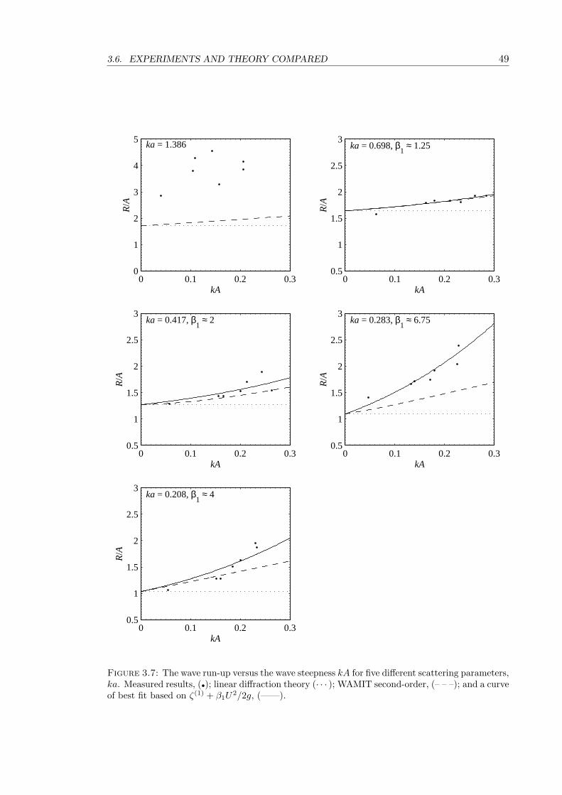
3.6. EXPERIMENTS AND THEORY COMPARED 49
0 0.1 0.2 0.30
1
2
3
4
5
kA
R/A
ka = 1.386
0 0.1 0.2 0.30.5
1
1.5
2
2.5
3
kA
R/A
ka = 0.698, β1 ≈ 1.25
0 0.1 0.2 0.30.5
1
1.5
2
2.5
3
kA
R/A
ka = 0.417, β1 ≈ 2
0 0.1 0.2 0.30.5
1
1.5
2
2.5
3
kA
R/A
ka = 0.283, β1 ≈ 6.75
0 0.1 0.2 0.30.5
1
1.5
2
2.5
3
kA
R/A
ka = 0.208, β1 ≈ 4
Figure 3.7: The wave run-up versus the wave steepness kA for five different scattering parameters,ka. Measured results, (•); linear diffraction theory (· · · ); WAMIT second-order, (– – –); and a curveof best fit based on ζ(1) + β1U
2/2g, (——).

50 CHAPTER 3. WAVE RUN-UP ON A CIRCULAR CYLINDER
vertical water displacements on the column surface and are of most interest to designers.Over the complete range of (ka, kA) combinations considered, the linear diffraction
solution of Havelock (1940) does not perform well. This observation is not new (seeIsaacson, 1978; Kriebel, 1992a, for instance). The first-order solution demonstrates no kA
dependence. Consequently, the error in the first-order prediction monotonically increasesfor increasing kA. This error is of order 20% and 100% in large values of kA for ka = 0.698and 0.208 respectively.
On the other hand, the first-order prediction of Havelock (1940) does realise a rea-sonable agreement with the measured results for very small kA (kA ≈ 0.05 for instance).This indicates that at such a small wave steepness incident wave non-linearities are notimportant and that local wave diffraction is confined to the first-harmonic. The decom-position of the wave run-up into harmonic proportions (cf. §2.5.3) suggests this to be so.It is reasonable to suggest that the wave run-up, regardless of ka, approaches the lineardiffraction solution as kA → 0. This is an important and fundamental result.
This under prediction by linear diffraction theory is somewhat arrested by the inclusionof second-order terms, where non-linearities of O(kA2) are accounted for. Perhaps this isbest illustrated by the results pertaining to ka = 0.698, where the WAMIT second-ordersolution agrees favourably with the measured wave run-up up to, and including, kA ≈ 0.25.However, we can see that as the incident wave becomes longer (ka decreases) non-lineareffects from incident wave steepness occur at increasingly smaller values of kA. In a sensethis could be described a ‘threshold’ for extreme, or higher than second-order, non-lineareffects associated with kA. At this threshold the normalised measured values are seento depart from the second-order perturbation predictions (cf. Figure 3.7 for ka = 0.417and 0.208). The measured values are then seen to follow an nth degree polynomial trend.This possibly indicates the existence of higher-order contributions to the wave run-up.Furthermore, it also suggests that proposed limitations regarding the validity of Stokesperturbation for free waves (Chakrabarti, 1987; Fenton, 1990), in water of infinite depth,based strictly on kA are essentially invalid when wave-structure interaction is considered.This is evidenced by Figure 3.7, where the measured results clearly indicate that the kA
limit is closely coupled with ka. A higher-order or fully non-linear representation of thevelocity potential may produce a better agreement with the measured results for large kA.
The dependence of the normalised wave run-up on the wave steepness was not demon-strated for the shortest waves tested. For ka = 1.386 in particular, the normalisationof the wave run-up with the first-harmonic of the incident wave produced some extremeamplifications of around four times the incident wave amplitude. Such extreme amplifi-cations are not predicted by second-order perturbation theory. As suggested earlier, thewave run-up for this particular value of ka exhibited a pseudo build-up every few wave pe-riods. This, coupled with the general scatter in the data, further suggests that generating,quality, high frequency monochromatic waves is difficult. The other main departure ofthe measured results from second-order theory is shown for ka = 0.283. This discrepancyshall be addressed in the harmonic analysis of the wave run-up.
When examining the actual wave run-up, it is also important to consider measurementsof the free-surface elevation in the fluid domain surrounding the cylinder. The maximum
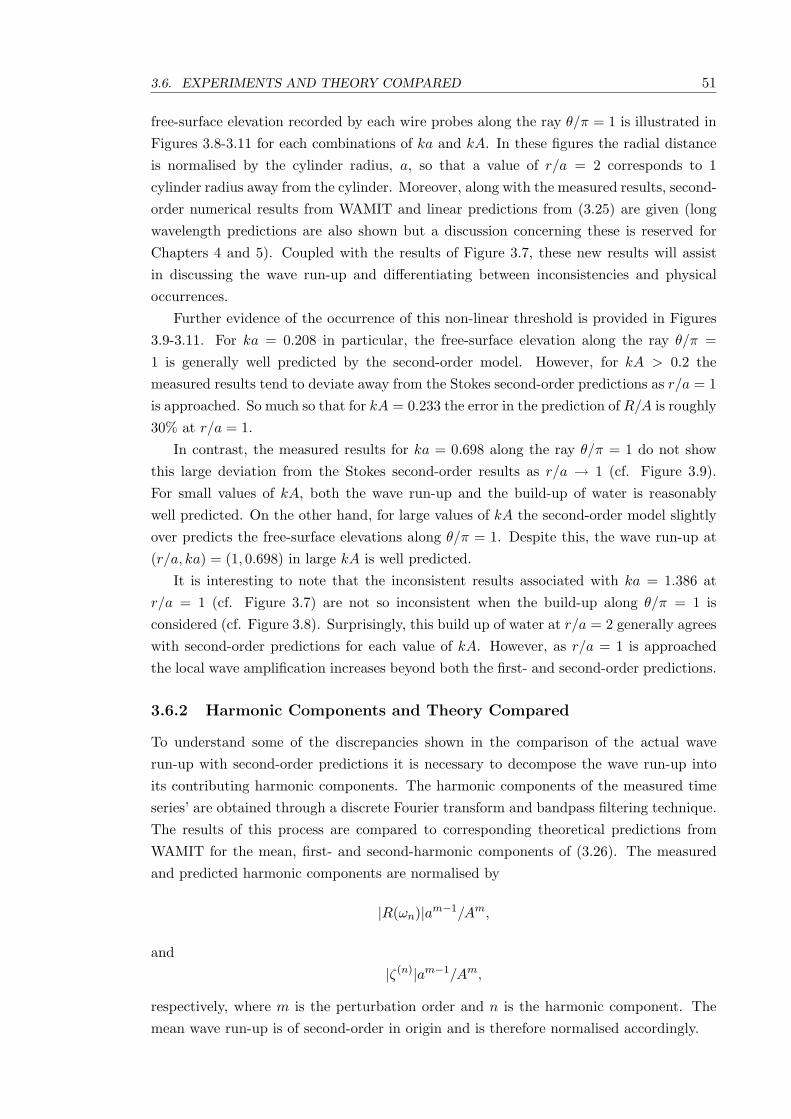
3.6. EXPERIMENTS AND THEORY COMPARED 51
free-surface elevation recorded by each wire probes along the ray θ/π = 1 is illustrated inFigures 3.8-3.11 for each combinations of ka and kA. In these figures the radial distanceis normalised by the cylinder radius, a, so that a value of r/a = 2 corresponds to 1cylinder radius away from the cylinder. Moreover, along with the measured results, second-order numerical results from WAMIT and linear predictions from (3.25) are given (longwavelength predictions are also shown but a discussion concerning these is reserved forChapters 4 and 5). Coupled with the results of Figure 3.7, these new results will assistin discussing the wave run-up and differentiating between inconsistencies and physicaloccurrences.
Further evidence of the occurrence of this non-linear threshold is provided in Figures3.9-3.11. For ka = 0.208 in particular, the free-surface elevation along the ray θ/π =1 is generally well predicted by the second-order model. However, for kA > 0.2 themeasured results tend to deviate away from the Stokes second-order predictions as r/a = 1is approached. So much so that for kA = 0.233 the error in the prediction of R/A is roughly30% at r/a = 1.
In contrast, the measured results for ka = 0.698 along the ray θ/π = 1 do not showthis large deviation from the Stokes second-order results as r/a → 1 (cf. Figure 3.9).For small values of kA, both the wave run-up and the build-up of water is reasonablywell predicted. On the other hand, for large values of kA the second-order model slightlyover predicts the free-surface elevations along θ/π = 1. Despite this, the wave run-up at(r/a, ka) = (1, 0.698) in large kA is well predicted.
It is interesting to note that the inconsistent results associated with ka = 1.386 atr/a = 1 (cf. Figure 3.7) are not so inconsistent when the build-up along θ/π = 1 isconsidered (cf. Figure 3.8). Surprisingly, this build up of water at r/a = 2 generally agreeswith second-order predictions for each value of kA. However, as r/a = 1 is approachedthe local wave amplification increases beyond both the first- and second-order predictions.
3.6.2 Harmonic Components and Theory Compared
To understand some of the discrepancies shown in the comparison of the actual waverun-up with second-order predictions it is necessary to decompose the wave run-up intoits contributing harmonic components. The harmonic components of the measured timeseries’ are obtained through a discrete Fourier transform and bandpass filtering technique.The results of this process are compared to corresponding theoretical predictions fromWAMIT for the mean, first- and second-harmonic components of (3.26). The measuredand predicted harmonic components are normalised by
|R(ωn)|am−1/Am,
and|ζ(n)|am−1/Am,
respectively, where m is the perturbation order and n is the harmonic component. Themean wave run-up is of second-order in origin and is therefore normalised accordingly.

52 CHAPTER 3. WAVE RUN-UP ON A CIRCULAR CYLINDER
1 1.2 1.4 1.6 1.8 2
1
2
3
4
5
r / a
R /
A
ka = 1.386, kA = 0.206
1 1.2 1.4 1.6 1.8 2
1
2
3
4
5
r / a
R /
A
ka = 1.386, kA = 0.206
1 1.2 1.4 1.6 1.8 2
1
2
3
4
5
r / a
R /
A
ka = 1.386, kA = 0.143
1 1.2 1.4 1.6 1.8 2
1
2
3
4
5
r / a
R /
A
ka = 1.386, kA = 0.157
1 1.2 1.4 1.6 1.8 2
1
2
3
4
5
r / a
R /
A
ka = 1.386, kA = 0.109
1 1.2 1.4 1.6 1.8 2
1
2
3
4
5
r / a
R /
A
ka = 1.386, kA = 0.104
1 1.2 1.4 1.6 1.8 2
1
2
3
4
5
r / a
R /
A
ka = 1.386, kA = 0.041
Figure 3.8: Circular Cylinder, rc/a = 1: The normalised wave elevation in the near field, atθ/π = 1, versus r/a. Measured values are given by the solid line with (•); First-order calculations,(– – –); Second-order calculations, (——); Second-order LWL calculations, (– · –).

3.6. EXPERIMENTS AND THEORY COMPARED 53
1 1.2 1.4 1.6 1.8 20.5
1
1.5
2
2.5
r / a
R /
A
ka = 0.698, kA = 0.284
1 1.2 1.4 1.6 1.8 20.5
1
1.5
2
2.5
r / a
R /
A
ka = 0.698, kA = 0.261
1 1.2 1.4 1.6 1.8 20.5
1
1.5
2
2.5
r / a
R /
A
ka = 0.698, kA = 0.233
1 1.2 1.4 1.6 1.8 20.5
1
1.5
2
2.5
r / a
R /
A
ka = 0.698, kA = 0.212
1 1.2 1.4 1.6 1.8 20.5
1
1.5
2
2.5
r / a
R /
A
ka = 0.698, kA = 0.179
1 1.2 1.4 1.6 1.8 20.5
1
1.5
2
2.5
r / a
R /
A
ka = 0.698, kA = 0.162
1 1.2 1.4 1.6 1.8 20.5
1
1.5
2
2.5
r / a
R /
A
ka = 0.698, kA = 0.062
Figure 3.9: Circular Cylinder, rc/a = 1: The normalised wave elevation in the near field, atθ/π = 1, versus r/a. Measured values are given by the solid line with (•); First-order calculations,(– – –); Second-order calculations, (——); Second-order LWL calculations, (– · –).

54 CHAPTER 3. WAVE RUN-UP ON A CIRCULAR CYLINDER
1 1.2 1.4 1.6 1.8 20.5
1
1.5
2
2.5
r / a
R /
A
ka = 0.417, kA = 0.263
1 1.2 1.4 1.6 1.8 20.5
1
1.5
2
2.5
r / a
R /
A
ka = 0.417, kA = 0.244
1 1.2 1.4 1.6 1.8 20.5
1
1.5
2
2.5
r / a
R /
A
ka = 0.417, kA = 0.213
1 1.2 1.4 1.6 1.8 20.5
1
1.5
2
2.5
r / a
R /
A
ka = 0.417, kA = 0.2
1 1.2 1.4 1.6 1.8 20.5
1
1.5
2
2.5
r / a
R /
A
ka = 0.417, kA = 0.166
1 1.2 1.4 1.6 1.8 20.5
1
1.5
2
2.5
r / a
R /
A
ka = 0.417, kA = 0.156
1 1.2 1.4 1.6 1.8 20.5
1
1.5
2
2.5
r / a
R /
A
ka = 0.417, kA = 0.057
Figure 3.10: Circular Cylinder, rc/a = 1: The normalised wave elevation in the near field, atθ/π = 1, versus r/a. Measured values are given by the solid line with (•); First-order calculations,(– – –); Second-order calculations, (——); Second-order LWL calculations, (– · –).

3.6. EXPERIMENTS AND THEORY COMPARED 55
1 1.2 1.4 1.6 1.8 20.5
1
1.5
2
2.5
r / a
R /
A
ka = 0.208, kA = 0.233
1 1.2 1.4 1.6 1.8 20.5
1
1.5
2
2.5
r / a
R /
A
ka = 0.208, kA = 0.231
1 1.2 1.4 1.6 1.8 20.5
1
1.5
2
2.5
r / a
R /
A
ka = 0.208, kA = 0.2
1 1.2 1.4 1.6 1.8 20.5
1
1.5
2
2.5
r / a
R /
A
ka = 0.208, kA = 0.185
1 1.2 1.4 1.6 1.8 20.5
1
1.5
2
2.5
r / a
R /
A
ka = 0.208, kA = 0.16
1 1.2 1.4 1.6 1.8 20.5
1
1.5
2
2.5
r / a
R /
A
ka = 0.208, kA = 0.152
1 1.2 1.4 1.6 1.8 20.5
1
1.5
2
2.5
r / a
R /
A
ka = 0.208, kA = 0.055
Figure 3.11: Circular Cylinder, rc/a = 1: The normalised wave elevation in the near field, atθ/π = 1, versus r/a. Measured values are given by the solid line with (•); First-order calculations,(– – –); Second-order calculations, (——); Second-order LWL calculations, (– · –).

56 CHAPTER 3. WAVE RUN-UP ON A CIRCULAR CYLINDER
3.6.2.1 Zero-Harmonic
This comparison, for the zero-harmonic wave run-up component, is illustrated in Figure3.12. Generally, the measured results exhibit some scatter which appears to decrease forincreasing wavelength. Despite this, it is clearly shown that, over the complete range ofka and kA values considered, the predicted mean component greatly underestimates themeasured results.
In long waves, the measured zero-harmonic appears to increase with increasing wavesteepness (cf. Figure 3.12 with ka = 0.208 for instance). This indicates a higher thansecond-order wave steepness dependence. To account for this in a theoretical model, onewould require a fully-nonlinear treatment of the free-surface boundary condition or, at theleast, a diffraction theory correct to fourth-order in Stokes perturbation.
It should also be noted that the undisturbed incident waves contained a small zero-harmonic component. In complex form the zero-harmonic contained a phase of either ±π.Although this mean component is obviously physical, its origin is unclear since accord-ing to Bernoulli’s theorem applied at the free-surface position the mean wave componentshould be zero for a free wave with corresponding locked harmonic components. Althoughit is possible that the datum for each wave probe drifted, this seems unlikely consideringthat the datum was recorded before each test run. Correcting for this non-zero mean didnot affect the recorded free-surface elevations substantially and the large discrepancies ob-served in the mean component of Figure 3.12 remain. Recently, observation by Stansberg& Braaten (2002) have confirmed the existence of a large zero-harmonic component thatis not well predicted by WAMIT computations.
3.6.2.2 First-Harmonic
The modulus and phase of the first-harmonic of the wave run-up are illustrated in Figures3.13 and 3.14 respectively. In both Figures, the predicted values are obtained from thelinear diffraction theory of Havelock (1940). For this particular harmonic, good compar-isons with theoretical predictions are observed since the measured values show very littlescatter.
Apart from when ka = 0.283 and ka = 1.386 the modulus and phase of R(ω1) agreeswell with theory. The scatter shown for the case of ka = 1.386 is expected since thequality of these waves was poor as previously discussed. However, for results pertainingto ka = 0.283 it is obvious that another attributing factor is forced at the first-harmonicsince for all kA values the under-estimation by theory is constant and of approximately20%. This discrepancy, however, does not carry through to the phase of R(ω1) since it isreasonably well predicted by theory (cf. Figure 3.14). A possible cause of this discrepancyis the excitation of a wave tank resonant mode. This will be discussed later.
It is important to note that previous authors have noted large discrepancies whencomparing the linear diffraction solution of MacCamy & Fuchs (1954) to the complete waverun-up (see Martin et al., 2001; Niedzwecki & Duggal, 1992, for instance). Here however,the linear diffraction solution, which contains only the fundamental wave frequency, iscompared only to the first-harmonic component of the wave run-up. In doing this and

3.6. EXPERIMENTS AND THEORY COMPARED 57
0 0.025 0.05 0.075 0.1 0.125 0.15 0.175 0.2 0.225 0.25 0.275 0.30
2
4
6
8|R
(ω0)|
a / A
2ka = 1.386
0 0.025 0.05 0.075 0.1 0.125 0.15 0.175 0.2 0.225 0.25 0.275 0.30
0.25
0.5
0.75
1
|R(ω
0)| a
/ A2
ka = 0.698
0 0.025 0.05 0.075 0.1 0.125 0.15 0.175 0.2 0.225 0.25 0.275 0.30
0.25
0.5
0.75
1
|R(ω
0)| a
/ A2
ka = 0.417
0 0.025 0.05 0.075 0.1 0.125 0.15 0.175 0.2 0.225 0.25 0.275 0.30
0.25
0.5
0.75
1
|R(ω
0)| a
/ A2
ka = 0.283
0 0.025 0.05 0.075 0.1 0.125 0.15 0.175 0.2 0.225 0.25 0.275 0.30
0.25
0.5
0.75
1
|R(ω
0)| a
/ A2
ka = 0.208
kA
Figure 3.12: The normalised modulus of mean component of the wave run-up |R(ω0)| plottedagainst wave steepness kA. Measured results, (•); and WAMIT, (——).

58 CHAPTER 3. WAVE RUN-UP ON A CIRCULAR CYLINDER
0 0.025 0.05 0.075 0.1 0.125 0.15 0.175 0.2 0.225 0.25 0.275 0.30
0.5
1
1.5
2
2.5
|R(ω
1)| / A
ka = 1.386
0 0.025 0.05 0.075 0.1 0.125 0.15 0.175 0.2 0.225 0.25 0.275 0.30
0.5
1
1.5
2
2.5
|R(ω
1)| / A
ka = 0.698
0 0.025 0.05 0.075 0.1 0.125 0.15 0.175 0.2 0.225 0.25 0.275 0.30
0.5
1
1.5
2
2.5
|R(ω
1)| / A
ka = 0.417
0 0.025 0.05 0.075 0.1 0.125 0.15 0.175 0.2 0.225 0.25 0.275 0.30
0.5
1
1.5
2
2.5
|R(ω
1)| / A
ka = 0.283
0 0.025 0.05 0.075 0.1 0.125 0.15 0.175 0.2 0.225 0.25 0.275 0.30
0.5
1
1.5
2
2.5
|R(ω
1)| / A
ka = 0.208
kA
Figure 3.13: The normalised modulus of first-harmonic component of the wave run-up |R(ω1)|plotted against wave steepness kA. Measured results, (•); and Linear diffraction solution, (——).

3.6. EXPERIMENTS AND THEORY COMPARED 59
0 0.025 0.05 0.075 0.1 0.125 0.15 0.175 0.2 0.225 0.25 0.275 0.3−1
0
1
2
3A
rg(R
(ω1))
ka = 1.386
0 0.025 0.05 0.075 0.1 0.125 0.15 0.175 0.2 0.225 0.25 0.275 0.3−1
0
1
2
3
Arg
(R(ω
1))
ka = 0.698
0 0.025 0.05 0.075 0.1 0.125 0.15 0.175 0.2 0.225 0.25 0.275 0.3−1
0
1
2
3
Arg
(R(ω
1))
ka = 0.417
0 0.025 0.05 0.075 0.1 0.125 0.15 0.175 0.2 0.225 0.25 0.275 0.3−1
0
1
2
3
Arg
(R(ω
1))
ka = 0.283
0 0.025 0.05 0.075 0.1 0.125 0.15 0.175 0.2 0.225 0.25 0.275 0.3−1
0
1
2
3
Arg
(R(ω
1))
ka = 0.208
kA
Figure 3.14: The Phase of first-harmonic component of the wave run-up Arg(R(ω1)) plottedagainst wave steepness kA. Measured results, (•); and Linear diffraction solution, (——).

60 CHAPTER 3. WAVE RUN-UP ON A CIRCULAR CYLINDER
distinguishing between the coupling of ka and kA, the results indicate that the lineardiffraction solution performs extremely well by capturing both the modulus and phase ofthe first-harmonic wave run-up.
An interesting observation is seen for ka = 0.208 when the wave steepness reachesroughly 50% of the wave breaking limit. In this region, higher than second-order wavesteepness effects appear to be operating at the first-harmonic since the measured resultsindicate a relatively consistent increase in |R(ω1)| for kA > 0.2. This possibly accountsfor the sharp increase in the wave run-up noted in the discussion pertaining to Figure 3.7(cf. §3.6.1).
It is important to mention that the finite depth of the towing tank has not affectedthe measured results. If finite depth effects were present, then these would be particularlysignificant for the cases where ka = 0.208. The good agreement of the measured resultwith the theoretical predictions when ka = 0.208 has demonstrated that the assumptionof infinite water depth in the analysis is indeed a valid one.
3.6.2.3 Second-Harmonic
A comparison of the measured second-harmonic with second-order calculations from WAMITis shown in Figures 3.15 and 3.16 for the modulus and phase respectively. The scatter ex-hibited by the data appears to steadily decrease as the wavelength increases. This can beattributed to the sampling rate where approximately 85 samples are recorded within thethe second-harmonic of ka = 0.208 whilst only 30 records were taken for ω2 of ka = 1.386.Despite this scatter, the measured results show a fairly constant relationship between thenormalised modulus and kA. Moreover, the agreement of the measured results with the-oretical predictions is best shown for ka = 0.283 and 0.208. In the longer waves we cansee that perturbation theory over-predicts the modulus of the second-harmonic. This isquite considerable for ka = 1.39 where the error in R(ω2) is about 50%. The source ofthis large discrepancy is unclear.
This constant trend (cf. Figure 3.15 for ka = 0.283 and 0.208), would indicate thatthe modulus of the second-harmonic of the wave run-up is relatively wave steepness in-dependent over the range of kA values considered in this study. Similarly, higher-ordereffects operating at the second-harmonic are not important and therefore the leadingsecond-order contribution in a Stokes expansion to O(A2) accounts for the majority of thesecond-harmonic. If wave steepness effects were noticeable, then one would expect themto be more prevalent in longer waves (ka = 0.208), however, the measured results do notshow this.
The corresponding phase of the second-harmonic shows much more variability (cf.Figure 3.16). In some cases, particularly small values of kA, the phase is not well predictedby second-order theory at all. Good agreement between measured and calculated resultsis shown for both ka = 0.208 and 0.283 when kA > 0.175, and for ka = 0.698 whenkA < 0.225. It is possible that higher-order effects are contributing to the phase of R(ω2)but it is difficult to postulate upon this point without more data values.

3.6. EXPERIMENTS AND THEORY COMPARED 61
0 0.025 0.05 0.075 0.1 0.125 0.15 0.175 0.2 0.225 0.25 0.275 0.30
0.25
0.5
0.75
1
1.25|R
(ω2)|
a / A
2
ka = 1.386
0 0.025 0.05 0.075 0.1 0.125 0.15 0.175 0.2 0.225 0.25 0.275 0.30
0.25
0.5
0.75
1
1.25
|R(ω
2)| a
/ A2
ka = 0.698
0 0.025 0.05 0.075 0.1 0.125 0.15 0.175 0.2 0.225 0.25 0.275 0.30
0.25
0.5
0.75
1
1.25
|R(ω
2)| a
/ A2
ka = 0.417
0 0.025 0.05 0.075 0.1 0.125 0.15 0.175 0.2 0.225 0.25 0.275 0.30
0.25
0.5
0.75
1
1.25
|R(ω
2)| a
/ A2
ka = 0.283
0 0.025 0.05 0.075 0.1 0.125 0.15 0.175 0.2 0.225 0.25 0.275 0.30
0.25
0.5
0.75
1
1.25
|R(ω
2)| a
/ A2
ka = 0.208
kA
Figure 3.15: The normalised modulus of second-harmonic component of the wave run-up |R(ω2)|plotted against wave steepness kA. Measured results, (•); and WAMIT, (——).
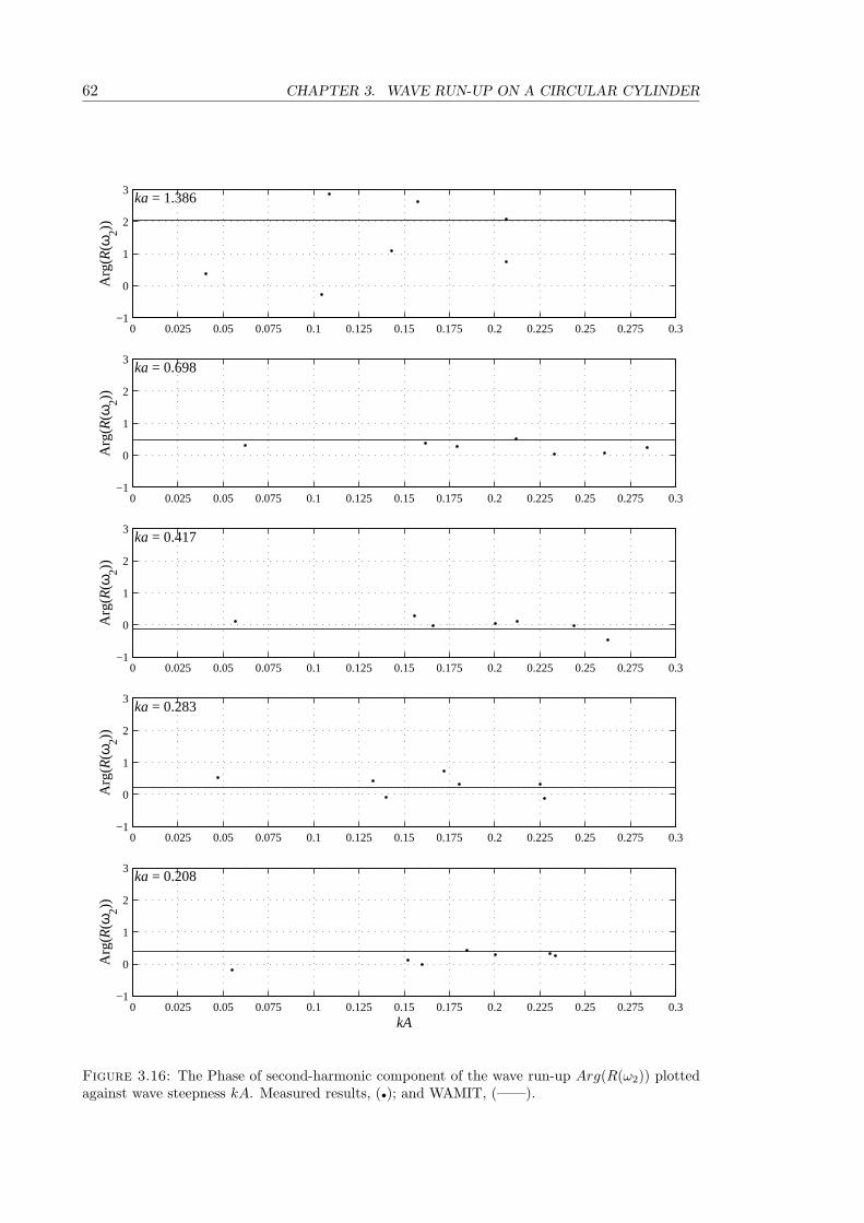
62 CHAPTER 3. WAVE RUN-UP ON A CIRCULAR CYLINDER
0 0.025 0.05 0.075 0.1 0.125 0.15 0.175 0.2 0.225 0.25 0.275 0.3−1
0
1
2
3
Arg
(R(ω
2))
ka = 1.386
0 0.025 0.05 0.075 0.1 0.125 0.15 0.175 0.2 0.225 0.25 0.275 0.3−1
0
1
2
3
Arg
(R(ω
2))
ka = 0.698
0 0.025 0.05 0.075 0.1 0.125 0.15 0.175 0.2 0.225 0.25 0.275 0.3−1
0
1
2
3
Arg
(R(ω
2))
ka = 0.417
0 0.025 0.05 0.075 0.1 0.125 0.15 0.175 0.2 0.225 0.25 0.275 0.3−1
0
1
2
3
Arg
(R(ω
2))
ka = 0.283
0 0.025 0.05 0.075 0.1 0.125 0.15 0.175 0.2 0.225 0.25 0.275 0.3−1
0
1
2
3
Arg
(R(ω
2))
ka = 0.208
kA
Figure 3.16: The Phase of second-harmonic component of the wave run-up Arg(R(ω2)) plottedagainst wave steepness kA. Measured results, (•); and WAMIT, (——).

3.6. EXPERIMENTS AND THEORY COMPARED 63
3.6.2.4 Third-Harmonic and Higher-Harmonic Components
Given the sampling length of the experiments, difficulty arose in obtaining an accurateextraction of the third-harmonic components as they are considerably smaller than bothfirst- and second-harmonics. Consequently, much scatter was shown for R(ω3) with ka =1.39 so only four of the five values of ka are presented in Figure 3.17.
The contribution from the third-harmonic to the wave run-up is indeed small. Whenthe onset of viscous effects is considered (A/a = 1), the measured results for ka = 0.208indicate that |R(ω3)| is around 0.1A. On the other hand, for A/a = 0.5 the measuredresults indicate that |R(ω3)| will be around 0.025A. Consequently, only when the incidentwave amplitude is comparable to the cylinder radius, do third-harmonic effects becomeimportant to the wave run-up.
Although the modulus of the third-harmonic component is small, the results indicate afairly constant contribution over the range of wave steepnesses considered. One exceptionis, of course, when kA ≈ 0.05. At such a small value of kA the third-harmonic is expectedto be small and the measured results show a large contribution that increases with ka.These erroneous measurements are most likely a result of the very small magnitude of thethird-harmonic coupled with a limited frequency resolution in the DFT.
The phase of this third-harmonic (cf. Figure 3.18) shows a general decreasing trendwith increasing kA. This is particularly significant for short waves (ka = 0.698). However,the scatter exhibited in the measurements is quite extensive and thus not permitting anyqualitative conclusions. A more extensive study is required in order to gain valuableinformation on the behaviour of this third-harmonic contribution to the wave run-up.
3.6.2.5 Summary of Harmonic Components
To summarise the comparison of the measured and theoretical results for each harmoniccomponent, Table 3.3 illustrates the salient discrepancies expressed as a relative absoluteerror. The relation
|εr| = |RE(ωn)−RT (ωn)|RT (ωn)
,
is applied to each normalised harmonic component to express this error εr where RE andRT correspond to the experimental results and theoretical predictions respectively. Stokesperturbation to second-order suggests that the normalised modulus of each harmonic com-ponent is constant with kA. Although there are some exceptions, this is generally the caseand this assumption is invoked, with outliers removed, to provide the results of Table 3.3.With the results illustrated in this manner we can clearly see that the first-harmonic iswell predicted by linear diffraction theory and the second-harmonic is only well predictedin long waves. The zero-harmonic of the wave run-up is poorly predicted for each value ofka.

64 CHAPTER 3. WAVE RUN-UP ON A CIRCULAR CYLINDER
0 0.025 0.05 0.075 0.1 0.125 0.15 0.175 0.2 0.225 0.25 0.275 0.30
0.2
0.4
0.6
0.8
|R(ω
3)| a2 /
A3
ka = 0.698
0 0.025 0.05 0.075 0.1 0.125 0.15 0.175 0.2 0.225 0.25 0.275 0.30
0.2
0.4
0.6
0.8
|R(ω
3)| a2 /
A3
ka = 0.417
0 0.025 0.05 0.075 0.1 0.125 0.15 0.175 0.2 0.225 0.25 0.275 0.30
0.2
0.4
0.6
0.8
|R(ω
3)| a2 /
A3
ka = 0.283
0 0.025 0.05 0.075 0.1 0.125 0.15 0.175 0.2 0.225 0.25 0.275 0.30
0.2
0.4
0.6
0.8
|R(ω
3)| a2 /
A3
ka = 0.208
kA
Figure 3.17: The normalised modulus of third-harmonic component of the wave run-up |R(ω3)|plotted against wave steepness kA.

3.6. EXPERIMENTS AND THEORY COMPARED 65
0 0.025 0.05 0.075 0.1 0.125 0.15 0.175 0.2 0.225 0.25 0.275 0.3−3.5
−1.75
0
1.75
3.5A
rg(R
(ω3))
ka = 0.698
0 0.025 0.05 0.075 0.1 0.125 0.15 0.175 0.2 0.225 0.25 0.275 0.3−3.5
−1.75
0
1.75
3.5
Arg
(R(ω
3))
ka = 0.417
0 0.025 0.05 0.075 0.1 0.125 0.15 0.175 0.2 0.225 0.25 0.275 0.3−3.5
−1.75
0
1.75
3.5
Arg
(R(ω
3))
ka = 0.283
0 0.025 0.05 0.075 0.1 0.125 0.15 0.175 0.2 0.225 0.25 0.275 0.3−3.5
−1.75
0
1.75
3.5
Arg
(R(ω
3))
ka = 0.208
kA
Figure 3.18: The phase of third-harmonic component of the wave run-up Arg(R(ω3)) plottedagainst wave steepness kA.

66 CHAPTER 3. WAVE RUN-UP ON A CIRCULAR CYLINDER
Table 3.3: The absolute relative error, |εr| of the experimental results relative to theoreticalpredictions for the zero- first- and second-harmonic components of the wave run-up. RE and RT
are the experimental and theoretical predictions of the wave run-up respectively.
ka ω0 ω1 ω2
|RE −RT | |εr| |RE −RT | |εr| |RE −RT | |εr|1.386 4.542 4.652 0.302 0.176 0.543 0.5110.698 0.358 0.793 0.117 0.072 0.138 0.2320.417 0.198 1.222 0.015 0.012 0.178 0.2750.283 0.317 3.885 0.240 0.219 0.018 0.0340.208 0.115 2.163 0.039 0.038 0.036 0.103
3.6.3 Regression Analysis
From the comparisons of the zero- first- and second-harmonic harmonic components withperturbation theory, it appears that the first-order diffraction solution predicts the first-harmonic contribution to the wave run-up reasonably well. On the other hand, the second-order solution fails to capture the zero- and second- harmonic components effectively overa sufficient range of ka and kA values. Given this, the first-order solution can form a basisupon which to build a preliminary wave run-up investigation.
An approach suggested by Hallermeier (1976) is the so called velocity-head method,where the wave run-up can be approximated by the equation
R
A= β0 + β1
U2
2gA. (3.31)
The first term, β0 is an additive constant which is usually given as the wave amplitudeat the up-wave side of the column, β1 is a constant of proportionality, and U2/2gA is theFroude number or the non-dimensional velocity squared term from Bernoulli’s equationapplied at the free-surface. The last part of (3.31) implies that the horizontal waterparticle velocity is transferred to the vertical direction when water impacts on a boundary.Previous authors have employed (3.31) (see Martin et al., 2001; Niedzwecki & Huston,1992) to estimate the wave run-up with limited success, mainly because of experimentalscatter resulting from wave steepness effects on the wave run-up.
Here however, we separate the coupling of ka and kA by taking the limiting value ofthe wave run-up as kA → 0. This produces the linear diffraction solution of Havelock, andis used to replace the coefficient β0 in (3.31). By this we are implying that all diffraction isconfined to first-order or alternatively the first-harmonic and that wave steepness effectsare confined to the velocity squared component in (3.31). This U2 term can therefore bethought of as a correction to the fundamental diffraction solution due to the jet of waterrushing up the column. The horizontal velocity term, U , is taken from linear theory witha correction to second-order from Stokes drift (see Newman, 1977, equation 6.47), thusproducing terms of O(A4). Applying these assumptions to (3.31), the equation for the

3.7. SOME COMMENTS ON DISCREPANCIES 67
regression analysis becomes
R
A=|ζ(1)|
A+ β1[12kA + (kA)2 + 1
2(kA)3], (3.32)
where β1 is chosen for the least square fit to the data in Figure 3.7. These assumptionsdiffer from those of previous authors where one specific value for the coefficients β0 and β1
were selected, see Haney & Herbich (1982) and Niedzwecki & Huston (1992) for instancewhere β1 = 1 and 6.52 respectively. In particular, results from these authors demon-strate significant experimental scatter with no clear trends because the wave run-up is notdecomposed into wave frequency and wave steepness effects.
The application of (3.32) for the regression analysis in Figure 3.7 captures the run-uptrends for ka = 0.698, 0.417 and 0.283 where β1 = 1.25, 2 and 6.75 respectively. Thissystematic increase in β1 with ka implies that non-linearities increase with longer wave-lengths. As suggested earlier, the wave run-up does indeed follow an nth degree polynomialtrend with kA. However, for the longest wave, ka = 0.208 the regression curve fails tocapture the trend for large kA particulary well. In this case the polynomial dependenceon kA is much stronger, possibly because third-harmonic wave components and resultingthird-order diffraction effects, which operate at both the first- and third-harmonics, be-come important here (cf. Figure 2.7). The comparison illustrates that the wave run-upexhibits a higher-order dependence on kA which is particularly significant for long wave-lengths. This trend is not captured by a perturbation scheme correct to second-order inwave steepness.
3.7 Some Comments on Discrepancies
We have examined the harmonic components of the wave run-up to identify causes of dis-crepancies between measured results and a Stokes perturbation scheme correct to second-order in kA. However, some aspects of the data analysis and the experimental campaignshould be discussed in order to bring to attention other sources of error.
The signal length recorded from the wire probes could offer a possible explanation forthe poor resolution of some Fourier components. An example where the signal length mayhave affected the resolution of each harmonic is demonstrated by the scatter shown for ω2
in short waves (see Figure 3.15 for ka = 0.417 and 0.698 for instance). In each instanceexactly 10 wave periods were used in the Fourier analysis. The primary reasons for thisrestriction are the avoidance of reflected waves from the beach and second-harmonic para-sitic waves generated at the wave maker. As a result, the frequency resolution in the DFTwas compromised. For instance, 10 waves of frequency ω = 6.76rads−1 produces a fre-quency resolution of fs = 0.09Hz in the frequency spectrum. Given that, the correspondingfirst- and second-harmonic of this wave would comprise frequencies of f1 = 1.07± 0.09Hzf2 = 2.15 ± 0.09Hz respectively. The exact position of these harmonics is limited by thefrequency resolution and thereby so are their magnitudes. This frequency band becomesincreasing significant when higher wave harmonics are considered as their magnitude’s arevery small. Increasing the frequency resolution was not possible in the set of experiments

68 CHAPTER 3. WAVE RUN-UP ON A CIRCULAR CYLINDER
described here due to the limited length of the wave tank.Despite efforts in selecting the time window, it is quite possible that contamination
by free wave components of 2ω in the tail of the time series occurred. For the shortestwaves, no problem is encountered since 30 wave periods were recorded and the Fourieranalysis was subsequently performed over a selection of periods at the beginning of thetime series. However this judicious selection was not possible for long waves (ka = 0.208)as only 14 wave periods were available within the time window. If data recording hadcommenced concurrently with the ramp-up of the wave generation system, then an ap-propriate selection of the time series could have been chosen during post-processing usingFourier analysis to identify and avoid free-wave components.
The avoidance of wave tank resonance is extremely important during experimentsinvolving waves and external boundaries. Wave tank resonance is an extremely visualphenomenon and has been reported during experiments conducted at the University ofWestern Australia’s wave tank. When wave energy is provided at a resonant frequencycorresponding to cross-tank eigenmodes, only viscous effects can dampen out the oscilla-tions. It was previously pointed out that poor agreement between theory and measuredresults pertaining to ka = 0.283 could be attributed to the excitation of a wave tankresonant mode. The carrier wave frequency in this instance is f = 0.68Hz. Although itdoes not exactly correspond to the second-mode of wave tank resonance, predicted by therelation
fm =12π
√kmg, where km = πm/l: m ∈ Z+, (3.33)
it is relatively close. Since the bandwidth of the first-harmonic component was not asnarrow as expected some portion of the wave energy may have excited this resonant modeat f2 and therefore affecting the first-harmonic Fourier component of each wave wheref = 0.68Hz. The corresponding second-harmonic Fourier component of this carrier wavewas not affected and the comparison with theory is good. It was perhaps difficult toobserve resonance during the experiments since an absorbing beach was utilised after eachrun to dampen wave energy and thus reduce waiting times between runs. Wave tankresonance may offer some explanation for the poor correspondence of ka = 0.283 withtheory.
In regards to the numerical results it is important to note that the Green’s functionrepresentation in WAMIT is based on a fluid domain of infinite extent in the radial di-rection. This is commonly known as an open-sea Green’s function. Strictly speaking, theexperimental measurements are obtained within a domain bounded by zero-flux surfaceson both the tank bottom and side walls. Provided that resonant modes and side wall ef-fects do not contaminate the experimental result then comparisons with numerical resultsbased on an open sea Green’s function are justified. However, as we have seen here, aresonant mode has possibly been excited and in which case a more accurate comparisoncould be obtained by using a so called tank Green’s function (TFG) (see Chen, 1994; Xia,2001, for instance). The TGF satisfies the additional zero-flux boundary conditions on thesidewalls and can be used to deduce the influence of these sidewall effects on experimentalresults and indeed provide criteria to avoid resonant modes and sidewall reflections inexperiments.

3.8. CHAPTER SUMMARY 69
In experiments conducted by Armstrong & Haritos (1997) side-wall effects were thoughtto have enhanced wave run-up measurements. As suggested by Sarpkaya & Isaacson(1981), the ratio of tank width to cylinder diameter, l/(2a) should not be less than 2 ifside-wall and general blockage effects are to be avoided. Although this may be adequate forwave force measurements, it is generally too small for reliable free-surface elevation mea-surements. This is best demonstrated in experiments documented by Martin et al. (2001),where despite l/2a being 3.63, disturbances created from side wall effects completely ob-scured some of their wave run-up measurements. In our experiments l/2a = 11.8 and sidewall reflections are not thought to have contaminated the measured results.
3.8 Chapter Summary
The wave run-up has been separated, through appropriate use of dimensional analysis, intoka and kA effects. The second-order numerical results suggest that, despite large incidentwave amplifications in short waves, it is the intermediate to long waves that produce thehighest vertical water displacement on a cylindrical column. This is of course governed bythe influence of kA. The second-order analysis has revealed distinct wave run-up peaks,for a fixed column, occurring in the region ka < 1. The first peak occurs at ka ≈ 0.3and the run-up height is approximately 200% greater than that of the second peak whichoccurs at ka ≈ 0.9. The second-order numerical results suggest that the magnitude of thisincrease between ka ≈ 0.3 and 0.9 is relatively wave steepness independent.
Comparisons of the measured wave run-up with theory demonstrates that a second-order diffraction analysis can indeed produce reasonable predictions of the wave run-up.However, this is highly dependent upon both ka and kA. For smaller values of ka higher-order diffraction effects occur at increasingly smaller values of kA, and hence a higher-orderrepresentation of the velocity potential is required in order to capture these kA effects.
The harmonic analysis has shown that these higher-order effects appear to operate atthe first-harmonic for small values of ka and large values of kA. Consequently, in thisregion the linear diffraction solution of Havelock (1940) under predicts the contributionof the first-harmonic wave run-up component. However, when higher-order effects are notsignificant at the first-harmonic, the first-order solution compares favourably with mea-sured results. A unique regression analysis, with first-order diffraction effects accountedfor by the Havelock solution has produced a reasonable agreement with the experimentalresults. It has shown that the appropriate contribution from incident wave non-linearitiesis inversely proportional to local wave diffraction.

Chapter 4
Long Wavelength Approximation
Recently, attention has been paid to the extension of a perturbation type treatment of thenon-linear free-surface boundary condition to third-order in the work of Faltinsen, Newman& Vinje (1995) and Malenica & Molin (1995) for the scattering of monochromatic waves bya fixed surface piercing cylinder. This has been primarily stimulated by observations of theexcitation of resonant modes in offshore structures exhibiting high natural-frequencies byhigher-harmonic non-linear wave loads. This phenomena is commonly termed ‘ringing’ andhas been reported by Krokstad & Stansberg (1995), Chaplin et al. (1997) and others. Ofthe two perturbation schemes, both involve monochromatic waves of small wave steepness,however, the theory of Faltinsen, Newman & Vinje (1995) (hereafter referred to as ‘FNV’)is restricted to a/L ¿ 1 in water of infinite depth, while that of Malenica & Molin (1995)is based on classical Stokes perturbation and is valid for arbitrary wavelength and fluid offinite depth. Due to the restriction of a/L ¿ 1, the work of FNV is more appropriatelytermed a long wavelength (LWL) theory.
The work presented here shall extend the LWL theory of FNV to account for thefree-surface elevation to third-order in wave amplitude. The long wavelength theory formonochromatic waves incident on a vertical surface penetrating circular cylinder in waterof infinite depth is elucidated in §4.1. Certain aspects of this theory are discussed in §4.2pertaining to the magnitude and harmonic contributions of the various terms in the free-surface elevation expression. Finally, comparisons of the LWL theory with experimentaland numerical results are presented in §4.3.
4.1 Long Wavelength Theory
For wave-structure interaction problems in long waves, it is generally thought that classicaldiffraction theory, based on small wave steepness assumptions, may in fact be irrelevant.This is ostensibly because long waves can exhibit wave amplitudes that are of comparablemagnitude to the cross sectional dimensions of a platform column. As a consequence,the free-surface Keulegan-Carpenter number, Kc = πA/a, is of the order of π. This isclearly a violation of the classical Stokes perturbation approach, whereby the restrictionof Kc ¿ π is intrinsically assumed. With this in mind, FNV reconsiders the governingrelative length scales to the problem in a consistent fashion. Formally, one can write,kA = O(ε), ka = O(ε) and A/a = O(1). The restriction on ka essentially implies that the

72 CHAPTER 4. LONG WAVELENGTH APPROXIMATION
Figure 4.1: Schematic of the coordinate system adopted for long wavelength theory.
wavelengths is now considered. The resulting LWL potentials satisfy the homogeneousform of the exact free-surface boundary condition. To treat the non-linear free-surfaceboundary condition, the adopted perturbation scheme is defined in §4.1.2. Moreover, thisgives rise to two assisting non-linear potentials which are found by employing an integraltransform of the boundary value problem in §4.1.2. Of these two non-linear potentials, interms of a regular Stokes expansion, one is of O(A2) and the other is of O(A3). Finally, thefree-surface elevation correct to third-order in long wavelength assumptions is derived in§4.1.3 along with its corresponding simplification on r = a. It is the compact form of theexpression for the free-surface elevation on r = a which is of interest for an investigationinto wave run-up in long waves.
4.1.1 The Linear Diffraction Potential
The effects of viscosity are ignored and potential flow is assumed throughout a fluid ofinfinite depth. The coordinate system adopted for the problem is defined in Figure 4.1.In deep water, the well known incident wave potential from linear wave theory is
φ(1) = <{gA
ωexp(kz − ikx + iωt)
}, (4.1)
where the dispersion relation is defined by k = ω2/g and the direction of wave propagationis from x = −∞. Equation (4.1) is valid to O(A3) in water of infinite depth provided thatthe usual dispersion relation is corrected for amplitude dispersion. In this instance, itis replaced by the expression k0 = k(1 + k2A2) where k0 = ω2/g (see Newman, 1977,equation 6.39). This correction implies that the wave steepness exhibits an influence onphase velocity. In cylindrical coordinates, (r, θ, z) where x+iy = reiθ, (4.1) can be replaced

4.1. LONG WAVELENGTH THEORY 73
by the following incident wave potential
φI = <{
gA
ωe(kz+iωt)
∞∑
m=0
εmi−mJm (kr) cos mθ
}, (4.2)
where ε0 = 1 and εm = 2 for m > 0 and Jm is the Bessel function of order m. In thepresence of a vertical surface piercing cylinder, the corresponding scattered potential iswritten
φS = −<{
gA
ωe(kz+iωt)
∞∑
m=0
εmi−m H(2)m (kr)J ′m(ka)
H(2)′m (ka)
cosmθ
}, (4.3)
where the coefficients of this eigenfunction expansion are chosen to satisfy the zero fluxboundary condition at the cylinder surface. The Hankel function of the second kind ischosen to represent outgoing waves. The addition of the incident and scattered potentialsgives
φ(1) = <{
gA
ωe(kz+iωt)
∞∑
m=0
εmi−mCm(kr) cos mθ
}, (4.4)
where
Cm(kr) = Jm(kr)− J′m(ka)
H(2)′m (ka)
H(2)m (kr), (4.5)
which is the classical linear-diffraction potential for water of infinite depth presented byHavelock (1940, equation 17). Following Lighthill (1979), when both ka and kr are con-sidered small the first three terms of the series containing combinations of Bessel andHankel functions (4.5) dominates when expanded with respect to their arguments. In thisinstance, (4.4) can be rewritten in the following approximate form
φ(1) = <{gA
ωe(kz+iωt)(C0(kr)− 2iC1(kr) cos θ − 2C2(kr) cos 2θ)
}. (4.6)
where
C0(kr) = 1 + 12(ka)2(ln 1
2kr + γ + πi/2)− 14(kr)2 +O((kr)4, (kr)4 log kr), (4.7)
C1(kr) =k
2
(r +
a2
r
)+O((kr)3, (kr)3 log kr), (4.8)
and
C2(kr) =k
8
(r2 +
a4
r2
)+O((kr)4), (4.9)
where γ is understood to be the Euler-Mascheroni constant and has the numerical valueγ = 0.57722 to five significant figures. Since only the first few terms of the infinite serieswere retained we have implicity implied that r = O(a) and therefore this systematicexpansion is only valid in this neighbourhood. This neighbourhood can be thought of asan inner domain. The expansion (4.6) is essentially a coordinate perturbation in terms ofkr and is correct to order A(kr)2 and A(kr)2 log kr. In this long wavelength regime, theincident wave elevation is effectively phase independent and can be simply obtained from

74 CHAPTER 4. LONG WAVELENGTH APPROXIMATION
the first term of (4.7) in (4.6), whence
ζ1 = A sinωt. (4.10)
The form of (4.6) is not new and bears resemblance to that presented by Lighthill (1979,equation 72). It is worth noting that the systematic expansion of the infinite sum in (4.4)essentially gives rise to singularities analogous to the description of an oscillatory flow inthe presence of a circular plate at depth z. The addition of the first term in C0(kr) andC1(kr) in (4.6) represents an incident flow and its corresponding dipole response. The formof the second and last terms of C0(kr) together with C2(kr) in (4.6) represents the flow’sfluctuating extension and contains both a monopole and quadrupole response respectively(see Lighthill, 1979, figure 28).
4.1.2 The Non-Linear Potentials
Attention is now turned to the non-linear potentials that must assist (4.6) in the innerdomain of r = O(a). To derive these one must examine the free-surface boundary conditionand a suitable perturbation scheme. The exact free-surface boundary condition for an air-water interface (ignoring the effects of surface tension) is given by
φtt + gφz = −2∇φ · ∇φt − 12∇φ · ∇ (∇φ)2 , on z = ζ. (4.11)
The velocity potential defined by (4.6) satisfies the homogeneous form of (4.11) whenprescribed on z = 0. It is therefore strictly linear in terms of a classical Stokes perturbationscheme.
To evaluate the non-linear forcing of the right-hand side of (4.11), it is convenient toexpress φ in terms of a convergent power series with coefficients {εn; n = 1, 2, 3, . . . , }. Thisallows for a procedure of iteration by direct substitution of the expression for φ into (4.11)and equating for like powers of ε. In the conventional approach of infinitesimal or Stokeswave theory one usually selects ε to be the wave steepness, kA, and the characteristicdimensions of the cylinder relative to the incident wavelength to be of O(1). This impliesthat Kc ¿ 1.
In contrast, the approach presented here proposes that the incident wavelength is largerelative to the cylinder dimensions and therefore the additional requirement of ka = O(ε)must be considered. As a result of this assumption, the representative Kc number is ofO(1). This prompts the choice of two perturbation parameters that represent parameterand coordinate expansions respectively
ε1 = kA and ε2 = ka, (4.12)
where both parameters are of order ε. This implies that the product of the two producesterms of O(εm
1 εn2 ) = O(εm+n). The following power series expansion for the velocity
potential correct to third-order in ε is now considered
φ(r, z, θ, t) = ε1ϕ1 + ε1ε2ϕ2 + ε1ε22ϕ3 + ε2
1ε2ψI + ε3
1ψII +O(ε4), (4.13)

4.1. LONG WAVELENGTH THEORY 75
The first few terms of this series are linear quantities in terms of a regular Stokes expansionin kA and may therefore be determined by equating like powers of O(ε1), O(ε1ε2) andO(ε1ε
22) from the coordinate series expansion given by (4.6). The following expressions for
ϕ1, ϕ2 and ϕ3 are then emitted
ϕ1 =ω
k2ekz cosωt, (4.14)
ϕ2 =ω
k2ekz sinωt
(r
a+
a
r
)cos θ, (4.15)
and
ϕ3 =ω
k2ekz+iωt
[12
(ln 1
2kr + γ +πi
2
)− 1
4
(r2
a2− cos 2θ
(r2
a2+
a2
r2
))]. (4.16)
It is now understood that φn = ε1εn−12 ϕn for positive integer n. Moreover, it is important
to note the distinction between the notation of the perturbed velocity potential from longwavelength theory and the conventional Stokes approach. For clarity, in this work, eachis denoted φn and φ(n) respectively.
The coefficients of these three potentials given by (4.14), (4.15) and (4.16) containterms involving A, Aa and Aa2. In order to obtain the correct long wavelength expansionto O(ε3), as seen in the expansion (4.13), the remaining contributions of O(A2a) andO(A3) must be determined. These remaining contributions are non-linear in terms of ε1
and are found by solving a BVP for ψI and ψII . These potentials complete the problemto O(ε3).
4.1.2.1 The Free-Surface Boundary Condition
To solve for ψI and ψII , the equations (4.14), (4.15) and (4.16) are substituted into (4.11)and like powers of ε3
1 and ε21ε2 are equated. However, in this approach one must chose an
appropriate surface on which to perform the expansion. This becomes clear when the firstterm on the right-hand side of (4.11) is examined. In conventional diffraction theory, onewould normally perform a Taylor series expansion of (4.11) about the plane ζ = 0. Thisapproach is often referred to as a Stokes expansion, and for ∇φ · ∇φt emits the followingresult
∇φ · ∇φt = ε21(ϕ2rϕ2rt +
1r2
ϕ2θϕ2θt + ϕ2zϕ2zt) + ε21ε2(ϕ1zϕ2zt + ϕ2zϕ1zt) +O(ε3
1, ε4),
on z = 0. From this expansion it is easily seen that the leading order contribution is ofO(ε2). This is caused by an amplification of gradients in the radial direction by ε2 in theinner domain where r = O(a). Moreover, it is these leading order terms that generatethe greatest contribution to the pressure distribution on the free-surface. To retain themsuggests enforcing the expansion of (4.11) on the plane of a first-order quantity. Thefirst-order free-surface elevation
ζ1 = A sinωt, (4.17)

76 CHAPTER 4. LONG WAVELENGTH APPROXIMATION
is chosen. It is possible to show the validity of this approach by considering the term ofO(ε31) in the expansion of the pressure distribution ∇φ · ∇φt.
Since (4.11) will be enforced on the plane z = ζ1 it is convenient to transfer thecoordinate system to coincide with this plane which oscillates in the vertical directionaccording to the incident wave elevation. When the Taylor expansion of the verticaldependance exp(kz) about the plane z = ζ1 is considered
ekz = ekζ1(1 + k(z − ζ1) +k2
2(z − ζ1)2 +O((z − ζ1)3)),
the repeating variable z − ζ1 is evident. It is therefore possible to select the transfer
z = z − ζ1,
provided that z = O(ε) close to the free-surface position. In addition to this verticalco-ordinate transfer it is possible to normalise the co-ordinates (r, θ, z) with the cylinderradius a by noting the repeating quantity r/a in (4.14), (4.15) and (4.16). The normalisedco-ordinates (R, θ, Z) are
R =r
a, and Z = −z
a.
where the normal of OZ is understood to be positive into the fluid domain. This conventioncoincides with that adopted in FNV. Formally, the following normalised co-ordinates inthe inner region around the cylinder are defined by
R(r) =r
a, and Z(z, t) =
−z + ζ1
a, (4.18)
with the following equivalent definition of the velocity potential
φ(r, θ, z, t) = φ(R, θ, Z, t), (4.19)
provided that φ is finite and continuous within this inner region and the chain rule isapplied for all radial and vertical gradients. The plane z = ζ1 in (r, θ, z) now correspondsto Z = 0 in (R, θ, Z). It is this moving plane that the exact free-surface boundary condition(4.11) shall be transferred to. A schematic of the adopted coordinate system is shown inFigure 4.1.
Before attempting this transfer, the terms on the left-hand side of (4.11) shall first beexamined. In terms of (R, θ, Z)
φtt(r, θ, z, t) + gφz(r, θ, z, t) = φtt + φtZ + Zt(φZt + φZZZt) + φZZtt + φZZz, (4.20)
via the chain rule. This can be rewritten in a more explicit manner using (4.18), whence
φtt(r, θ, z, t) + gφz(r, θ, z, t) = φtt(R, θ, Z, t) + 2ωA
acosωtφtZ(R, θ, Z, t)+
+ ω2 A2
a2cos2 ωtφZZ(R, θ, Z, t)− A
asinωtφZ(R, θ, Z, t)− 1
aφZ(R, θ, Z, t). (4.21)
The first term on the right-hand side of (4.11) is now considered. Only terms involving

4.1. LONG WAVELENGTH THEORY 77
ε1ϕ1 and ε1ε2ϕ2 will be shown since those involving ε1ε22ϕ2 are of higher-order in ε. As a
result of the vertical coordinate shift, it should be noted that exp(kz) = exp(kζ1−ε2Z) ⇒φ1Z = ε1ε2ϕ1Z . Whence
− 2∇φ · ∇φt = − 2a2
(ε21ε
22ϕ2Rϕ2Rt + ε2
1ε22
1R2
ϕ2θϕ2θt + ε21ε
22ϕ1Zϕ1Zt+
+ ε21ε
32ϕ1Zϕ1ZZ
A
aω cosωt + · · · ,
), (4.22)
Similarly, for the second term on the right-hand side of (4.11) the following expansionresults
−12∇φ·∇(∇φ)2 = − 1
2a4
(ε1ε2ϕ2R
∂
∂R+
1R2
ε1ε2ϕ2θ∂
∂θ
)(ε21ε
22ϕ
22R+ε2
1ε22ϕ
22θ
)+ · · · . (4.23)
Before affecting the transfer of (4.11) onto the moving plane Z = 0 it is important to notethat the vertical dependance within {φn; n = 1, 2, 3} gives rise to the following expansionwhen transferred from the instantaneous position z = ζ to z = ζ1
ekζ1−kZa = e−kZa(1 + kζ1 +12k2ζ2
1 +O(ζ31 )). (4.24)
Therefore, only the leading-order contributions from the Taylor expansion of (4.22) and(4.23) are required since the remaining terms in (4.24) results in expressions greater thanof O(ε3).
Finally, the transfer of the exact free-surface boundary condition to the plane Z = 0 isaffected by using (4.21), (4.22) and (4.23) in (4.11). Combined with the original definitionof the power series expansion for φ, (4.13), like terms of O(ε2
1ε2) are equated giving
g
kψI
Z = 2(ϕ2Rϕ2Rt +
1R2
ϕ2θϕ2θt + ϕ1Zϕ1Zt
)on Z = 0, (4.25)
and similarly for terms of O(ε31)
g
k3ψII
Z =12
(ϕ2R
∂
∂R+
1R2
ϕ2θ∂
∂θ
)(ϕ2
2R + ϕ22θ
)on Z = 0, (4.26)
Equations (4.25) and (4.26) are the two non-linear free-surface boundary conditions correctto O(ε3) in terms of local wave diffraction and incident wave steepness non-linearities.They effectively represent a vertical velocity distribution imposed on the harmonicallyoscillating free-surface z = ζ1. Furthermore, this distribution is localised to a regionaround the cylinder due to the 1/R radial dependance in (4.25) and (4.26).
By substituting expressions for φ1 and φ2 into (4.25) and (4.26) more explicit expres-sions for the free-surface boundary condition may be obtained. Whence, (4.25) becomes
ψIZ =
ω
k2sin 2ωt
(1
R4− 2
R2cos 2θ
), (4.27)
and (4.26) becomes
ψIIZ = 2
ω
k2sin3 ωt
(cos θ
(1
R7− 2
R5
)+ cos 3θ
1R3
). (4.28)

78 CHAPTER 4. LONG WAVELENGTH APPROXIMATION
Apart from the change of notation, the linear combination of (4.27) and (4.28) in the formof Ψ = ε2
1ε2ψI + ε3
1ψII agrees with Faltinsen et al. (1995, equation 3.10).
4.1.2.2 The Boundary Value Problem
In solving for the non-linear potentials ψI and ψII the following boundary value problemin cylindrical co-ordinates is formulated
∇2ψI,II(R, θ, Z) = 0, R ∈ [1,∞), Z ∈ [0,∞), (4.29)
ψI,IIR = 0, on R = 1 (4.30)
|∇ψI,II | → 0, as Z →∞ (4.31)
|∇ψI,II | → 0, as R →∞ (4.32)
ψI,IIZ = gI,II(R), on Z = 0 (4.33)
where the right-hand side of the free-surface boundary condition, (4.33), corresponds toright-hand side of (4.27) and (4.28) for each case respectively. The form of the free-surface boundary condition in each case implies that the azimuthal and oscillatory timedependance is implicitly defined. As a result, this prompts solutions for ψI and ψII in thefollowing form
ψI =ω
k2sin 2ωt (α0(R, Z) + α2(R, Z) cos 2θ) , (4.34)
andψII =
ω
k2sin3 ωt (α1(R, Z) cos θ + α3(R,Z) cos 3θ) . (4.35)
where the unknown set of coefficients {αm(R, Z);m = 0, 1, 2, 3} are required to com-pletely define the non-linear potentials ψI,II . Formally, the two-dimensional boundaryvalue problem for αm(R, Z) is defined as follows
∇2αm(R, Z) = 0, R ∈ [1,∞), Z ∈ [0,∞), (4.36)
αmZ = fm(R), on Z = 0 (4.37)
αmR = 0, on R = 1 (4.38)
|∇αm| → 0, as Z →∞ (4.39)
|∇αm| → 0, as R →∞ (4.40)
where
fm(R) =
1/R4 m = 0
−4/R5 + 2/R7 m = 1
−2/R2 m = 2
2/R3 m = 3.
(4.41)
The solution for ψI,II has now been reduced into four sub-problems in terms of αm(R, Z).The boundary conditions on the body and free-surface are homogeneous and non-homogeneousNeumann conditions respectively. Due to the latter, the solution of αm can best beachieved through an integral transform rather than a separation of variables, coupled with

4.1. LONG WAVELENGTH THEORY 79
a change of dependant variable, technique. For this class of problem in a semi-infinitedomain R ∈ [a,∞) a generalised Fourier-Bessel integral transform is appropriate (cf.Lebedev, Skalskaya & Uflyand, 1965, page 161). This is commonly referred to as a WeberTransform
f(r) =∫ ∞
0
ϕλ(r)λ dλ
|H ′ν(λa)|2
∫ ∞
af(ρ)ϕλ(ρ)ρ dρ a < r < ∞, (4.42)
which involves the linear combination
ϕλ(r) = Y′ν (λa)Jν(λr)− J
′ν(λa)Yν(λr), (4.43)
of Bessel functions of the first and second kinds where the prime denotes differentiationwith respect to the argument r. Hν denotes a Hankel function of the first kind of orderν. The Weber integral in the limit as a → 0 is essentially a generalisation of the Hankelintegral (see Lebedev et al., 1965, page 161). Furthermore, the utility of (4.42) meansthat the radiation condition, (4.40), will be implicity satisfied provided that
√rf(r) and√
rf ′(r) approach zero as r → ∞. The particular combination of cylinder functions in(4.43) is specifically chosen to satisfy the requirements of the Neumann boundary conditionat the cylinder surface, αR = 0 on R = 1.
In solving the boundary value problem, the Weber transform is applied by multiplyingthe field equation (4.36) by Rϕλ(R) and integrating from 1 to ∞:
W[αm(R, Z)](λ,Z) = αm(λ,Z) =∫ ∞
1αm(R, Z)ϕλ(R)R dR. (4.44)
Since the radial domain is transformed from a ≤ r < ∞ to 1 ≤ R < ∞ it is importantto note that the expressions Y
′ν (λr)r=a and J
′ν(λr)|r=a in (4.43) become λJ
′ν(λ)|R=1 and
λY′ν (λ)|R=1 respectively. Taking into account the behaviour of the various functions as
R →∞ and the relations
ϕλ(a) =2aπ
, ϕ′λ(a) = 0, (4.45)
the following non-homogeneous ordinary differential equation results
∂2
∂Z2α(λ,Z)− k2α =
2π
∂
∂rα(1, Z), (4.46)
with the following integral transform of the free-surface boundary condition
αmZ(λ, 0) =∫ ∞
1fm(R)ϕλ(R)R dR. (4.47)
The particular solution of (4.46) satisfying the transformed body boundary conditionαmR|R=1, the free surface condition (4.47), and the condition |αZ | → 0 as Z →∞, is
αm(λ,Z) = −e−λZ
λ
∫ ∞
1fm(R)ϕλ(R)R dR. (4.48)
This is the solution to the BVP in terms of its Weber Transform. However, before applyingthe inversion formula to find {αm(R, Z);m = 0, 1, 2, 3}, more explicit expressions for the

80 CHAPTER 4. LONG WAVELENGTH APPROXIMATION
transformed coefficients {αm; m = 0, 1, 2, 3} are now obtained by examining each of thefour components individually.
The integral representation of α2 is considered first
α2(λ,Z) =2e−λZ
λ
∫ ∞
1
ϕλ(R)R
dR, (4.49)
which may easily be solved by making use of the following differential relation for cylinderfunctions
[z−nCn(z)]′ = −z−nCn+1(z) (4.50)
where Cn(z) denotes a Bessel function of the first or second-kind of order n and argumentz (cf. Abramowitz & Stegun, 1965, equation 9.1.30). Making the substituting z = λR into(4.49) and employing (4.50) gives
α2 =2e−λZ
λ
(Y ′
2(λ)∫ ∞
λ
[J1(z)
z
]′dz − J ′2(λ)
∫ ∞
λ
[Y1(z)
z
]′dz
). (4.51)
Taking into account the behaviour of the Bessel functions of the first and second kindsfor large argument z implies that there is no contribution from the upper limit of theintegration. After making use of the following cylinder recursive formulas (see Abramowitz& Stegun, 1965, equation 9.1.27)
Cν−1 + Cν+1 =2ν
zCν , Cν−1 − Cν+1 = 2C ′
ν , (4.52)
for ν = 0, 1, 2, . . . , the expression (4.51) reduces to
α2(λ,Z) =e−λZ
λ
(Y1(λ)J3(λ)− J1(λ)Y3(λ)
). (4.53)
An similar expression for α3 can be deduced in like manner by exploiting (4.50) and (4.52),whence
α3(λ,Z) = −e−λZ
λ
(Y2(λ)J4(λ)− J2(λ)Y4(λ)
). (4.54)
The technique used to obtain (4.53) and (4.54) cannot, however, be employed for either α0
and α1. This is because the integrand of each cannot be reduced to the form z−nCn+1(z)by successive implementation of cylinder recursive formulas. In this instance the followingintegral relation, given by Prudnikov, Brychkov & Marichev (1986, page 37), is useful
∫zµCν(z) dz = z
((µ + ν − 1)Cν(z)Sµ−1,ν−1(z)− Cν−1(z)Sµ,ν(z)
), (4.55)
where Sµ,ν(z) denotes a Lommel function of argument z. Properties of Sµ,ν are summarisedin Prudnikov, Brychkov & Marichev (1990, page 768).
The integral for α0 is now considered
α0(λ,Z) = −e−λZ
λ
∫ ∞
1
ϕλ(R)R3
dR. (4.56)
As before, the substitution z = λR is made, and after employing (4.55) the following

4.1. LONG WAVELENGTH THEORY 81
expression for α0 is emitted
α0 = λ2e−λZ
(Y1(λ)
[−4zJ0(z)S−4,−1(z)− zJ−1(z)S−3,0(z)
]∞λ−
− J1(λ)[−4zY0(z)S−4,−1(z)− zY−1(z)S−3,0(z)
]∞λ
). (4.57)
The series Sµ,ν asymptotically approaches zero for large argument z, thus ensuring thatthere is no contribution from the upper limit of integration as z →∞. Since Sµ,−ν = Sµ,ν
(4.57) becomesα0 = 4λ3e−λZS−4,1(λ)
(J1(λ)Y0(λ)− Y1(λ)J0(λ)
), (4.58)
where the last integral in (4.57) has vanished due to the relation C−1 = −C1. Furthermore,(4.58) can be reduced to a more compact form by making use of the Wronskian relationfor Bessel functions,
W {Jν(z), Yν(z)} =2πz
, (4.59)
thusα0(λ,Z) = − 8
πλ2e−λZS−4,1(λ). (4.60)
An expression for the function α1 can be developed in a similar manner to α0 but withadded complexity due to the form of f1(R). Whence
α1(λ, Z) =e−λZ
λ
∫ ∞
1
(− 4
R4+
2R6
)ϕλ(R) dR, (4.61)
and after employing the integral relation (4.55), the following expression is emitted
α1 =e−λZ
λ
(16λ5S−5,0
(Y ′
1J1 − J ′1Y1
)+ 4λ5S−4,1
(Y ′
1J0 − J ′1Y0
)−− 12λ7S−7,0
(Y ′
1J1 − J ′1Y1
)− 2λ7S−6,1
(Y ′
1J0 − J ′1Y0
)), (4.62)
where the argument λ of the Bessel and Lommel functions is implied but omitted forbrevity. This is further reduced by the Wronskian (4.59) and the cylinder recursive for-mulas (4.52) to give
α1(λ,Z) = λ4e−λZ
(8
πλS−5,0 − 6
πλS−7,0 +
(2S−4,1 − λ2S−6,1
)(J2Y0 − Y2J0
)). (4.63)
Finally, an expression for {αm(R,Z);m = 0, 1, 2, 3} is determined from the inversionformula in the Weber integral (4.42), and is written
αm(R, Z) =∫ ∞
0
αm(λ,Z)ϕλ(R)|H ′
m(λ)|2 λ dλ, (4.64)
where {αm(λ,Z);m = 0, 1, 2, 3} is defined by the four components (4.60), (4.63), (4.53) and(4.54). The expression for αm(R,Z) is valid throughout the fluid domain since both
√Rαm
and√
RαmR asymptotically approach zero as R →∞. For wave run-up calculations, theprimary interest is the free-surface elevation on the cylinder surface, R = 1. In this

82 CHAPTER 4. LONG WAVELENGTH APPROXIMATION
2 4 6 8 10
0.1
0.2
0.3
0.4
0.5
Figure 4.2: The integrands of the inverse Weber transform for the non-linear potentials, where:−α0, (—–); α1, (– – –); α2, (– · –); and −α3, (· · · ).
instance, (4.64) can be simplified using the cylinder function relation ϕλ(R)|R=1 = 2/π
giving the following integral representation of the coefficients
αm(1, Z) =2π
∫ ∞
0αm(λ,Z)
dλ
λ|H ′m(λ)|2 , (4.65)
which are to be evaluated on the mean free-surface position Z = 0 of the scaled coordinates.The integrands of (4.65) for each m = 0, 1, 2 and 3 on Z = 0 are illustrated in Figure 4.2.It is shown that the principal contribution to (4.65) is from the vicinity of the lower limit ofintegration since the integrands rapidly approach zero as λ →∞. The improper integralsof the coefficients {αm; m = 0, 1, 2, 3} can easily be evaluated numerically using Gauss-Kronrod quadrature (see Price, Teukolsky, Vetterling & Flannery, 1992, pages 140-154)where the series Sµ,ν(λ) is represented by an appropriate hypergeometric form defined byPrudnikov et al. (1990, equation 8.4.27.3). The upper limit of integration is taken to besufficiently large and the convergence characteristics of this approximation are illustratedin Table 4.1 for (R, Z) = (1, 0). It is shown that up to 5 significant figure accuracy isachieved by using a relatively small upper limit of 210.
Similar values for αm evaluated on Z = 0 have been published in Newman & Lee (1995)with their solution details omitted. The results presented here agree with those reportedby Newman and Lee for α2 and α3 but differ by 0.3% and 0.9% for α0 and α1 respectively.It is worth noting that Faltinsen et al. (1995) used Lommel functions and other variousrelations contained in Watson (1962, chapter 10) to obtain similar expressions for both

4.1. LONG WAVELENGTH THEORY 83
Table 4.1: Convergence of the numerically evaluated αm integrals evaluated at R = 1 and Z = 0.The upper limit of each integral is given by b = 2N .
N α0(1, 0) α1(1, 0) α2(1, 0) α3(1, 0)1 -0.44545 0.50280 0.45969 -0.056402 -0.52240 0.69003 0.72563 -0.356763 -0.55835 0.76911 0.78891 -0.461644 -0.57077 0.79268 0.80407 -0.484965 -0.57199 0.79563 0.80781 -0.490616 -0.57230 0.79637 0.80875 -0.492017 -0.57237 0.79656 0.80898 -0.492368 -0.57239 0.79661 0.80904 -0.492459 -0.57240 0.79662 0.80905 -0.4924710 -0.57240 0.79662 0.80906 -0.49248
α1 and α2. Here however, Lommel functions were avoided in the derivation of α2 by thesimplicity of the Bessel relations (4.50).
Using the more general expression of (4.64), the magnitude of the normalised coef-ficients {αm(R, 0);m = 0, 1, 2 and 3}, evaluated on the free-surface position z = ζ1, areillustrated in Figure 4.3. It is shown that each coefficient monotonically decreases forincreasing R. This attenuation with increasing R is rather slow and suggests a significantnon-linear forcing in the neighbourhood of the cylinder.
4.1.3 The Free-surface Elevation
The coefficients {αm(R, 0);m = 0, 1, 2, 3} complete the expressions of the non-linear po-tentials ψI,II . With these, and the linear potentials (4.14), (4.15) and (4.16), it is nowpossible to evaluate the free-surface elevation in the near field correct to O(ε3). It is con-venient to prescribe the following series expansion of the free-surface elevation in terms ofthe two perturbation parameters, ε1 and ε2:
ζ(R, θ, t) = ζ1 + ζ2 + ζ3 +O(ε4), (4.66)
where ζn = O(εn) such thatζ1(R, θ, t) = ε1η1,1, (4.67)
ζ2(R, θ, t) = ε1ε2η2,1 + ε21η2,2, (4.68)
and
ζ3(R, θ, t) = ε1ε22η3,1 + ε2
1ε2η3,2 + ε31η3,3 +
ε41
ε2η3,4. (4.69)
The exact free-surface elevation on the instantaneous free-surface position is given by
ζ = −1g
[φt +
12
(∇φ)2]
z=ζ
. (4.70)
It is possible to transfer (4.70) to the mean free-surface position z = 0 by means of a Taylorseries expansion. The reference plane z = 0 is chosen for historical purposes in addition to

84 CHAPTER 4. LONG WAVELENGTH APPROXIMATION
1 1.2 1.4 1.6 1.8 2−1
−0.8
−0.6
−0.4
−0.2
0
0.2
0.4
0.6
0.8
1
R = r/a
α m
α0(R,0)
α1(R,0)
α2(R,0)
α3(R,0)
Figure 4.3: The coefficients {αm(R, 0); m = 0, 1, 2, 3} as a function of the scaled radial distanceevaluated on the free-surface z = ζ1.
the convenience it provides when comparing the results derived here to the canonical formof wave diffraction expressions based on a Stokes expansion of the free-surface boundarycondition (cf. equations 3.13 and 3.15). In terms of the normalised co-ordinate system,this plane corresponds to ζ1 = Za. It is important to point out that, in terms of the non-linear potentials, the leading order components of the Taylor series expansion about thenormalised plane correspond to third-order terms essentially evaluated on Z = 0 involvingonly ε2
1ε2, ε31 and ε4
1/ε2. As a result, the expressions (4.34) and (4.35) are valid in thisexpansion.
Employing the expressions (4.13) and (4.66) a Taylor series expansion of (4.70) is takenabout the plane z = 0, and the following expressions are emitted for free-surface elevationin cylindrical co-ordinates
η1,1 = −1gϕ1t, (4.71)
η2,1 = −1gϕ2t, (4.72)
η2,2 = −1g
(k2
2
(ϕ2
1 + ϕ22R +
1R2
ϕ22θ1
)− 1
gϕ2
1t
), (4.73)
η3,1 = −1gϕ3t, (4.74)

4.1. LONG WAVELENGTH THEORY 85
η3,2 = −1g
(ψI
t −2k
gϕ1tϕ2t + k2
(ϕ1ϕ2 + ϕ2Rϕ3R +
1R2
ϕ2θϕ3θ
)), (4.75)
η3,3 = −1g
(ψII
t + ψIZω cosωt + k2
(ϕ2RψI
R +1
R2ϕ2θψ
Iθ − ϕ1ψ
IZ
)+
+32
k2
g2ϕ3
1t −k3
2gϕ1tϕ
21 −
32
k3
g
(ϕ1tϕ
22R +
1R2
ϕ1tϕ2θ
)), (4.76)
andη3,4 = −1
g
(ψII
Z ω cosωt + k2
(ϕ2RψII
R +1
R2ϕ2θψ
IIθ − ϕ1ψ
IIZ
)), (4.77)
where the relations∂n
∂znϕ(r, θ, z, t) = knϕ(R, θ, Z, t), (4.78)
ϕr(r, θ, z, t) =k
ε2ϕR(R, θ, Z, t), (4.79)
ΨIt (R, θ, Z(t), t) = ε2
1ε2ψIt + ε3
1ψIZω cosωt, (4.80)
and
ΨIIt (R, θ, Z(t), t) = ε3
1ψIIt +
ε41
ε2ψII
Z ω cosωt, (4.81)
for n ∈ Z+ have been employed. General expressions for the free-surface elevation inthe inner domain may then by obtained by substituting (4.14), (4.15), (4.16), (4.34) and(4.35) with their corresponding derivatives into the above equations. Consequently, thefirst-order free-surface elevation is simply ζ1 = A sinωt as before (cf. equation 4.10), andfor the second-order free-surface elevation, the following coefficients
η2,1 = −1k
cosωt
(R +
1R
)cos θ, (4.82)
and
η2,2 = − 12k
cos 2ωt
(1
R2cos θ − 1
21
R4+ 1
)+
12k
(1
R2cos θ − 1
21
R4
), (4.83)
are utilised with (4.68) to produce
ζ2(R, θ, t) =12kA2
(1
R2cos 2θ − 1
21
R4
)− 2kAa cosωt cos θ
− 12kA2 cos 2ωt
(1
R2cos 2θ − 1
21
R4+ 1
), (4.84)
which, apart from the change of notation and the use of normalised coordinates, essentiallyagrees with Faltinsen et al. (1995, equation 3.13). For the third-order expansion, (4.69),the following generalised expressions for {η3,i; i = 1, 2, 3, 4} from (4.74), (4.75), (4.76) and

86 CHAPTER 4. LONG WAVELENGTH APPROXIMATION
(4.77) are obtained through careful algebra
η3,1(R, θ, t) =1k
π
4cosωt +
1k
14
sinωt
[2 ln
(Rε2
2
)+ 2γ − R2 − cos 2θ
(R2 +
1R2
)],
(4.85)
η3,2(R, θ, t) =1k
14
sin 2ωt
[cos θ
(1
R5+
1R3
− 8R− 4R
)− cos 3θ
(1R
+1
R3
)]−
− 1k2 cos 2ωt
(α0 + α0 cos 2θ
), (4.86)
η3,3(R, θ, t) =1k
32
sin3 ωt
(2
R2cos 2θ − 1
R4
)− 1
k
12
cos2 ωt sinωt−
− 1k
32
sinωt sin 2ωt
[3α1(cos θ − cos 3θ) + 2α2
(1R
+1
R3
)(cos θ − cos 3θ)+
+ 2α0R
(1
R2− 1
)cos θ + α2R
(1
R2− 1
)(cos θ + cos 3θ)
], (4.87)
and
η3,4(R, θ, t) = −1k
sin4 ωt
[α1
(1R
+1
R3
)(1− cos 2θ) + α1R
(1− 1
R2
)+
+ 3α3
(1R
+1
R2
)(cos 2θ − cos 4θ) + α3R
(1 +
1R2
)(cos 2θ + cos 4θ)
], (4.88)
The expression for the LWL third-order free-surface elevation, ζ3, is defined by (4.69)together with (4.85)-(4.88). It is important to note that these long wavelength expressionsare valid only in the neighbourhood of R/a = O(1).
Since the focus of this study is on the wave run-up, it is convenient to reduce theabove expressions for ζ2 and ζ3 by making the substitution R = 1. This substitution hasno affect on ζ1, however, for the second-order expansion, (4.84) becomes
ζ2(1, θ, t) =12kA2
(cos 2θ − 1
2
)− 2kAa cosωt cos θ +12kA2 cos 2ωt
(cos 2θ − 1
2
), (4.89)
which is the second-order long wavelength approximation to the wave run-up for a circularcylinder of radius a, the validity of which, in terms of the perturbation parameters ka
and kA, shall be investigated later. This second-order expression contains both zero-,first- and second-harmonics contributions. The first-harmonic, which is of O(ε1ε2), wouldbe considered of O(ε) in a conventional Stokes expansion. However, in considering theadditional coordinate perturbation, it is strictly of second-order.
The third-order expansion (4.69) on R = 1 is now considered. To evaluate ζ3 onR = 1, the zero-flux boundary condition (4.38) ensures that there is no contribution fromthe radial derivatives of {αm;m = 0, 1, 2, 3}. Therefore, the following compact expressions

4.1. LONG WAVELENGTH THEORY 87
for (4.85)-(4.88) result
η3,1(1, θ, t) =1k
π
4cosωt +
1k
14
sinωt[2 ln
(ε2
2
)+ 2γ − 1− 2 cos 2θ
], (4.90)
η3,2(1, θ, t) = −1k
12
sin 2ωt(5 cos θ + cos 3θ
)− 1k2 cos 2ωt
(α0 + α2 cos 2θ
), (4.91)
η3,3(1, θ, t) =1k
32
sin3 ωt(2 cos 2θ − 1
)− 1k
12
cos2 ωt sinωt−
− 1k
sinωt sin 2ωt[cos θ
(32α1 + 2α2
)− cos 3θ(2α2 − 3
2α3
)], (4.92)
andη3,4(1, θ, t) = −1
ksin4 ωt
[α1 + cos 2θ(3α3 − α1)− 3α3 cos 4θ
]. (4.93)
These expressions, together with (4.69), constitute the LWL third-order contribution tothe wave run-up on a vertical surface piercing cylinder of radius a. It is interesting tonote that η3,3 contributes to both the first- and third-harmonics and η3,4 contributesto the zeroth, second and fourth harmonics. These contributions are consistent with aconventional Stokes expansion in terms of ε1 only. In terms of ε2, ε3
1η3,3 is the leadingorder contribution to a Stokes expansion to O(A3). Moreover, although ε4
1/ε2η3,4 is offourth-order in wave amplitude, it is strictly of O(ε3) in the dual expansion consideredhere. It must therefore be considered in the series expansion of ζ about z = 0.
For clarity, it is possible to organise the third-order expression (4.69) in terms of itscontributing harmonic components. The following trigonometric identities are useful
sin3 ωt = 14(3 sinωt− sin 3ωt), (4.94)
cos2 ωt sinωt = 14(sinωt + sin 3ωt), (4.95)
sinωt sin 2ωt = 12(cosωt− cos 3ωt), (4.96)
andsin4 ωt = 1
8(3− 4 cos 2ωt + cos 4ωt). (4.97)
After applying (4.94)-(4.97) to (4.90)-(4.93), then substituting these expressions alongwith ε1 = kA and ε2 = ka into (4.69), the following compact form of the free-surfaceelevation is emitted
ζ3(1, θ, t) =3∑
m=1
χ1,m(θ) sinmωt +4∑
m=0
χ2,m(θ) cos mωt, (4.98)
where the odd coefficients χ1,m(θ) are defined as
χ1,1 =12k2Aa2
[ln
(ka2
)+ γ − 1
2 − cos 2θ]+
14k2A3
(9 cos 2θ − 5
), (4.99)
χ1,2 = −12k2A2a
(5 cos θ + cos 3θ
), (4.100)

88 CHAPTER 4. LONG WAVELENGTH APPROXIMATION
andχ1,3 =
14k2A3(1− 3 cos 2θ), (4.101)
and the even coefficients χ2,m(θ) are defined as
χ2,0 = −38k2 A4
a
(α1 + cos 2θ(3α3 − α1)− 3α3 cos 4θ
), (4.102)
χ2,1 =π
4k2Aa2 − k2A3
[cos θ
(34α1 + α2
)+ cos 3θ
(34α3 − α2
)], (4.103)
χ2,2 = −2k2A2a(α0 + α2 cos 2θ
)+
12k2 A4
a
[α1 + cos 2θ
(3α3 − α1
)−3α3 cos 4θ], (4.104)
χ2,3 = k2A3[cos θ
(α2 + 3
4α1
)− cos 3θ(α2 − 3
4α3
)], (4.105)
and
χ2,4 = −18k2 A4
a
[α1 + cos 2θ
(3α3 − α1
)− 3α3 cos 4θ]. (4.106)
where the non-dimensional coefficients {αm; m = 0, 1, 2, 3} in the expressions for {χ2,i; i =0, 1, 2, 3 and 4} are to be evaluated on (R, Z) = (1, 0). These are defined by the integralsgiven in (4.64). For the incident wave elevation, (4.2), to be valid in this expansion,amplitude dispersion, k = k0/(1 + k2A2) where k0 = ω2/g, applies. The form of ζ3 givenby (4.98) is most useful for analysing the wave run-up in long waves as the harmoniccomponents are clearly visible.
4.2 Results and Discussion
It is important to reiterate that when a conventional Stokes expansion of the free-surfaceboundary condition is applied to a wave diffraction problem, the restriction A ¿ a isimplicity assumed. This is because a Stokes expansion assumes that A ¿ L, and since fordiffraction theory a = O(L), it is implied that A ¿ a. In contrast, the theory presentedhere assumes A/a = O(1). This is a salient point and constitutes the underlying differenceconcerning the two perturbation schemes. As a consequence, certain contributions presentin the non-linear potentials, ψI and ψII , only arise due to this intrinsic assumption ofA/a = O(1).
Some additional first- and second-harmonic contributions, not present in either ζ1 orζ2 are produced by the forcing of both (4.14) and (4.15) at the free-surface in the solu-tion of ζ3. Some of these additional terms would in fact be accounted for in conventionaldiffraction theory based on the usual Stokes expansion to O(A2) and O(A3), while oth-ers, of course, would not. For instance, the LWL approximation contains contributionsthat operate at first-harmonic that are of O(A3). This agrees with a conventional Stokesexpansion to third-order. On the other hand, the third-order LWL expansion produces ad-ditional terms that are of O(A4/a). These terms are inconsistent with a Stokes expansionto third-order.
It is interesting to note that ζ3, as given by (4.98), contains contributions at thezeroth-, second- and fourth harmonics of the carrier wave. These terms are of O(A4/a)(cf. χ2,0, χ2,2 and χ2,4). Although the harmonics of these terms are consistent with

4.2. RESULTS AND DISCUSSION 89
0 0.5 1 1.5 2 2.5 3 3.5 4−2
−1
0
1
2
t / T
ζ n / A
ζ1
ζ2
ζ3
ζ1
ζ2
ζ3
0 0.5 1 1.5 2 2.5 3 3.5 4−2
−1
0
1
2
t / T
ζ / A
ζ1
ζ1 + ζ
2
ζ1 + ζ
2 + ζ
3
Figure 4.4: Normalised time series of the wave run-up from LWL theory at the front face avertical circular cylinder, θ = π. The top figure shows the contributions of each order from longwavelength theory; ζ1(t), ζ2(t) and ζ3(t). The bottom figure shows the systematic addition of eachof these components. ka = 0.208 and kA = 0.4.
a Stokes expansion to the fourth order in wave amplitude, it is not clear whether theirmagnitude is recovered in the LWL expansion. Alternatively, these LWL terms of O(A4/a)may indeed be the leading-order slenderness terms of the Stokes fourth-order diffractedwave field. To determine this, one would require a solution to the field equation using aconsistent Stokes expansion correct to O(A4) to treat the free-surface boundary condition.
For large wave steepnesses, approaching the deep water breaking limit of kAmax =0.14π, the third-order contributions from ζ3 exhibits a significant influence on the waverun-up. This is exemplified in Figure 4.4 where the time series results are presented for awave of ka = 0.208 and kA = 0.4. The typical magnitudes of the the first- second- andthird-order components from equations (4.10), (4.89) and (4.98) are clearly shown. Whencompared to the LWL first-order wave run-up, the second- and third-order componentsare approximately 0.37ζ1 and 0.08ζ1 respectively. Although it is not shown in the plot,smaller values of kA produce a reduced contribution from ζ3. This result is expectedsince local diffraction effects are more important for smaller vales of kA. When the wavesteepness is reduced below kA < 0.1 only contributions from the first- and second-ordercomponents are significant.

90 CHAPTER 4. LONG WAVELENGTH APPROXIMATION
0 0.1 0.2 0.3 0.4 0.50
0.05
0.1
0.15
0.2
0.25
0.3
ka
| ζ(0
) | a
/ A2
Figure 4.5: The mean free-surface elevation at the up-wave side of a circular cylinder θ = πcalculated from WAMIT (—–) and long wavelength theory (– · –).
The time series plots of Figure 4.4 clearly illustrate the effect of third-order terms bythe sharpening of the wave crests. Also visible, is the expected flattening of the wavetroughs from second-order contributions and a pseudo ‘bump’ preceding the transitionfrom trough to crest in the third-order approximation. The physical cause of this latterphenomena is not clear and will be discussed later in the context of the experimentalresults.
It is worth noting that the LWL third-order free-surface elevation (4.98) emits onetime independent or zero-harmonic term. However, this term does not contribute to thewave run-up at θ = π due to an equal and opposite forcing at the free-surface. As a result,the only contributing mean component to the wave run-up at θ = π is contained withinthe expression for ζ2 (cf. equation 4.89). A comparison of this component with the Stokessecond-order mean component is provided in Figure 4.5. With the inherent simplificationsin LWL theory, one cannot expect the LWL theory approximation to perform any betterthan the second-order diffraction result. This is indeed confirmed by the comparison pre-sented in Figure 4.5. The LWL mean component compares well to second-order diffractionresults for ka < 0.17 however, an increasing error develops for increasing ka. For example,the LWL mean component is roughly 60% in error for a moderate value of ka = 0.5. Aspreviously discussed, experimental results suggest that the mean component of the waverun-up is not sufficiently accounted for by a Stokes expansion toO(A2). With this in mind,both the second-order diffraction and LWL third-order solutions are essentially deficientin the mean wave run-up prediction.

4.3. COMPARISONS WITH EXPERIMENTAL AND NUMERICAL RESULTS 91
To explore to the validity of the LWL third-order solution, it is worth considering thethird-harmonic wave force predictions of Malenica & Molin (1995). The theory of Malenica& Molin (1995) involves the prediction of third-harmonic wave forces by diffraction theorycorrect to O(A3). However, it must be said that to derive the third-order wave force,Malenica & Molin (1995) used an indirect approach by employing a Haskind relationat second-order to determine the third-order force. Although the third-order diffractionpotential was not explicitly derived, the results of Malenica & Molin (1995) are interestingas their third-order force predictions were compared with corresponding predictions fromFNV theory. In Malenica & Molin (1995), the authors report that for small values ofka, the third-order diffraction and LWL third-order predictions differ marginally in themodulus. However, they suggest that both schemes agree in the limit as ka → 0. Oneshould expect this result to extend to the third-harmonic free-surface elevation presentedhere. However, the validity of which cannot be confirmed since Malenica and Molin didnot explicitly solve for φ(3) and therefore a third-order free-surface elevation cannot befound from their work. At present, there has been no attempt by researchers to directlysolve for the third-order free-surface elevation for the scattering of waves by a cylinderusing a Stokes series expansion.
Furthermore, it is worth mentioning that Malenica & Molin (1995) report that thephase of the third-harmonic force from FNV and that of their third-harmonic solutiondiffer by π/2. This is a result of the co-ordinate expansion, in terms of kr, used todetermine φ1. Subsequently, the phase angle of the LWL scattered potentials cannot berecovered. Comparisons with experimental and numerical results in this study have shownthat this phase difference carries through to all harmonic components of the free-surfaceelevation. Consequently, when time series results are presented in this work, the phase ofthe long wavelength theory is corrected by π/2.
Finally, it is also worth mentioning that it would be possible to find a generalisedexpression for (4.4) and (4.13) throughout the entire fluid domain for r ∈ [a,∞), byemploying a matched asymptotic expansion method. Although possible, this extension isnot performed here since the free-surface elevation at R = 1 is of particular interest ratherthan that of the outer fluid domain.
4.3 Comparisons with Experimental and Numerical Results
The validity of the LWL expression for the wave run-up, derived in §4.1, will now beexamined by making comparisons with the measured results of Chapter 2 and second-order diffraction results computed numerically using WAMIT. Firstly, a comparison of thethird-harmonic component of ζ3 with measured third-harmonic values is given in §4.3.1.In §4.3.2, the actual measured wave run-up is compared with third-order LWL and second-order diffraction results. Time series results are presented in §4.3.3. In §4.3.4, the waverun-up from (4.66) is examined for arbitrary θ against measured values and first- andsecond-order results. Finally, some remarks pertaining to the computational effort areprovided in §4.3.5.

92 CHAPTER 4. LONG WAVELENGTH APPROXIMATION
0 0.1 0.2 0.3 0.4 0.50
0.02
0.04
0.06
0.08
0.1
0.12
0.14
0.16
0.18
k0a
|R(ω
3)| a2 /
A3
Figure 4.6: Measured versus calculated values for the third-harmonic component of the wave run-up on a vertical circular cylinder in Stokes incident waves. Third-harmonic component of LWLtheory (——); For each ka from left to right the experimental results are described according towave steepness and Keulegan-Carpenter number (kA,Kc) ≈ (0.23,3.53), (0.23,2.53) and (0.26,1.97)(•); (kA,Kc) ≈ (0.23,3.48), (0.22,2.5) and (0.24,1.83) (o); (kA, Kc) ≈ (0.20,3.02), (0.18,2.00) and(0.21,1.60) (4); (kA, Kc) ≈ (0.18,2.79), (0.17,1.9) and (0.20,1.51) (¤); (kA,Kc) ≈ (0.16,2.41),(0.14,1.56) and (0.17,1.25) (×); and (kA, Kc) ≈ (0.15,2.30), (0.13,1.47) and (0.16,1.18) (∗).
4.3.1 The Third-Harmonic
To commence the comparison of the LWL representation of the wave run-up with bothmeasured and numerical results, the third-harmonic component of ζ3 is analysed first.All LWL terms involving the third-harmonic are of O(A3) and in the limit as k0a → 0,should agree with third-order diffraction result obtained through Stokes’ expansion of thefree-surface boundary condition; as is the case for third-harmonic force prediction (seeMalenica & Molin, 1995; Liu et al., 2001, for instance). However, we can do no more thanspeculate upon this point because there is presently no direct solution to the third-orderdiffraction problem and fully non-linear methods are not available to this study.
The third-harmonic components of ζ3(1, π, t) (cf. (4.98)) are given by χ1,3 sin 3ωt andχ2,3 cos 3ωt. A comparison of these analytical results with the measured third-harmonicsof the wave run-up on a circular cylinder, R(ω3), is illustrated in Figure 4.6. For eachdata point, the wave steepness and free-surface Keulegan-Carpenter number are providedin the caption. Both the analytical and measured results are appropriately normalised by|ζ(3)
3 |a2/A3. What one may first observe is that R(ω3) shows some scatter, however this isnot unexpected as small quantities less than approximately 0.1R(ω1) are being measured.
The experimental results for k0a = 0.208 are quite interesting. Despite a variationof both wave steepness and Keulegan-Carpenter number, the majority of the data points

4.3. COMPARISONS WITH EXPERIMENTAL AND NUMERICAL RESULTS 93
appear to congregate around |ζ(3)3 |a2/A3 ≈ 0.075. At this value the experimental results
are roughly 120% greater than the LWL approximation. For this particular k0a, we have2.29 < Kc < 3.53 which implies that viscous effects may play an important role. However,one would expect viscous dissipation to reduce the contribution to the third-harmonic.This may suggest that other physical effects are involved which are not predicted by thethird-harmonic LWL component.
In contrast, the experimental results for k0a = 0.417 are mostly over predicted by theLWL third-harmonic and they appear to congregate around |ζ(3)
3 |a2/A3 ≈ 0.05 with a smallbut systematic increase in |R(ω3)|a2/A3 with increasing kA. Generally the over predictionis around 50%. For this value of k0a viscous effects should not be significant since we have1.17 < Kc < 1.98. It is known that local diffraction non-linearities increase with increasingka so it is quite possible that higher-order diffraction effects are contributing to this third-harmonic in a reductive manner.
The conclusions of the preceding paragraph are made because comparisons of fullynon-linear third-harmonic force prediction by Liu et al. (2001) with experimental resultsof Krokstad & Stansberg (1995) and third-harmonic force predictions of both FNV andMalenica & Molin (1995) have shown similar results for a similar scattering parameter ka =0.4. The comparisons presented by Liu et al. (2001, figure 17) showed that third-harmonicforce predictions using FNV and Malenica & Molin (1995) agree for ka = 0.4 however theyboth significantly over predict the experimental results of Krokstad & Stansberg (1995)by roughly 50% at this value. Only when fully non-linear time domain predictions ofthe third-harmonic force were incorporated, was a good agreement realised. Given thateach physical harmonic component contains an infinite number of contributions from allnon-linear interactions operating at this harmonic from the entire perturbation series, itwould suggest that higher-order effects were the cause of this discrepancy. It is thereforeplausible that the discrepancy shown for ka = 0.4 by Liu et al. (2001) pertaining to the3ω force is analogous to the discrepancy for ka = 0.417 of the third-harmonic wave run-uppresented in this study.
The wave steepness dependence of the third-harmonic wave run-up has yet to be com-mented on in the literature. A comparison of measured third-harmonic forces with numer-ical results by Liu et al. (2001), although not extensive, showed that the measured third-harmonic force was relatively insensitive to kA. This is in contrast to third-harmonic of thewave run-up considered in this present work. This suggests that the third-harmonic waverun-up is far more sensitive to local diffraction non-linearities and in particular incidentwave steepness. However, experimental evidence suggests that this dependence on kA isnot systematic. This is best illustrated for both ka = 0.208 and 0.417 (cf. Figure 4.6).The long wavelength formulation gives no indication of this wave steepness dependence.
4.3.2 The Actual Wave Run-up
We shall now move on to an analysis of the actual wave run-up. A comparison of the LWLsecond- and third-order free-surface elevation predictions with experimental results of thewave run-up at θ = π is shown in Figure 4.7. Also shown is the second-order numeri-cal results from WAMIT. The linear diffraction (Stokes first-order) analytical solution of

94 CHAPTER 4. LONG WAVELENGTH APPROXIMATION
0 0.1 0.2 0.3
1
1.5
2
2.5
k0A
R /
A
ka = 0.698ka = 0.698ka = 0.698ka = 0.698ka = 0.698ka = 0.698
0 0.1 0.2 0.3
1
1.5
2
2.5
k0A
R /
A
ka = 0.417ka = 0.417ka = 0.417ka = 0.417ka = 0.417ka = 0.417
0 0.1 0.2 0.3
1
1.5
2
2.5
k0A
R /
A
ka = 0.283ka = 0.283ka = 0.283ka = 0.283ka = 0.283ka = 0.283
0 0.1 0.2 0.3
1
1.5
2
2.5
k0A
R /
Aka = 0.208ka = 0.208ka = 0.208ka = 0.208ka = 0.208ka = 0.208
Figure 4.7: The normalised wave run-up at θ = π plotted against wave steepness k0A for atruncated circular cylinder. Measured values, (•); third-order long wavelength approximation, (—–); second-order WAMIT, (– – –); second-order long wavelength approximation, (– · –); and thelinear prediction, (· · · ).
Havelock (1940) is also shown for completeness.For the shortest waves examined ka = 0.698 the LWL third-order prediction distinctly
over estimates the wave run-up. The result is not surprising since the condition, ka ¿ 1,is not sufficiently maintained here for the analytical results to be valid. This is perhapsbest illustrated when the limit of kA → 0 is considered. If the solution was indeedvalid then the long wavelength solution should approach the first-order Stokes solution ofHavelock (1940) in this limit. This condition is violated and hence the long wavelengthapproximation is not valid for ka = 0.698.
The LWL second-order approximation to the wave run-up has a reduced range ofvalidity. Although, it is reasonable to suggest that the wave run-up given by ζ1 + ζ2 wouldindeed be valid for some limiting value of ka < 0.208, the limited range of the experimentalresults do not illustrate this. For each scattering parameter examined, the requirementfor kA → 0, is not satisfied by the second-order LWL approximation.
Following from the previous discussion, we note that LWL third-order approximationfor the remaining scattering parameters ka = 0.417, 0.283 and 0.208 may in fact be
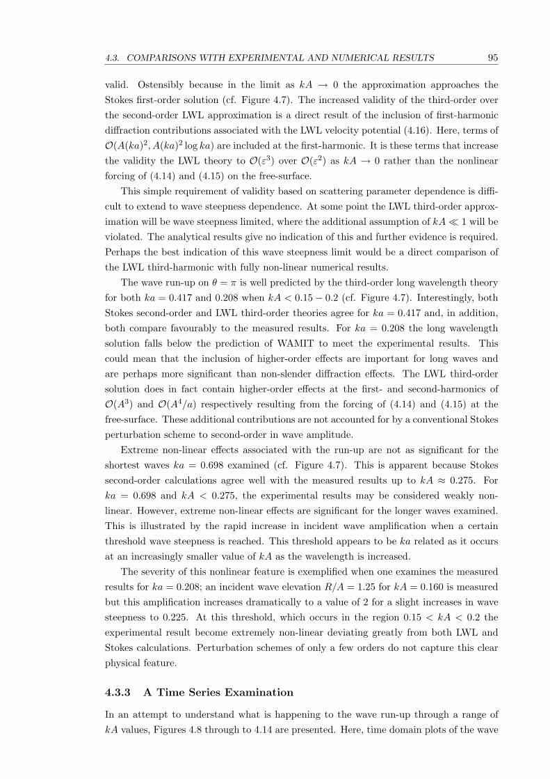
4.3. COMPARISONS WITH EXPERIMENTAL AND NUMERICAL RESULTS 95
valid. Ostensibly because in the limit as kA → 0 the approximation approaches theStokes first-order solution (cf. Figure 4.7). The increased validity of the third-order overthe second-order LWL approximation is a direct result of the inclusion of first-harmonicdiffraction contributions associated with the LWL velocity potential (4.16). Here, terms ofO(A(ka)2, A(ka)2 log ka) are included at the first-harmonic. It is these terms that increasethe validity the LWL theory to O(ε3) over O(ε2) as kA → 0 rather than the nonlinearforcing of (4.14) and (4.15) on the free-surface.
This simple requirement of validity based on scattering parameter dependence is diffi-cult to extend to wave steepness dependence. At some point the LWL third-order approx-imation will be wave steepness limited, where the additional assumption of kA ¿ 1 will beviolated. The analytical results give no indication of this and further evidence is required.Perhaps the best indication of this wave steepness limit would be a direct comparison ofthe LWL third-harmonic with fully non-linear numerical results.
The wave run-up on θ = π is well predicted by the third-order long wavelength theoryfor both ka = 0.417 and 0.208 when kA < 0.15− 0.2 (cf. Figure 4.7). Interestingly, bothStokes second-order and LWL third-order theories agree for ka = 0.417 and, in addition,both compare favourably to the measured results. For ka = 0.208 the long wavelengthsolution falls below the prediction of WAMIT to meet the experimental results. Thiscould mean that the inclusion of higher-order effects are important for long waves andare perhaps more significant than non-slender diffraction effects. The LWL third-ordersolution does in fact contain higher-order effects at the first- and second-harmonics ofO(A3) and O(A4/a) respectively resulting from the forcing of (4.14) and (4.15) at thefree-surface. These additional contributions are not accounted for by a conventional Stokesperturbation scheme to second-order in wave amplitude.
Extreme non-linear effects associated with the run-up are not as significant for theshortest waves ka = 0.698 examined (cf. Figure 4.7). This is apparent because Stokessecond-order calculations agree well with the measured results up to kA ≈ 0.275. Forka = 0.698 and kA < 0.275, the experimental results may be considered weakly non-linear. However, extreme non-linear effects are significant for the longer waves examined.This is illustrated by the rapid increase in incident wave amplification when a certainthreshold wave steepness is reached. This threshold appears to be ka related as it occursat an increasingly smaller value of kA as the wavelength is increased.
The severity of this nonlinear feature is exemplified when one examines the measuredresults for ka = 0.208; an incident wave elevation R/A = 1.25 for kA = 0.160 is measuredbut this amplification increases dramatically to a value of 2 for a slight increases in wavesteepness to 0.225. At this threshold, which occurs in the region 0.15 < kA < 0.2 theexperimental result become extremely non-linear deviating greatly from both LWL andStokes calculations. Perturbation schemes of only a few orders do not capture this clearphysical feature.
4.3.3 A Time Series Examination
In an attempt to understand what is happening to the wave run-up through a range ofkA values, Figures 4.8 through to 4.14 are presented. Here, time domain plots of the wave

96 CHAPTER 4. LONG WAVELENGTH APPROXIMATION
run-up are examined for ka = 0.208 and seven different wave steepness values ranging fromkA = 0.055−0.233. The figures include the reconstructed measured values of the wave run-up from first-, second- and third-harmonics. Also included, is the WAMIT second-orderand third-order LWL predictions. For all measured and calculated time series’ the meancomponent is removed and the phase of the third-order LWL approximation is correctedby π/2. Moreover, to assist in examining the local maxima, the wave run-up peaks havebeen extracted from each of these plots and are enlarged in Figure 4.15.
The removal of the mean component reveals that largely all of the wave run-up isaccounted for by time varying contributions in waves of small to moderate wave steepness.However, once the wave steepness increases beyond the range of 0.15 < kA < 0.2 the meancomponent contribution is quite significant accounting for approximately 20% of the run-up when kA = 0.231 (cf. Figure 4.7 and Figure 4.15). The results presented in Chapter3 suggested that this mean component is significantly under predicted by perturbationschemes to second-order in kA. Therefore, it is prudent to analyse the results with thezero-harmonic removed.
At wave steepnesses below the aforementioned threshold, 0.15 < kA < 0.2, we cansee that the third-harmonic contribution reduces actual wave run-up. In contrast, thewave run-up above this threshold is increased by the third-harmonic contribution (cf.Figure 4.15). This effect can only be attributed to phase differences and implies that thephase of the third-harmonic varies with wave steepness. This effect is perhaps the reasonwhy Buchmann (1996); Buchmann et al. (2000) observed that the inclusion of third-orderdiffraction terms to a second-order model significantly improves correspondence with fullynon-linear computations of free-surface elevations both with and without the presence ofa bluff body in the fluid domain in small kA.
With the mean component of the wave run-up removed we can see that the LWLthird-order theory reasonably predicts the amplitude of the time varying portion of thewave run-up in waves of small to moderate steepness. This is particularly evident for(ka, kA) = (0.208, 0.055), (0.208, 0.152) and (0.208, 0.160), where the third-order LWLtheory performs better than the Stokes second-order calculations. However, for wavesteepnesses greater than kA ≈ 0.2, severe non-linearities occur in the second-harmonic toan extent where both Stokes second-order and LWL third-order predictions are deficient.This is particularly evident for kA = 0.231 (cf. Figure 4.15). This observation impliesthat both non-slender and higher-order diffraction effects are very significant contributorsto the second-harmonic wave run-up in waves of large kA.
This extreme non-linear feature of the measured wave run-up is not captured by po-tential flow calculations based on either Stokes perturbation to second-order or third-orderlong wavelength theory. This is perhaps the most significant reason why wave run-up pre-dictions must be based on completely non-linear methods where the governing free-surfaceboundary condition (4.11) is solved exactly. However, to the authors knowledge there areno commercially available fully non-linear potential flow codes for wave-structure interac-tion, whilst those that have been presented (see Ferrant et al., 1999; Liu et al., 2001; Xueet al., 2001, for instance) have not been sufficiently validated with experimental resultsconcerning wave run-up. Until this situation is remedied one must rely upon empirical

4.3. COMPARISONS WITH EXPERIMENTAL AND NUMERICAL RESULTS 97
0 0.5 1 1.5 2 2.5 3
−1
−0.5
0
0.5
1
1.5
t / T
R /
A
ka = 0.208, kA = 0.234
Figure 4.8: The normalised wave run-up for a truncated circular cylinder plotted against nor-malised time t/T . The mean component from both measured and calculated values is removed.Reconstructed measured wave run-up to the third-harmonic (—–); Reconstructed measured waverun-up to the second-harmonic (· · · ); second-order WAMIT (– · –); and third-order long wavelength(– – –).
methods, with some rational basis, to account for the extreme non-linearity of the waverun-up in steep waves (kA > 0.15− 0.2) of moderate to long wavelength.
4.3.4 The Wave Run-up for Arbitrary θ
We now turn our attention to the free-surface elevation around the boundary of the circularcylinder. Figures 4.16, 4.17 and 4.18 show the maximum wave crest amplification arounda truncated circular cylinder D/a = 2.53 calculated from LWL second- and third-ordertheory. In addition, both first- and second-order Stokes perturbation predictions (fromWAMIT) and experimental results are shown. The comparison is for ka = 0.208 (cf.Figure 4.16), ka = 0.417 (cf. Figure 4.17) and ka = 0.698 (cf. Figure 4.18) for a range ofcombinations (ka, kA). The results for ka = 0.283 are not expected to be valid because ofpossible wave tank resonant excitation and are therefore not shown.
Apart from waves of small steepness, the LWL formulation severely under predictsthe measured wave run-ups at θ/π = 0.5 and 0.75 for all combinations of (ka, kA). Thisunder prediction is caused by dominate cos θ symmetry terms associated with the second-harmonic contributions from ζ(3) which are of incorrect phasing. The combinations of(ka, kA) = (0.208, 0.055) and (0.417, 0.057) are the only instances where the LWL for-mulation appears to predict the measured wave amplification at the three positions of θ
considered.In contrast, the second-order perturbation theory predictions compare much better
to measured values at θ/π = 0.5 and 0.75 and shows the minimum wave run-up to bein the region 0 < θ/π < 0.5. This local minima is caused through an increase in fluidmomentum as the flow negotiates the cylinder, hence to conserve energy, the free-surface

98 CHAPTER 4. LONG WAVELENGTH APPROXIMATION
0 0.5 1 1.5 2 2.5 3
−1
−0.5
0
0.5
1
1.5
t / T
R /
A
ka = 0.208, kA = 0.231
Figure 4.9: The normalised wave run-up for a truncated circular cylinder plotted against nor-malised time t/T . The mean component from both measured and calculated values is removed.Reconstructed measured wave run-up to the third-harmonic (—–); Reconstructed measured waverun-up to the second-harmonic (· · · ); second-order WAMIT (– · –); and third-order long wavelength(– – –).
0 0.5 1 1.5 2 2.5 3
−1
−0.5
0
0.5
1
1.5
t / T
R /
A
ka = 0.208, kA = 0.2
Figure 4.10: The normalised wave run-up for a truncated circular cylinder plotted against nor-malised time t/T . The mean component from both measured and calculated values is removed.Reconstructed measured wave run-up to the third-harmonic (—–); Reconstructed measured waverun-up to the second-harmonic (· · · ); second-order WAMIT (– · –); and third-order long wavelength(– – –).
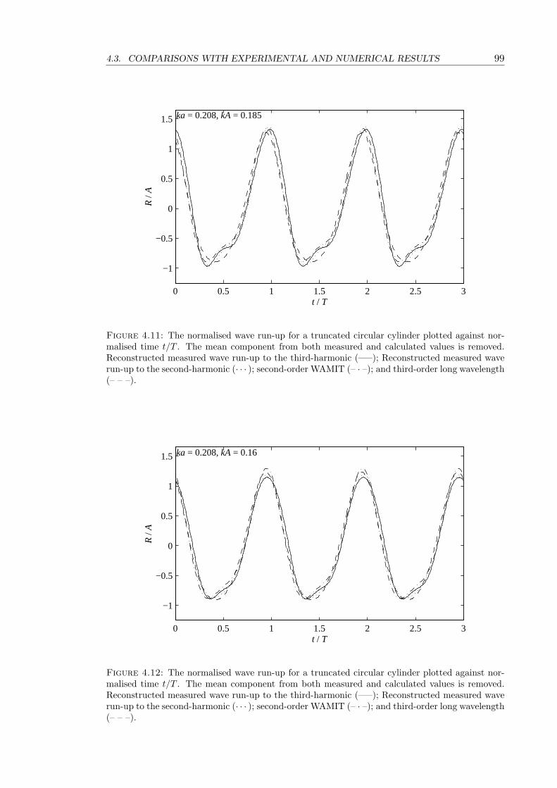
4.3. COMPARISONS WITH EXPERIMENTAL AND NUMERICAL RESULTS 99
0 0.5 1 1.5 2 2.5 3
−1
−0.5
0
0.5
1
1.5
t / T
R /
A
ka = 0.208, kA = 0.185
Figure 4.11: The normalised wave run-up for a truncated circular cylinder plotted against nor-malised time t/T . The mean component from both measured and calculated values is removed.Reconstructed measured wave run-up to the third-harmonic (—–); Reconstructed measured waverun-up to the second-harmonic (· · · ); second-order WAMIT (– · –); and third-order long wavelength(– – –).
0 0.5 1 1.5 2 2.5 3
−1
−0.5
0
0.5
1
1.5
t / T
R /
A
ka = 0.208, kA = 0.16
Figure 4.12: The normalised wave run-up for a truncated circular cylinder plotted against nor-malised time t/T . The mean component from both measured and calculated values is removed.Reconstructed measured wave run-up to the third-harmonic (—–); Reconstructed measured waverun-up to the second-harmonic (· · · ); second-order WAMIT (– · –); and third-order long wavelength(– – –).

100 CHAPTER 4. LONG WAVELENGTH APPROXIMATION
0 0.5 1 1.5 2 2.5 3
−1
−0.5
0
0.5
1
1.5
t / T
R /
A
ka = 0.208, kA = 0.152
Figure 4.13: The normalised wave run-up for a truncated circular cylinder plotted against nor-malised time t/T . The mean component from both measured and calculated values is removed.Reconstructed measured wave run-up to the third-harmonic (—–); Reconstructed measured waverun-up to the second-harmonic (· · · ); second-order WAMIT (– · –); and third-order long wavelength(– – –).
0 0.5 1 1.5 2 2.5 3
−1
−0.5
0
0.5
1
1.5
t / T
R /
A
ka = 0.208, kA = 0.055
Figure 4.14: The normalised wave run-up for a truncated circular cylinder plotted against nor-malised time t/T . The mean component from both measured and calculated values is removed.Reconstructed measured wave run-up to the third-harmonic (—–); Reconstructed measured waverun-up to the second-harmonic (· · · ); second-order WAMIT (– · –); and third-order long wavelength(– – –).

4.3. COMPARISONS WITH EXPERIMENTAL AND NUMERICAL RESULTS 101
1.8 1.9 2 2.1
1
1.2
1.4
1.6
t / T
R /
A
ka = 0.208, kA = 0.231
1.8 1.9 2 2.1
1
1.2
1.4
1.6
t / T
R /
A
ka = 0.208, kA = 0.2
1.8 1.9 2 2.1
1
1.2
1.4
1.6
t / T
R /
A
ka = 0.208, kA = 0.185
1.8 1.9 2 2.1
1
1.2
1.4
1.6
t / T
R /
A
ka = 0.208, kA = 0.16
1.8 1.9 2 2.1
1
1.2
1.4
1.6
t / T
R /
A
ka = 0.208, kA = 0.152
1.8 1.9 2 2.1
1
1.2
1.4
1.6
t / T
R /
A
ka = 0.208, kA = 0.055
Figure 4.15: The magnified normalised wave run-up for one particular crest extracted fromFigures 4.9-4.14. The mean component from both measured and calculated values is removed.Reconstructed measured wave run-up to the third-harmonic (—–); Reconstructed measured waverun-up to the second-harmonic (· · · ); second-order WAMIT (– · –); and third-order long wavelength(– – –).

102 CHAPTER 4. LONG WAVELENGTH APPROXIMATION
must decrease in elevation accordingly. It is worth noting that the exact position of thislocal minima appears to be both a function of ka and kA. As expected, the position ofthis minima moves closer to θ/π = 0.5 in the limit of ka → 0. This is due to the cylinderbecoming increasingly transparent as the incident wavelength increases. The influenceof wave steepness tends to shift the minimum run-up towards θ/π = 0 for increasingkA. Furthermore, this minimum appears to decrease with a subsequent increase in kA
of around 30% between kA = 0.055 and 0.231 (see Figure 4.16). This decrease is moreprominent for ka = 0.208 than the shorter waves of ka = 0.417 and ka = 0.698.
Of the three scattering parameters examined, Stokes second-order diffraction predic-tions show the most favourable agreement with the wave run-up around the cylinder forka = 0.698 (see Figure 4.18). The agreement here is perhaps better for smaller kA buteven for large kA the agreement is still quite reasonable. For ka = 0.698, previous discus-sions have suggested that the measured wave run-up for increasing kA is best predicted byStokes second-order diffraction theory (cf. Figure 4.7). The comparison shown in Figure4.18, for ka = 0.698, agrees with this observation and goes further to suggest that thewave run-up around the cylinder surface is the result of weakly non-linear effects only andtherefore it is sufficiently accounted for by second-order diffraction theory.
4.3.5 Computational Remarks
Provided the assumptions of ka ¿ 1, kA ¿ 1 and A/a = O(1) are not violated the third-order long wavelength theory performs well against the complete second-order diffractionsolution, the solution of which is easily programmable and computation times are ex-tremely efficient. This is in stark contrast to the BEM, used for the second-order diffrac-tion problem, where accurate computations of the free-surface elevation for one particularwave frequency can take up to 90 minutes on a Pentium II 650Mhz PC with fine body andfree-surface meshing schemes. Given that a BEM method computation requires extensiveconvergence studies for reliable results, and the free-surface elevation to second-order iscomputationally expensive, the simplified method presented here offers an efficient alter-native.
4.4 Chapter Summary
A long wavelength theory for the free-surface elevation to O(ε3), where the exact free-surface boundary condition has been treated by an expansion in terms of ε1 = kA and ε2 =ka, has been presented. The wave run-up comprising the first few harmonic componentscan be evaluated efficiently provided that the intrinsic assumptions of A/a = O(1), ka ¿ 1and kA ¿ 1 are not violated. Comparisons with measured results suggest that the LWLprediction of the wave run-up to third-order is reasonable for small values of ka belowa certain threshold wave steepness 0.15 < kA < 0.2. Beyond this threshold both thelong wavelength approximation and the Stokes second-order prediction of the wave run-up become deficient. It is thought that this deficiency is mainly caused by higher-orderdiffraction effects that operate at the second-harmonic of the wave run-up. In addition, afurther discrepancy is also thought to be associated with a mean set-up which is developed

4.4. CHAPTER SUMMARY 103
on the up-wave side of the cylinder. The cause of this mean set-up is unclear. Stokesperturbation and hence long wavelength assumptions fail to capture the physics associatedwith this mean set-up. Given the computational burden required to evaluate the free-surface elevation and wave run-up around a cylinder with boundary element methods,simplified methods provide an attractive avenue for continued investigation.

104 CHAPTER 4. LONG WAVELENGTH APPROXIMATION
0 0.5 10
0.5
1
1.5
2
θ / π
R(θ
) / A
ka = 0.208, kA = 0.231
0 0.5 10
0.5
1
1.5
2
θ / π
R(θ
) / A
ka = 0.208, kA = 0.2
0 0.5 10
0.5
1
1.5
2
θ / π
R(θ
) / A
ka = 0.208, kA = 0.185
0 0.5 10
0.5
1
1.5
2
θ / π
R(θ
) / A
ka = 0.208, kA = 0.16
0 0.5 10
0.5
1
1.5
2
θ / π
R(θ
) / A
ka = 0.208, kA = 0.152
0 0.5 10
0.5
1
1.5
2
θ / π
R(θ
) / A
ka = 0.208, kA = 0.055
Figure 4.16: The maximum wave run-up around a truncated vertical cylinder (D/a = 2.53)in monochromatic incident waves with ka = 0.208. Measured vs. calculated values. Measuredresults (•); third-order long wavelength theory (—–); second-order long wavelength theory (· · · );second-order diffraction (– – –); and linear theory (– · –).

4.4. CHAPTER SUMMARY 105
0 0.5 10
0.5
1
1.5
2
θ / π
R(θ
) / A
ka = 0.417, kA = 0.244
0 0.5 10
0.5
1
1.5
2
θ / π
R(θ
) / A
ka = 0.417, kA = 0.213
0 0.5 10
0.5
1
1.5
2
θ / π
R(θ
) / A
ka = 0.417, kA = 0.2
0 0.5 10
0.5
1
1.5
2
θ / π
R(θ
) / A
ka = 0.417, kA = 0.166
0 0.5 10
0.5
1
1.5
2
θ / π
R(θ
) / A
ka = 0.417, kA = 0.156
0 0.5 10
0.5
1
1.5
2
θ / π
R(θ
) / A
ka = 0.417, kA = 0.057
Figure 4.17: The maximum wave run-up around a truncated vertical cylinder (D/a = 2.53)in monochromatic incident waves with ka = 0.417. Measured vs. calculated values. Measuredresults (•); third-order long wavelength theory (—–); second-order long wavelength theory (· · · );second-order diffraction (– – –); and linear theory (– · –).

4.1. LONG WAVELENGTH THEORY 71
incident wavelength is asymptotically large when compared to the column radius. Whilethe restriction placed on A/a implies that the wave amplitude is of the same order ofmagnitude as the column radius. In Faltinsen et al. (1995), the wave force to third-orderin wave amplitude, O(A3), is derived on these long wavelength assumptions.
Results from Krokstad & Stansberg (1995), illustrate that FNV theory significantlyover predicts the second-order force components when compared to model experiments.This would suggests that the second-order force is clearly influenced by non-slender far fielddiffraction effects. However, Krokstad & Stansberg (1995) also demonstrate a reasonableagreement for third-order force components between the theory of FNV and experiments.To reconcile this, Krokstad & Stansberg (1995) suggest that non-slender far field diffractioneffects exhibit a lesser bearing on the third-order than second-order force. Based on thiswork, Solaas & Krokstad (2000) implemented the third-harmonic wave loads from FNVinto the time domain impulse response code ‘SIMO’ for an improved perturbation basedringing model.
The long wavelength approach of FNV has been generalised by Newman (1996a) for thecase of unidirectional irregular waves, where the wavelength of each spectral component isassumed large compared to the cylinder radius. FNV theory has been further generalisedby Faltinsen (1995, 1999) for the third-harmonic force associated with general cylindercross-sections using slender body approximations and conformal mapping through Lewisforms. In so far as the free-surface elevation is concerned, Newman & Lee (1995) pre-sented a comparison of the FNV second-order free-surface elevation with complete Stokessecond-order numerical results from WAMIT. This comparison demonstrated a reasonableagreement of the two methods for small values of ka at θ/π = 1.
Experimental evidence obtained within this study suggests that for wave run-up, in-termediate to long wavelengths are indeed critical. Furthermore, the amplitudes of thesewaves are of comparable magnitude to the column radius. In this long wavelength regime,third-harmonic components of the wave run-up become important. Moreover, non-lineareffects operating at the first-harmonic were clearly observed for increasing values of wavesteepness. Such effects can be included in the prediction of wave run-up through a per-turbation scheme accounting for wave amplitude dependent terms of O(A3).
With a consistent perturbation expansion based on kA = O(ε), ka = O(ε) and A/a =O(1), the work presented here extends the LWL theory of FNV to account for the free-surface elevation correct to O(ε3) for regular waves of amplitude A incident upon a fixedvertical surface piercing cylinder of radius a. In doing so, higher-order terms of the free-surface elevation proportional to A3 and A4/a are found. These terms operate at both thefirst- and third-harmonics for A3 and the mean-, second-, and fourth-harmonics for A4/a.
The resulting equations are derived in a somewhat different manner than that consid-ered in FNV. In this work, greater understanding is achieved by considering two perturba-tion schemes that correspond to an expansion in terms of the wave steepness and cylinderslenderness parameters. As a consequence, a connection is made with the experimentalwork considered in §2.1.
In the solution procedure, the classical linear diffraction potential for a circular cylinderin monochromatic waves is revisited in §4.1.1. However, the appropriate expansion for long
106 CHAPTER 4. LONG WAVELENGTH APPROXIMATION
0 0.5 10
0.5
1
1.5
2
θ / π
R(θ
) / A
ka = 0.698, kA = 0.261
0 0.5 10
0.5
1
1.5
2
θ / π
R(θ
) / A
ka = 0.698, kA = 0.233
0 0.5 10
0.5
1
1.5
2
θ / π
R(θ
) / A
ka = 0.698, kA = 0.212
0 0.5 10
0.5
1
1.5
2
θ / π
R(θ
) / A
ka = 0.698, kA = 0.179
0 0.5 10
0.5
1
1.5
2
θ / π
R(θ
) / A
ka = 0.698, kA = 0.162
0 0.5 10
0.5
1
1.5
2
θ / π
R(θ
) / A
ka = 0.698, kA = 0.062
Figure 4.18: The maximum wave run-up around a truncated vertical cylinder (D/a = 2.53)in monochromatic incident waves with ka = 0.698. Measured vs. calculated values. Measuredresults (•); third-order long wavelength theory (—–); second-order long wavelength theory (· · · );second-order diffraction (– – –); and linear theory (– · –).

Chapter 5
Parametric Study on Column
Geometry
Presently, the work of Nielsen (2000), reviewed in §2.2, is the only instance where the waverun-up on a square cylinder with rounded edges has been investigated. For the purposeof this thesis, the geometry of a rounded edge is described by the ratio rc/a. In Nielsen(2000), only two values of this ratio were considered, namely rc/a = 1 corresponding to acircular cylinder and rc/a = 0.5 for an intermittently square cylinder. Moreover, wave run-up on a completely square cylinder, where rc/a = 0, has yet to be studied. Subsequently,there is a limited amount of published data available to platform designers on the extentto which the parameter rc/a affects the wave run-up on a vertical cylinder. The purposeof this chapter is to partially rectify this situation by studying a broad range of normalisedcorner radius values, in particular, within the domain 0 ≤ rc/a ≤ 1. The experimentalmeasurements for this investigation were introduced in Chapter 2.
Firstly, a numerical study using potential flow results from WAMIT will be shownin §5.1 to illustrate the effect of rc/a on the mean, first-, and second-order wave run-up components. The effect of rc/a on the harmonic contributions to the wave run-upis discussed in §5.2. To assist platform designers in predicting the effect of rc/a on thewave run-up a simplified model is suggested in §5.3. This simplified model incorporatesboth geometry and diffraction effects to first-order in wave amplitude plus additionalhigher-order diffraction effects for long wavelengths. Finally, with the aid of experimentalresults, the limitations of this simplified wave run-up model, along with Stokes second-order diffraction results, are discussed in §5.4.
5.1 Numerical Study of Cross-Section Effects
To investigate the influence of a variation in rc/a on the wave run-up on a cylindricalcolumn, the boundary element method program WAMIT was first used. In particular, thefive truncated vertical surface piercing cylinders, discussed in the experimental campaign,were considered in the numerically modelling. We recall that D/a = 2.53 and the cornerradius variation for the five cylinders corresponds to rc/a = 0, 0.25, 0.5, 0.75 and 1. Thecircular cylinder is depicted by rc/a = 1 and the square by rc/a = 0. The restriction is

108 CHAPTER 5. PARAMETRIC STUDY ON COLUMN GEOMETRY
again made to monochromatic incident waves of small amplitude such that A ¿ L. Thefree-surface elevations and wave run-up calculations around the surface of each cylinderwere obtained to first- and second-order using WAMIT.
5.1.1 A Note on the Square Cylinder
It is worth noting that the assumption of irrotational flow in the presence of bodies withdiscontinuous surfaces or sudden tangent changes is, strictly speaking, invalid over theentire fluid domain. Nevertheless, if eddy formation resulting from fluid interaction withthe rounded edges of the square cylinders is assumed localised, and consequently convecteddownstream along with the incident flow, then the assumption of irrotational solenoidalflow may indeed be justified along the ray θ = π. This assumption would of course becomeinvalid when the body’s cross-sectional geometry gives A/a > O(1). However, we are onlyconcerned with large volume structures and the ray of θ = π is of particular importanceto the maximum wave run-up experienced by each cylinder.
It should also be pointed out that an assumption of an irrotational fluid domain inthe neighbourhood a square cylinder, rc/a = 0, will be invalid. This is best pointedout if steady inviscid incident flow is considered around two stationary plane boundariesextending to infinity and intersecting with an included angle of θ = π/2, as depicted inFigure 5.1. The origin is taken as the intersection of these two planes, and with zero-flux boundary conditions applied at θ = 0 and 3π/2, the solution to the BVP yields thefollowing velocity potential for external flow
φ = Ar2/3 cos23θ, (5.1)
where A is a real constant. From (5.1) it can be shown that the fluid velocity becomessingular as r → 0. This analogy and hence the velocity potential given by (5.1) will holdin the immediate neighbourhood of the square cylinder in the absence of oscillatory flow(or alternatively as ka → 0). This is of course not physical and results directly from theassumption of irrotational flow. In reality, the fluid separates at this discontinuity (seeBatchelor, 1967, pages 410-413).
To alleviate this problem in the potential flow model, particular attention was paid tothe meshing scheme used in the vicinity of discontinuities and rounded edges of the squarecylinders. As suggested by Faltinsen (1990), a very fine mesh was employed around areaswith sudden tangent changes to obtain meaningful numerical results at θ/π = 1. In spiteof this measure, the fluid velocity remains infinite in the potential flow model for thesquare cylinder in the vicinity of each corner.
5.1.2 Numerical Results
As a preliminary, a convergence analysis of the second-order 2ω free-surface elevationwas performed. The abbreviated results of this study for rc/a = 0 at (r, θ) = (a, π) arepresented in Table 5.1. This particular case is important in view of the discussion outlinedin §5.1.1, and hence, it is equally desirable to illustrate sufficient accuracy of the numericalresults. It is clearly shown that three and four significant figure accuracy is obtained for

5.1. NUMERICAL STUDY OF CROSS-SECTION EFFECTS 109
Zero Flux Boundaries
Streamlines
Figure 5.1: Streamlines of irrotational flow around a corner formed by zero flux boundaries ofincluded angle π/2.
small and large values of ka respectively.Although not shown here, a similar convergence analysis was carried out for the first-
and second-order free-surface elevations for each rc/a and ka combination with excellentresults. For each cylinder 1500 to 12000 panels on Sb were considered. Generally, 1500body panels were sufficient for accurate first-order calculations of each cylinder. For thesecond-order analysis, a selection of free-surface panels ranging from 12000 to 30000 werechosen. Due to large velocity gradients at the intersection of the body and free-surface,these panels were organised such that the characteristic dimensions of each panel system-atically decreased at the approach of this intersection along both Sf and Sb. Furthermore,a numerical study on the position of the partition radius for the inner domain on Sf sug-gested that a value of 20m from the Sb produced the best results for the shortest waveperiods.
The normalised numerical results, of the free-surface elevation on a truncated surfacepiercing cylinder, are given in Figures 5.2, 5.3 and 5.4. These figures correspond to thefirst-order, second-order second-harmonic and second-order mean components respectively.The results pertain to the maximum wave run-up position at r = a and θ = π.
The influence of rc/a variation on the modulus of the first-order free-surface elevationis clearly visible (see Figure 5.2). The first-order free-surface elevation demonstrates asystematic increase in amplification as rc/a decreases from 1 to 0 (i.e. the evolution froma circular to square cylinder). As rc/a → 0 a distinct amplification of ζ(1) is observedin the range of 1 < ka < 2. This amplification is as much as 1.5 times the linear resultof Havelock (1940). The phase of these first-order numerical results appears to be lessinfluenced by the rc/a variation.
In the limit as ka becomes large, this amplification must be arrested. It is reasonableto suggest that, regardless of cylinder geometry, |ζ(1)|/A will approach a linear valueof 2 as ka → ∞. This is dictated by the method of geometric optics for a circularcylinder elucidated by Newman (1996b). In the ‘illuminated’ region on the upwave side of

110 CHAPTER 5. PARAMETRIC STUDY ON COLUMN GEOMETRY
Table 5.1: The results of a convergence study on the second-order wave elevation for a truncatedvertical cylinder, rc/a = 0. The rows of each ka value correspond to 6400 and 12000 body panelsrespectively. The columns from left to right correspond to 22400, 28800, 10800, 18000, 24000and 30000 free-surface panels respectively. The partition radius columns 1,2 and 20m while forremaining columns 15m was used.
ka Second-order free-surface elevation1.3858 0.31814 0.31653 0.32307 0.32252 0.32088 0.32001
0.33531 0.33349 0.33191 0.32852 0.32655 0.32602
0.6979 0.11709 0.11751 0.11742 0.11724 0.11698 0.117040.11709 0.11753 0.11837 0.11891 0.11873 0.11870
0.4167 0.06876 0.06881 0.06876 0.06868 0.06860 0.068650.06875 0.06886 0.06893 0.06894 0.06887 0.06890
0.2826 0.07125 0.07126 0.07125 0.07120 0.07116 0.071200.07139 0.07145 0.07143 0.07140 0.07136 0.07139
0.2077 0.05089 0.05088 0.05088 0.05087 0.05086 0.050860.05097 0.05098 0.05093 0.05090 0.05090 0.05090
the cylinder the first-order potential φ(1) consists of both an incident and reflected wavecomponent with the same amplitude and phase on the cylinder given by
φ(1) = i2gA/ωekz−ika cos θ for π/2 < θ < 3π/2, (5.2)
from which, it is easy to deduce that the maximum wave amplification in the short wave-length limit is 2A. Regardless of cylinder geometry, this limit will always result. The formof (5.2) is essentially the cylindrical domain equivalent to the infinitely long vertical wallcase (cf. §3.2). The phase of ζ(1) in this limit must be such that a standing wave resultsin front of the cylinder.
It is also worth noting that the numerical results of Figure 5.2 indicate that leadingorder local diffraction effects in the limit as ka → 0 also approach the linear diffractionsolution of Havelock (1940). Intuitively one would expect this result since the cylinderwould become increasingly transparent to the onset oscillatory flow as the wavelengthincreases. It is therefore reasonable to expect that, regardless of rc/a, as ka → (0,∞), thelinear diffraction result of Havelock (1940) is approached. In other words, incident waveamplifications of ζ(1)/A = 1 and 2 for ka → 0 and ∞ respectively at r = a.
Attention is now turned to the corresponding numerical results for the second-ordersecond-harmonic free-surface elevation (cf. Figure 5.3) at (r, θ) = (a, π). In contrast tothe first-harmonic, it is obvious that the second-order 2ω component does not show asystematic increase in magnitude as rc/a → 0. For instance, when ka < 0.3 the leadingorder second-harmonic does not appear to be affected by rc/a. However, when ka ≈ 0.3 areversal in the magnitude of local wave diffraction is noted, whereby ζ(2) for the circularcylinder is greater than that of the square cross-section. The reason for this is unclear.Nevertheless, once ka values fall within the domain 0.4 < ka < 1 the numerical resultsappear as expected, whereby rc/a = 0 produces the greatest amplification effect on ζ(2)
and that of rc/a = 1 gives the least. All intermediate values of rc/a subsequently follow

5.1. NUMERICAL STUDY OF CROSS-SECTION EFFECTS 111
0 0.5 1 1.5 21
1.5
2
2.5
3
ka
| ζ(1
) | / A
0 0.5 1 1.5 20
0.1
0.2
0.3
0.4
0.5
0.6
0.7
0.8
ka
θ(1) /
π
Figure 5.2: The affect of corner radius variation on the normalised first-order first-harmonic free-surface elevation at (r, θ) = (a, π) for a vertical truncated surface piercing cylinder D/a = 2.53.The left and right plots show the modulus and phase respectively. Five different rc/a values areshown: circular cylinder rc/a = 1, a solid line with (•); rc/a = 0.75, (– · –); rc/a = 0.5, (– – –);rc/a = 0.25, (· · · ); square cylinder rc/a = 0, (——).
systematically in between these two limits.However, for values of ka > 1 the second-harmonic again follows an unsystematic trend
due to wave diffraction around the corners of the square cylinders. This is particularlyevident for rc/a = 0.75 and 0.5 where the amplification of ζ(2) is actually less than thatfor rc/a = 1. The physical reasons for this unexpected local diffraction effect are unclear.Moreover, this is not thought to be caused by numerical error as great care was observedduring the convergence studies of the second-order results in the range of 0 < ka < 2.At the upper end of ka > 1.5 some difficultly was encountered, and in some cases only 2significant figure convergence could be achieved. The numerical results were also checkedwith irregular frequencies removed from the calculations (see Lee et al., 1996; WAMIT,1995, for details on irregular frequencies) and no apparent differences were realised.
The numerical results suggest that the phase of the second-order second-harmonicfree-surface elevation is little affected by rc/a for ka < 0.4 (cf. Figure 5.3). This resultis similar to the corresponding modulus and implies that cylinder geometry effects haveyet to significantly influence local wave diffraction. One striking observation should benoted; the numerical results indicate that for large ka when rc/a ≤ 0.5 the phase of thesecond-harmonic becomes negative. This phase difference has the effect, when added to themean- and first-harmonic components, of reducing the free-surface elevation prediction.Comparisons of the wave elevation on and in front of these cylinders with measured valuesfor ka = 1.386 will indicate that this is not physically occurring and shall be shown later.
The second-order mean component, unlike its second-harmonic counterpart, behavesin a very systematic manner when influenced by a systematic variation of rc/a. This isbest illustrated in Figure 5.4. It is shown that local diffraction, associated with the changein rc/a from 1 to 0, is not significantly affected for ka < 1. However, for values of ka > 1,local diffraction effects associated with rc/a become increasingly significant and greatly

112 CHAPTER 5. PARAMETRIC STUDY ON COLUMN GEOMETRY
0 0.5 1 1.5 20
0.5
1
1.5
2
2.5
3
3.5
ka
| ζ(2
) | a
/ A2
0 0.5 1 1.5 2−1.5
−1
−0.5
0
0.5
1
1.5
kaθ(2
) / π
Figure 5.3: The affect of corner radius variation on the normalised second-order second-harmonicfree-surface elevation at (r, θ) = (a, π) for a vertical truncated surface piercing cylinder D/a = 2.53.The left and right plots show the modulus and phase respectively. Five different rc/a values areshown: circular cylinder rc/a = 1, a solid line with (•); rc/a = 0.75, (– · –); rc/a = 0.5, (– – –);rc/a = 0.25, (· · · ); square cylinder rc/a = 0, (——).
enhance the mean set-up. This mean set-up systematically increases as rc/a → 0. In thelimit as ka becomes large, regardless of rc/a, it is expected that the mean componentwill reduce to the related problem of the wave reflection by an infinitely long vertical wall,where to second-order the mean free-surface elevation is given by ζ = kA2 cos kx (cf. §3.2).
5.2 Influence of Geometry on the Harmonic Components
Before examining the actual measured wave run-up, important information can first begained by examining the harmonic contributions to it. An understanding of how wellthese Fourier modes, under the influence of an rc/a variation, are predicted by a second-order in Stokes expansion potential flow model will assist in identifying and explainingdiscrepancies in the actual wave run-up. For the purpose of this investigation, we shallrestrict ourselves to four of the five scattering parameters, ka = 0.208, 0.283, 0.417 and0.698, and discard results pertaining to ka = 1.39 as these show much harmonic variabilitybecause of the inherently short wavelength.
As a preliminary, a comparison of numerical predictions and measured results is pre-sented in Figures 5.5, 5.6 and 5.7. Each of these plots correspond to the measured zero-,first- and second-harmonics and their corresponding numerical predictions respectively.The important aspect from this representation of the results is that, for each value of ka,all corresponding rc/a values are illustrated as a whole.
This comparison shows that the effect of corner radius on each harmonic appears to bemore significant for large values of ka. This is best illustrated in Figures 5.5 and 5.6 forka = 0.698. In particular, as ka increases the numerical results suggest a greater influencefrom the parameter rc/a on each of the three harmonic components investigated.
However, the magnitude of this increase with increasing ka is not replicated in the

5.2. INFLUENCE OF GEOMETRY ON THE HARMONIC COMPONENTS 113
0 0.5 1 1.5 20
0.5
1
1.5
2
2.5
3
3.5
ka
| ζ(0
) | a
/ A2
Figure 5.4: The affect of corner radius variation on the normalised second-order mean free-surface elevation at (r, θ) = (a, π) for a vertical truncated surface piercing cylinder D/a = 2.53.Five different rc/a values are shown: circular cylinder rc/a = 1, a solid line with (•); rc/a = 0.75,(– · –); rc/a = 0.5, (– – –); rc/a = 0.25, (· · · ); square cylinder rc/a = 0, (——).
measured results. The second-harmonic of the comparison aptly illustrates this discrep-ancy (cf. Figure 5.7). Moreover, the second-harmonic for a value of ka = 0.698 does notappear to be greatly influenced by rc/a at all. This discrepancy is such that the measuredsecond-harmonic for each value of rc/a appears best predicted by the numerical resultsfor rc/a = 1 alone.
The advantage of representing the data in this manner is that non-linear aspects thatwere noted for the circular cylinder (cf. §3.6) are verified. This is particularly evidentfor the first-harmonic when ka = 0.208 (cf. Figure 5.6). Here, it is clearly shown thatnon-linear effects operating at the first harmonic are important for large wave steepnesses.Despite the variation of rc/a, the precision of the measured results provides clear evidenceof this non-linearity at large kA.
Due to these non-linear effects, in the region of small ka and large kA, the first-harmonic is not well predicted by the first-order numerical results. On the contrary though,the first-harmonic is well predicted for small kA (cf. Figure 5.6) when ka = 0.208. Thisstate of affairs for general rc/a agrees with the results of §3.6. However, the small band-width of both the measured and numerical results does not permit any direct inference asto the effect of rc/a on the first-harmonic for ka = 0.208.
With the data presented in this manner (cf. Figures 5.5-5.7), it is difficult to determinewhether the effect of rc/a on each harmonic is adequately captured by the second-order inStokes expansion potential model. This is largely because of the seemingly small variationsshown for the moduli of each harmonic in the domain 0 ≤ rc/a ≤ 1. Furthermore, thesesmall variations of |R(ωn)| are of the same order of magnitude as small fluctuations ofthe incident wave Fourier modes. Although, the overall incident wave heights may behighly repeatable, it is often difficult in model experiments to obtain entire harmonicrepeatability of the incident waveform.

114 CHAPTER 5. PARAMETRIC STUDY ON COLUMN GEOMETRY
0.05 0.075 0.1 0.125 0.15 0.175 0.2 0.225 0.25 0.275 0.30
0.4
0.8
1.2
1.6
|R(ω
0)| a
/ A2
ka = 0.698
0.05 0.075 0.1 0.125 0.15 0.175 0.2 0.225 0.25 0.275 0.30
0.4
0.8
1.2
1.6
|R(ω
0)| a
/ A2
ka = 0.417
0.05 0.075 0.1 0.125 0.15 0.175 0.2 0.225 0.25 0.275 0.30
0.4
0.8
1.2
1.6
|R(ω
0)| a
/ A2
ka = 0.283
0.05 0.075 0.1 0.125 0.15 0.175 0.2 0.225 0.25 0.275 0.30
0.4
0.8
1.2
1.6
kA
|R(ω
0)| a
/ A2
ka = 0.208
Figure 5.5: Normalised zero-harmonic modulus of wave run-up at θ = π. Measured (symbols)vs. calculated (lines) values. rc/a = 1: (•) and (——); rc/a = 0.75: (×) and (– · –)dashed dotline; rc/a = 0.5: (.) and (· · · ); rc/a = 0.25: (∗) and (– – –); and rc/a = 0: (¤) and (——). Note:The top and bottom solid lines correspond to rc/a = 0 and rc/a = 1 respectively.

5.2. INFLUENCE OF GEOMETRY ON THE HARMONIC COMPONENTS 115
0.05 0.075 0.1 0.125 0.15 0.175 0.2 0.225 0.25 0.275 0.30.4
0.8
1.2
1.6
2|R
(ω1)|
/ A ka = 0.698
0.05 0.075 0.1 0.125 0.15 0.175 0.2 0.225 0.25 0.275 0.30.4
0.8
1.2
1.6
2
|R(ω
1)| / A
ka = 0.417
0.05 0.075 0.1 0.125 0.15 0.175 0.2 0.225 0.25 0.275 0.30.4
0.8
1.2
1.6
2
|R(ω
1)| / A
ka = 0.283
0.05 0.075 0.1 0.125 0.15 0.175 0.2 0.225 0.25 0.275 0.30.4
0.8
1.2
1.6
2
kA
|R(ω
1)| / A
ka = 0.208
Figure 5.6: Normalised First-harmonic modulus of wave run-up at θ = π. Measured (symbols)vs. calculated (lines) values. rc/a = 1: (•) and (——); rc/a = 0.75: (×) and (– · –)dashed dotline; rc/a = 0.5: (.) and (· · · ); rc/a = 0.25: (∗) and (– – –); and rc/a = 0: (¤) and (——). Note:The top and bottom solid lines correspond to rc/a = 0 and rc/a = 1 respectively.

116 CHAPTER 5. PARAMETRIC STUDY ON COLUMN GEOMETRY
0.05 0.075 0.1 0.125 0.15 0.175 0.2 0.225 0.25 0.275 0.30
0.3
0.6
0.9
1.2
|R(ω
2)| a
/ A2
ka = 0.698
0.05 0.075 0.1 0.125 0.15 0.175 0.2 0.225 0.25 0.275 0.30
0.3
0.6
0.9
1.2
|R(ω
2)| a
/ A2
ka = 0.417
0.05 0.075 0.1 0.125 0.15 0.175 0.2 0.225 0.25 0.275 0.30
0.3
0.6
0.9
1.2
|R(ω
2)| a
/ A2
ka = 0.283
0.05 0.075 0.1 0.125 0.15 0.175 0.2 0.225 0.25 0.275 0.30
0.3
0.6
0.9
1.2
kA
|R(ω
2)| a
/ A2
ka = 0.208
Figure 5.7: Normalised Second-harmonic modulus of wave run-up at θ = π. Measured (symbols)vs. calculated (lines) values. rc/a = 1: (•) and (——); rc/a = 0.75: (×) and (– · –)dashed dotline; rc/a = 0.5: (.) and (· · · ); rc/a = 0.25: (∗) and (– – –); and rc/a = 0: (¤) and (——). Note:The top and bottom solid lines correspond to rc/a = 0 and rc/a = 1 respectively.
5.2. INFLUENCE OF GEOMETRY ON THE HARMONIC COMPONENTS 117
5.2.1 The Influence of Geometry on the Harmonics
In order to investigate the direct influence of rc/a on each harmonic, an alternative analysisscheme is to remove all harmonic contributions associated solely with the circular cylinderfrom those of the non-circular cylinders. This procedure partially avoids the problemsassociated with the harmonic repeatability of the diffracted wave field as it is reasonableto assume that the resulting magnification of each harmonic, when rc/a → 1, is notinfluenced by variable incident wave harmonics. Moreover, this methodology essentiallyprovides the rounded edge effect on each harmonic component of the wave run-up. Thismethodology is now applied to analyse the effect of rc/a on R(ω0), R(ω1) and R(ω2).
To illustrate the effect of rc/a on each harmonic at the position r = a and θ = π, Figures5.8, 5.9, and 5.10 are presented. These figures correspond to the first-, zero-, and second-harmonics respectively. In each figure the corresponding harmonic contributions associatedwith the circular cylinder are removed from both the measured and numerical results. Todistinguish it, the harmonics of the circular cylinder are denoted |R0(ωn)| where n = 0, 1and 2 for each harmonic studied. Furthermore, to obtain a wave steepness independentcomparison, the measured harmonics are wave steepness averaged. This provides a singlevalue of |R(ωn)| for each combination of ka and rc/a. Moreover, the experimental evidenceto support this procedure is outlined in §3.6, where the measured results for the circularcylinder indicated that each normalised harmonic remains relatively constant with wavesteepness kA. The absolute relative errors of this kA averaging procedure are presentedin Tables 5.2-5.4 and will aid in the following discussions regarding each harmonic and theeffect of rc/a.
5.2.1.1 The First-Harmonic and rc/a
The effect of this corner radius variation on the first-harmonic of the wave run-up isclearly evident in Figure 5.8. For ka = 0.698 in particular, the square cylinder exhibitsan increased wave amplification of roughly 12% over the circular cylinder case. Thisamplification is reduced as ka becomes small and monotonically decreases with rc/a. Forsmall ka the cylinder becomes increasing transparent to the onset flow and local diffractioneffects are of lesser importance than non-linearities associated with the incident wavesteepness kA. Hence, the minor effect of rc/a on R(ω1) for both ka = 0.283 and 0.208 isindicative of this transparency in long waves. For example, when ka = 0.698 a 12% increasein R(ω1) is observed, implying that in moderate waves with kA = 0.25 an increased run-upof 0.3m for a = 8m will be produced. Corresponding results for long waves are far lessdramatic, such that, for ka = 0.208 an increase of only 0.1m is predicted.
The predictions from the potential flow model generally perform well in predicting theeffect of rc/a on the first-harmonic. This is best illustrated for both ka = 0.698 and 0.417and the values rc/a = 0, 0.5 and 0.75 in particular. Furthermore, this agreement extendsinto the limit as rc/a → 0. However, for ka = 0.283 a clear discrepancy is observed. Thisis most likely caused through wave-tank resonant excitation (cf. §3.7).
The trend exhibited by the experimental results for ka = 0.208 is generally well pre-dicted by the potential flow model apart from rc/a = 0 (cf. Figure 5.6 and Table 5.2).

118 CHAPTER 5. PARAMETRIC STUDY ON COLUMN GEOMETRY
0 0.2 0.4 0.6 0.8 1−0.1
−0.05
0
0.05
0.1
0.15
0.2
|R(ω
1) −
R0(ω
1)| /
A
rc / a
ka = 0.698
0 0.2 0.4 0.6 0.8 1−0.1
−0.05
0
0.05
0.1
0.15
0.2
|R(ω
1) −
R0(ω
1)| /
A
rc / a
ka = 0.417
0 0.2 0.4 0.6 0.8 1−0.1
−0.05
0
0.05
0.1
0.15
0.2
|R(ω
1) −
R0(ω
1)| /
A
rc / a
ka = 0.283
0 0.2 0.4 0.6 0.8 1−0.1
−0.05
0
0.05
0.1
0.15
0.2|R
(ω1)
− R
0(ω1)|
/ A
rc / a
ka = 0.208
Figure 5.8: The pure corner radius affect on the modulus of the first-harmonic wave run-upcomponent R(ω1) on a vertical truncated cylinder. Measured results, (•); and numerical resultsfrom WAMIT, (——).
In this instance the cylinder cross-section is completely square. The origin of this suddendeparture from theoretical predictions is unclear. If this was caused by viscous dissipation,then one would expect the potential flow model to underestimate the measured results.However, one explanation could be that for ka = 0.208 in particular, higher-order effectsoperating at the first-harmonic are important. This phenomena is clearly shown in Figure5.6 for kA > 0.2. Furthermore, two measured results from each non-circular cylinder liewithin this higher-order effect range. It is quite plausible that this may have affected thewave steepness averaged results.
One strikingly obvious departure from the generally well predicted trend is clearlyevident for rc/a = 0.25 for both ka = 0.698 and 0.417. In these two cases the discrepancybetween measured and predicted values is approximately 100%. This spurious result is notthought to be associated with isolated diffraction effects for rc/a = 0.25, where higher-order effects operating at the first harmonic reduce its magnitude. The cylinder cross-section here is close to square and it is possible that viscous dissipation from resulting eddyformation has reduced this first-harmonic for these two wave frequencies in particular. This

5.2. INFLUENCE OF GEOMETRY ON THE HARMONIC COMPONENTS 119
Table 5.2: The normalised modulus of the first-harmonic component of the wave run-up: Mea-sured; calculated;and absolute error. The first, second and third rows for each value of ka corre-spond to the measured, calculated and absolute error |ε| respectively.
ka rc/a = 1 rc/a = 0.75 rc/a = 0.5 rc/a = 0.25 rc/a = 01.386 2.014 2.114 2.666 2.678 3.128
1.712 1.865 2.070 2.269 2.3940.176 0.134 0.288 0.180 0.306
0.698 1.522 1.567 1.610 1.500 1.6431.639 1.681 1.719 1.749 1.7650.072 0.068 0.063 0.142 0.069
0.417 1.258 1.271 1.314 1.256 1.3521.272 1.310 1.345 1.372 1.3880.012 0.030 0.023 0.085 0.026
0.283 1.337 1.381 1.423 1.425 1.5171.097 1.114 1.130 1.143 1.1510.219 0.240 0.259 0.247 0.318
0.208 1.063 1.052 1.083 1.079 1.1481.034 1.041 1.049 1.055 1.0580.028 0.010 0.033 0.023 0.085
is because observations indicated extremely non-linear free-surface effects originating in thewake of the cylinder. These effects resulted from the collision of two wave crests travellingaround the circumference of the cylinder that appear trapped on the cylinder boundary.Upon collision at the rear of the cylinder, violent free-surface motion was observed resultingin two secondary wave crests travelling back around the cylinder boundary against theonset flow. This process has been observed by Chaplin et al. (1999) in a seemingly relatedcase of horizontal transient motion of a vertical circular cylinder in still water. Chaplin andco-workers describe this process as ‘edge waves’. It is quite possible that these secondarywave crests have the effect of sweeping eddy formation into the front face of the cylinder.More experimental evidence of this will be required before any qualitative conclusions canbe made.
5.2.1.2 The Zero Harmonic and rc/a
Like the first-harmonic, both the measured and numerical results of the zero-harmonicwave run-up are affected by the rc/a ratio (see Figure 5.9 and Table 5.3). Similarly, therc/a effect is far more predominant for large values of ka. However, the effect is lessdramatic for R(ω0) than R(ω1). Although, the results of R(ω0) have been normalisedaccordingly, this normalisation permits the examination of the influence of incident wavesteepness.
To illustrate the importance of incident wave steepness effects on R(ω0), a value ofka = 0.698 is considered. In this instance, |R(ω0)|a/A2 increases from approximately 0.81to 1.12 for rc/a = 1 and 0 respectively. For a cylinder of radius a = 8, this resulting increasein the mean component is proportional to approximately 0.04A2. Now, if wave steepnessvalues of kA = 0.1, 0.2 and 0.4 are considered, the corresponding increases in the mean run-

120 CHAPTER 5. PARAMETRIC STUDY ON COLUMN GEOMETRY
Table 5.3: The normalised modulus of the zero-harmonic component of the wave run-up. Thefirst, second and third rows for each value of ka correspond to the measured, calculated andabsolute error |ε| respectively.
ka rc/a = 1 rc/a = 0.75 rc/a = 0.5 rc/a = 0.25 rc/a = 01.386 5.518 6.434 11.155 9.688 14.870
0.976 1.159 1.427 1.715 1.9104.652 4.552 6.818 4.650 6.786
0.698 0.808 1.013 1.031 0.897 1.1170.451 0.474 0.496 0.513 0.5230.793 1.136 1.079 0.748 1.137
0.417 0.360 0.435 0.477 0.475 0.4840.162 0.172 0.181 0.189 0.1931.222 1.528 1.636 1.519 1.507
0.283 0.323 0.370 0.397 0.411 0.4290.082 0.084 0.087 0.089 0.0902.971 3.384 3.577 3.636 3.773
0.208 0.169 0.191 0.210 0.234 0.1960.053 0.054 0.055 0.055 0.0562.163 2.530 2.829 3.221 2.515
up component from the rc/a effect is approximately 0.04A, 0.09A and 0.18A respectively.In comparison, the corresponding increase of R(ω1) is ≈ 0.12A. Subsequently, the increaseof the mean contribution, resulting from rc/a effects, is certainly more pronounced in steepwaves, kA = 0.4. However, the effect is considerable less dramatic when kA ≈ 0.5kAmax.
The previous example suggests that for moderate kA, it is the first-order rc/a effectsthat produce the most significant contribution to the wave run-up. To illustrate this pointfurther a value of ka = 0.208 is considered. The trend of the experimental results suggestsR(ω0) increases by approximately 0.008A2 as rc/a → 0. Therefore, for kA = 0.1, 0.2 and0.4, an increase of approximately 0.03A, 0.06A and 0.13A is expected for each respectivevalue of kA. In comparison, R(ω1) increases by ≈ 0.11A as rc/a → 0. This comparison,coupled with the case study for ka = 0.698, demonstrates the importance of rc/a to themean wave run-up for both large values of ka and kA.
The numerical computations of WAMIT do not predict the effect of rc/a on the meanwave run-up component well (cf. Figure 5.9 and Table 5.3). Furthermore, the magnitudeof this mean component is grossly under-predicted by numerical computations for eachvalue of rc/a. This result confirms observations noted for the circular cylinder alone (cf.§3.6). This under-estimation is particularly significant for the shortest waves, ka = 0.698where the error is roughly 80%.
5.2.1.3 The Second-harmonic and rc/a
The affect of rc/a on the second-harmonic of the wave run-up is shown in Figure 5.10.Similar to the previous results pertaining to R(ω0) and R(ω1), the second-harmonic is wavesteepness averaged to provide a single value for all combinations of ka and rc/a. Although,the results presented in Figure 5.7 suggest that this is strictly not correct across all kA,

5.2. INFLUENCE OF GEOMETRY ON THE HARMONIC COMPONENTS 121
0 0.2 0.4 0.6 0.8 10
0.2
0.4
0.6
0.8
1
1.2
|R(ω
0)| a
/ A2
rc / a
ka = 0.698
0 0.2 0.4 0.6 0.8 10
0.2
0.4
0.6
0.8
1
1.2
|R(ω
0)| a
/ A2
rc / a
ka = 0.417
0 0.2 0.4 0.6 0.8 10
0.2
0.4
0.6
0.8
1
1.2
|R(ω
0)| a
/ A2
rc / a
ka = 0.283
0 0.2 0.4 0.6 0.8 10
0.2
0.4
0.6
0.8
1
1.2
|R(ω
0)| a
/ A2
rc / a
ka = 0.208
Figure 5.9: The corner radius affect on the normalised modulus of the mean wave run-up com-ponent R(ω0) on a vertical truncated cylinder. Measured results, (•); and numerical results fromWAMIT, (——).
this is the only measure available to generalise the effect of rc/a on R(ω2).The numerical results generally suggest a greater influence of rc/a on the normalised
second-harmonic that the measured results indicate (cf. Figure 5.10). Furthermore, thegeneral trend of the measured results is not particularly well captured by the second-ordernumerical predictions. This results in large relative errors (cf. Table 5.4).
The magnitude of these discrepancies is particularly evident for ka = 0.698, where thenumerical and measured results suggest an increase, as rc/a → 0, of R(ω2) = 0.044A2 and0.012A2 respectively. This over-estimation by numerical predictions is not as dramatic forka = 0.208 where the corresponding increase is 0.007A2 and 0.004A2 for numerical andmeasured results respectively. These errors are significant and coupled with the generallypoor agreement shown for ka = 0.418 implies that the rc/a affected second-harmonic isnot well predicted by potential theory.
The experimental results do suggest however, that the second-harmonic component isfar less sensitive to rc/a than corresponding R(ω0) and R(ω1) wave run-up components.To illustrate this, measurements are considered for values of ka = 0.698 and kA = 0.2.

122 CHAPTER 5. PARAMETRIC STUDY ON COLUMN GEOMETRY
0 0.2 0.4 0.6 0.8 10
0.2
0.4
0.6
0.8
1
1.2
|R(ω
2)| a
/ A2
rc / a
ka = 0.698
0 0.2 0.4 0.6 0.8 10
0.2
0.4
0.6
0.8
1
1.2
|R(ω
2)| a
/ A2
rc / a
ka = 0.417
0 0.2 0.4 0.6 0.8 10
0.2
0.4
0.6
0.8
1
1.2
|R(ω
2)| a
/ A2
rc / a
ka = 0.283
0 0.2 0.4 0.6 0.8 10
0.2
0.4
0.6
0.8
1
1.2|R
(ω2)|
a / A
2
rc / a
ka = 0.208
Figure 5.10: The corner radius affect on the normalised modulus of the second-harmonic waverun-up component R(ω2) on a vertical truncated cylinder. Measured results, (•); and numericalresults from WAMIT, (——).
As previously mentioned, the variation of rc/a from 1 to 0 produces increases of R(ω1) ≈0.12A and R(ω0) ≈ 0.09A. However, for the second-harmonic the increase is R(ω2) ≈0.03A. This suggests that the contrast between R(ω1) and R(ω0) contributions and thesecond-harmonic, R(ω2), is of around 400% and 300% respectively for this moderatelysteep wave. These measured results suggest that the second-harmonic wave run-up is notsignificantly affected when rc/a → 0.
5.3 Simplified Wave Run-up Model
The illustrative examples of §5.2 suggest that corner radius variation does indeed affect theharmonic components of the wave run-up on a vertical surface piercing cylinder. Moreover,it is the first-harmonic component that is most significantly influenced as rc/a → 0. Fur-thermore, the associated increased amplification of the first-harmonic appears to accountsfor the majority of the increased wave run-up when rc/a → 0.
An important result is the generally good prediction of these rc/a effects on the first-

5.3. SIMPLIFIED WAVE RUN-UP MODEL 123
Table 5.4: The normalised modulus of the second-harmonic component of the wave run-up.Measured, calculated and absolute error. The first, second and third rows for each value of kacorrespond to the measured, calculated and absolute error |ε| respectively.
ka rc/a = 1 rc/a = 0.75 rc/a = 0.5 rc/a = 0.25 rc/a = 01.386 0.520 0.592 0.754 0.839 0.765
1.063 0.766 0.440 1.641 2.6030.511 0.227 0.713 0.489 0.706
0.698 0.456 0.525 0.527 0.573 0.5480.593 0.765 0.911 0.963 0.9480.232 0.313 0.422 0.405 0.422
0.417 0.468 0.509 0.529 0.484 0.4000.646 0.565 0.521 0.523 0.5520.275 0.098 0.017 0.075 0.274
0.283 0.556 0.503 0.508 0.490 0.3930.538 0.550 0.563 0.570 0.5720.034 0.086 0.098 0.141 0.313
0.208 0.311 0.321 0.328 0.333 0.3080.346 0.365 0.382 0.397 0.4070.103 0.121 0.141 0.162 0.243
harmonic by a Stokes perturbation scheme to O(kA). This result, coupled with the knowl-edge that rc/a has a more prominent effect on the first-harmonic than other bound Fouriermodes, suggests a clear basis with which to build a simplified wave run-up model that in-corporates rc/a effects. This is the essence of the simplified model that will now be outlinedhere.
It was demonstrated for the case of a circular cylinder (cf. §3.6.3) that the first-harmonic component, calculated from the linear diffraction theory of Havelock (1940),provided a good basis for a regression analysis procedure. In this regression analysis, theconsequence of varying wave steepness was accounted for by the quadratic term of theBernoulli equation applied at the mean free-surface position z = 0. With this in mind,the simplified wave run-up model assumes the following form
R
A=
ζ(1)
A+ fg(ka, rc/a) + fR(ka, kA), (5.3)
where ζ(1) is any appropriate measure of the first-harmonic free-surface elevation. Forthe purpose of this investigation, ζ(1) will generally be the linear diffraction solution ofHavelock (1940). In essence, this can be thought of as a basis function. The functionfg(ka, rc/a), is a geometry correction to the linearised diffraction solution that is a functionof the independent variables rc/a and ka. The geometry correction is wave steepnessindependent. The remaining function, fR(ka, kA) is an additional correction that accountsfor the remaining non-linear portion of the wave run-up. Moreover, the wave steepnesseffect on the wave run-up is accounted for by this function fR(ka, kA). The form of thesefunctions, fg and fR, will now be sought.

124 CHAPTER 5. PARAMETRIC STUDY ON COLUMN GEOMETRY
5.3.1 Geometry Correction
Firstly, the form of fg(ka, rc/a) is considered. This correction term shall be based solelyon the first-harmonic wave run-up component. As a consequence, the coupling of wavesteepness and the ration rc/a is neglected in the linear analysis. Although, rc/a does indeedaffect R(ω0) and R(ω2), its contribution is relatively small and therefore this simplificationis justified. Furthermore, it is important to note that this simplification implies that alldiffraction effects resulting from rc/a are confined to the first-order in Stokes perturbation.
It is possible to obtain some understanding of fg(ka, rc/a) from the comparison pre-sented in Figure 5.8 of §5.2. There it was shown that the first-harmonic was stronglydependent on both ka and rc/a. Moreover, for each value of ka considered, the purecorner radius effect, |R(ω1)− R0(ω1)|, was generally well predicted by the first-order nu-merical results. It is therefore prudent to base the cylinder variation function fg on thesefirst-order numerical results (cf. Figure 5.2).
In utilising these numerical results, the form of fg(ka, rc/a) is first examined by con-sidering distinct values of ka and a polynomial representation to account for the effect ofrc/a at these distinct values. It should be noted that fg must be continuous at the endpoints of the domains of both ka and rc/a. Furthermore, it must also satisfy the limitof fg(ka, rc/a) = 0 as ka → 0. This last requirement does not permit a second-orderpolynomial representation of fg as the limit of ka → 0 is not satisfied. Choosing evenlyspaced values of ka, a third-order polynomial representation of the corner radius variationis selected
S1(∆, rc/a) = c1,1(1− rc/a)3 + c1,2(1− rc/a)2 +c1,3(1− rc/a) + c1,4,
S2(2∆, rc/a) = c2,1(1− rc/a)3 + c2,2(1− rc/a)2 +c2,3(1− rc/a) + c2,4,
...
Sn(n∆, rc/a) = cn,1(1− rc/a)3 + cn,2(1− rc/a)2 +cn,3(1− rc/a) + cn,4,
(5.4)
where ∆ is the discretisation of ka, and for sufficient accuracy we will assume a valueof 0.1. The coefficients {ci,j ; j = 1, 2, 3, 4} are exclusively dependent upon ka and arefound to follow a similar polynomial representations as (5.4). However, in determiningthese coefficients, ci,4 shall be ignored as it corresponds to the first-harmonic contributionand is therefore accounted for by ζ(1). For n, a value of 7 is selected as this encom-passes the domain of the experimental results and, furthermore, no experimental evidencedemonstrating the validity of the first-order numerical results beyond ka = 0.7 is avail-able. Employing a third-order polynomial least squares regression, produces the followingequations for the coefficients
ci,1(ka) = 0.319(ka)3 −0.209(ka)2 − 0.082(ka) +0.008,
ci,2(ka) = 0.966(ka)3 −1.11(ka)2 − 0.318(ka) −0.018,
ci,3(ka) = −3.43(ka)3 +3.29(ka)2 − 0.410(ka) +0.001.
(5.5)

5.3. SIMPLIFIED WAVE RUN-UP MODEL 125
Thus, the required transformation function in matrix form is simply
fg =[(1− rc/a)3 (1− rc/a)2 (1− rc/a)
]C
[(ka)3 (ka)2 ka 1
], (5.6)
where the coefficient matrix C is defined as
C =
0.319 −0.209 −0.082 0.0080.966 −1.11 −0.318 −0.018−3.43 3.30 −0.410 0.001
. (5.7)
It is interesting to note that the coefficient matrix C is in fact square considering thatthe excluded row, C4,j , produces equivalent results to the linear diffraction solution when(1− rc/a) = 0.
The function fg gives an excellent account of the theoretical first-order free-surfaceelevation at r = a within the domains of 0.1 ≤ ka ≤ 0.7 and 0 ≤ rc/a ≤ 1. This isevidenced by the comparison presented in Figure 5.11. This figure shows the first-harmonicproduced by (5.6) compared with first-order WAMIT results for five values of rc/a. Thissimplified geometry correction captures the trend of the leading order first-harmonic waverun-up over the selected range of ka. Although it is not shown here, the form of (5.6) givesan excellent agreement with the first-order numerical results, for ka = 0.208, 0.283, 0.418and 0.698 and rc/a ∈ [0, 1].
5.3.2 The Remaining Wave Run-up
The function accounting for the remaining non-linear portion of the wave run-up, fR(ka, kA),is now considered. To determine its form, the experimental results are utilised wherebythe first-harmonic wave run-up contribution is removed from the actual wave run-up andnormalised accordingly. This procedure essentially provides the non-linear portion of thewave run-up. There are two possible approaches to the normalisation of the remainingwave run-up. Each of these leads to two distinctly different forms of fR(ka, kA). Thesetwo forms are denoted Form 1 and Form 2 type corrections.
Form 1 Type Correction
To determine the Form 1 type correction of fR(ka, kA), the remaining wave run-up isconsidered in the following normalised form
|R−R(ω1)|A
(5.8)
where R(ω1) is the first-harmonic contribution, R is the actual wave run-up and A is thewave amplitude. The experimental data in the form of (5.8) is illustrated in Figure 5.12.The figure shows that the remaining wave run-up is clearly dependent on both ka and kA.Furthermore, the results appear to follow a polynomial trend where higher-order termsbecome increasingly stronger with decreasing ka and increasing kA. This is particularlyevident for ka = 0.208 (cf. Figure 5.12). Given this, the Form 1 representation of thefunction fR(ka, kA) is found in a similar manner to the geometry correction function fg,

126 CHAPTER 5. PARAMETRIC STUDY ON COLUMN GEOMETRY
0.1 0.2 0.3 0.4 0.5 0.6 0.71
1.1
1.2
1.3
1.4
1.5
1.6
1.7
1.8
ka
|ζ(1
) | / A
rc / a = 0
rc / a = 1
Figure 5.11: Illustrating the accuracy of the normalised first-order wave run-up correction atθ = π. Correction using fg, (•); Exact first-order numerical results: rc/a = 1, (—–); rc/a = 0.75,(– – –); rc/a = 0.5, (– · –); rc/a = 0.25, (· · · ); and rc/a = 0, (——).
and is therefore represented by a polynomial expression. The wave steepness dependenceof the remaining wave run-up is considered by a second-order polynomial of the followingform
fR(ka, kA) = c1(ka)(kA)2 + c2(ka)kA. (5.9)
The ka dependent coefficients c1 and c2 are subsequently determined and are given by thefollowing second-order polynomials
c1(ka) = 27.8(ka)2 − 56.0ka + 26.2, (5.10)
c2(ka) = −1.60(ka)2 + 4.23ka− 1.16. (5.11)
This Form 1 representation of fR(ka, kA) is only applicable in the region bounded by0.208 < ka < 0.698 and is found to account for the kA dependence well. This is bestdemonstrated by the reasonable agreement with the measured results in Figure 5.12. Itis worth pointing out that despite the wave tank resonance at ω1 for ka = 0.283, theremaining wave run-up for ka = 0.283 would indeed be valid.

5.3. SIMPLIFIED WAVE RUN-UP MODEL 127
0 0.1 0.2 0.30
0.2
0.4
0.6
0.8
1
kA
(R −
|R(ω
1)|)
/ A
ka = 0.698
0 0.1 0.2 0.30
0.2
0.4
0.6
0.8
1
kA
(R −
|R(ω
1)|)
/ A
ka = 0.417
0 0.1 0.2 0.30
0.2
0.4
0.6
0.8
1
kA
(R −
|R(ω
1)|)
/ A
ka = 0.283
0 0.1 0.2 0.30
0.2
0.4
0.6
0.8
1
kA
(R −
|R(ω
1)|)
/ A
ka = 0.208
Figure 5.12: The remaining wave run-up after the first-harmonic is subtracted, at θ = π, for thecircular cylinder, rc/a = 1. Measured results, (•); and the regression curve (5.9), (——).
Form 2 Type Correction
An alternative approach to the regression analysis used to determine (5.9) is to normalisethe measured run-up, after subtracting the first-harmonic, with the actual wave run-up.This normalisation assumes the following form
|R−R(ω1)|R
. (5.12)
With this representation, the remaining wave run-up is proportional to the Bernoulli veloc-ity squared term applied at the mean free-surface position. The constant of proportionalityis empirically determined as 1/(2ka). Consequently, an alternative form for the remainingwave run-up is given by the relation
R−R(ω1)R
=12
1ka
U2
2gA. (5.13)
128 CHAPTER 5. PARAMETRIC STUDY ON COLUMN GEOMETRY
An expression for the normalised wave run-up R/A then follows after reorganising (5.13)and normalising by the incident wave amplitude. Thus
R
A=
R(ω1)A
11− f(ka, kA)
, (5.14)
where
f(ka, kA) =12
1ka
U2
2gA, (5.15)
and as in (3.32)U2
2gA= 1
2kA + (kA)2 + 12(kA)3. (5.16)
This alternative approach treats the wave run-up correction as an amplification of thefirst-harmonic contribution rather than the additive correction proposed for Form 1. Itis possible to reconcile (5.14) into a similar form as that proposed in §3.6.3 by taking aTaylor series expansion of (5.14) giving
R
A=
R(ω1)A
(1 + f(ka, kA) + f2(ka, kA) +O(f3)). (5.17)
Given that the first-harmonic is generally well predicted by linear diffraction theory,R(ω1)/A is replaced by ζ(1)/A, as before, to obtain a compact representation of the waverun-up on a vertical surface piercing cylinder
R
A=
ζ(1)
A
11− f(ka, kA)
+ fg(rc/a, ka). (5.18)
where the geometry correction for corner radius influence fg(rc/a, ka) is given by (5.6)and ζ(1) is given by (3.25) at r = a and θ = π. Equation (5.18) is termed a Form 2 typerepresentation of the wave run-up.
The utility of both (5.3) and (5.18), and the manner in which they were formed, impliesthat any viable first-harmonic prediction of the wave run-up on a circular cylinder couldbe used as an alternative to (3.25).
One viable alternative to predict the first-harmonic is the long wavelength formulationoutlined in Chapter 4. Experimental evidence provided in §3.6 suggests that in long wavesthe first-harmonic is dependent upon kA. Consequently, for small kA equation (3.25)slightly over-predicts the first-harmonic, while for large kA, equation (3.25) under-predictsthe first-harmonic (cf. ka = 0.208 and ka = 0.417 in Figure 3.13). The long wavelengthrepresentation of the free-surface elevation provides contributions from higher-order termsoperating at the first harmonic.
The formulation of the relevant first-harmonic long wavelength expression is deter-mined from (4.66) at the maximum wave run-up position θ = π and r = a. Retainingterms operating at the fundamental wave frequency ω gives
ζ(1)1 (a, π, t) = A sinωt + 2kAa cosωt + χ1,1(π) sin ωt + χ2,1(π) cosωt (5.19)

5.3. SIMPLIFIED WAVE RUN-UP MODEL 129
0 0.1 0.2 0.30.5
1
1.5
2
kA
R(ω
1) / A
ka = 0.698
0 0.1 0.2 0.30.5
1
1.5
2
kA
R(ω
1) / A
ka = 0.417
0 0.1 0.2 0.30.5
1
1.5
2
kA
R(ω
1) / A
ka = 0.283
0 0.1 0.2 0.30.5
1
1.5
2
kA
R(ω
1) / A
ka = 0.208
Figure 5.13: The modulus of the first-harmonic wave run-up for a circular cylinder penetrat-ing the free-surface in monochromatic waves. Higher- order long wave length prediction, (——);conventional linear diffraction solution (– · –); and measured results, (•).
whereχ1,1(π) =
12k2Aa2
[ln
(ka2
)+ γ − 3
2
]+ k2A3, (5.20)
andχ2,1(π) =
π
4k2Aa2 +
34k2A3
(α1 + α3
), (5.21)
which must be solved in the time domain to determine the maxima of ζ(1)1 (a, π, t). A
comparison of (5.19) with first-harmonic measured results is illustrated in Figure 5.13.Although an under prediction for large kA is still evident, the long wavelength formulationappears to be an improvement over the linear diffraction solution for R(ω1), when ka =0.208 in large kA. Furthermore, this improved predicted of R(ω1) extends to ka = 0.417in small kA. However, this long wavelength formulation of the first-harmonic is clearly notvalid for ka = 0.698 where non-slender diffraction effects are important. As an alternativefor small values of ka, the compact first-harmonic long wave length expression of (5.19)can easily replace ζ(1)/A in the simplified wave run-up expressions of either (5.3) or (5.18).
130 CHAPTER 5. PARAMETRIC STUDY ON COLUMN GEOMETRY
5.4 Comparisons with Experiments: The Actual Wave run-
up
With some knowledge of the harmonic contributions to the wave run-up and the affect ofrc/a on these harmonics, the actual wave run-up will now be investigated. Comparisonsof the actual wave run-up, and predictions of it, are presented in Figures 5.14, 5.15, 5.16,5.17 and 5.18 for rc/a = 1, 0.75, 0.5, 0.25 and 0 respectively. Each figure illustrates thenormalised maximum run-up, R/A, at r = a and θ/π = 1. Moreover, four different valuesof the scattering parameter are examined, ka = 0.698, 0.417, 0.283 and 0.208. In additionto these measured results, second-order potential flow computations along with run-upprediction employing the simplified methods of Form 1 (5.8) and Form 2 (5.12) are given.The linear solution is simply given by the intersection of the second-order predictions withthe ordinate of kA = 0.
Furthermore, to assist in the analysis of these non-circular cylinders, measurements ofthe free-surface elevation along the ray θ/π = 1 are presented in Figures 5.19-5.34 for eachcoupling of (ka, kA) and each value of rc/a < 1 considered. As in the analysis describedin §3.6 these figures also contain linear and second-order predictions from WAMIT.
As with the circular cylinder, examined in §3.6, the measured results indicate a clearincrease in R/A with increasing kA for each cylinder (cf. Figures 5.14-5.18). Althoughonly four different values of kA were tested for the non-circular cylinders, the non-linearityof R/A with increasing kA is quite clear. This is particularly evident with each cylinderfor the values of ka = 0.208 and 0.417. These results for the non-circular cylinders confirmobservations of higher-order wave steepness effects noted for the circular cylinder (cf. §3.6).
Furthermore, the measured results indicate that the run-up increases as rc/a → 0. Toillustrate this, measured results for the values of ka = 0.208 and 0.698 are considered,where for large kA, R/A increases by roughly 13% and 15% respectively. This differencein magnitude of R/A between ka = 0.208 and 0.698 is expected. This is because thefirst-harmonic results suggest a greater influence from diffraction effects associated withrc/a when ka = 0.698 rather than ka = 0.208. However, one would expect this differencein magnitude of R/A to be greater than 2% between ka = 0.208 and 0.698 in large kA.That is to say, for ka = 0.208 each cylinder is relatively transparent to the onset flow sothat diffraction effects resulting from rc/a are small. Moreover, the potential flow resultssuggest this to be so. It is then reasonable to suggest that non-linearities associated withthe incident wave steepness are playing an important role and are affected by rc/a forlarge values of kA.
The difference in the wave run-up resulting from corner radius effects can be placed intocontext when a circular and a square cylinder are considered when ka = 0.208 for a wavesteepness of half the wave-breaking limit (i.e. kA = 0.5kAmax). For this particular casethe circular cylinder produces an amplification of the incident wave of approximately 1.7,while for the square cylinder this amplification is R/A = 2.2 (cf. Figures 5.14 and 5.18).For both cylinders A/a ≈ 1.1. Subsequently, for a typical North-Sea semi-submersibleplatform, where a = 8m, a wave run-up of approximately 15.7m and 20m will result on acircular and a square column respectively. In this example, column geometry has increased

5.4. COMPARISONS WITH EXPERIMENTS: THE ACTUAL WAVE RUN-UP 131
0 0.1 0.2 0.30.5
1
1.5
2
2.5
kA
R /
A
ka = 0.698, rc / a = 1
0 0.1 0.2 0.30.5
1
1.5
2
2.5
kA
R /
A
ka = 0.417, rc / a = 1
0 0.1 0.2 0.30.5
1
1.5
2
2.5
kA
R /
A
ka = 0.283, rc / a = 1
0 0.1 0.2 0.30.5
1
1.5
2
2.5
kA
R /
A
ka = 0.208, rc / a = 1
Figure 5.14: Normalised wave run-up at θ = π for rc/a = 1. Measured results, (•); WAMIT,(——); linear theory and Form 1 correction, (– – –); linear theory and Form 2 correction (– · –);and LWL theory and Form 2 correction, (· · · ).
the run-up by 4.3m. Considering that the free-board of a typical semi-submersible platformis 25-30m, the wave run-up can be particularly significant if square columns are consideredin the design process.
An interesting non-linear occurrence, where the wave run-up greatly increases, is shownin the measured results for long waves within the wave steepness domain 0.2 < kA < 0.25.This phenomenon was noted in the analysis of the circular cylinder and, despite the limitednumber of data points, is clearly visible with the four non-circular cylinders. However, forthe non-circular cylinders, this non-linear threshold is only apparent for values of ka =0.208 (cf. Figures 5.14-5.18). Nevertheless, wave run-up in these long waves, ka = 0.208,would be of particular interest to platform designers because, regardless of rc/a, this rapidwave amplification always occurs at some value of kA > 0.2.
This large amplification of the incident wave when kA > 0.22 and ka = 0.208 for thenon-circular cylinders appears to be a physical occurrence rather than an experimentalerror associated with trapped water between the cylinders and the wire probes. Evidenceto support this is shown in Figures 5.22, 5.26, 5.30 and 5.34 where the wave run-up built-

132 CHAPTER 5. PARAMETRIC STUDY ON COLUMN GEOMETRY
0 0.1 0.2 0.30.5
1
1.5
2
2.5
kA
R /
A
ka = 0.698, rc / a = 0.75
0 0.1 0.2 0.30.5
1
1.5
2
2.5
kA
R /
A
ka = 0.417, rc / a = 0.75
0 0.1 0.2 0.30.5
1
1.5
2
2.5
kA
R /
A
ka = 0.283, rc / a = 0.75
0 0.1 0.2 0.30.5
1
1.5
2
2.5
kA
R /
A
ka = 0.208, rc / a = 0.75
Figure 5.15: Normalised wave run-up at θ = π for rc/a = 0.75. Measured results, (•); WAMIT,(——); linear theory and Form 1 correction, (– – –); linear theory and Form 2 correction (– · –);and LWL theory and Form 2 correction, (· · · ).
up is presented along the ray θ = π. These figures demonstrate that the incident waveamplification gradually increases as each cylinder is approached. Perhaps this is bestillustrated for rc/a = 0, ka = 0.208 and kA = 0.227 (cf. Figure 5.34) where the waveelevations in the near field are indeed greater than the actual wave run-up recorded forthe preceding wave steepness of kA = 0.217. As this occurs for each cylinder, the largeincident wave amplification for kA > 0.22 when ka = 0.208 appears to be repeatable andtherefore physical in origin.
The measured wave run-up for ka = 0.208 below this threshold value of kA ≈ 0.2agrees well with second-order WAMIT predictions (cf. Figures 5.14-5.16). However, forthe non-circular cylinders, the limited wave steepness range of the measured results doesnot permit any comparisons below kA ≈ 0.12. Moreover, comparisons with measuredresults for the circular cylinder (cf. §3.6) showed that the Stokes second-order modelover-predicts the wave run-up for ka = 0.208 when kA ≈ 0.12.
The complex addition of the components of the Stokes second-order approximation tothe free-surface elevation generally performs well across the spectrum of rc/a values. This

5.4. COMPARISONS WITH EXPERIMENTS: THE ACTUAL WAVE RUN-UP 133
0 0.1 0.2 0.30.5
1
1.5
2
2.5
kA
R /
A
ka = 0.698, rc / a = 0.5
0 0.1 0.2 0.30.5
1
1.5
2
2.5
kA
R /
A
ka = 0.417, rc / a = 0.5
0 0.1 0.2 0.30.5
1
1.5
2
2.5
kA
R /
A
ka = 0.283, rc / a = 0.5
0 0.1 0.2 0.30.5
1
1.5
2
2.5
kA
R /
A
ka = 0.208, rc / a = 0.5
Figure 5.16: Normalised wave run-up at θ = π for rc/a = 0.5. Measured results, (•); WAMIT,(——); linear theory and Form 1 correction, (– – –); linear theory and Form 2 correction (– · –);and LWL theory and Form 2 correction, (· · · ).
is best evidenced by the comparison presented for ka = 0.679 when rc/a = 1, 0.75 and 0.5in Figures 5.14, 5.15 and 5.16 respectively. The agreement here is valid up to kA ≈ 0.3,which is almost 70% of the wave breaking limit. This would imply that local diffractionand second-order kA non-linearities are more important than higher-order kA effects.
Where the Stokes second-order model fails to capture the wave run-up is highlightedby the results for values of rc/a = 0.25 and rc/a = 0 (cf. Figures 5.17 and 5.18). Forthese two values of rc/a the measured results do not follow a monotonic increase of R/A
with increasing kA that is inherent of the results for rc/a = 1, 0.75 and 0.5. Furthermore,the measured results for rc/a = 0.25 and rc/a = 0 are remarkably similar (see ka = 0.417and 0.208 for instance). This would imply that, despite the corner radius of rc/a =0.25, the cylinder is essentially square shaped relative to the onset flow. Highly non-linear wave effects were observed for these two cases; in particular diffraction effects andeddy formation associated with small rc/a. Consequently, the assumption of an inviscidirrotational fluid may indeed be invalid for both rc/a = 0 and 0.25. This may explainthe inconsistences evident in the comparison of measured results with Stokes second-order

134 CHAPTER 5. PARAMETRIC STUDY ON COLUMN GEOMETRY
0 0.1 0.2 0.30.5
1
1.5
2
2.5
kA
R /
A
ka = 0.698, rc / a = 0.25
0 0.1 0.2 0.30.5
1
1.5
2
2.5
kA
R /
A
ka = 0.417, rc / a = 0.25
0 0.1 0.2 0.30.5
1
1.5
2
2.5
kA
R /
A
ka = 0.283, rc / a = 0.25
0 0.1 0.2 0.30.5
1
1.5
2
2.5
kA
R /
A
ka = 0.208, rc / a = 0.25
Figure 5.17: Normalised wave run-up at θ = π for rc/a = 0.25. Measured results, (•); WAMIT,(——); linear theory and Form 1 correction, (– – –); linear theory and Form 2 correction (– · –);and LWL theory and Form 2 correction, (· · · ).
potential flow calculations.Attention should be drawn to the respective diminutive and conservative estimation of
the zero- and second-harmonic by WAMIT for values of ka = 0.698 and 0.417 (cf. Figures5.5 and 5.7) and their relation to the good comparison with the actual wave run-up. This,of course, excludes the measured results pertaining to the circular cylinder at large kA.For both ka = 0.698 and 0.417, the under-estimation of R(ω0) has been compensatedfor by an over-estimation of R(ω2). Consequently, a reasonable prediction of the waverun-up has been created. The mean and second-harmonics are closely coupled within aStokes second-order perturbation expansion. The comparisons here indicate that the ratioof these contributions is incorrectly accounted for by the Stokes second-order model (cf.Figures 5.5 and 5.7). Fully non-linear potential flow codes have demonstrated a reductionof the second-harmonic prediction when compared to Stokes second-order predictions (seeTeigen & Trulsen, 2001). Subsequently, it is justifiable to infer that an exact treatment ofthe free-surface boundary condition would accompany an increase in the mean componentcoupled with a decrease in the second-harmonic of the wave run-up.

5.4. COMPARISONS WITH EXPERIMENTS: THE ACTUAL WAVE RUN-UP 135
0 0.1 0.2 0.30.5
1
1.5
2
2.5
kA
R /
A
ka = 0.698, rc / a = 0
0 0.1 0.2 0.30.5
1
1.5
2
2.5
kA
R /
A
ka = 0.417, rc / a = 0
0 0.1 0.2 0.30.5
1
1.5
2
2.5
kA
R /
A
ka = 0.283, rc / a = 0
0 0.1 0.2 0.30.5
1
1.5
2
2.5
kA
R /
A
ka = 0.208, rc / a = 0
Figure 5.18: Normalised wave run-up at θ = π for rc/a = 0. Measured results, (•); WAMIT,(——); linear theory and Form 1 correction, (– – –); linear theory and Form 2 correction (– · –);and LWL theory and Form 2 correction, (· · · ).
The simplified method of velocity head amplification of the first-harmonic (5.18) per-forms rather well over both ka and kA. Furthermore, the geometry correction of fg(kA, rc/a)appears to capture the effect rc/a on R/A well and agrees with WAMIT results in the limitas kA → 0. This confirms our previous observations regarding the small effect of rc/a onboth the zero- and second-harmonic components. In so far as the non-circular cylindersare concerned this Form 2 correction actually performs better than Form 1 for ka = 0.418.For this value of ka in particular, the use of the long wavelength approximation of thefirst-harmonic rather than that of Havelock (1940) has improved correspondence with themeasured results for both rc/a = 0.75 and 0.5.
The simplified wave run-up prediction methods, Form 1 and Form 2, correspond re-markable well with the measured results for ka = 0.208 with rc/a = 1 (cf. Figure 5.14).However, corresponding comparisons for ka = 0.208 with rc/a < 1 are not as favourable.This is because higher-order wave steepness non-linearities, in large kA, appear for onlyone particular value of kA with the non-circular cylinders. It is unclear why this should beso as higher-order effects are evident for the circular cylinder at lower values of kA. Ac-

136 CHAPTER 5. PARAMETRIC STUDY ON COLUMN GEOMETRY
cordingly, a greater number of measured results for the non-circular cylinders may provideinsight into this phenomena.
The amplification of the LWL first-harmonic free-surface elevation, ζ(1)1 , by the Form 2
type non-linear correction has also demonstrated a good correspondence with the measuredresults provided that ka is not large. When ka is large, non-slender diffraction effects areimportant and the correspondence with measured results is not favourable (cf. Figures5.14-5.17 for ka = 0.698).
However, the good correspondence of the Form 2 LWL wave run-up prediction withmeasured results is particularly well demonstrated for ka = 0.417. Of the prediction meth-ods considered, in this instance the Form 2 LWL prediction compares the most favourablywith the measured results (cf. Figures 5.14, 5.15 and 5.16 for rc/a = 1, 0.75 and 0.5 re-spectively). Furthermore, the Form 2 LWL correction performs equally well for ka = 0.208when rc/a = 1 (cf. Figure 5.14). It is worth mentioning that the complete third-orderLWL formulation agreed well with the Stokes second-order calculations for ka = 0.417 (cf.§4.3). Moreover, this agreement extended to the limit of kA → 0. This would suggestthat, as far as non-slender diffraction effects are concerned, the Form 2 LWL wave run-upprediction is indeed valid for a value of ka = 0.417.
Although the Form 2 LWL prediction of the wave run-up provides the best estimate ofthe measured result for ka = 0.417, and is equally as good as the Form 2 linear diffractionprediction for ka = 0.208, it is limited to small values of ka. Consequently, over thecomplete range of values of ka, kA and rc/a considered in this study, the linear diffractionsolution (3.25) coupled with the Form 2 wave run-up correction generally provides thebest prediction of the wave run-up.
5.5 Chapter Summary
In this Chapter the effect of column corner radius on the wave run-up has been investigatedthrough the normalised parameter rc/a. The numerical study has demonstrated that rc/a
exhibits a more prominent effect on the first-harmonic of the wave run-up for ka > 0.7.This effect is at a more modest level for the second-harmonic. The limitations of a second-order diffraction prediction of the wave run-up coupled with the effect of rc/a has beeninvestigated through a comparison of numerical and measured results. This comparisonhas demonstrated that the limitations of the second-order scheme are largely governed byboth ka and kA. In particular, regardless of rc/a, higher-order diffraction effects which areprevalent in long waves when kA > 0.2 are not predicted well. These corner radius effectsare not captured correctly by second-order predictions of the zero- and second-harmonics.Subsequently, these results show that a second-order diffraction scheme is insufficient foran accurate evaluation of the actual wave run-up when the additional influence of rc/a isconsidered.
To rectify the poor prediction of the wave run-up by a second-order diffraction scheme,two alternative simplified procedures of wave run-up prediction have been presented, thebasis function of which is the classical linear diffraction result of Havelock (1940) which hasshown to be a reasonable estimate of the first-harmonic. Moreover, in long waves, where

5.5. CHAPTER SUMMARY 137
higher-order effects operating at the fundamental harmonic are known to be important,an alternative description of the first-harmonic is provided through the LWL approxi-mation elucidated in §4. The measured results indicate that rc/a appears to influencethe fundamental harmonic to a greater extent than both the zero- and second-harmonics.Consequently, this simplified method encompasses a geometry correction to first-order inwave amplitude which is based the numerical results obtained from WAMIT. Moreover,to account for the non-linear portion of the wave run-up, two alternative methods werepresented:
1. A straightforward regression analysis based on the measured actual wave run-upwith the first-harmonic removed (Form 1);
2. An empirical scheme, whereby the first-harmonic wave run-up is amplified using aBernoulli velocity squared term (Form 2).
These two methods provide similar and reliable predictions for the wave run-up in-volving rc/a = 1. Both these simplified methods appear to capture the effect of cornervariation well for rc/a = 1, 0.75 and 0.5, however, for rc/a = 0.25 and 0 the agreement isnot as favourable due to the possibility of viscous dissipation through edge wave effects.The From 2 type correction coupled with the LWL description of the first-harmonic pro-vides a good prediction of the wave run-up provided that the assumption of ka ¿ 1 is notviolated. However, over the range of ka values considered, it is the Form 2 type correctioncoupled with the linear diffraction prediction of the first-harmonic that provides the mostattractive approach to predicting the wave run-up.

138 CHAPTER 5. PARAMETRIC STUDY ON COLUMN GEOMETRY
1 1.2 1.4 1.6 1.8 2
1
2
3
4
5
6
r / a
R /
A
ka = 1.386, kA = 0.25
1 1.2 1.4 1.6 1.8 2
1
2
3
4
5
6
r / a
R /
A
ka = 1.386, kA = 0.202
1 1.2 1.4 1.6 1.8 2
1
2
3
4
5
6
r / a
R /
A
ka = 1.386, kA = 0.127
1 1.2 1.4 1.6 1.8 2
1
2
3
4
5
6
r / a
R /
A
ka = 1.386, kA = 0.1
Figure 5.19: Cylinder B, rc/a = 0.75: The normalised wave elevation in the near field, at θ/π = 1,versus r/a. Measured values are given by the solid line with (•); First-order calculations, (– – –);Second-order calculations, (——).
1 1.2 1.4 1.6 1.8 20.5
1
1.5
2
2.5
r / a
R /
A
ka = 0.698, kA = 0.284
1 1.2 1.4 1.6 1.8 20.5
1
1.5
2
2.5
r / a
R /
A
ka = 0.698, kA = 0.249
1 1.2 1.4 1.6 1.8 20.5
1
1.5
2
2.5
r / a
R /
A
ka = 0.698, kA = 0.194
1 1.2 1.4 1.6 1.8 20.5
1
1.5
2
2.5
r / a
R /
A
ka = 0.698, kA = 0.152
Figure 5.20: Cylinder B, rc/a = 0.75: The normalised wave elevation in the near field, at θ/π = 1,versus r/a. Measured values are given by the solid line with (•); First-order calculations, (– – –);Second-order calculations, (——).

5.5. CHAPTER SUMMARY 139
1 1.2 1.4 1.6 1.8 20.5
1
1.5
2
2.5
r / a
R /
A
ka = 0.417, kA = 0.273
1 1.2 1.4 1.6 1.8 20.5
1
1.5
2
2.5
r / a
R /
A
ka = 0.417, kA = 0.225
1 1.2 1.4 1.6 1.8 20.5
1
1.5
2
2.5
r / a
R /
A
ka = 0.417, kA = 0.184
1 1.2 1.4 1.6 1.8 20.5
1
1.5
2
2.5
r / a
R /
Aka = 0.417, kA = 0.145
Figure 5.21: Cylinder B, rc/a = 0.75: The normalised wave elevation in the near field, at θ/π = 1,versus r/a. Measured values are given by the solid line with (•); First-order calculations, (– – –);Second-order calculations, (——).
1 1.2 1.4 1.6 1.8 20.5
1
1.5
2
2.5
r / a
R /
A
ka = 0.208, kA = 0.228
1 1.2 1.4 1.6 1.8 20.5
1
1.5
2
2.5
r / a
R /
A
ka = 0.208, kA = 0.222
1 1.2 1.4 1.6 1.8 20.5
1
1.5
2
2.5
r / a
R /
A
ka = 0.208, kA = 0.176
1 1.2 1.4 1.6 1.8 20.5
1
1.5
2
2.5
r / a
R /
A
ka = 0.208, kA = 0.14
Figure 5.22: Cylinder B, rc/a = 0.75: The normalised wave elevation in the near field, at θ/π = 1,versus r/a. Measured values are given by the solid line with (•); First-order calculations, (– – –);Second-order calculations, (——).

140 CHAPTER 5. PARAMETRIC STUDY ON COLUMN GEOMETRY
1 1.2 1.4 1.6 1.8 2
1
2
3
4
5
6
r / a
R /
A
ka = 1.386, kA = 0.252
1 1.2 1.4 1.6 1.8 2
1
2
3
4
5
6
r / a
R /
A
ka = 1.386, kA = 0.197
1 1.2 1.4 1.6 1.8 2
1
2
3
4
5
6
r / a
R /
A
ka = 1.386, kA = 0.12
1 1.2 1.4 1.6 1.8 2
1
2
3
4
5
6
r / a
R /
A
ka = 1.386, kA = 0.093
Figure 5.23: Cylinder C, rc/a = 0.5: The normalised wave elevation in the near field, at θ/π = 1,versus r/a. Measured values are given by the solid line with (•); First-order calculations, (– – –);Second-order calculations, (——).
1 1.2 1.4 1.6 1.8 20.5
1
1.5
2
2.5
r / a
R /
A
ka = 0.698, kA = 0.291
1 1.2 1.4 1.6 1.8 20.5
1
1.5
2
2.5
r / a
R /
A
ka = 0.698, kA = 0.25
1 1.2 1.4 1.6 1.8 20.5
1
1.5
2
2.5
r / a
R /
A
ka = 0.698, kA = 0.199
1 1.2 1.4 1.6 1.8 20.5
1
1.5
2
2.5
r / a
R /
A
ka = 0.698, kA = 0.154
Figure 5.24: Cylinder C, rc/a = 0.5: The normalised wave elevation in the near field, at θ/π = 1,versus r/a. Measured values are given by the solid line with (•); First-order calculations, (– – –);Second-order calculations, (——).

5.5. CHAPTER SUMMARY 141
1 1.2 1.4 1.6 1.8 20.5
1
1.5
2
2.5
r / a
R /
A
ka = 0.417, kA = 0.271
1 1.2 1.4 1.6 1.8 20.5
1
1.5
2
2.5
r / a
R /
A
ka = 0.417, kA = 0.231
1 1.2 1.4 1.6 1.8 20.5
1
1.5
2
2.5
r / a
R /
A
ka = 0.417, kA = 0.186
1 1.2 1.4 1.6 1.8 20.5
1
1.5
2
2.5
r / a
R /
Aka = 0.417, kA = 0.146
Figure 5.25: Cylinder C, rc/a = 0.5: The normalised wave elevation in the near field, at θ/π = 1,versus r/a. Measured values are given by the solid line with (•); First-order calculations, (– – –);Second-order calculations, (——).
1 1.2 1.4 1.6 1.8 20.5
1
1.5
2
2.5
r / a
R /
A
ka = 0.208, kA = 0.226
1 1.2 1.4 1.6 1.8 20.5
1
1.5
2
2.5
r / a
R /
A
ka = 0.208, kA = 0.223
1 1.2 1.4 1.6 1.8 20.5
1
1.5
2
2.5
r / a
R /
A
ka = 0.208, kA = 0.174
1 1.2 1.4 1.6 1.8 20.5
1
1.5
2
2.5
r / a
R /
A
ka = 0.208, kA = 0.138
Figure 5.26: Cylinder C, rc/a = 0.5: The normalised wave elevation in the near field, at θ/π = 1,versus r/a. Measured values are given by the solid line with (•); First-order calculations, (– – –);Second-order calculations, (——).

142 CHAPTER 5. PARAMETRIC STUDY ON COLUMN GEOMETRY
1 1.2 1.4 1.6 1.8 2
1
2
3
4
5
6
r / a
R /
A
ka = 1.386, kA = 0.196
1 1.2 1.4 1.6 1.8 2
1
2
3
4
5
6
r / a
R /
A
ka = 1.386, kA = 0.159
1 1.2 1.4 1.6 1.8 2
1
2
3
4
5
6
r / a
R /
A
ka = 1.386, kA = 0.117
1 1.2 1.4 1.6 1.8 2
1
2
3
4
5
6
r / a
R /
A
ka = 1.386, kA = 0.090
Figure 5.27: Cylinder D, rc/a = 0.25: The normalised wave elevation in the near field, atθ/π = 1, versus r/a. Measured values are given by the solid line with (•); First-order calculations,(– – –); Second-order calculations, (——).
1 1.2 1.4 1.6 1.8 20.5
1
1.5
2
2.5
r / a
R /
A
ka = 0.698, kA = 0.284
1 1.2 1.4 1.6 1.8 20.5
1
1.5
2
2.5
r / a
R /
A
ka = 0.698, kA = 0.254
1 1.2 1.4 1.6 1.8 20.5
1
1.5
2
2.5
r / a
R /
A
ka = 0.698, kA = 0.117
1 1.2 1.4 1.6 1.8 20.5
1
1.5
2
2.5
r / a
R /
A
ka = 0.698, kA = 0.15
Figure 5.28: Cylinder D, rc/a = 0.25: The normalised wave elevation in the near field, atθ/π = 1, versus r/a. Measured values are given by the solid line with (•); First-order calculations,(– – –); Second-order calculations, (——).

5.5. CHAPTER SUMMARY 143
1 1.2 1.4 1.6 1.8 20.5
1
1.5
2
2.5
r / a
R /
A
ka = 0.417, kA = 0.288
1 1.2 1.4 1.6 1.8 20.5
1
1.5
2
2.5
r / a
R /
A
ka = 0.417, kA = 0.237
1 1.2 1.4 1.6 1.8 20.5
1
1.5
2
2.5
r / a
R /
A
ka = 0.417, kA = 0.191
1 1.2 1.4 1.6 1.8 20.5
1
1.5
2
2.5
r / a
R /
Aka = 0.417, kA = 0.147
Figure 5.29: Cylinder D, rc/a = 0.25: The normalised wave elevation in the near field, atθ/π = 1, versus r/a. Measured values are given by the solid line with (•); First-order calculations,(– – –); Second-order calculations, (——).
1 1.2 1.4 1.6 1.8 20.5
1
1.5
2
2.5
r / a
R /
A
ka = 0.208, kA = 0.228
1 1.2 1.4 1.6 1.8 20.5
1
1.5
2
2.5
r / a
R /
A
ka = 0.208, kA = 0.216
1 1.2 1.4 1.6 1.8 20.5
1
1.5
2
2.5
r / a
R /
A
ka = 0.208, kA = 0.175
1 1.2 1.4 1.6 1.8 20.5
1
1.5
2
2.5
r / a
R /
A
ka = 0.208, kA = 0.136
Figure 5.30: Cylinder D, rc/a = 0.25: The normalised wave elevation in the near field, atθ/π = 1, versus r/a. Measured values are given by the solid line with (•); First-order calculations,(– – –); Second-order calculations, (——).

144 CHAPTER 5. PARAMETRIC STUDY ON COLUMN GEOMETRY
1 1.2 1.4 1.6 1.8 2
1
2
3
4
5
6
7
r / a
R /
A
ka = 1.386, kA = 0.263
1 1.2 1.4 1.6 1.8 2
1
2
3
4
5
6
7
r / a
R /
A
ka = 1.386, kA = 0.213
1 1.2 1.4 1.6 1.8 2
1
2
3
4
5
6
7
r / a
R /
A
ka = 1.386, kA = 0.112
1 1.2 1.4 1.6 1.8 2
1
2
3
4
5
6
7
r / a
R /
A
ka = 1.386, kA = 0.094
Figure 5.31: Cylinder E (square), rc/a = 0: The normalised wave elevation in the near field, atθ/π = 1, versus r/a. Measured values are given by the solid line with (•); First-order calculations,(– – –); Second-order calculations, (——).
1 1.2 1.4 1.6 1.8 20.5
1
1.5
2
2.5
r / a
R /
A
ka = 0.698, kA = 0.272
1 1.2 1.4 1.6 1.8 20.5
1
1.5
2
2.5
r / a
R /
A
ka = 0.698, kA = 0.245
1 1.2 1.4 1.6 1.8 20.5
1
1.5
2
2.5
r / a
R /
A
ka = 0.698, kA = 0.188
1 1.2 1.4 1.6 1.8 20.5
1
1.5
2
2.5
r / a
R /
A
ka = 0.698, kA = 0.15
Figure 5.32: Cylinder E (square), rc/a = 0: The normalised wave elevation in the near field, atθ/π = 1, versus r/a. Measured values are given by the solid line with (•); First-order calculations,(– – –); Second-order calculations, (——).

5.5. CHAPTER SUMMARY 145
1 1.2 1.4 1.6 1.8 20.5
1
1.5
2
2.5
r / a
R /
A
ka = 0.417, kA = 0.273
1 1.2 1.4 1.6 1.8 20.5
1
1.5
2
2.5
r / a
R /
A
ka = 0.417, kA = 0.235
1 1.2 1.4 1.6 1.8 20.5
1
1.5
2
2.5
r / a
R /
A
ka = 0.417, kA = 0.186
1 1.2 1.4 1.6 1.8 20.5
1
1.5
2
2.5
r / a
R /
Aka = 0.417, kA = 0.149
Figure 5.33: Cylinder E (square), rc/a = 0: The normalised wave elevation in the near field, atθ/π = 1, versus r/a. Measured values are given by the solid line with (•); First-order calculations,(– – –); Second-order calculations, (——).
1 1.2 1.4 1.6 1.8 20.5
1
1.5
2
2.5
r / a
R /
A
ka = 0.208, kA = 0.227
1 1.2 1.4 1.6 1.8 20.5
1
1.5
2
2.5
r / a
R /
A
ka = 0.208, kA = 0.217
1 1.2 1.4 1.6 1.8 20.5
1
1.5
2
2.5
r / a
R /
A
ka = 0.208, kA = 0.175
1 1.2 1.4 1.6 1.8 20.5
1
1.5
2
2.5
r / a
R /
A
ka = 0.208, kA = 0.139
Figure 5.34: Cylinder E (square), rc/a = 0: The normalised wave elevation in the near field, atθ/π = 1, versus r/a. Measured values are given by the solid line with (•); First-order calculations,(– – –); Second-order calculations, (——).

Chapter 6
Conclusions and
Recommendations
Wave run-up on fixed surface piercing cylinders in the presence of deep water monochro-matic progressive waves has been investigated in the diffraction dominated regime wherethe assumption of potential flow theory is applicable, or more specifically A/a < O(1).The unique aspects of this work include: a systematic investigation of column geometryeffects on the wave run-up in terms of the parameter rc/a within the bounded domain0 ≤ rc/a ≤ 1; harmonic analysis of the wave run-up in terms of ka and kA parameters;the development of long wavelength theory to third-order in free-surface elevation; and thepresentation of a simplified wave run-up model for cylinders in the presence of progressivewaves.
6.1 Conclusions
Firstly, the harmonic components of the wave run-up were examined to determine theimportance of each with regards to local wave diffraction and incident wave steepness.This investigation has found that the contribution from the first-harmonic decreases withincreasing kA. This is coupled with an increase from both zero- and higher harmoniccomponents. Experimental evidence suggests that, of the non-linear contributions, themean set-up is the dominant contributor for ka < 0.42 while above this limit the second-harmonic dominates. The mean set-up accounts for up to 25% of the wave run-up forlarge wave steepnesses. The third-harmonic only becomes important in long waves whenkA > 0.2. In this region the modulus of R(ω3) is approximately 8% of R. The majorityof the wave run-up consists of zero-, first-, and second-harmonic components.
The next objective was to compare the normalised harmonics of the wave run-up withpotential flow numerical predictions. This revealed that both the modulus and phase of thefirst-harmonic wave run-up are generally well predicted by first-order diffraction theory.However, in long waves, distinct higher-order effects (greater than O(k2A2)) operating atthe first-harmonic are clearly evident for kA > 0.2. As a consequence, these effects are notpredicted by linear diffraction theory. Measurements of the zero- and second-harmoniccomponents generally compared unfavourably with calculated values. In particular, the

6.1. CONCLUSIONS 147
zero-harmonic is under predicted by up to 200% in certain cases while the modulus andphase of the second-harmonic is perhaps best predicted for longer wavelengths.
The actual wave run-up, containing all harmonic contributions, at r/a and θ = π,has been examined. The wave run-up is shown to be distinctly dependent upon both ka
and kA. A definite kA threshold is observed where extreme non-linear effects, that aregreater than second-order in a Stokes expansion, commence. The exact value of kA wherethese non-linear effects occur is dependent upon ka. For instance, when ka = 0.618 thesenon-linear effects were unnoticeable and a Stokes expansion to second-order adequatelypredicts the measured results. However, for ka = 0.208 this non-linear threshold occurs inthe region 0.15 < kA < 0.2, above which, extreme amplifications occur that are as muchas twice the incident wave amplitude.
Results presented here suggest that linear diffraction theory is insufficient for waverun-up estimation. This confirms conclusions made by previous authors. However, it doesappear that in the limit as kA → 0, linear diffraction theory performs adequately as a fun-damental solution. A Stokes expansion to second-order, when employed in the diffractionproblem and as incorporated in WAMIT, produces reasonable estimates of wave run-upprovided the non-linear threshold is not breached. However, for longer wavelengths thephasing of the third-harmonic is such that below the kA threshold the third-harmonicreduces the wave run-up whilst above the kA threshold the third-harmonic increases thewave run-up. This distinct kA dependence of the third-harmonic compromises corre-spondence between measured and Stokes second-order predictions for the longest wavesexamined here.
Given the computational burden required to evaluate the free-surface elevation andwave run-up around a cylinder with boundary element methods, simplified methods pro-vide an attractive avenue for continued investigation. The long wavelength theory, basedon a coupled Stokes and cylinder slenderness expansion, presented here provides a means inwhich the wave run-up, consisting of the first few harmonic components, can be evaluatedefficiently provided that the intrinsic assumptions of A/a = O(1), ka ¿ 1 and kA ¿ 1are not violated. The LWL formulation of the free-surface elevation is correct to O(ε3) interms of the dual perturbation parameters of ka and kA. Subsequently, additional leading-order contributions of O(A3) are found which operate at the first- and third-harmonicsof the free-surface elevation. Moreover, the formulation also consists of contributions ofO(A4/a), which operate at the zero-, second-, and fourth-harmonics. These contribu-tions, which are of O(A4/a), are not thought to be associated with a Stokes perturbationexpansion to O(A4) but are a direct result of the long wavelength length scales. The third-order long wavelength formulation, being a closed form solution, offers significantly fastercomputation times over corresponding second-order numerical diffraction computations.
The long wavelength formulation offers reasonable wave run-up predictions below thekA threshold. In particular, an improvement over second-order diffraction predictions isobserved for the longest waves examined. This is possibly due to additional higher-ordereffects inherent in the LWL formulation. However, beyond this threshold both the LWLand the conventional Stokes expansion treatments of the problem become deficient. Thisis caused by higher-order diffraction effects that are not captured by either scheme. Fur-

148 CHAPTER 6. CONCLUSIONS AND RECOMMENDATIONS
thermore, due to the co-ordinate expansion, the phasing of the LWL free-surface elevationprediction requires a correction of π/2 to correspond with the phasing of second-orderdiffraction and experimental results.
An improved account of the first-harmonic wave run-up component is obtained throughthe long wavelength formulation over classical linear diffraction theory. However, this re-sult applies only to small ka where non-slender effects are unimportant to local wavediffraction. The modulus of the third-harmonic contribution from the long wavelength ap-proximation was investigated and, when normalised, was found to follow the general trendof the measured third-harmonic for values of ka < 0.42. However, non-slender diffractioneffects influence the measured second-harmonic therefore producing unfavourable corre-spondence with LWL theory. Furthermore, the LWL approximation does not correct forthe mean set-up discrepancy noted for the Stokes second-order results. This is because, al-though non-linear effects are deduced from the forcing of the nonhomogeneous free-surfaceboundary condition, the forcing is essentially provided by a Stokes expansion of O(kA).The mean component does, however, agree with the corresponding Stokes expansion tosecond-order in the limit of ka → 0.
The result of varying rc/a from a circular to square cylinder has been investigatedthrough both numerical computations and experimental measurements. The numericaland experimental studies demonstrate that rc/a exhibits prominent effects on wave run-up in short waves, while in long waves the cylinder becomes effectively transparent to theonset flow and hence the effect of rc/a is minimal. In waves of large steepness, however,the experimental results suggest an important contribution when rc/a → 0 where the waverun-up was observed to increase by up to 10% in certain cases. Although a nominal amountof kA values were considered for each value of ka, the kA threshold is clearly observedfor the non-circular cylinders in long waves. Below the kA threshold, the wave run-up,coupled with the effect of rc/a is reasonably predicted by numerical results from WAMIT.However, certain exceptions are noted for rc/a = 0.25 and 0 where viscous dissipationthrough eddy formation has possibly caused discrepancies with the potential flow model.
The experimental results suggest that rc/a influences the first-harmonic of the waverun-up significantly more than corresponding zero- and second-harmonics. For the first-harmonic, the square cylinder produced an increased amplification of approximately 12%over the circular case when ka ≈ 0.7. This amplification is reduced as ka becomes smalland monotonically decreases as rc/a → 1. The corner radius effect on the first-harmonic isgenerally well predicted by first-order numerical calculations from WAMIT. However, formeasured zero- and second-harmonics, the affect of rc/a is not captured well by numer-ical calculations. Furthermore, the experimental measurements suggest far less influencefrom corner radius variation on these two harmonics than do corresponding numericalcalculations.
To circumvent the problems of mean wave run-up prediction and the occurrence of ex-treme non-linear effects beyond a certain kA threshold, a simplified wave run-up model hasbeen presented. The simplified model is applicable to monochromatic waves incident upona single cylinder in water of infinite depth. The basis function is, alternatively, the lineardiffraction solution of Havelock (1940), or for long wavelengths, the long wavelength for-

6.2. RECOMMENDATIONS 149
mulation elucidated in §4 to account for non-linear effects operating at the first-harmonic.Diffraction effects operating at the first-harmonic are thereby analytically accounted forand two alternative schemes have been presented to account for the remaining wave run-up:
Form 1 This is a straight forward regression analysis in terms of ka and kA. It providesan additive correction which is based on the measured actual wave run-up with thefirst-harmonic removed so that only non-linear effects are considered;
Form 2 This is an empirical scheme, whereby the first-harmonic wave run-up is amplifiedusing a Bernoulli velocity squared term applied at the mean free-surface position.The constant of proportionality is empirically determined and is inversely propor-tional to ka.
Geometry correction is provided by an additive function which encompasses local wavediffraction to first-order in kA. This function is found by regression analysis of first-ordernumerical results from WAMIT.
Finally, the two simplified wave run-up models, Form 1 and 2, provide similar andreliable predictions for the wave run-up involving rc/a = 1. Both these simplified methodsappear to capture the effect of corner variation well for rc/a = 1, 0.75 and 0.5, however forrc/a = 0.25 and 0 the agreement is not as favourable due to the aforementioned viscousdissipation effects. The From 2 type correction coupled with the LWL description of thefirst-harmonic provides a good prediction of the wave run-up provided that the assumptionof ka ¿ 1 is not violated. However, over the full range of ka values considered in thisstudy, it is the Form 2 type correction coupled with the geometry correction term for rc/a
and the linear diffraction prediction of the first-harmonic that provides the most attractiveapproach to predicting the wave run-up on a surface piercing column.
In practical terms, it is the simplified wave run-up model, presented in this study,that is most useful for platform designers. The comparison of this method with measuredresults has proved more promising than previously proposed schemes.
6.2 Recommendations
This study has shown the magnitude in which the wave run-up can amplify once a cer-tain value of the wave steepness is reached. It is believed that this threshold is inci-dent wavelength dependent and lies somewhere within the incident wave steepness range0.15 < kA < 0.2. However, it would be undoubtedly beneficial to determine the exactposition of this kA threshold for a given wave frequency. This of course would depend onwhether the platform is fixed or floating. Nevertheless, an experimental campaign wouldbe required concentrating on values of kA > 0.1 with a sufficient resolution in the region of0.15 < kA < 0.2. This should be coupled with fully non-linear potential flow predictionsand a harmonic analysis of the measured results.
One of the observations of this study was the occurrence of edge waves travelling aroundthe surface piercing cylinders against the onset flow. It would be beneficial to determinewhether the phasing of these edge waves, relative to the up-wave side, does indeed lead

150 CHAPTER 6. CONCLUSIONS AND RECOMMENDATIONS
to higher than expected wave run-ups. This should first be investigated in regular waveswith experiments concentrating on the region of A/a = O(1).
A technique that has yet to be explored for wave run-up on surface penetrating bodiesis Particle Image Velocimetry (PIV). Whilst wire probes provide information of the free-surface interface, PIV would provide kinematical information of the fluid domain. Therole of vorticity may then be investigated along with an understanding of the velocitydistribution inside the fluid jet of the wave run-up.
As far as theoretical predictions of the wave run-up are concerned, it would be impracti-cal to extend the LWL formulation further, to O(ε4) for instance, in an attempt to acquirefurther non-slender diffraction contributions and higher-order terms operating at the first-and second-harmonics. The reformulation of the O(A) diffraction potential to include theterms A, Aa, Aa2 and Aa3 would increase the complexity of the non-homogeneous free-surface boundary condition to an extent where algebraic manipulations would be difficult.Furthermore, this complexity extends to the expression for the free-surface elevation wherethe Taylor expansion for O(ε4) would contain up to 30 dependent terms.
As a result, perhaps the most fruitful approach would involve a fully non-linear, poten-tial theory based, time domain model. Such methods are already available to researchers(see Ferrant et al., 1999; Xue et al., 2001; Liu et al., 2001; Ma, Wu & Eatock Taylor,2001a,b, for instance), but have yet to be sufficiently validated against measured results.Perhaps the experimental results presented here could form a basis for a validation of thesefully non-linear schemes. The limitations of potential theory, as a measure of wave run-up,could then be realised. Subsequently, the next step would involve solving the Navier-Stokesequation with a suitable interface tracking scheme, such as a method of ‘level sets’, in thenear field to understand the importance of viscous effects for A/a = O(1). This inter-face tracking scheme, currently being explored for breaking wave impacts on vertical walls(Bullock, Muller & Peregrine, 2002, unpublished report), may indeed provided a betterresolution of the free-surface than more commonly used Volume of Fluid and Marker-Celltechniques.

Bibliography
Abramowitz, M. & Stegun, I. A. 1965. Handbook of Mathematical Functions withFormulas, Graphs, and Mathematical Tables. Dover Publications, New York.
Armstrong, R. & Haritos, N. 1997. Wave run-up effects on large diameter cais-sons in shallow water. Proceedings of the International Offshore and Polar EngineeringConference, 3: 453–460.
Armstrong, R. W. 1996. Hydrodynamics of Large Caisson Structures in Shallow Water .Master’s thesis, The University of Melbourne.
Arnott, A. D., Greated, C. A., Incecik, A. & McLeary, A. 1998. An investigationinto the extreme wave behaviour around a model TLP. International Journal of Offshoreand Polar Engineering , 8(1): 51–57.
Ballast, A., Eggermount, M., Zandbergen, P. J. & Huijsmans, R. H. M. 2002.Free surface elevations near round and square cylinders in moderate non-linear deep wa-ter waves. Proc. 17th Intl. Workshop on Water Waves and Floating Bodies, Cambridge,UK, 14th - 17th April .
Batchelor, G. K. 1967. An Introduction to Fluid Dynamics. Cambridge UniversityPress, London.
Bowers, E. C. 1975. Long period oscillations of a moored ship subject to short waveseas. Trans. Royal Institution of Naval Architects, 118: 181–191.
Braathen, H. & Jacobsen, J. R. H. 1999. Run-up av bølger langs plattform søyler .Master’s thesis, Norges teknisk-naturvitenskapelige universitet.
Buchmann, B. 1996. A 2D numerical wave flume based on a third order boundaryelement model. 11th International Workshop on Water Waves and Floating Bodies,Hamburg, Germany, March 17-20 , pages 9–12.
Buchmann, B., Ferrant, P. & Skourup, J. 1998a. Runup on a body in waves andcurrent. Fully non-linear and finite order calculations. 13th International Workshop onWater Waves and Floating Bodies, pages 9–12.
Buchmann, B., Ferrant, P. & Skourup, J. 2000. Run-up on a body in waves andcurrent. Fully nonlinear and finite-order calculations. Applied Ocean Research, 22: 349–360.
151

152 BIBLIOGRAPHY
Buchmann, B., Skourup, J. & Cheung, K. F. 1997. Run-up on a structure dueto waves and current. Proceedings of the Seventh International Offshore and PolarEngineering Conference, 3: 48–55.
Buchmann, B., Skourup, J. & Cheung, K. F. 1998b. Runup on a structure due tosecond order waves and current in a numerical wave tank. Applied Ocean Research,20(5): 297–308.
Buchmann, B., Skourup, J. & Kriebel, D. L. 1998c. Second order wave interactionwith a large structure. Proc. 26th International Conference on Coastal Engineering, 2:1612–1624.
Bullock, G. N., Muller, G. & Peregrine, D. H. 2002. Breaking Wave Impacts onSteep Fronted Coastal Structures. Unpublished Report.
Chakrabarti, S. K. 1987. Hydrodynamics of Offshore Structures. Computational Me-chanics, Southampton, UK.
Chakrabarti, S. K. 1994. Offshore Structure Modeling. World Scientific, Singapore.
Chakrabarti, S. K. & Tam, W. A. 1975. Wave height distribution around a verticalcylinder. Journal of Waterways, Harbours and Coastal Engineering, 101(WW2): 225–230.
Chaplin, J. R. 2001. The bow wave of a vertical surface piercing cylinder in steadycurrent. Proc. 16th Intl. Workshop on Water Waves and Floating Bodies, pages 13–16.
Chaplin, J. R., Rainey, R. C. T. & Retzler, C. H. 1999. Waves generated by avertical cylinder moving in still water. Proc. 14th Intl. Workshop on Water Waves andFloating Bodies, University of Michigan, April 11-14 , pages 21–24.
Chaplin, J. R., Rainey, R. C. T. & Yemm, R. W. 1997. Ringing of a vertical cylinderin waves. Journal of Fluid Mechanics, 250: 119–147.
Chen, H. S. & Mei, C. C. 1973. Wave forces on a stationary platform of elliptical shape.Journal of Ship Research, 17: 61–71.
Chen, X. 1994. On the side wall effect upon bodies of arbitrary geometry in wave tanks.Applied Ocean Research, 16: 337–345.
Contento, G., Francescutto, A. & Lalli, F. 1998. Nonlinear wave loads on a singlevertical cylinder: pressure and wave field measurements and theoretical predictions.Proceedings of the Eighth International Offshore and Polar Engineering Conference, 3:526–534.
Dommermuth, G. D. & Yue, D. K. P. 1987. Numerical simulations of nonlinearaxisymmetric flows with a free surface. Journal of Fluid Mechanics, 178: 195–219.
Eatock Taylor, R. & Huang, J. B. 1996. Practical computation of non-linear waveeffects in offshore structures. Presented at the International Symposium on OffshoreEngineering, Bandung, Indonesia, pages 1–26.

BIBLIOGRAPHY 153
Eatock Taylor, R. & Sincock, P. 1989. Wave upwelling effects in TLP and semisub-mersible structures. Ocean Engineering , 16(3): 281–306.
Faltinsen, O. M. 1990. Sealoads on Ships and Offshore Structures. Cambridge UniversityPress, London.
Faltinsen, O. M. 1995. Ringing loads on Gravity Based Structures. Proc. 10th Inter-national Workshop on Water Waves and Floating Bodies, Oxford, U.K., pages 45–49.Edited by R. Eatock Taylor.
Faltinsen, O. M. 1999. Ringing loads on a slender vertical cylinder of general cross-section. Journal of Engineering Mathematics, 35: 199–217.
Faltinsen, O. M., Newman, J. N. & Vinje, T. 1995. Nonlinear wave loads on aslender vertical cylinder. Journal of Fluid Mechanics, 289: 179–198.
Fenton, J. D. 1990. Nonlinear wave theories. The Sea, 9: 3–25.
Ferrant, P. 1995. Non-linear wave loads and run-up upon a surface piercing cylinder.Proceedings of the 10th International Workshop on Water Waves and Floating Bodies,pages 57–60.
Ferrant, P. 1998. Runup on a cylinder due to waves and current: Potential flow solutionwith fully nonlinear boundary conditions. Proceedings of the 8th International Offshoreand Polar Engineering Conference, Montreal, Canada, May 24th-29th, 3: 332–339.
Ferrant, P., Malenica, v. & Molin, B. 1999. Nonlinear wave loads and runup on avertical cylinder. In Advances in Fluid Mechanics: Nonlinear Water Wave Interaction,24(3): 101–136. Editors: O. Mahrenholtz and M. Markiewicz. WIT Press, Computa-tional Mechanics Publications, Southampton, UK.
Galvin, C. J. & Hallermeier, R. J. 1972. Wave runup on vertical cylinders. Proc.13th Intl. Conf. on Coastal Engineering, Vancouver, Canada, pages 1955–1974.
Gerhart, P. M., Gross, R. J. & Hochstein, J. I. 1992. Fundamentals of FluidMechanics. Addison-Wesley Publishing Company, New York.
Hallermeier, R. J. 1976. Non-linear flow of wave crests past a thin pile. Journal ofWaterways, Harbours and Coastal Engineering, 102: 365–377.
Haney, J. P. & Herbich, J. B. 1982. Wave flow around thin piles and pile groups.Journal of Hydraulic Research, 20(1): 1–14.
Havelock, T. H. 1940. The pressure of water waves upon a fixed obstacle. Proc. Roy.Soc. Of London, Series A, 175: 409–421.
Hess, J. L. & Smith, A. M. O. 1964. Calculation of nonlifting potential flow aboutarbitrary three-dimensional bodies. Journal of Ship Reasearch, 8: 22–44.
154 BIBLIOGRAPHY
HSE. 1998. Review of Wave in Deck Load Assessment Procedures. Technical ReportMaTSU/8781/3420, Health and Safety Executive. Prepared by Billinton Osbourne-Moss Engineering Ltd, UK and Offshore Design a.s., Norway.
Huang, J. B. & Eatock Taylor, R. 1996. Semi-analytical solution for second-orderwave diffraction by a truncated circular cylinder in monochromatic waves. Journal ofFluid Mechanics, 319: 171–196.
Hunt, J. N. & Baddour, R. E. 1981. The diffraction of a nonlinear progressive waveby a vertical cylinder. Quarterly Journal of Mechanics and Applied Mathematics, 34:69–88.
Hunt, J. N. & Williams, A. N. 1982. Nonlinear diffraction of Stokes water wavesby a circular cylinder for arbitrary uniform depth. Journal de Mecanique Theorique etAppliquee, 1(3): 429–449.
Huseby, M. & Grue, J. 2000. An experimental investigation of higher-harmonic waveforces on a vertical cylinder. Journal of Fluid Mechanics, 414: 75–103.
Isaacson, M. de St Q. 1978. Wave Runup around a large circular cylinder. Journal ofWaterways, Port, Coastal and Ocean Division, 104: 69–79.
Isaacson, M. de St Q. & Cheung, K. F. 1992a. Non-linear diffraction of irregularwaves around a large structure. Offshore Technology Conference, 1: 95–103.
Isaacson, M. de St Q. & Cheung, K. F. 1992b. Time-domain second-order wavediffraction in three dimensions. Journal of Waterway, Port, Coastal, and Ocean Engi-neering , 118(5): 496–516.
Isaacson, M. de St Q. & Cheung, K. F. 1993. Time-domain solution for wave currentinteraction with a two-dimensional body. Applied Ocean Research, 15(1): 39–52.
Isaacson, M. de St Q. & Cheung, K. F. 1994. Correction factors for non-linearrun-up and wave force on a large cylinder. Canadian Journal of Civil Engineering, 21:762–769.
Kim, M. H. & Yue, D. K. P. 1989. The complete second-order diffraction solutionfor an axisymmetric body, Part 1: Monochromatic incident waves. Journal of FluidMechanics, 200: 235–264.
Kim, M. H. & Yue, D. K. P. 1990. The complete second-order diffraction solution foras axisymmetric body, Part 2: Bichromatic incident waves and body motions. Journalof Fluid Mechanics, 211: 557–593.
Kriebel, D. L. 1987. A Second-Order Diffraction Theory for Wave Runup and WaveForces on a Vertical Circular Cylinder . Ph.D. thesis, University of Florida.
Kriebel, D. L. 1990. Non-linear wave interaction with a vertical circular cylinder. Part1: Diffraction theory. Ocean Engineering , 17(4): 345–377.

BIBLIOGRAPHY 155
Kriebel, D. L. 1992a. Non-linear wave interaction with a vertical circular cylinder. Part2: Wave run-up. Ocean Engineering , 19(1): 75–99.
Kriebel, D. L. 1992b. Non-linear wave run-up on large circular cylinders. Proceedingsof the International Conference on Civil Engineering in the Oceans V , pages 173–187.
Kring, D., Korsmeyer, T., Singer, J., Danmeier, D. & White, J. 1999. Acceler-ated, nonlinear wave simulations for large structures. 7th International Conference onNumerical Ship Hydrodynamics, Nantes, France, pages 1–16.
Krokstad, J. R. & Stansberg, C. T. 1995. Ringing load models verified against modelexperiments. International Conference on Offshore Mechanics and Arctic Engineering,1-A: 223–223.
Lake, B. M. & Yuen, H. C. 1978. A new model for nonlinear wind and waves. Part 1:Physical model and experimental evidence. Journal of Fluid Mechanics, 88: 33–62.
Lamb, H. 1932. Hydrodynamics. Dover Publications, New York, 6th edition.
Le Mehaute, B. L. 1976. An Introduction to Hydrodynamics and Water Waves.Springer-Verlag, New York.
Lebedev, N. N., Skalskaya, I. P. & Uflyand, Y. S. 1965. Problems of MathematicalPhysics. Prentice-Hall, Englewood Cliffs, N.J., USA. Russian Translation by R.A.Silverman.
Lee, C. H. 1995. WAMIT Theory Manual. Report 95-2, Massachusetts Institute ofTechnology.
Lee, C. H., Newman, J. N., Kim, M. H. & Yue, D. K. P. 1991. The computation ofsecond-order wave loads. International Conference on Offshore Mechanics and ArcticEngineering , 1: 113–123.
Lee, C. H., Newman, J. N. & Zhu, X. 1996. An extended boundary integral equa-tion method for the removal of irregular frequency effects. International Journal forNumerical Methods in Fluids, 23: 637–660.
Lewis, F. M. 1929. The inertia of water surrouding a vibrating ship. 37th GeneralMeeting of SNAME , pages 1–20.
Lighthill, M. J. 1979. Waves and hydrodynamic loading. BOSS’79 , 1: 1–40.
Liu, Y., Xue, M. & Yue, D. K. P. 2001. Computations of fully nonlinear three-dimensional wave-wave and wave-body interactions, Part 1: Nonlinear waves and forceson a body. Journal of Fluid Mechanics, 438: 41–66.
Longuet-Higgins, M. S. 1950. A theory in the origin of microseisms. Phil. Trans. Roy.Soc. London, Series A, 243: 1–35.
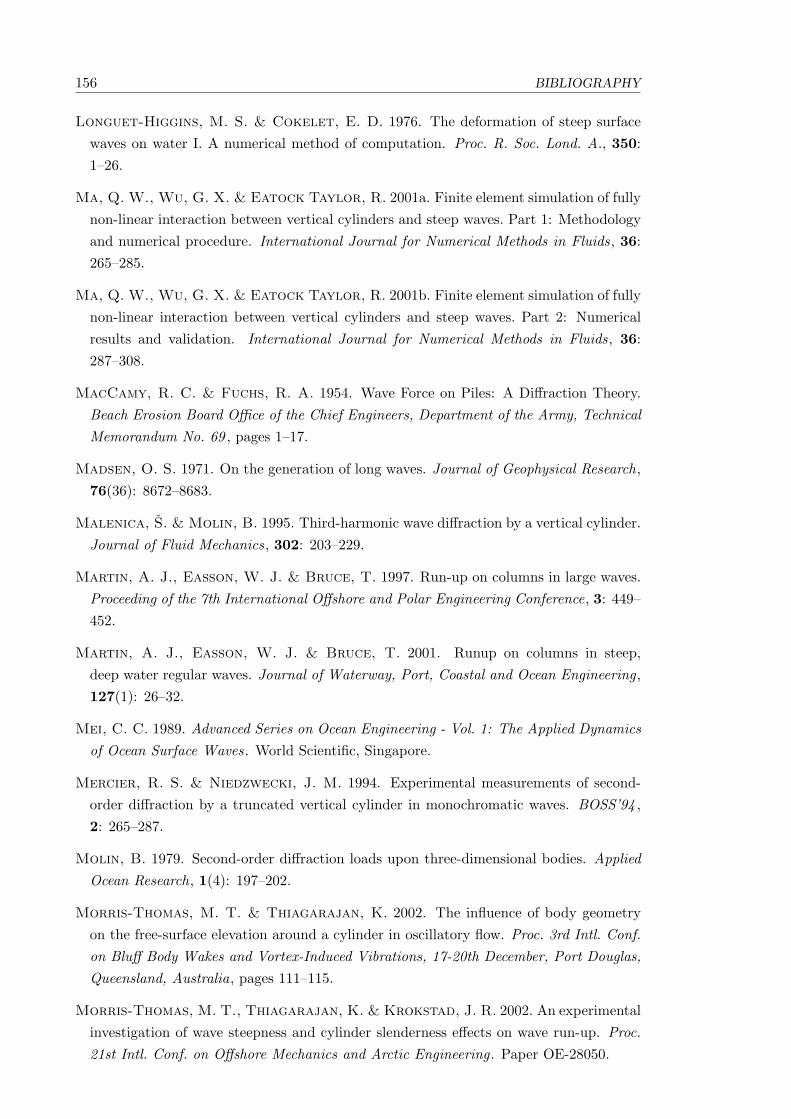
156 BIBLIOGRAPHY
Longuet-Higgins, M. S. & Cokelet, E. D. 1976. The deformation of steep surfacewaves on water I. A numerical method of computation. Proc. R. Soc. Lond. A., 350:1–26.
Ma, Q. W., Wu, G. X. & Eatock Taylor, R. 2001a. Finite element simulation of fullynon-linear interaction between vertical cylinders and steep waves. Part 1: Methodologyand numerical procedure. International Journal for Numerical Methods in Fluids, 36:265–285.
Ma, Q. W., Wu, G. X. & Eatock Taylor, R. 2001b. Finite element simulation of fullynon-linear interaction between vertical cylinders and steep waves. Part 2: Numericalresults and validation. International Journal for Numerical Methods in Fluids, 36:287–308.
MacCamy, R. C. & Fuchs, R. A. 1954. Wave Force on Piles: A Diffraction Theory.Beach Erosion Board Office of the Chief Engineers, Department of the Army, TechnicalMemorandum No. 69 , pages 1–17.
Madsen, O. S. 1971. On the generation of long waves. Journal of Geophysical Research,76(36): 8672–8683.
Malenica, S. & Molin, B. 1995. Third-harmonic wave diffraction by a vertical cylinder.Journal of Fluid Mechanics, 302: 203–229.
Martin, A. J., Easson, W. J. & Bruce, T. 1997. Run-up on columns in large waves.Proceeding of the 7th International Offshore and Polar Engineering Conference, 3: 449–452.
Martin, A. J., Easson, W. J. & Bruce, T. 2001. Runup on columns in steep,deep water regular waves. Journal of Waterway, Port, Coastal and Ocean Engineering,127(1): 26–32.
Mei, C. C. 1989. Advanced Series on Ocean Engineering - Vol. 1: The Applied Dynamicsof Ocean Surface Waves. World Scientific, Singapore.
Mercier, R. S. & Niedzwecki, J. M. 1994. Experimental measurements of second-order diffraction by a truncated vertical cylinder in monochromatic waves. BOSS’94 ,2: 265–287.
Molin, B. 1979. Second-order diffraction loads upon three-dimensional bodies. AppliedOcean Research, 1(4): 197–202.
Morris-Thomas, M. T. & Thiagarajan, K. 2002. The influence of body geometryon the free-surface elevation around a cylinder in oscillatory flow. Proc. 3rd Intl. Conf.on Bluff Body Wakes and Vortex-Induced Vibrations, 17-20th December, Port Douglas,Queensland, Australia, pages 111–115.
Morris-Thomas, M. T., Thiagarajan, K. & Krokstad, J. R. 2002. An experimentalinvestigation of wave steepness and cylinder slenderness effects on wave run-up. Proc.21st Intl. Conf. on Offshore Mechanics and Arctic Engineering. Paper OE-28050.

BIBLIOGRAPHY 157
Newland, D. E. 1993. An Introduction to Random Vibrations, Spectral and WaveletAnalysis. Longman Scientific & Technical, New York.
Newman, J. N. 1977. Marine Hydrodynamics. MIT Press, Cambridge, Massachusetts.
Newman, J. N. 1992. Panel methods in marine hydrodynamics. 11th Australasian FluidMechanics Conference, University of Tasmania, Hobart, Australia, 1: 123–130.
Newman, J. N. 1996a. Nonlinear scattering of long waves by a vertical cylinder. Wavesand Non-linear Processes in Hydrodynamics, pages 91–102. Edited by J. Grue et al.
Newman, J. N. 1996b. Second-order wave force on a vertical cylinder. Journal of FluidMechanics, 320: 417–443.
Newman, J. N. & Lee, C. H. 1992. Sensitivity of wave loads to the discretization ofbodies. Behaviour of Offshore Structures, BOSS ’92 , pages 50–64.
Newman, J. N. & Lee, C. H. 1995. Runup on a vertical cylinder in long waves. 10thWorkshop on Water Waves and Floating Bodies, Oxford, UK , pages 198–191.
Newman, J. N. & Lee, C. H. 2001. Boundary-element methods in offshore structureanalysis. 20th International Conference on Offshore Mechanics and Arctic Engineering,Rio de Janeiro, Brazil , pages 1–13.
Niedzwecki, J. M. & Duggal, A. S. 1990. Wave runup and wave forces on a truncatedcylinder. 22nd Annual Offshore Technology Conference, Houston, Texas, pages 615–634.
Niedzwecki, J. M. & Duggal, A. S. 1992. Wave runup and forces on cylinders inregular and random waves. Journal of Waterway, Port, Coastal, and Ocean Engineering,118(6): 615–634.
Niedzwecki, J. M. & Huston, J. R. 1992. Wave interaction with Tension Leg Plat-forms. Ocean Engineering , 19: 21–37.
Nielsen, F. G. 2000. Comparative study of airgap under floating platforms and run-upon platform columns. Unpublished, Norsk Hydro Research Centre.
Nielsen, F. G. 2003. Comparative Study on airgap under floating platforms and run-upalong platform columns. Marine Structures, 16: 97–134.
Ogilvie, T. F. 1983. Second-order hydrodynamics effects on ocean platforms. Proc.International Workshop on Ship and Platform Motions, 243: 205–265.
OPL. 1991. Diving Support Vessel of the World . Oil Field Publications Limited, Ledbury,England, 2 edition.
OPL. 1996. The World offshore Field Development Guide. Oil Field Publications Limited,Ledbury, England, 2nd edition.
Park, J.-H., Kim, M.-H. & Miyata, H. 1999. Fully Non-linear free-surface simulationby a 3-D viscous numerical wave tank. International Journal for Numerical Methods inFluids, 29: 685–703.

158 BIBLIOGRAPHY
Price, W. H., Teukolsky, S. A., Vetterling, W. T. & Flannery, B. P. 1992. Nu-merical Recipes in FORTRAN: The Art of Scientific Computing, volume 1. CambridgeUniversity Press, New York, 2 edition.
Prudnikov, A. P., Brychkov, Y. A. & Marichev, O. I. 1986. Integrals and SeriesVolume 2: Special Functions. Gordon and Breach Science Publishers, New York.
Prudnikov, A. P., Brychkov, Y. A. & Marichev, O. I. 1990. Integrals and SeriesVolume 3: More Special Functions. Gordon and Breach Science Publishers, New York.
Rainey, R. C. T. 1997. Violent surface motions around vertical cylinders in large, steepwaves - is this the result of the step change in relative acceleration? Proc. 12th Intl.Workshop on Water Waves and Floating Bodies, Marseilles, France, pages 215–218.
Retzler, C. H., Chaplin, J. R. & Rainey, R. C. T. 2000. Transient motion of avertical cylinder: Measurements and computations of the free-surface. Proceedings ofthe Fifteenth International Workshop on Water Waves and Floating Bodies, Universityof Michigan, April 11-14 , pages 154–157.
Sarpkaya, T. & Isaacson, M. de St Q. 1981. Mechanics of Wave Forces on OffshoreStructures. Van Nostrand Reinhold Company, New York.
Schaffer, H. A. 1996. Second-order wave maker theory for irregular waves. OceanEngineering , 23(1): 47–88.
Schwartz, L. W. 1974. Computer extension and analytic continuation of Stokes’s ex-pansion for gravity waves. Journal of Fluid Mechanics, 62: 553–578.
Seguin, B. 1999. Run-up av bølger pa sylindre med ulike tversnitt . Master’s thesis, Norgesteknisk-naturvitenskapelige universitet.
Shore Protection Manual. 1984. U.S. Government Printing Office, Washington D.C. 20402,4th edition. Department of the Army Waterways Experimental Station, Corps of Engi-neers.
Solaas, F. & Krokstad, J. R. 2000. Deep Water Analysis Tool - Enhanced Perturba-tion Based Ringing Model. Technical Report 513101.34.01, MARINTEK, Trondheim,Norway.
Stansberg, C. T. 2002. Personal Communication.
Stansberg, C. T. & Braaten, H. 2002. Nonlinear wave disturbance around a verticalcircular column. Proc. 21st Intl. Conf. Offshore Mechanics and Arctic Engineering,(paper 28620). June 23-28, Oslo, Norway.
Stansberg, C. T. & Nielsen, F. G. 2001. Nonlinear wave-structure interaction onfloating production systems. Proceedings of the 11th International Offshore and PolarEngineering Conference, Japan, 3: 363–372.

BIBLIOGRAPHY 159
Stoker, J. J. 1957. Water Waves: The Mathematical Theory with Applications. Inter-science Publishers, Inc., New York.
Sundar, V. & Mathai, T. 1985. Wave force and wave runup on elliptical cylinders.Proceedings of the International Symposium on Ocean Space Utilization ’85 , 1: 155–162.
Swan, C., Taylor, P. H. & van Langen, H. 1997. Observations of wave-structureinteraction for a multi-legged concrete platform. Applied Ocean Research, 19: 309–327.
Teigen, P. & Trulsen, K. 2001. Numerical investigation of wave effects around mul-tiple cylinders. Proceedings of the 11th International Offshore and Polar EngineeringConference, Stavanger, Norway, June 17-22 , 3: 369–378.
WAMIT. 1995. WAMIT v5.3: A Radiation-Diffraction Panel Program for Wave-BodyInteractions. Report, Massachusetts Institute of Technology.
Watson, G. N. 1962. A Treatise on the Theory of Bessel Functions. Cambridge Univer-sity Press, London, England, 2nd edition.
Wehausen, J. V. & Laitone, E. V. 1960. Surface Waves. Handbuch der Physik , 9:446–758.
Whitham, G. B. 1974. Linear and Nonlinear Waves. John Wiley & Sons, Inc., NewYork.
Williams, J. M. 1980. Limiting gravity waves in water of finite depth. Proc. R. Soc.Lond. A, 302: 139–188.
Xia, J. 2001. Evaluation of the Green function for 3-D wave-body interactions in achannel. To appear, The University of Western Australia.
Xue, M., Xu, H. B., Liu, Y. & Yue, D. K. P. 2001. Computations of fully nonlinearthree-dimensional wave-wave and wave-body interactions, Part 1: Three-dimensionalsteep waves. Journal of Fluid Mechanics, 438: 11–39.

Appendix A
Additional Experimental Results
A.1 Confidence Levels

A.1. CONFIDENCE LEVELS 161
Table A.1: Level of confidence for each wave probe pertaining to the circular cylinder. Thevalues given represent the maximum wave amplitude recorded divided by the mean of the waveamplitudes. RWP: Repeatability wave probe; PWP: Phase wave probe. The wave probe positionsare given in Table 2.3.
ka kA RWP PWP A1 A2 A3 A4 B1 C11.386 0.206 1.096 1.172 1.240 1.152 1.136 1.422 1.242 1.0560.698 0.284 1.026 1.026 1.035 1.048 1.029 1.027 1.019 1.0160.417 0.263 1.039 1.015 1.064 1.021 1.040 1.054 1.069 1.0320.283 0.228 1.017 1.019 1.046 1.024 1.026 1.025 1.037 1.0250.208 0.233 1.011 1.005 1.045 1.028 1.047 1.043 1.014 1.0331.386 0.206 1.104 1.197 1.219 1.096 1.089 1.246 1.256 1.1080.698 0.261 1.064 1.036 1.040 1.110 1.057 1.034 1.031 1.0420.417 0.244 1.068 1.045 1.043 1.014 1.120 1.106 1.051 1.0660.283 0.225 1.048 1.034 1.108 1.051 1.040 1.037 1.063 1.0670.208 0.231 1.031 1.000 1.045 1.021 1.028 1.042 1.090 1.0321.386 0.143 1.053 1.080 1.100 1.110 1.141 1.342 1.111 1.0290.698 0.233 1.032 1.050 1.053 1.080 1.110 1.070 1.034 1.0130.417 0.213 1.023 1.018 1.050 1.032 1.073 1.159 1.039 1.0690.283 0.180 1.091 1.034 1.059 1.041 1.020 1.011 1.075 1.0520.208 0.200 1.045 1.033 1.077 1.073 1.054 1.046 1.078 1.0311.386 0.157 1.034 1.073 1.154 1.123 1.125 1.156 1.038 1.0700.698 0.212 1.044 1.034 1.063 1.028 1.065 1.056 1.025 1.0370.417 0.200 1.039 1.015 1.049 1.052 1.038 1.123 1.030 1.0280.283 0.172 1.111 1.037 1.036 1.024 1.042 1.036 1.028 1.0390.208 0.185 1.023 1.033 1.035 1.056 1.037 1.034 1.027 1.0221.386 0.109 1.077 1.210 1.245 1.090 1.385 1.951 1.105 1.2190.698 0.179 1.091 1.050 1.059 1.051 1.074 1.137 1.040 1.0570.417 0.166 1.037 1.023 1.065 1.044 1.021 1.089 1.057 1.0890.283 0.140 1.068 1.034 1.039 1.035 1.027 1.023 1.081 1.0330.208 0.160 1.030 1.056 1.090 1.074 1.063 1.075 1.057 1.0641.386 0.104 1.096 1.077 1.088 1.060 1.086 1.295 1.059 1.0520.698 0.162 1.057 1.025 1.054 1.040 1.040 1.045 1.023 1.0100.417 0.156 1.034 1.028 1.032 1.024 1.028 1.027 1.024 1.0240.283 0.133 1.044 1.013 1.044 1.041 1.025 1.023 1.053 1.0360.208 0.152 1.029 1.023 1.031 1.032 1.048 1.042 1.030 1.0931.386 0.041 1.069 1.048 1.065 1.068 1.077 1.173 1.035 1.0850.698 0.062 1.027 1.034 1.024 1.024 1.080 1.057 1.042 1.0280.417 0.057 1.027 1.012 1.026 1.017 1.025 1.022 1.033 1.0370.283 0.047 1.019 1.023 1.013 1.027 1.020 1.011 1.033 1.0210.208 0.055 1.015 1.019 1.043 1.049 1.041 1.054 1.029 1.020

162 APPENDIX A. ADDITIONAL EXPERIMENTAL RESULTS
Table A.2: Cylinder B, rc/a = 0.75: Level of confidence for each wave probe. The values givenrepresent the maximum wave amplitude recorded divided by the mean of the wave amplitudes.RWP: Repeatability wave probe; PWP: Phase wave probe.
ka kA RWP PWP A1 A2 A3 A4 B1 C11.386 0.250 1.125 1.092 1.331 1.105 1.263 1.136 1.298 1.0980.698 0.284 1.052 1.049 1.116 1.099 1.066 1.018 1.050 1.0370.417 0.273 1.049 1.017 1.036 1.009 1.040 1.017 1.048 1.0560.283 0.232 1.042 1.063 1.063 1.029 1.023 1.039 1.038 1.0540.208 0.228 1.016 1.001 1.019 1.035 1.035 1.051 1.074 1.0431.386 0.202 1.086 1.116 1.126 1.095 1.114 1.164 1.303 1.0920.698 0.249 1.028 1.035 1.057 1.026 1.039 1.040 1.027 1.0170.417 0.225 1.058 1.020 1.040 1.026 1.033 1.031 1.071 1.0430.283 0.199 1.070 1.029 1.069 1.037 1.025 1.022 1.066 1.0660.208 0.222 1.066 1.034 1.109 1.078 1.048 1.055 1.114 1.0671.386 0.127 1.115 1.074 1.160 1.154 1.189 1.280 1.066 1.2370.698 0.194 1.076 1.021 1.046 1.080 1.123 1.101 1.035 1.0800.417 0.184 1.061 1.010 1.027 1.036 1.037 1.049 1.035 1.0580.283 0.151 1.043 1.024 1.021 1.023 1.023 1.028 1.028 1.0600.208 0.176 1.079 1.088 1.116 1.081 1.067 1.048 1.070 1.0301.477 0.100 1.061 1.036 1.115 1.147 1.138 1.379 1.022 1.0150.698 0.152 1.076 1.038 1.045 1.040 1.058 1.055 1.036 1.0220.417 0.145 1.019 1.023 1.032 1.031 1.019 1.017 1.015 1.0570.283 0.120 1.093 1.021 1.044 1.045 1.029 1.025 1.059 1.0510.208 0.140 1.055 1.121 1.035 1.025 1.041 1.029 1.027 1.055
Table A.3: Cylinder C, rc/a = 0.5: Level of confidence for each wave probe. The values givenrepresent the maximum wave amplitude recorded divided by the mean of the wave amplitudes.RWP: Repeatability wave probe; PWP: Phase wave probe.
ka kA RWP PWP A1 A2 A3 A4 B1 C11.386 0.252 1.201 1.214 1.234 1.255 1.205 1.187 1.120 1.0590.698 0.291 1.030 1.043 1.083 1.058 1.076 1.049 1.043 1.0430.417 0.271 1.031 1.018 1.031 1.041 1.035 1.018 1.039 1.0330.283 0.235 1.040 1.093 1.103 1.035 1.039 1.025 1.076 1.0330.208 0.226 1.012 1.000 1.008 1.053 1.065 1.046 1.078 1.0411.386 0.197 1.039 1.087 1.143 1.130 1.221 1.272 1.088 1.0680.698 0.250 1.029 1.036 1.036 1.066 1.059 1.061 1.036 1.0240.417 0.231 1.047 1.017 1.052 1.028 1.032 1.030 1.060 1.0280.283 0.196 1.053 1.035 1.063 1.037 1.037 1.033 1.062 1.0530.208 0.223 1.093 1.058 1.190 1.131 1.063 1.047 1.165 1.1201.386 0.120 1.036 1.037 1.061 1.056 1.189 1.346 1.045 1.0740.698 0.199 1.056 1.025 1.031 1.040 1.027 1.030 1.023 1.0230.417 0.186 1.037 1.012 1.031 1.040 1.023 1.036 1.031 1.0270.283 0.151 1.061 1.034 1.041 1.031 1.029 1.034 1.036 1.0420.208 0.174 1.044 1.048 1.068 1.075 1.049 1.049 1.065 1.0341.477 0.092 1.062 1.020 1.105 1.077 1.067 1.097 1.051 1.0640.698 0.154 1.041 1.019 1.030 1.019 1.032 1.017 1.032 1.0190.417 0.146 1.032 1.013 1.020 1.024 1.019 1.010 1.020 1.0430.283 0.118 1.096 1.257 1.031 1.033 1.032 1.031 1.040 1.0420.208 0.138 1.028 1.121 1.014 1.030 1.033 1.037 1.037 1.040

A.1. CONFIDENCE LEVELS 163
Table A.4: Cylinder D, rc/a = 0.25: Level of confidence for each wave probe. The values givenrepresent the maximum wave amplitude recorded divided by the mean of the wave amplitudes.RWP: Repeatability wave probe; PWP: Phase wave probe.
ka kA RWP PWP A1 A2 A3 A4 B1 C11.386 0.196 1.104 1.194 1.210 1.130 1.156 1.408 1.181 1.1550.698 0.284 1.051 1.078 1.117 1.142 1.070 1.071 1.050 1.0530.417 0.288 1.035 1.035 1.093 1.061 1.025 1.041 1.085 1.0330.283 0.230 1.058 1.029 1.106 1.039 1.053 1.057 1.048 1.0730.208 0.228 1.023 1.002 1.041 1.045 1.035 1.040 1.081 1.0431.386 0.159 1.125 1.185 1.134 1.137 1.203 1.334 1.153 1.1740.698 0.254 1.029 1.021 1.041 1.039 1.033 1.030 1.026 1.0180.417 0.237 1.043 1.021 1.036 1.025 1.056 1.050 1.093 1.0380.283 0.194 1.074 1.062 1.047 1.028 1.053 1.041 1.064 1.0870.208 0.216 1.045 1.026 1.147 1.081 1.055 1.035 1.117 1.0621.386 0.117 1.111 1.068 1.057 1.030 1.030 1.085 1.057 1.0550.698 0.117 1.036 1.032 1.024 1.027 1.025 1.039 1.036 1.0160.417 0.191 1.035 1.028 1.028 1.026 1.033 1.019 1.022 1.0540.283 0.146 1.119 1.034 1.041 1.030 1.035 1.054 1.045 1.0340.208 0.175 1.052 1.048 1.085 1.072 1.054 1.032 1.043 1.0551.386 0.090 1.081 1.044 1.163 1.136 1.140 1.111 1.060 1.0990.698 0.150 1.093 1.074 1.021 1.021 1.047 1.067 1.045 1.0260.417 0.147 1.020 1.018 1.013 1.010 1.011 1.017 1.017 1.0500.283 0.116 1.292 1.032 1.021 1.018 1.037 1.036 1.035 1.0220.208 0.136 1.033 1.123 1.031 1.027 1.010 1.017 1.040 1.040
Table A.5: Cylinder E, rc/a = 0: Level of confidence for each wave probe. The values givenrepresent the maximum wave amplitude recorded divided by the mean of the wave amplitudes.RWP: Repeatability wave probe; PWP: Phase wave probe.
ka kA RWP PWP A1 A2 A3 A4 B1 C11.386 0.263 1.056 1.169 1.207 1.187 1.202 1.464 1.165 1.0970.698 0.272 1.045 1.031 1.025 1.082 1.137 1.165 1.059 1.0720.417 0.273 1.024 1.024 1.052 1.028 1.024 1.031 1.037 1.0440.283 0.239 1.040 1.062 1.092 1.075 1.022 1.032 1.052 1.0600.208 0.227 1.023 1.004 1.026 1.043 1.039 1.034 1.025 1.0511.386 0.213 1.050 1.081 1.092 1.056 1.109 1.208 1.064 1.1340.698 0.245 1.012 1.085 1.046 1.022 1.029 1.044 1.028 1.0490.417 0.235 1.018 1.057 1.009 1.019 1.020 1.020 1.036 1.0290.283 0.200 1.089 1.060 1.049 1.038 1.028 1.027 1.043 1.0510.208 0.217 1.119 1.074 1.078 1.074 1.062 1.058 1.048 1.0601.386 0.112 1.037 1.025 1.078 1.035 1.085 1.154 1.026 1.0800.698 0.188 1.075 1.030 1.037 1.036 1.029 1.045 1.020 1.0410.417 0.186 1.043 1.022 1.018 1.018 1.012 1.020 1.026 1.0290.283 0.149 1.087 1.024 1.064 1.060 1.047 1.016 1.034 1.0570.208 0.175 1.052 1.028 1.123 1.094 1.070 1.047 1.059 1.0461.477 0.094 1.105 1.026 1.127 1.128 1.134 1.100 1.039 1.0850.698 0.150 1.062 1.028 1.018 1.020 1.033 1.033 1.027 1.0150.417 0.149 1.014 1.016 1.019 1.015 1.009 1.012 1.041 1.0150.283 0.118 1.084 1.017 1.020 1.017 1.028 1.037 1.038 1.0340.208 0.139 1.028 1.048 1.033 1.035 1.043 1.021 1.058 1.047

164 APPENDIX A. ADDITIONAL EXPERIMENTAL RESULTS
A.2 Harmonic Components of the Wave Run-up
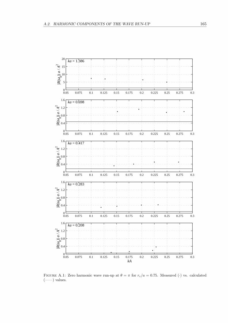
A.2. HARMONIC COMPONENTS OF THE WAVE RUN-UP 165
0.05 0.075 0.1 0.125 0.15 0.175 0.2 0.225 0.25 0.275 0.30
5
10
15
20|R
(ω0)|
a / A
2
ka = 1.386
0.05 0.075 0.1 0.125 0.15 0.175 0.2 0.225 0.25 0.275 0.30
0.4
0.8
1.2
1.6
|R(ω
0)| a
/ A2
ka = 0.698
0.05 0.075 0.1 0.125 0.15 0.175 0.2 0.225 0.25 0.275 0.30
0.4
0.8
1.2
1.6
|R(ω
0)| a
/ A2
ka = 0.417
0.05 0.075 0.1 0.125 0.15 0.175 0.2 0.225 0.25 0.275 0.30
0.4
0.8
1.2
1.6
|R(ω
0)| a
/ A2
ka = 0.283
0.05 0.075 0.1 0.125 0.15 0.175 0.2 0.225 0.25 0.275 0.30
0.4
0.8
1.2
1.6
kA
|R(ω
0)| a
/ A2
ka = 0.208
Figure A.1: Zero harmonic wave run-up at θ = π for rc/a = 0.75. Measured (·) vs. calculated(——) values.

166 APPENDIX A. ADDITIONAL EXPERIMENTAL RESULTS
0.05 0.075 0.1 0.125 0.15 0.175 0.2 0.225 0.25 0.275 0.30
5
10
15
20
|R(ω
0)| a
/ A2
ka = 1.386
0.05 0.075 0.1 0.125 0.15 0.175 0.2 0.225 0.25 0.275 0.30
0.4
0.8
1.2
1.6
|R(ω
0)| a
/ A2
ka = 0.698
0.05 0.075 0.1 0.125 0.15 0.175 0.2 0.225 0.25 0.275 0.30
0.4
0.8
1.2
1.6
|R(ω
0)| a
/ A2
ka = 0.417
0.05 0.075 0.1 0.125 0.15 0.175 0.2 0.225 0.25 0.275 0.30
0.4
0.8
1.2
1.6
|R(ω
0)| a
/ A2
ka = 0.283
0.05 0.075 0.1 0.125 0.15 0.175 0.2 0.225 0.25 0.275 0.30
0.4
0.8
1.2
1.6
kA
|R(ω
0)| a
/ A2
ka = 0.208
Figure A.2: Zero harmonic wave run-up at θ = π for rc/a = 0.5. Measured (·) vs. calculated(——) values.

A.2. HARMONIC COMPONENTS OF THE WAVE RUN-UP 167
0.05 0.075 0.1 0.125 0.15 0.175 0.2 0.225 0.25 0.275 0.30
5
10
15
20|R
(ω0)|
a / A
2
ka = 1.386
0.05 0.075 0.1 0.125 0.15 0.175 0.2 0.225 0.25 0.275 0.30
0.4
0.8
1.2
1.6
|R(ω
0)| a
/ A2
ka = 0.698
0.05 0.075 0.1 0.125 0.15 0.175 0.2 0.225 0.25 0.275 0.30
0.4
0.8
1.2
1.6
|R(ω
0)| a
/ A2
ka = 0.417
0.05 0.075 0.1 0.125 0.15 0.175 0.2 0.225 0.25 0.275 0.30
0.4
0.8
1.2
1.6
|R(ω
0)| a
/ A2
ka = 0.283
0.05 0.075 0.1 0.125 0.15 0.175 0.2 0.225 0.25 0.275 0.30
0.4
0.8
1.2
1.6
kA
|R(ω
0)| a
/ A2
ka = 0.208
Figure A.3: Zero harmonic wave run-up at θ = π for rc/a = 0.25. Measured (·) vs. calculated(——) values.

168 APPENDIX A. ADDITIONAL EXPERIMENTAL RESULTS
0.05 0.075 0.1 0.125 0.15 0.175 0.2 0.225 0.25 0.275 0.30
5
10
15
20
|R(ω
0)| a
/ A2
ka = 1.386
0.05 0.075 0.1 0.125 0.15 0.175 0.2 0.225 0.25 0.275 0.30
0.4
0.8
1.2
1.6
|R(ω
0)| a
/ A2
ka = 0.698
0.05 0.075 0.1 0.125 0.15 0.175 0.2 0.225 0.25 0.275 0.30
0.4
0.8
1.2
1.6
|R(ω
0)| a
/ A2
ka = 0.417
0.05 0.075 0.1 0.125 0.15 0.175 0.2 0.225 0.25 0.275 0.30
0.4
0.8
1.2
1.6
|R(ω
0)| a
/ A2
ka = 0.283
0.05 0.075 0.1 0.125 0.15 0.175 0.2 0.225 0.25 0.275 0.30
0.4
0.8
1.2
1.6
kA
|R(ω
0)| a
/ A2
ka = 0.208
Figure A.4: Zero-harmonic wave run-up at θ = π for rc/a = 0. Measured (·) vs. calculated(——) values.

A.2. HARMONIC COMPONENTS OF THE WAVE RUN-UP 169
0.05 0.075 0.1 0.125 0.15 0.175 0.2 0.225 0.25 0.275 0.31
1.75
2.5
3.25
4|R
(ω1)|
/ A ka = 1.386
0.05 0.075 0.1 0.125 0.15 0.175 0.2 0.225 0.25 0.275 0.30.4
0.8
1.2
1.6
2
|R(ω
1)| / A
ka = 0.698
0.05 0.075 0.1 0.125 0.15 0.175 0.2 0.225 0.25 0.275 0.30.4
0.8
1.2
1.6
2
|R(ω
1)| / A
ka = 0.417
0.05 0.075 0.1 0.125 0.15 0.175 0.2 0.225 0.25 0.275 0.30.4
0.8
1.2
1.6
2
|R(ω
1)| / A
ka = 0.283
0.05 0.075 0.1 0.125 0.15 0.175 0.2 0.225 0.25 0.275 0.30.4
0.8
1.2
1.6
2
kA
|R(ω
1)| / A
ka = 0.208
Figure A.5: First-harmonic modulus of the wave run-up at θ = π for rc/a = 0.75. Measured (·)vs. calculated (——) values.

170 APPENDIX A. ADDITIONAL EXPERIMENTAL RESULTS
0.05 0.075 0.1 0.125 0.15 0.175 0.2 0.225 0.25 0.275 0.31
1.75
2.5
3.25
4
|R(ω
1)| / A
ka = 1.386
0.05 0.075 0.1 0.125 0.15 0.175 0.2 0.225 0.25 0.275 0.30.4
0.8
1.2
1.6
2
|R(ω
1)| / A
ka = 0.698
0.05 0.075 0.1 0.125 0.15 0.175 0.2 0.225 0.25 0.275 0.30.4
0.8
1.2
1.6
2
|R(ω
1)| / A
ka = 0.417
0.05 0.075 0.1 0.125 0.15 0.175 0.2 0.225 0.25 0.275 0.30.4
0.8
1.2
1.6
2
|R(ω
1)| / A
ka = 0.283
0.05 0.075 0.1 0.125 0.15 0.175 0.2 0.225 0.25 0.275 0.30.4
0.8
1.2
1.6
2
kA
|R(ω
1)| / A
ka = 0.208
Figure A.6: First-harmonic modulus of the wave run-up at θ = π for rc/a = 0.5. Measured (·)vs. calculated (——) values.

A.2. HARMONIC COMPONENTS OF THE WAVE RUN-UP 171
0.05 0.075 0.1 0.125 0.15 0.175 0.2 0.225 0.25 0.275 0.31
1.75
2.5
3.25
4|R
(ω1)|
/ A ka = 1.386
0.05 0.075 0.1 0.125 0.15 0.175 0.2 0.225 0.25 0.275 0.30.4
0.8
1.2
1.6
2
|R(ω
1)| / A
ka = 0.698
0.05 0.075 0.1 0.125 0.15 0.175 0.2 0.225 0.25 0.275 0.30.4
0.8
1.2
1.6
2
|R(ω
1)| / A
ka = 0.417
0.05 0.075 0.1 0.125 0.15 0.175 0.2 0.225 0.25 0.275 0.30.4
0.8
1.2
1.6
2
|R(ω
1)| / A
ka = 0.283
0.05 0.075 0.1 0.125 0.15 0.175 0.2 0.225 0.25 0.275 0.30.4
0.8
1.2
1.6
2
kA
|R(ω
1)| / A
ka = 0.208
Figure A.7: First-harmonic modulus of the wave run-up at θ = π for rc/a = 0.25. Measured (·)vs. calculated (——) values.

172 APPENDIX A. ADDITIONAL EXPERIMENTAL RESULTS
0.05 0.075 0.1 0.125 0.15 0.175 0.2 0.225 0.25 0.275 0.31
1.75
2.5
3.25
4
|R(ω
1)| / A
ka = 1.386
0.05 0.075 0.1 0.125 0.15 0.175 0.2 0.225 0.25 0.275 0.30.4
0.8
1.2
1.6
2
|R(ω
1)| / A
ka = 0.698
0.05 0.075 0.1 0.125 0.15 0.175 0.2 0.225 0.25 0.275 0.30.4
0.8
1.2
1.6
2
|R(ω
1)| / A
ka = 0.417
0.05 0.075 0.1 0.125 0.15 0.175 0.2 0.225 0.25 0.275 0.30.4
0.8
1.2
1.6
2
|R(ω
1)| / A
ka = 0.283
0.05 0.075 0.1 0.125 0.15 0.175 0.2 0.225 0.25 0.275 0.30.4
0.8
1.2
1.6
2
kA
|R(ω
1)| / A
ka = 0.208
Figure A.8: First-harmonic modulus of the wave run-up at θ = π for rc/a = 0. Measured (·) vs.calculated (——) values.

A.2. HARMONIC COMPONENTS OF THE WAVE RUN-UP 173
0.05 0.075 0.1 0.125 0.15 0.175 0.2 0.225 0.25 0.275 0.30
0.8
1.6
2.4
3.2|R
(ω2)|
a / A
2
ka = 1.386
0.05 0.075 0.1 0.125 0.15 0.175 0.2 0.225 0.25 0.275 0.30
0.3
0.6
0.9
1.2
|R(ω
2)| a
/ A2
ka = 0.698
0.05 0.075 0.1 0.125 0.15 0.175 0.2 0.225 0.25 0.275 0.30
0.3
0.6
0.9
1.2
|R(ω
2)| a
/ A2
ka = 0.417
0.05 0.075 0.1 0.125 0.15 0.175 0.2 0.225 0.25 0.275 0.30
0.3
0.6
0.9
1.2
|R(ω
2)| a
/ A2
ka = 0.283
0.05 0.075 0.1 0.125 0.15 0.175 0.2 0.225 0.25 0.275 0.30
0.3
0.6
0.9
1.2
kA
|R(ω
2)| a
/ A2
ka = 0.208
Figure A.9: Second-harmonic modulus of the wave run-up at θ = π for rc/a = 0.75. Measured(·) vs. calculated (——) values.
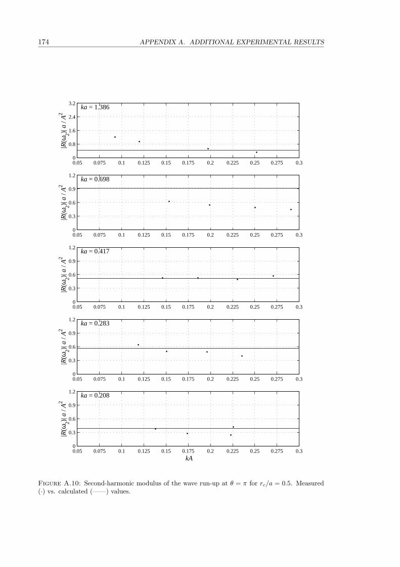
174 APPENDIX A. ADDITIONAL EXPERIMENTAL RESULTS
0.05 0.075 0.1 0.125 0.15 0.175 0.2 0.225 0.25 0.275 0.30
0.8
1.6
2.4
3.2
|R(ω
2)| a
/ A2
ka = 1.386
0.05 0.075 0.1 0.125 0.15 0.175 0.2 0.225 0.25 0.275 0.30
0.3
0.6
0.9
1.2
|R(ω
2)| a
/ A2
ka = 0.698
0.05 0.075 0.1 0.125 0.15 0.175 0.2 0.225 0.25 0.275 0.30
0.3
0.6
0.9
1.2
|R(ω
2)| a
/ A2
ka = 0.417
0.05 0.075 0.1 0.125 0.15 0.175 0.2 0.225 0.25 0.275 0.30
0.3
0.6
0.9
1.2
|R(ω
2)| a
/ A2
ka = 0.283
0.05 0.075 0.1 0.125 0.15 0.175 0.2 0.225 0.25 0.275 0.30
0.3
0.6
0.9
1.2
kA
|R(ω
2)| a
/ A2
ka = 0.208
Figure A.10: Second-harmonic modulus of the wave run-up at θ = π for rc/a = 0.5. Measured(·) vs. calculated (——) values.

A.2. HARMONIC COMPONENTS OF THE WAVE RUN-UP 175
0.05 0.075 0.1 0.125 0.15 0.175 0.2 0.225 0.25 0.275 0.30
0.8
1.6
2.4
3.2|R
(ω2)|
a / A
2
ka = 1.386
0.05 0.075 0.1 0.125 0.15 0.175 0.2 0.225 0.25 0.275 0.30
0.3
0.6
0.9
1.2
|R(ω
2)| a
/ A2
ka = 0.698
0.05 0.075 0.1 0.125 0.15 0.175 0.2 0.225 0.25 0.275 0.30
0.3
0.6
0.9
1.2
|R(ω
2)| a
/ A2
ka = 0.417
0.05 0.075 0.1 0.125 0.15 0.175 0.2 0.225 0.25 0.275 0.30
0.3
0.6
0.9
1.2
|R(ω
2)| a
/ A2
ka = 0.283
0.05 0.075 0.1 0.125 0.15 0.175 0.2 0.225 0.25 0.275 0.30
0.3
0.6
0.9
1.2
kA
|R(ω
2)| a
/ A2
ka = 0.208
Figure A.11: Second-harmonic modulus of the wave run-up at θ = π for rc/a = 0.25. Measured(·) vs. calculated (——) values.

176 APPENDIX A. ADDITIONAL EXPERIMENTAL RESULTS
0.05 0.075 0.1 0.125 0.15 0.175 0.2 0.225 0.25 0.275 0.30
0.8
1.6
2.4
3.2
|R(ω
2)| a
/ A2
ka = 1.386
0.05 0.075 0.1 0.125 0.15 0.175 0.2 0.225 0.25 0.275 0.30
0.3
0.6
0.9
1.2
|R(ω
2)| a
/ A2
ka = 0.698
0.05 0.075 0.1 0.125 0.15 0.175 0.2 0.225 0.25 0.275 0.30
0.3
0.6
0.9
1.2
|R(ω
2)| a
/ A2
ka = 0.417
0.05 0.075 0.1 0.125 0.15 0.175 0.2 0.225 0.25 0.275 0.30
0.3
0.6
0.9
1.2
|R(ω
2)| a
/ A2
ka = 0.283
0.05 0.075 0.1 0.125 0.15 0.175 0.2 0.225 0.25 0.275 0.30
0.3
0.6
0.9
1.2
kA
|R(ω
2)| a
/ A2
ka = 0.208
Figure A.12: Second-harmonic modulus of the wave run-up at θ = π for rc/a = 0. Measured (·)vs. calculated (——) values.

A.2. HARMONIC COMPONENTS OF THE WAVE RUN-UP 177
0.05 0.075 0.1 0.125 0.15 0.175 0.2 0.225 0.25 0.275 0.30
0.25
0.5
0.75
1|R
(ω3)|
a2 / A
3
ka = 0.698
0.05 0.075 0.1 0.125 0.15 0.175 0.2 0.225 0.25 0.275 0.30
0.25
0.5
0.75
1
|R(ω
3)| a2 /
A3
ka = 0.417
0.05 0.075 0.1 0.125 0.15 0.175 0.2 0.225 0.25 0.275 0.30
0.25
0.5
0.75
1
|R(ω
3)| a2 /
A3
ka = 0.283
0.05 0.075 0.1 0.125 0.15 0.175 0.2 0.225 0.25 0.275 0.30
0.25
0.5
0.75
1
kA
|R(ω
3)| a2 /
A3
ka = 0.208
Figure A.13: Third-harmonic modulus of the wave run-up at θ = π for rc/a = 0.75. Measuredvalues, (·).

178 APPENDIX A. ADDITIONAL EXPERIMENTAL RESULTS
0.05 0.075 0.1 0.125 0.15 0.175 0.2 0.225 0.25 0.275 0.30
0.25
0.5
0.75
1
|R(ω
3)| a2 /
A3
ka = 0.698
0.05 0.075 0.1 0.125 0.15 0.175 0.2 0.225 0.25 0.275 0.30
0.25
0.5
0.75
1
|R(ω
3)| a2 /
A3
ka = 0.417
0.05 0.075 0.1 0.125 0.15 0.175 0.2 0.225 0.25 0.275 0.30
0.25
0.5
0.75
1
|R(ω
3)| a2 /
A3
ka = 0.283
0.05 0.075 0.1 0.125 0.15 0.175 0.2 0.225 0.25 0.275 0.30
0.25
0.5
0.75
1
kA
|R(ω
3)| a2 /
A3
ka = 0.208
Figure A.14: Third-harmonic modulus of the wave run-up at θ = π for rc/a = 0.5. Measuredvalues, (·).

A.2. HARMONIC COMPONENTS OF THE WAVE RUN-UP 179
0.05 0.075 0.1 0.125 0.15 0.175 0.2 0.225 0.25 0.275 0.30
0.25
0.5
0.75
1|R
(ω3)|
a2 / A
3
ka = 0.698
0.05 0.075 0.1 0.125 0.15 0.175 0.2 0.225 0.25 0.275 0.30
0.25
0.5
0.75
1
|R(ω
3)| a2 /
A3
ka = 0.417
0.05 0.075 0.1 0.125 0.15 0.175 0.2 0.225 0.25 0.275 0.30
0.25
0.5
0.75
1
|R(ω
3)| a2 /
A3
ka = 0.283
0.05 0.075 0.1 0.125 0.15 0.175 0.2 0.225 0.25 0.275 0.30
0.25
0.5
0.75
1
kA
|R(ω
3)| a2 /
A3
ka = 0.208
Figure A.15: Third-harmonic modulus of the wave run-up at θ = π for rc/a = 0.25. Measuredvalues, (·)
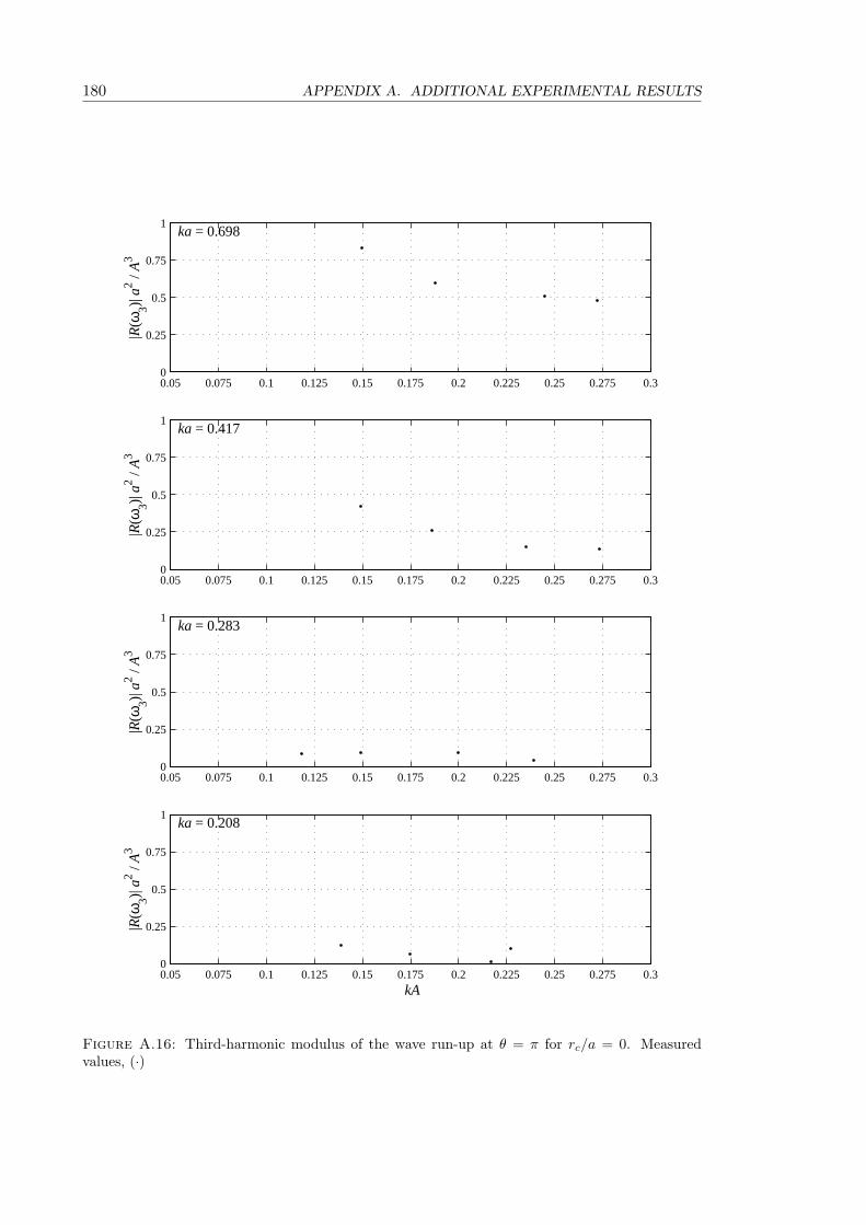
180 APPENDIX A. ADDITIONAL EXPERIMENTAL RESULTS
0.05 0.075 0.1 0.125 0.15 0.175 0.2 0.225 0.25 0.275 0.30
0.25
0.5
0.75
1
|R(ω
3)| a2 /
A3
ka = 0.698
0.05 0.075 0.1 0.125 0.15 0.175 0.2 0.225 0.25 0.275 0.30
0.25
0.5
0.75
1
|R(ω
3)| a2 /
A3
ka = 0.417
0.05 0.075 0.1 0.125 0.15 0.175 0.2 0.225 0.25 0.275 0.30
0.25
0.5
0.75
1
|R(ω
3)| a2 /
A3
ka = 0.283
0.05 0.075 0.1 0.125 0.15 0.175 0.2 0.225 0.25 0.275 0.30
0.25
0.5
0.75
1
kA
|R(ω
3)| a2 /
A3
ka = 0.208
Figure A.16: Third-harmonic modulus of the wave run-up at θ = π for rc/a = 0. Measuredvalues, (·)