
AN INVESTIGATION INTO THE FRICTION STIR...
193
AN INVESTIGATION INTO THE FRICTION STIR WELDING OF AL 6061 AND AL 6061/SiC/17.5p USING DIAMOND COATINGS By Tracie Prater Thesis Submitted to the Faculty of the Graduate School of Vanderbilt University in partial fulfillment of the requirements for the degree of MASTER OF SCIENCE in Mechanical Engineering August, 2008 Nashville, Tennessee Approved: Professor Alvin M. Strauss Professor George E. Cook
Transcript of AN INVESTIGATION INTO THE FRICTION STIR...
AN INVESTIGATION INTO THE FRICTION STIR WELDING OF AL 6061 AND
AL 6061/SiC/17.5p USING DIAMOND COATINGS
By
Tracie Prater
Thesis
Submitted to the Faculty of the
Graduate School of Vanderbilt University
in partial fulfillment of the requirements
for the degree of
MASTER OF SCIENCE
in
Mechanical Engineering
August, 2008
Nashville, Tennessee
Approved:
Professor Alvin M. Strauss
Professor George E. Cook

To my mother, grandmother, and Mrs. Beulah Hall
ii
ACKNOWLEDGEMENTS
I would like to take this opportunity to briefly recognize the myriad of people and
agencies which have helped me with this research during the paSt two years. My
research advisors, Drs. Al Straus and George E. Cook; Dr. Jim Davidson and Mick
Howell of the Diamond Fabrication Laboratory at Vanderbilt University; my labmates
Paul Fleming, David Lammlein, Thomas Bloodworth, and Paul Sinclair; Andrew
Bouchard for assistance with CAD; the Vanderbilt University machine shop; Estevan
Bunker for the photos and much of the information on experimental procedure; Midwest
Tungsten of Chicago, Illinois; sp3 for diamond coatings; DWA Composites of
Chatsworth, California for donated material; NASA Space Grant, which provided
financial support throughout this project; the NASA Academy program; Drs. Frank Six,
Alan Chow, and Art Nunes at Marshall Space Flight Center in Huntsville, Alabama for
the opportunities they have given me; Drs. Jerry Cook and Garrett Yoder, my
undergraduate physics professors; my family, friends, and pets for their patience and
support.
iii
TABLE OF CONTENTS
Page
DEDICATION…………………………………………………………………………….ii
ACKNOWLEDGEMENTS…………….………………………………………………...iii
LIST OF TABLES……………………………………………………………………......vi
LIST OF FIGURES……………………………………………………………………..viii
LIST OF ABBREVIATIONS…………………………………………………………..xiii
Chapter
I. INTRODUCTION…………………….………………………………........................1
Overview of the FSW Process…………..………………………………………….1 FSW Tools………………………………..………………………………………...2 FSW Workpieces with Emphasis on Metal Matrix Composites (MMCs)………....4 Diamond Coating by CVD (Chemical Vapor Deposition)……………………..…..6 Microstructural Zones………………………………………..……………………11 II. LITERATURE REVIEW……………………………………………………………13
III. EXPERIMENTAL PROCEDURE………………………………………………….45
Overview of the FSW Apparatus………………………………………………....45 Lateral, Traverse, Vertical Motors and Position Control………………………....49 Post-weld Analysis: Metallography………………………………………………54 Post-weld Analysis: Tensile Testing……………………………………………...55 Shadowgraph……………………………………………………………………...57 IV. EXPERIMENTAL RESULTS FOR SMOOTH PROBE FSW TOOLS ON AL 6061...…………………………………………………………………………..58 Tool Design………………………………………………………………………58 Parameter Selection……………………………………………………………...60 Results: General Trends in Force Data for the Uncoated Steel Smooth Probe FSW Tool………………………………………………………………………...64 Results: Force Data for Diamond Coated Smooth Probe FSW Tool…...……….68 Results: Comparison of Data for Coated and Uncoated Smooth Probe FSW Tools………………………………………………...…………………………...74
iv
Analysis and Conclusions……………...………………………………………...86 V. PARAMETERIZATION OF FRICTION STIR WELDING OF AL 6061 AND AL 6061/SIC/17.5P FOR TRIVEX TOOL……...…………………………………92 Tool Design………………………………………………………………...…….93 Parameter Selection for Butt Welding of Al 6061…………………………….....95 Results: Trends in Force Data for Butt Welds of Al 6061 Using Trivex Tool…..96 Parameterization of Trivex Tool in Butt Welding of Al 6061……………...…..102 Wear Study of Trivex Tool in Butt Welding of Al6061/SiC/17.5p…………….109 Parameterization of Trivex Tool in Butt Welding of Al 6061/SiC/17.5p…...….116 Future Research………………………………………………………...……....121 VI. FINITE ELEMENT MODEL OF TOOL DEFORMATION AND STRESS BASED ON FORCE DATA………………………………………………………124 An Overview of the Finite Element Method…………………………………....125 NASTRAN as Finite Element Solver…………………………………………..128 Description of the Finite Element Model……………………………………….129 Results of Finite Element Analysis……………………………………………..140 Preliminary Assessment of Thermal Effects……………………………………151 Conclusions and Recommendations……………………………………………153
Appendix
A. FORCE PLOTS FOR UNCOATED TOOL………………………………………155
B. FORCE PLOTS FOR COATED TOOL…………………………………………..158
C. SURFACE IMAGES OF WELDS ON AL 6061 USING TRIVEX TOOL………163
D. EXCERPTS FROM .BDF FILE FOR FINITE ELEMENT MODEL………….....166 E. CONTOUR PLOTS FOR FINITE ELEMENT ANALYSIS……………………..169 REFERENCES…………………………………………………………………………177
v
LIST OF TABLES
Table Page
1. Tool material properties………………………………………………………………3
2. Properties of Diamond………………………………………………………………..7
3. Properties of Al 6092/SiC/17.5p…………………………………………………….19
4. Empirically derived parameters for FSW of Al 6092/SiC/17.5p………………........20
5. Average joint properties for welds using uncoated tool…………………………….21
6. Average joint properties for welds using B4C coated tool…………………………..22
7. Summary of results for butt welds of Al-MMC FGM to Al-Li 2195……………….24
8. Categories of Al MMCs for Diwan study…………………………………………...25
9. Summary of tensile test results……………………………………………………...29
10. Maximum operating speeds for various motors on FSW apparatus at time smooth probe research was conducted…………………………………………........61 11. Weld matrix for smooth probe experiments………………………………………...62
12. Percent Reduction in x, y, and z forces for coated tool……………………………..77
13. Percent reduction in torque and power for coated tool……………………………...79
14. Variation of themophysical properties of Aluminum Alloy 6061-T6 with temperature……………………………………………………………………….....89 15. Maximum operating speeds for FSW apparatus motors at time of Trivex tool research……………………………………………………………………………...95 16. Weld matrix for Trivex tool on Al 6061…………………………………………….96
17. Operating window for Trivex tool in butt welding of Al 6061……………….........104
18. Weld matrix for Trivex tool (self-optimized shape) on Al 6061/SiC/17.5p….........118
19. Operating window for Trivex tool (self-optimized shape) in butt welding of Al 6061/SiC/17.5p………………………………………………………………….....121
vi
20. Values for material properties used in FEA simulation………………………........132
21. Pressures in x, y, and z directions in pounds per square inch (psi) for uncoated tool with smooth probe at various welding parameters……………………………137 22. Pressures in x, y, and z directions in pounds per square inch (psi) for coated tool with smooth probe at various welding parameters……………………………138 23. Maximum stress and deformation predicted by FEA model for uncoated smooth probe steel tool on Al 6061……………………………………………......142 24. Maximum stress and deformation predicted by FEA model for coated smooth probe tool on Al 6061……………………………………………………………...147
vii
LIST OF FIGURES
Figure Page
1. Illustration of FSW process………………………………………………………......1
2. Typical FSW tool geometry…………………………………………………………..2
3. Unit cube for diamond………………………………………………………………..6
4. CVD reaction process………………………………………………………………...8
5. Diamond formation process…………………………………………………………..9
6. Schematic of MW CVD Reactor……………………………………………………10
7. Weld zones in FSW…………………………………………………………………12
8. Fusion welds of Al MMCs with SiC reinforcement………………………………...15
9. Spatial orientations of SiC whiskers in various regions of the FSW weld………….16
10. Particle distribution in HAZ…………………………………………………………21
11. Welding envelope for Al 6061/Al2O3/20p…………………………………………..27
12. Thermal cycles…………………………………………………….………………...28
13. Butt weld of Al 6061/Al2O3/20p…………………………………..………………...30
14. Stress-strain curves for unwelded and welded Al 6061/Al2O3/20p…………...…….31
15. Particle fracture in FSW Al 6061/Al2O3/20p………………………………….…….33
16. Voids in FSW Al 6061/Al2O3/20p……………………………………………..……34
17. SiC particles in parent material and FSW joint……………………………….…….36
18. Comparison of yield strength, ultimate tensile strength, and elongation in transverse and longitudinal directions…………………………………………..…..38 19. Wear versus traverse distance for 500, 750, and 1000 RPM……………………..…40
20. Sequence of probe wear as a function of travel distance in meters…………………41
21. Wear for Al 359/SiC/20p for a range of parameters……………………….………..42
viii
22. Histogram showing particle size distribution in parent material and joint………….43
23. Comparison of flow regimes for threaded probe at onset of weld and self- optimized shape……………………………………………………………….……44 24. Overview of FSW apparatus…………………………………………………..…….47
25. Dynamometer and optical encoders……………………..…………………………..48
26. Lateral, vertical, and traverse motors………………………………………………..51
27. Screenshot of “Weld Controller”………………………………...………………….52
28. Sketch of coupon used in tensile testing…………………………..………………...56
29. 3-D rendering of smooth probe FSW tool…………………………..………………59
30. SEM images of coating on FSW probe………………………………..…………….60
31. Example of force versus time graph……………………………………………...…65
32. Force as a function of rotation speed for steel tool with a smooth probe geometry………………………..…………………………………………………...66 33. Plot of torque versus rotation speed for steel tool with smooth probe geometry………………………..…………………………………………………...67 34. Plot of power versus rotation speed for steel tool with smooth probe geometry……68
35. Scatterplot of Fx versus rotation speed for coated tool with smooth probe geometry……………………………………………………………..……………...69 36. Fy versus rotation speed for coated tool with smooth probe geometry…………..…70
37. Fz versus rotation speed for coated tool with smooth probe geometry………..……71
38. Torque versus rotation speed for coated tool with smooth probe geometry……..….72
39. Scatterplot of torque versus axial force…………………………………...………...73
40. Power versus rotation speed for coated tool with smooth probe geometry……...….74
41. Comparison of force in x-direction for coated and uncoated tool at various parameters………………………………………………………………………..…75
ix
42. Comparison of force in y-direction for coated and uncoated tool at various parameters………………………………………………………………………..…75 43. Comparison of force in z-direction for coated and uncoated tool at various parameters………………………………………………………………………..…76 44. Comparison of torque for coated and uncoated tool at various parameters………....78
45. Comparison of power for coated and uncoated tool at various parameters……...….78
46. Comparison of macrographs for coated and uncoated tools at various parameters……………………………………………………………………….80-82 47. Comparison of surface texture for coated and uncoated tools at various parameters………………………………………………………………………..84-85
48. Variation of thermal conductivity with temperature for diamond…………………..90
49. Top view of Trivex probe…………………………………………………………...93
50. Side view CAD-rendered image of the Trivex tool………………………...……….95
51. Plot of force in x-direction vs. rotation speed for butt welds of Al 6061 using steel Trivex tool……………………………………………………………..………97 52. Plot of force in y-direction vs. rotation speed for butt welds of Al 6061 using steel Trivex tool……………………………………………………………..………99 53. Force in z-direction vs. rotation speed for butt welds of Al 6061 using steel Trivex tool……………………………………………………………………….....100 54. Torque vs. rotation speed for butt welds of Al 6061 using steel Trivex tool……...101
55. Power vs. rotation speed for butt welds of Al 6061 using steel Trivex tool…….....102
56. Comparison of favorable and unfavorable weld surfaces………………..………...105
57. Peak load versus rotation speed for butt welds of Al 6061 using steel Trivex tool………………………………………………………………………..………..106 58. Peak stress versus rotation speed for butt welds of Al 6061 using steel Trivex tool……………………………………………………………………….………...106 59. Macrograph images of welds in operating window for Trivex tool on Al 6061...107-8
x
60. Wear of Trivex tool for butt welding of Al 6061/SiC/17.5p at 1000 RPM and 4 IPM……………………………………………………………………………....111 61. Wear of Trivex tool for butt welding of Al 6061/SiC/17.5p at 1000 RPM and 4 IPM……………………………………………………………………………....111 62. Wear of Trivex tool for butt welding of Al 6061/SiC/17.5p at 1350 RPM and 4 IPM…………………………………………………………………….………...112 63. Wear of Trivex tool for butt welding of Al 6061/SiC/17.5p at 1350 RPM and 10 IPM………………………………………………………………………..……112 64. Percent reduction in probe diameter versus weld distance for Trivex tool in butt welding of Al 6061/SiC/17.5p……………………………………………..………113 65. Percent reduction in probe length versus weld distance for Trivex tool in butt welding of Al 6061/SiC/17.5p……………………………………………..………113 66. Macrographs of welds with self-optimized tool shape…………………………….115
67. Welded surface of Al 6061/SiC/17.5p………………………………………..……120
68. Sample macrographs for “good” welds at parameters in weld envelope for Trivex tool (self-opimized shape) on Al 6061/SiC/17.5p………………………………...121 69. Wireframe view of smooth probe tool used in FEA model………………….…….130
70. Mesh of smooth probe tool…………………………………………………..…….131
71. Element verification for mesh……………………………..……………………….132
72. Boundary conditions for smooth-probe tool………………..……………………...135
73. Smooth probe tool with pressures applied in the transverse and longitudinal directions…………………………………………………………………..……….139 74. Smooth probe tool with axial pressures applied…………………………..……….139
75. Tool deformation for uncoated steel tool at 1500 rpm/16 ipm on Al 6061……..…141
76. Von Mises stress contour for uncoated steel tool at 1500 rpm/16 ipm on Al 6061......................................................................................................................141 77. Maximum deformation versus Fx (based on results of NASTRAN simulation) for uncoated steel tool with smooth probe on Al 6061………………………………...144
xi
78. Maximum deformation versus Fy (based on results of NASTRAN simulation) for uncoated steel tool with smooth probe on Al 6061………………………………...144 79. Maximum deformation versus Fz (based on results of NASTRAN simulation) for uncoated steel tool with smooth probe on Al 6061……………………………...…145 80. Maximum von Mises stress versus Fz (based on results of NASTRAN simulation) for uncoated steel tool with smooth probe on Al 6061…………………………….146 81. Maximum deformation as a function of axial force for the coated tool based on FEA simulations…………………………………………………………………………149 82. Comparison of maximum deformation results for coated and uncoated tool based on FEA simulation…………………………………………………….…………...149 83. Maximum stress as a function of axial force for the coated tool…………….…….150
84. Comparison of maximum stress for coated and uncoated tools based on FEA simulation…………………………………………………………………………..151 85. Comparison of maximum deformation for simulations with room temperature modulus and modulus at 400 oC…………………………………………………..153
xii
LIST OF ABBREVIATIONS
Symbol
fr feed rate
Fx Translational force
Fy transverse force
Fz axial force
Mz Moment about z axis
k thermal conductivity
ρ Density
Cp specific heat at constant pressure
T Temperature
ω rotational velocity (spindle speed)
YS yield strength
UTS ultimate tensile strength
CVD Chemical Vapor Deposition
FEA Finite Element Analysis
FEM Finite Element Method
xiii
CHAPTER I
INTRODUCTION
1.1 Overview of the FSW Process
The Friction Stir Welding (FSW) process was developed by The Welding
Institute (TWI) of Cambridge, England in 1991 [1]. FSW is a mechanical, solid-state
joining process which has been proven as a viable joining method for many different
joining configurations including lap joints, T joints, fillet joints, and butt joints [2]. FSW
is currently employed in the railway, aerospace, and maritime industries. A pictorial
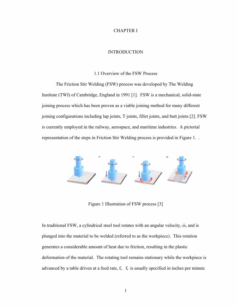
representation of the steps in Friction Stir Welding process is provided in Figure 1. .
Figure 1 Illustration of FSW process [3]
In traditional FSW, a cylindrical steel tool rotates with an angular velocity, ώ, and is
plunged into the material to be welded (referred to as the workpiece). This rotation
generates a considerable amount of heat due to friction, resulting in the plastic
deformation of the material. The rotating tool remains stationary while the workpiece is
advanced by a table driven at a feed rate, fr. fr is usually specified in inches per minute
1
(ipm), while ώ has units of revolutions per minute (rpm). During an FSW process, the
forces in the x, y, and z directions as well as the moment about the z axis are recorded.
Fx is the translational force, Fy is the transverse force, and Fz is the axial force. Forces are
measured in Newtons; the moment is in units of Newton-meters.
Friction Stir Welding has several distinct advantages over traditional arc welding.
FSW generates no fumes, results in reduced distortion and improved weld quality for the
proper parameters, is adaptable to all positions, and is relatively quiet. The major
variables of interest in any FSW process are rotation (spindle) speed, travel speed (feed
rate), tool orientation/position (tilt angle), plunge depth, tool material, tool geometry, and
workpiece material [2].
1.2 FSW Tools
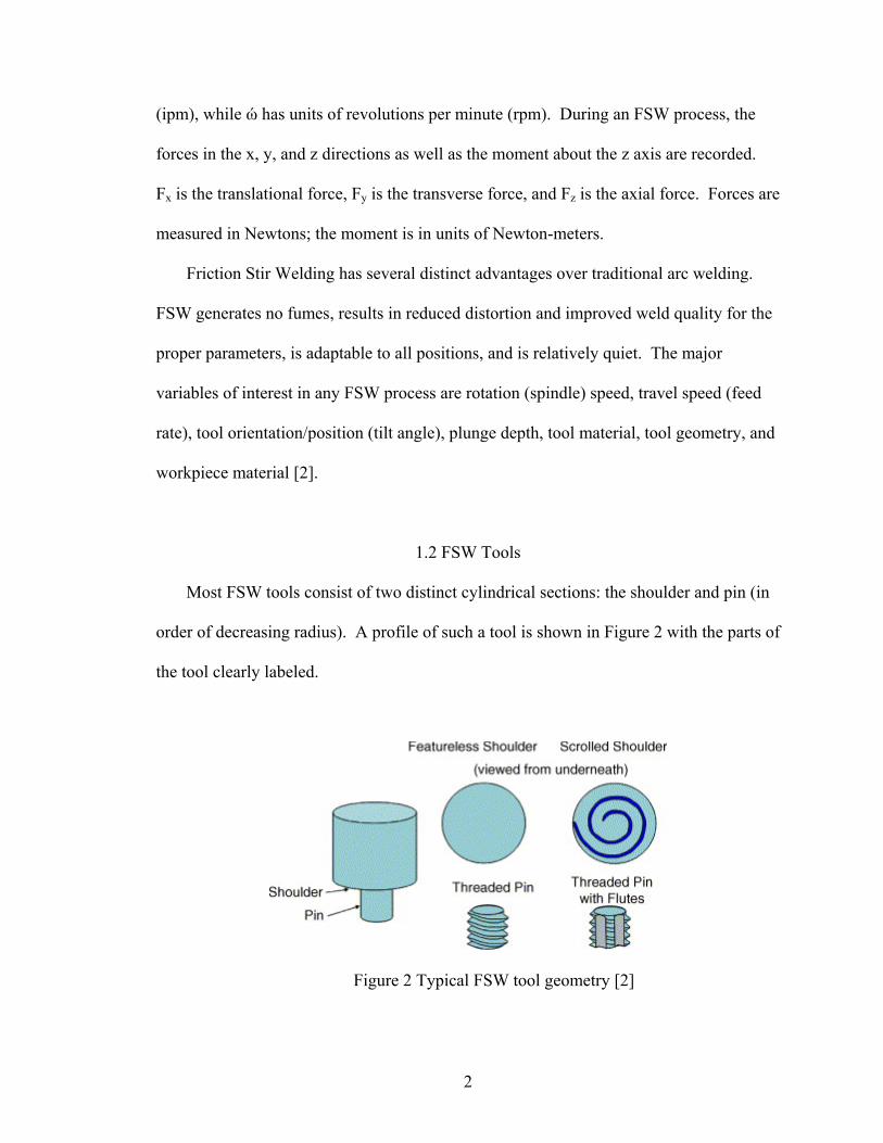
Most FSW tools consist of two distinct cylindrical sections: the shoulder and pin (in
order of decreasing radius). A profile of such a tool is shown in Figure 2 with the parts of
the tool clearly labeled.
Figure 2 Typical FSW tool geometry [2]
2
The pin is plunged into the workpiece and the shoulder maintains contact with the
workpiece surface. This shoulder contact functions to generate frictional heat as the pin
“stirs” the material to be welded [2]. The shape, material, and structure of the FSW tool
is dictated by the workpiece material, the desired quality of the weld, and the rotation
and/or traversing speed. The geometry of the pin may be cylindrical, square, or even
conical. Additionally, threads (similar to those found on a screw) may be machined into
the pin to better facilitate material flow and prevent the formation of wormholes and
other weld defects. In the welding of Aluminum or Aluminum alloys, the most common
choice of tool material is steel: at the proper parameters, it produces good quality, robust
welds and the tool has a slow wear rate. However, if a steel tool is used to weld more
abrasive materials such as Metal Matrix Composites, tool wear becomes a significant
issue due to the presence of abrasive particles and the strength of the material to be
welded [2]. Tools made of more exotic materials such as Molybdenum (Mo), Tungsten
(W), and Tungsten Carbide (WC) can be implemented to reduce or eliminate the tool
wear and distortion which is common in steel tools at high forces and/or rotation speeds.
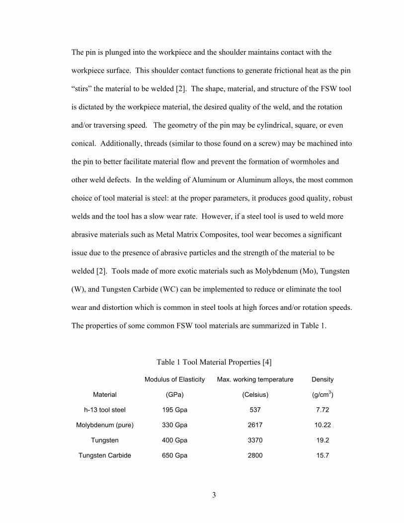
The properties of some common FSW tool materials are summarized in Table 1.
Table 1 Tool Material Properties [4]
Material
Modulus of Elasticity
(GPa)
Max. working temperature
(Celsius)
Density
(g/cm3)
h-13 tool steel 195 Gpa 537 7.72
Molybdenum (pure) 330 Gpa 2617 10.22
Tungsten 400 Gpa 3370 19.2
Tungsten Carbide 650 Gpa 2800 15.7
3
The VU Welding Laboratory currently has tools of Molybdenum and h-13 steel. These
are the base tool materials which will be considered in the subsequent investigation.
1.3 FSW Workpieces with Emphasis on Metal Matrix Composites (MMCs)
Currently, our laboratory work is exclusively concerned with the joining of
Aluminum alloys in a flat plate configuration. This includes butt welds, lap welds, and
T-joint welds. As previously discussed, steel tools with cylindrical geometries are
sufficient for this work. An emerging area of FSW research is the welding of Metal
Matrix Composites (MMCs). The structure of MMCs as well as the particular issues that
arise when joining these materials will now be discussed in detail.
Aluminum Metal Matrix Composites (Al-MMCs) are used in many naval, military,
and aerospace structures. A MMC material is comprised of two parts: a continuous metal
matrix (the material in larger abundance, usually Aluminum) and the reinforcing particles
dispersed throughout the matrix (typically SiC or B4C in concentrations of 10-30%).
Examples of MMCs with industrial applications are 6061/Al2O3/10w , 2618/ Al2O3/15w,
7075/ Al2O3/15w, 2124/SiC/25p, and 6092/SiC/17.5p. Al-MMCs are categorized
according to a classification scheme developed by the Aluminum Association [5]. For
instance, in 7075/ Al2O3/15w, 7075 indicates that the matrix is 7075 Aluminum, the Al2O3
designates that the reinforcement is Aluminum (III) Oxide, and the 15 specifies the
percent of reinforcement present in the material. The p or w subscript indicates the form
of the reinforcement; p corresponds to particulate, while w corresponds to whiskers [5].
4
The high-strength properties associated with MMCs make them difficult to join and
are a limiting factor in the consideration of possible processes. Friction Stir Welding
(FSW) has not traditionally been used for MMC welds because the strength and structure
of the material results in significant tool wear and distortion in the finished weld
(particularly in the heat-affected zone). Since the density of the reinforcement differs
from the density of the matrix material (ex. ρAl = 2.7 g/cm3 < ρSiC = 3.2 g/cm3), the
particles may tend to separate from one another during welding, resulting in
inconsistencies within the finished weld [2]. This is referred to as macrosegregation.
This is undesirable because it can lead to an unfavorable stress distribution in the weld,
possibly resulting in structural deficiency or even failure. The high strength to weight
ratio of MMCs and their resistance to wear, properties which make them attractive for
structural applications, also make them difficult to join. When an MMC is welded using
a standard steel tool, the result is usually excessive tool wear, cracking, and poor weld
quality. Al-MMCs with high reinforcement percentages (greater than thirty percent)
exhibit behavior typical of ceramics, making the welding of joints with these materials
particularly difficult [2].
Friction Stir Welding (FSW) may prove a viable alternative to standard fusion
welding of MMCs. Characteristics of MMC joints welded using fusion techniques such
as TIG welding are usually characterized by incomplete mixing, porosity, and the
presence of a Al4C3 phase. Previous studies of joining the MMCs 6092Al-SiC, A339-
SiC, 6061Al-Al203, and 7093Al-SiC have demonstrated the high-quality welds can be
produced using FSW, but in order for the process to be used on a large scale some
mechanism must be developed to combat the problem of tool wear [2]. A study by
5
Nelson reports that even for an h13 steel tool heat treated to 52 on the Rockwell hardness
scale, the tool wear is so dramatic that no threads are left after only 254 mm (ten inches)
of weld [6]. The mechanism proposed in this study to reduce the aforementioned
problem of tool wear is the use of a Molydenum tool coated with diamond by a Chemical
Vapor Deposition (CVD) method. Previous work on FSW tool coatings and FSW of
MMCs will be examined in the literature review of chapter II.
1.4 Diamond Coating by CVD (Chemical Vapor Deposition)
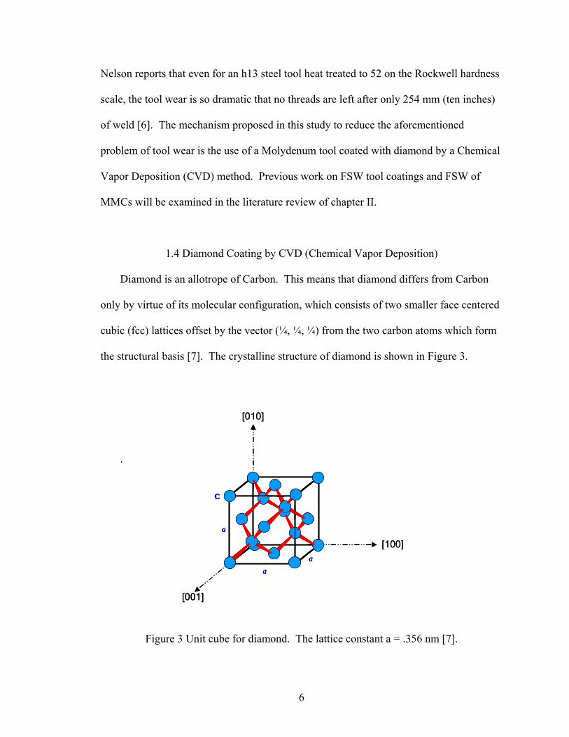
Diamond is an allotrope of Carbon. This means that diamond differs from Carbon
only by virtue of its molecular configuration, which consists of two smaller face centered
cubic (fcc) lattices offset by the vector (¼, ¼, ¼) from the two carbon atoms which form
the structural basis [7]. The crystalline structure of diamond is shown in Figure 3.
a
C
a
a
a
C
a
a
[010]
[001]
[100]
a
C
a
a
a
C
a
a
[010]
[001]
[100]
.
Figure 3 Unit cube for diamond. The lattice constant a = .356 nm [7].
6
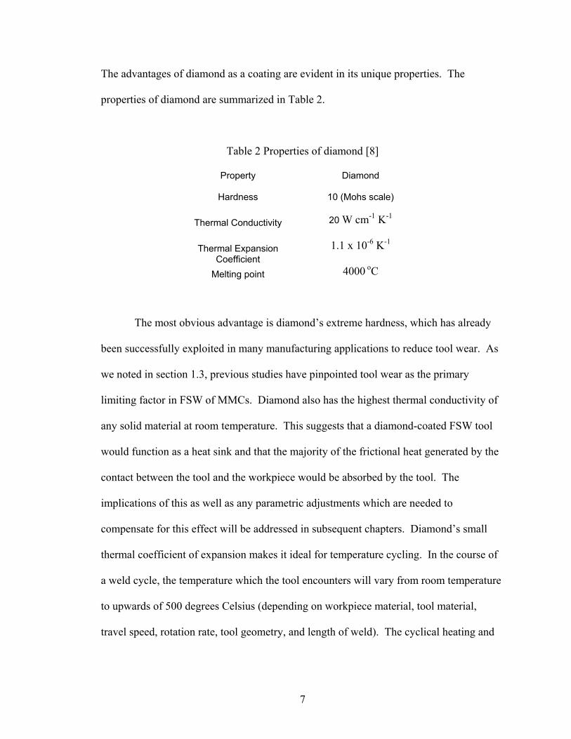
The advantages of diamond as a coating are evident in its unique properties. The
properties of diamond are summarized in Table 2.
Table 2 Properties of diamond [8]
Property Diamond
Hardness 10 (Mohs scale)
Thermal Conductivity 20 W cm-1 K-1
Thermal Expansion Coefficient
1.1 x 10⁻⁶ K-1
Melting point 4000 oC
The most obvious advantage is diamond’s extreme hardness, which has already
been successfully exploited in many manufacturing applications to reduce tool wear. As
we noted in section 1.3, previous studies have pinpointed tool wear as the primary
limiting factor in FSW of MMCs. Diamond also has the highest thermal conductivity of
any solid material at room temperature. This suggests that a diamond-coated FSW tool
would function as a heat sink and that the majority of the frictional heat generated by the
contact between the tool and the workpiece would be absorbed by the tool. The
implications of this as well as any parametric adjustments which are needed to
compensate for this effect will be addressed in subsequent chapters. Diamond’s small
thermal coefficient of expansion makes it ideal for temperature cycling. In the course of
a weld cycle, the temperature which the tool encounters will vary from room temperature
to upwards of 500 degrees Celsius (depending on workpiece material, tool material,
travel speed, rotation rate, tool geometry, and length of weld). The cyclical heating and
7
cooling of the tool which occurs with each weld make coatings with low thermal
expansion coefficients (such as diamond) good candidates for FSW applications.
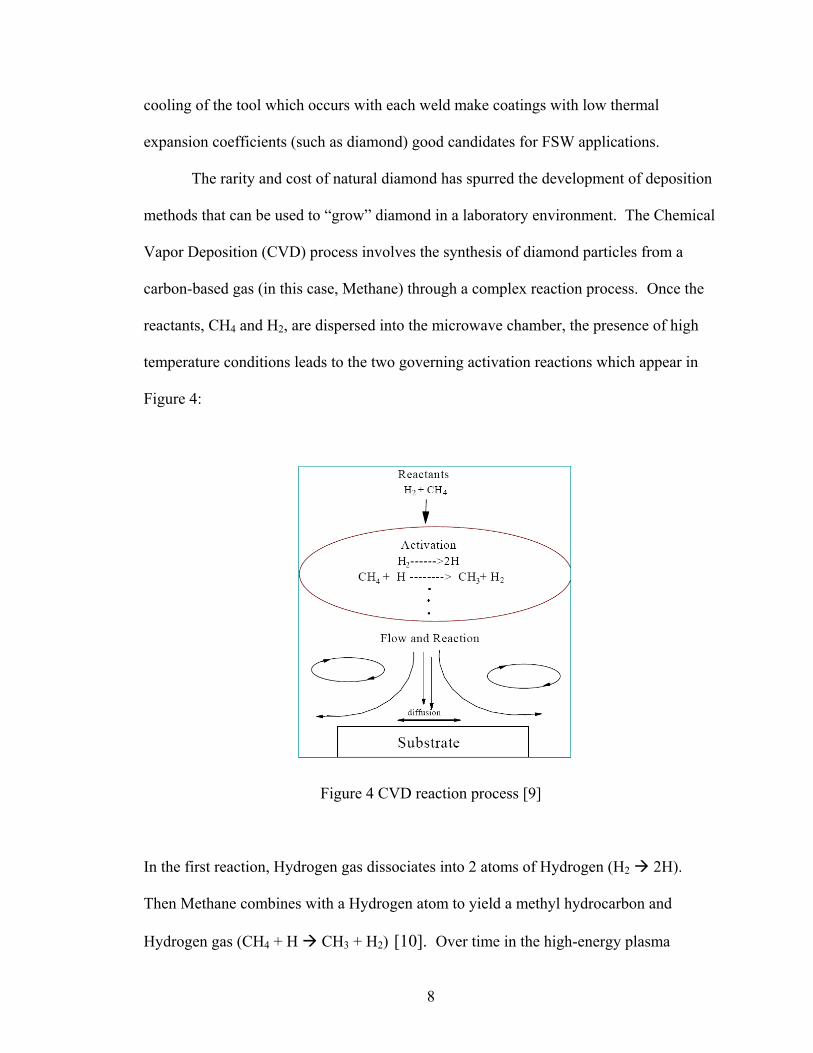
The rarity and cost of natural diamond has spurred the development of deposition
methods that can be used to “grow” diamond in a laboratory environment. The Chemical
Vapor Deposition (CVD) process involves the synthesis of diamond particles from a
carbon-based gas (in this case, Methane) through a complex reaction process. Once the
reactants, CH4 and H2, are dispersed into the microwave chamber, the presence of high
temperature conditions leads to the two governing activation reactions which appear in
Figure 4:
Figure 4 CVD reaction process [9]
In the first reaction, Hydrogen gas dissociates into 2 atoms of Hydrogen (H2 2H).
Then Methane combines with a Hydrogen atom to yield a methyl hydrocarbon and
Hydrogen gas (CH4 + H CH3 + H2) [10]. Over time in the high-energy plasma
8
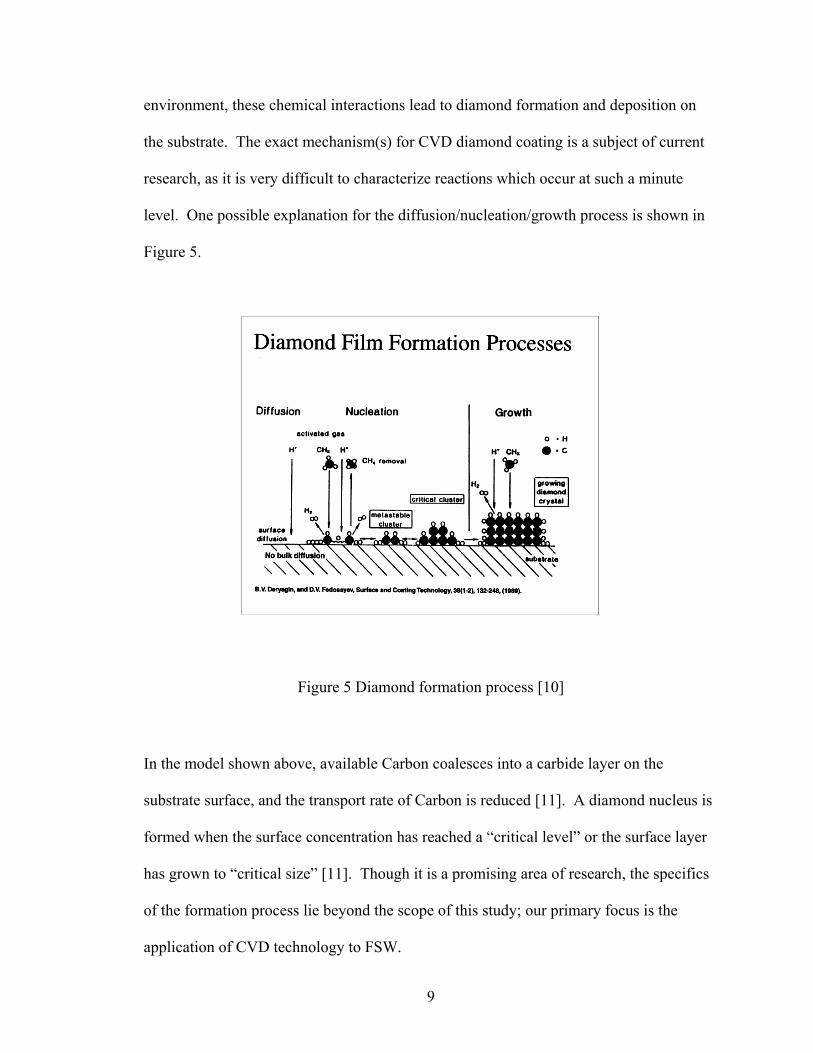
environment, these chemical interactions lead to diamond formation and deposition on
the substrate. The exact mechanism(s) for CVD diamond coating is a subject of current
research, as it is very difficult to characterize reactions which occur at such a minute
level. One possible explanation for the diffusion/nucleation/growth process is shown in
Figure 5.
Figure 5 Diamond formation process [10]
In the model shown above, available Carbon coalesces into a carbide layer on the
substrate surface, and the transport rate of Carbon is reduced [11]. A diamond nucleus is
formed when the surface concentration has reached a “critical level” or the surface layer
has grown to “critical size” [11]. Though it is a promising area of research, the specifics
of the formation process lie beyond the scope of this study; our primary focus is the
application of CVD technology to FSW.
9
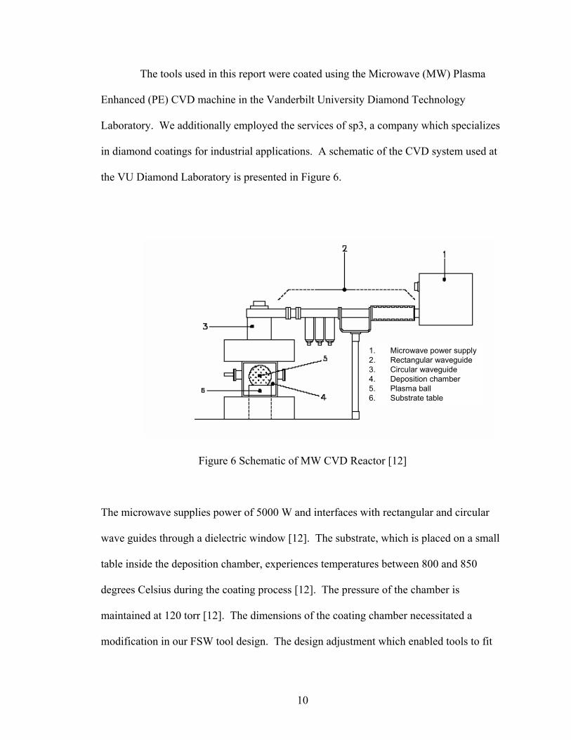
The tools used in this report were coated using the Microwave (MW) Plasma
Enhanced (PE) CVD machine in the Vanderbilt University Diamond Technology
Laboratory. We additionally employed the services of sp3, a company which specializes
in diamond coatings for industrial applications. A schematic of the CVD system used at
the VU Diamond Laboratory is presented in Figure 6.
1. Microwave power supply2. Rectangular waveguide3. Circular waveguide4. Deposition chamber5. Plasma ball6. Substrate table
1. Microwave power supply2. Rectangular waveguide3. Circular waveguide4. Deposition chamber5. Plasma ball6. Substrate table
Figure 6 Schematic of MW CVD Reactor [12]
The microwave supplies power of 5000 W and interfaces with rectangular and circular
wave guides through a dielectric window [12]. The substrate, which is placed on a small
table inside the deposition chamber, experiences temperatures between 800 and 850
degrees Celsius during the coating process [12]. The pressure of the chamber is
maintained at 120 torr [12]. The dimensions of the coating chamber necessitated a
modification in our FSW tool design. The design adjustment which enabled tools to fit
10
inside the chamber for coating will be discussed at length in the chapter on experimental
setup.
Additionally, the harsh environment of the deposition chamber imposes specific
demands on the choice of substrate material. The substrate must be able to not just
withstand the high temperatures and pressure associated with the coating process, but to
do so without compromising the integrity of the base material. An ideal substrate
candidate does not contain carbon (thus eliminating the potential of carbon carbon
interaction) and has a coefficient of thermal expansion comparable to that of diamond
[13]. The choice of substrate is critical: the quality of the resultant coating depends
largely on the properties of the substrate itself.
1.5 Microstructural Zones
A typical FSW weld produces four distinct microstructural zones: the heat-
affected zone (HAZ), the thermal mechanically affected zone (TMAZ), the weld nugget,
and the unaffected zone (also known as parent material). The unaffected zone is exactly
what its name implies: the material in this region is unaffected by the joining process and
thus retains the mechanical properties associated with the workpiece material. The HAZ
is characterized by a change in the microstructure due to heating and plastic deformation.
The TMAZ is the site of plastic deformation. The weld nugget is the region of the weld
in which the pin contacts the workpiece and thus is the area in which heat and plastic
deformation are most pronounced. The weld nugget is also a site of recrystallization. A
visual representation of the four weld zones appears in Figure 7.
11
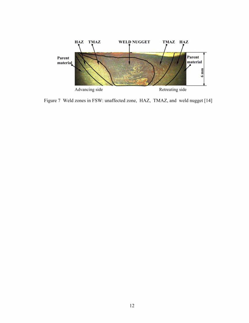
Figure 7 Weld zones in FSW: unaffected zone, HAZ, TMAZ, and weld nugget [14]
12
CHAPTER II
LITERATURE REVIEW
In this chapter, we will consider previous friction stir welding research on the
parameterization of joining Metal Matrix Composites. Additionally, we will review
studies concerning the use of coatings to reduce tool wear in the welding of superabrasive
materials. Special emphasis is placed on joining Aluminum alloy series MMCs with
varying percentages of SiC reinforcement, since this is the same material that was used in
our research.
The motivation behind investigating friction stir welding as a method for joining
MMCs is explicated in the Storjohann, et al. article “Fusion and Friction Stir Welding of
Aluminum-Metal Matrix Composites,” which provides a full assessment of the problems
inherent in welding MMCs using traditional fusion techniques. Storjohann et al. utilize
three different fusion methods to weld Aluminum composites reinforced with SiC
whiskers: gas tungsten arc (GTA), electron beam (EB), and Nd-YAG continuous wave
laser beam (LB). The authors compare these welds with those produced using FSW to
determine what effect, if any, the solid state method has on weld quality. As noted in the
literature pertaining to joining MMCs, the problem with fusion methods lies in the
formation of an Al4C3 phase as a result of the interaction between the SiC reinforcement
and molten aluminum. The authors postulate that the amount of Al4C3 present in a
resultant weld is closely related to the peak weld temperature (i.e. a higher temperature
produces a greater abundance of Al4C3). Since FSW is a lower temperature process that
13

does not melt the workpiece material, it is hypothesized that the FSW welds will have a
smaller concentration of the deleterious Aluminum Carbide phase [15]. The materials
Storjohann et al. used in his paper were 4 mm (approximately 5/32”) thick plates of
Aluminum 2124 alloy with twenty percent SiC whisker reinforcement. The heat input
per unit length (referred to as the energy density) was 4200 J/in for GTA, 150 J/in for EB,
and 2750 J/in for LB. The FSW parameters were a rotation speed of 500 RPM and a
travel speed of 2 ipm. In analyzing the welds, the authors were primarily concerned with
how the joining process would affect the orientation of the SiC reinforcements. It is their
belief that favorable mechanical properties in the finished joint are largely dependent
upon the post-weld distribution of the reinforcement particles.
In microstructural analyses of the fusion welds, Storjohann, et al. observe varying
degrees of porosity in the HAZ region for all three methods. These porosities exhibit
elongation in the x-direction, which the authors attribute to the tensile stresses the
particles are subjected to during the weld cycle. In the fusion zone (FZ), there is
complete dissolution of the SiC whiskers due to heating. The authors conclude that the
formation of the Al4C3 phase is an inevitable consequence of fusion welding. The effect
can be minimized by the careful control of heat input, but even the process with the
lowest heat input per unit length (EB) shows evidence of Al4C3. The optical
micrographs which appear in Figure 8 demonstrate the degree to which the Al4C3 phase
occurs in the fusion welding processes considered by Storjohann, et al. It should be
noted that even though the LB process has a smaller heat input than GTA, there is greater
penetration due to the high laser absorption coefficient of the SiC whiskers.
14
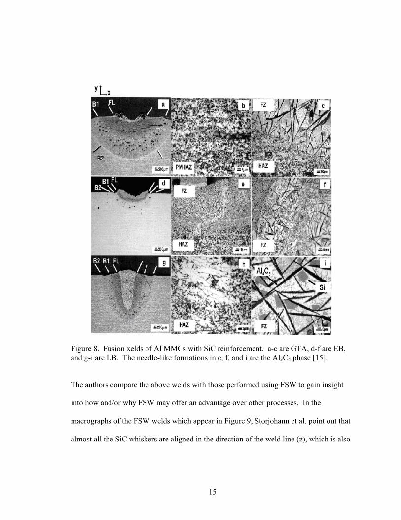
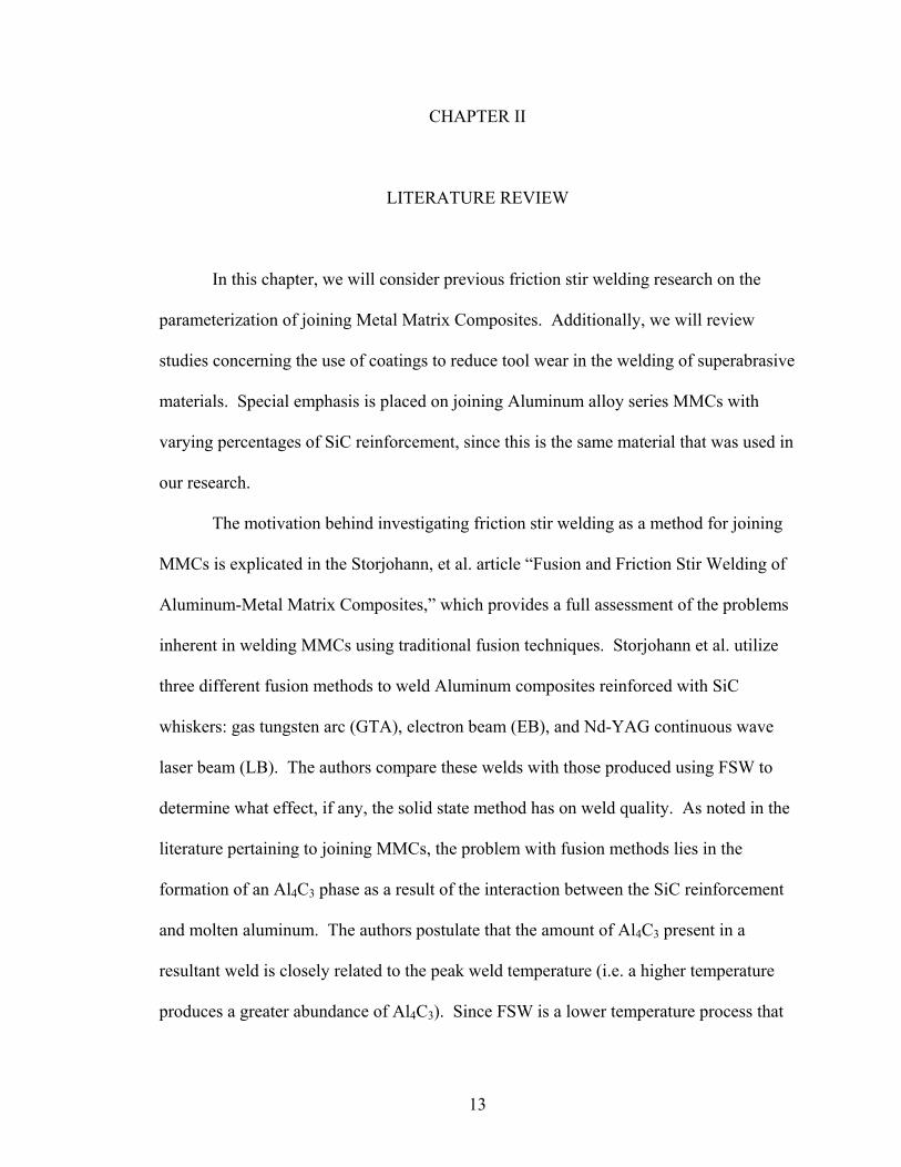
Figure 8. Fusion xelds of Al MMCs with SiC reinforcement. a-c are GTA, d-f are EB, and g-i are LB. The needle-like formations in c, f, and i are the Al3C4 phase [15]. The authors compare the above welds with those performed using FSW to gain insight
into how and/or why FSW may offer an advantage over other processes. In the
macrographs of the FSW welds which appear in Figure 9, Storjohann et al. point out that
almost all the SiC whiskers are aligned in the direction of the weld line (z), which is also
15
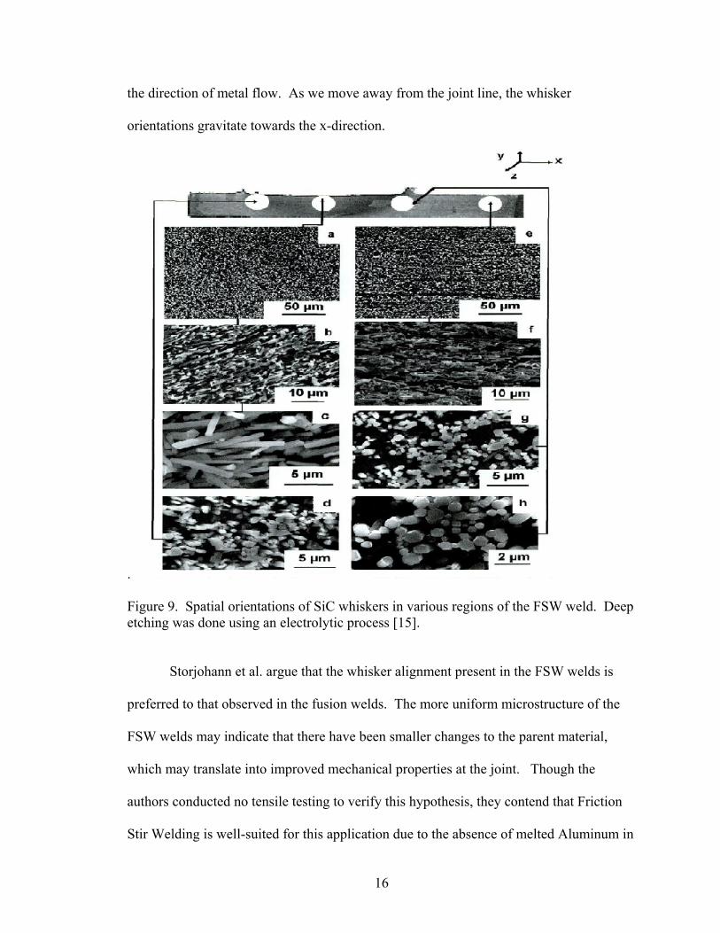
the direction of metal flow. As we move away from the joint line, the whisker
orientations gravitate towards the x-direction.
.
Figure 9. Spatial orientations of SiC whiskers in various regions of the FSW weld. Deep etching was done using an electrolytic process [15].
Storjohann et al. argue that the whisker alignment present in the FSW welds is
preferred to that observed in the fusion welds. The more uniform microstructure of the
FSW welds may indicate that there have been smaller changes to the parent material,
which may translate into improved mechanical properties at the joint. Though the
authors conducted no tensile testing to verify this hypothesis, they contend that Friction
Stir Welding is well-suited for this application due to the absence of melted Aluminum in
16
the weld, which reacts with SiC in fusion welds to form the Al4C3 phase. Though work
by Ellis has demonstrated that the formation of Al4C3 can be avoided in GTA welds, it
requires careful control of the energy density [15]. Similarly, a study by Dahotre, et al.
indicates that pulsing in laser welds reduces the accumulation of Al4C3 [16]. We should
note that the Al4C3 phase is still observed in FSW welds of Al-MMCs, albeit it in
significantly smaller quantities than in fusion welds. The degree to which this deleterious
phase affects FSW joint properties is an area of current research.
In related research, Storjohann, et al. attempt to quantify the amount of Al4C3
formed as a function of weld temperature. They conclude that as the temperature
increases and/or exceeds the melting point of the Aluminum, the reaction which
transforms SiC into Al4C3 increases in rate. For this reason, it is desirable to keep the
temperature of the workpiece below the melting point. This explains Storjohann’s et al.
previous assertion that solid state welding processes have great potential to lessen (or in
some cases eliminate) the presence of Al4C3 in the completed joint.
The Storjohann paper, with its emphasis on Al4C3, establishes the motivation
behind using FSW to join MMCs. The earliest feasibility studies on FSW of Aluminum
MMCs with SiC reinforcements were conducted at NASA’s Marshall Space Flight
Center (MSFC) in the late 1990s. In a technical memorandum entitled “Friction Stir
Welding for Aluminum Metal Matrix Composites” from 1999, Lee et al. assess using
FSW to weld Aluminum MMCs reinforced with varying percentages of discontinuous
SiC particulate (as opposed to the whisker reinforcements used in the Storjohann paper)
[17]. Lee et al. reiterate the advantages FSW may offer for this application, placing
particular emphasis on lower thermal energy requirements and the absence of undesirable
17
chemical reactions. Additionally, Lee points out that the FSW process is much less
reliant on human/operator expertise than fusion methods such as GTA [17].
The NASA investigation used FSW tools with a 0.475” diameter shoulder and a
0.120” long pin with 10-24 left handed threads, whose dimensions were based on the
results of computer simulations. These tools were used to weld flat-plate configurations
of specimens measuring 0.125” in thickness. It is unusual for researchers to divulge tool
geometry in publications, as this is often considered proprietary information and is
closely guarded by the company or organization sponsoring the research. The tool for
this report, however, was independently designed by the co-author, so disclosure is not an
issue in this instance.
Since the authors anticipated tool wear in welding MMCs, the performance of
tools made of h-13 steel hardened to 55 on the Rockwell Hardness scale were compared
against tools of identical geometry coated with B4C, a material which has a hardness
value slightly less than that of diamond. The tools were used to perform butt welds of
6092 Aluminum alloy with 17.5 percent SiC particle reinforcement. The properties of
this material, which are comparable to those of the MMCs used in our own investigation,
are summarized in Table 3.
18
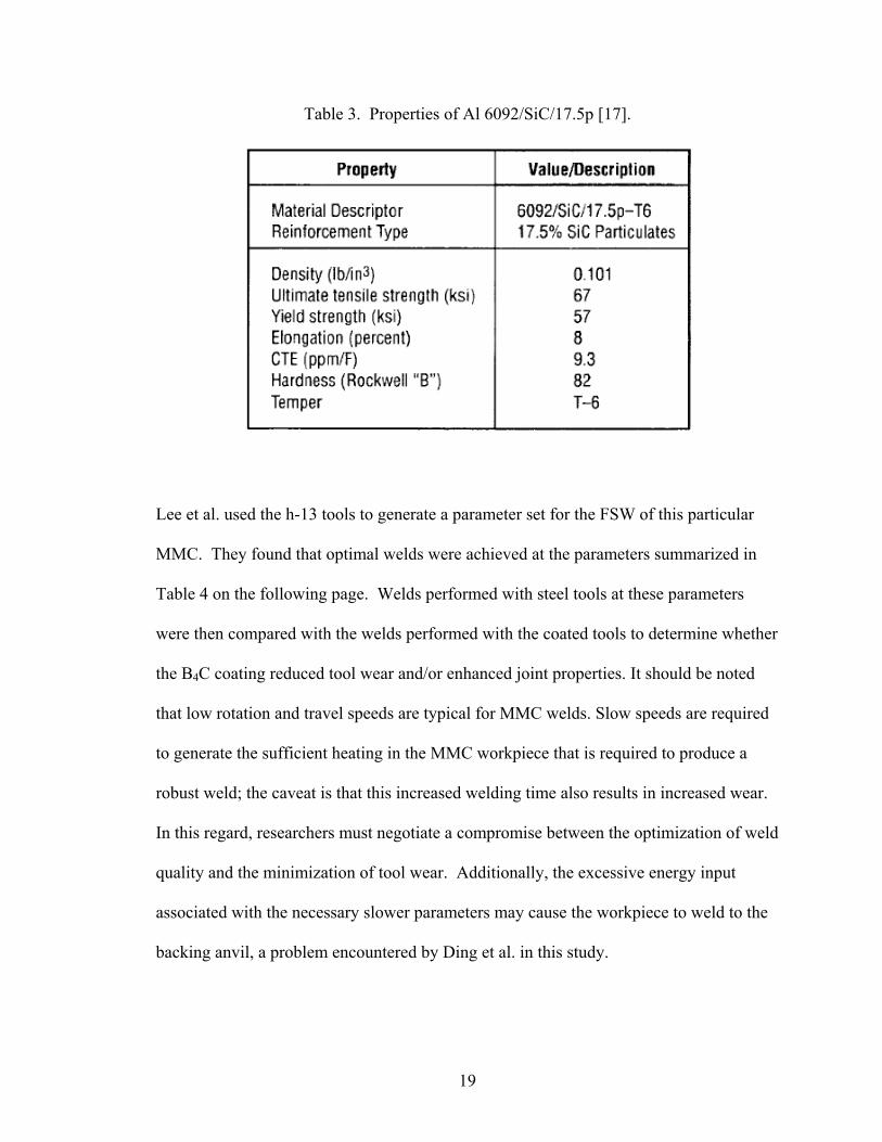
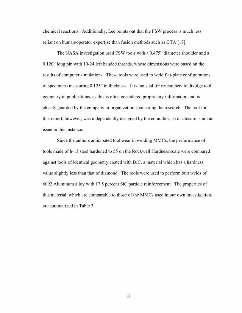
Table 3. Properties of Al 6092/SiC/17.5p [17].
Lee et al. used the h-13 tools to generate a parameter set for the FSW of this particular
MMC. They found that optimal welds were achieved at the parameters summarized in
Table 4 on the following page. Welds performed with steel tools at these parameters
were then compared with the welds performed with the coated tools to determine whether
the B4C coating reduced tool wear and/or enhanced joint properties. It should be noted
that low rotation and travel speeds are typical for MMC welds. Slow speeds are required
to generate the sufficient heating in the MMC workpiece that is required to produce a
robust weld; the caveat is that this increased welding time also results in increased wear.
In this regard, researchers must negotiate a compromise between the optimization of weld
quality and the minimization of tool wear. Additionally, the excessive energy input
associated with the necessary slower parameters may cause the workpiece to weld to the
backing anvil, a problem encountered by Ding et al. in this study.
19
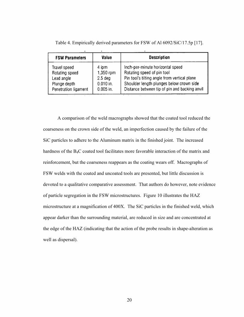
Table 4. Empirically derived parameters for FSW of Al 6092/SiC/17.5p [17].
A comparison of the weld macrographs showed that the coated tool reduced the
coarseness on the crown side of the weld, an imperfection caused by the failure of the
SiC particles to adhere to the Aluminum matrix in the finished joint. The increased
hardness of the B4C coated tool facilitates more favorable interaction of the matrix and
reinforcement, but the coarseness reappears as the coating wears off. Macrographs of
FSW welds with the coated and uncoated tools are presented, but little discussion is
devoted to a qualitative comparative assessment. That authors do however, note evidence
of particle segregation in the FSW microstructures. Figure 10 illustrates the HAZ
microstructure at a magnification of 400X. The SiC particles in the finished weld, which
appear darker than the surrounding material, are reduced in size and are concentrated at
the edge of the HAZ (indicating that the action of the probe results in shape-alteration as
well as dispersal).
20
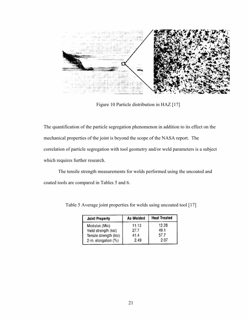
Figure 10 Particle distribution in HAZ [17]
The quantification of the particle segregation phenomenon in addition to its effect on the
mechanical properties of the joint is beyond the scope of the NASA report. The
correlation of particle segregation with tool geometry and/or weld parameters is a subject
which requires further research.
The tensile strength measurements for welds performed using the uncoated and
coated tools are compared in Tables 5 and 6.
Table 5 Average joint properties for welds using uncoated tool [17]
21
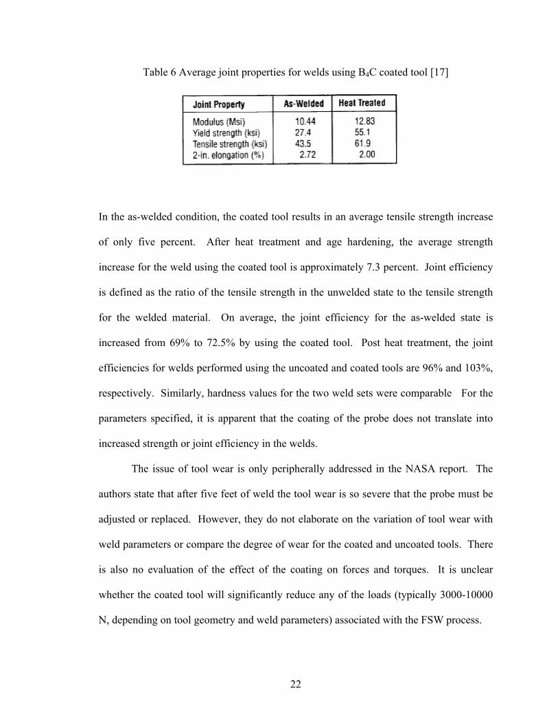
Table 6 Average joint properties for welds using B4C coated tool [17]
In the as-welded condition, the coated tool results in an average tensile strength increase
of only five percent. After heat treatment and age hardening, the average strength
increase for the weld using the coated tool is approximately 7.3 percent. Joint efficiency
is defined as the ratio of the tensile strength in the unwelded state to the tensile strength
for the welded material. On average, the joint efficiency for the as-welded state is
increased from 69% to 72.5% by using the coated tool. Post heat treatment, the joint
efficiencies for welds performed using the uncoated and coated tools are 96% and 103%,
respectively. Similarly, hardness values for the two weld sets were comparable For the
parameters specified, it is apparent that the coating of the probe does not translate into
increased strength or joint efficiency in the welds.
The issue of tool wear is only peripherally addressed in the NASA report. The
authors state that after five feet of weld the tool wear is so severe that the probe must be
adjusted or replaced. However, they do not elaborate on the variation of tool wear with
weld parameters or compare the degree of wear for the coated and uncoated tools. There
is also no evaluation of the effect of the coating on forces and torques. It is unclear
whether the coated tool will significantly reduce any of the loads (typically 3000-10000
N, depending on tool geometry and weld parameters) associated with the FSW process.
22
The remainder of the NASA report focuses on the FSW of functionally gradient
Al MMC to another composite, Al-Li 2195. Though the application for the work is never
explicitly stated, the research may be related to the manufacturing of the architecture for
the Constellation program, which requires circumferential joining of Al-Li 2195
composites by FSW methods. A functionally gradient material (FGM) is an MMC which
has a high percentage reinforcement (often upwards of 50 percent) in the center of the
plate, but significantly less near the weld line. The thickness of the FGM was 0.25 inches
for all welds. All Al-MMC FGMs had a 50% SiC reinforcement at the center, but the
percentage reinforcement at the edge varied from 5 to 50 percent. The Al-MMC FGMs
were butt welded to Al-Li 2195 using a threaded probe with length 0.230 in and shoulder
diameter 0.738 in [17]. The materials tested, weld parameters, and results are
summarized in Table 7. The authors postulate that the probe breaks in the materials with
higher levels of reinforcement at the edge may be due to extreme forces encountered
during the course of the weld. These excessive forces can be attributed to the disparities
in temperature and conductivity between the Al MMC FGM and the Al-Li 2195
composite
.
23
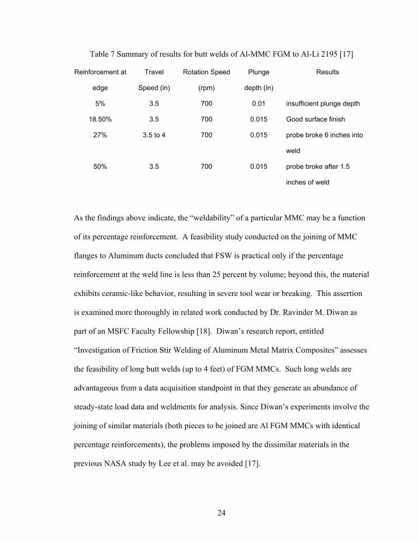
Table 7 Summary of results for butt welds of Al-MMC FGM to Al-Li 2195 [17]
Reinforcement at
edge
Travel
Speed (in)
Rotation Speed
(rpm)
Plunge
depth (in)
Results
5% 3.5 700 0.01 insufficient plunge depth
18.50% 3.5 700 0.015 Good surface finish
27% 3.5 to 4 700 0.015 probe broke 6 inches into
weld
50% 3.5 700 0.015 probe broke after 1.5
inches of weld
As the findings above indicate, the “weldability” of a particular MMC may be a function
of its percentage reinforcement. A feasibility study conducted on the joining of MMC
flanges to Aluminum ducts concluded that FSW is practical only if the percentage
reinforcement at the weld line is less than 25 percent by volume; beyond this, the material
exhibits ceramic-like behavior, resulting in severe tool wear or breaking. This assertion
is examined more thoroughly in related work conducted by Dr. Ravinder M. Diwan as
part of an MSFC Faculty Fellowship [18]. Diwan’s research report, entitled
“Investigation of Friction Stir Welding of Aluminum Metal Matrix Composites” assesses
the feasibility of long butt welds (up to 4 feet) of FGM MMCs. Such long welds are
advantageous from a data acquisition standpoint in that they generate an abundance of
steady-state load data and weldments for analysis. Since Diwan’s experiments involve the
joining of similar materials (both pieces to be joined are Al FGM MMCs with identical
percentage reinforcements), the problems imposed by the dissimilar materials in the
previous NASA study by Lee et al. may be avoided [17].
24
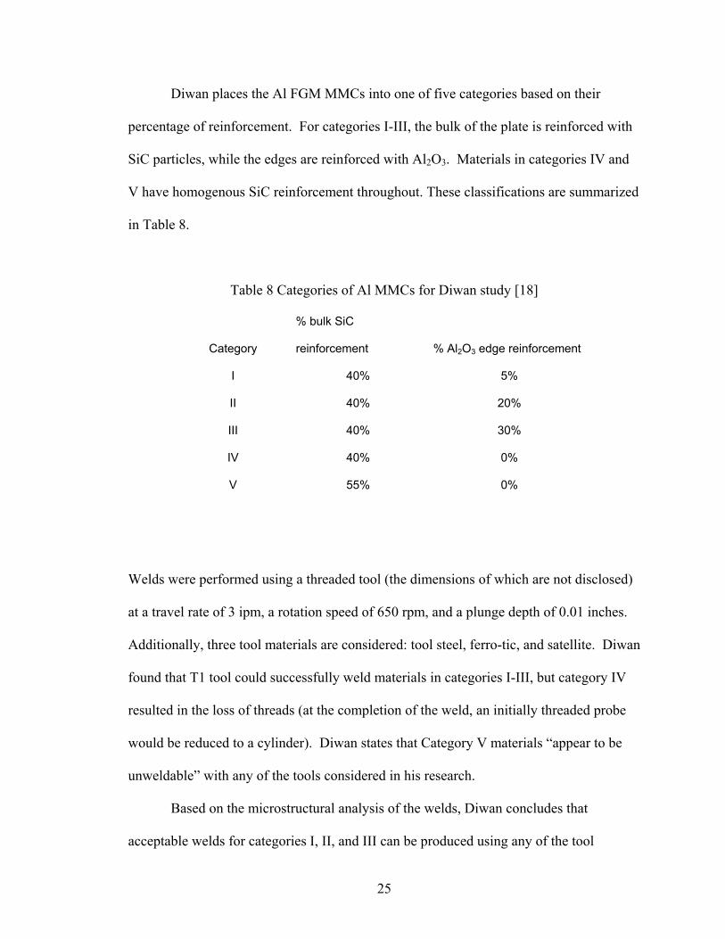
Diwan places the Al FGM MMCs into one of five categories based on their
percentage of reinforcement. For categories I-III, the bulk of the plate is reinforced with
SiC particles, while the edges are reinforced with Al2O3. Materials in categories IV and
V have homogenous SiC reinforcement throughout. These classifications are summarized
in Table 8.
Table 8 Categories of Al MMCs for Diwan study [18]
Category
% bulk SiC
reinforcement % Al2O3 edge reinforcement
I 40% 5%
II 40% 20%
III 40% 30%
IV 40% 0%
V 55% 0%
Welds were performed using a threaded tool (the dimensions of which are not disclosed)
at a travel rate of 3 ipm, a rotation speed of 650 rpm, and a plunge depth of 0.01 inches.
Additionally, three tool materials are considered: tool steel, ferro-tic, and satellite. Diwan
found that T1 tool could successfully weld materials in categories I-III, but category IV
resulted in the loss of threads (at the completion of the weld, an initially threaded probe
would be reduced to a cylinder). Diwan states that Category V materials “appear to be
unweldable” with any of the tools considered in his research.
Based on the microstructural analysis of the welds, Diwan concludes that
acceptable welds for categories I, II, and III can be produced using any of the tool
25
materials considered. Diwan recommends further research into welding optimization of
category I-III materials to reduce and/or eliminate any defects apparent in the
microstructure. Category IV materials pose a significant problem: wear is severe
regardless of the tool material and the probe is prone to break or fracture during the
welding process. Though Diwan’s research is only a broad study of MMC welds (the
specifics of wear and microscopy observed during the investigation are scarce), it does
corroborate the hypothesis that the weldability of an MMC is inversely proportional to its
percentage reinforcement along the weld line. There also appears to be a threshold
(around 50% reinforcement) beyond which MMCs cannot be welded using the proposed
tools.
We now move away from feasibility studies and toward parameterization and the
characterization of microstructural behavior for a range of composite materials. One
such composite material that has been a focus of recent welding research is Al
6061/Al2O3/20p (which was previously considered by Diwan). In the paper “Friction stir
welding of an AA6061/ Al2O3/20p reinforced alloy,” Marzoli et al. establish a working
envelope for this material and assess how joint efficiencies and microstructures are
impacted by the choice of parameters [19]. Marzoli et al. performed FSW butt welds of
the reinforced alloy using a tool with a 0.75” diameter shoulder and 0.3” diameter probe.
The probe length, geometry, and tool material are not specified. The experimental weld
matrix constructed by Marzoli, et al. appears in Figure 11. Spindle speed is plotted on
the y-axis, while travel speed (in mm/min) appears on the x-axis. The blue circles
indicate the parameters which produced a defect-free weld. Note that the operating
window is narrow, including only rotation speeds from 475 rpm to 700 rpm and travel
26
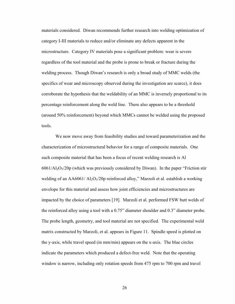
speeds from 150 mm/min (approximately 6 ipm) to 300 mm/min (12 ipm). This welding
envelope of slower parameters is characteristic of composite materials, which require
increased energy input. The triangles represent a “process limit” beyond which not
enough plastic deformation occurs to produce an acceptable weld. The red squares
denote the robotic limits of the welding apparatus.
Figure 11 Welding envelope for 6061/Al2O3/20p [19]
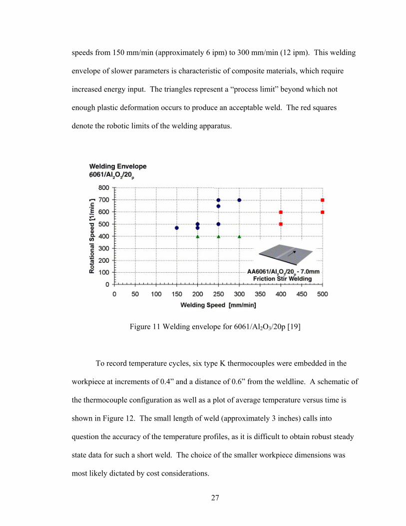
To record temperature cycles, six type K thermocouples were embedded in the
workpiece at increments of 0.4” and a distance of 0.6” from the weldline. A schematic of
the thermocouple configuration as well as a plot of average temperature versus time is
shown in Figure 12. The small length of weld (approximately 3 inches) calls into
question the accuracy of the temperature profiles, as it is difficult to obtain robust steady
state data for such a short weld. The choice of the smaller workpiece dimensions was
most likely dictated by cost considerations.
27
The highest temperature, 250 degrees Celsius, is observed at T1, the
thermocouple positioned closest to the start of the weld. This is because the higher
energy input required to plasticize the material necessitates a gradual increase in welding
speed. For instance, if the steady state travel speed is specified as 5 inches per minute,
the tool will enter the weld at a slightly lower travel rate and “ramp up” to the steady state
value. This is a common experimental technique in FSW and one we employ in our own
laboratory work.
Figure 12 Thermal cycles [19]
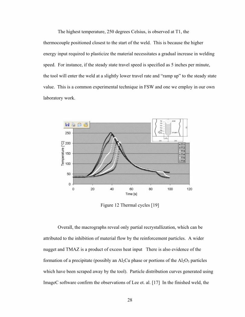
Overall, the macrographs reveal only partial recrystallization, which can be
attributed to the inhibition of material flow by the reinforcement particles. A wider
nugget and TMAZ is a product of excess heat input There is also evidence of the
formation of a precipitate (possibly an Al2Cu phase or portions of the Al2O3 particles
which have been scraped away by the tool). Particle distribution curves generated using
ImageC software confirm the observations of Lee et. al. [17] In the finished weld, the
28
reinforcement particles are smaller and more rounded than in the parent material.
Marzoli postulates that this reduction in particle size which comes about as a result of
friction stir welding may actually function to enhance material properties.
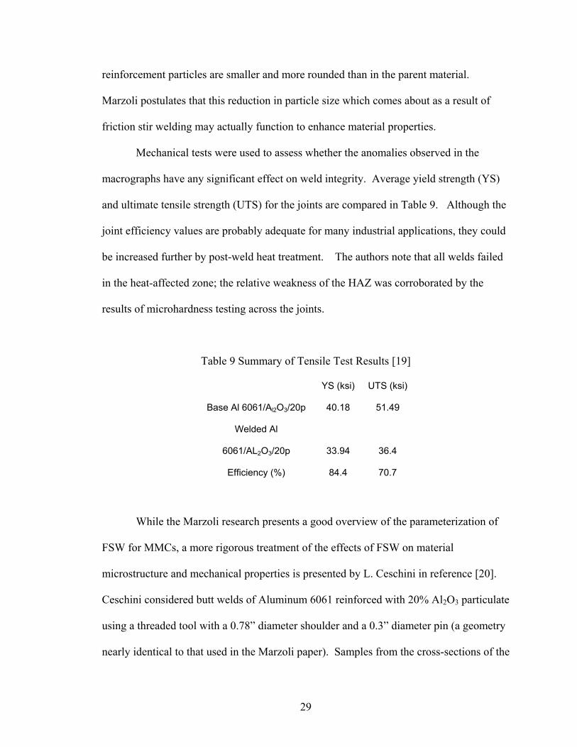
Mechanical tests were used to assess whether the anomalies observed in the
macrographs have any significant effect on weld integrity. Average yield strength (YS)
and ultimate tensile strength (UTS) for the joints are compared in Table 9. Although the
joint efficiency values are probably adequate for many industrial applications, they could
be increased further by post-weld heat treatment. The authors note that all welds failed
in the heat-affected zone; the relative weakness of the HAZ was corroborated by the
results of microhardness testing across the joints.
Table 9 Summary of Tensile Test Results [19]
YS (ksi) UTS (ksi)
Base Al 6061/Al2O3/20p 40.18 51.49
Welded Al
6061/AL2O3/20p 33.94 36.4
Efficiency (%) 84.4 70.7
While the Marzoli research presents a good overview of the parameterization of
FSW for MMCs, a more rigorous treatment of the effects of FSW on material
microstructure and mechanical properties is presented by L. Ceschini in reference [20].
Ceschini considered butt welds of Aluminum 6061 reinforced with 20% Al2O3 particulate
using a threaded tool with a 0.78” diameter shoulder and a 0.3” diameter pin (a geometry
nearly identical to that used in the Marzoli paper). Samples from the cross-sections of the
29
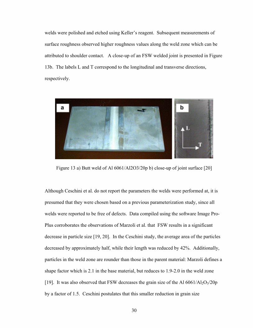
welds were polished and etched using Keller’s reagent. Subsequent measurements of
surface roughness observed higher roughness values along the weld zone which can be
attributed to shoulder contact. A close-up of an FSW welded joint is presented in Figure
13b. The labels L and T correspond to the longitudinal and transverse directions,
respectively.
Figure 13 a) Butt weld of Al 6061/Al2O3/20p b) close-up of joint surface [20]
Although Ceschini et al. do not report the parameters the welds were performed at, it is
presumed that they were chosen based on a previous parameterization study, since all
welds were reported to be free of defects. Data compiled using the software Image Pro-
Plus corroborates the observations of Marzoli et al. that FSW results in a significant
decrease in particle size [19, 20]. In the Ceschini study, the average area of the particles
decreased by approximately half, while their length was reduced by 42%. Additionally,
particles in the weld zone are rounder than those in the parent material: Marzoli defines a
shape factor which is 2.1 in the base material, but reduces to 1.9-2.0 in the weld zone
[19]. It was also observed that FSW decreases the grain size of the Al 6061/Al2O3/20p
by a factor of 1.5. Ceschini postulates that this smaller reduction in grain size
30
(unreinforced Al 6061 experiences a tenfold reduction in grain size after undergoing
FSW) is due to the already fine microstructure of the composite material [20].
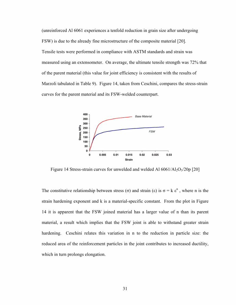
Tensile tests were performed in compliance with ASTM standards and strain was
measured using an extensometer. On average, the ultimate tensile strength was 72% that
of the parent material (this value for joint efficiency is consistent with the results of
Marzoli tabulated in Table 9). Figure 14, taken from Ceschini, compares the stress-strain
curves for the parent material and its FSW-welded counterpart.
Figure 14 Stress-strain curves for unwelded and welded Al 6061/Al2O3/20p [20]
The constitutive relationship between stress (σ) and strain (ε) is σ = k εn , where n is the
strain hardening exponent and k is a material-specific constant. From the plot in Figure
14 it is apparent that the FSW joined material has a larger value of n than its parent
material, a result which implies that the FSW joint is able to withstand greater strain
hardening. Ceschini relates this variation in n to the reduction in particle size: the
reduced area of the reinforcement particles in the joint contributes to increased ductility,
which in turn prolongs elongation.
31
Ceschini also subjected the welded samples to low-cycle fatigue tests. The results
of these tests indicated that fatigue life was reduced in the FSW joints, an outcome that is
consistent with the previous comparison of joint efficiency for the unwelded and welded
samples. For low strain amplitudes, the fatigue life of the base material was twice as long
as that of its FSW counterpart. For high strain amplitudes, the life span of the base
material reached ten times that of the welded joint. Based on the plots of hysteresis loops
at these different strain amplitudes, Ceschini concludes that the FSW composite
undergoes increased plastic strain. He contends that this amplified strain, in conjunction
with the non-homogeneity of the MMC, is responsible for the reduced fatigue life of the
FSW joint.
Ceschini also examined the fracture surfaces after the fatigue tests had been
performed. He proposes that there are three principal causes of fracture in the joint: I)
fissuring of the reinforcement particles, II) desolidification along the particle/matrix
boundaries, and III) void formation and enlargement within the matrix (a result of the
aforementioned desolidification). SEM micrographs reveal that a type I fracture occurs
in areas with larger particles, while distributions of smaller particles along the weld line
primarily produce fractures of types II and III. Ceshini provides qualitative data in the
form of micrographs to substantiate these observations, but does not characterize how
fracture mechanisms are affected by weld parameters or tool geometry.
A comparable evaluation of the fracture behavior of Al 6061/Al2O3/20p is
presented in the Cavliere et al. paper “Friction Stir Welding of Ceramic Particle
Reinforced Aluminum Based Metal Matrix Composites.” Though Cavalierie et. al. opt
not to disclose tool dimensions (for this reason it may be misleading to directly compare
32
their results with those of the Ceschini study), they specify the tool rotation speed as 800
RPM and the travel rate as approximately 2 inches per minute. They record a slightly
higher joint efficiency (84%-87%) than was reported in previous literature; this increased
efficiency may be ascribed to the choice of weld parameters or the (unspecified) tool
geometry used in the study. An examination of the microstructure of the welded samples
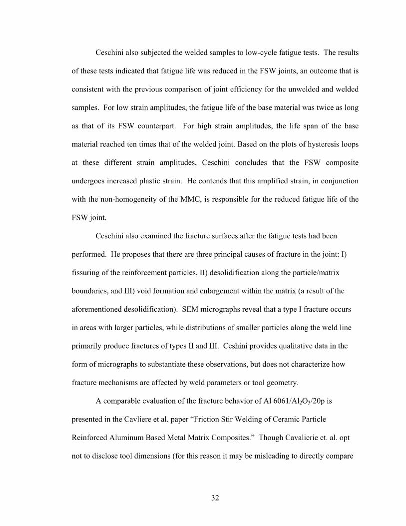
reveals fracture behavior consistent with that characterized by Ceschini in reference [20].
Particle fracture along the matrix/particle interface (Ceshcini’s “type II” fracture) can be
seen clearly in Figure 15.
Figure 15 Particle fracture in FSW Al 6061/Al2O3/20p [21]
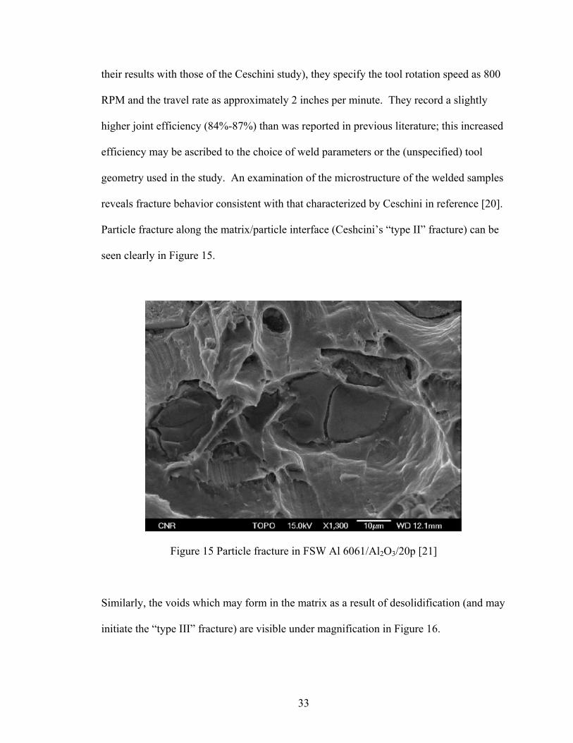
Similarly, the voids which may form in the matrix as a result of desolidification (and may
initiate the “type III” fracture) are visible under magnification in Figure 16.
33
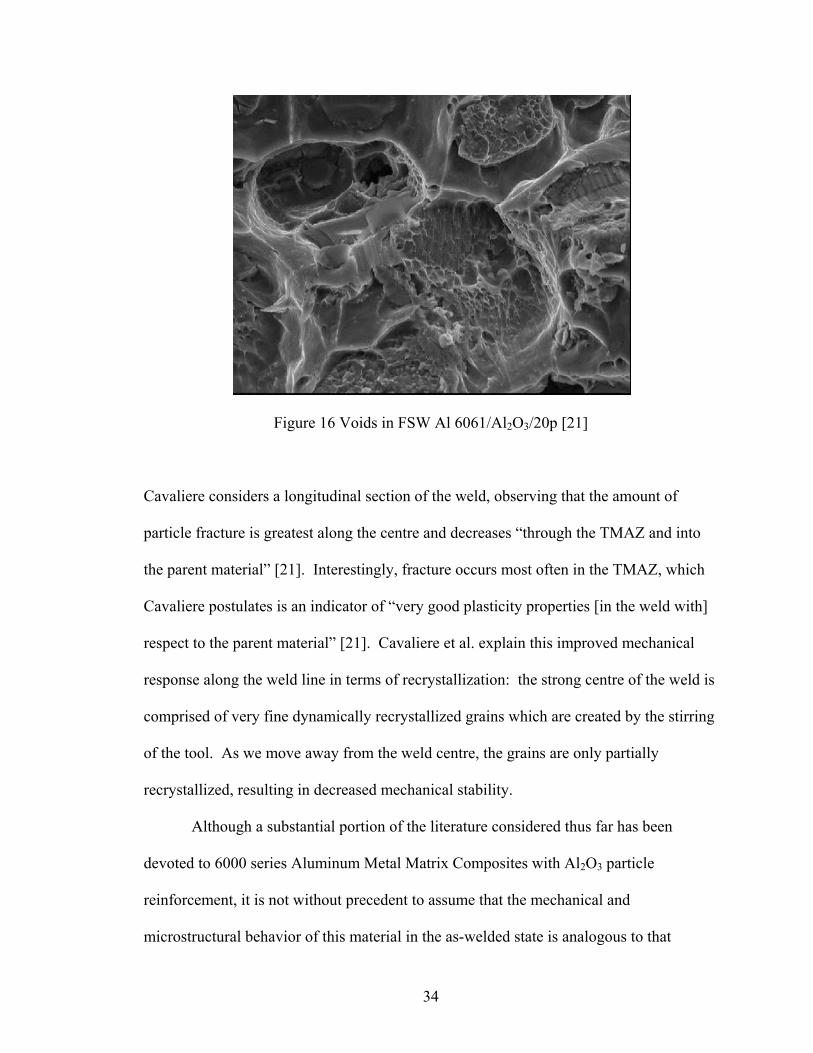
Figure 16 Voids in FSW Al 6061/Al2O3/20p [21]
Cavaliere considers a longitudinal section of the weld, observing that the amount of
particle fracture is greatest along the centre and decreases “through the TMAZ and into
the parent material” [21]. Interestingly, fracture occurs most often in the TMAZ, which
Cavaliere postulates is an indicator of “very good plasticity properties [in the weld with]
respect to the parent material” [21]. Cavaliere et al. explain this improved mechanical
response along the weld line in terms of recrystallization: the strong centre of the weld is
comprised of very fine dynamically recrystallized grains which are created by the stirring
of the tool. As we move away from the weld centre, the grains are only partially
recrystallized, resulting in decreased mechanical stability.
Although a substantial portion of the literature considered thus far has been
devoted to 6000 series Aluminum Metal Matrix Composites with Al2O3 particle
reinforcement, it is not without precedent to assume that the mechanical and
microstructural behavior of this material in the as-welded state is analogous to that
34
exhibited by the composite investigated in our study (Al 6092/SiC/17.5p). In fact, the
overall trends reported in the NASA study of Al 6092/SiC/17.5p are observed for nearly
every variety of Aluminum MMC: severe tool wear, maximum joint efficiencies in the
range of 70-80%, a narrow window of operating parameters, and changes in the pre and
post-weld size and distributions of the reinforcement particles. It should be noted that
although the magnitude of these phenomena may vary with weld parameters, tool
geometry, and/or the type and amount of reinforcement, we can expect to detect them to
some degree in the FSW of any composite material.
We will now consider two studies that are specific to Aluminum MMCs with SiC
particle reinforcement. The first is an article by A.H. Feng et al. entitled “Effect of
microstructural evolution on mechanical properties of AA2009/SiCp composite,” which
examines the effects of FSW on the Silicon Carbide reinforcement particles as well as the
formation of precipitates within the weld nugget [22]. Feng et al. performed butt welds
of ¼” Al 2009/SiC/15p plates using a threaded steel tool with a 1 inch diameter shoulder
and .31 inch diameter probe. Samples were welded at 600 rpm at a travel speed of 2 ipm;
a post weld heat treatment was subsequently used to harden samples to the T4 condition.
Feng et al. used scanning electron microscopy (SEM) to capture images of the material
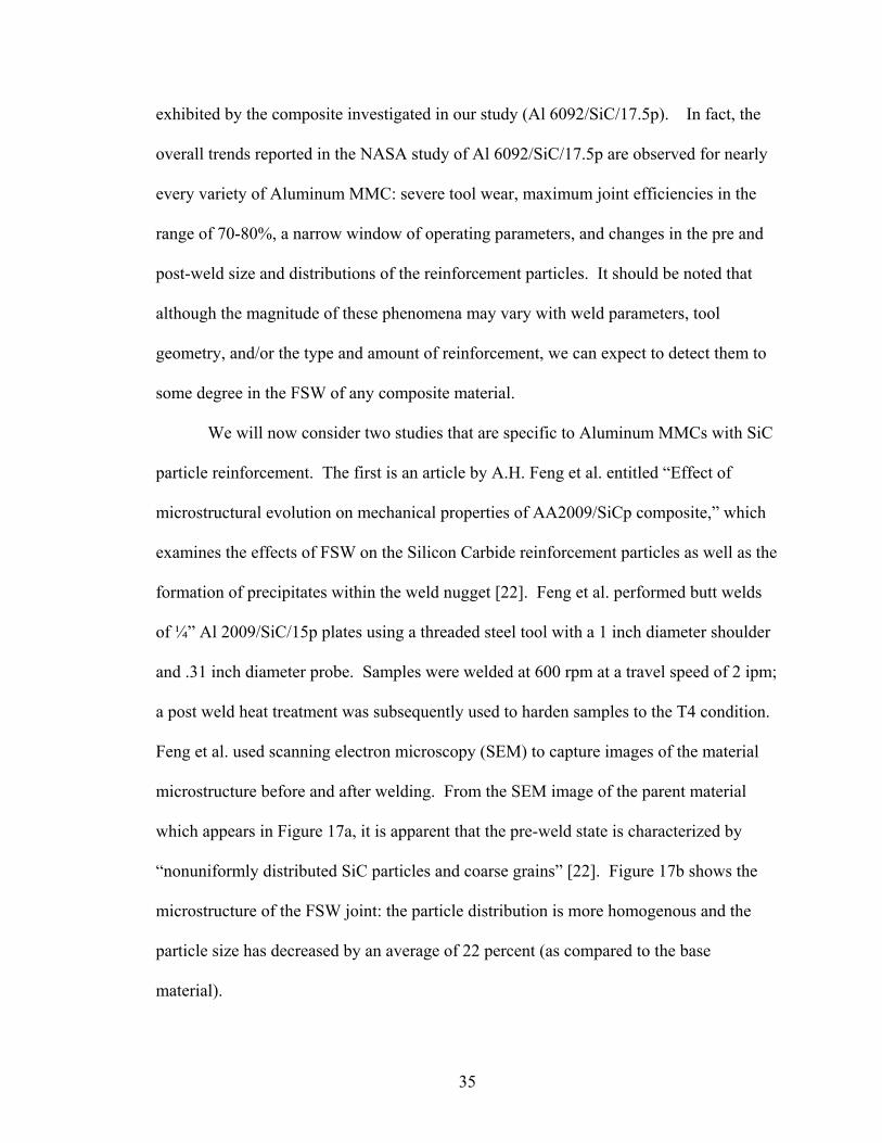
microstructure before and after welding. From the SEM image of the parent material
which appears in Figure 17a, it is apparent that the pre-weld state is characterized by
“nonuniformly distributed SiC particles and coarse grains” [22]. Figure 17b shows the
microstructure of the FSW joint: the particle distribution is more homogenous and the
particle size has decreased by an average of 22 percent (as compared to the base
material).
35
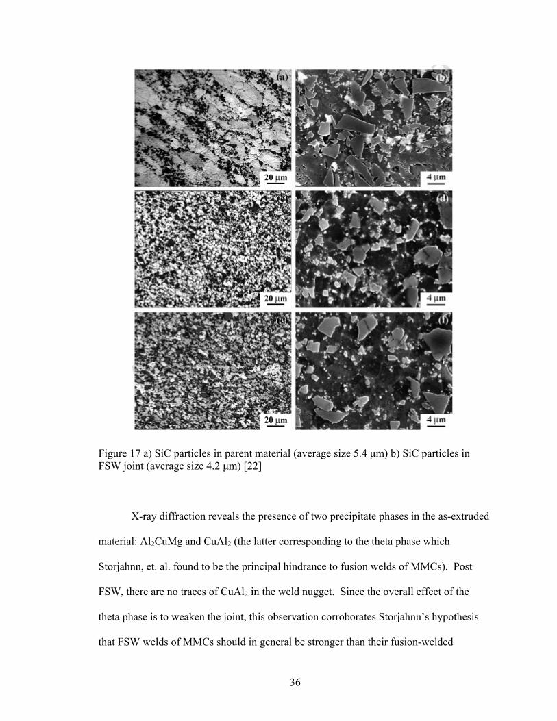
Figure 17 a) SiC particles in parent material (average size 5.4 μm) b) SiC particles in FSW joint (average size 4.2 μm) [22]
X-ray diffraction reveals the presence of two precipitate phases in the as-extruded
material: Al2CuMg and CuAl2 (the latter corresponding to the theta phase which
Storjahnn, et. al. found to be the principal hindrance to fusion welds of MMCs). Post
FSW, there are no traces of CuAl2 in the weld nugget. Since the overall effect of the
theta phase is to weaken the joint, this observation corroborates Storjahnn’s hypothesis
that FSW welds of MMCs should in general be stronger than their fusion-welded
36
counterparts. Feng et al. do detect a θ’’ phase (another form of the CuAl2 precipitate), the
magnitude of which is increased by post-weld heat treatment. However, Feng et al. do
not characterize what effect, if any, this θ’’ phase has on weld integrity or how its
formation varies with weld parameters
The Feng research is significant in that the researchers were able to produce welds
which surpassed the parent material in both yield strength (YS) and ultimate tensile
strength (UTS), a result which had been lacking in previous research. In the best cases
recorded by Feng, the FSW process increases the yield strength of the material by
approximately fifty percent. Interestingly, the as-FSW joint loses some of its strength by
virtue of the heat treatment process. When both the extruded and FSW composite are in
the T4 condition, the YS and UTS of the parent material slightly exceeds that of the
friction stir weld (this strength reduction is attributed to increased formation of the
Cu2FeAl7 phase). These results are shown explicitly in Figure 18, which compares the
UTS, YS, and elongation of Al 2009/SiC/15p pre and post weld.
37
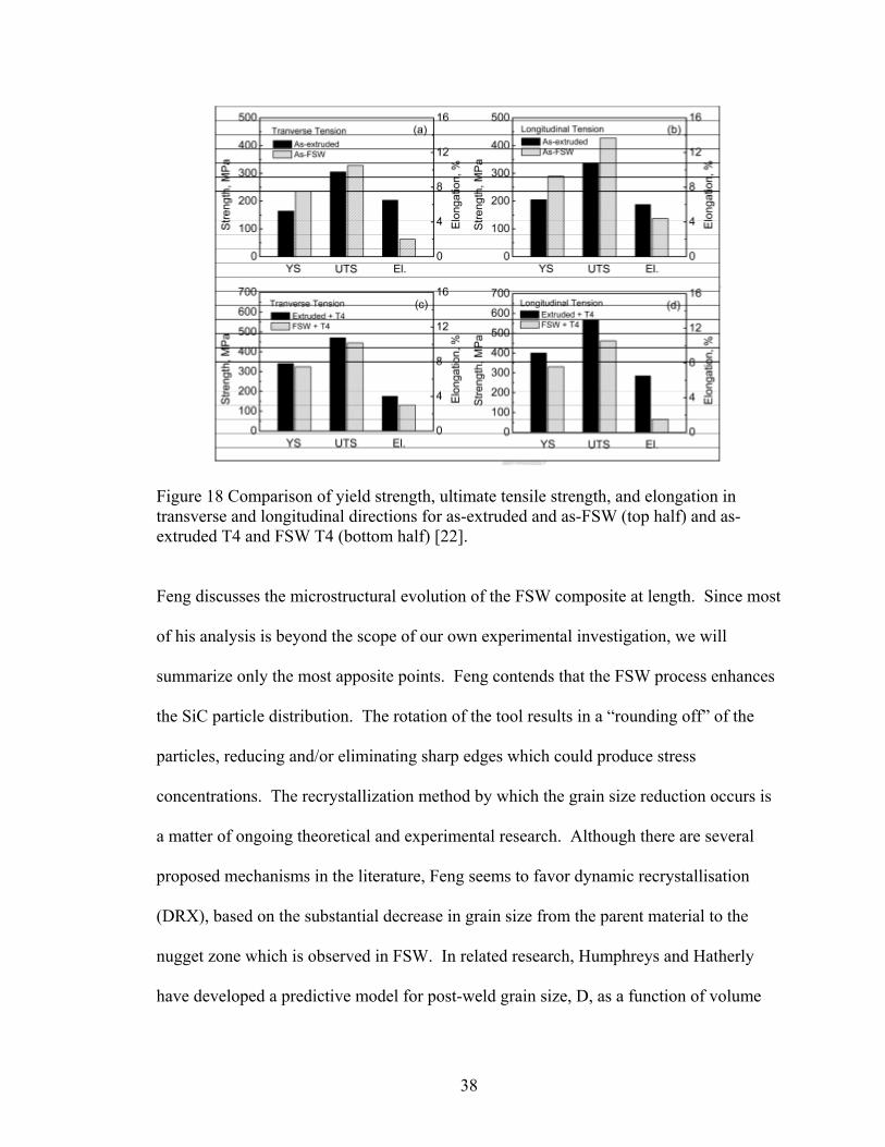
Figure 18 Comparison of yield strength, ultimate tensile strength, and elongation in transverse and longitudinal directions for as-extruded and as-FSW (top half) and as-extruded T4 and FSW T4 (bottom half) [22].
Feng discusses the microstructural evolution of the FSW composite at length. Since most
of his analysis is beyond the scope of our own experimental investigation, we will
summarize only the most apposite points. Feng contends that the FSW process enhances
the SiC particle distribution. The rotation of the tool results in a “rounding off” of the
particles, reducing and/or eliminating sharp edges which could produce stress
concentrations. The recrystallization method by which the grain size reduction occurs is
a matter of ongoing theoretical and experimental research. Although there are several
proposed mechanisms in the literature, Feng seems to favor dynamic recrystallisation
(DRX), based on the substantial decrease in grain size from the parent material to the
nugget zone which is observed in FSW. In related research, Humphreys and Hatherly
have developed a predictive model for post-weld grain size, D, as a function of volume
38
fraction, Fv, and initial particle diameter, d: D = dFv-1/3 [23]. From this simple
relationship, some obvious trends emerge: 1) the resultant FSW grain size is directly
proportional to the grain size of the parent material and 2) the post weld grain size
decreases with increasing volume fraction. When Feng et al. apply the
Humphrey/Hatherly model to their research on 2009/SiC/15p, they find that it over-
predicts the FSW grain size by approximately sixty percent. Feng ascribes this to the
model’s failure to account for the formation of precipitate and diffusion phenomena.
Klug, et. al. have proposed an experimentally-based model to estimate the amount of
Cu2FeAl7 formed in composites [24]. The Klug equation relates the intensity of fraction
lines in XRD analysis to phase weight fractions (which can be obtained through mass
spectroscopy). The limitation of the Klug model lies in its dependence on tool wear, a
variable that is paramount to joining of MMCs yet is noticeably absent from the Klug
formulation. Feng suggests that the Klug equation is most appropriate is best suited for
scenarios in which tool wear is minimized by the use of “wear-resistant tool materials” or
abrasive coatings [22].
A characterization of tool wear in an Aluminum material reinforced by SiC was
completed by G.J. Fernandez and L.E. Murr of the University of Texas at El Paso.
Fernandez and Murr performed butt welds of MMCs using a threaded probe of diameter
0.25” and measuring 0.147” in length (the probe length is smaller than usual to
correspond to the reduced plate thickness of 0.157”). Rotation speeds considered in the
study were 500, 750, and 1000 RPM; travel speeds were fixed at 25.8 and 14.2 IPM.
Tool wear of the probe was measured using an optical technique in which the post-weld
probe shapes in magnified photographs were cut out and compared with the original
39
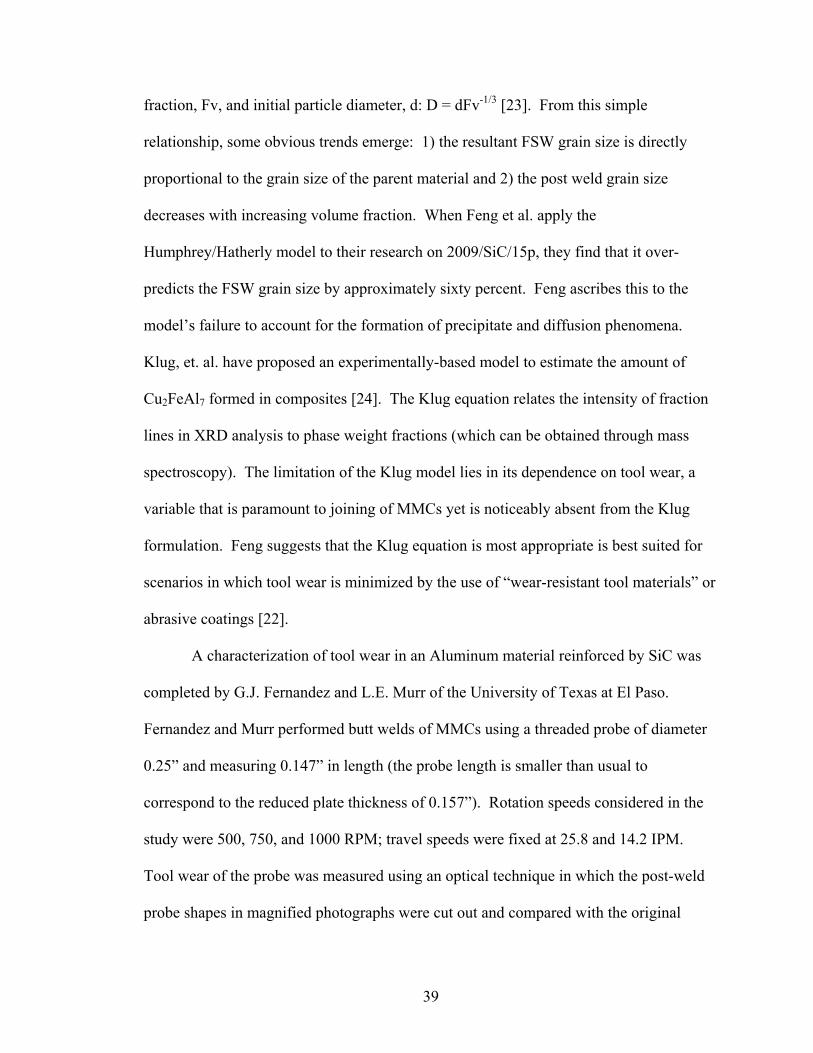
probe shape [25]. Tool wear could then be expressed quantitatively in terms of volume
consumption. Figure 19 shows the plot of probe wear as a function of travel distance for
rotation speeds of 500, 750, and 1000. It is clear that wear is most dramatic at 1000
RPM, a result which corroborates the results of an earlier study by Prado et al. on Al
6061/Al2O3/20p [26].
Figure 19 Wear versus traverse distance for 500, 750, and 1000 RPM. Travel speed was held constant at 14.2 IPM [25].
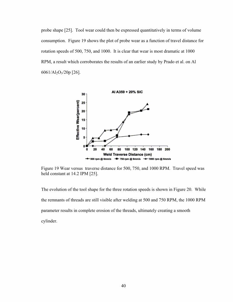
The evolution of the tool shape for the three rotation speeds is shown in Figure 20. While
the remnants of threads are still visible after welding at 500 and 750 RPM, the 1000 RPM
parameter results in complete erosion of the threads, ultimately creating a smooth
cylinder.
40
Figure 20 Sequence of probe wear for a) 500 RPM, b) 750 RPM, and c) 1000 RPM as a function of travel distance in meters [25].
The complete plot of probe wear for the range of parameters considered is shown in
Figure 21. From the graph, Feng discerns that the parameters which minimize wear are a
rotation speed of 500 rpm and a travel speed of 24 in/min. At these conditions, wear is
less than 10% (as compared to 30% for the worst case of 1000 RPM and 2.4 IPM).
41
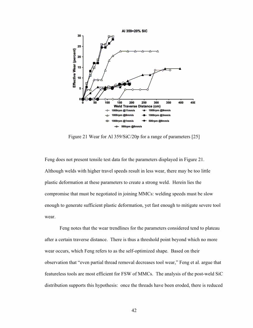
Figure 21 Wear for Al 359/SiC/20p for a range of parameters [25]
Feng does not present tensile test data for the parameters displayed in Figure 21.
Although welds with higher travel speeds result in less wear, there may be too little
plastic deformation at these parameters to create a strong weld. Herein lies the
compromise that must be negotiated in joining MMCs: welding speeds must be slow
enough to generate sufficient plastic deformation, yet fast enough to mitigate severe tool
wear.
Feng notes that the wear trendlines for the parameters considered tend to plateau
after a certain traverse distance. There is thus a threshold point beyond which no more
wear occurs, which Feng refers to as the self-optimized shape. Based on their
observation that “even partial thread removal decreases tool wear,” Feng et al. argue that
featureless tools are most efficient for FSW of MMCs. The analysis of the post-weld SiC
distribution supports this hypothesis: once the threads have been eroded, there is reduced
42
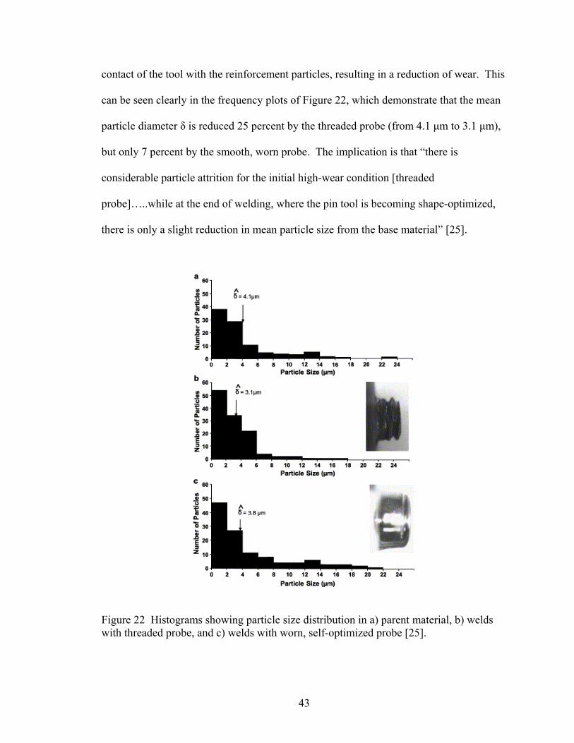
contact of the tool with the reinforcement particles, resulting in a reduction of wear. This
can be seen clearly in the frequency plots of Figure 22, which demonstrate that the mean
particle diameter δ is reduced 25 percent by the threaded probe (from 4.1 μm to 3.1 μm),
but only 7 percent by the smooth, worn probe. The implication is that “there is
considerable particle attrition for the initial high-wear condition [threaded
probe]…..while at the end of welding, where the pin tool is becoming shape-optimized,
there is only a slight reduction in mean particle size from the base material” [25].
Figure 22 Histograms showing particle size distribution in a) parent material, b) welds with threaded probe, and c) welds with worn, self-optimized probe [25].
43
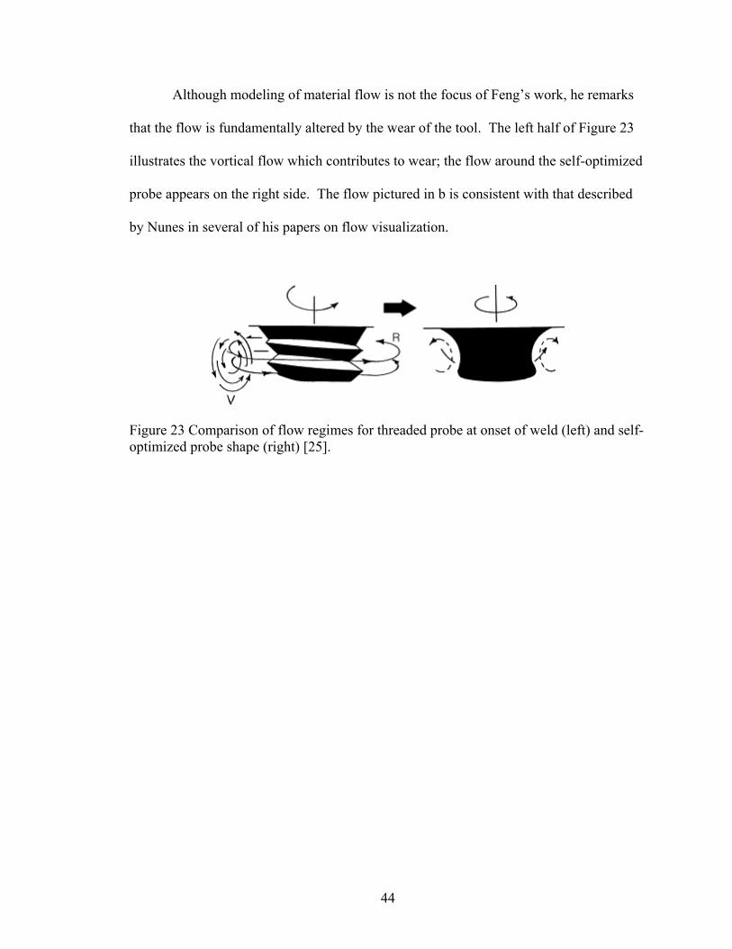
Although modeling of material flow is not the focus of Feng’s work, he remarks
that the flow is fundamentally altered by the wear of the tool. The left half of Figure 23
illustrates the vortical flow which contributes to wear; the flow around the self-optimized
probe appears on the right side. The flow pictured in b is consistent with that described
by Nunes in several of his papers on flow visualization.
Figure 23 Comparison of flow regimes for threaded probe at onset of weld (left) and self-optimized probe shape (right) [25].
44
CHAPTER III
EXPERIMENTAL PROCEDURE
We will now detail the experimental conditions under which the research
presented in subsequent chapters was conducted. The overall goal of the experimentation
was to establish an optimized working envelope for the welding of Al 6061 and Al
6061/SiC/17.5p using coated and uncoated tools. The force and torque data was also
analyzed to determine the effect of the coating on the loads experienced by the tool
during the weld cycle. This chapter outlines the experimental configuration of the
Vanderbilt University Welding Automation Laboratory apparatus for Friction Stir
Welding, post-weld mechanical testing and microscopy procedures, the use of optical
comparators to assess tool wear, and the processing of data.
3.1 Overview of the FSW Apparatus
The Vanderbilt University Welding Automation Laboratory uses a Milwaukee
#2K Universal Milling Machine modified for Friction Stir Welding. A photo of the
entire apparatus with the components labeled appears in Figure 24. The Heavy Duty
Kearney and Trecker Vertical Head Attachment functions as a fastening mechanism
which prevents movement along the vertical axis of the mill. Additionally, a Baldor
Industrial VM 2514, 20 Horsepower, 3Phase 230 VAC motor rated for rotation speeds of
3450 RPM is affixed to the vertical head, driving the spindle by means of a belt and
pulley system. The larger driven pulley (Emerson/Browning/Morse 16J60P) measures 6
45
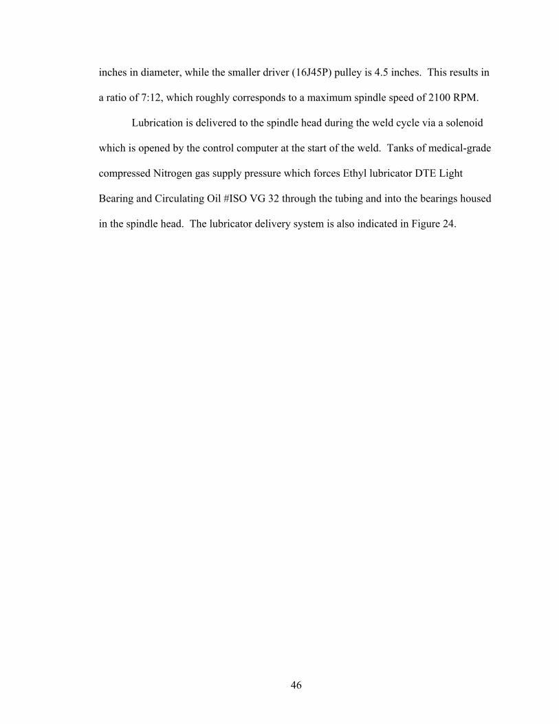
inches in diameter, while the smaller driver (16J45P) pulley is 4.5 inches. This results in
a ratio of 7:12, which roughly corresponds to a maximum spindle speed of 2100 RPM.
Lubrication is delivered to the spindle head during the weld cycle via a solenoid
which is opened by the control computer at the start of the weld. Tanks of medical-grade
compressed Nitrogen gas supply pressure which forces Ethyl lubricator DTE Light
Bearing and Circulating Oil #ISO VG 32 through the tubing and into the bearings housed
in the spindle head. The lubricator delivery system is also indicated in Figure 24.
46
Lateral motor
Lubricator delivery system
Vertical head
20 HP motor
Kistler Dynamometer
Locking set screw
Vertical motor
Transverse motor
Backing plate and clamping system
V-Belt and Pulley System
Figure 24 Overview of FSW apparatus
47
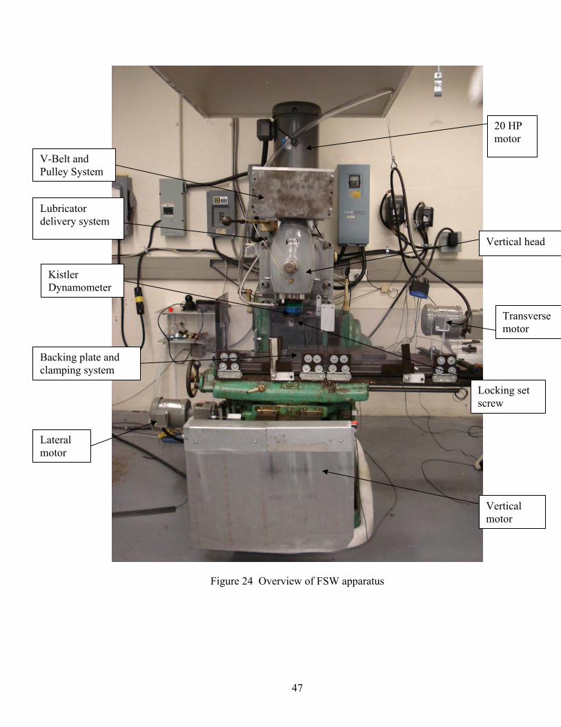
The blue-green instrument which is visible directly below the vertical head is the
Kistler Rotating Cutting Force Dynamometer, which is responsible for in-process
recordings of forces in the x, y, and z directions as well as torque. The base of the
dynamometer is outfitted with two optical encoders. The lower interrupter functions to
decouple the forces in the longitudinal and transverse directions, while the uppermost
interrupter is responsible for counting the number of revolutions. The spacing between
the teeth of the axis interrupter is 36 degrees. A close-up of the dynamometer and optical
encoders appears in Figure 25. The laser transmitter works in tandem with the optical
interrupters and transmits a signal through the NI-DAQ each time the light transitions
from blocked to un-blocked.
Figure 25 Dynamometer and optical encoders
Axis reference interrupter
Revolution interrupter
Laser transmitter
The locking set screw by which the FSW tool is inserted into the machine is located
directly beneath the dynamometer. The tool is positioned with the probe to be used in
48
welding facing downward toward the backing plate. A square indentation (½ x ½” x
1/10”) which has been milled into the upper portion of the tool is aligned with the double
set screw. Once proper alignment is achieved, both set screws are securely tightened
using an Allen wrench, thus ensuring that the tool will not deflect or oscillate vertically
during the course of the weld.
The weld sample rests on top of a backing plate composed of cold-rolled steel
with dimensions of 24” x 7” x 1.” The sample is clamped into place using a clamping
scheme which consists of twenty bolt holes (ten on each side of the sample) which are
tightened to 50 N-m using a torque wrench. The purpose of the clamping is to prevent the
movement of the sample during the weld process; insufficient clamping can result in
bowing or gapping of the material. Though the samples used in this research are only 9”x
3”, the clamping and backing plate are large enough to accommodate samples which
measure 30” x 5”. In the case of bead on plate welds, the sample dimensions for this
research are 9”x 3”x ¼”. For butt welds, the sample consists of two pieces, each
measuring 9” x 1 ½ ” x ¼” thick which are aligned so that the FSW tool can traverse a
straight line between them to produce a joint.
3.2 Lateral, Traverse, Vertical Motors and Position Control
The positioning and travel of the tool is controlled by the three external motor
drives which are used to move the table in the x, y, and z directions. The lateral and
traverse motors are both U.S. Electronic 1 Horsepower motors of type TF GDY TE. The
lateral motor, which moves the stage in or out in a direction perpendicular to the weld
path, has a gear ratio of 6.02 and a minimum speed of 1.7 inches per minute. The lateral
49
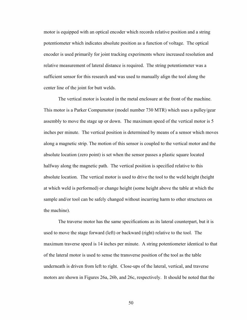
motor is equipped with an optical encoder which records relative position and a string
potentiometer which indicates absolute position as a function of voltage. The optical
encoder is used primarily for joint tracking experiments where increased resolution and
relative measurement of lateral distance is required. The string potentiometer was a
sufficient sensor for this research and was used to manually align the tool along the
center line of the joint for butt welds.
The vertical motor is located in the metal enclosure at the front of the machine.
This motor is a Parker Compumotor (model number 730 MTR) which uses a pulley/gear
assembly to move the stage up or down. The maximum speed of the vertical motor is 5
inches per minute. The vertical position is determined by means of a sensor which moves
along a magnetic strip. The motion of this sensor is coupled to the vertical motor and the
absolute location (zero point) is set when the sensor passes a plastic square located
halfway along the magnetic path. The vertical position is specified relative to this
absolute location. The vertical motor is used to drive the tool to the weld height (height
at which weld is performed) or change height (some height above the table at which the
sample and/or tool can be safely changed without incurring harm to other structures on
the machine).
The traverse motor has the same specifications as its lateral counterpart, but it is
used to move the stage forward (left) or backward (right) relative to the tool. The
maximum traverse speed is 14 inches per minute. A string potentiometer identical to that
of the lateral motor is used to sense the transverse position of the tool as the table
underneath is driven from left to right. Close-ups of the lateral, vertical, and traverse
motors are shown in Figures 26a, 26b, and 26c, respectively. It should be noted that the
50
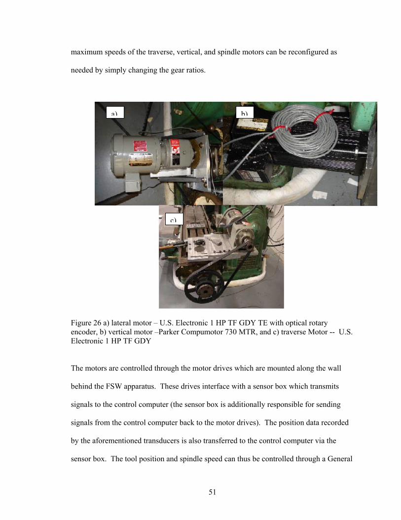
maximum speeds of the traverse, vertical, and spindle motors can be reconfigured as
needed by simply changing the gear ratios.
a) b)
c)
Figure 26 a) lateral motor – U.S. Electronic 1 HP TF GDY TE with optical rotary encoder, b) vertical motor –Parker Compumotor 730 MTR, and c) traverse Motor -- U.S. Electronic 1 HP TF GDY
The motors are controlled through the motor drives which are mounted along the wall
behind the FSW apparatus. These drives interface with a sensor box which transmits
signals to the control computer (the sensor box is additionally responsible for sending
signals from the control computer back to the motor drives). The position data recorded
by the aforementioned transducers is also transferred to the control computer via the
sensor box. The tool position and spindle speed can thus be controlled through a General
51
User Interface known as “Weld Controller” on the control computer. “Weld Controller,”
written in Dynamic C by graduate student Paul Fleming, effectively automates the entire
weld cycle. A screenshot of the control program in use appears in Figure 27.
Figure 27 Screenshot of “Weld Controller”
The procedure for performing a typical weld operation using “Weld Controller” is
outlined below:
1. Once the tool and sample to be welded are in place, the sensor box, motor drives,
and dynamometer are turned on and connected to through the GUI.
2. The vertical motor is zeroed by raising or lowering the stage until the magnetic
strip encoder has passed the reference mark.
52

3. Weld parameters are entered by the user. These include the start and end
locations for the weld, plunge depth, spindle speed, traverse rate, return height,
change height and the Autozero location.
4. The Autozero location should roughly coincide with the “end” of the sample. The
Autozero function in “Weld Controller” will lower the tool until the shoulder
contacts the material. Manual adjustments are made as necessary to ensure that
the shoulder (rather than the probe) contacts the edge of the sample.
5. The pressure is turned on and the lubricator is activated by clicking the
appropriate button in the control program. When lubricant can be seen flowing
freely through the tubes which deliver lubricant to the spindle, the lubricator is
turned off and the weld can commence. It is only necessary to run the lubricator
in this manner for the first weld in a series; once the user clicks “Weld”, the
lubricator is started automatically.
6. Click “Weld” to initiate the weld. Note that the tool must already be in the start
position; this can be easily achieved by clicking “go home.” The spindle will start
and the tool will gradually “creep” into the material: the creep period ensures that
there is sufficient plastic deformation for welding, thus helping to prevent tool
fracture. After a few seconds of creep, the machine will weld the sample at the
parameters specified by the user. When the tool reaches the end location, the
spindle will stop and the tool will return to the change height. The welded sample
can then be exchanged with new material and the weld process can be repeated.
53
During the course of a weld, force and torque recordings are made by the Kistler
dynamometer. These files are stored on a second computer separate from that which
controls the weld. After the weld is complete, its corresponding data file can be accessed
and exported to Microsoft Excel for post-processing and analysis.
3.3 Post-weld analysis: Metallography
In order to assess the quality of a weld using microscopy techniques, the material
must first be prepared through a sequence of cutting, polishing and etching to reveal the
microstructure of the finished joint. Initially a 1”x 3”x ¼ ” piece of the sample is cut
away using a band saw. This piece is usually taken from the middle of the sample to
ensure that the cross-section will be representative of the steady state process (i.e. free of
the anomalous microstructure which may accompany the entrance or exit of the tool from
the material). A second cut is then made along the longitudinal axis of this smaller piece
of weld using a diamond saw. After cutting is complete, the weld cross-section should
measure no more than ¼” x ½” x ¼”. The cross-section is then mounted using a
thermosetting epoxy molding compound. The mold compound encapsulates the cross-
section and, when placed in an environment of sufficient heat and pressure, cures around
it. The ultimate result is a black cylinder approximately 1” in diameter and ¾” in height
with the weld cross-section exposed on one of the circular faces. The edges of the
cylinder are chamfered to augment the polishing process. The cross-section is then
polished on a polishing wheel using successively finer grades of Silicon Carbide paper.
The grades range from the coarsest at 300 grit to the finest at 3600 grit, with
intermediates of 600, 800, 1200, 1600, and 2400. At the end of the polishing stage, the
54
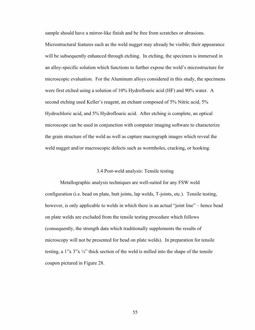
sample should have a mirror-like finish and be free from scratches or abrasions.
Microstructural features such as the weld nugget may already be visible; their appearance
will be subsequently enhanced through etching. In etching, the specimen is immersed in
an alloy-specific solution which functions to further expose the weld’s microstructure for
microscopic evaluation. For the Aluminum alloys considered in this study, the specimens
were first etched using a solution of 10% Hydroflouric acid (HF) and 90% water. A
second etching used Keller’s reagent, an etchant composed of 5% Nitric acid, 5%
Hydrochloric acid, and 5% Hydroflouric acid. After etching is complete, an optical
microscope can be used in conjunction with computer imaging software to characterize
the grain structure of the weld as well as capture macrograph images which reveal the
weld nugget and/or macroscopic defects such as wormholes, cracking, or hooking.
3.4 Post-weld analysis: Tensile testing
Metallographic analysis techniques are well-suited for any FSW weld
configuration (i.e. bead on plate, butt joints, lap welds, T-joints, etc.). Tensile testing,
however, is only applicable to welds in which there is an actual “joint line” – hence bead
on plate welds are excluded from the tensile testing procedure which follows
(consequently, the strength data which traditionally supplements the results of
microscopy will not be presented for bead on plate welds). In preparation for tensile
testing, a 1”x 3”x ¼” thick section of the weld is milled into the shape of the tensile
coupon pictured in Figure 28.
55
Figure 28 Sketch of coupon used in tensile testing.
These tensile coupons, which are designed in accordance with ASTM standards for
mechanical testing, are assessed using an MTS machine equipped with a hydraulic press
for tensile and compression testing. The thickness and width of the specimen are
measured by the user and input into the computer prior to testing. As the coupon is pulled
apart, the computer records the stress, strain, ultimate tensile strength (UTS), yield
strength (YS), and percent elongation. This data file can then be used to generate plots of
stress versus strain and/or load versus extension. Results of tensile tests are usually
specified in terms of joint efficiency, defined as the ratio of the UTS of the weld
specimen to the UTS of the parent material expressed as a percentage. Ideally, a tensile
specimen will have a joint efficiency of greater than 70% and break outside the weld line.
A “good” weld is characterized by both high joint efficiency and a defect-free
macrosection, criteria which will be discussed further in the chapters on experimental
results.
56
3.5 Shadowgraph
A shadowgraph technique was used as an optical comparator to measure tool wear
in welds of Metal Matrix Composites (MMCs). The shadowgraph machine works largely
in the same manner as an overhead projector, using a Fresnel lens to focus the light from
a lamp aimed at the specimen. Each wear study begins with an unused FSW tool which
serves as a baseline. The shadowgraph of the unworn tool is then compared with
successive shadowgraphs of the tool post-weld. In this manner, the shadowgraph is used
to provide a visual representation of tool wear which supplements the quantitative data.
Specifics of the shadowgraph technique and how they were applied to this research will
be further discussed in Chapter V.
57
CHAPTER IV
EXPERIMENTAL RESULTS FOR SMOOTH PROBE FSW TOOLS ON AL 6061
Experimental results for welds performed on Aluminum 6061 using an uncoated steel
tool and a Molybdenum tool of identical geometry coated with diamond by Chemical
Vapor Deposition will be compared in this chapter. The primary basis for comparison is
the measurement of longitudinal force, transverse force, axial force, and torque recorded
during welding by the dynamometer. The principal limitation in robotic applications of
Friction Stir Welding is axial force. Thus, any reduction in axial force which is attained
through the use of a coated tool is advantageous from a robotics standpoint. To ascertain
that this decrease in axial force is not accompanied by a decline in weld quality,
macrosections of welds performed at identical parameters using the uncoated and coated
tool were also evaluated.
4.1 Tool Design
The tool geometry considered in this stage of the research was a smooth
cylindrical probe. Although the tool was devoid of the features (threads, flats, flutes, etc.)
which enhance vertical stirring and often result in a better quality weld, the smooth probe
was chosen for its simple geometry and ease of machining. Additionally, the welds
performed on Al 6061 were all “bead on plate” welds; the emphasis was on comparative
analysis of force data rather than optimization of weld quality. The tool dimensions were
based on the previous research of graduate student Reginald Crawford [27]. All tools in
58
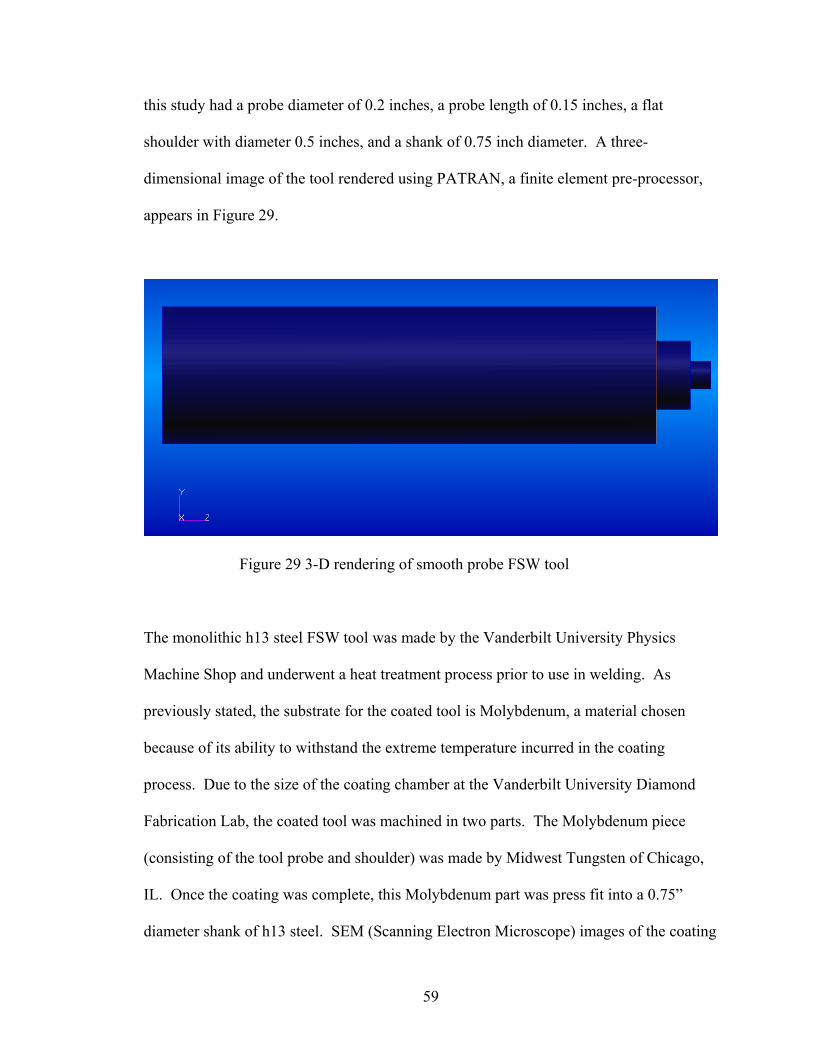
this study had a probe diameter of 0.2 inches, a probe length of 0.15 inches, a flat
shoulder with diameter 0.5 inches, and a shank of 0.75 inch diameter. A three-
dimensional image of the tool rendered using PATRAN, a finite element pre-processor,
appears in Figure 29.
Figure 29 3-D rendering of smooth probe FSW tool
The monolithic h13 steel FSW tool was made by the Vanderbilt University Physics
Machine Shop and underwent a heat treatment process prior to use in welding. As
previously stated, the substrate for the coated tool is Molybdenum, a material chosen
because of its ability to withstand the extreme temperature incurred in the coating
process. Due to the size of the coating chamber at the Vanderbilt University Diamond
Fabrication Lab, the coated tool was machined in two parts. The Molybdenum piece
(consisting of the tool probe and shoulder) was made by Midwest Tungsten of Chicago,
IL. Once the coating was complete, this Molybdenum part was press fit into a 0.75”
diameter shank of h13 steel. SEM (Scanning Electron Microscope) images of the coating
59
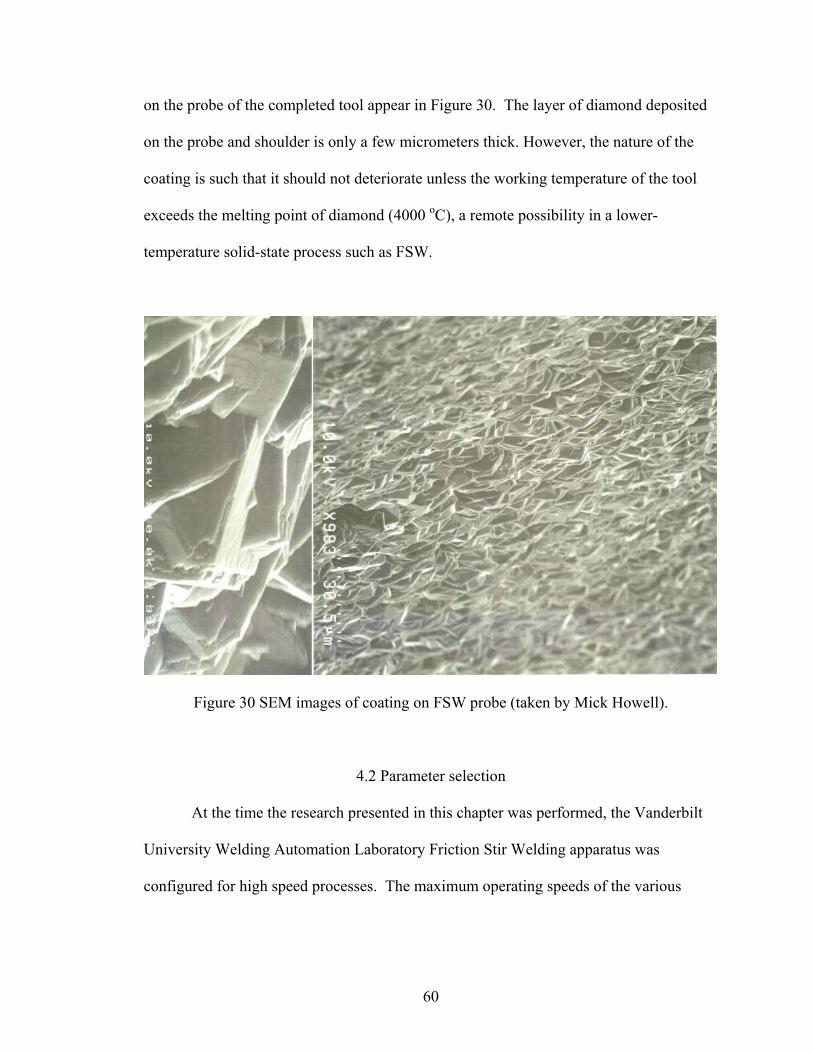
on the probe of the completed tool appear in Figure 30. The layer of diamond deposited
on the probe and shoulder is only a few micrometers thick. However, the nature of the
coating is such that it should not deteriorate unless the working temperature of the tool
exceeds the melting point of diamond (4000 oC), a remote possibility in a lower-
temperature solid-state process such as FSW.
Figure 30 SEM images of coating on FSW probe (taken by Mick Howell).
4.2 Parameter selection
At the time the research presented in this chapter was performed, the Vanderbilt
University Welding Automation Laboratory Friction Stir Welding apparatus was
configured for high speed processes. The maximum operating speeds of the various
60
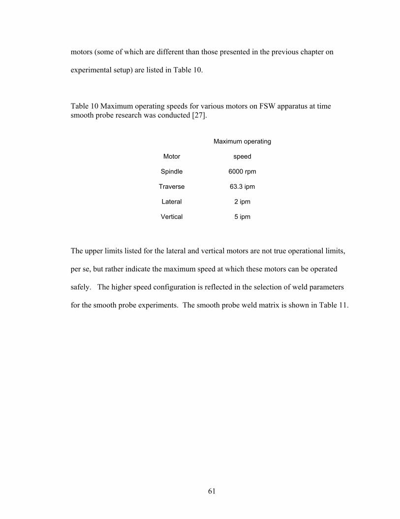
motors (some of which are different than those presented in the previous chapter on
experimental setup) are listed in Table 10.
Table 10 Maximum operating speeds for various motors on FSW apparatus at time smooth probe research was conducted [27].
Motor
Maximum operating
speed
Spindle 6000 rpm
Traverse 63.3 ipm
Lateral 2 ipm
Vertical 5 ipm
The upper limits listed for the lateral and vertical motors are not true operational limits,
per se, but rather indicate the maximum speed at which these motors can be operated
safely. The higher speed configuration is reflected in the selection of weld parameters
for the smooth probe experiments. The smooth probe weld matrix is shown in Table 11.
61
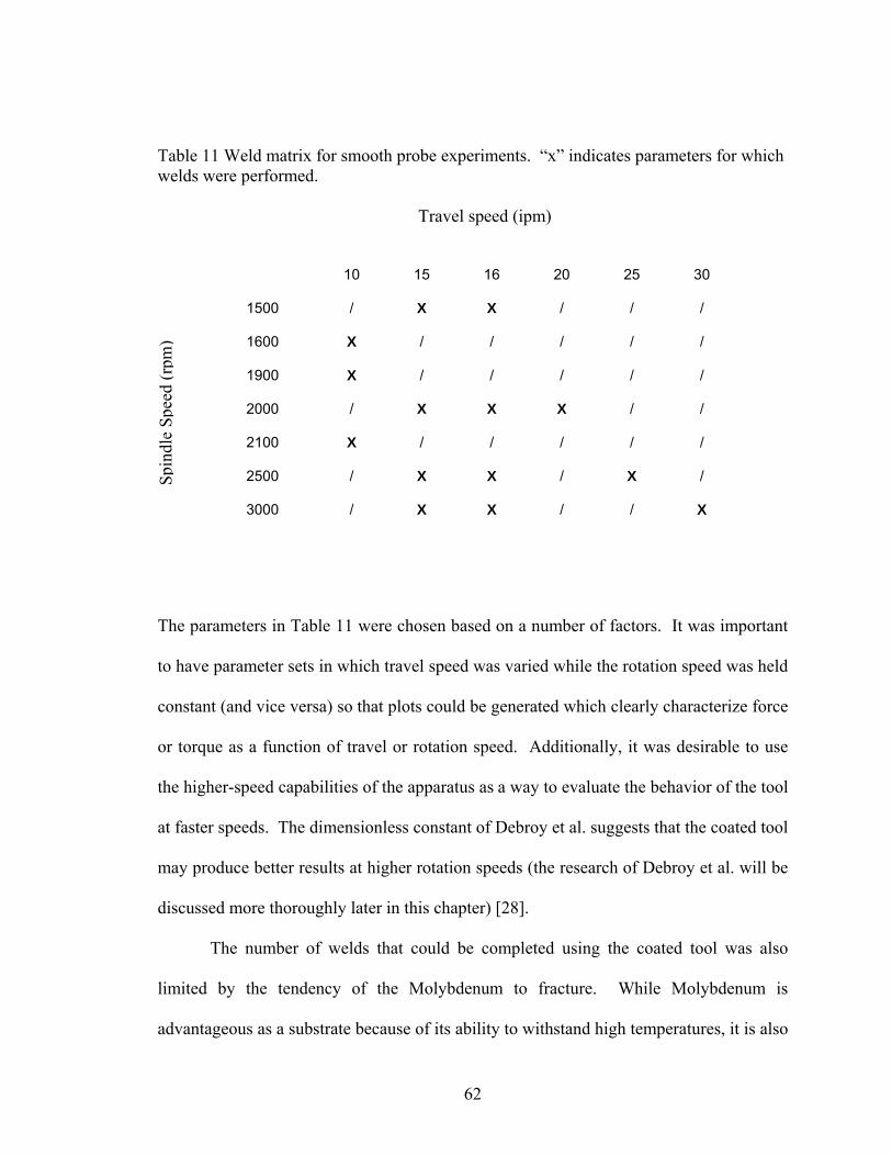
Table 11 Weld matrix for smooth probe experiments. “x” indicates parameters for which welds were performed.
Travel speed (ipm)
10 15 16 20 25 30
1500 / X X / / /
1600 X / / / / /
1900 X / / / / /
2000 / X X X / /
2100 X / / / / /
2500 / X X / X /
3000 / X X / / X
Spin
dle
Spee
d (r
pm)
The parameters in Table 11 were chosen based on a number of factors. It was important
to have parameter sets in which travel speed was varied while the rotation speed was held
constant (and vice versa) so that plots could be generated which clearly characterize force
or torque as a function of travel or rotation speed. Additionally, it was desirable to use
the higher-speed capabilities of the apparatus as a way to evaluate the behavior of the tool
at faster speeds. The dimensionless constant of Debroy et al. suggests that the coated tool
may produce better results at higher rotation speeds (the research of Debroy et al. will be
discussed more thoroughly later in this chapter) [28].
The number of welds that could be completed using the coated tool was also
limited by the tendency of the Molybdenum to fracture. While Molybdenum is
advantageous as a substrate because of its ability to withstand high temperatures, it is also
62
very brittle and prone to fracture when it undergoes stress. Of the three original coated
tools set aside for this portion of the research, two of the three failed. Specifically, the
probe sheared off upon entrance into the workpiece material. This shearing phenomenon
is even more pronounced in uncoated Molybdenum (the coated Molybdenum tool may be
less brittle because it has been subjected to the high temperature environment of the
coating chamber, a process analogous to heat treatment). It may be possible to reduce the
incidence of probe failure by pre-drilling a hole with a diameter slightly larger than that
of the probe into the workpiece material. This would enable the shoulder of the tool to
fully contact the material before the probe, creating a preheat zone which would
plasticize the material and reduce stresses on the probe as it enters the material. The
effect of pre-drilling will be assessed more fully in a subsequent chapter.
For all welds, the tool tilt angle was fixed at 20 and the plunge depth was set at
0.004 inches. The latter specification indicates that the tool plunges an additional 0.004
inches below the zero point before welding begins (this is done to ensure sufficient
shoulder contact with the workpiece material). A 0.15 inch probe length, 0.25 inch thick
material, and a plunge depth of 0.004 inches result in a weld ligament (distance from the
probe tip to the backing plate) of 0.096 inches. This is a rather large ligament (for butt
welds the optimal value can be as small as 0.01 inches), but it is acceptable for the
research presented in this chapter. Since we are performing bead on plate welds and are
primarily concerned with the recording of force data rather than the ultimate strength of
the weld (these welds were not subjected to tensile tests), a partial penetration weld is
sufficient.
63
4.3 Results: General trends in force data for the uncoated steel smooth probe FSW tool
Several welds were performed for each parameter set in the weld matrix of Figure 11.
In most cases, at least two welds with the same tool were performed at a given parameter.
If there were any anomalies in the force data for a tool/parameter combination (typically
a variation of more than ten percent), a third weld was completed.
Values for force and torque (Fx, Fy, Fz, and Mz) are extracted from an Excel
spreadsheet which compiles the data recorded by the dynamometer. The dynamometer
records ten samples per revolution – hence a typical weld file can contain anywhere from
25,000 to upwards of 60,000 data points, depending on the length of the weld. A
significant segment of this data is recorded either in the period before the actual weld
commences or after the tool has exited the material. Hence the best way to obtain a
steady state value for force is to graph the dynamometer data versus time in Excel and
then visually estimate the cells which contain steady state data. This method is not as
imprecise as it may initially seem. Figure 31 shows a typical force vs. time graph for a
steel tool welding Aluminum 6061 at 2000 rpm and 20 ipm. The flat lines on the left and
right sides of the graph correspond to the period before and after the tool engages with
the material, respectively. The high plateau in the center of the graph corresponds to the
steady-state weld condition, while the lower plateau coincides with the “creep” (the phase
in which the tool dwells in the material to generate sufficient heat for welding).
64
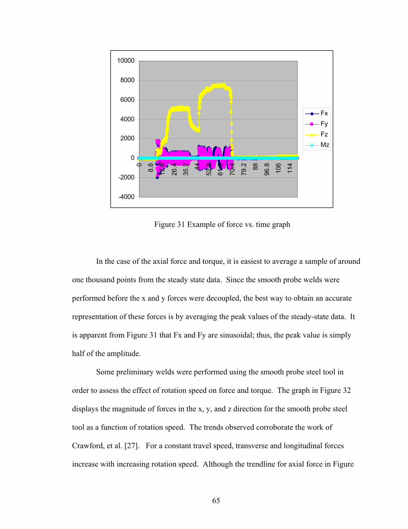
-4000
-2000
0
2000
4000
6000
8000
10000
0
8.8
17.6
26.4
35.2 44
52.8
61.6
70.4
79.2 88
96.8
106
114
FxFyFzMz
Figure 31 Example of force vs. time graph
In the case of the axial force and torque, it is easiest to average a sample of around
one thousand points from the steady state data. Since the smooth probe welds were
performed before the x and y forces were decoupled, the best way to obtain an accurate
representation of these forces is by averaging the peak values of the steady-state data. It
is apparent from Figure 31 that Fx and Fy are sinusoidal; thus, the peak value is simply
half of the amplitude.
Some preliminary welds were performed using the smooth probe steel tool in
order to assess the effect of rotation speed on force and torque. The graph in Figure 32
displays the magnitude of forces in the x, y, and z direction for the smooth probe steel
tool as a function of rotation speed. The trends observed corroborate the work of
Crawford, et al. [27]. For a constant travel speed, transverse and longitudinal forces
increase with increasing rotation speed. Although the trendline for axial force in Figure
65
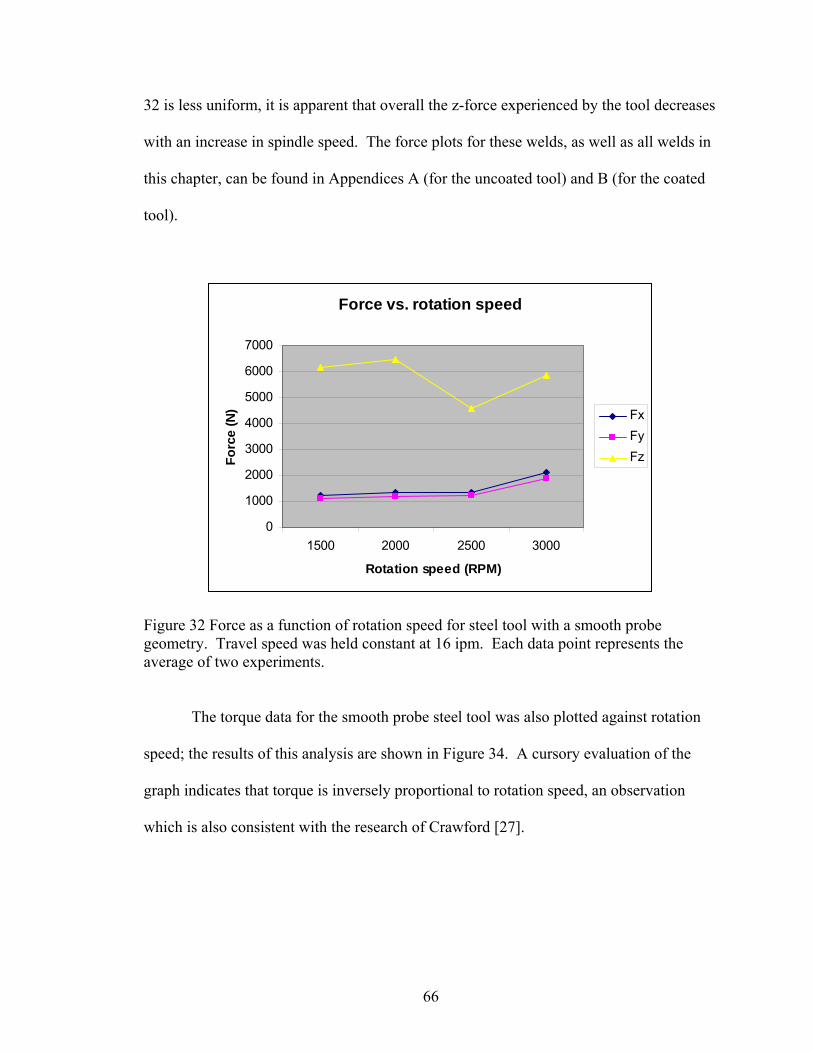
32 is less uniform, it is apparent that overall the z-force experienced by the tool decreases
with an increase in spindle speed. The force plots for these welds, as well as all welds in
this chapter, can be found in Appendices A (for the uncoated tool) and B (for the coated
tool).
Force vs. rotation speed
0
1000
2000
3000
4000
5000
6000
7000
1500 2000 2500 3000
Rotation speed (RPM)
Forc
e (N
) FxFyFz
Figure 32 Force as a function of rotation speed for steel tool with a smooth probe geometry. Travel speed was held constant at 16 ipm. Each data point represents the average of two experiments.
The torque data for the smooth probe steel tool was also plotted against rotation
speed; the results of this analysis are shown in Figure 34. A cursory evaluation of the
graph indicates that torque is inversely proportional to rotation speed, an observation
which is also consistent with the research of Crawford [27].
66

Torque vs. Rotation speed
02468
101214161820
1500 2000 2500 3000
Rotation speed (RPM)
Torq
ue (N
-m)
Mz
Figure 33 Plot of torque vs. rotation speed for steel tool with smooth probe geometry. Travel rate is constant at 16 ipm.
The formulation for power in FSW is 2π x torque x RPM/60. The units of power in this
case are N-m/s, or Watts (W). Power is plotted against rotation speed in Figure 34.
Since power is a function of torque, the results of this graph mirror those of Figure 33
(torque vs. rotation speed). As rotation speed increases, torque (and thus power)
decreases.
67
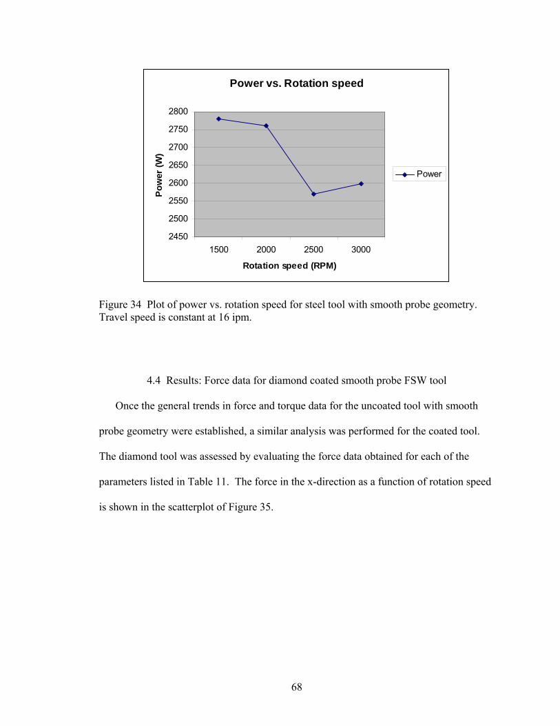
Power vs. Rotation speed
2450
2500
2550
2600
2650
2700
2750
2800
1500 2000 2500 3000
Rotation speed (RPM)
Pow
er (W
)Power
Figure 34 Plot of power vs. rotation speed for steel tool with smooth probe geometry. Travel speed is constant at 16 ipm.
4.4 Results: Force data for diamond coated smooth probe FSW tool
Once the general trends in force and torque data for the uncoated tool with smooth
probe geometry were established, a similar analysis was performed for the coated tool.
The diamond tool was assessed by evaluating the force data obtained for each of the
parameters listed in Table 11. The force in the x-direction as a function of rotation speed
is shown in the scatterplot of Figure 35.
68
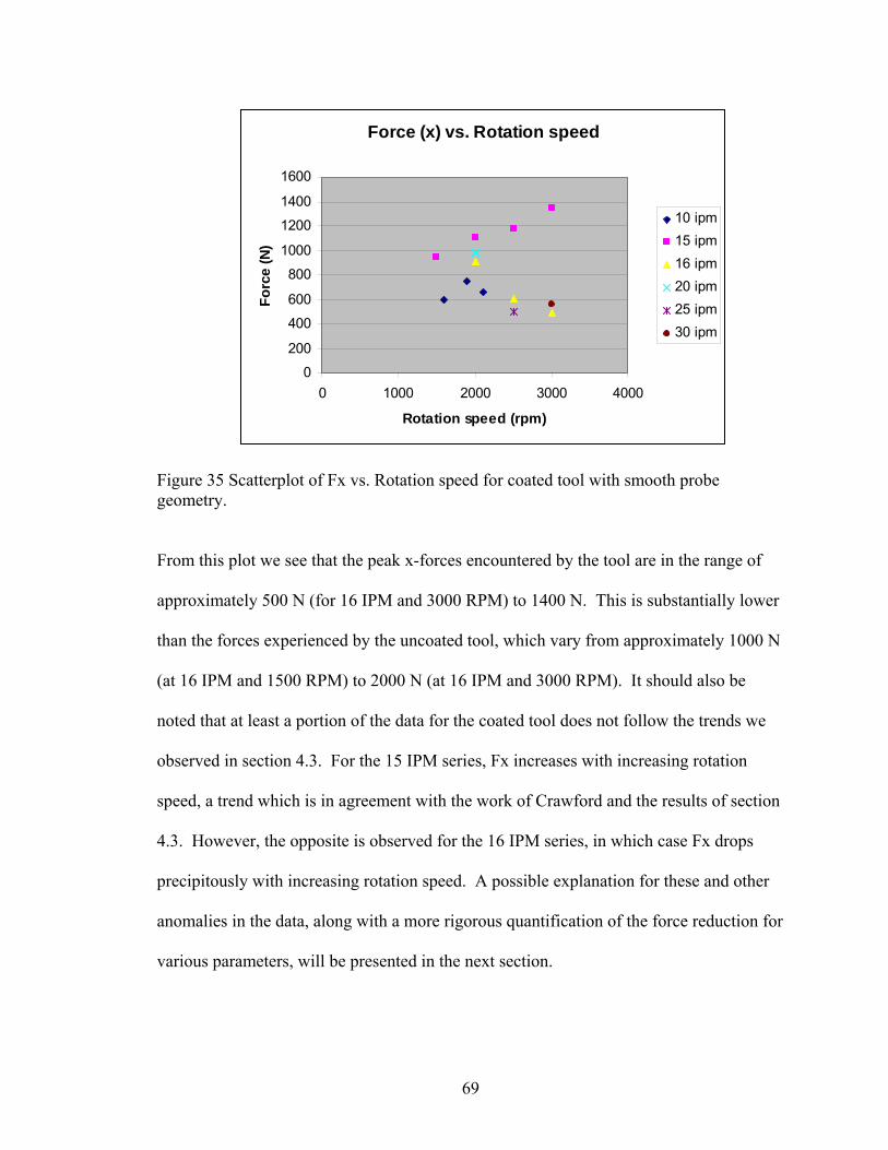
Force (x) vs. Rotation speed
0
200
400
600
800
1000
1200
1400
1600
0 1000 2000 3000 4000
Rotation speed (rpm)
Forc
e (N
)
10 ipm15 ipm16 ipm20 ipm25 ipm30 ipm
Figure 35 Scatterplot of Fx vs. Rotation speed for coated tool with smooth probe geometry.
From this plot we see that the peak x-forces encountered by the tool are in the range of
approximately 500 N (for 16 IPM and 3000 RPM) to 1400 N. This is substantially lower
than the forces experienced by the uncoated tool, which vary from approximately 1000 N
(at 16 IPM and 1500 RPM) to 2000 N (at 16 IPM and 3000 RPM). It should also be
noted that at least a portion of the data for the coated tool does not follow the trends we
observed in section 4.3. For the 15 IPM series, Fx increases with increasing rotation
speed, a trend which is in agreement with the work of Crawford and the results of section
4.3. However, the opposite is observed for the 16 IPM series, in which case Fx drops
precipitously with increasing rotation speed. A possible explanation for these and other
anomalies in the data, along with a more rigorous quantification of the force reduction for
various parameters, will be presented in the next section.
69
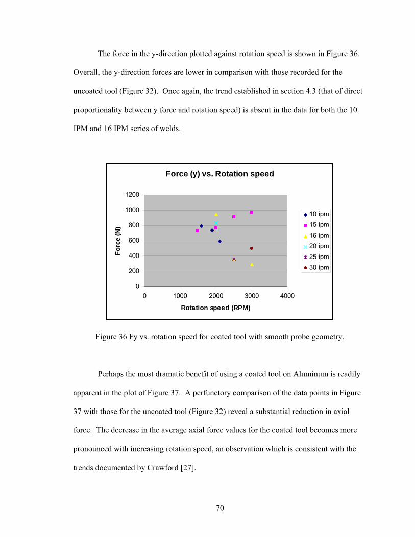
The force in the y-direction plotted against rotation speed is shown in Figure 36.
Overall, the y-direction forces are lower in comparison with those recorded for the
uncoated tool (Figure 32). Once again, the trend established in section 4.3 (that of direct
proportionality between y force and rotation speed) is absent in the data for both the 10
IPM and 16 IPM series of welds.
Force (y) vs. Rotation speed
0
200
400
600
800
1000
1200
0 1000 2000 3000 4000
Rotation speed (RPM)
Forc
e (N
)
10 ipm15 ipm16 ipm20 ipm25 ipm30 ipm
Figure 36 Fy vs. rotation speed for coated tool with smooth probe geometry.
Perhaps the most dramatic benefit of using a coated tool on Aluminum is readily
apparent in the plot of Figure 37. A perfunctory comparison of the data points in Figure
37 with those for the uncoated tool (Figure 32) reveal a substantial reduction in axial
force. The decrease in the average axial force values for the coated tool becomes more
pronounced with increasing rotation speed, an observation which is consistent with the
trends documented by Crawford [27].
70
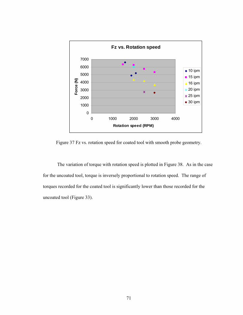
Fz vs. Rotation speed
0
1000
2000
3000
4000
5000
6000
7000
0 1000 2000 3000 4000
Rotation speed (RPM)
Forc
e (N
)10 ipm15 ipm16 ipm20 ipm25 ipm30 ipm
Figure 37 Fz vs. rotation speed for coated tool with smooth probe geometry.
The variation of torque with rotation speed is plotted in Figure 38. As in the case
for the uncoated tool, torque is inversely proportional to rotation speed. The range of
torques recorded for the coated tool is significantly lower than those recorded for the
uncoated tool (Figure 33).
71
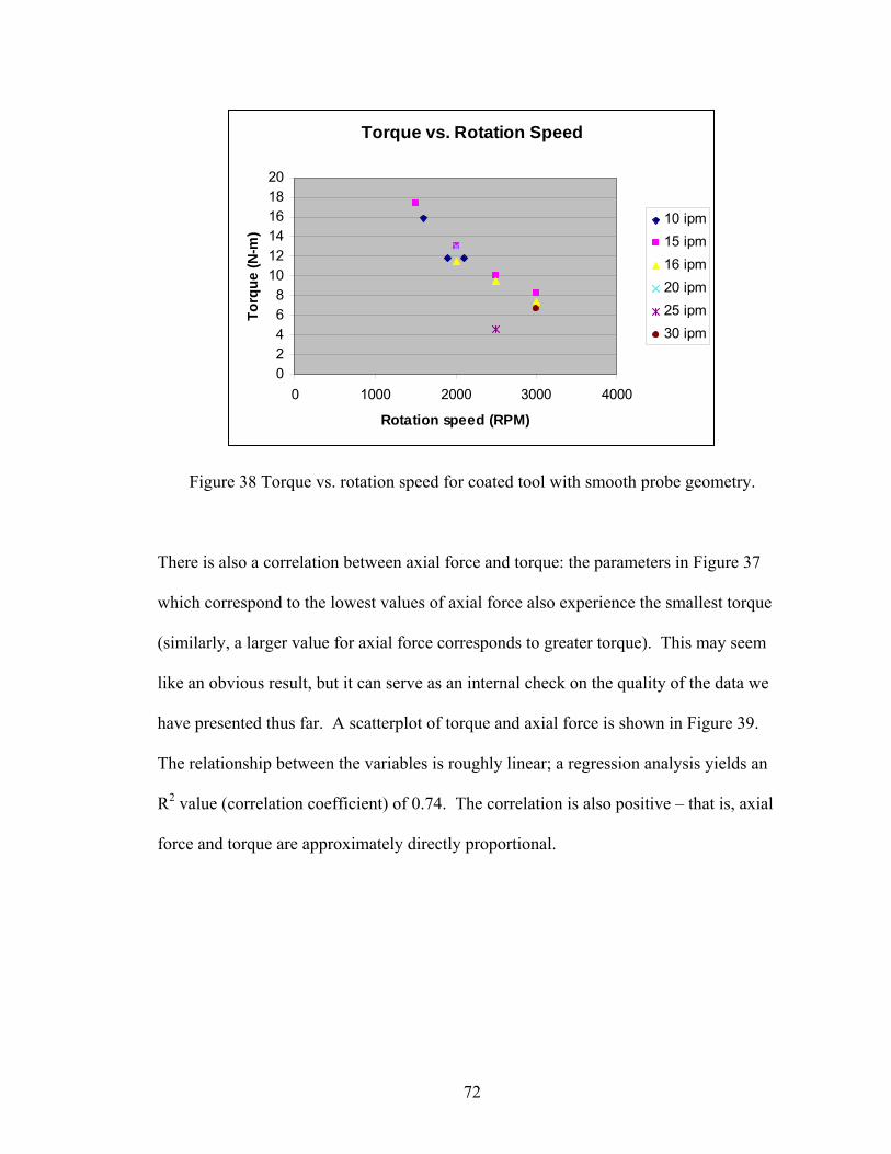
Torque vs. Rotation Speed
02468
101214161820
0 1000 2000 3000 4000
Rotation speed (RPM)
Torq
ue (N
-m)
10 ipm15 ipm16 ipm20 ipm25 ipm30 ipm
Figure 38 Torque vs. rotation speed for coated tool with smooth probe geometry.
There is also a correlation between axial force and torque: the parameters in Figure 37
which correspond to the lowest values of axial force also experience the smallest torque
(similarly, a larger value for axial force corresponds to greater torque). This may seem
like an obvious result, but it can serve as an internal check on the quality of the data we
have presented thus far. A scatterplot of torque and axial force is shown in Figure 39.
The relationship between the variables is roughly linear; a regression analysis yields an
R2 value (correlation coefficient) of 0.74. The correlation is also positive – that is, axial
force and torque are approximately directly proportional.
72
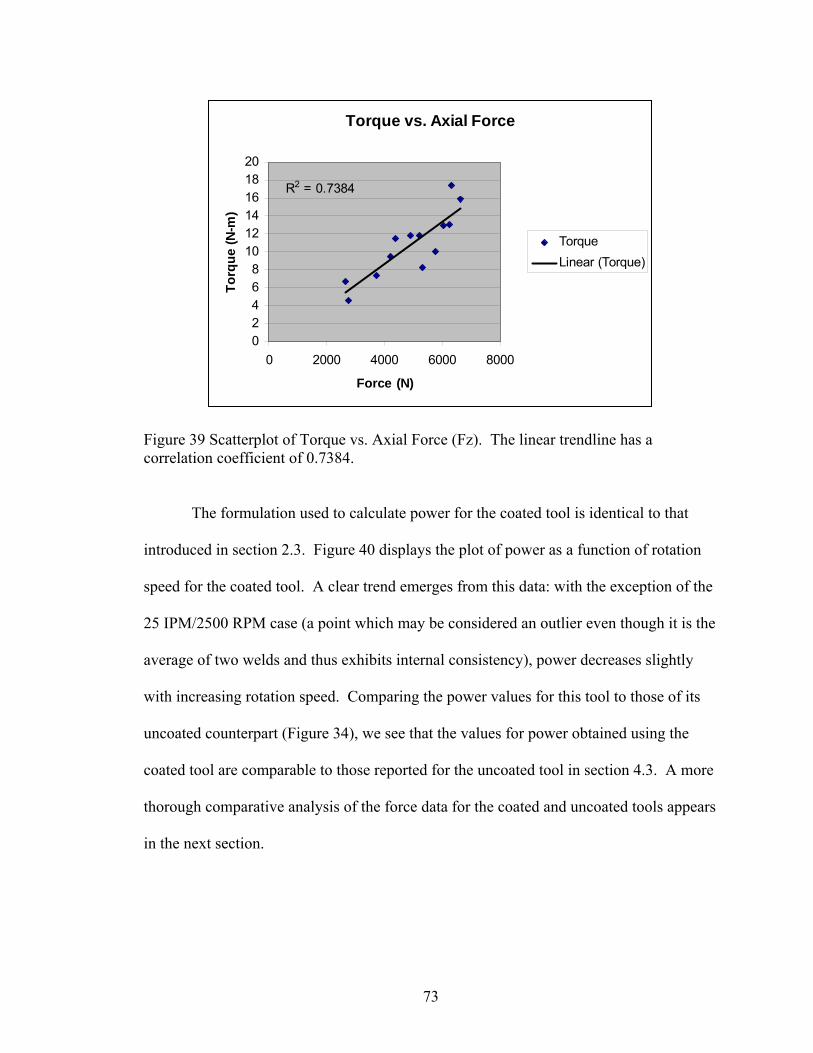
Torque vs. Axial Force
R2 = 0.7384
02468
101214161820
0 2000 4000 6000 8000
Force (N)
Torq
ue (N
-m)
TorqueLinear (Torque)
Figure 39 Scatterplot of Torque vs. Axial Force (Fz). The linear trendline has a correlation coefficient of 0.7384.
The formulation used to calculate power for the coated tool is identical to that
introduced in section 2.3. Figure 40 displays the plot of power as a function of rotation
speed for the coated tool. A clear trend emerges from this data: with the exception of the
25 IPM/2500 RPM case (a point which may be considered an outlier even though it is the
average of two welds and thus exhibits internal consistency), power decreases slightly
with increasing rotation speed. Comparing the power values for this tool to those of its
uncoated counterpart (Figure 34), we see that the values for power obtained using the
coated tool are comparable to those reported for the uncoated tool in section 4.3. A more
thorough comparative analysis of the force data for the coated and uncoated tools appears
in the next section.
73
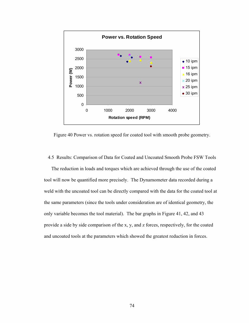
Power vs. Rotation Speed
0
500
1000
1500
2000
2500
3000
0 1000 2000 3000 4000
Rotation speed (RPM)
Pow
er (W
)
10 ipm15 ipm16 ipm20 ipm25 ipm30 ipm
Figure 40 Power vs. rotation speed for coated tool with smooth probe geometry.
4.5 Results: Comparison of Data for Coated and Uncoated Smooth Probe FSW Tools
The reduction in loads and torques which are achieved through the use of the coated
tool will now be quantified more precisely. The Dynamometer data recorded during a
weld with the uncoated tool can be directly compared with the data for the coated tool at
the same parameters (since the tools under consideration are of identical geometry, the
only variable becomes the tool material). The bar graphs in Figure 41, 42, and 43
provide a side by side comparison of the x, y, and z forces, respectively, for the coated
and uncoated tools at the parameters which showed the greatest reduction in forces.
74
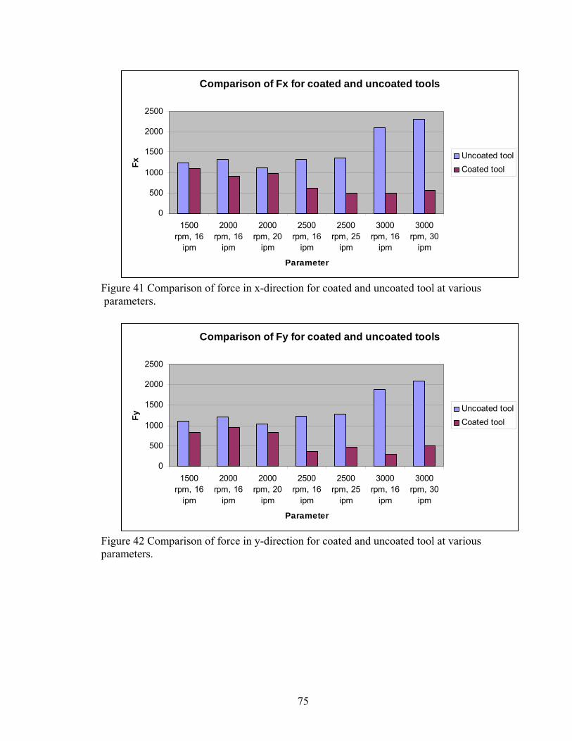
Comparison of Fx for coated and uncoated tools
0
500
1000
1500
2000
2500
1500rpm, 16
ipm
2000rpm, 16
ipm
2000rpm, 20
ipm
2500rpm, 16
ipm
2500rpm, 25
ipm
3000rpm, 16
ipm
3000rpm, 30
ipm
Parameter
Fx
Uncoated toolCoated tool
Figure 41 Comparison of force in x-direction for coated and uncoated tool at various parameters.
Comparison of Fy for coated and uncoated tools
0
500
1000
1500
2000
2500
1500rpm, 16
ipm
2000rpm, 16
ipm
2000rpm, 20
ipm
2500rpm, 16
ipm
2500rpm, 25
ipm
3000rpm, 16
ipm
3000rpm, 30
ipm
Parameter
Fy
Uncoated toolCoated tool
Figure 42 Comparison of force in y-direction for coated and uncoated tool at various parameters.
75
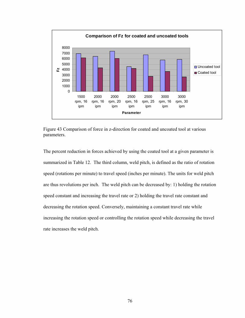
Comparison of Fz for coated and uncoated tools
010002000300040005000600070008000
1500rpm, 16
ipm
2000rpm, 16
ipm
2000rpm, 20
ipm
2500rpm, 16
ipm
2500rpm, 25
ipm
3000rpm, 16
ipm
3000rpm, 30
ipm
Parameter
Fz
Uncoated toolCoated tool
Figure 43 Comparison of force in z-direction for coated and uncoated tool at various parameters.
The percent reduction in forces achieved by using the coated tool at a given parameter is
summarized in Table 12. The third column, weld pitch, is defined as the ratio of rotation
speed (rotations per minute) to travel speed (inches per minute). The units for weld pitch
are thus revolutions per inch. The weld pitch can be decreased by: 1) holding the rotation
speed constant and increasing the travel rate or 2) holding the travel rate constant and
decreasing the rotation speed. Conversely, maintaining a constant travel rate while
increasing the rotation speed or controlling the rotation speed while decreasing the travel
rate increases the weld pitch.
76
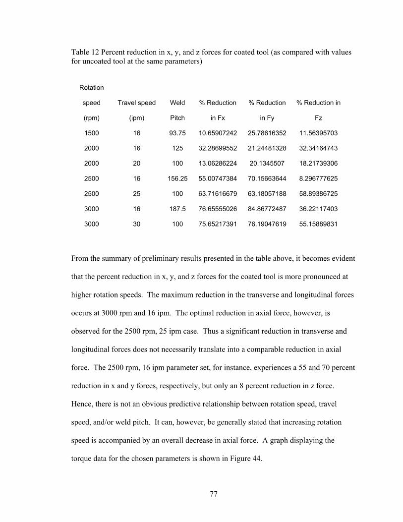
Table 12 Percent reduction in x, y, and z forces for coated tool (as compared with values for uncoated tool at the same parameters)
Rotation
speed
(rpm)
Travel speed
(ipm)
Weld
Pitch
% Reduction
in Fx
% Reduction
in Fy
% Reduction in
Fz
1500 16 93.75 10.65907242 25.78616352 11.56395703
2000 16 125 32.28699552 21.24481328 32.34164743
2000 20 100 13.06286224 20.1345507 18.21739306
2500 16 156.25 55.00747384 70.15663644 8.296777625
2500 25 100 63.71616679 63.18057188 58.89386725
3000 16 187.5 76.65555026 84.86772487 36.22117403
3000 30 100 75.65217391 76.19047619 55.15889831
From the summary of preliminary results presented in the table above, it becomes evident
that the percent reduction in x, y, and z forces for the coated tool is more pronounced at
higher rotation speeds. The maximum reduction in the transverse and longitudinal forces
occurs at 3000 rpm and 16 ipm. The optimal reduction in axial force, however, is
observed for the 2500 rpm, 25 ipm case. Thus a significant reduction in transverse and
longitudinal forces does not necessarily translate into a comparable reduction in axial
force. The 2500 rpm, 16 ipm parameter set, for instance, experiences a 55 and 70 percent
reduction in x and y forces, respectively, but only an 8 percent reduction in z force.
Hence, there is not an obvious predictive relationship between rotation speed, travel
speed, and/or weld pitch. It can, however, be generally stated that increasing rotation
speed is accompanied by an overall decrease in axial force. A graph displaying the
torque data for the chosen parameters is shown in Figure 44.
77
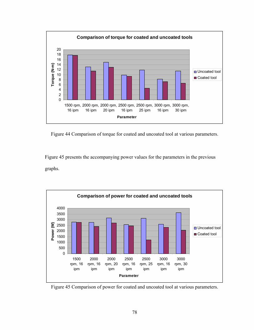
Comparison of torque for coated and uncoated tools
02468
101214161820
1500 rpm,16 ipm
2000 rpm,16 ipm
2000 rpm,20 ipm
2500 rpm,16 ipm
2500 rpm,25 ipm
3000 rpm,16 ipm
3000 rpm,30 ipm
Parameter
Torq
ue (N
-m)
Uncoated toolCoated tool
Figure 44 Comparison of torque for coated and uncoated tool at various parameters.
Figure 45 presents the accompanying power values for the parameters in the previous
graphs.
Comparison of power for coated and uncoated tools
0500
1000150020002500300035004000
1500rpm, 16
ipm
2000rpm, 16
ipm
2000rpm, 20
ipm
2500rpm, 16
ipm
2500rpm, 25
ipm
3000rpm, 16
ipm
3000rpm, 30
ipm
Parameter
Pow
er (W
)
Uncoated toolCoated tool
Figure 45 Comparison of power for coated and uncoated tool at various parameters.
78
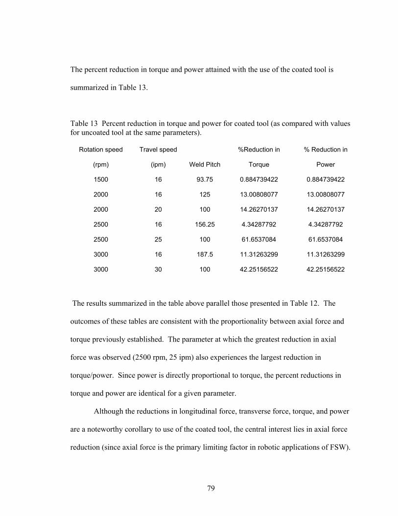
The percent reduction in torque and power attained with the use of the coated tool is
summarized in Table 13.
Table 13 Percent reduction in torque and power for coated tool (as compared with values for uncoated tool at the same parameters).
Rotation speed
(rpm)
Travel speed
(ipm) Weld Pitch
%Reduction in
Torque
% Reduction in
Power
1500 16 93.75 0.884739422 0.884739422
2000 16 125 13.00808077 13.00808077
2000 20 100 14.26270137 14.26270137
2500 16 156.25 4.34287792 4.34287792
2500 25 100 61.6537084 61.6537084
3000 16 187.5 11.31263299 11.31263299
3000 30 100 42.25156522 42.25156522
The results summarized in the table above parallel those presented in Table 12. The
outcomes of these tables are consistent with the proportionality between axial force and
torque previously established. The parameter at which the greatest reduction in axial
force was observed (2500 rpm, 25 ipm) also experiences the largest reduction in
torque/power. Since power is directly proportional to torque, the percent reductions in
torque and power are identical for a given parameter.
Although the reductions in longitudinal force, transverse force, torque, and power
are a noteworthy corollary to use of the coated tool, the central interest lies in axial force
reduction (since axial force is the primary limiting factor in robotic applications of FSW).
79
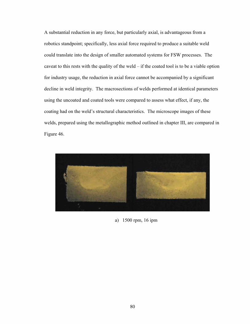
A substantial reduction in any force, but particularly axial, is advantageous from a
robotics standpoint; specifically, less axial force required to produce a suitable weld
could translate into the design of smaller automated systems for FSW processes. The
caveat to this rests with the quality of the weld – if the coated tool is to be a viable option
for industry usage, the reduction in axial force cannot be accompanied by a significant
decline in weld integrity. The macrosections of welds performed at identical parameters
using the uncoated and coated tools were compared to assess what effect, if any, the
coating had on the weld’s structural characteristics. The microscope images of these
welds, prepared using the metallographic method outlined in chapter III, are compared in
Figure 46.
a) 1500 rpm, 16 ipm
80
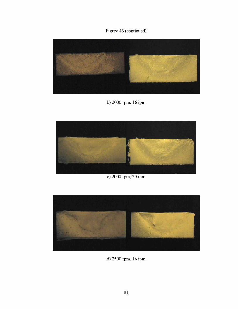
Figure 46 (continued)
b) 2000 rpm, 16 ipm
c) 2000 rpm, 20 ipm
d) 2500 rpm, 16 ipm
81
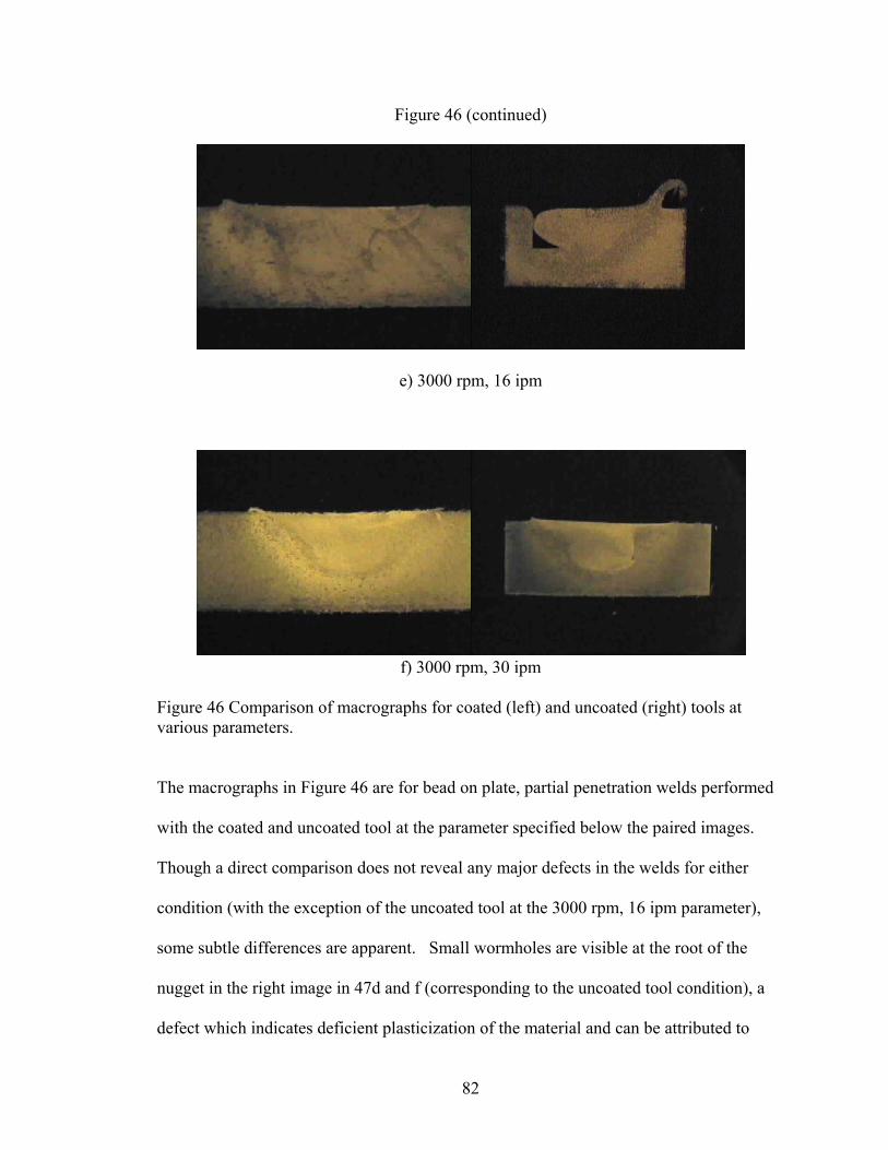
Figure 46 (continued)
e) 3000 rpm, 16 ipm
f) 3000 rpm, 30 ipm
Figure 46 Comparison of macrographs for coated (left) and uncoated (right) tools at various parameters.
The macrographs in Figure 46 are for bead on plate, partial penetration welds performed
with the coated and uncoated tool at the parameter specified below the paired images.
Though a direct comparison does not reveal any major defects in the welds for either
condition (with the exception of the uncoated tool at the 3000 rpm, 16 ipm parameter),
some subtle differences are apparent. Small wormholes are visible at the root of the
nugget in the right image in 47d and f (corresponding to the uncoated tool condition), a
defect which indicates deficient plasticization of the material and can be attributed to
82
excessive travel speed for a particular rotation speed. The heat affected zone (HAZ) also
differs slightly in size for the coated tools. The enlargement of the HAZ observed for the
macrographs on the left hand side of Figure 46 is related to the difference in thermal
conductivities between the tool and the workpiece, a disparity which will be evaluated
more thoroughly in the discussion which appears in the final section of this chapter.
The material properties of Molybdenum (the base material upon which the
diamond coating is deposited) and the effect they may exert on the welding process must
also be considered. Though ideal as a CVD coating substrate, Molybdenum tools have a
tendency to flake during machining. Initial welds with the coated tool resulted in a
surface with hard Aluminum shavings dispersed along the weld path. This surface
structure was distinct from the flash which sometimes accumulates at the perimeter of the
weld path (indicating overheating), thus pointing toward a problem with material
interface between the tool and workpiece rather than parameter selection. However, once
the rotation speed was increased to 1500 rpm or greater, this flakiness disappeared and
was replaced by a smooth, mirror-like finish which ran the length of the weld. Figure 47
shows a comparison of the surface texture for selected welds using the coated and
uncoated tools. In cases a) and b), the welds produced using the coated and uncoated tool
are comparable in surface quality. However, the macrographs previously presented in
Figure 46 reveal a wormhole in the weld at parameter b using the uncoated tool; the weld
with the coated tool is free of defects at this parameter. For cases c), d), and e), the
surface structure of the welds made using the coated tool are superior to those made using
the uncoated tool. In c) and d), both of the welds being compared have flash, but the
surface of the weld performed using the coated tool has a significantly smoother texture.
83
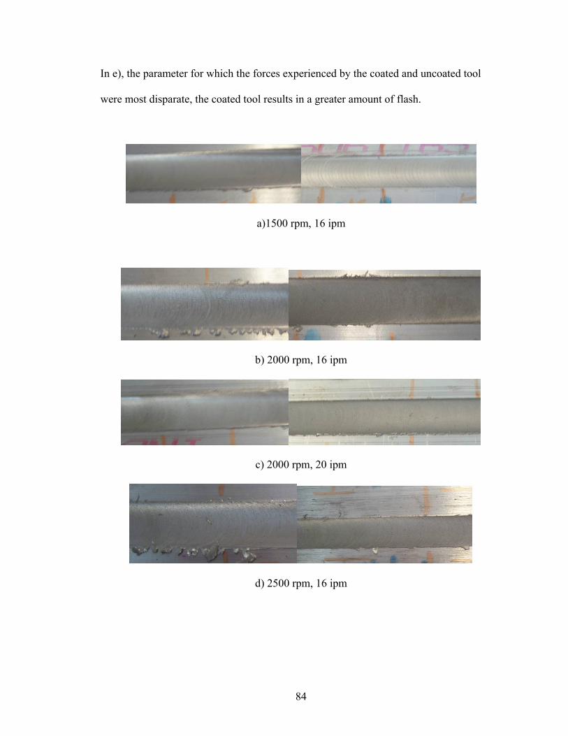
In e), the parameter for which the forces experienced by the coated and uncoated tool
were most disparate, the coated tool results in a greater amount of flash.
a)1500 rpm, 16 ipm
b) 2000 rpm, 16 ipm
c) 2000 rpm, 20 ipm
d) 2500 rpm, 16 ipm
84
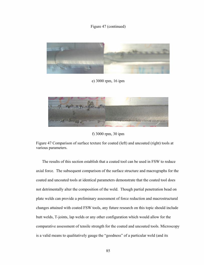
Figure 47 (continued)
e) 3000 rpm, 16 ipm
f) 3000 rpm, 30 ipm
Figure 47 Comparison of surface texture for coated (left) and uncoated (right) tools at various parameters.
The results of this section establish that a coated tool can be used in FSW to reduce
axial force. The subsequent comparison of the surface structure and macrographs for the
coated and uncoated tools at identical parameters demonstrate that the coated tool does
not detrimentally alter the composition of the weld. Though partial penetration bead on
plate welds can provide a preliminary assessment of force reduction and macrostructural
changes attained with coated FSW tools, any future research on this topic should include
butt welds, T-joints, lap welds or any other configuration which would allow for the
comparative assessment of tensile strength for the coated and uncoated tools. Microscopy
is a valid means to qualitatively gauge the “goodness” of a particular weld (and its
85
importance should not be discounted), but strength testing is the easiest method by which
to generate quantitative data. A move to a weld configuration with a true joint line,
however, necessitates redesign of the tool. A smooth cylindrical probe does not produce
enough downward vertical flow to make a strong weld; hence alternate geometries which
incorporate more complex features such as threads, flutes, or flares to enhance vertical
flow must be considered. Features such as those mentioned, however, introduce a stress
concentration to a Molybdenum substrate which is already susceptible to shear stresses.
As expected based on the material properties of Molybdenum, all attempts at the use of a
threaded diamond coated probe resulted in failure at the entrance to the material. Thus
for probes with features, a less brittle Molybdenum alloy (or another substrate altogether)
should be considered as the tool base material.
4.6 Analysis and Conclusions
The CVD diamond coating has a number of properties which suggest it would aid
in the joining of materials through Friction Stir Welding (FSW). The hardness of the
diamond coating makes it a good candidate for the welding of superabrasive materials
such as MMCs. Diamond is the hardest known material (100 on the Rockwell Hardness
Scale); consequently, it is expected that a diamond-coated tool would be resistant to the
tool wear which plagues conventional tools in MMC welding [29]. This hardness may
also contribute to the reduction in axial force, which has the potential to enhance robotic
FSW applications. Additionally, diamond has the highest longitudinal sound velocity
[29]. Since one potential method of wear detection is the analysis of acoustic emissions
by Fourier transforms, this property could be exploited to compare the rate of tool wear
86
for the diamond-coated Molybdenum tool with that of its steel counterpart. The high
thermal conductivity of the diamond coating (20W/cm/oC) may enable it to function as a
heat sink, a characteristic which could prove an asset in high-speed welding processes
where the high-temperatures attained impose limitations on traditional steel tools [29].
Although diamond is largely inert, it does interact with carbon-based materials; this
places restrictions on the materials which can be joined using the proposed tool. The
carbon content of iron materials, such as steel, could result in the dissolution of the
diamond coating [13]. This tendency to dissolve diamond, coupled with the inability of
steel to withstand the CVD chamber, makes steel a poor choice for a base tool material in
this investigation. Titanium and its alloys are also unweldable with the diamond-coated
Molybdenum tool because Titanium interacts with diamond to form carbides [13]. To
prevent this interaction, a shielding mechanism must be devised; the apparatus in the
Vanderbilt Welding Laboratory is not currently set up to accommodate such a procedure.
Aluminum and Aluminum MMCs appear to be the best choices for joining materials
when using the CVD Molybdenum tool.
Returning to the concept of heat transfer, Roy, Nandan, and Debroy propose the
factor f, a dimensionless ratio that characterizes how the heat generated by the tool is
transmitted between the tool and the workpiece (analogous to the process efficiency
factor in arc welding) [28]. The factor f is expressed as:
f = [(kρCp)W]1/2 / [(kρCp)T]1/2 (1)
where
k = thermal conductivity
ρ = density of the material
87
Cp = specific heat at constant pressure [28]
The subscripts W and T refer to the workpiece and tool, respectively.
For the coated case, we will assume the tool has the properties of CVD diamond, since
the coating (assuming it does not wear off during the process) is what actually contacts
the workpiece material (not the Molybdenum substrate). For diamond at room
temperature, k =2000 W/m-K, ρ =3500 kg/m3 , and Cp = 0.4715 J/g-K. The material
properties of CVD diamond are nearly identical to those of diamond (the variation is less
than 0.1%), so substituting the values for diamond into equation (1) is justified in this
instance [30]. For Aluminum Alloy 6061 in the T6 condition at room temperature, k =
195 W/m-K, ρ = 2705 kg/m3, and Cp = 0.87 J/g-K [4]. Substituting these values into the
Roy equation, we obtain 0.3729. This analysis, though simplistic since k and Cp vary
nonlinearly with temperature, predicts that only 37 percent of the heat generated at the
tool/workpiece interface will be transported between the tool and the workpiece. This
suggests that since a large portion of the heat will be going into the tool, it must be
compensated for by rotating the tool at higher spindle speeds. This lends support to the
idea that the Molybdenum-coated diamond tool is better-suited for high-speed welding
than welding at slower rotation speeds.
The f factor of Roy et al. can be used to evaluate the distribution of heat between
the tool and the workpiece for a range of welding temperatures. The thermophysical
properties of Aluminum 6061 as a function of temperature are listed in Table 14 (adapted
from reference 31). The temperatures considered are consistent with those incurred in a
solid-state process, ranging from 25 oC (room temperature) to 600 oC (near the melting
point).
88
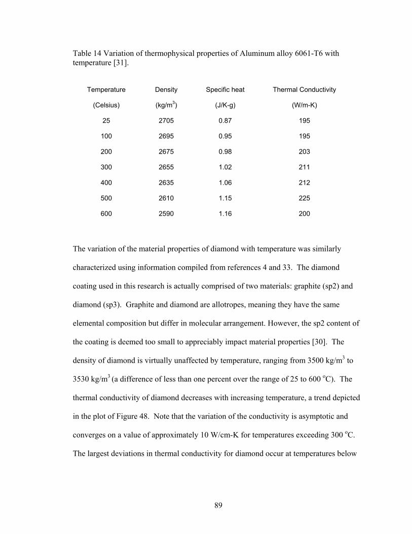
Table 14 Variation of thermophysical properties of Aluminum alloy 6061-T6 with temperature [31].
Temperature
(Celsius)
Density
(kg/m3)
Specific heat
(J/K-g)
Thermal Conductivity
(W/m-K)
25 2705 0.87 195
100 2695 0.95 195
200 2675 0.98 203
300 2655 1.02 211
400 2635 1.06 212
500 2610 1.15 225
600 2590 1.16 200
The variation of the material properties of diamond with temperature was similarly
characterized using information compiled from references 4 and 33. The diamond
coating used in this research is actually comprised of two materials: graphite (sp2) and
diamond (sp3). Graphite and diamond are allotropes, meaning they have the same
elemental composition but differ in molecular arrangement. However, the sp2 content of
the coating is deemed too small to appreciably impact material properties [30]. The
density of diamond is virtually unaffected by temperature, ranging from 3500 kg/m3 to
3530 kg/m3 (a difference of less than one percent over the range of 25 to 600 oC). The
thermal conductivity of diamond decreases with increasing temperature, a trend depicted
in the plot of Figure 48. Note that the variation of the conductivity is asymptotic and
converges on a value of approximately 10 W/cm-K for temperatures exceeding 300 oC.
The largest deviations in thermal conductivity for diamond occur at temperatures below
89
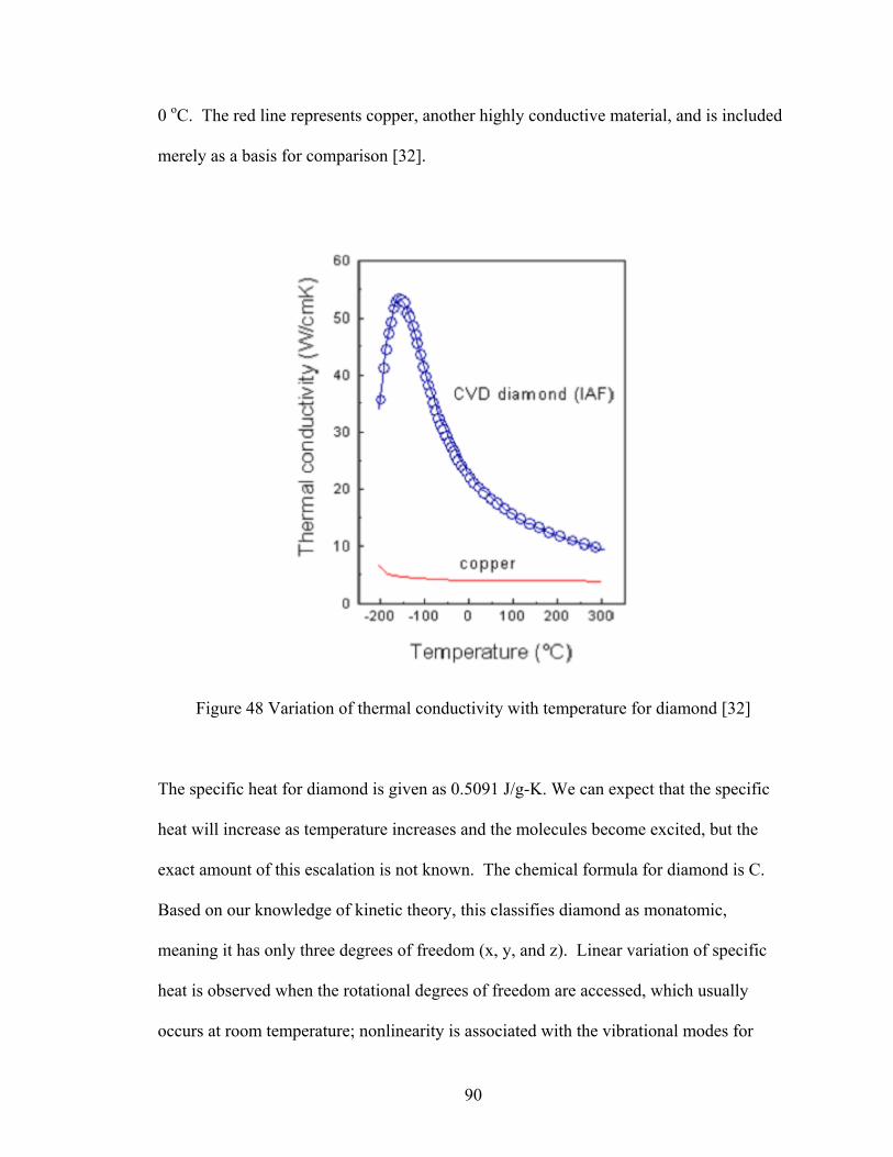
0 oC. The red line represents copper, another highly conductive material, and is included
merely as a basis for comparison [32].
Figure 48 Variation of thermal conductivity with temperature for diamond [32]
The specific heat for diamond is given as 0.5091 J/g-K. We can expect that the specific
heat will increase as temperature increases and the molecules become excited, but the
exact amount of this escalation is not known. The chemical formula for diamond is C.
Based on our knowledge of kinetic theory, this classifies diamond as monatomic,
meaning it has only three degrees of freedom (x, y, and z). Linear variation of specific
heat is observed when the rotational degrees of freedom are accessed, which usually
occurs at room temperature; nonlinearity is associated with the vibrational modes for
90
higher temperatures (greater than 600 K). Since diamond only has three translational
degrees of freedom, it is reasonable to assume that the specific heat of diamond at
constant pressure, Cp, is constant with temperature.
Returning to equation (1), it is apparent that the denominator of the dimensionless
constant f will change only marginally with temperature. Increasing the rotational speed
of the FSW tool so that the temperature of the Aluminum edges closer to the melting
point of the workpiece could increase the f value to as much as 0.49. This reduces the
heat transfer disparity between the tool and the workpiece, perhaps resulting in an
improved joint.
91
CHAPTER V
PARAMETERIZATION OF FRICTION STIR WELDING OF AL 6061 AND AL 6061/SIC/17.5P FOR TRIVEX TOOL
As outlined in the introduction, one of the goals of this research is to reduce the
axial force necessary to produce a structurally sound friction stir weld. In chapter IV, this
force reduction was accomplished by means of layering a diamond coating on the smooth
probe of an FSW tool. Though the results of the previous chapter established the efficacy
of this method, it has two major disadvantages from an industry/cost standpoint.
Diamond is an expensive coating material whose use is usually reserved for situations in
which the potential benefits justify the extra cost (it remains to be seen if FSW of Al
6061 fits this criterion). Additionally, the susceptibility of the Molybdenum substrate to
shear stress precludes the exploration of more complex probe geometries and joint
configurations. A less expensive and timely alternative to coatings as a means of force
reduction is the use of the Trivex tool, a design patented by The Welding Institute (TWI)
in February 2003 [33]. This chapter will focus on the application of the Trivex tool in
butt welding of Al 6061 and Al 6061/SiC/17.5p (an Aluminum Metal Matrix Composite).
Force data, microscopy, results of tensile tests, and (in the case of the Al-MMCs)
periodic measurements of tool wear will be presented. Based on these collective
outcomes, an operating window for the use of the Trivex tool in butt welding of these two
materials was established.
92
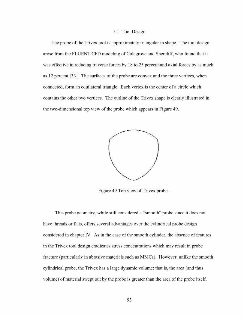
5.1 Tool Design
The probe of the Trivex tool is approximately triangular in shape. The tool design
arose from the FLUENT CFD modeling of Colegrove and Shercliff, who found that it
was effective in reducing traverse forces by 18 to 25 percent and axial forces by as much
as 12 percent [33]. The surfaces of the probe are convex and the three vertices, when
connected, form an equilateral triangle. Each vertex is the center of a circle which
contains the other two vertices. The outline of the Trivex shape is clearly illustrated in
the two-dimensional top view of the probe which appears in Figure 49.
Figure 49 Top view of Trivex probe.
This probe geometry, while still considered a “smooth” probe since it does not
have threads or flats, offers several advantages over the cylindrical probe design
considered in chapter IV. As in the case of the smooth cylinder, the absence of features
in the Trivex tool design eradicates stress concentrations which may result in probe
fracture (particularly in abrasive materials such as MMCs). However, unlike the smooth
cylindrical probe, the Trivex has a large dynamic volume; that is, the area (and thus
volume) of material swept out by the probe is greater than the area of the probe itself.
93
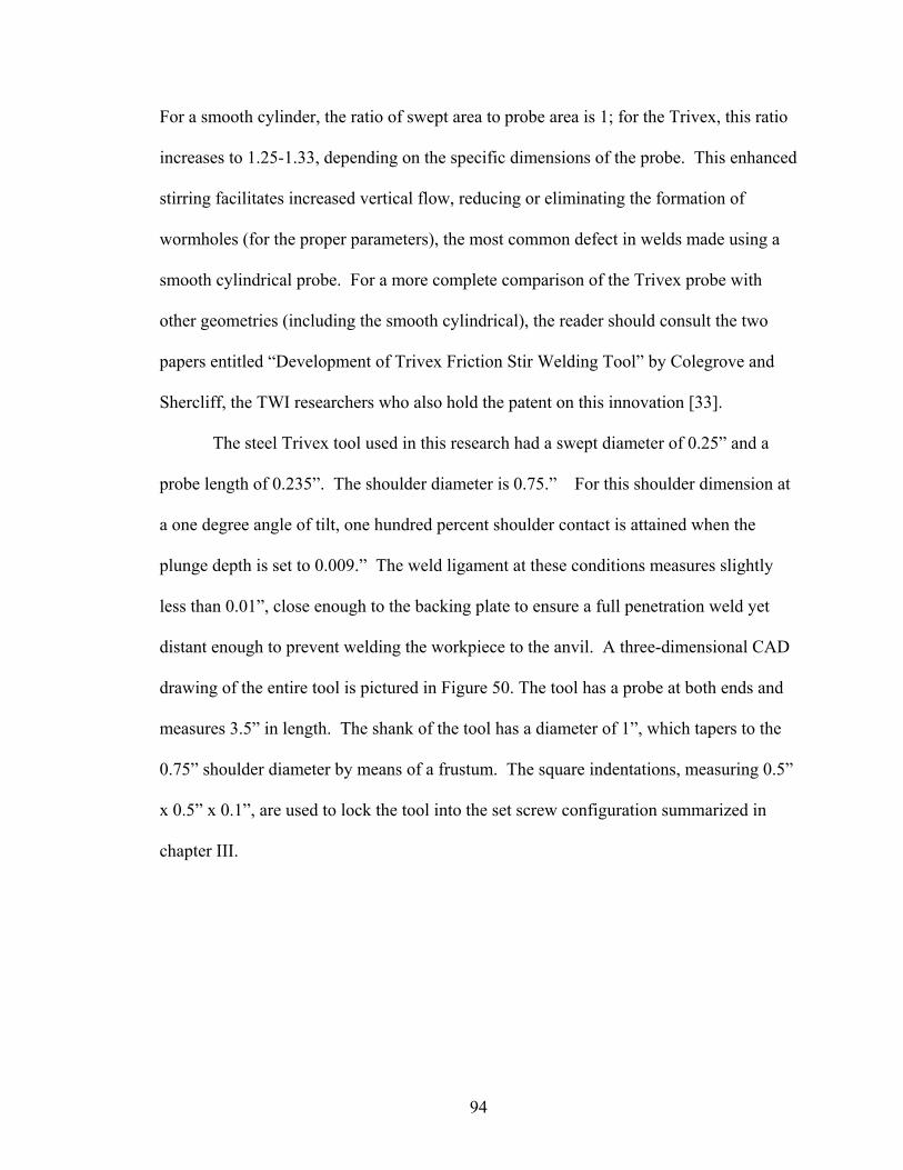
For a smooth cylinder, the ratio of swept area to probe area is 1; for the Trivex, this ratio
increases to 1.25-1.33, depending on the specific dimensions of the probe. This enhanced
stirring facilitates increased vertical flow, reducing or eliminating the formation of
wormholes (for the proper parameters), the most common defect in welds made using a
smooth cylindrical probe. For a more complete comparison of the Trivex probe with
other geometries (including the smooth cylindrical), the reader should consult the two
papers entitled “Development of Trivex Friction Stir Welding Tool” by Colegrove and
Shercliff, the TWI researchers who also hold the patent on this innovation [33].
The steel Trivex tool used in this research had a swept diameter of 0.25” and a
probe length of 0.235”. The shoulder diameter is 0.75.” For this shoulder dimension at
a one degree angle of tilt, one hundred percent shoulder contact is attained when the
plunge depth is set to 0.009.” The weld ligament at these conditions measures slightly
less than 0.01”, close enough to the backing plate to ensure a full penetration weld yet
distant enough to prevent welding the workpiece to the anvil. A three-dimensional CAD
drawing of the entire tool is pictured in Figure 50. The tool has a probe at both ends and
measures 3.5” in length. The shank of the tool has a diameter of 1”, which tapers to the
0.75” shoulder diameter by means of a frustum. The square indentations, measuring 0.5”
x 0.5” x 0.1”, are used to lock the tool into the set screw configuration summarized in
chapter III.
94
Figure 50 A side view CAD-rendered image of the Trivex tool used in this research.
5.2 Parameter selection for butt welding of Al 6061
The parameters for butt welding of Al 6061 (the unreinforced alloy) were again
chosen based on the operational constraints of the laboratory apparatus during the period
the research was conducted. The maximum operating speeds of the various motors are
summarized in Table 15.
Table 15 Maximum operating speeds for FSW apparatus motors at time of Trivex tool research.
Motor
Maximum operating
speed
Spindle 2500 rpm
Traverse 14 ipm
Lateral 2 ipm
Vertical 5 ipm
The corresponding weld matrix for the Trivex tool on Aluminum 6061 appears in Table
16. An “x” indicates parameters for which welds were performed. A “/” identifies
parameter sets which were unsuitable due to a mismatch in travel/spindle speed. For
95
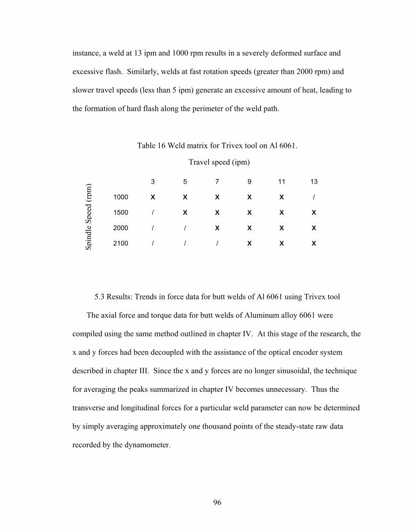
instance, a weld at 13 ipm and 1000 rpm results in a severely deformed surface and
excessive flash. Similarly, welds at fast rotation speeds (greater than 2000 rpm) and
slower travel speeds (less than 5 ipm) generate an excessive amount of heat, leading to
the formation of hard flash along the perimeter of the weld path.
Table 16 Weld matrix for Trivex tool on Al 6061.
Travel speed (ipm)
3 5 7 9 11 13
1000 X X X X X /
1500 / X X X X X
2000 / / X X X X
2100 / / / X X X Spin
dle
Spee
d (r
pm)
5.3 Results: Trends in force data for butt welds of Al 6061 using Trivex tool
The axial force and torque data for butt welds of Aluminum alloy 6061 were
compiled using the same method outlined in chapter IV. At this stage of the research, the
x and y forces had been decoupled with the assistance of the optical encoder system
described in chapter III. Since the x and y forces are no longer sinusoidal, the technique
for averaging the peaks summarized in chapter IV becomes unnecessary. Thus the
transverse and longitudinal forces for a particular weld parameter can now be determined
by simply averaging approximately one thousand points of the steady-state raw data
recorded by the dynamometer.
96
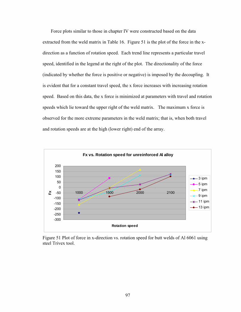
Force plots similar to those in chapter IV were constructed based on the data
extracted from the weld matrix in Table 16. Figure 51 is the plot of the force in the x-
direction as a function of rotation speed. Each trend line represents a particular travel
speed, identified in the legend at the right of the plot. The directionality of the force
(indicated by whether the force is positive or negative) is imposed by the decoupling. It
is evident that for a constant travel speed, the x force increases with increasing rotation
speed. Based on this data, the x force is minimized at parameters with travel and rotation
speeds which lie toward the upper right of the weld matrix. The maximum x force is
observed for the more extreme parameters in the weld matrix; that is, when both travel
and rotation speeds are at the high (lower right) end of the array.
Fx vs. Rotation speed for unreinforced Al alloy
-300-250-200-150-100-50
050
100150200
1000 1500 2000 2100
Rotation speed
3 ipm5 ipm7 ipm
Fx 9 ipm11 ipm13 ipm
Figure 51 Plot of force in x-direction vs. rotation speed for butt welds of Al 6061 using steel Trivex tool.
97
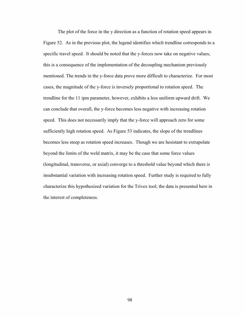
The plot of the force in the y direction as a function of rotation speed appears in
Figure 52. As in the previous plot, the legend identifies which trendline corresponds to a
specific travel speed. It should be noted that the y-forces now take on negative values;
this is a consequence of the implementation of the decoupling mechanism previously
mentioned. The trends in the y-force data prove more difficult to characterize. For most
cases, the magnitude of the y-force is inversely proportional to rotation speed. The
trendline for the 11 ipm parameter, however, exhibits a less uniform upward drift. We
can conclude that overall, the y-force becomes less negative with increasing rotation
speed. This does not necessarily imply that the y-force will approach zero for some
sufficiently high rotation speed. As Figure 53 indicates, the slope of the trendlines
becomes less steep as rotation speed increases. Though we are hesistant to extrapolate
beyond the limits of the weld matrix, it may be the case that some force values
(longitudinal, transverse, or axial) converge to a threshold value beyond which there is
insubstantial variation with increasing rotation speed. Further study is required to fully
characterize this hypothesized variation for the Trivex tool; the data is presented here in
the interest of completeness.
98
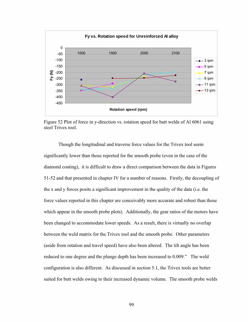
Fy vs. Rotation speed for Unreinforced Al alloy
-450
-400-350
-300
-250-200
-150
-100-50
01000 1500 2000 2100
Rotation speed (rpm)
Fy (N
)
3 ipm5 ipm7 ipm9 ipm11 ipm13 ipm
Figure 52 Plot of force in y-direction vs. rotation speed for butt welds of Al 6061 using steel Trivex tool.
Though the longitudinal and traverse force values for the Trivex tool seem
significantly lower than those reported for the smooth probe (even in the case of the
diamond coating), it is difficult to draw a direct comparison between the data in Figures
51-52 and that presented in chapter IV for a number of reasons. Firstly, the decoupling of
the x and y forces posits a significant improvement in the quality of the data (i.e. the
force values reported in this chapter are conceivably more accurate and robust than those
which appear in the smooth probe plots). Additionally, the gear ratios of the motors have
been changed to accommodate lower speeds. As a result, there is virtually no overlap
between the weld matrix for the Trivex tool and the smooth probe. Other parameters
(aside from rotation and travel speed) have also been altered. The tilt angle has been
reduced to one degree and the plunge depth has been increased to 0.009.” The weld
configuration is also different. As discussed in section 5.1, the Trivex tools are better
suited for butt welds owing to their increased dynamic volume. The smooth probe welds
99
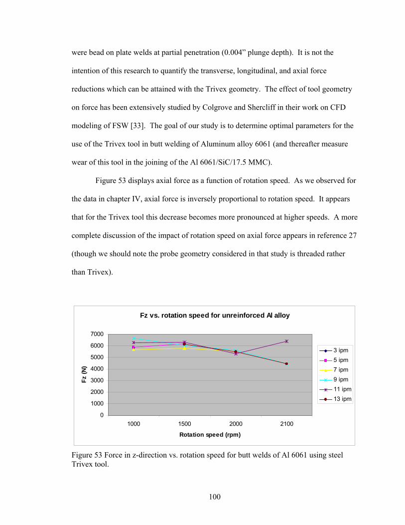
were bead on plate welds at partial penetration (0.004” plunge depth). It is not the
intention of this research to quantify the transverse, longitudinal, and axial force
reductions which can be attained with the Trivex geometry. The effect of tool geometry
on force has been extensively studied by Colgrove and Shercliff in their work on CFD
modeling of FSW [33]. The goal of our study is to determine optimal parameters for the
use of the Trivex tool in butt welding of Aluminum alloy 6061 (and thereafter measure
wear of this tool in the joining of the Al 6061/SiC/17.5 MMC).
Figure 53 displays axial force as a function of rotation speed. As we observed for
the data in chapter IV, axial force is inversely proportional to rotation speed. It appears
that for the Trivex tool this decrease becomes more pronounced at higher speeds. A more
complete discussion of the impact of rotation speed on axial force appears in reference 27
(though we should note the probe geometry considered in that study is threaded rather
than Trivex).
Fz vs. rotation speed for unreinforced Al alloy
0
1000
2000
3000
4000
5000
6000
7000
1000 1500 2000 2100
Rotation speed (rpm)
Fz (N
)
3 ipm5 ipm7 ipm9 ipm11 ipm13 ipm
Figure 53 Force in z-direction vs. rotation speed for butt welds of Al 6061 using steel Trivex tool.
100
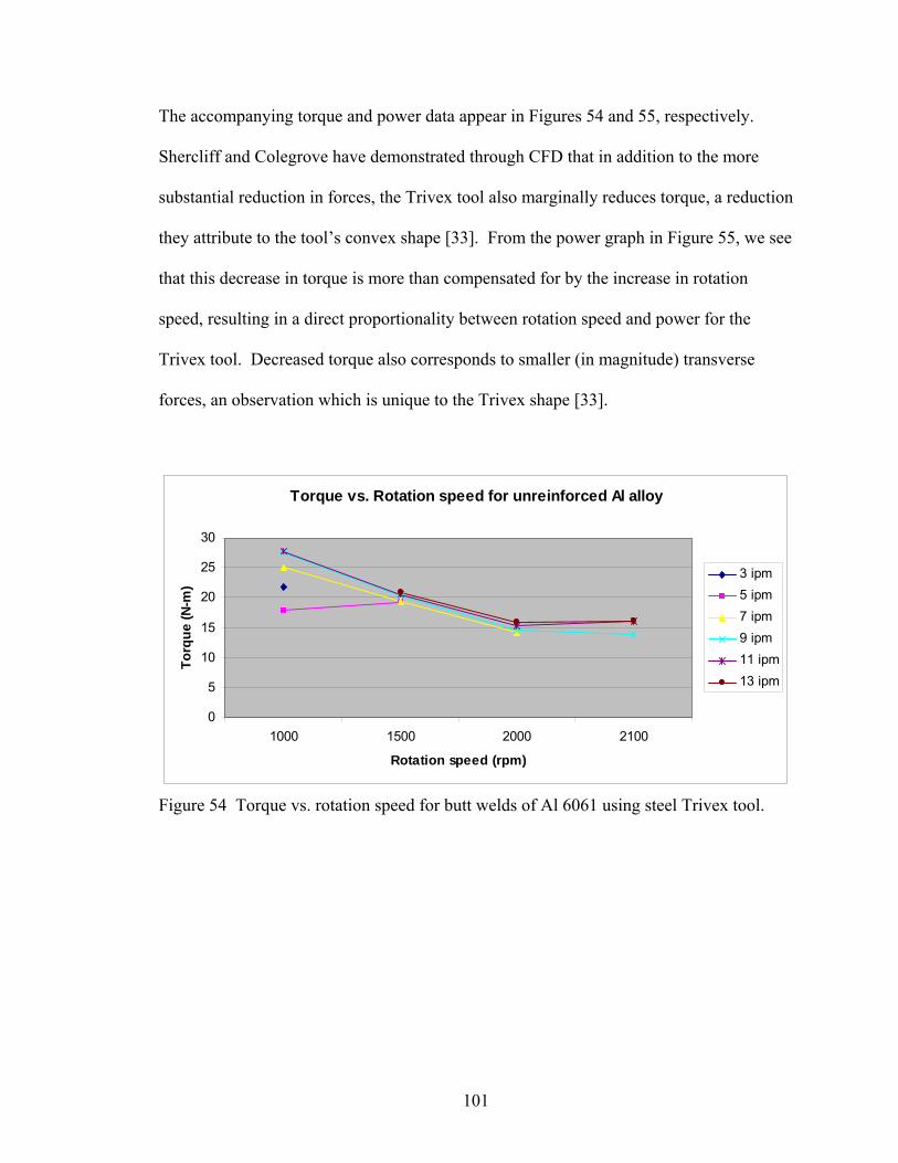
The accompanying torque and power data appear in Figures 54 and 55, respectively.
Shercliff and Colegrove have demonstrated through CFD that in addition to the more
substantial reduction in forces, the Trivex tool also marginally reduces torque, a reduction
they attribute to the tool’s convex shape [33]. From the power graph in Figure 55, we see
that this decrease in torque is more than compensated for by the increase in rotation
speed, resulting in a direct proportionality between rotation speed and power for the
Trivex tool. Decreased torque also corresponds to smaller (in magnitude) transverse
forces, an observation which is unique to the Trivex shape [33].
Torque vs. Rotation speed for unreinforced Al alloy
0
5
10
15
20
25
30
1000 1500 2000 2100
Rotation speed (rpm)
Torq
ue (N
-m)
3 ipm5 ipm7 ipm9 ipm11 ipm13 ipm
Figure 54 Torque vs. rotation speed for butt welds of Al 6061 using steel Trivex tool.
101
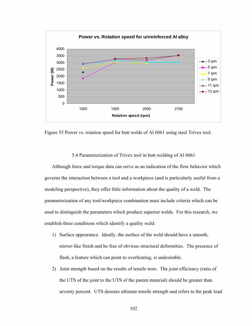
Power vs. Rotation speed for unreinforced Al alloy
0
500
1000
1500
2000
2500
3000
3500
4000
1000 1500 2000 2100
Rotation speed (rpm)
Pow
er (W
)
3 ipm5 ipm7 ipm9 ipm11 ipm13 ipm
Figure 55 Power vs. rotation speed for butt welds of Al 6061 using steel Trivex tool.
5.4 Parameterization of Trivex tool in butt welding of Al 6061
Although force and torque data can serve as an indication of the flow behavior which
governs the interaction between a tool and a workpiece (and is particularly useful from a
modeling perspective), they offer little information about the quality of a weld. The
parameterization of any tool/workpiece combination must include criteria which can be
used to distinguish the parameters which produce superior welds. For this research, we
establish three conditions which identify a quality weld:
1) Surface appearance. Ideally, the surface of the weld should have a smooth,
mirror-like finish and be free of obvious structural deformities. The presence of
flash, a feature which can point to overheating, is undesirable.
2) Joint strength based on the results of tensile tests. The joint efficiency (ratio of
the UTS of the joint to the UTS of the parent material) should be greater than
seventy percent. UTS denotes ultimate tensile strength and refers to the peak load
102
(normalized with respect to the cross sectional area of the tensile sample)
the specimen is able to withstand during the course of testing. Though not
requisite, it is additionally desirable that the specimen fracture in the parent
material (rather than along the joint line).
3) Microscopy. When the weld cross sections are etched and analyzed under a
microscope, they should be absent of defects (including, but not limited to,
cracking, wormholes, voids, and/or hooking). In most cases, a poor tensile test
result indicates the presence of a defect. A high joint efficiency, however, does
not necessarily preclude the existence of these structural imperfections. We are
cautious not to understate the importance of cross-sectioning all samples, even
those with favorable tensile test results.
Based on the criteria outlined above, an operating window for the use of the Trivex tool
in the butt welding of Al 6061 was established. This window is designated by the shaded
region of the weld matrix in Table 17 (at least one weld at each of the shaded parameters
was deemed a “good” weld).
103
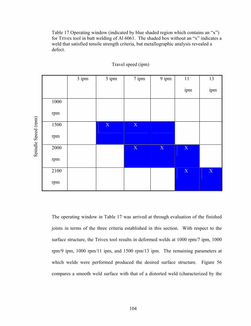
Table 17 Operating window (indicated by blue shaded region which contains an “x”) for Trivex tool in butt welding of Al 6061. The shaded box without an “x” indicates a weld that satisfied tensile strength criteria, but metallographic analysis revealed a defect.
Travel speed (ipm)
3 ipm 5 ipm 7 ipm 9 ipm 11
ipm
13
ipm
1000
rpm
1500
rpm
X X
2000
rpm
X X X
2100
rpm
X X
Spin
dle
Spee
d (r
pm)
The operating window in Table 17 was arrived at through evaluation of the finished
joints in terms of the three criteria established in this section. With respect to the
surface structure, the Trivex tool results in deformed welds at 1000 rpm/7 ipm, 1000
rpm/9 ipm, 1000 rpm/11 ipm, and 1500 rpm/13 ipm. The remaining parameters at
which welds were performed produced the desired surface structure. Figure 56
compares a smooth weld surface with that of a distorted weld (characterized by the
104
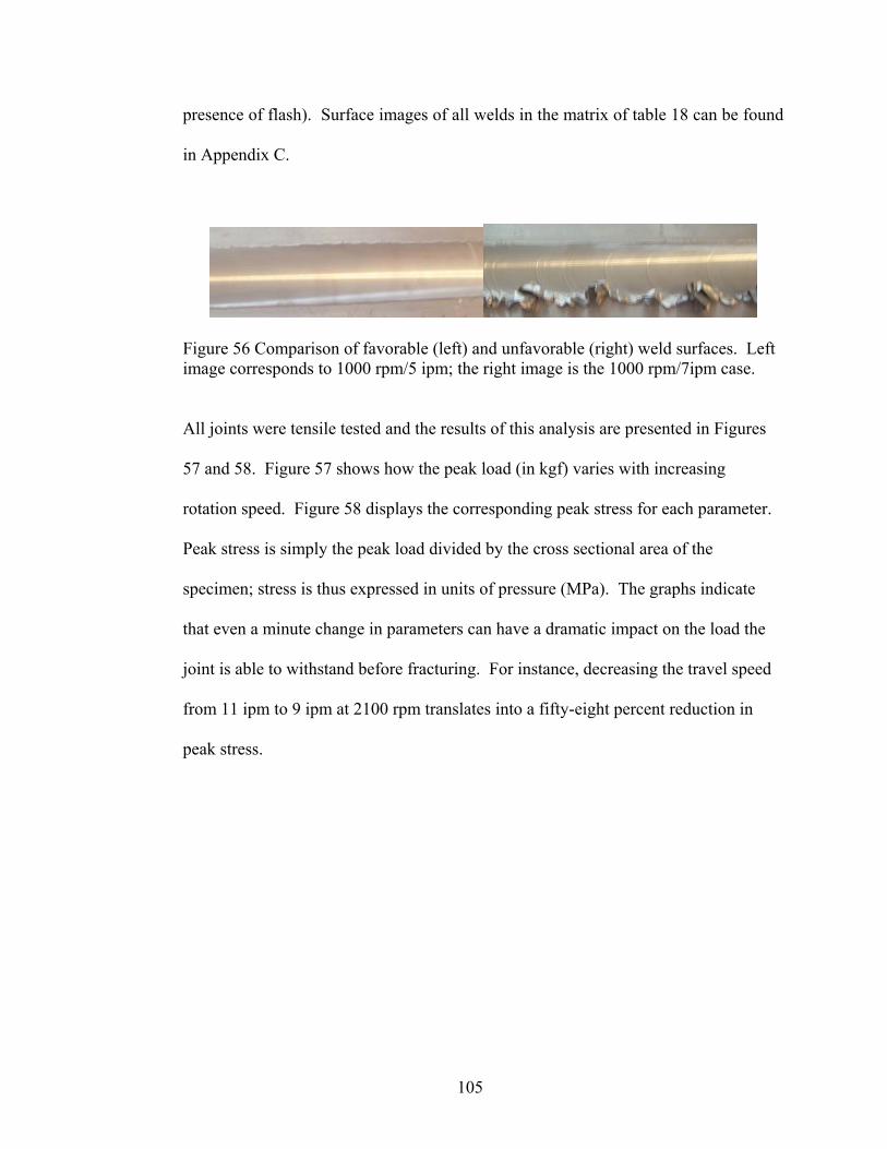
presence of flash). Surface images of all welds in the matrix of table 18 can be found
in Appendix C.
Figure 56 Comparison of favorable (left) and unfavorable (right) weld surfaces. Left image corresponds to 1000 rpm/5 ipm; the right image is the 1000 rpm/7ipm case.
All joints were tensile tested and the results of this analysis are presented in Figures
57 and 58. Figure 57 shows how the peak load (in kgf) varies with increasing
rotation speed. Figure 58 displays the corresponding peak stress for each parameter.
Peak stress is simply the peak load divided by the cross sectional area of the
specimen; stress is thus expressed in units of pressure (MPa). The graphs indicate
that even a minute change in parameters can have a dramatic impact on the load the
joint is able to withstand before fracturing. For instance, decreasing the travel speed
from 11 ipm to 9 ipm at 2100 rpm translates into a fifty-eight percent reduction in
peak stress.
105
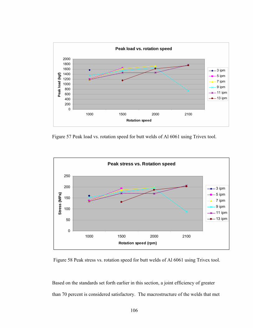
Peak load vs. rotation speed
0200400600800
100012001400160018002000
1000 1500 2000 2100
Rotation speed
Pea
k lo
ad (k
gf) 3 ipm
5 ipm7 ipm9 ipm11 ipm13 ipm
Figure 57 Peak load vs. rotation speed for butt welds of Al 6061 using Trivex tool.
Peak stress vs. Rotation speed
0
50
100
150
200
250
1000 1500 2000 2100
Rotation speed (rpm)
Stre
ss (M
Pa)
3 ipm5 ipm7 ipm9 ipm11 ipm13 ipm
Figure 58 Peak stress vs. rotation speed for butt welds of Al 6061 using Trivex tool.
Based on the standards set forth earlier in this section, a joint efficiency of greater
than 70 percent is considered satisfactory. The macrostructure of the welds that met
106

this condition were analyzed. Those with defects were subsequently eliminated; the
remaining welds comprise the operating window charted in Table 18. Microscopic
images of the macrographs for the acceptable welds are shown in Figure 59.
a) 1500 rpm, 5 ipm
b) 1500 rpm, 7 ipm
c) 2000 rpm, 7 ipm
107
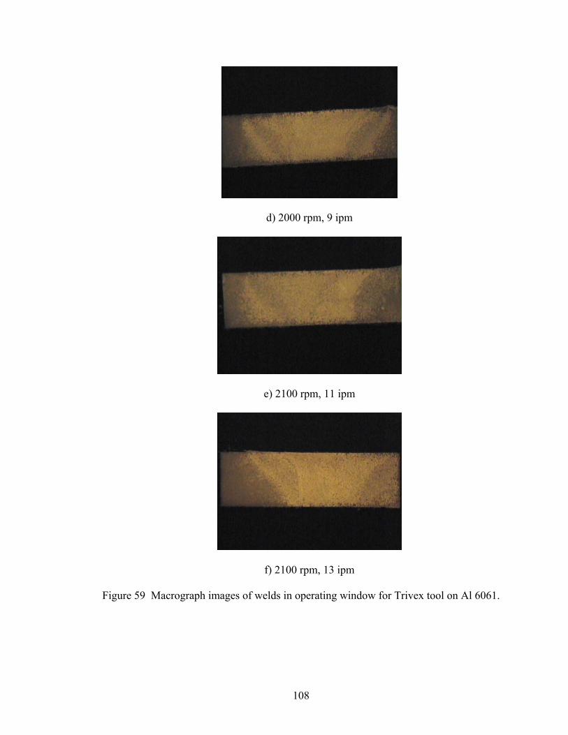
d) 2000 rpm, 9 ipm
e) 2100 rpm, 11 ipm
f) 2100 rpm, 13 ipm
Figure 59 Macrograph images of welds in operating window for Trivex tool on Al 6061.
108
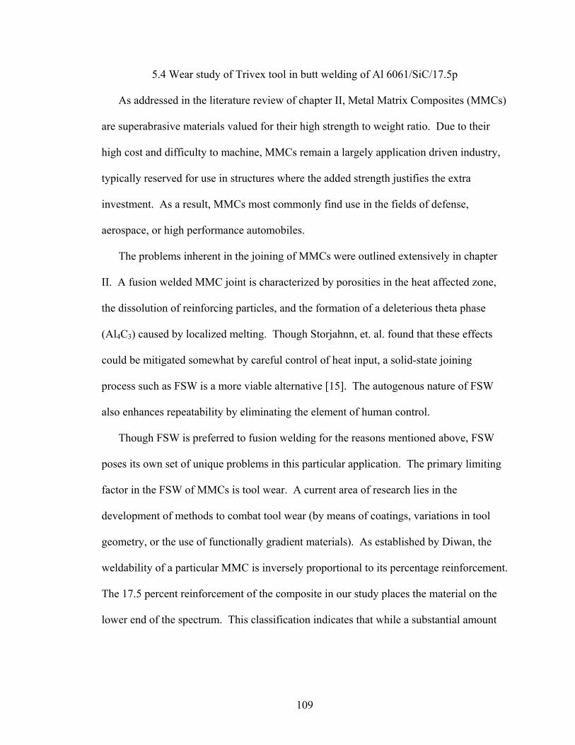
5.4 Wear study of Trivex tool in butt welding of Al 6061/SiC/17.5p
As addressed in the literature review of chapter II, Metal Matrix Composites (MMCs)
are superabrasive materials valued for their high strength to weight ratio. Due to their
high cost and difficulty to machine, MMCs remain a largely application driven industry,
typically reserved for use in structures where the added strength justifies the extra
investment. As a result, MMCs most commonly find use in the fields of defense,
aerospace, or high performance automobiles.
The problems inherent in the joining of MMCs were outlined extensively in chapter
II. A fusion welded MMC joint is characterized by porosities in the heat affected zone,
the dissolution of reinforcing particles, and the formation of a deleterious theta phase
(Al4C3) caused by localized melting. Though Storjahnn, et. al. found that these effects
could be mitigated somewhat by careful control of heat input, a solid-state joining
process such as FSW is a more viable alternative [15]. The autogenous nature of FSW
also enhances repeatability by eliminating the element of human control.
Though FSW is preferred to fusion welding for the reasons mentioned above, FSW
poses its own set of unique problems in this particular application. The primary limiting
factor in the FSW of MMCs is tool wear. A current area of research lies in the
development of methods to combat tool wear (by means of coatings, variations in tool
geometry, or the use of functionally gradient materials). As established by Diwan, the
weldability of a particular MMC is inversely proportional to its percentage reinforcement.
The 17.5 percent reinforcement of the composite in our study places the material on the
lower end of the spectrum. This classification indicates that while a substantial amount
109
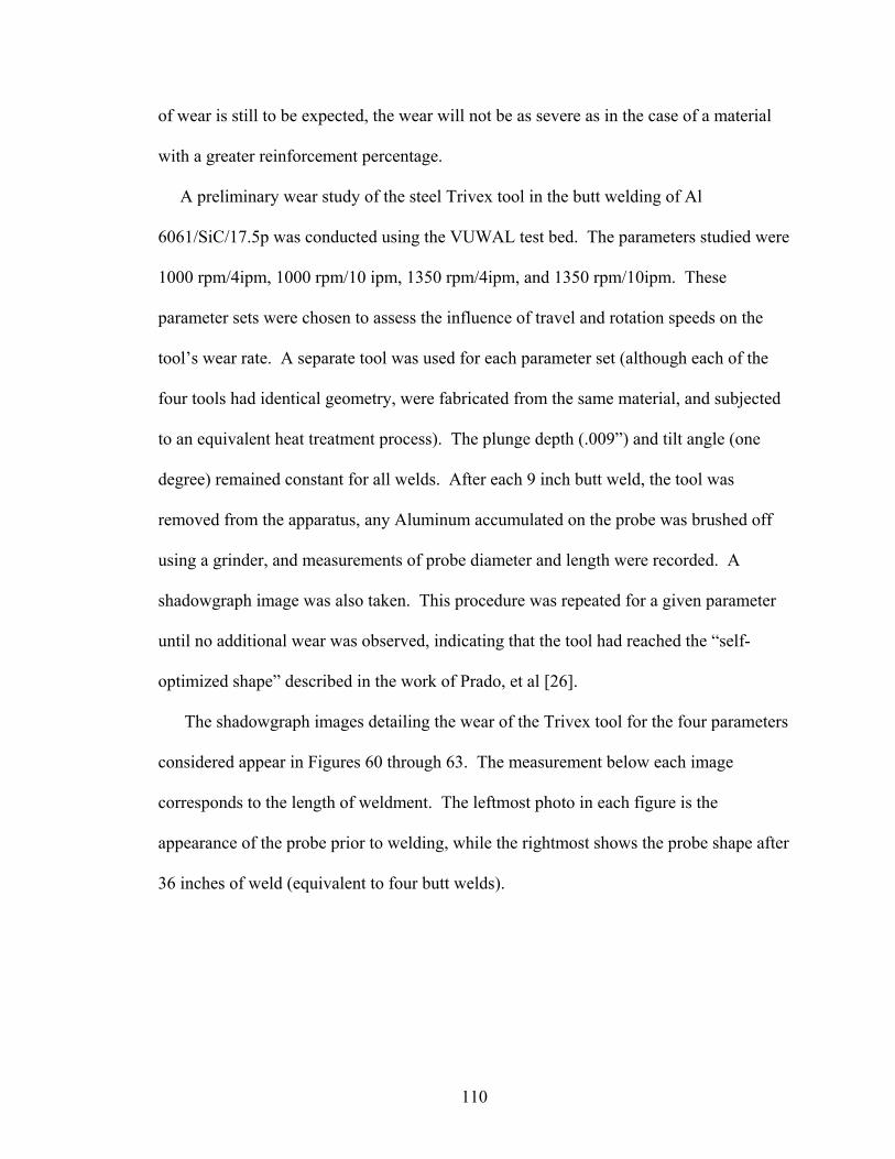
of wear is still to be expected, the wear will not be as severe as in the case of a material
with a greater reinforcement percentage.
A preliminary wear study of the steel Trivex tool in the butt welding of Al
6061/SiC/17.5p was conducted using the VUWAL test bed. The parameters studied were
1000 rpm/4ipm, 1000 rpm/10 ipm, 1350 rpm/4ipm, and 1350 rpm/10ipm. These
parameter sets were chosen to assess the influence of travel and rotation speeds on the
tool’s wear rate. A separate tool was used for each parameter set (although each of the
four tools had identical geometry, were fabricated from the same material, and subjected
to an equivalent heat treatment process). The plunge depth (.009”) and tilt angle (one
degree) remained constant for all welds. After each 9 inch butt weld, the tool was
removed from the apparatus, any Aluminum accumulated on the probe was brushed off
using a grinder, and measurements of probe diameter and length were recorded. A
shadowgraph image was also taken. This procedure was repeated for a given parameter
until no additional wear was observed, indicating that the tool had reached the “self-
optimized shape” described in the work of Prado, et al [26].
The shadowgraph images detailing the wear of the Trivex tool for the four parameters
considered appear in Figures 60 through 63. The measurement below each image
corresponds to the length of weldment. The leftmost photo in each figure is the
appearance of the probe prior to welding, while the rightmost shows the probe shape after
36 inches of weld (equivalent to four butt welds).
110
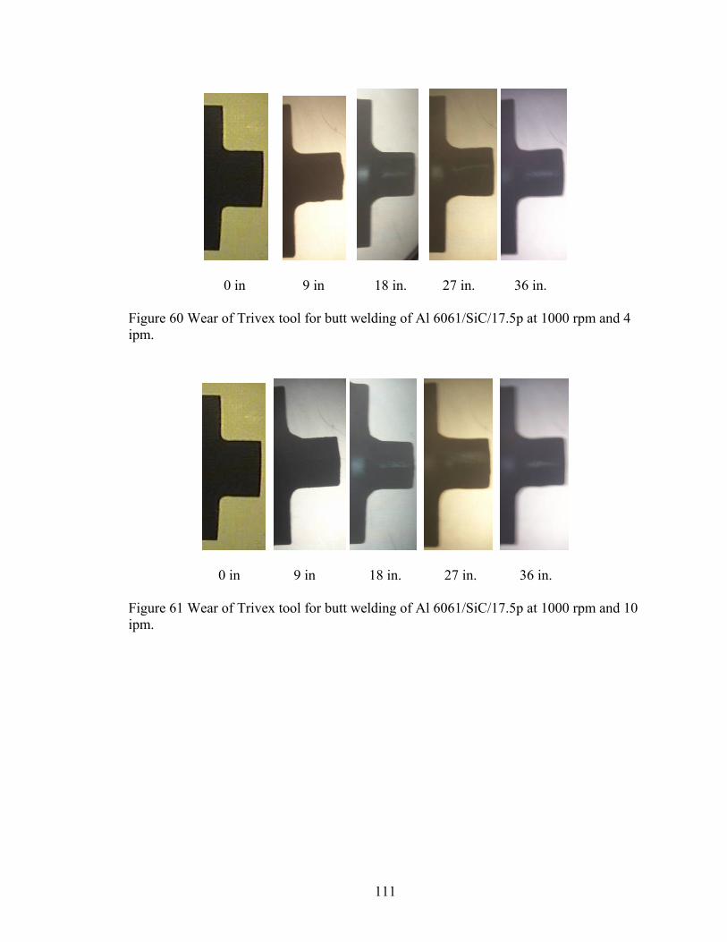
0 in 9 in 18 in. 27 in. 36 in.
Figure 60 Wear of Trivex tool for butt welding of Al 6061/SiC/17.5p at 1000 rpm and 4 ipm.
0 in 9 in 18 in. 27 in. 36 in.
Figure 61 Wear of Trivex tool for butt welding of Al 6061/SiC/17.5p at 1000 rpm and 10 pm. i
111
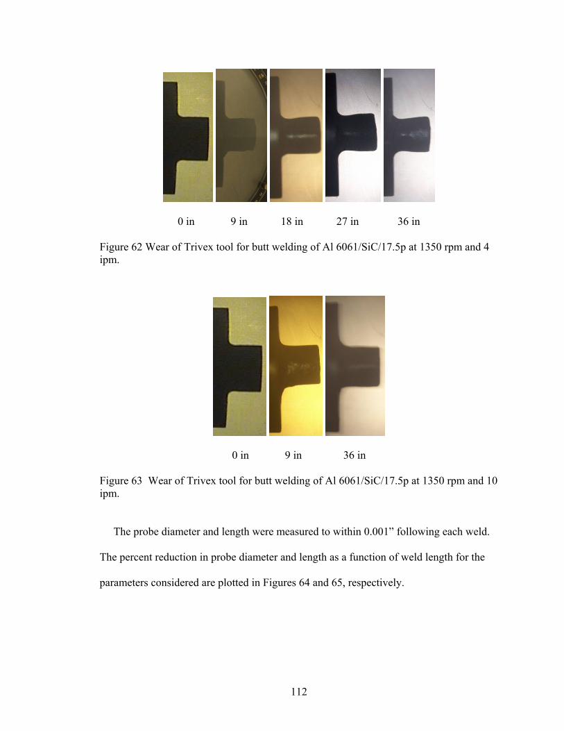
0 in 9 in 18 in 27 in 36 in
Figure 62 Wear of Trivex tool for butt welding of Al 6061/SiC/17.5p at 1350 rpm and 4 ipm.
0 in 9 in 36 in
Figure 63 Wear of Trivex tool for butt welding of Al 6061/SiC/17.5p at 1350 rpm and 10 m. ip
The probe diameter and length were measured to within 0.001” following each weld.
The percent reduction in probe diameter and length as a function of weld length for the
parameters considered are plotted in Figures 64 and 65, respectively.
112
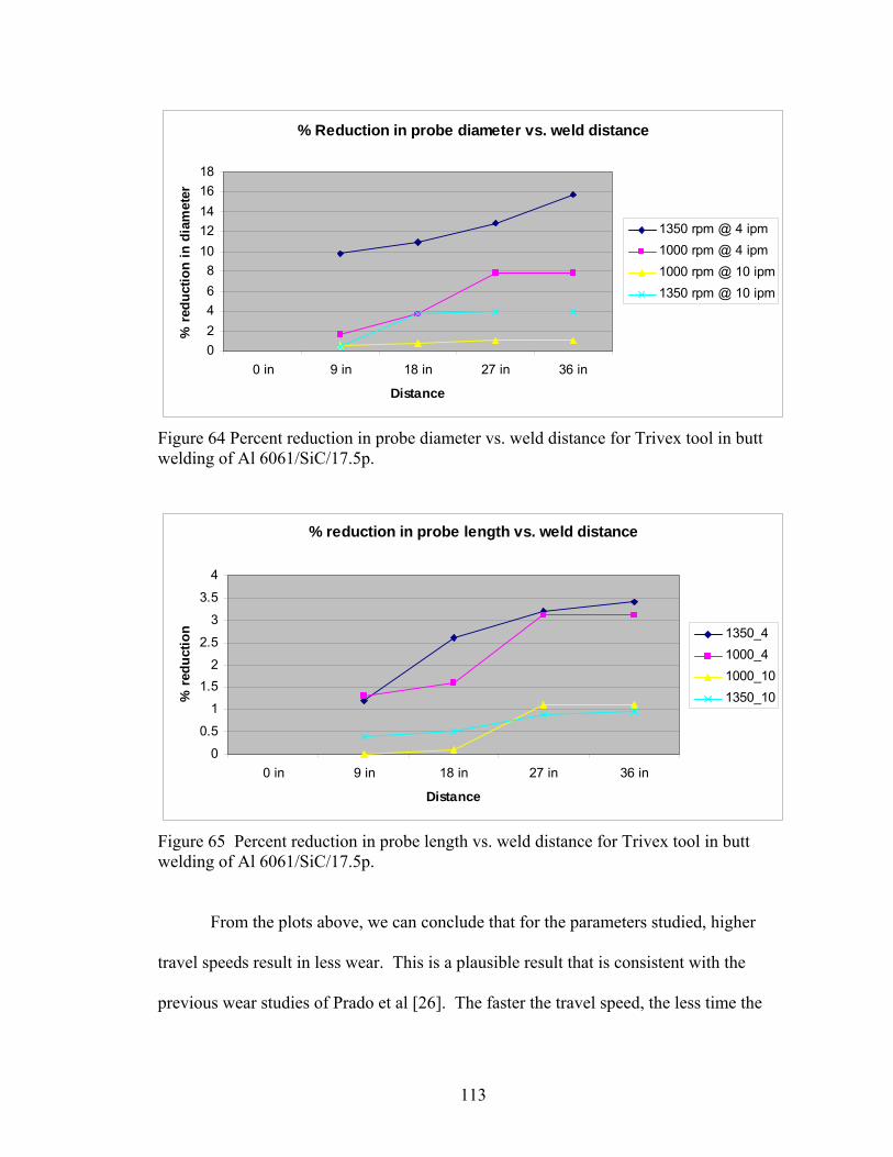
igure 64 Percent reduction in probe diameter vs. weld distance for Trivex tool in butt elding of Al 6061/SiC/17.5p.
igure 65 Percent reduction in probe length vs. weld distance for Trivex tool in butt welding of Al 6061/SiC/17.5p.
% Reduction in probe diameter vs. weld distance
02468
1012141618
0 in 9 in 18 in 27 in 36 in
% r
educ
tion
in d
iam
eter
1350 rpm @ 4 ipm 1000 rpm @ 4 ipm1000 rpm @ 10 ipm 1350 rpm @ 10 ipm
Distance
Fw
% reduction in probe length vs. weld distance
0
0.5
1
1.52
2.5
3
3.5
4
0 in 9 in 18 in 27 in 36 in
% r
educ
tion
1350_4 1000_41000_10 1350_10
Distance
F
From the plots above, we can conclude that for the parameters studied, higher
travel speeds result in less wear. This is a plausible result that is consistent with the
previous wear studies of Prado et al [26]. The faster the travel speed, the less time the
113
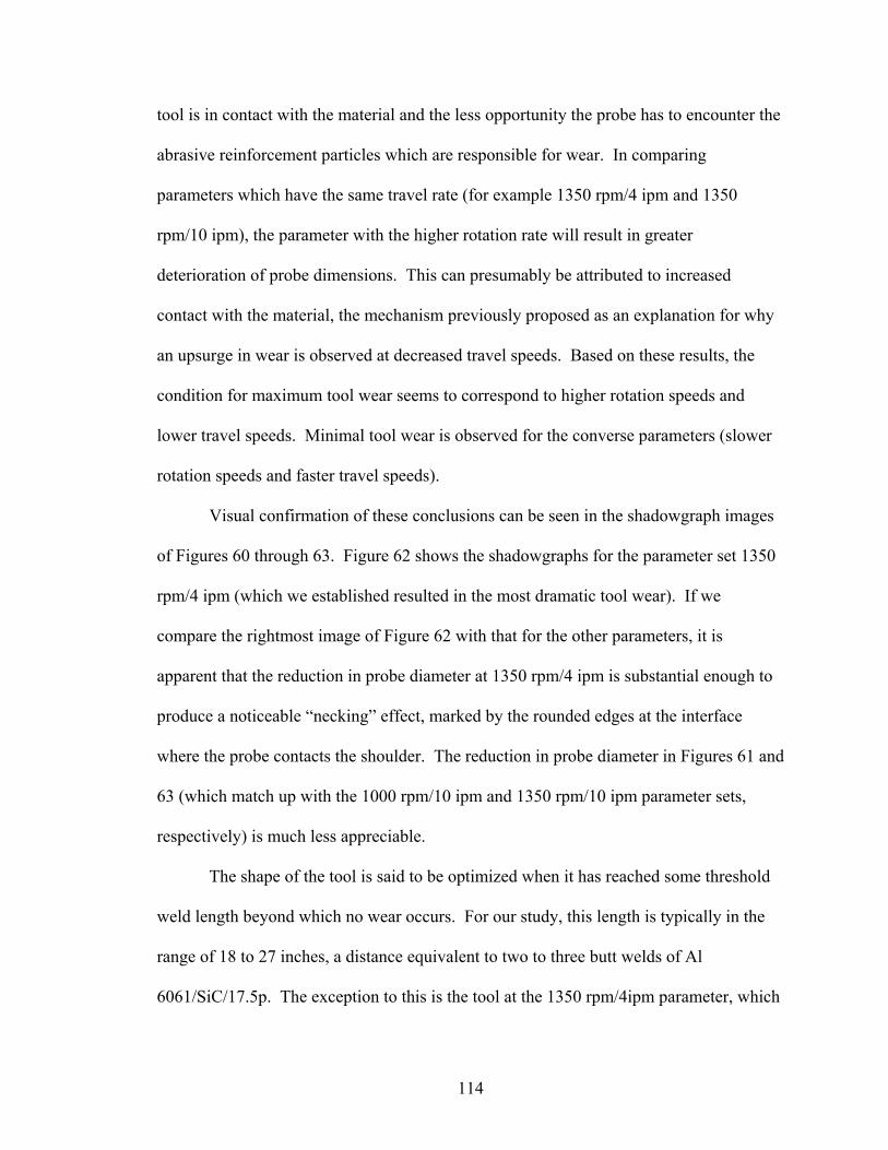
tool is in contact with the material and the less opportunity the probe has to enco
abrasive reinforcement particles which are responsible for wear. In comparing
parameters which have the same travel rate (for example 1350 rpm/4 ipm and
rpm/10 ipm), the parameter with the higher rotation rate will result in greater
deterioration of probe dimensions. This can presumably be attributed to increased
contact with the material, the mechanism previously proposed as an explanation for wh
an upsurge in wear is observed at decreased travel speeds. Based on these results, the
condition for maximum tool wear seems to correspond to higher rotation speeds and
lower travel speeds. Minimal tool wear is o
unter the
1350
y
bserved for the converse parameters (slower
t 1350
to
and
10 ipm and 1350 rpm/10 ipm parameter sets,
y in the
ch
rotation speeds and faster travel speeds).
Visual confirmation of these conclusions can be seen in the shadowgraph images
of Figures 60 through 63. Figure 62 shows the shadowgraphs for the parameter se
rpm/4 ipm (which we established resulted in the most dramatic tool wear). If we
compare the rightmost image of Figure 62 with that for the other parameters, it is
apparent that the reduction in probe diameter at 1350 rpm/4 ipm is substantial enough
produce a noticeable “necking” effect, marked by the rounded edges at the interface
where the probe contacts the shoulder. The reduction in probe diameter in Figures 61
63 (which match up with the 1000 rpm/
respectively) is much less appreciable.
The shape of the tool is said to be optimized when it has reached some threshold
weld length beyond which no wear occurs. For our study, this length is typicall
range of 18 to 27 inches, a distance equivalent to two to three butt welds of Al
6061/SiC/17.5p. The exception to this is the tool at the 1350 rpm/4ipm parameter, whi
114
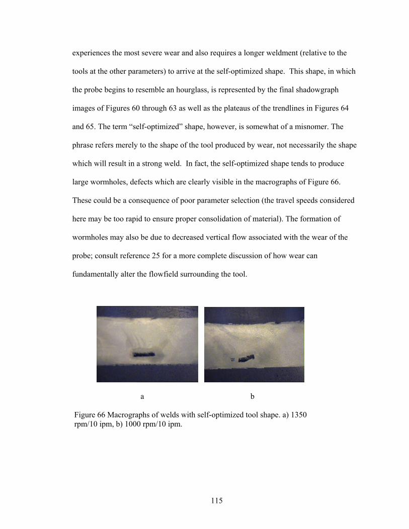
experiences the most severe wear and also requires a longer weldment (relative to the
tools at the other parameters) to arrive at the self-optimized shape. This shape, in wh
the probe begins to resemble an hourglass, is represented by the final shadowgraph
images of Figures 60 through 63 as well as the plateaus of the trendlines in Figures 64
and 65. The term “self-optimized” shape, however, is somewhat of a misnomer. The
phrase refers merely to the shape of the tool produced by wear, not necessarily the sha
which will result in a strong weld. In fact, the self-optimized shape tends to produce
large wormholes, defects which are clearly visible in the macrographs of Figure 66.
These could be a consequence of poor parameter selection (the travel speeds conside
here may be too rapid to ensure proper consolidation of material). The formation of
wormholes may also be due to decreased vertical flow associated with the we
probe; consult reference 25 for a more complete discuss
ich
pe
red
ar of the
ion of how wear can
ndamentally alter the flowfield surrounding the tool.
Figure 66 Macrographs of welds with self-optimized tool shape. a) 1350 rpm/10 ipm, b) 1000 rpm/10 ipm.
fu
a b
115
There are some shortcomings to our research methodology that should be noted.
In the case of the Trivex tool, methods which rely on optical comparators as a qualitative
measurement of tool wear present some limitations. The shadowgraph generates only a
two-dimensional image and hence is not able to accurately capture the Trivex geomet
This is evident in the “before” images of Figures 60 through 63, in which the Trivex
probe appears in profile as a smooth cylinder. Another problem with the shadowgrap
method is its inability to reflect the often asymmetric manner in which wear occurs.
During the course of the study, an effort was made to take each shadowgraph image from
the same angle and at the same magnification. Thus while the shadowgraph images ar
effective at conveying the wear on one fa
ry.
h
e
ce of the tool, they reveal nothing about the
he
n
n
the
progression of wear at other locations.
The dimensions of the tool were measured periodically using a digital
micrometer; this data serves as the basis for the plots in Figures 64 and 65. Because t
tool wears asymmetrically, measurements are location dependent. That is, the probe
length at one point on the tool may or may not be equal to the length measured at another
point. The non-cylindrical Trivex geometry makes it difficult to obtain a representative
value for the probe diameter. The values used in the calculation of diameter and probe
reduction were typically an average of three measurements taken at various locations o
the tool. Additionally, our measurements do not account for wear of the shoulder. If
shoulder wear occurs, it would translate into a consistent underestimation of the reductio
in probe length. Severe shoulder wear could even produce data that would indicate
probe is becoming longer with successive welds (a nonsensical result). For future
116
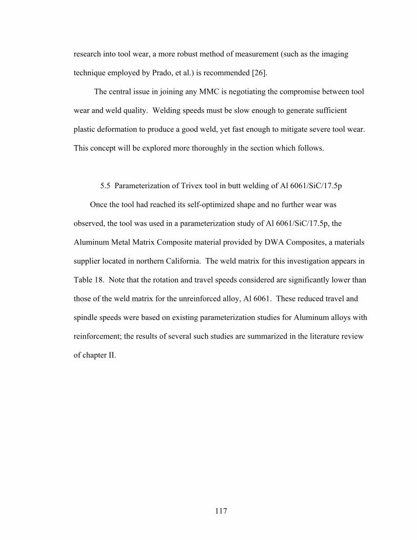
research into tool wear, a more robust method of measurement (such as the imaging
technique employed by Prado, et al.) is recommended [26].
The central issue in joining any MMC is negotiating the compromise between tool
wear and weld quality. Welding speeds must be slow enough to generate sufficient
lastic deformation to produce a good weld, yet fast enough to mitigate severe tool wear.
This co
ere based on existing parameterization studies for Aluminum alloys with
inforcement; the results of several such studies are summarized in the literature review
f chapter II.
p
ncept will be explored more thoroughly in the section which follows.
5.5 Parameterization of Trivex tool in butt welding of Al 6061/SiC/17.5p
Once the tool had reached its self-optimized shape and no further wear was
observed, the tool was used in a parameterization study of Al 6061/SiC/17.5p, the
Aluminum Metal Matrix Composite material provided by DWA Composites, a materials
supplier located in northern California. The weld matrix for this investigation appears in
Table 18. Note that the rotation and travel speeds considered are significantly lower than
those of the weld matrix for the unreinforced alloy, Al 6061. These reduced travel and
spindle speeds w
re
o
117
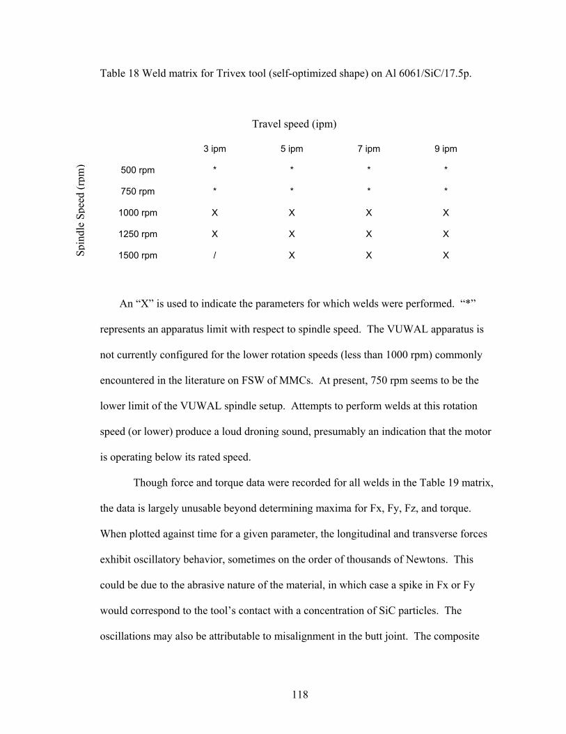
Table 18 Weld matrix for Trivex tool (self-optimized shape) on Al 6061/SiC/17.5p.
3 ipm 5 ipm 7 ipm 9 ipm
X X X
X X X
p. Attempts to perform welds at this rotation
s
is
ite
500 rpm * * * *
750 rpm * * * *
1000 rpm X
1250 rpm X
1500 rpm / X X X
An “X” is used to indicate the parameters for which welds were performed. “*”
represents an apparatus limit with respect to spindle speed. The VUWAL apparatus is
not currently configured for the lower rotation speeds (less than 1000 rpm) commonly
encountered in the literature on FSW of MMCs. At present, 750 rpm seems to be the
lower limit of the VUWAL spindle setu
Travel s ed (ipm)
S
pe
speed (or lower) produce a loud droning sound, presumably an indication that the motor
is operating below its rated speed.
Though force and torque data were recorded for all welds in the Table 19 matrix,
the data is largely unusable beyond determining maxima for Fx, Fy, Fz, and torque.
When plotted against time for a given parameter, the longitudinal and transverse force
exhibit oscillatory behavior, sometimes on the order of thousands of Newtons. Th
could be due to the abrasive nature of the material, in which case a spike in Fx or Fy
would correspond to the tool’s contact with a concentration of SiC particles. The
oscillations may also be attributable to misalignment in the butt joint. The compos
pind
le S
peed
(rpm
)
118
material is initially in 84” long x 12” wide x ¼” thick sheets which are cut into the 9”
long x 3” wide x ¼” thick strips used for butt welds. The extreme stiffness of the
material makes it incredibly difficult to machine; consequently the cuts are often uneven
When selecting two strips to join, it is not always possible to
.
ensure either a perfect fit or
or
a for the MMC welds will be presented more completely in chapter VI, where
han
unt for the
difference in as-welded surface consistency between the materials. The typical surface
structure of a Al 6061/SiC/17.5p butt joint is pictured in Figure 67.
a straight joint line. Thus, gapping and/or variation along the path of the joint line may
be responsible for the inconsistencies in the x and y forces.
Additionally, it is difficult to determine average values for steady state axial force
and torque at the slower travel speeds (three inches per minute) considered. In this
instance, the “creep” (the reduced speed at which the tool enters the material to generate
sufficient heat for plasticization) is only slightly less than the actual weld speed. The
“ramp” on the force graph which indicates the transition between the “creep” phase and
the weld is thus absent, making it difficult to distinguish which values comprise the
steady state condition. With these caveats stated, the average force and torque values f
butt welds of the Trivex (self-optimized shape) on Al 6061/SiC/17.5p do not display the
consistent trends associated with butt welds of the tool on Al 6061 (section 5.4). The
force dat
they will serve as the inputs for a finite element model to predict tool deformation and
stress.
The surfaces of the butt welds of Al 6061/SiC/17.5p have a rougher texture t
those of Al 6061 discussed in the previous section. The composite material is coarser in
the pre-welded state than its unreinforced counterpart, which may acco
119
Figure 67 Welded surface of Al 6061/SiC/17.5p. Performed at 1250 rpm, 3 ipm using Trivex tool with self-optimized shape.
The abrasive nature of Al 6061/SiC/17.5p precludes tensile testing as a quantitative
measure of joint efficiency. Characteristic sections of the welds were cut using a
diamond saw, but were unable to be milled into the tensile test samples sketched in
Figure 28 using conventional machining methods. Waterjet cutting or electron discharge
the
term synonymous with operating window) is
y the blue shaded region of Table 19. The accompanying macrographs
machining (EDM) are possible options for any future research which may require an
assessment of joint strength.
Since no tensile data was collected, it was necessary to cross-section all welds in
the matrix of table 18 using the method outlined in chapter III. Since the shape of the
self-optimized Trivex tool is effectively the same as that of a smooth probe, it is expected
that a majority of the welds will exhibit wormhole defects. The operating window for
butt welding of Al 6061/SiC/17.5p is thus comprised of those welds that were deemed
“defect-free.” The weld envelope (a
designated b
appear in Figure 68.
120
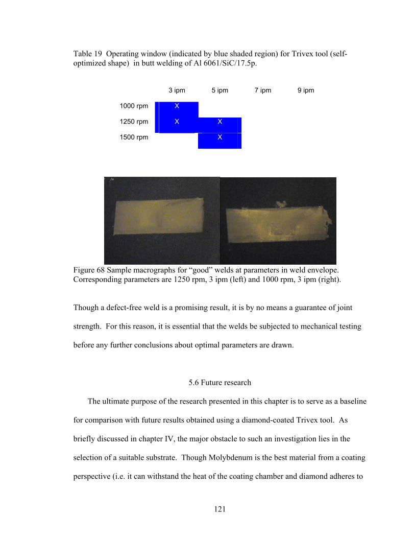
Table 19 Operatin window ated by haded ) for T ool (self-optimized shape) in butt welding of Al 6061/SiC/17.5p.
3 ipm 5 ipm 7 ipm 9 ipm
1000 rpm
g (indic blue s region rivex t
X
1250 rpm X X
1500 rpm X
Figure 68 Sample macrographs for “good” welds at parameters in weld envelope.
Though a defect-free weld is a promising result, it is by no means a g
Corresponding parameters are 1250 rpm, 3 ipm (left) and 1000 rpm, 3 ipm (right).
uarantee of joint
trength. For this reason, it is essential that the welds be subjected to mechanical testing
before any further conclusions abo are drawn.
line
ting
s
ut optimal parameters
5.6 Future research
The ultimate purpose of the research presented in this chapter is to serve as a base
for comparison with future results obtained using a diamond-coated Trivex tool. As
briefly discussed in chapter IV, the major obstacle to such an investigation lies in the
selection of a suitable substrate. Though Molybdenum is the best material from a coa
perspective (i.e. it can withstand the heat of the coating chamber and diamond adheres to
121
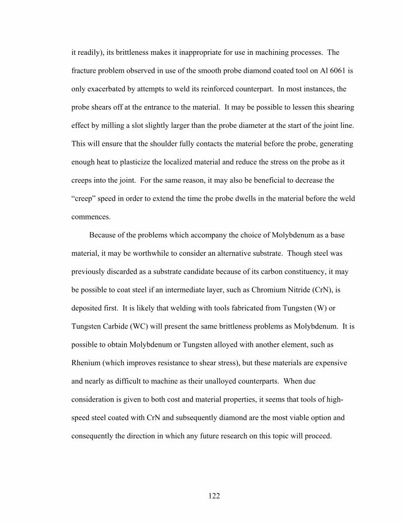
it readily), its brittleness makes it inappropriate for use in machining processes. The
fracture problem observed in use of the smooth probe diamond coated tool on Al 6061 is
only exacerbated by attempts to weld its reinforced counterpart. In most instances, the
probe shears off at the entrance to the material. It may be possible to lessen this shearing
effect by milling a slot slightly larger than the probe diameter at the start of the joint lin
This will ensure that the shoulder fully contacts the material before the probe, gener
enough heat to plasticize the localized material and reduce the stress on the probe as it
creeps into th
e.
ating
e joint. For the same reason, it may also be beneficial to decrease the
ld
ay
s
h as
-
“creep” speed in order to extend the time the probe dwells in the material before the we
commences.
Because of the problems which accompany the choice of Molybdenum as a base
material, it may be worthwhile to consider an alternative substrate. Though steel was
previously discarded as a substrate candidate because of its carbon constituency, it m
be possible to coat steel if an intermediate layer, such as Chromium Nitride (CrN), is
deposited first. It is likely that welding with tools fabricated from Tungsten (W) or
Tungsten Carbide (WC) will present the same brittleness problems as Molybdenum. It i
possible to obtain Molybdenum or Tungsten alloyed with another element, suc
Rhenium (which improves resistance to shear stress), but these materials are expensive
and nearly as difficult to machine as their unalloyed counterparts. When due
consideration is given to both cost and material properties, it seems that tools of high
speed steel coated with CrN and subsequently diamond are the most viable option and
consequently the direction in which any future research on this topic will proceed.
122
The potential outcomes for the use of a coated tool are promising. The results of
chapter IV demonstrate that a coated tool can significantly reduce the values of force an
torque in the welding of Al 6061. It may be that a similar force reduction will be
observed when the coated tool is applied to Al 6061/SiC/17.5p. Additionally, it is hope
that the coated tool will exhibit decreased wear. Though tool wear is little more than a
peripheral concer
d
d
n in the joining of Aluminum alloys, it is the limiting factor in the
lding of Metal Matrix Composites. As such, any innovation which can be shown to
duce the wear rate of tools in these materials would be of considerable benefit to the
dustry.
we
re
in
123
CHAPTER VI
D ON FORCE DATA
ined.
r
o
st
ructive. The model
presented here is a three-dimensional static model in which forces obtained from the
dynamo houlder in order to produce a “snapshot” of
tool deformation and
FINITE ELEMENT MODEL OF TOOL DEFORMATION AND STRESS BASE
The focus of this chapter is to construct and implement a finite element model of tool
deformation and stress during the Friction Stir Welding process. By emphasizing the
modeling aspect of FSW research, we do not wish to discount the value of experimental
work presented in chapters IV and V. Much can be learned about a process by physically
varying the parameters and analyzing the effect these changes have on the data obta
There is, however, error (be it human or otherwise) that is inherent in any experimental
procedure. This is not to say that modeling eliminates error; is it relatively common fo
models to generate outcomes which do not fully agree with those obtained through
experimentation. This divergence from experimental results can usually be attributed t
assumptions made during the model’s development stages. A simple FEA method to
model deformation and/or stress is perhaps most advantageous from an industry co
standpoint in that it would enable researchers to predict the wear behavior for a given
tool/workpiece material combination while minimizing experimentation that is both time
consuming and, in the case of Metal Matrix Composites, dest
meter are applied to the probe and s
stress for various welding parameters.
124
6.1 An Overview of the Finite Element Method
Finite element analysis (FEA) is a numerical method developed to analyze
engineering problems for which a closed form solution does not exist. The method
involves dividing a body into discrete elements connected by nodes. The behavior at
each node can then be analyzed. In this manner, FEA can be used to characterize the
behavior of the structure as a whole. The major advantages of FEA are the ability to
model ifferent materials,
han
would
1)
or temperatures are expected to be changing
irregularly shaped bodies as well as those comprised of several d
dle any number and type of boundary conditions, and save time and money that
be required for large-scale experimentation on a structure [34].
There are essentially eight steps in any finite element analysis:
In discretization, the body is divided into elements linked by nodes. For a two-
dimensional analysis, common elements include multi-noded line elements (used
to represent bars or beams), triangular, and quadrilateral elements. Three-
dimensional elements include tetrahedrals, hexahedrals, wedges, etc. and may be
regular or irregularly shaped depending upon the geometry of the structure being
modeled. The choice and number of elements depends on the nature of the
structure under consideration as well as the level of accuracy desired. It is
common engineering practice to use more elements with smaller dimensions in
areas where stresses, displacements,
or at a maximum (locations where a high level of accuracy is desired). Fewer
elements with larger dimensions are appropriate for regions where results are
expected to be largely unchanging.
125
Together, the elements and nodes of a structure comprise what is referred to as the
mesh. The usability of a finite element analysis hinges largely on the choice of
elements and the level of mesh refinement. To assess mesh refinement, a
sequence of analyses is conducted in which the number of elements is
successively increased (or decreased). When the results of the analyses converge,
the mesh is said to be sufficiently refined. It should be noted that refinement is
not an indicator of the accuracy of the model, but a check performed as a way to
y
al
z for the three-dimensional case). Depending on the type of
4)
minimize computational time. For instance, we may be able to reduce the number
of tetrahedral elements in a structure from 2500 to 1500 without appreciabl
altering the results. This issue is of particular importance when using a finite
element computer package.
2) A nodal function is selected which expresses displacement in terms of the nod
variables (x, y, and
element, a linear, quadratic, cubic, quartic, or even trigonometric function may be
chosen [35]. The same displacement function is applied to each element,
thus utilizing discrete methods to characterize a quantity which is ultimately
continuous.
3) A relationship relating strain to displacement and stress to strain is now defined.
In the simplest case, strain in the x-direction as a function of displacement is
written as εx = du/dx. Stress and strain are then related by Hooke’s law, σx = E εx,
where E denotes Young’s modulus of elasticity.
The stiffness matrix, k, is derived using the direct equilibrium method,
work/energy methods, or Galerkin’s method (weighted residuals). For one-
126
dimensional elements, the direct equilibrium method is easily applied. Existing
relationships between local forces and deformations are exploited to express nodal
forces as a product of nodal displacements and k. Work/energy methods that can
be used to derive the stiffness matrix include minimum potential energy, the
before it is possible to solve the system.
sents an n x n square
tes an n x m column
matrix.
principle of virtual work, and Castigliano’s method. Galerkin’s method relies
primarily on the use of weighting functions. For further details on deriving an
element stiffness matrix using the methods briefly outlined above, the reader
should consult reference [34].
5) The equations generated in the above step are assembled into a global stiffness
matrix, K, which relates global forces to global displacements. Because K is
always a singular matrix, we must impose appropriate boundary conditions on the
structure
6) The system of equations given by {F} = [K] {d} is solved using a method from
linear algebra. Note that a quantity in square brackets repre
matrix, while a quantity surrounded by curved brackets deno
7) The values for displacements can then be used to calculate strain and
subsequently stress using the relationships defined in step 3.
8) The results of the finite element analysis are interpreted.
The steps outlined above are best suited for general loading conditions which are static in
nature. When dynamic effects are considered, a consistent mass matrix for each element
must be developed to account for time dependence. This matrix, [M], is specific to the
127
type of element and is derived using the principle of virtual work. For a complete
discussion of the consistent mass matrix, consult chapter 16 of reference [34]. The
governing equation in step (6) thus becomes {F(t)} = [K]{d} + [M]{d}. Hence, a finite
element solution for a dynamic system must include a procedure to calculate nodal
displacements, {d}, at incremental values of time (referred to in the FEA lexicon as time
steps). There are three p time steps: the central
diffe
analysis of the FSW tool. NASTRAN is the finite element solver which
eval sing
(con
PATRA is outlined
belo
1) from a CAD program.
ese can be selected
4)
location of forces and/or pressures applied to the body are specified.
rimary methods of direct integration using
rence method, the Newmark-Beta method, and the Wilson-Theta method. The latter
two are sophisticated algorithims which are used in many commercial FEA codes.
6.2 NASTRAN as Finite Element Solver
The finite element software package NASTRAN was used to carry out a finite
element
uates the stiffness matrix and solves for displacements and stresses. Pre-proces
structing and meshing the geometry) and post-processing of results is done in
N. The steps of a typical finite element analysis using NASTRAN
w:
The geometry is either built in PATRAN or imported
2) The geometry is meshed. The element verification feature in PATRAN can be
used to provide a preliminary assessment of the quality of the mesh.
3) The material properties of the geometry are specified. Th
from an existing library or input directly by the user.
The boundary conditions for the geometry are indicated. The magnitude and
128
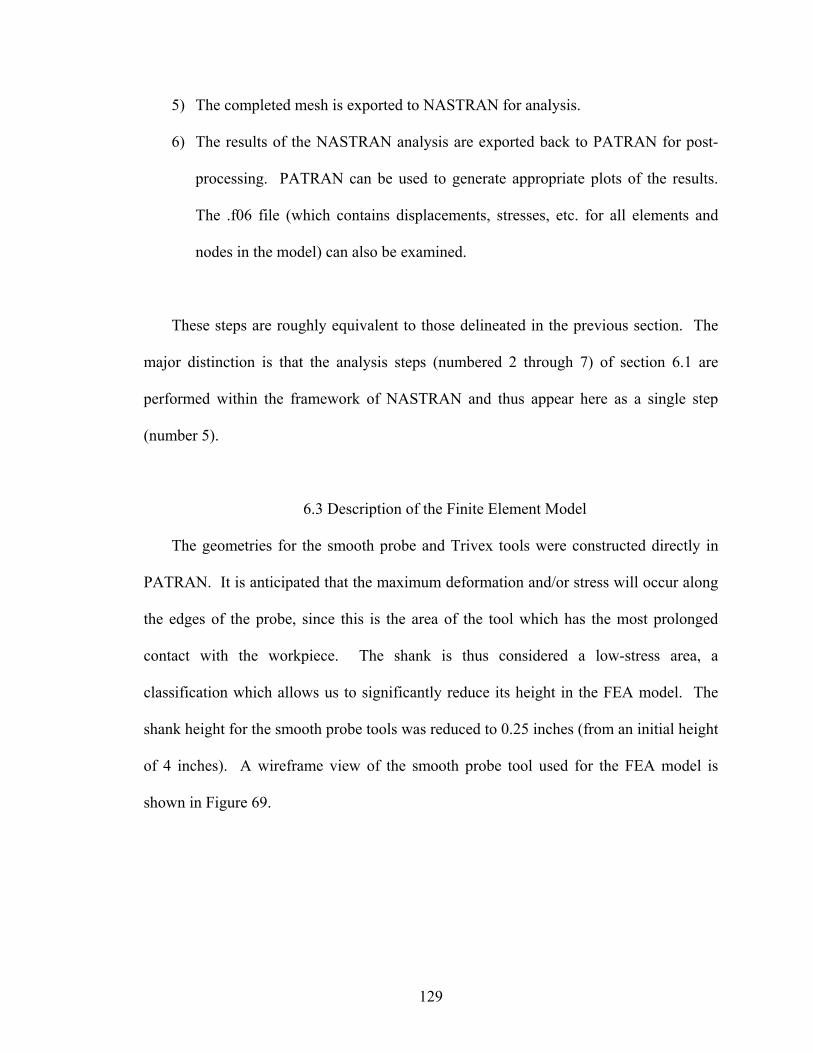
5)
6)
processing. PATRAN can be used to generate appropriate plots of the results.
e roughly equivalent to those delineated in the previous section. The
major distinction is that the analysis steps (numbered 2 through 7) of section 6.1 are
performed within the fr re as a single step
(num
lows us to significantly reduce its height in the FEA model. The
shank height for the smooth probe tools was reduced to 0.25 inches (from an initial height
of 4 inches). A wireframe view of the smooth probe tool used for the FEA model is
shown in Figure 69.
The completed mesh is exported to NASTRAN for analysis.
The results of the NASTRAN analysis are exported back to PATRAN for post-
The .f06 file (which contains displacements, stresses, etc. for all elements and
nodes in the model) can also be examined.
These steps ar
amework of NASTRAN and thus appear he
ber 5).
6.3 Description of the Finite Element Model
The geometries for the smooth probe and Trivex tools were constructed directly in
PATRAN. It is anticipated that the maximum deformation and/or stress will occur along
the edges of the probe, since this is the area of the tool which has the most prolonged
contact with the workpiece. The shank is thus considered a low-stress area, a
classification which al
129
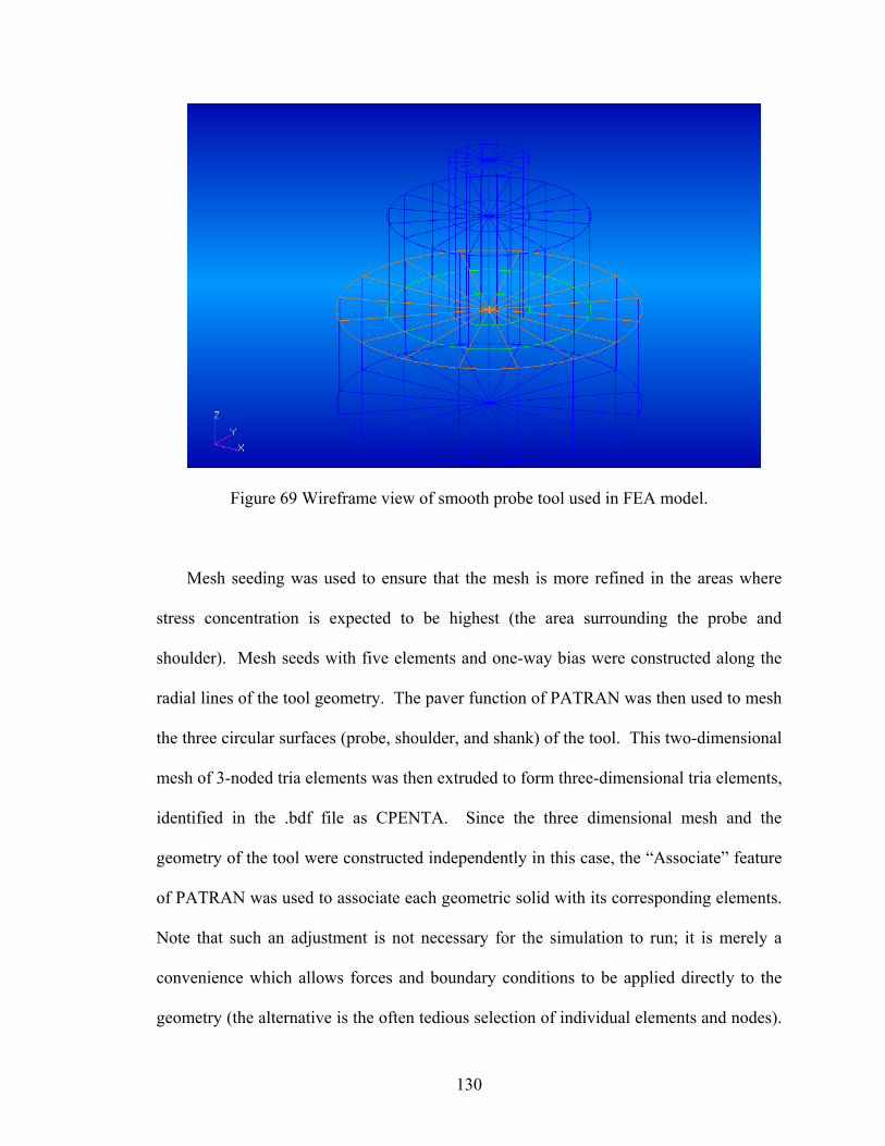
Figure 69 Wireframe view of smooth probe tool used in FEA model.
Mesh seeding was used to ensure that the mesh is more refined in the areas where
stress concentration is expected to be highest (the area surrounding the probe and
shoulder). Mesh seeds with five elements and one-way bias were constructed along the
radial lines of the tool geometry. The paver function of PATRAN was then used to mesh
the three circular surfaces (probe, shoulder, and shank) of the tool. This two-dimensional
mesh of 3-noded tria elements was then extruded to form three-dimensional tria elements,
identified in the .bdf file as CPENTA. Since the three dimensional mesh and the
geometry of the tool were constructed independently in this case, the “Associate” feature
of PATRAN was used to associate each geometric solid with its corresponding elements.
Note that such an adjustment is not necessary for the simulation to run; it is merely a
convenience which allows forces and boundary conditions to be applied directly to the
geometry (the alternative is the often tedious selection of individual elements and nodes).
130
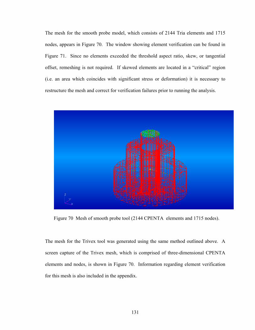
The mesh for the smooth probe model, which consists of 2144 Tria elements and 1715
nodes, appears in Figure 70. The window showing element verification can be found in
Figure 71. Since no elements exceeded the threshold aspect ratio, skew, or tangential
offset, remeshing is not required. If skewed elements are located in a “critical” region
(i.e. an area which coincides with significant stress or deformation) it is necessary to
restructure the mesh and correct for verification failures prior to running the analysis.
Figure 70 Mesh of smooth probe tool (2144 CPENTA elements and 1715 nodes).
The mesh for the Trivex tool was generated using the same method outlined above. A
screen capture of the Trivex mesh, which is comprised of three-dimensional CPENTA
elements and nodes, is shown in Figure 70. Information regarding element verification
for this mesh is also included in the appendix.
131
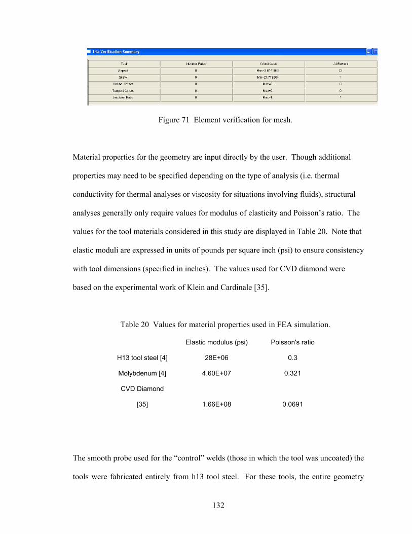
Figure 71 Element verification for mesh.
Material properties for the geometry are input directly by the user. Though additional
properties may need to be specified depending on the type of analysis (i.e. thermal
conductivity for thermal analyses or viscosity for situations involving fluids), structural
analyses generally only require values for modulus of elasticity and Poisson’s ratio. The
values for the tool materials considered in this study are displayed in Table 20. Note that
elastic moduli are expressed in units of pounds per square inch (psi) to ensure consistency
with tool dimensions (specified in inches). The values used for CVD diamond were
based on the experimental work of Klein and Cardinale [35].
Table 20 Values for material properties used in FEA simulation.
Elastic modulus (psi) Poisson's ratio
H13 tool steel [4] 28E+06 0.3
Molybdenum [4] 4.60E+07 0.321
CVD Diamond
[35] 1.66E+08 0.0691
The smooth probe used for the “control” welds (those in which the tool was uncoated) the
tools were fabricated entirely from h13 tool steel. For these tools, the entire geometry
132
could be assigned the properties of the base material. The prototype smooth probe tool,
however, consisted of a Molybdenum substrate coated with CVD diamond. The
properties associated with the diamond coating were specified for the surfaces of the
probe and shoulder (the regions on which the coating was deposited). The coating was
simulated using shell elements with thicknesses on the order of micrometers. The
location of these shell elements corresponded to the coated region. The remainder of the
geometry, including the ¼” long segment of the tool which represents the shank, was
given the properties of Molybdenum.
The variability of material properties with temperature should also be considered.
During the course of welding, we estimate that the tool’s temperature will increase from
room temperature (25 degrees Celsius) to the range of 400 to 600 C (depending on the
weld parameters). In the case of steel, this increase in temperature coincides with a
decrease in the modulus of elasticity (based on data from reference 4, this decrease may
be upwards of fifteen percent for the temperatures previously indicated).
Understandably, the variation of the modulus of CVD diamond with temperature is less
well-characterized. Since the objective of this study is to merely provide “ballpark”
estimates for tool deformation and stress based on force data, the effects of temperature
were largely ignored in the initial analysis.
The major obstacle barring the inclusion of temperature dependency in out model
is the nonuniformity of the temperature throughout the tool. The influence of geometry
and weld parameters on the temperature distribution is a subject of current modeling
research. Most investigations of this type use FLUENT, a computational fluid dynamics
program that is better suited for thermal analysis (because NASTRAN is a structural
133
analysis program, temperatures usually serve as inputs). Ideally, we could use FLUENT
to generate the temperature fields for a particular tool/workpiece/parameter combination
and then apply the results of this analysis to the structural model in NASTRAN. In this
way, the tool in the PATRAN pre-processor could be divided into geometric regions and
the material properties that correspond to the temperature in each region (based on the
results of the FLUENT simulation) could be specified. The caveat is that the results of
such FLUENT simulations must be experimentally verified, presumably using a thermal
camera or data acquired from thermocouples embedded in the workpiece. Though using
the output of FLUENT simulations as an input to NASTRAN could be a more accurate
way to model tool wear, it adds a level of complexity to our model that we are not yet
ready to manage.
To simulate the fastening of the tool into the collet, the underside of the tool is
constrained from translation and rotation in the x, y, and z directions. The tool geometry
with the appropriate boundary conditions applied is shown in Figure 72 for the smooth
probe. For a detailed description of which nodes the constraints were applied to, consult
the .bdf file in the Appendix D.
134
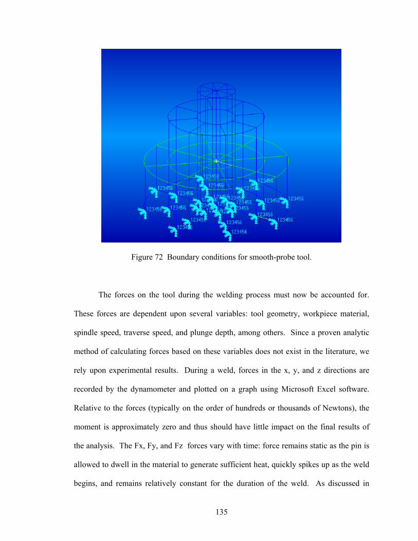
Figure 72 Boundary conditions for smooth-probe tool.
The forces on the tool during the welding process must now be accounted for.
These forces are dependent upon several variables: tool geometry, workpiece material,
spindle speed, traverse speed, and plunge depth, among others. Since a proven analytic
method of calculating forces based on these variables does not exist in the literature, we
rely upon experimental results. During a weld, forces in the x, y, and z directions are
recorded by the dynamometer and plotted on a graph using Microsoft Excel software.
Relative to the forces (typically on the order of hundreds or thousands of Newtons), the
moment is approximately zero and thus should have little impact on the final results of
the analysis. The Fx, Fy, and Fz forces vary with time: force remains static as the pin is
allowed to dwell in the material to generate sufficient heat, quickly spikes up as the weld
begins, and remains relatively constant for the duration of the weld. As discussed in
135
chapter IV, the average of the data recorded by the dynamometer during the steady-state
portion of the weld was used to obtain values for the Fx, Fy, and Fz values applied to the
tool.
In PATRAN, we can apply Fx, Fy, and Fz as pressures or forces to the tool
surface. The advantage of a pressure application is that it results in continuous stress
contours. When the forces are applied as is, the result is a stress concentration only at the
points of force application; the remainder of the mesh is white (the color used by the
PATRAN post processor to denote little or no stress). The application of forces instead
of pressure should have no negative impact on the model’s accuracy. The choice to apply
pressures is largely an aesthetic one; the continuous stress contours which result from
pressure application are more intuitive than the concentrated stresses produced by force
application.
To apply the forces as pressures, simply divide the force data by the surface area
(excluding portions of the tool which do not contact the material). The surface area
calculation can thus be broken down into the surface area of the probe summed with the
remaining radial area of the shoulder face. For the smooth probe tool, the surface area is
equal to approximately .35 in2. Note that forces must be converted from Newtons to
pounds to remain consistent with the dimensions of the tool, which were specified in
inches. Table 21 displays forces and pressures for the parameters considered for the
smooth probe steel tool. Table 22 reports the same data for the smooth probe tool with
diamond coating. Significantly more simulations were run for the coated tool on Al 6061
than for the uncoated tool. In the former case, it is anticipated that more simulations will
136
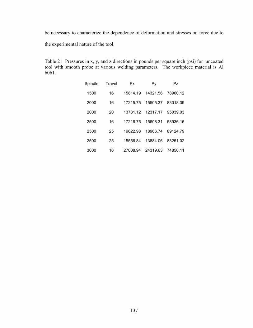
be necessary to characterize the dependence of deformation and stresses on force due to
the experimental nature of the tool.
Table 21 Pressures in x, y, and z directions in pounds per square inch (psi) for uncoated tool with smooth probe at various welding parameters. The workpiece material is Al 6061.
Spindle Travel Px Py Pz
1500 16 15814.19 14321.56 78960.12
2000 16 17215.75 15505.37 83018.39
2000 20 13781.12 12317.17 95039.03
2500 16 17216.75 15608.31 58936.16
2500 25 19622.98 18966.74 89124.79
2500 25 15556.84 13884.06 83251.02
3000 16 27008.94 24319.63 74850.11
137
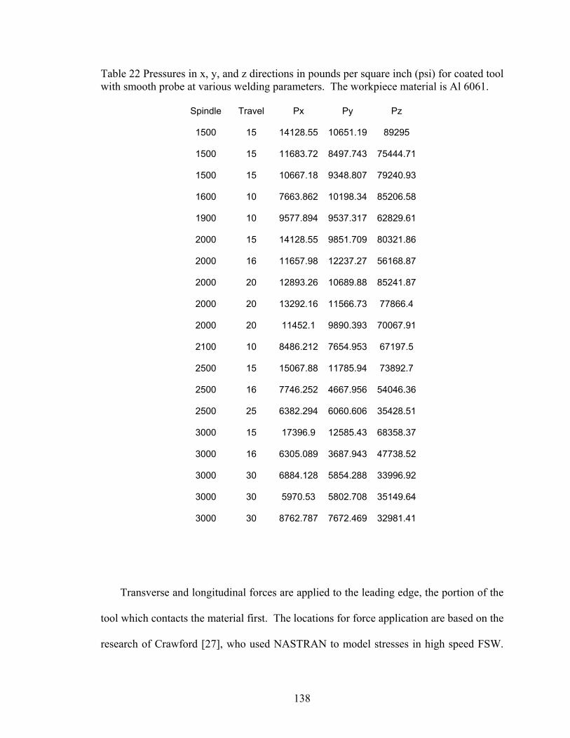
Table 22 Pressures in x, y, and z directions in pounds per square inch (psi) for coated tool with smooth probe at various welding parameters. The workpiece material is Al 6061.
Spindle Travel Px Py Pz
1500 15 14128.55 10651.19 89295
1500 15 11683.72 8497.743 75444.71
1500 15 10667.18 9348.807 79240.93
1600 10 7663.862 10198.34 85206.58
1900 10 9577.894 9537.317 62829.61
2000 15 14128.55 9851.709 80321.86
2000 16 11657.98 12237.27 56168.87
2000 20 12893.26 10689.88 85241.87
2000 20 13292.16 11566.73 77866.4
2000 20 11452.1 9890.393 70067.91
2100 10 8486.212 7654.953 67197.5
2500 15 15067.88 11785.94 73892.7
2500 16 7746.252 4667.956 54046.36
2500 25 6382.294 6060.606 35428.51
3000 15 17396.9 12585.43 68358.37
3000 16 6305.089 3687.943 47738.52
3000 30 6884.128 5854.288 33996.92
3000 30 5970.53 5802.708 35149.64
3000 30 8762.787 7672.469 32981.41
Transverse and longitudinal forces are applied to the leading edge, the portion of the
tool which contacts the material first. The locations for force application are based on the
research of Crawford [27], who used NASTRAN to model stresses in high speed FSW.
138
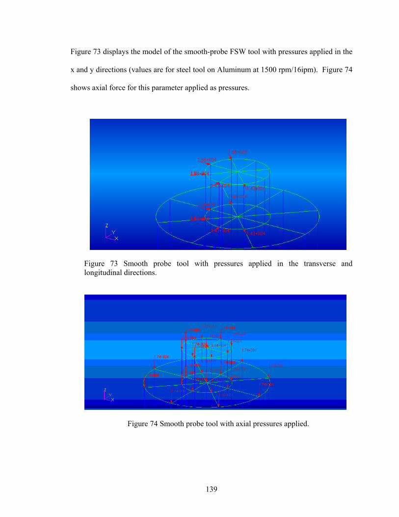
Figure 73 displays the model of the smooth-probe FSW tool with pressures applied in the
x and y directions (values are for steel tool on Aluminum at 1500 rpm/16ipm). Figure 74
shows axial force for this parameter applied as pressures.
Figure 73 Smooth probe tool with pressures applied in the transverse and longitudinal directions.
Figure 74 Smooth probe tool with axial pressures applied.
139
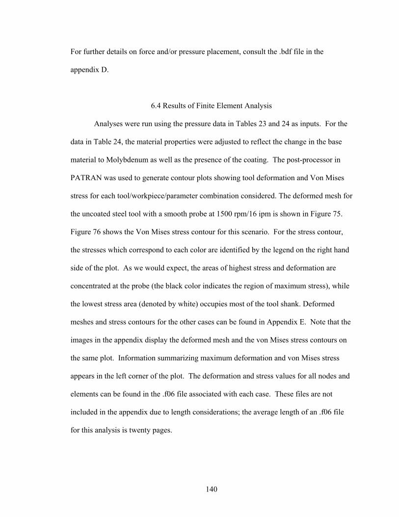
For further details on force and/or pressure placement, consult the .bdf file in the
appendix D.
6.4 Results of Finite Element Analysis
Analyses were run using the pressure data in Tables 23 and 24 as inputs. For the
data in Table 24, the material properties were adjusted to reflect the change in the base
material to Molybdenum as well as the presence of the coating. The post-processor in
PATRAN was used to generate contour plots showing tool deformation and Von Mises
stress for each tool/workpiece/parameter combination considered. The deformed mesh for
the uncoated steel tool with a smooth probe at 1500 rpm/16 ipm is shown in Figure 75.
Figure 76 shows the Von Mises stress contour for this scenario. For the stress contour,
the stresses which correspond to each color are identified by the legend on the right hand
side of the plot. As we would expect, the areas of highest stress and deformation are
concentrated at the probe (the black color indicates the region of maximum stress), while
the lowest stress area (denoted by white) occupies most of the tool shank. Deformed
meshes and stress contours for the other cases can be found in Appendix E. Note that the
images in the appendix display the deformed mesh and the von Mises stress contours on
the same plot. Information summarizing maximum deformation and von Mises stress
appears in the left corner of the plot. The deformation and stress values for all nodes and
elements can be found in the .f06 file associated with each case. These files are not
included in the appendix due to length considerations; the average length of an .f06 file
for this analysis is twenty pages.
140
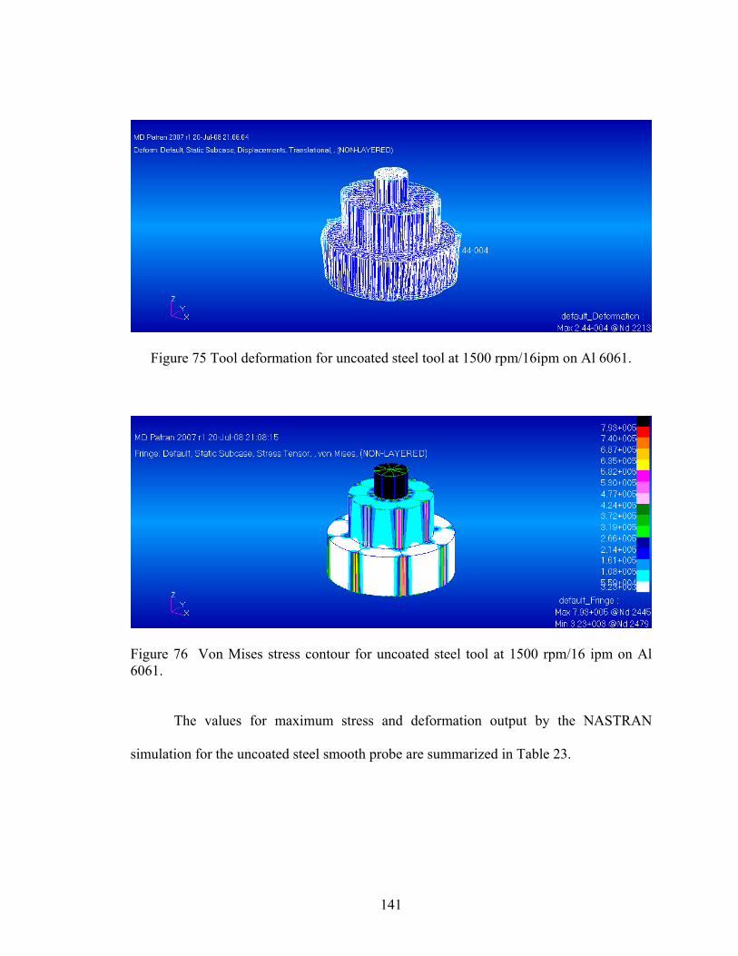
Figure 75 Tool deformation for uncoated steel tool at 1500 rpm/16ipm on Al 6061.
Figure 76 Von Mises stress contour for uncoated steel tool at 1500 rpm/16 ipm on Al 6061.
The values for maximum stress and deformation output by the NASTRAN
simulation for the uncoated steel smooth probe are summarized in Table 23.
141
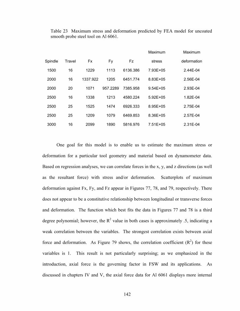
Table 23 Maximum stress and deformation predicted by FEA model for uncoated smooth probe steel tool on Al 6061.
Spindle Travel Fx Fy Fz
Maximum
stress
Maximum
deformation
1500 16 1229 1113 6136.386 7.93E+05 2.44E-04
2000 16 1337.922 1205 6451.774 8.83E+05 2.56E-04
2000 20 1071 957.2289 7385.958 9.54E+05 2.93E-04
2500 16 1338 1213 4580.224 5.92E+05 1.82E-04
2500 25 1525 1474 6926.333 8.95E+05 2.75E-04
2500 25 1209 1079 6469.853 8.36E+05 2.57E-04
3000 16 2099 1890 5816.976 7.51E+05 2.31E-04
One goal for this model is to enable us to estimate the maximum stress or
deformation for a particular tool geometry and material based on dynamometer data.
Based on regression analyses, we can correlate forces in the x, y, and z directions (as well
as the resultant force) with stress and/or deformation. Scatterplots of maximum
deformation against Fx, Fy, and Fz appear in Figures 77, 78, and 79, respectively. There
does not appear to be a constitutive relationship between longitudinal or transverse forces
and deformation. The function which best fits the data in Figures 77 and 78 is a third
degree polynomial; however, the R2 value in both cases is approximately .5, indicating a
weak correlation between the variables. The strongest correlation exists between axial
force and deformation. As Figure 79 shows, the correlation coefficient (R2) for these
variables is 1. This result is not particularly surprising; as we emphasized in the
introduction, axial force is the governing factor in FSW and its applications. As
discussed in chapters IV and V, the axial force data for Al 6061 displays more internal
142
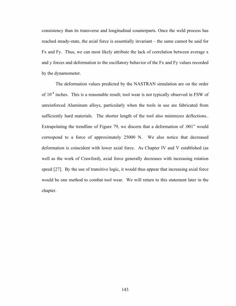
consistency than its transverse and longitudinal counterparts. Once the weld process has
reached steady-state, the axial force is essentially invariant – the same cannot be said for
Fx and Fy. Thus, we can most likely attribute the lack of correlation between average x
and y forces and deformation to the oscillatory behavior of the Fx and Fy values recorded
by the dynamometer.
The deformation values predicted by the NASTRAN simulation are on the order
of 10-4 inches. This is a reasonable result; tool wear is not typically observed in FSW of
unreinforced Aluminum alloys, particularly when the tools in use are fabricated from
sufficiently hard materials. The shorter length of the tool also minimizes deflections..
Extrapolating the trendline of Figure 79, we discern that a deformation of .001” would
correspond to a force of approximately 25000 N. We also notice that decreased
deformation is coincident with lower axial force. As Chapter IV and V established (as
well as the work of Crawford), axial force generally decreases with increasing rotation
speed [27]. By the use of transitive logic, it would thus appear that increasing axial force
would be one method to combat tool wear. We will return to this statement later in the
chapter.
143
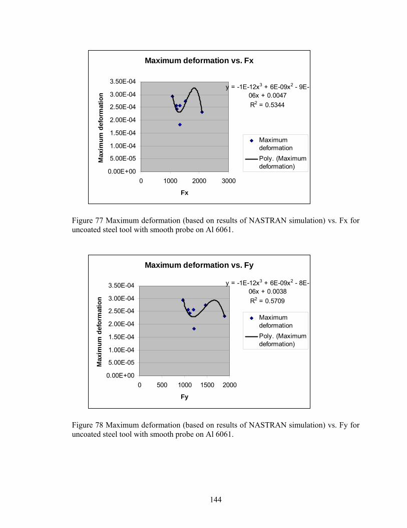
Maximum deformation vs. Fx
y = -1E-12x3 + 6E-09x2 - 9E-06x + 0.0047R2 = 0.5344
0.00E+00
5.00E-05
1.00E-04
1.50E-04
2.00E-04
2.50E-04
3.00E-04
3.50E-04
0 1000 2000 3000
Fx
Max
imum
def
orm
atio
n
MaximumdeformationPoly. (Maximumdeformation)
Figure 77 Maximum deformation (based on results of NASTRAN simulation) vs. Fx for uncoated steel tool with smooth probe on Al 6061.
Maximum deformation vs. Fy
y = -1E-12x3 + 6E-09x2 - 8E-06x + 0.0038R2 = 0.5709
0.00E+00
5.00E-05
1.00E-04
1.50E-04
2.00E-04
2.50E-04
3.00E-04
3.50E-04
0 500 1000 1500 2000
Fy
Max
imum
def
orm
atio
n
MaximumdeformationPoly. (Maximumdeformation)
Figure 78 Maximum deformation (based on results of NASTRAN simulation) vs. Fy for uncoated steel tool with smooth probe on Al 6061.
144
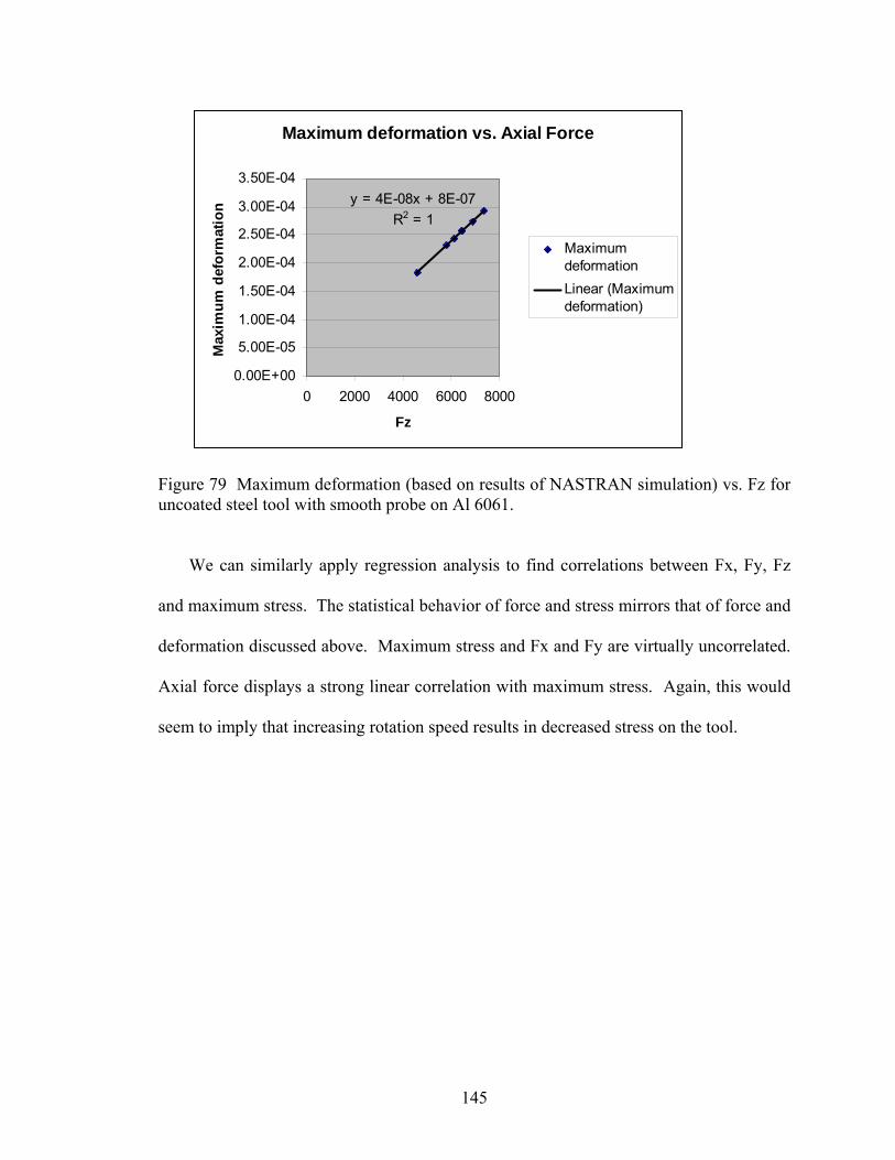
Maximum deformation vs. Axial Force
y = 4E-08x + 8E-07R2 = 1
0.00E+00
5.00E-05
1.00E-04
1.50E-04
2.00E-04
2.50E-04
3.00E-04
3.50E-04
0 2000 4000 6000 8000
Fz
Max
imum
def
orm
atio
n
MaximumdeformationLinear (Maximumdeformation)
Figure 79 Maximum deformation (based on results of NASTRAN simulation) vs. Fz for uncoated steel tool with smooth probe on Al 6061.
We can similarly apply regression analysis to find correlations between Fx, Fy, Fz
and maximum stress. The statistical behavior of force and stress mirrors that of force and
deformation discussed above. Maximum stress and Fx and Fy are virtually uncorrelated.
Axial force displays a strong linear correlation with maximum stress. Again, this would
seem to imply that increasing rotation speed results in decreased stress on the tool.
145
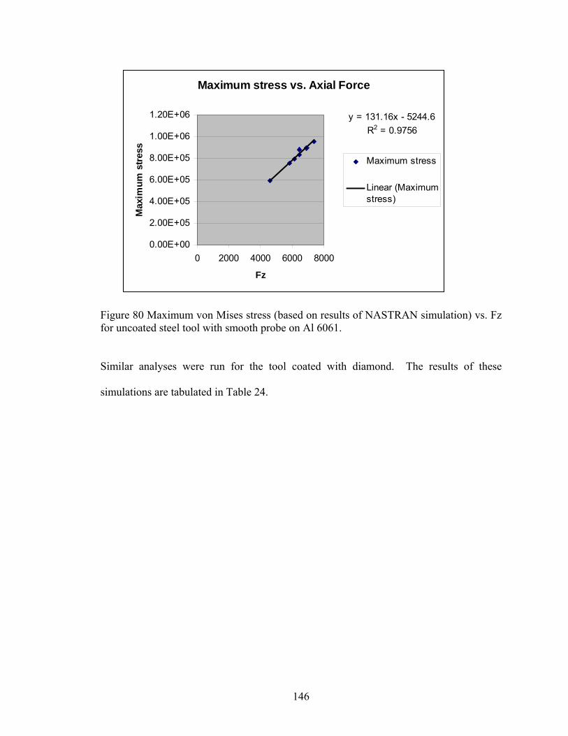
Maximum stress vs. Axial Force
y = 131.16x - 5244.6R2 = 0.9756
0.00E+00
2.00E+05
4.00E+05
6.00E+05
8.00E+05
1.00E+06
1.20E+06
0 2000 4000 6000 8000
Fz
Max
imum
stre
ss
Maximum stress
Linear (Maximumstress)
Figure 80 Maximum von Mises stress (based on results of NASTRAN simulation) vs. Fz for uncoated steel tool with smooth probe on Al 6061.
Similar analyses were run for the tool coated with diamond. The results of these
simulations are tabulated in Table 24.
146
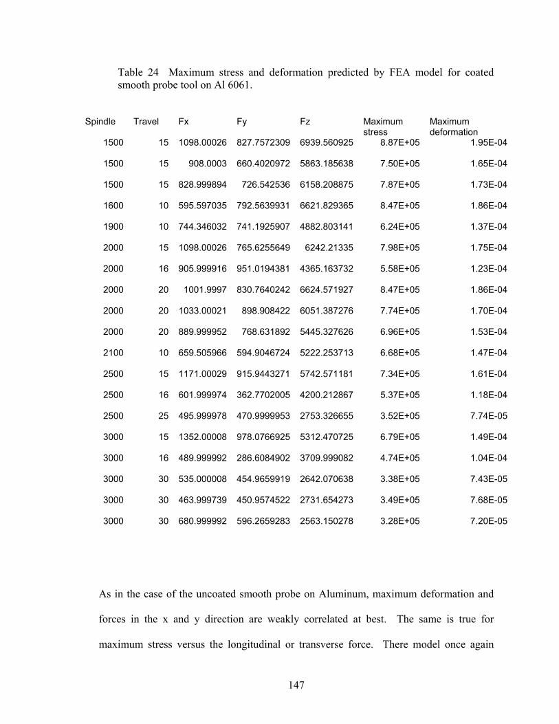
Table 24 Maximum stress and deformation predicted by FEA model for coated smooth probe tool on Al 6061.
Spindle Travel Fx Fy Fz Maximum stress
Maximum deformation
1500 15 1098.00026 827.7572309 6939.560925 8.87E+05 1.95E-04
1500 15 908.0003 660.4020972 5863.185638 7.50E+05 1.65E-04
1500 15 828.999894 726.542536 6158.208875 7.87E+05 1.73E-04
1600 10 595.597035 792.5639931 6621.829365 8.47E+05 1.86E-04
1900 10 744.346032 741.1925907 4882.803141 6.24E+05 1.37E-04
2000 15 1098.00026 765.6255649 6242.21335 7.98E+05 1.75E-04
2000 16 905.999916 951.0194381 4365.163732 5.58E+05 1.23E-04
2000 20 1001.9997 830.7640242 6624.571927 8.47E+05 1.86E-04
2000 20 1033.00021 898.908422 6051.387276 7.74E+05 1.70E-04
2000 20 889.999952 768.631892 5445.327626 6.96E+05 1.53E-04
2100 10 659.505966 594.9046724 5222.253713 6.68E+05 1.47E-04
2500 15 1171.00029 915.9443271 5742.571181 7.34E+05 1.61E-04
2500 16 601.999974 362.7702005 4200.212867 5.37E+05 1.18E-04
2500 25 495.999978 470.9999953 2753.326655 3.52E+05 7.74E-05
3000 15 1352.00008 978.0766925 5312.470725 6.79E+05 1.49E-04
3000 16 489.999992 286.6084902 3709.999082 4.74E+05 1.04E-04
3000 30 535.000008 454.9659919 2642.070638 3.38E+05 7.43E-05
3000 30 463.999739 450.9574522 2731.654273 3.49E+05 7.68E-05
3000 30 680.999992 596.2659283 2563.150278 3.28E+05 7.20E-05
As in the case of the uncoated smooth probe on Aluminum, maximum deformation and
forces in the x and y direction are weakly correlated at best. The same is true for
maximum stress versus the longitudinal or transverse force. There model once again
147
indicate a perfectly linear relationship between maximum deformation and axial force,
governed by the equation D = 3E-08Fz + 1E-07, where Fz is axial force in Newtons and
D is deformation in inches. The rate of change of deformation with force is the slope of
the trendline in Figure 81, 3E-08 in/N. Physically this means that a force increase of 1 N
corresponds to an increase in maximum deformation of 3E-08 inches. According to the
relationship established by this statistical correlation, a deformation of .001 inches
corresponds to a force of 33330 N. This is a significantly larger force value than that for
the uncoated tool at .001 inch deformation (approximately 25000 N). Though perhaps an
obvious result, the FEA model indicates that it requires more force to deform the coated
tool. A graphical comparison of maximum tool deformation as a function of axial force
for the coated and uncoated tool appears in Figure 82.
148
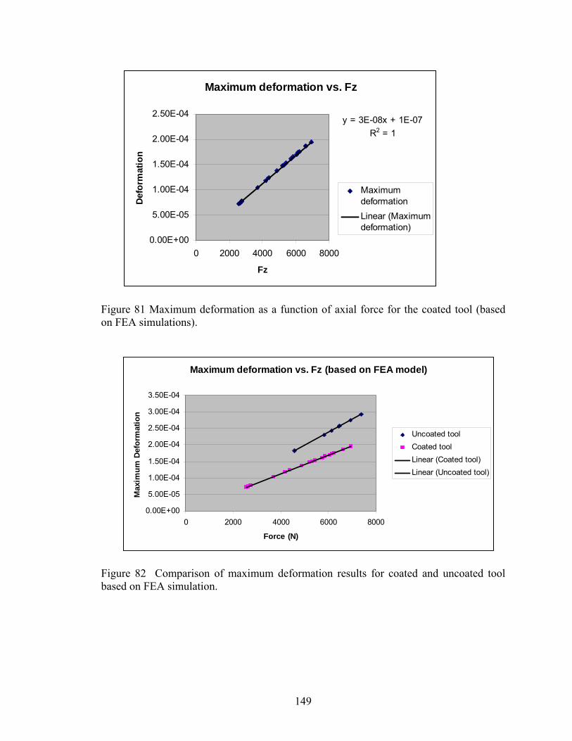
Maximum deformation vs. Fz
y = 3E-08x + 1E-07R2 = 1
0.00E+00
5.00E-05
1.00E-04
1.50E-04
2.00E-04
2.50E-04
0 2000 4000 6000 8000
Fz
Defo
rmat
ion
MaximumdeformationLinear (Maximumdeformation)
Figure 81 Maximum deformation as a function of axial force for the coated tool (based on FEA simulations).
Maximum deformation vs. Fz (based on FEA model)
0.00E+00
5.00E-05
1.00E-04
1.50E-04
2.00E-04
2.50E-04
3.00E-04
3.50E-04
0 2000 4000 6000 8000
Force (N)
Max
imum
Def
orm
atio
n
Uncoated toolCoated toolLinear (Coated tool)Linear (Uncoated tool)
Figure 82 Comparison of maximum deformation results for coated and uncoated tool based on FEA simulation.
149
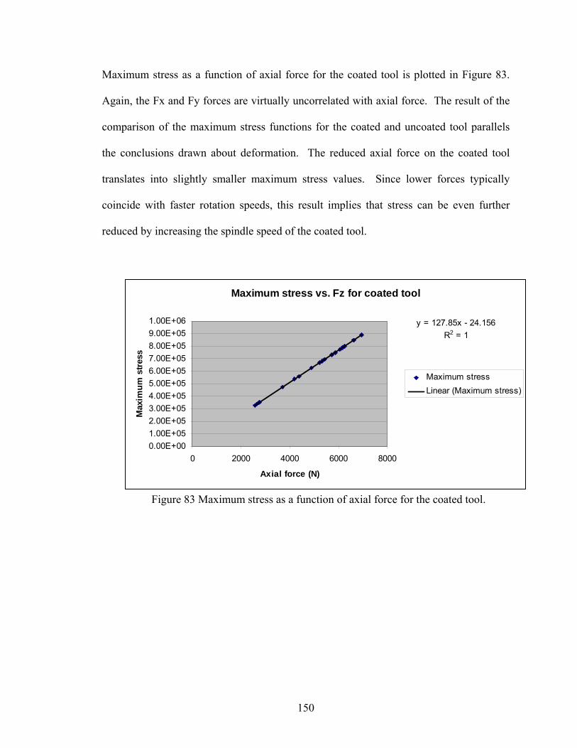
Maximum stress as a function of axial force for the coated tool is plotted in Figure 83.
Again, the Fx and Fy forces are virtually uncorrelated with axial force. The result of the
comparison of the maximum stress functions for the coated and uncoated tool parallels
the conclusions drawn about deformation. The reduced axial force on the coated tool
translates into slightly smaller maximum stress values. Since lower forces typically
coincide with faster rotation speeds, this result implies that stress can be even further
reduced by increasing the spindle speed of the coated tool.
Maximum stress vs. Fz for coated tool
y = 127.85x - 24.156R2 = 1
0.00E+001.00E+052.00E+053.00E+054.00E+055.00E+056.00E+057.00E+058.00E+059.00E+051.00E+06
0 2000 4000 6000 8000
Axial force (N)
Max
imum
stre
ss
Maximum stressLinear (Maximum stress)
Figure 83 Maximum stress as a function of axial force for the coated tool.
150
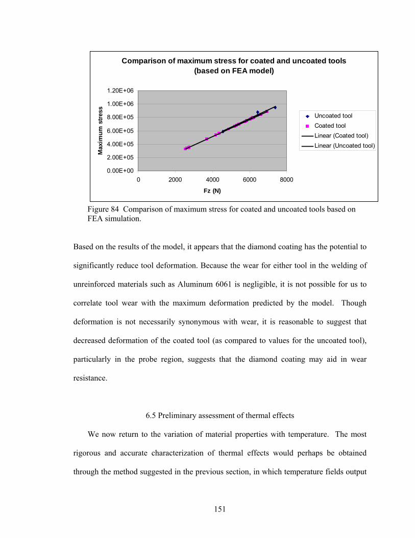
Comparison of maximum stress for coated and uncoated tools (based on FEA model)
0.00E+00
2.00E+05
4.00E+05
6.00E+05
8.00E+05
1.00E+06
1.20E+06
0 2000 4000 6000 8000
Fz (N)
Max
imum
str
ess
Uncoated toolCoated toolLinear (Coated tool)Linear (Uncoated tool)
Figure 84 Comparison of maximum stress for coated and uncoated tools based on FEA simulation.
Based on the results of the model, it appears that the diamond coating has the potential to
significantly reduce tool deformation. Because the wear for either tool in the welding of
unreinforced materials such as Aluminum 6061 is negligible, it is not possible for us to
correlate tool wear with the maximum deformation predicted by the model. Though
deformation is not necessarily synonymous with wear, it is reasonable to suggest that
decreased deformation of the coated tool (as compared to values for the uncoated tool),
particularly in the probe region, suggests that the diamond coating may aid in wear
resistance.
6.5 Preliminary assessment of thermal effects
We now return to the variation of material properties with temperature. The most
rigorous and accurate characterization of thermal effects would perhaps be obtained
through the method suggested in the previous section, in which temperature fields output
151
by FLUENT are used to determine the input of material properties in PATRAN.
However, a simpler protocol to analyze the effects of temperature variation on the
deformation and maximum stress for the coated and uncoated tool can be implemented in
PATRAN using the structure of the existing model. As discussed earlier in the chapter,
the modulus of elasticity for a particular material can decrease substantially with
increasing temperature. We would expect that such a decrease in elastic modulus would
result in increased deformation and maximum stress. In this sense, the results for the
smooth probe models presented previously may be underestimations. We can quantify
the model’s tendency to underpredict by re-running the analyses with the material moduli
adjusted to correspond with a typical welding temperature for FSW (for instance, 400
oC). The variability of the modulus of h13 tool steel was determined using data from
reference 4. At 427 oC, the elastic modulus of tool steel is reduced by approximately
twenty percent. The simulations of Figure 23 were run again with this reduced modulus
for steel as a material property input. The image of the deformed mesh and stress
contours for these simulations appear in the appendix. The function which governs
maximum deformation for the high temperature case is plotted in Figure 85. The
trendline which was the result of the analysis run using the value for the elastic modulus
at room temperature also appears for comparison. The graph makes it apparent that a
percent reduction in the modulus to reflect temperature changes translates into an
equivalent percent increase in deformation. The slope of the trendline for the data with a
modulus at 400 degrees Celsius is also steeper (5E-08 in/N) than that for the modulus at
room temperature (3E-08 in/N). Physically, this indicates that for the same amount of
force increase, the model which uses the modulus at 400 C as an input will experience a
152
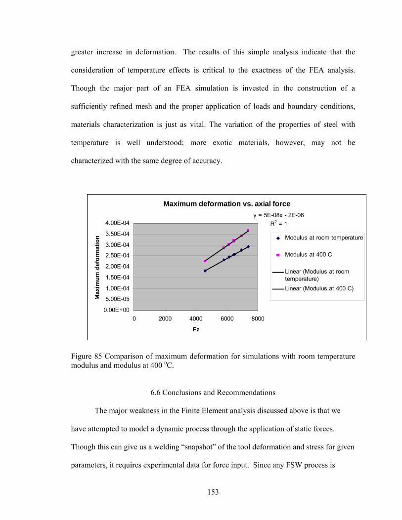
greater increase in deformation. The results of this simple analysis indicate that the
consideration of temperature effects is critical to the exactness of the FEA analysis.
Though the major part of an FEA simulation is invested in the construction of a
sufficiently refined mesh and the proper application of loads and boundary conditions,
materials characterization is just as vital. The variation of the properties of steel with
temperature is well understood; more exotic materials, however, may not be
characterized with the same degree of accuracy.
Maximum deformation vs. axial forcey = 5E-08x - 2E-06
R2 = 1
0.00E+00
5.00E-05
1.00E-04
1.50E-04
2.00E-04
2.50E-04
3.00E-04
3.50E-04
4.00E-04
0 2000 4000 6000 8000
Fz
Max
imum
def
orm
atio
n Modulus at room temperature
Modulus at 400 C
Linear (Modulus at roomtemperature)Linear (Modulus at 400 C)
Figure 85 Comparison of maximum deformation for simulations with room temperature modulus and modulus at 400 oC.
6.6 Conclusions and Recommendations
The major weakness in the Finite Element analysis discussed above is that we
have attempted to model a dynamic process through the application of static forces.
Though this can give us a welding “snapshot” of the tool deformation and stress for given
parameters, it requires experimental data for force input. Since any FSW process is
153
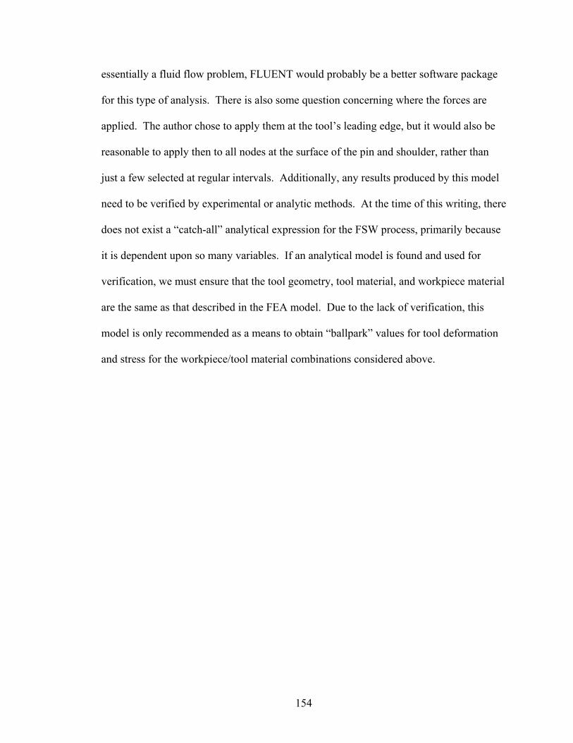
essentially a fluid flow problem, FLUENT would probably be a better software package
for this type of analysis. There is also some question concerning where the forces are
applied. The author chose to apply them at the tool’s leading edge, but it would also be
reasonable to apply then to all nodes at the surface of the pin and shoulder, rather than
just a few selected at regular intervals. Additionally, any results produced by this model
need to be verified by experimental or analytic methods. At the time of this writing, there
does not exist a “catch-all” analytical expression for the FSW process, primarily because
it is dependent upon so many variables. If an analytical model is found and used for
verification, we must ensure that the tool geometry, tool material, and workpiece material
are the same as that described in the FEA model. Due to the lack of verification, this
model is only recommended as a means to obtain “ballpark” values for tool deformation
and stress for the workpiece/tool material combinations considered above.
154
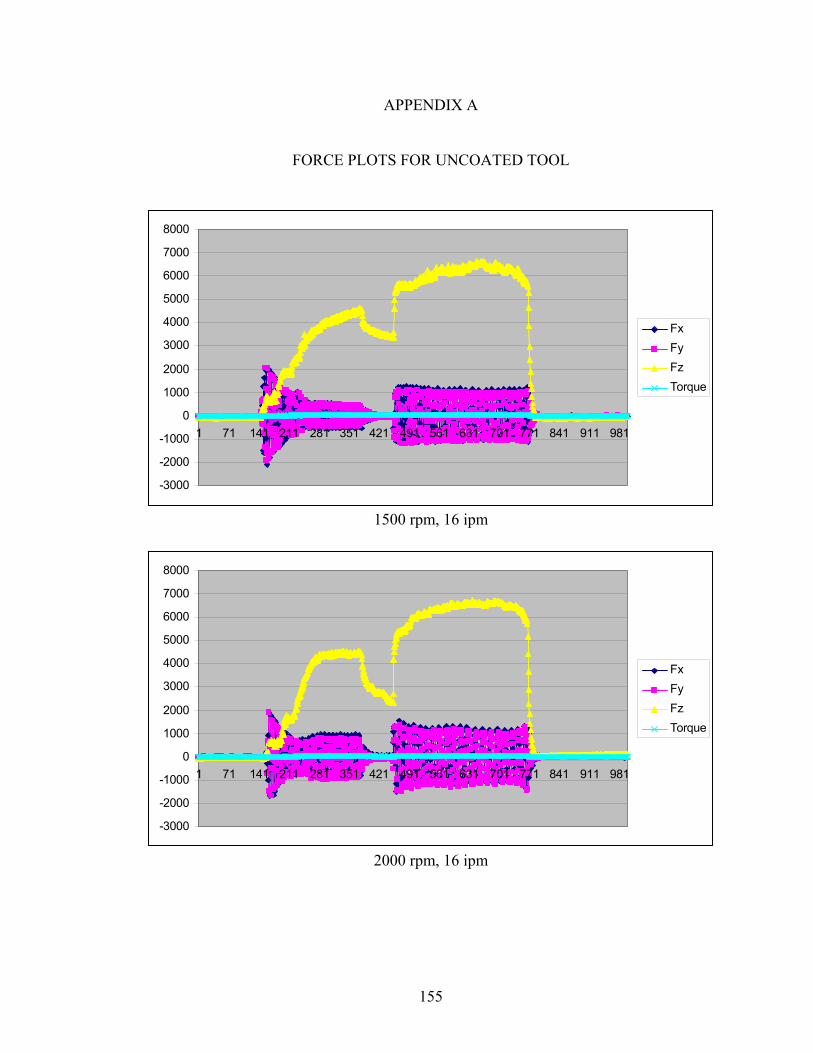
APPENDIX A
FORCE PLOTS FOR UNCOATED TOOL
-3000
-2000
-1000
0
1000
2000
3000
4000
5000
6000
7000
8000
1 71 141 211 281 351 421 491 561 631 701 771 841 911 981
FxFyFzTorque
1500 rpm, 16 ipm
-3000
-2000
-1000
0
1000
2000
3000
4000
5000
6000
7000
8000
1 71 141 211 281 351 421 491 561 631 701 771 841 911 981
FxFyFzTorque
2000 rpm, 16 ipm
155
-4000
-2000
0
2000
4000
6000
8000
10000
1 85 169 253 337 421 505 589 673 757 841 925 1009 1093 1177
FxFyFzTorque
2000 rpm, 20 ipm
-2000
-1000
0
1000
2000
3000
4000
5000
6000
1 71 141 211 281 351 421 491 561 631 701 771 841 911 981
FxFyFzTorque
2500 rpm, 16 ipm
156
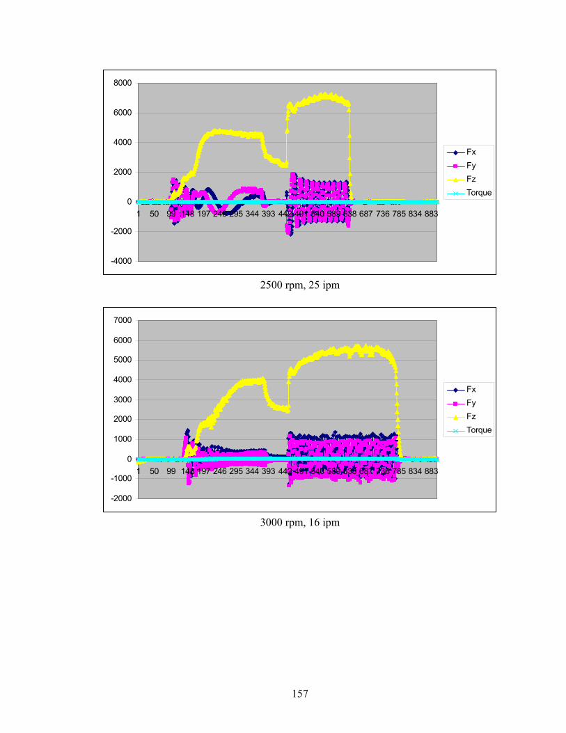
-4000
-2000
0
2000
4000
6000
8000
1 50 99 148 197 246 295 344 393 442 491 540 589 638 687 736 785 834 883
FxFyFzTorque
2500 rpm, 25 ipm
-2000
-1000
0
1000
2000
3000
4000
5000
6000
7000
1 50 99 148 197 246 295 344 393 442 491 540 589 638 687 736 785 834 883
FxFyFzTorque
3000 rpm, 16 ipm
157

APPENDIX B
FORCE PLOTS FOR COATED TOOLS
-4000
-2000
0
2000
4000
6000
8000
1 50 99 148 197 246 295 344 393 442 491 540 589 638 687 736 785 834 883
FxFyFzTorque
1500 rpm, 16 ipm
-2000
-1000
0
1000
2000
3000
4000
5000
6000
7000
8000
1 201 401 601 801 1001 1201 1401 1601 1801 2001 2201 2401 2601 2801
FxFyFzTorque
1600 rpm, 10 ipm
158
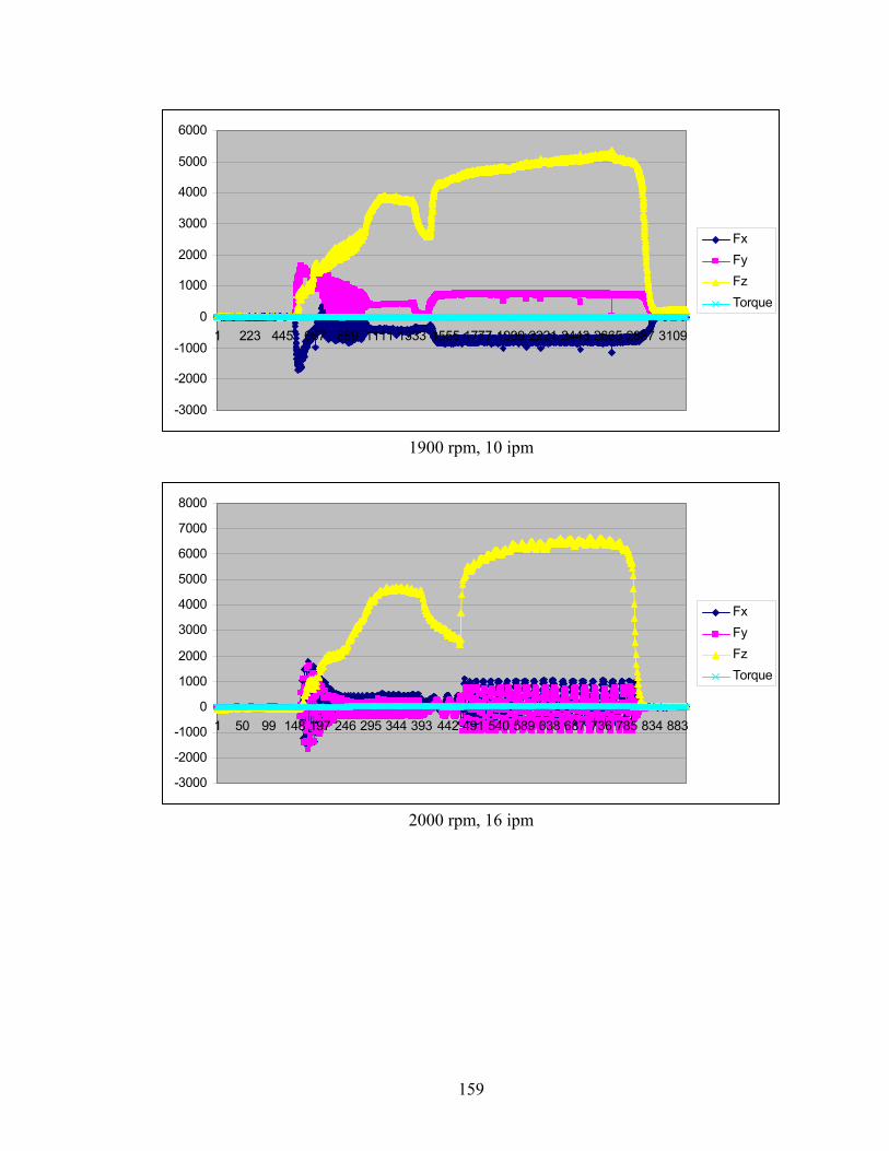
-3000
-2000
-1000
0
1000
2000
3000
4000
5000
6000
1 223 445 667 889 1111 1333 1555 1777 1999 2221 2443 2665 2887 3109
FxFyFzTorque
1900 rpm, 10 ipm
-3000
-2000
-1000
0
1000
2000
3000
4000
5000
6000
7000
8000
1 50 99 148 197 246 295 344 393 442 491 540 589 638 687 736 785 834 883
FxFyFzTorque
2000 rpm, 16 ipm
159
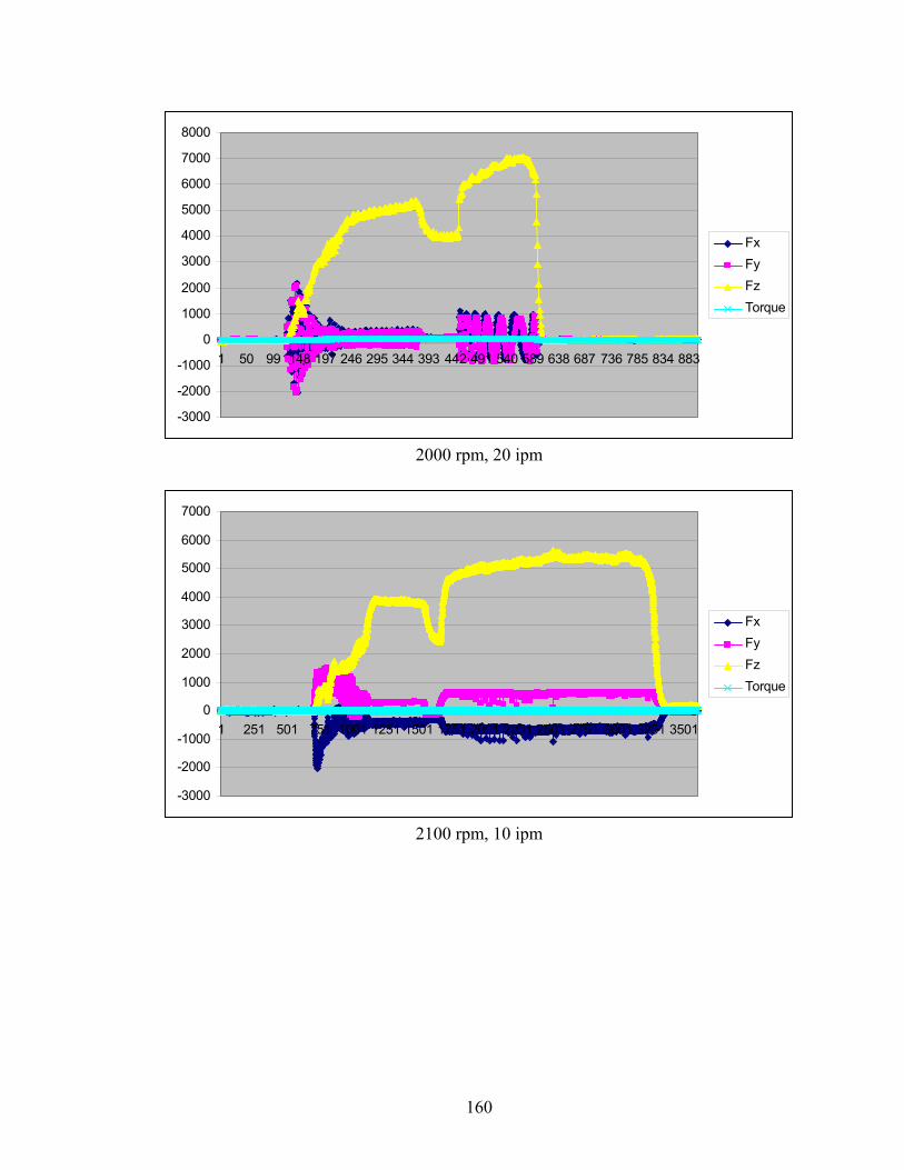
-3000
-2000
-1000
0
1000
2000
3000
4000
5000
6000
7000
8000
1 50 99 148 197 246 295 344 393 442 491 540 589 638 687 736 785 834 883
FxFyFzTorque
2000 rpm, 20 ipm
-3000
-2000
-1000
0
1000
2000
3000
4000
5000
6000
7000
1 251 501 751 1001 1251 1501 1751 2001 2251 2501 2751 3001 3251 3501
FxFyFzTorque
2100 rpm, 10 ipm
160
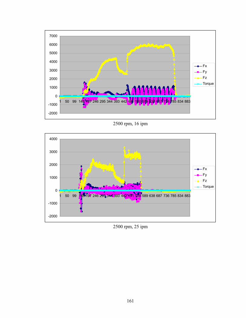
-2000
-1000
0
1000
2000
3000
4000
5000
6000
7000
1 50 99 148 197 246 295 344 393 442 491 540 589 638 687 736 785 834 883
FxFyFzTorque
2500 rpm, 16 ipm
-2000
-1000
0
1000
2000
3000
4000
1 50 99 148 197 246 295 344 393 442 491 540 589 638 687 736 785 834 883
FxFyFzTorque
2500 rpm, 25 ipm
161
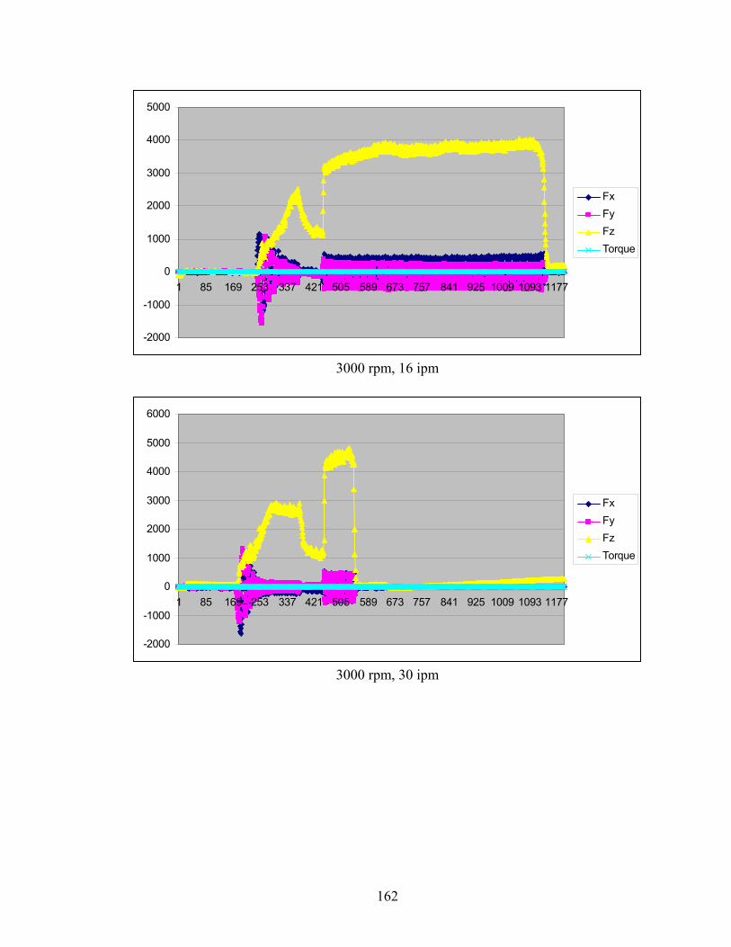
-2000
-1000
0
1000
2000
3000
4000
5000
1 85 169 253 337 421 505 589 673 757 841 925 1009 1093 1177
FxFyFzTorque
3000 rpm, 16 ipm
-2000
-1000
0
1000
2000
3000
4000
5000
6000
1 85 169 253 337 421 505 589 673 757 841 925 1009 1093 1177
FxFyFzTorque
3000 rpm, 30 ipm
162
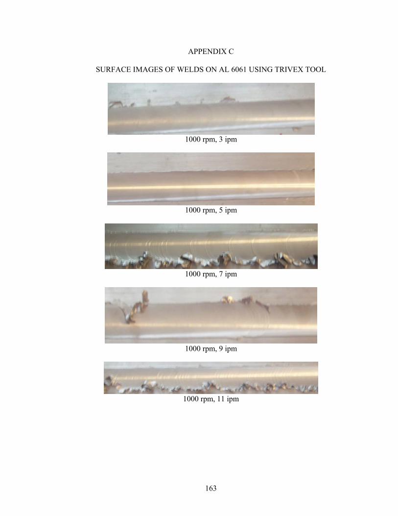
APPENDIX C
SURFACE IMAGES OF WELDS ON AL 6061 USING TRIVEX TOOL
1000 rpm, 3 ipm
1000 rpm, 5 ipm
1000 rpm, 7 ipm
1000 rpm, 9 ipm
1000 rpm, 11 ipm
163

1500 rpm, 5 ipm
1500 rpm, 7 ipm
1500 rpm, 9 ipm
1500 rpm, 11 ipm
1500 rpm, 13 ipm
2000 rpm, 7 ipm
164
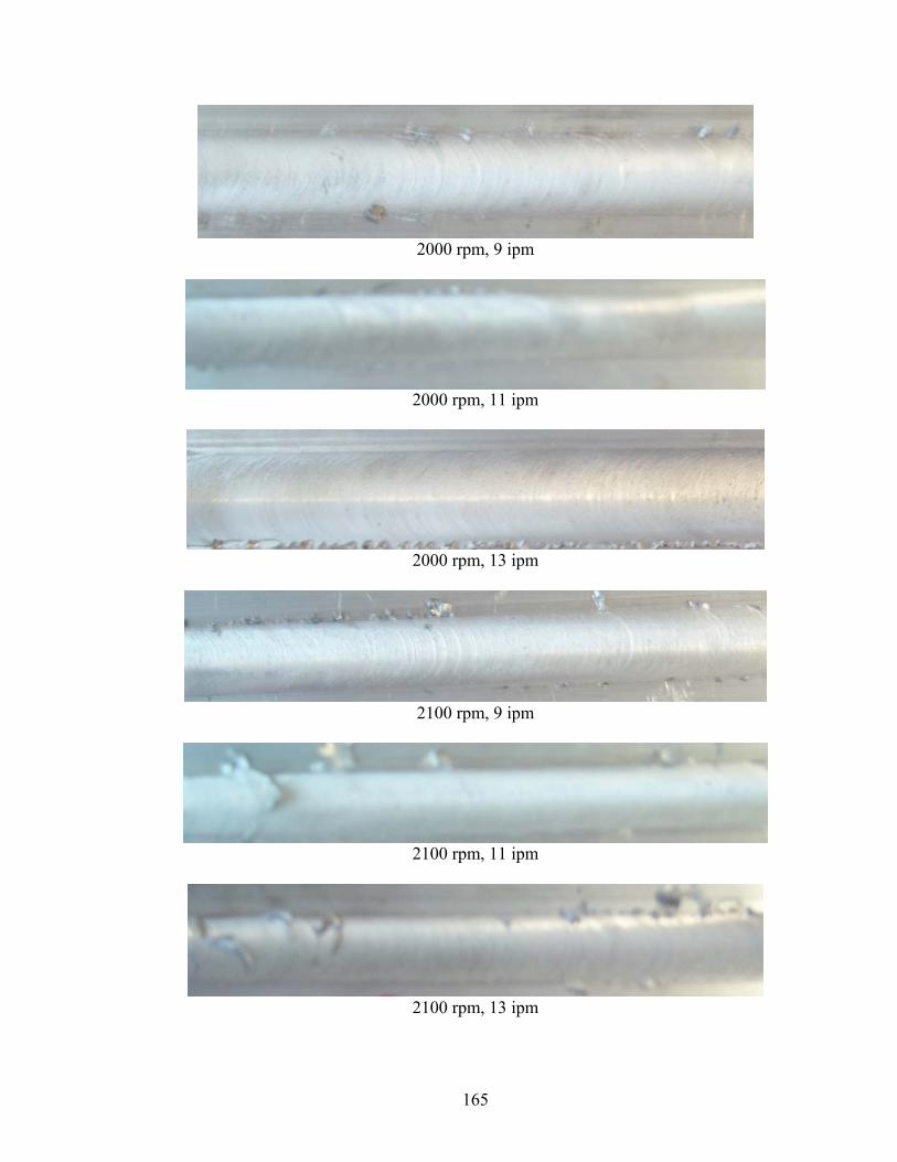
2000 rpm, 9 ipm
2000 rpm, 11 ipm
2000 rpm, 13 ipm
2100 rpm, 9 ipm
2100 rpm, 11 ipm
2100 rpm, 13 ipm
165
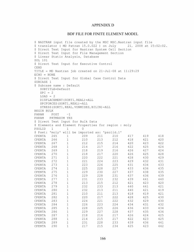
APPENDIX D
BDF FILE FOR FINITE ELEMENT MODEL
$ NASTRAN input file created by the MSC MSC.Nastran input file $ translator ( MD Patran 15.0.022 ) on July 21, 2008 at 15:02:02. $ Direct Text Input for Nastran System Cell Section $ Direct Text Input for File Management Section $ Linear Static Analysis, Database SOL 101 $ Direct Text Input for Executive Control CEND TITLE = MD Nastran job created on 21-Jul-08 at 11:29:29 ECHO = NONE $ Direct Text Input for Global Case Control Data SUBCASE 1 $ Subcase name : Default SUBTITLE=Default SPC = 2 LOAD = 2 DISPLACEMENT(SORT1,REAL)=ALL SPCFORCES(SORT1,REAL)=ALL STRESS(SORT1,REAL,VONMISES,BILIN)=ALL BEGIN BULK PARAM POST -1 PARAM PRTMAXIM YES $ Direct Text Input for Bulk Data $ Elements and Element Properties for region : moly PSOLID 1 1 0 $ Pset: "moly" will be imported as: "psolid.1" CPENTA 265 1 209 211 210 417 419 418 CPENTA 266 1 210 213 212 418 421 420 CPENTA 267 1 212 215 214 420 423 422 CPENTA 268 1 214 217 216 422 425 424 CPENTA 269 1 218 219 216 426 427 424 CPENTA 270 1 218 217 220 426 425 428 CPENTA 271 1 220 222 221 428 430 429 CPENTA 272 1 221 224 223 429 432 431 CPENTA 273 1 223 226 225 431 434 433 CPENTA 274 1 225 228 227 433 436 435 CPENTA 275 1 229 230 227 437 438 435 CPENTA 276 1 229 228 231 437 436 439 CPENTA 277 1 231 233 232 439 441 440 CPENTA 278 1 213 215 212 421 423 420 CPENTA 279 1 232 233 213 440 441 421 CPENTA 280 1 232 213 211 440 421 419 CPENTA 281 1 210 211 213 418 419 421 CPENTA 282 1 220 217 222 428 425 430 CPENTA 283 1 224 221 222 432 429 430 CPENTA 284 1 226 223 224 434 431 432 CPENTA 285 1 228 225 226 436 433 434 CPENTA 286 1 229 227 228 437 435 436 CPENTA 287 1 218 216 217 426 424 425 CPENTA 288 1 214 215 217 422 423 425 CPENTA 289 1 231 228 233 439 436 441 CPENTA 290 1 217 215 234 425 423 442
166
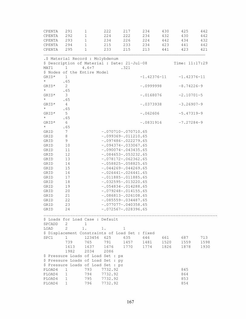
CPENTA 291 1 222 217 234 430 425 442 CPENTA 292 1 224 222 234 432 430 442 CPENTA 293 1 234 226 224 442 434 432 CPENTA 294 1 215 233 234 423 441 442 CPENTA 295 1 233 215 213 441 423 421 ………………………………………………………………………………………………………………………………………………………………………………… .$ Material Record : Molybdenum $ Description of Material : Date: 21-Jul-08 Time: 11:17:29 MAT1 1 4.6+7 .321 $ Nodes of the Entire Model GRID* 1 -1.42376-11 -1.42376-11 * .65 GRID* 2 -.0999998 -8.74226-9 * .65 GRID* 3 -.0168076 -2.10701-5 * .65 GRID* 4 -.0373938 -3.26907-9 * .65 GRID* 5 -.062606 -5.47319-9 * .65 GRID* 6 -.0831916 -7.27284-9 * .65 GRID 7 -.070710-.070710.65 GRID 8 -.099369-.011210.65 GRID 9 -.097486-.022279.65 GRID 10 -.094374-.033067.65 GRID 11 -.090074-.043435.65 GRID 12 -.084653-.053232.65 GRID 13 -.078172-.062362.65 GRID 14 -.058825-.058825.65 GRID 15 -.044269-.044269.65 GRID 16 -.026441-.026441.65 GRID 17 -.011885-.011885.65 GRID 18 -.032595-.013220.65 GRID 19 -.054834-.014288.65 GRID 20 -.079248-.014155.65 GRID 21 -.086813-.026108.65 GRID 22 -.085559-.034487.65 GRID 23 -.077077-.040358.65 GRID 24 -.072567-.028396.65 ……………………………………………………………………………………………… $ Loads for Load Case : Default SPCADD 2 1 LOAD 2 1. 1. 1 $ Displacement Constraints of Load Set : fixed SPC1 1 123456 625 635 646 661 687 713 739 765 791 1457 1481 1520 1559 1598 1613 1637 1676 1770 1774 1826 1878 1930 1982 2034 2086 $ Pressure Loads of Load Set : px $ Pressure Loads of Load Set : py $ Pressure Loads of Load Set : pz PLOAD4 1 793 7732.92 845 PLOAD4 1 794 7732.92 864 PLOAD4 1 795 7732.92 853 PLOAD4 1 796 7732.92 854
167
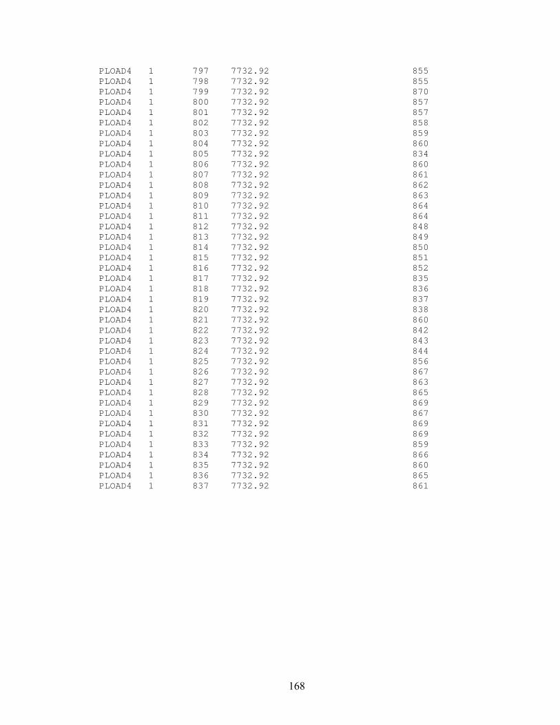
PLOAD4 1 797 7732.92 855 PLOAD4 1 798 7732.92 855 PLOAD4 1 799 7732.92 870 PLOAD4 1 800 7732.92 857 PLOAD4 1 801 7732.92 857 PLOAD4 1 802 7732.92 858 PLOAD4 1 803 7732.92 859 PLOAD4 1 804 7732.92 860 PLOAD4 1 805 7732.92 834 PLOAD4 1 806 7732.92 860 PLOAD4 1 807 7732.92 861 PLOAD4 1 808 7732.92 862 PLOAD4 1 809 7732.92 863 PLOAD4 1 810 7732.92 864 PLOAD4 1 811 7732.92 864 PLOAD4 1 812 7732.92 848 PLOAD4 1 813 7732.92 849 PLOAD4 1 814 7732.92 850 PLOAD4 1 815 7732.92 851 PLOAD4 1 816 7732.92 852 PLOAD4 1 817 7732.92 835 PLOAD4 1 818 7732.92 836 PLOAD4 1 819 7732.92 837 PLOAD4 1 820 7732.92 838 PLOAD4 1 821 7732.92 860 PLOAD4 1 822 7732.92 842 PLOAD4 1 823 7732.92 843 PLOAD4 1 824 7732.92 844 PLOAD4 1 825 7732.92 856 PLOAD4 1 826 7732.92 867 PLOAD4 1 827 7732.92 863 PLOAD4 1 828 7732.92 865 PLOAD4 1 829 7732.92 869 PLOAD4 1 830 7732.92 867 PLOAD4 1 831 7732.92 869 PLOAD4 1 832 7732.92 869 PLOAD4 1 833 7732.92 859 PLOAD4 1 834 7732.92 866 PLOAD4 1 835 7732.92 860 PLOAD4 1 836 7732.92 865 PLOAD4 1 837 7732.92 861
168
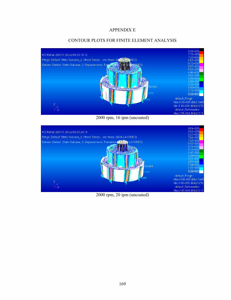
APPENDIX E
CONTOUR PLOTS FOR FINITE ELEMENT ANALYSIS
2000 rpm, 16 ipm (uncoated)
2000 rpm, 20 ipm (uncoated)
169
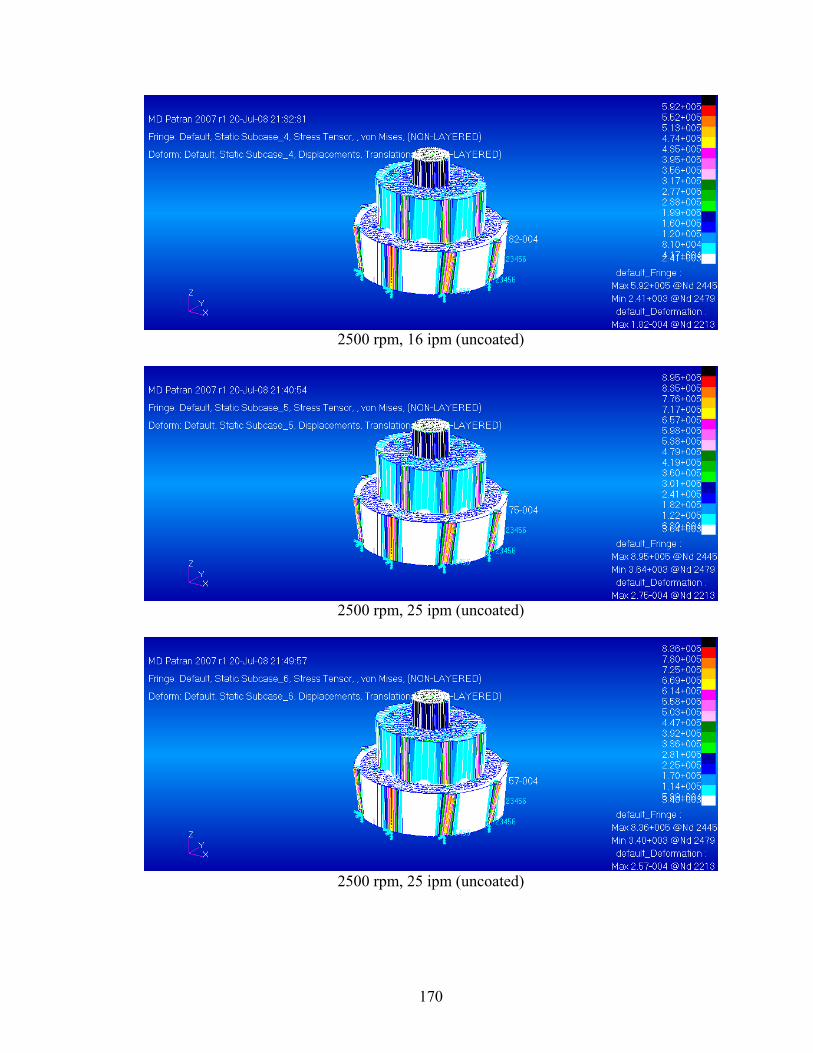
2500 rpm, 16 ipm (uncoated)
2500 rpm, 25 ipm (uncoated)
2500 rpm, 25 ipm (uncoated)
170
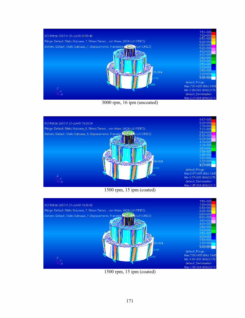
3000 rpm, 16 ipm (uncoated)
1500 rpm, 15 ipm (coated)
1500 rpm, 15 ipm (coated)
171
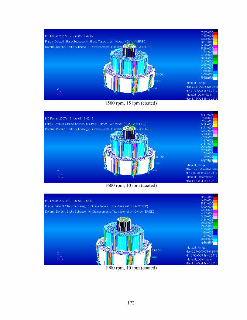
1500 rpm, 15 ipm (coated)
1600 rpm, 10 ipm (coated)
1900 rpm, 10 ipm (coated)
172
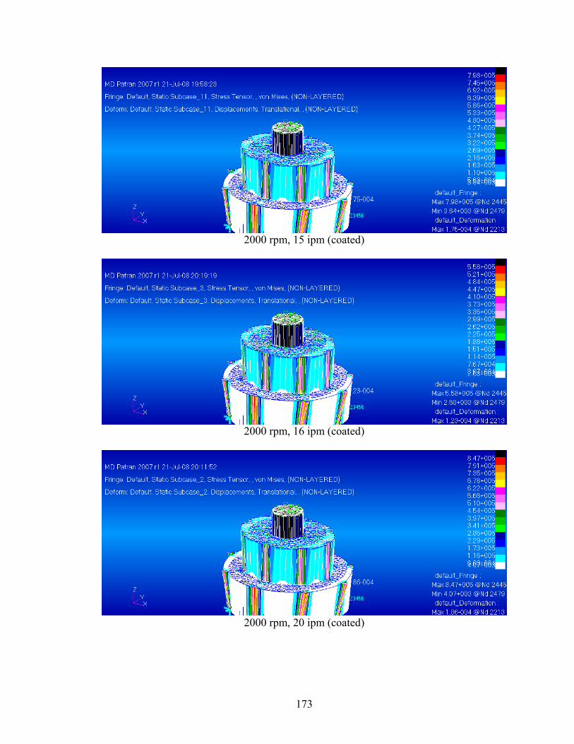
2000 rpm, 15 ipm (coated)
2000 rpm, 16 ipm (coated)
2000 rpm, 20 ipm (coated)
173
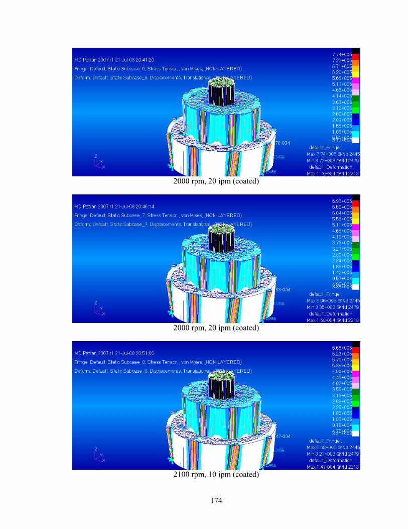
2000 rpm, 20 ipm (coated)
2000 rpm, 20 ipm (coated)
2100 rpm, 10 ipm (coated)
174

2500 rpm, 15 ipm (coated)
2500 rpm, 16 ipm (coated)
2500 rpm, 25 ipm (coated)
175

3000 rpm, 15 ipm (coated)
3000 rpm, 16 ipm (coated)
3000 rpm, 30 ipm (coated)
176
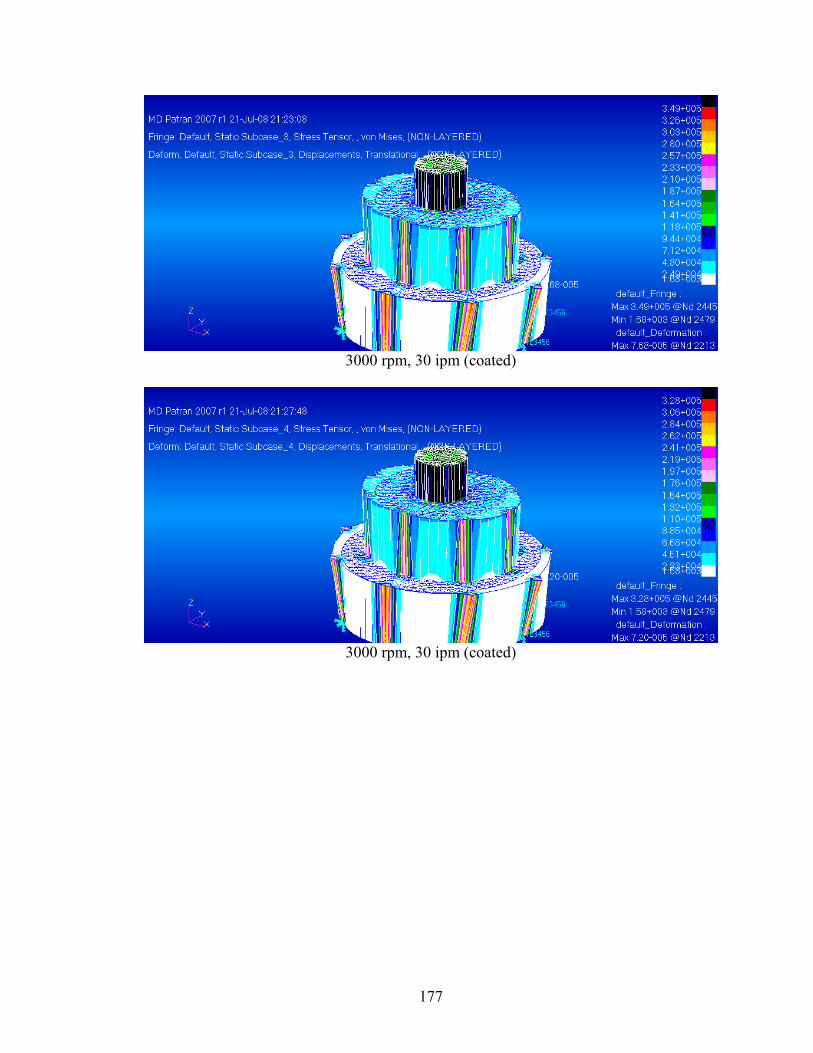
3000 rpm, 30 ipm (coated)
3000 rpm, 30 ipm (coated)
177
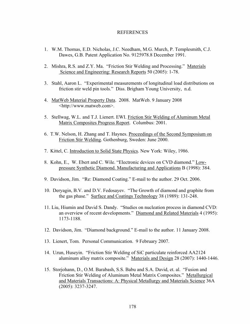
REFERENCES
1. W.M. Thomas, E.D. Nicholas, J.C. Needham, M.G. Murch, P. Templesmith, C.J. Dawes, G.B. Patent Application No. 9125978.8 December 1991. 2. Mishra, R.S. and Z.Y. Ma. “Friction Stir Welding and Processing.” Materials
Science and Engineering: Research Reports 50 (2005): 1-78.
3. Stahl, Aaron L. “Experimental measurements of longitudinal load distributions on friction stir weld pin tools.” Diss. Brigham Young University, n.d. 4. MatWeb Material Property Data. 2008. MatWeb. 9 January 2008 <http://www.matweb.com>. 5. Stellwag, W.L. and T.J. Lienert. EWI. Friction Stir Welding of Aluminum Metal
Matrix Composites Progress Report. Columbus: 2001.
6. T.W. Nelson, H. Zhang and T. Haynes. Proceedings of the Second Symposium on Friction Stir Welding. Gothenburg, Sweden: June 2000. 7. Kittel, C. Introduction to Solid State Physics. New York: Wiley, 1986.
8. Kohn, E., W. Ebert and C. Wile. “Electronic devices on CVD diamond.” Low-pressure Synthetic Diamond. Manufacturing and Applications B (1998): 384.
9. Davidson, Jim. “Re: Diamond Coating.” E-mail to the author. 29 Oct. 2006.
10. Deryagin, B.V. and D.V. Fedosayev. “The Growth of diamond and graphite from the gas phase.” Surface and Coatings Technology 38 (1989): 131-248.
11. Liu, Hiumin and David S. Dandy. “Studies on nucleation process in diamond CVD:
an overview of recent developments.” Diamond and Related Materials 4 (1995): 1173-1188.
12. Davidson, Jim. “Diamond background.” E-mail to the author. 11 January 2008.
13. Lienert, Tom. Personal Communication. 9 February 2007.
14. Uzun, Huseyin. “Friction Stir Welding of SiC particulate reinforced AA2124 aluminum alloy matrix composite.” Materials and Design 28 (2007): 1440-1446. 15. Storjohann, D., O.M. Barabash, S.S. Babu and S.A. David, et. al. “Fusion and
Friction Stir Welding of Aluminum Metal Matrix Composites.” Metallurgical and Materials Transactions: A: Physical Metallurgy and Materials Science 36A (2005): 3237-3247.
178
16. Dahotre, N.B., M.H. McCay, T.D. McCay, S. Gopinathan and L.F. Allard. “Pulse laser processing of a SiC/Al alloy metal matrix composite.” Journal of Materials Research 6 (1991): 514-29.
17. Lee, J.A., R.W. Carter and J. Ding. National Aeronautics and Space Administration.
Friction Stir Welding of Aluminum Metal Matrix Composites (MSFC Center Director’s Discretionary Fund Final Report, Project No. 98-09). Washington: GPO, 1998.
18. Diwan, Ravinder. National Aeronautics and Space Administration. Investigation of
Friction Stir Welding of Al Metal Matrix Composite Materials. Huntsville, AL: 2002.
19. Marzoli, L.M., A.V. Strombeck, J.F. Dos Santos, C. Gambaro and L.M. Volpone.
“Friction stir welding of an AA6061/Al2O3/20p reinforced alloy.” Composites Science and Technology 66 (2006): 363-371.
20. Ceschini, L., I. Boromei, G. Minak, A. Morri and F. Tarterini. “Microstructure,
tensile and fatigue properties of AA6061/20 vol.% Al2O3p friction stir welded joints.” Composites Part A: Applied Science and Manufacturing 38 (2007): 1200-1210.
21. Cavaliere, P., E. Cerri, L. Marzoli and J. Dos Santos. “Friction stir welding of
ceramic particle reinforced Aluminium based metal matrix composites.” Applied Composite Materials 11 (2004): 247-258.
22. Feng, A.H., B.L. Xiao, Z.Y. Ma. “Effect of microstructural evolution on mechanical
properties of friction stir welded AA2009/SiCp composite.” Composites Science and Technology (2008).
23. Humphreys, F.J. and M. Hatherly. Recrystallization and related annealing
phenomena. Pergamon, 1996. 24. Klug, H.P. and L.E. Alexander. X-ray diffraction procedures for polycrystalline and
amorphous materials. New York: Wiley, 1974. 25. Fernandez, G.J. and L.E. Murr. “Characterization of tool wear and weld
optimization in the friction-stir welding of cast aluminum 359+20% SiC metal matrix composite.” Materials Characterization 52 (2004): 65-75.
26. Prado, R.A., L.E. Murr, K.F. Soto and J.C. McClure. “Self-optimization in tool wear
for friction-stir welding of Al 6061+20% Al2O3 MMC.” Materials Science and Engineering 349 (2003): 156-165.
27. Crawford, Reginald. “A Mechanistic Study of the Friction Stir Welding Process.”
Diss. Vanderbilt University, August 2006.
179
28. Roy, G.G., R. Nandan, and T. DebRoy. “Dimensionless correlation to estimate peak temperature during friction stir welding.” Science and Technology of Welding and Joining 11 (2006): 606-608.
29. Lee, S.-Tong, Zhangda Lin, and Xin Jiang. “CVD Diamond Films: nucleation and
growth.” Materials Science and Engineering 25 (1999): 123-154. 30. Davidson, Jim. Personal Communication. 2 July 2008. 31. Mills, K.C. Recommended Values of Thermophysical Properties for Commercial
Alloys, Cambridge, UK: 2002. 32. Davidson, Jim. “Thermal conductivity of diamond.” E-mail to the author. 8 July
2008. 33. Shercliff, H.R. and P.A. Colegrove. “Development of Trivex friction stir welding
tool part I: two-dimensional flow modelling and experimental validation.” Science and Technology of Welding and Joining 9 (2004): 345-351.
34. Logan, Daryl L. A First Course in the Finite Element Method. Toronto: Thomson,
2007. 35. Klein, Claude A. and Gregory F. Cardinale. “Young’s Modulus and Poisson’s Ratio
of CVD Diamond.” Proceedings of the SPIE. San Diego, CA: July 1992.
180


