An introduction to the Kadison-Singer Problem

and the Paving Conjecture

Nicholas J. A. HarveyDepartment of Computer ScienceUniversity of British Columbia

nickhar@cs.ubc.ca

July 11, 2013

Abstract

We give a gentle introduction to the famous Kadison-Singer problem, aimed at read-ers without much background in functional analysis or operator theory. We explain whythis problem is equivalent to some “paving” or “discrepancy” problems concerning finite-dimensional matrices.

1 Introduction

The Kadison-Singer problem was one of the central open questions in operator theory, until itsrecent solution by Marcus, Spielman and Srivastava [MSS13]. The importance of the problem isunderscored by its connections to numerous diverse areas of mathematics. Unfortunately, unlessone has a decent background in operator theory and functional analysis, the literature on thisproblem is hard to digest1, and even the statement of the problem is not easily understood.

Fortunately, the Kadison-Singer problem has many equivalent forms, some of which aremuch easier to understand. In particular, there several problems involving finite-dimensionalmatrices that are equivalent to the Kadison-Singer problem, and can be easily understood byanyone with basic understanding of linear algebra.

The purpose of this document is to provide a self-contained statement of the Kadison-Singer problem and its reduction to some simple finite-dimensional problems. We only assumethat the reader understands linear algebra and basic real analysis. A concise statement of theKadison-Singer problem is:

Problem 1.1. Does every pure state on the algebra of bounded diagonal operators on (thecomplex Banach space) `2 have a unique extension to a state2 on the algebra of all boundedoperators on `2?

Several of the terms used in the problem statement come from functional analysis, operatortheory and quantum physics, and may not be familiar to readers who have not studied those

1 At least, the literature is hard for me to digest. Please send me any corrections or suggestions by email.2 As is discussed in Section 4.1, the problem is equivalent under replacing this word “state” with “pure state”.

1

areas. The appendices of this document contain a concise list of definitions and facts that wewill require from standard courses in those areas.

In their original paper, Kadison and Singer [KS59, §5] were careful not to conjecture ananwser to this question, although many authors commonly write “the Kadison-Singer conjecture”for the assertion that the answer should be “yes”. The theorem of Marcus et al. shows that theanswer is indeed “yes”. A formal statement of their result is in Section 7.

2 A two-dimensional example

To understand the definitions, let us begin by considering a two-dimensional analog of Prob-lem 1.1. In this case, the algebra of “bounded diagonal operators on `2” simply becomes thealgebra of diagonal 2× 2 matrices over the complex numbers

D2 :=

{M =

(a 00 d

): a, d ∈ C

}.

A linear functional on D2 is simply a map f : D2 → C with f(M) = f(a, d) = αa + δd andα, δ ∈ C. A state (see Definition C.14) is a linear function f satisfying

• f(I) = 1. So we must have δ = 1− α.• f(M) must be real and non-negative whenever M is positive semidefinite (i.e., whenevera, d are both real and non-negative). So we must have α real and α ∈ [0, 1].

A pure state (see Definition C.21) is a state f satisfying

• f cannot be written as a non-trivial convex combination of two different states. So wemust have either α = 0 or α = 1.

So the only pure states on D2 are f(M) = a and f(M) = d.

In this two-dimensional example, the algebra of “bounded operators on `2” simply becomesthe algebra of two-dimensional matrices over the complex numbers

C2×2 :=

{M =

(a bc d

): a, b, c, d ∈ C

}.

A linear functional on C2×2 is a function g(M) = g(a, b, c, d) = αa+βb+γc+δd with α, β, γ, δ ∈C. Letting G =

( α γβ δ

), we can write g(M) = tr(GM). A state on C2×2 is a linear functional g

satisfying

• g(I) = 1.• g(M) must be real and non-negative whenever M is Hermitian, positive semi-definite.

The first condition is equivalent to trG = 1. The second condition implies that v∗Gv =tr(Gvv∗) = g(vv∗) ≥ 0 for all v ∈ C2, which implies that G is Hermitian and positive semi-definite (see Example C.10). Conversely, any function g(M) = tr(GM) with G complex, positivesemi-definite and trG = 1 is a state on C2×2. Thus, in this two-dimensional example, the C∗-algebraic definition of state from Definition C.14 coincides with the usual definition of state inquantum physics.

References: Watrous [Wat11, §3.1.2], Wikipedia.

A state g on C2×2 is an extension of a state f on D2 if g(M) = f(M) for all M ∈ D2

(i.e., g(a, 0, 0, d) = f(a, d)). Every state f on D2 has a canonical extension to a state g on C2×2

2

obtained simply by defining g(M) = g(a, b, c, d) = f(a, d) (since positive semi-definite matriceshave non-negative diagonals). When is this extension unique?

Consider the state f(M) = (a+ d)/2 on D2. This is not a pure state. Consider the linearfunctional g(M) = (a + b + c + d)/2 = tr(GM) where G = ( 1 1

1 1 ) /2. This is a state on C2×2

since G is positive semi-definite and trG = 1. Clearly g is an extension of f , and g(I) = 1. Sog(M) = (a+ d)/2 and g(M) = (a+ b+ c+ d)/2 are both states on C2×2 that are extensions off . This is not a counterexample to the two-dimensional Kadison-Singer problem, as f is not apure state.

So let us consider the pure state f(M) = a. Consider any linear functional g(M) = tr(GM)

that is a state on C2×2 and is an extension of f . Then we must have G =(

1 β

β 0

)for some β ∈ C,

and G positive semi-definite. (Here β is the complex conjugate of β.) As the diagonal entries ofG are non-negative, G is positive semi-definite if and only if detG ≥ 0. As detG = −ββ, this isnon-negative only when β = 0. Thus g(M) = a is the unique state on C2×2 that is an extensionof f(M) = a.

Similarly, f(M) = d has a unique extension to a state on C2×2. So we may conclude thatthe two-dimensional analog of the Kadison-Singer problem is true.

3 `∞ and Ultrafilters

Although the two-dimensional analog of the Kadison-Singer problem is very simple, it becomesmuch more interesting in infinite dimensions. The main reason is that finite-dimensional purestates have a rather trivial structure, whereas infinite-dimensional pure states are much moreintricate.

To formalize this, we must begin discussing the algebra of bounded operators on `2 (denotedB(`2)) and the algebra of bounded diagonal operators on `2 (denoted D(`2)). For the definitionsof these objects, see Example B.9, Definition B.13 and Example B.14. Perhaps the most difficulttask in understanding the statement of Problem 1.1 is to understand the structure of D(`2). Asexplained in Example B.14, D(`2) is isomorphic to `∞, so we will need to study `∞ in some detail.Although the `p spaces are easily understood for p ∈ [1,∞), the space `∞ is quite different.3

The key to understanding `∞ is to understand ultrafilters, which we introduce in thissection. The main result is Claim 3.23, which shows that `∞ is isometrically isomorphic to thespace of all continuous functions on the ultrafilters of N.

3.1 Ultrafilters

The material in this section is primarily obtained from Hindman’s survey [Hin96], the book ofHindman and Strauss [HS98, Chapter 3], and Tricki.

Definition 3.1. Let X be any non-empty set. A filter on the set X is a collection F ⊂ 2X

satisfying the following properties:

• X ∈ F ,• ∅ 6∈ F ,

3 For example, whereas `p is separable for p ∈ [1,∞), Claim B.12 shows that `∞ is not separable. Consequently,`∞ does not have a (Schauder) basis, whereas `p does for every p ∈ [1,∞).

3

• if A ∈ F and B ∈ F then A ∩B ∈ F , and• if A ∈ F and A ⊆ B then B ∈ F .

References: Hindman [HS98, Def. 2.1], Wikipedia.

Example 3.2. Let X be a topological space. Fix x ∈ X. Let F consist of all neighborhoodsof x. Then F is a filter. �

Definition 3.3. A filter U ⊂ 2X is called an ultrafilter if

• for every A ⊆ X, exactly one of A or Ac (= X \A) is in U .

Example 3.4. Fix any element x ∈ X. Let Ux = { A ⊆ X : x ∈ A }. It is easy to checkthat this is an ultrafilter. The ultrafilters of this form are called principal ultrafilters, trivialultrafilters, or fixed ultrafilters. �

Example 3.5. Let U = { A ⊆ N : N \A is finite }. This is a filter, called the cofinite filter(or Frechet filter). It is not an ultrafilter (e.g., neither the set of odd numbers nor the set ofeven numbers belongs to U). �

If X is a finite set then every ultrafilter is principal. (This follows from Claim 3.8 below).If X is infinite then, assuming the axiom of choice, there exist other ultrafilters (known as freeultrafilters, or non-principal ultrafilters). The axiom of choice is necessary for the existenceof non-principal ultrafilters, in the sense that there is a model of ZF set theory for which allultrafilters are principal. Thus, one cannot ever explicitly construct or see an example of anon-principal ultrafilter.

As we will see in Theorem 4.2 below, the existence of these non-principal ultrafilters on Ngives rise to “non-principal” pure states on D(`2) which have no counterpart in finite dimensions.This is what makes the infinite-dimensional Kadison-Singer problem harder than the finite-dimensional problem considered in Section 2: we have to worry about extendability of these“non-principal” pure states that we can never explicitly construct.

Claim 3.6. A filter F of X is an ultrafilter if and only if it is a maximal filter (with respect toinclusion as a collection of sets).

Proof. Suppose F is an ultrafilter and consider any filter F ′ ⊇ F . For any A 6∈ F , we haveAc ∈ F and hence Ac ∈ F ′. But F ′ cannot contain both A and Ac, since it is closed underintersections and it omits ∅. Thus F ′ cannot contain any set omitted from F , so F is maximal.

Let F be a filter that is not an ultrafilter. Then there is A ⊆ X such that F containsneither A nor Ac. We will show that F is not maximal.

Consider adding A to F . To maintain the filter properties, we must also add every setA∩Y for Y ∈ F , and every superset of those new sets. If each A∩Y 6= ∅ then we claim that theresulting family is a filter. To see this, consider two newly added sets U and U ′ where U ⊇ A∩Yand U ′ ⊇ A ∩ Y ′. Then U ∩ U ′ ⊇ A ∩ (Y ∩ Y ′), so U ∩ U ′ was also added.

So F can be extended to a larger filter (by adding either A or Ac) unless A ∩ Y = ∅ andAc ∩ Y ′ = ∅ for some Y, Y ′ ∈ F . But this cannot happen: Y and Y ′ cannot both belong to Fbecause Y ∩ Y ′ = ∅. �

References: Hindman-Strauss [HS98, Theorem 3.6], Tricki.

Recall the finite intersection property, defined in Definition A.7. Obviously every filter hasthe finite intersection property. The following claim shows that every filter is contained in an

4

ultrafilter.

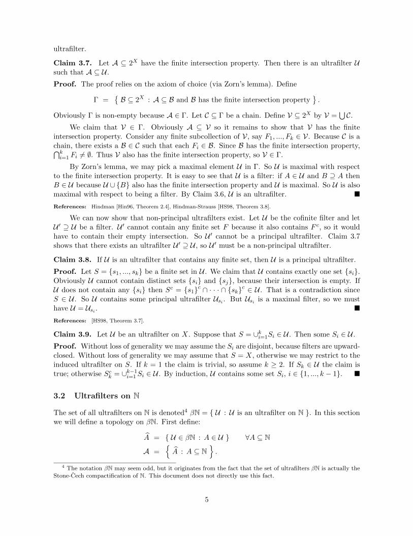
Claim 3.7. Let A ⊆ 2X have the finite intersection property. Then there is an ultrafilter Usuch that A ⊆ U .

Proof. The proof relies on the axiom of choice (via Zorn’s lemma). Define

Γ ={B ⊆ 2X : A ⊆ B and B has the finite intersection property

}.

Obviously Γ is non-empty because A ∈ Γ. Let C ⊆ Γ be a chain. Define V ⊆ 2X by V =⋃C.

We claim that V ∈ Γ. Obviously A ⊆ V so it remains to show that V has the finiteintersection property. Consider any finite subcollection of V, say F1, ..., Fk ∈ V. Because C is achain, there exists a B ∈ C such that each Fi ∈ B. Since B has the finite intersection property,⋂ki=1 Fi 6= ∅. Thus V also has the finite intersection property, so V ∈ Γ.

By Zorn’s lemma, we may pick a maximal element U in Γ. So U is maximal with respectto the finite intersection property. It is easy to see that U is a filter: if A ∈ U and B ⊇ A thenB ∈ U because U ∪ {B} also has the finite intersection property and U is maximal. So U is alsomaximal with respect to being a filter. By Claim 3.6, U is an ultrafilter. �

References: Hindman [Hin96, Theorem 2.4], Hindman-Strauss [HS98, Theorem 3.8].

We can now show that non-principal ultrafilters exist. Let U be the cofinite filter and letU ′ ⊇ U be a filter. U ′ cannot contain any finite set F because it also contains F c, so it wouldhave to contain their empty intersection. So U ′ cannot be a principal ultrafilter. Claim 3.7shows that there exists an ultrafilter U ′ ⊇ U , so U ′ must be a non-principal ultrafilter.

Claim 3.8. If U is an ultrafilter that contains any finite set, then U is a principal ultrafilter.

Proof. Let S = {s1, ..., sk} be a finite set in U . We claim that U contains exactly one set {si}.Obviously U cannot contain distinct sets {si} and {sj}, because their intersection is empty. IfU does not contain any {si} then Sc = {s1}c ∩ · · · ∩ {sk}c ∈ U . That is a contradiction sinceS ∈ U . So U contains some principal ultrafilter Usi . But Usi is a maximal filter, so we musthave U = Usi . �

References: [HS98, Theorem 3.7].

Claim 3.9. Let U be an ultrafilter on X. Suppose that S = ∪ki=1Si ∈ U . Then some Si ∈ U .

Proof. Without loss of generality we may assume the Si are disjoint, because filters are upward-closed. Without loss of generality we may assume that S = X, otherwise we may restrict to theinduced ultrafilter on S. If k = 1 the claim is trivial, so assume k ≥ 2. If Sk ∈ U the claim istrue; otherwise Sck = ∪k−1i=1 Si ∈ U . By induction, U contains some set Si, i ∈ {1, ..., k − 1}. �

3.2 Ultrafilters on N

The set of all ultrafilters on N is denoted4 βN = { U : U is an ultrafilter on N }. In this sectionwe will define a topology on βN. First define:

A = { U ∈ βN : A ∈ U } ∀A ⊆ N

A ={A : A ⊆ N

}.

4 The notation βN may seem odd, but it originates from the fact that the set of ultrafilters βN is actually theStone-Cech compactification of N. This document does not directly use this fact.

5

Claim 3.10. For every A,B ⊆ N, A ∩B = A ∩ B.

Proof. The proof is just a matter of understanding the definitions:

U ∈ A ∩ B ⇐⇒ A,B ∈ U ⇐⇒ A ∩B ∈ U ⇐⇒ U ∈ A ∩B.

�

References: Hindman [Hin96, Lemma 2.7(a)], Hindman-Strauss [HS98, Lemma 3.17(a)].

Claim 3.11. For every A ⊆ N, (βN) \ A = (Ac). Consequently, A is closed under complements;that is, the family of complements of members of A is A itself.

Proof. We omit the proof, which again follows directly from the definitions. �

References: Hindman [Hin96, Lemma 2.7(c)], Hindman-Strauss [HS98, Lemma 3.17(c)].

Claim 3.10 shows that A is closed under finite intersections. Obviously⋃A∈A A = βN, so

by Fact A.3 we may define the topology on βN to be all unions of members of A. The familyA is a base for the open sets of this topology. By Claim 3.11, the family of complements ofmembers of A is A itself so, by Fact A.5, A is also a base for the closed sets. This implies thatevery set A is clopen.

Claim 3.12. βN is compact.

Proof. Recall that A is a base for the closed sets. By Claim A.8, it suffices to show thatevery subcollection B ⊆ A with the finite intersection property has non-empty intersection. Let

S ={S ⊆ N : S ∈ B

}.

We claim that S has the finite intersection property. To see this, for any S1, ..., Sk ∈ S,there exists U ∈

⋂ki=1 Si (since B has the finite intersection property), so S1, ..., Sk ∈ U , which

implies⋂ki=1 Si ∈ U , and hence

⋂ki=1 Si is not empty.

Claim 3.7 implies that there is an ultrafilter U ⊇ S. This means that U ∈ S for all S ∈ S,i.e.,

⋂B is non-empty. �

References: Hindman [Hin96, Lemma 2.11], Hindman-Strauss [HS98, Theorem 3.18(a)].

Claim 3.13. The principal ultrafilters are dense in βN.

Proof. Since A is a base, it suffices to show that, for every A ⊆ N, A contains a principalultrafilter. For every i ∈ A, obviously A ∈ Ui, so Ui ∈ A. �

References: Hindman [Hin96, Lemma 2.10], Hindman-Strauss [HS98, Theorem 3.18(e)].

Claim 3.14. βN is Hausdorff.

Proof. Let U ,V ∈ βN be distinct. Fix any set A ∈ U \ V; then Ac ∈ V \ U . Then A and (Ac)

are disjoint open sets with U ∈ A and V ∈ (Ac). �

References: Hindman [Hin96, Lemma 2.8], Hindman-Strauss [HS98, Theorem 3.18(a)].

3.3 βN and limits of sequences

Let a = (a1, a2, ...) ∈ CN be a bounded sequence (i.e., a ∈ `∞). The sequence a might not havea limit. We will show that an ultrafilter U can be used to define a “U-limit”.

Definition 3.15. Let a ∈ CN and U ∈ βN. We say that a point x ∈ C is a U-limit of a if, forevery neighborhood S of x, we have { i : ai ∈ S } ∈ U .

6

Claim 3.16. If a ∈ CN has a U-limit, it is unique.

Proof. Let x and x′ be distinct points in C. Let S and S′ be disjoint neighborhoods of x andx′ respectively. Then the sets { i : ai ∈ S } and { i : ai ∈ S′ } are disjoint, so they cannot bothbelong to U . So x and x′ cannot both be U-limits. �

References: Hindman [Hin96, Theorem 2.16(a)], Hindman-Strauss [HS98, Theorem 3.48(a)].

So, if a ∈ CN has a U-limit, we may denote it by U-lim a.

Claim 3.17. Let a ∈ CN and let U ∈ βN be the principal ultrafilter Uj for some j ∈ N. ThenU-lim a = aj .

Proof. Fix any neighborhood S of aj and let A = { i : ai ∈ S }. Obviously j ∈ A so A ∈ U .Thus aj is a U-limit of a. �

Claim 3.18. If a ∈ `∞ then U-lim a exists.

Proof. Let X ⊆ C be a compact set such that each ai ∈ X. If U-lim a does not exist then, forevery x ∈ X, there must exist an open neighborhood Sx with { i : ai ∈ Sx } 6∈ U . Then X ⊆⋃x∈X Sx, so there exists a finite F ⊆ X with X ⊆

⋃x∈F Sx. Then N =

⋃x∈F { i : ai ∈ Sx }.

Claim 3.9 shows that some x has { i : ai ∈ Sx } ∈ U , which is a contradiction. �

References: Hindman [Hin96, Theorem 2.16(b)], Hindman-Strauss [HS98, Theorem 3.48(b)].

Claim 3.19. Let U be an ultrafilter and let I ∈ U . Let a ∈ CN and suppose that U-lima exists.Define A = { ai : i ∈ I }. Then U-lim a ∈ A, the closure of A.

Proof. Suppose not. Then X := (A)c is a neighborhood of U-lim a, so { i : ai ∈ X } ∈ U .But { i : ai ∈ X } is disjoint from I, so their empty intersection must also be in U , which is acontradiction. �

Claim 3.20. The U-lim operator is linear. That is, for a, b ∈ CN and c, d ∈ C, we havec · U-lim a+ d · U-lim b = U-lim (ca+ db) whenever the left-hand side exists.

Proof. Define la = U-lim a and lb = U-lim b. For any ε > 0,

{ i : |cai − c · la| < |c|ε } = { i : |ai − la| < ε } ∈ U{ i : |dbi − d · lb| < |d|ε } = { i : |bi − lb| < ε } ∈ U

Their intersection is also in U , and hence { i : |(cai + dbi)− (c · la + d · lb)| < 2ε } ∈ U . Takingε ↓ 0, we see that c · la + d · lb is a U-limit of ca+ db. �

References: Tricki.

Claim 3.21. Let a, b ∈ CN and let ab be their pointwise product, i.e., (ab)i = ai · bi. Then(U-lim a

)·(U-lim b

)= U-lim (ab) whenever the left-hand side exists.

Proof. The proof is similar to the previous proof, and the usual argument that limits aremultiplicative (e.g., Rudin [Rud76, Theorem 3.3]). �

Claim 3.22. Let a ∈ CN and let a∗ be its pointwise conjugate, i.e., (a∗)i = (ai)∗. Then(

U-lim a)∗

= U-lim (a∗) whenever the left-hand side exists.

Proof. The proof is easy and omitted. �

As in Example B.2, define C(βN) to be the Banach space of continuous, complex-valuedfunctions on βN with the supremum norm ‖f‖u = sup { |f(U)| : U ∈ βN }. Since βN is compact,all such functions are bounded (by Fact A.10).

7

Claim 3.23. The Banach spaces `∞ and C(βN) are isometrically isomorphic.

Proof. For any continuous function f : βN→ C, define af ∈ CN by afi = f(Ui). We claim thataf ∈ `∞. Since βN is compact and f is continuous, Fact A.10 shows that f(βN) is a compact

subset of C. Thus{afi : i ∈ N

}= { f(Ui) : i ∈ N } is bounded.

Conversely, for any a ∈ `∞, define fa : βN→ C by fa(U) = U-lim a. We now argue that fais continuous. Let S be a neighborhood of fa(U). Let S′ ⊆ S be a closed neighborhood of fa(U).Then I := { i : ai ∈ S′ } ∈ U . Since I is open in the topology of βN, it is a neighborhood of U .We claim that fa(V) ∈ S′ for all V ∈ I. Define A := { ai : i ∈ I } ⊆ S′. Since I ∈ V, we applyClaim 3.19 to obtain V-lim a ∈ A. Since S′ is closed, A ⊆ S′, so fa(V) ∈ S′. Thus fa(I) ⊆ S.By Fact A.11, fa is continuous.

Next we claim that the maps a 7→ fa and f 7→ af are mutually inverse. It is easy tosee that afa = a for every a ∈ `∞. Next we claim that, we must have faf = f for everyf ∈ C(βN). To see this, first note that f and faf agree on the principal ultrafilters, because

faf (Ui) = Ui-lim af = afi = f(Ui), by Claim 3.17. By Claim 3.13, the principal ultrafilters are adense subset of βN. Thus faf and f are continuous functions that agree on a dense set of thedomain, so by Fact A.12 they must be equal.

For any a ∈ `∞ we have

‖a‖∞ = supi∈N|ai| = sup

i∈N|fa(Ui)| = sup

U∈βN|fa(U)| = ‖fa‖u ,

where the third equality holds since the principal ultrafilters are dense in N (Claim 3.13) and fais continuous. �

4 Ultrafilters on N and functionals on D(`2)

The main goal of this section is to understand the pure states on D(`2). To do so, we will usethe fact, established in Section 3, that D(`2) and C(βN) are isometrically isomorphic. It turnsout that the pure states on D(`2) are closely related to ultrafilters.

Before discussing states on D(`2), we must first observe that this is a C∗-algebra. One cansee this directly, but instead let us recall that Claim 3.12 shows that βN is compact and Haus-dorff, so Example C.6 shows that C(βN) is a C∗-algebra. Thus, a consequence of Example B.14and Claim 3.23 is:

Corollary 4.1. The C∗-algebras D(`2) and C(βN) are isometrically isomorphic.

Let diag : D(`2) → `∞ be the canonical isometry, as described in Example B.14. For anyU ∈ βN, define the functional fU : D(`2)→ C by

fU (D) = U-lim (diagD). (4.1)

Theorem 4.2. The pure states on D(`2) are precisely the functionals of the form fU for U ∈ βN.

References: Tanbay [Tan91, pp. 707].

Recall the two-dimensional example in Section 2 in which the only pure states were f1(d1, d2) =d1 and f2(d1, d2) = d2. This is consistent with Theorem 4.2 as Claim 3.8 shows that the onlyultrafilters on {1, 2} are the principal ultrafilters U1 = {{1} , {1, 2}} and U2 = {{2} , {1, 2}}.

8

As a step towards Theorem 4.2, we start with a smaller theorem which shows that, givenany pure state, we can extract an ultrafilter. Recalling Definition B.15, the projections in D(`2)are { PA : A ⊆ N } where

〈 PAei, ei 〉 =

{1 if i ∈ A0 otherwise

.

Theorem 4.3. Given any pure state f : D(`2)→ C, define U = { A ⊆ N : f(PA) = 1 }. ThenU is an ultrafilter.

In order to prove these theorems, we require the following characterization of pure stateson D(`2).

Claim 4.4. A (non-zero) linear functional on D(`2) is a pure state if and only if it is multi-plicative.

Proof. Directly from Corollary 4.1, Claim 3.14, Claim 3.12 and Fact C.23. �

Claim 4.5. Let f : D(`2) → C be a pure state and let P ∈ D(`2) be a projection. Thenf(P ) ∈ {0, 1}.Proof. By Claim 4.4, f is multiplicative. So f(P ) = f(P 2) = f(P )2, implying f(P ) ∈ {0, 1}.�

Proof (of Theorem 4.3).

• N ∈ U because f(PN) = f(1) = 1.• ∅ 6∈ U because P∅ = 0 and f(0) = 0 by linearity.• Suppose A ∈ U and A ⊆ B. So f(PA) = 1. Note that PB = PA + PB\A. By Claim 4.5,

linearity and positivity of f , 1 ≥ f(PB) = f(PA) + f(PB\A) ≥ f(PA) = 1, so f(PB) = 1.• Let A ⊆ N be arbitrary. Then 1 = f(I) = f(PA) + f(PAc). By Claim 4.5, exactly one off(PA) and f(PAc) is 1, so exactly one of A or Ac is in U .

• Suppose A ∈ U and B ∈ U . Then A ∪ B ∈ U , so f(PA) = f(PB) = f(PA∪B) = 1. Bylinearity of f ,

1 = f(PA) = f(PA\B) + f(PA∩B)

1 = f(PB) = f(PB\A) + f(PA∩B)

1 = f(PA∪B) = f(PA\B) + f(PB\A) + f(PA∩B)

This is only possible if f(PA∩B) = 1, because f(PA\B), f(PB\A), f(PA∩B) ∈ {0, 1} byClaim 4.5. So A ∩B ∈ U .

�

Claim 4.6. For any U ∈ βN, fU is a *-homomorphism (cf. Definition C.11).

Proof. Fix U and define g : `∞ → C by a 7→ U-lim a. The function g

• Is homogeneous: Claim 3.20 implies that g(ca) = c · g(a) for c ∈ C and a ∈ `∞.• Is additive: Claim 3.20 implies that g(a+ b) = g(a) + g(b) for all a, b ∈ `∞.• Is multiplicative: Claim 3.21 implies that g(ab) = g(a) · g(b) for all a, b ∈ `∞.• Is unital : Claim 3.19 implies that g(1) = 1.• Commutes with conjugation: Claim 3.22 implies that g(a∗) = g(a)∗ for all a ∈ `∞.

fU has the same properties because fU (D) = g(diagD). �

Proof (of Theorem 4.2). The fact that fU is a pure state on D(`2) follows from Claim 4.4 and

9

Claim 4.6. Next, given any pure state on D(`2), define U as in Theorem 4.3. We claim thatf = fU , i.e., for every D ∈ D(`2), we have f(D) = U-lim diagD. It suffices to consider thecase that D is a projection, by Fact B.16 and the fact that f is linear. Thus, assume D = PAand d = diagD ∈ {0, 1}N has di = 1 iff i ∈ A. If f(PA) = 1 then A ∈ U , so U-lim d = 1 byClaim 3.19. Conversely, if f(PA) = 0 then Ac ∈ U , so U-lim d = 0 by Claim 3.19. �

4.1 Statement of the Kadison-Singer Problem

Let f : D(`2) → C be a linear functional. A linear functional g : B(`2) → C is called anextension of f to B(`2) if g(D) = f(D) for all D ∈ D(`2). Additionally, if f and g are bothstates then then g is called a state extension of f . Similarly, if f and g are both pure statesthen g is called a pure state extension of f .

The Kadison-Singer problem is:

Problem 1.1. Is it true that, for every pure state f : D(`2) → C on D(`2), there is a uniquefunctional g : B(`2)→ C that is a state extension of f?

Claim 4.8 clarifies the problem somewhat. First we require a definition

Definition 4.7. For H ∈ B(`2), let E(H) ∈ D(`2) be the “diagonal of H”, i.e., 〈 E(H)ei, ej 〉equals 〈 Hei, ei 〉 if i = j and equals zero otherwise. This is also called the conditionalexpectation of H. Obviously E : B(`2)→ D(`2) is linear.

Claim 4.8.

(1): Every state on D(`2) has a state extension to B(`2). More precisely, if f : D(`2)→ Cbe a state, define g : B(`2)→ C by g(H) = f(E(H)). Then g is a state.

(2): Every pure state on D(`2) has a pure state extension to B(`2).

(3): Let f be a pure state on D(`2). If g is the unique pure state extension of f to B(`2),then g is also the unique state extension of f to B(`2).

References: Dixmier [Dix77, Lemma 2.10.1]. For (1), see also Kadison-Ringrose [KR83, Theorem 4.3.13(ii)], Fact C.20,

Lemma 5.6. For (2) and (3), see Kadison-Ringrose [KR83, Theorem 4.3.13(iv)].

Proof. We prove only (1). Clearly g(1) = f(E(1)) = f(1) = 1. Clearly g is linear because it isthe composition of linear functions. It remains to check positivity. If H ∈ B(`2) is positive then〈Hei, ei 〉 ≥ 0 for all i, as in Example C.10. Thus E(H) is also positive. Since f is positive, wehave g(H) = f(E(H)) ≥ 0. �

Statements (2) and (3) together show that Problem 1.1 is equivalent after replacing thewords “state extension” with “pure state extension”.

5 Reduction to the paving problem

In this section we show that the Kadison-Singer conjecture is equivalent to Anderson’s pavingconjecture. The argument is copied nearly verbatim from Paulsen and Raghupathi [PR08].

10

5.1 Generic results about C∗-algebras

Fix real numbers a, b with 0 < a < 1 < b. Let B be a unital C∗-algebra. Define

P[a, b] = { P ∈ B : aI � P � bI } .

Note that every element of P[a, b] is self-adjoint and positive. The set P[a, b] is closed andconvex.

Claim 5.1 ([PR08, Theorem 2.1]). Let B be a unital C∗-algebra and let si : B → C (fori = 1, 2) be states. The following are equivalent:

1: s1 = s2,

2: s1(p)s2(p−1) ≥ 1 for every positive, invertible p ∈ B,

3: s1(p)s2(p−1) ≥ 1 for every p ∈ P[a, b].

Proof. (1) ⇒ (2): Suppose that s : B → C is a state and that q ∈ B is positive and invertible.For any t ∈ R, the operator tq + q−1 is self-adjoint, so (tq + q−1)2 is positive, so

0 ≤ s((tq + q−1)2

)= t2s(q2) + 2t+ s(q−2).

Since this quadratic function of t is non-negative, its discriminant 4 − 4s(q2)s(q−2) must benon-positive. Thus s(q2)s(q−2) ≥ 1. This proves (2) by substituting any p ∈ P[a, b] for q2 = pand setting s = s1 = s2.

(2) ⇒ (3): Trivial.

(3) ⇒ (1): Let h ∈ B be self-adjoint. Define the function f(t) = s1(eth)s2(e

−th). For real tin a sufficiently small neighborhood of 0, we have eth ∈ P[a, b], so (3) implies f(t) ≥ 1 in thatneighborhood. But f(0) = 1, so 0 is a minimizer and f ′(0) = 0. One can show that

df

dt= s1

(heth

)s2(e

−th) + s2(−he−th

)s1(e

th)

Thus 0 = f ′(0) = s1(h) − s2(h). That is, s1(h) = s2(h) for all self-adjoint h, so s1 = s2 byClaim C.13. �

Let S ⊆ B be an operator system (see Definition C.12). For any state s : S → C and anyself-adjoint p ∈ B, define

`s(p) = sup { s(q) : p � q ∈ S }us(p) = inf { s(q) : p � q ∈ S }

Here q is implicitly assumed to be self-adjoint, so s(q) ∈ R. Clearly `s(p) ≤ us(p), since forevery q � p � q′, we have f(q) ≤ f(q′) by Claim C.15.

Claim 5.2. Let s′ : B → C be any state extension of the state s : S → C. Then, for everyself-adjoint p ∈ B, we have

`s(p) ≤ s′(p) ≤ us(p).

Proof. Since s′ is a state, for any q ∈ S with q � p we have s′(q) ≤ s′(p) by Claim C.15. Sinces′ extends s we have s′(q) = s(q). Thus s(q) ≤ s′(p). Taking the supremum over q proves thefirst inequality. The other inequality is similar. �

11

Claim 5.3. For any p ∈ S we have `s(p) = us(p) = s(p).

Proof. Taking q = p in the definition of `s and us, we see that `s(p) ≥ s(p) and us(p) ≤ s(p).The reverse direction `s(p) ≤ us(p) was noted above. �

Claim 5.4. For any p ∈ B and q ∈ S we have

`s(p+ q) = `s(p) + `s(q) and us(p+ q) = us(p) + us(q).

Claim 5.5. `s(p) = −us(−p).Next we require Krein’s extension theorem.

Lemma 5.6. Let s : S → C be a state and let p ∈ B be self-adjoint. For every t with`s(p) ≤ t ≤ us(p) there exists a state st : B → C that extends s and satisfies st(p) = t.

References: Kadison-Ringrose [KR83, Theorem 4.3.13(ii)], Krein [Kre40], Paulsen-Raghupathi [PR08, Proposition 2.2].

Proof. If p ∈ S then `s(p) = us(p) so there is nothing to prove, so assume p 6∈ S. Define theoperator system T = { a+ λp : a ∈ S, λ ∈ C }. Fix t satisfying the condition of the claim, anddefine the linear functional f : T → C by f(a+ λp) = s(a) + λt.

Consider any positive operator a+ λp ∈ T . Positivity implies that it is self-adjoint, whichin turn implies that a is self-adjoint (since p is). Furthermore, λ must be real.

We claim that f(a+ λp) ≥ 0, i.e., f is a positive linear functional on T .

Case 1: λ > 0. Then p � −a/λ. Thus, by definition of `s(p), we have s(−a/λ) ≤ `s(p) ≤ t, wherethe second inequality is by our hypothesis on t. Thus f(a+λp) = s(a)+λt ≥ s(a)+λs(−a/λ) = 0.

Case 2: λ < 0. The argument is similar.

This proves the claim. Furthermore, 1 ∈ S so f(1) = s(1) = 1, and so f is a state on T .By Fact C.20, f can be extended to a state on B. �

Theorem 5.7 ([PR08, Theorem 2.3]). Let B be a unital C∗-algebra, let S ⊆ B be an operatorsystem and let s : S → C be a state. The following are equivalent.

1: s extends uniquely to a state on B,

2: for every self-adjoint p ∈ B, `s(p) = us(p),

3: for every positive, invertible p ∈ B, `s(p)`s(p−1) ≥ 1,

4: for every p ∈ P[a, b], `s(p)`s(p−1) ≥ 1.

Proof. (1) ⇔ (2): This follows directly from Claim 5.2 and Lemma 5.6. See also [KR83,Theorem 4.3.13(iii)].

(1) and (2) ⇒ (3): Let s1 be the unique state extension of s. Then, for every p ∈ B,s1(p) = `s(p). So `s(p)`s(p

−1) = s1(p)s1(p−1) ≥ 1, by Claim 5.1.

(3) ⇒ (4): This is trivial.

(4)⇒ (1): Suppose s1 and s2 are two state extensions of s. Claim 5.2 yields s1(p)s2(p−1) ≥

`s(p)`s(p−1) ≥ 1 for any p ∈ P[a, b], by condition (4). By Claim 5.1, s1 = s2. �

5.2 The Kadison-Singer problem

First we need a simple fact about Hilbert spaces.

12

Lemma 5.8. Let H and K be Hilbert spaces and let H =(A BB∗ C

)∈ B(H⊕K) be self-adjoint

with A positive and invertible. Then there exists δ > 0 such that H + δPK � 0, where PKdenotes the orthogonal projection onto K.

Proof. Let X = A−1/2B. Then, by Cauchy-Schwarz,⟨( A BB∗ C + δIK

)(hk

),

(hk

)⟩= 〈Ah, h 〉+ 〈A1/2Xk, h 〉+ 〈X∗A1/2h, k 〉+ 〈 Ck, k 〉+ δ ‖k‖2

≥∥∥∥A1/2h

∥∥∥2 − 2 ‖Xk‖∥∥∥A1/2h

∥∥∥− ‖C‖ ‖k‖2 + δ ‖k‖2

≥(∥∥∥A1/2h

∥∥∥− ‖Xk‖)2 + (δ − ‖C‖ − ‖X‖2) ‖k‖2 .

This is non-negative if δ ≥ ‖C‖+ ‖X‖2. �

This next lemma contains the heart of the proof: the connection between unique extensionsand matrix pavings.

Lemma 5.9. Let U ∈ βN and let fU : D(`2) → C be the corresponding pure state (defined in(4.1)). Fix any self-adjoint H ∈ B(`2). For t ∈ R, the following two conditions are equivalent:

1: `fU (H) = ufU (H) = t,

2: ∀ε > 0, ∃A ∈ U such that (t− ε)PA � PAHPA � (t+ ε)PA.

Proof. (2) ⇒ (1): Fix ε and A satisfying (2). Let f : B(`2) → C be any state extensionof fU . Then f(PA) = fU (PA) = 1 and f(PAc) = fU (PAc) = 0, as argued in the proof ofTheorem 4.2. Then f(PAcH) = 0 by Corollary C.19. Since I = PA + PAc , linearity impliesf(H) = f(PAH) + f(PAcH) = f(PAH). Repeating this argument, f(PAHPA) = f(H). Thus,by (2) and Claim C.15, we have t−ε ≤ f(H) ≤ t+ε. Taking ε ↓ 0, we have shown that f(H) = tfor every state extension f of fU . By Lemma 5.6, we must have `fU (H) = ufU (H) = t.

(1) ⇒ (2): Fix any ε > 0. There exist self-adjoint D1, D2 ∈ D(`2) with D1 � H � D2 andt− ε/2 ≤ fU (D1) ≤ fU (D2) ≤ t+ ε/2. (Since Di is self-adjoint, fU (Di) is real, by Claim C.17.)

Recall Definition 3.15. For j ∈ {1, 2}, since fU (Dj) = U-lim (diagDj) we have Aj :={ i : |(diagDj)i − fU (Dj)| < ε/2 } ∈ U . Then A := A1 ∩A2 ∈ U . So, for all i ∈ A,

(diagD1)i > t− ε and (diagD2)i < t+ ε.

ThusPA(D1 − (t− ε)I

)PA � 0 and PA

((t+ ε)I −D2

)PA � 0.

Apply Lemma 5.8 to D1 − (t − ε)I where H is the subspace corresponding to A and K = H⊥.(We only apply the lemma to this diagonal operator.) Then there exists δ1 > 0 such thatD1−(t−ε)I+δ1PAc � 0. Rearranging and multiplying by PA on both sides, PAD1PA � (t−ε)PA.A similar argument shows PAHPA � (t+ ε)PA. �

Recall from Definition 4.7 that E(H) is the “diagonal” of H.

Theorem 5.10. Let U ∈ βN and let fU : D(`2) → C be the corresponding pure state. Thefollowing are equivalent:

1: fU extends uniquely to a state on B(`2).

2: for every self-adjoint H ∈ B(`2) with E(H) = 0, we have `fU (H) = 0.

13

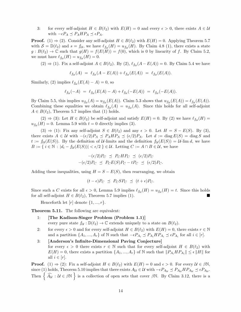
3: for every self-adjoint H ∈ B(`2) with E(H) = 0 and every ε > 0, there exists A ∈ Uwith −εPA � PAHPA � εPA.

Proof. (1)⇒ (2). Consider any self-adjoint H ∈ B(`2) with E(H) = 0. Applying Theorem 5.7with S = D(`2) and s = fU , we have `fU (H) = ufU (H). By Claim 4.8 (1), there exists a stateg : B(`2) → C such that g(H) = f(E(H)) = f(0), which is 0 by linearity of f . By Claim 5.2,we must have `fU (H) = ufU (H) = 0.

(2) ⇒ (1). Fix a self-adjoint A ∈ B(`2). By (2), `fU (A−E(A)) = 0. By Claim 5.4 we have

`fU (A) = `fU (A− E(A)) + `fU (E(A)) = `fU (E(A)).

Similarly, (2) implies `fU (E(A)−A) = 0, so

`fU (−A) = `fU (E(A)−A) + `fU (−E(A)) = `fU (−E(A)).

By Claim 5.5, this implies ufU (A) = ufU (E(A)). Claim 5.3 shows that ufU (E(A)) = `fU (E(A)).Combining these equalities we obtain `fU (A) = ufU (A). Since this holds for all self-adjointA ∈ B(`2), Theorem 5.7 implies that (1) holds.

(2) ⇒ (3): Let H ∈ B(`2) be self-adjoint and satisfy E(H) = 0. By (2) we have `fU (H) =ufU (H) = 0. Lemma 5.9 with t = 0 directly implies (3).

(3) ⇒ (1): Fix any self-adjoint S ∈ B(`2) and any ε > 0. Let H = S − E(S). By (3),there exists A ∈ U with −(ε/2)PA � PAHPA � (ε/2)PA. Let d := diagE(S) = diagS andt := fU (E(S)). By the definition of U-limits and the definition fU (E(S)) = U-lim d, we haveB := { i ∈ N : |di − fU (E(S))| < ε/2 } ∈ U . Letting C := A ∩B ∈ U , we have

−(ε/2)PC � PCHPC � (ε/2)PC

−(ε/2)PC � PCE(S)PC − tPC � (ε/2)PC .

Adding these inequalities, using H = S − E(S), then rearranging, we obtain

(t− ε)PC � PCSPC � (t+ ε)PC .

Since such a C exists for all ε > 0, Lemma 5.9 implies `fU (H) = ufU (H) = t. Since this holdsfor all self-adjoint H ∈ B(`2), Theorem 5.7 implies (1). �

Henceforth let [r] denote {1, ..., r}.

Theorem 5.11. The following are equivalent:

1: [The Kadison-Singer Problem (Problem 1.1)]every pure state fU : D(`2)→ C extends uniquely to a state on B(`2).

2: for every ε > 0 and for every self-adjoint H ∈ B(`2) with E(H) = 0, there exists r ∈ Nand a partition {A1, ..., Ar} of N such that −εPAi � PAiHPAi � εPAi for all i ∈ [r].

3: [Anderson’s Infinite-Dimensional Paving Conjecture]for every ε > 0 there exists r ∈ N such that for every self-adjoint H ∈ B(`2) withE(H) = 0, there exists a partition {A1, ..., Ar} of N such that ‖PAiHPAi‖ ≤ ε ‖H‖ forall i ∈ [r].

Proof. (1) ⇒ (2): Fix a self-adjoint H ∈ B(`2) with E(H) = 0 and ε > 0. For every U ∈ βN,since (1) holds, Theorem 5.10 implies that there exists AU ∈ U with−εPAU � PAUHPAU � εPAU .

Then{AU : U ∈ βN

}is a collection of open sets that cover βN. By Claim 3.12, there is a

14

finite subcollection{A1, ..., Ak

}that covers βN and satisfies −εPAi � PAiHPAi � εPAi for all

i.

To establish (2), we first note that⋃ki=1Ai = N. Indeed, for any j ∈ (

⋃ki=1Ai)

c, the

principal ultrafilter Uj cannot contain any Ai, so Uj 6∈⋃ki=1 Ai, which is a contradiction. So

{A1, ..., Ak} is a cover of N, but it might not be a partition because the sets need not be disjoint.Nevertheless, the partition of N obtained by intersecting those Ai’s in all possible ways satisfies(2) with r ≤ 2k.

(2) ⇒ (1): Fix an ultrafilter U ∈ βN, a self-adjoint H ∈ B(`2) with E(H) = 0, and ε > 0.By (2), there exists a partition {A1, ..., Ar} of N such that −εPAi � PAiHPAi � εPAi for all i.By Claim 3.9, some Ai ∈ U . Since this holds for all H and all ε, Theorem 5.10 implies that fUextends uniquely to a state on B(`2). Since U is arbitrary, this implies (1).

(3) ⇒ (2): Trivial.

(2) ⇒ (3): We prove the contrapositive. Suppose (3) does not hold. That is, there existsan ε > 0 such that for every r ∈ N, there exists a self-adjoint Hr ∈ B(`2) with E(Hr) = 0 suchthat no partition {A1, ..., Ar} of N satisfies ‖PAiHrPAi‖ ≤ ε ‖Hr‖ for all i. By rescaling, we mayassume that ‖Hr‖ = 1. Let H = H1 ⊕H2 ⊕H3 ⊕ · · ·. Then H is self-adjoint, E(H) = 0 and‖H‖ = 1, so H ∈ B(`2). Suppose (2) holds. Then there exists r ∈ N and a partition {A1, ..., Ar}satisfying −εPAi � PAiHPAi � εPAi for all i. In particular, restricting to the rth part of thedirect sum, −εPAi � PAiHrPAi � εPAi for all i. Equivalently, ‖PAiHrPAi‖ ≤ ε ‖Hr‖ for alli = 1, ..., r. This is a contradiction, so (2) cannot hold. �

6 Reduction to finite dimensional paving

Theorem 6.1. The following are equivalent:

1: [Anderson’s Infinite-Dimensional Paving Conjecture]for every ε > 0 there exists r ∈ N such that for every self-adjoint H ∈ B(`2) withE(H) = 0, there exists a partition {A1, ..., Ar} of N such that ‖PAiHPAi‖ ≤ ε ‖H‖ forall i ∈ [r].

2: [Anderson’s Finite-Dimensional Paving Conjecture]for every ε > 0 there exists r ∈ N such that for every n ∈ N and every self-adjointoperator H on `n2 with E(H) = 0, there exists a partition {A1, ..., Ar} of [n] such that‖PAiHPAi‖ ≤ ε ‖H‖ for all i ∈ [r].

References: Tanbay [Tan91, Proposition 1.2], Casazza et al. [CFTW06, Theorem 2.3], Halpern et al. [HKW87, Theorem

2.3].

First we need a technical claim.

Claim 6.2 ([CFTW06, Proposition 2.2]). Suppose that An = {An1 , ..., Anr } is a partition of [n],for each n ≥ 1. Then there exists a partition B = {B1, ..., Br} of N such that, for every j ∈ [r]and every ` ∈ N, there exists nj,` ∈ N such that the ` smallest elements of Bj are all containedin A

nj,`j .

Proof. We construct a sequence of integers 1 ≤ k1 ≤ k2 ≤ · · · satisfying ki ≥ i and satisfyingthe following property. For each m ≥ 1, let jm ∈ [r] be the index such that m ∈ Akmjm ; then

m ∈ Akpjm for all p ≥ m.

15

Given the sequence of ki’s, define Bj = { m : jm = j }. It is obvious that {B1, ..., Br} is apartition of N. Now fix j ∈ [r], let I be the ` smallest elements of Bj , and let p be the largest

element of I. For any m ∈ I we have jm = j, so m ∈ Akmj and m ∈ Akpj . Taking n = kp, wehave I ⊆ Anj .

We construct the sequence of ki’s as follows. Let S0 = N. Since S0 is infinite, there mustexist a j1 ∈ [r] and an infinite subset S1 ⊆ S0 such that 1 is contained in every set Anj1 for alln ∈ S1. Since S1 is infinite, there must exist a j2 ∈ [r] and an infinite subset S2 ⊆ S1 such that2 is contained in every set Anj2 for all n ∈ S2. Inductively define the chain S0 ⊇ S1 ⊇ S2 ⊇ · · ·.

Now define km to be the smallest element of Sm. Clearly km ≥ m. For every m ≥ 1 we havem ∈ Anjm for all n ∈ Sm; in particular m ∈ Akmjm . Furthermore, for each p ≥ m, kp ∈ Sp ⊆ Sm,

so m ∈ Akpjm , as required. �

Proof (of Theorem 6.1). (1) ⇒ (2): Trivial.

(2) ⇒ (1): Fix ε > 0 and let r be the integer whose existence is guaranteed by (2). Fixa self-adjoint H ∈ B(`2) with E(H) = 0. For every n ≥ 1, let Tn be the n × n matrix with(Tn)i,j = 〈Tei, ej 〉. Clearly ‖Tn‖ ≤ ‖T‖. By (2), there exists a partition An = {A1, ..., A1} of [n]such that ‖PAiTnPAi‖ ≤ (ε/2) ‖Tn‖ for all i ∈ [r]. Given these partitions A1,A2, ..., Claim 6.2produces a partition {B1, ..., Br} of N and integers nj,`.

Fix j ∈ [r] and ` ∈ N. Let I` be the ` smallest elements of Aj and let p be the largestelement of I`. As ‖PI`TPI`‖ →

∥∥PAjTPAj∥∥ monotonically, for sufficiently large ` we have∥∥PAjTPAj∥∥ ≤ 2∥∥PIjTPIj∥∥

= 2

∥∥∥∥PIjPAnj,`jTP

Anj,`j

PIj

∥∥∥∥≤ 2

∥∥∥∥PAnj,`jTP

Anj,`j

∥∥∥∥≤ 2(ε/2) ‖Tn‖≤ ε ‖T‖ ,

as required. �

6.1 Finite-dimensional paving conjectures

Let Cn×n be the set of complex n × n matrices. Recall that E(A) is the matrix containingthe diagonal entries of A (Definition 4.7), and PAi is the diagonal projection onto the set Ai(Definition B.15).

Theorem 6.3. The following are equivalent:

1: the Kadison-Singer problem has a positive solution,

2: ∀ε > 0, ∃r ∈ N, ∀n ∈ N and for every self-adjoint matrix A ∈ Cn×n with E(A) = 0,there exists a partition {A1, ..., Ar} of [n] such that ‖PAiAPAi‖ ≤ ε ‖A‖ ∀i ∈ [r].

3: ∀ε > 0, ∃r ∈ N, ∀n ∈ N and for every matrix A ∈ Cn×n with E(A) = 0, there exists apartition {A1, ..., Ar} of [n] such that ‖PAiAPAi‖ ≤ ε ‖A‖ ∀i ∈ [r].

4: ∀ε > 0, ∃r ∈ N, ∀n ∈ N and for every R ∈ Cn×n with R = R∗ = R−1 (i.e., a unitaryreflection matrix) and E(R) = 0, there exists a partition {A1, ..., Ar} of [n] such that‖PAiRPAi‖ ≤ ε ∀i ∈ [r].

16

5: ∀ε > 0, ∃r ∈ N, ∀n ∈ N and for every Q ∈ Cn×n with Q = Q∗ = Q2 (i.e., a complexorthogonal projection matrix) and E(Q) = I/2, there exists a partition {A1, ..., Ar} of[n] such that ‖PAiQPAi‖ ≤ (1 + ε)/2 ∀i ∈ [r].

6: ∀ε > 0, ∀ even N ≥ 2, ∃r ∈ N, ∀n ∈ N and for every Q ∈ Cn×n with Q = Q∗ =Q2 and Qi,i ∈ [0, 1/N ] for all i, there exists a partition {A1, ..., Ar} of [n] such that‖PAiQPAi‖ ≤ (1 + ε)/N ∀i ∈ [r].

7: ∀ε > 0, ∀ even N ≥ 2, ∃r ∈ N, ∀d ∈ N and for all v1, ..., vn ∈ Cd satisfying∑

j vjv∗j = I

and v∗j vj ≤ 1/N for all j ∈ [n], there exists a partition {A1, ..., Ar} of [n] such that we

have∥∥∥∑j∈Ai vjv

∗j

∥∥∥ ≤ (1 + ε)/N ∀i ∈ [r].

References: Portions are from Casazza et al. [CEKP07], Theorems 2 and 3.

Proof. (1) ⇔ (2): By Theorem 6.1.

(3) ⇒ (2): Trivial.

(2) ⇒ (3): Given A ∈ Cn×n we may write A = M + iN where M = (A + A∗)/2, N =i(A∗ − A)/2. Note that M and N are self-adjoint and ‖M‖ , ‖N‖ ≤ ‖A‖. If E(A) = 0 thenE(M) = E(N) = 0. Fix any ε > 0. By (2), there exist partitions {A1, ..., Ar} and {B1, ..., Br} of[n] such that ‖PAiMPAi‖ ≤ (ε/2) ‖M‖ and ‖PBiNPBi‖ ≤ (ε/2) ‖N‖. Then {Ci,j := Ai ∩Bj}i,jis a partition of [n] with∥∥PCi,jAPCi,j∥∥ ≤ ∥∥PCi,jMPCi,j

∥∥+∥∥PCi,jNPCi,j∥∥

≤ ‖PAiMPAi‖+∥∥PBjNPBj∥∥

≤ (ε/2)(‖M‖+ ‖N‖)≤ ε ‖A‖

(2) ⇒ (4): Trivial.

(4)⇒ (2): Let A ∈ Cn×n be self-adjoint with E(A) = 0. Since (2) is invariant under scalingA, we may assume ‖A‖ = 1. Then A2 � I, so we may define

R =

(A

√I −A2

√I −A2 −A

).

It is easy to check that R = R∗ and R2 = I, implying R = R∗ = R−1. All eigenvalues of R are±1, so ‖R‖ = 1 = ‖A‖. Furthermore, E(R) = 0. By (4), there exists a partition {A1, ..., Ar}of [2n] such that ‖PAiRPAi‖ ≤ ε for all i. Then {A1 ∩ [n], ..., Ar ∩ [n]} is a partition of [n] suchthat ‖PAiAPAi‖ ≤ ε for all i.

(4) ⇒ (5): Given Q with Q = Q∗ = Q2, let R = 2Q − I. Clearly R = R∗, and R2 =4Q2 − 4Q + I = I, implying R = R∗ = R−1. Furthermore if E(Q) = I/2 then E(R) = 0. By(4), there exists a partition {A1, ..., Ar} of [n] such that ‖PAiRPAi‖ ≤ ε for all i. Then

‖PAiQPAi‖ = ‖PAi(I +R)PAi‖ /2 ≤∥∥P 2

Ai

∥∥ /2 + ‖PAiRPAi‖ /2 ≤ (1 + ε)/2.

(5) ⇒ (4): Given R with R = R∗ = R−1 define Q = (I + R)/2. Clearly Q = Q∗ andQ2 = (I + 2R + R2)/4 = (I + R)/2 = Q. If additionally E(R) = 0 then E(Q) = I/2. By(5), there exists a partition {A1, ..., Ar} of [n] such that ‖PAiQPAi‖ ≤ (1 + ε)/2 ∀i ∈ [r]. Since0 � Q, we obtain

0 � PAiQPAi � (1 + ε)PAi/2.

17

Using R = 2Q− I, we get−PAi � PAiRPAi � εPAi .

This upper-bound is satisfactory but this lower-bound is not.

So apply the same argument to −R: define Q1 = (I − R)/2, so Q1 = Q∗1 = Q21 and

E(Q1) = I/2. By (5), there exists a partition {B1, ..., Br} of [n] such that

−PBi � PBi(−R)PBi � εPBi .

Define the partition {Ci,j := Ai ∩Bj}i,j of [n]. We have shown that:

PCi,jRPCi,j � PAiRPAi � εPAi

PCi,j (−R)PCi,j � PBi(−R)PBi � εPBi .

It follows that∥∥PCi,jRPCi,j∥∥ ≤ ε for all i, j.

(2)⇒ (6): By (2), for every ε > 0, there exists r ∈ N such that the following is true. GivenQ with Q = Q∗, 0 � Q � I and Qi,i ∈ [0, δ], let A = Q − E(Q). We have −δI � A � I, so‖A‖ ≤ 1. There exists a partition {A1, ..., Ar} of [n] such that ‖PAiAPAi‖ ≤ εδ for all i. Then

‖PAiQPAi‖ ≤ ‖PAiE(Q)PAi‖+ ‖PAiAPAi‖ ≤ δ + εδ.

(6) ⇒ (5): For any ε > 0 and even N ≥ 2, let r be such that (6) is true. Let Q ∈ Cn×nsatisfy Q = Q∗ = Q2 and E(Q) = I/2. Let J ∈ RN×N be the matrix of all ones. Letk = N/2 and let M ∈ Cnk×nk be the Kronecker product Q ⊗ J/k. It is easy to check thatM = M∗ = M2 and Mi,i = 1/2k = 1/N . By (6), there exists a partition {A1, ..., Ar} of [nk]such that ‖PAiMPAi‖ ≤ (1 + ε)/N ∀i ∈ [r]. Then∥∥PAi∩[n]QPAi∩[n]∥∥ ≤ k ‖PAiMPAi‖ ≤ k(1 + ε)/N ≤ (1 + ε)/2.

(7) ⇒ (6): For any ε > 0 and even N ≥ 2, let r be such that (7) is true. Let Q ∈ Cn×nsatisfy Q = Q∗ = Q2 and Qi,i ∈ [0, 1/N ] for all i. Let V be a d×n matrix with Q = V ∗V , whered is the rank of Q. Let vj be the jth column of V , so v∗j vj = Qj,j ≤ 1/N . By (7), there exists a

partition {A1, ..., Ar} of [n] such that, for all i ∈ [r], we have∥∥∥∑j∈Ai vjv

∗j

∥∥∥ ≤ (1 + ε)/N .

For any complex matrix M , the matrices MM∗ and M∗M have the same non-zero eigen-values. It follows that, for any A ⊆ [n],

‖PAQPA‖ = ‖PAV ∗V PA‖ = ‖V PAV ∗‖ =∥∥∥∑j∈Avjv

∗j

∥∥∥ . (6.1)

So, ‖PAiQPAi‖ ≤ (1 + ε)/N for all i ∈ [r]. This proves (6).

(6) ⇒ (7): For any ε > 0 and even N ≥ 2, let r be such that (6) is true. Let v1, ..., vn ∈ Cdsatisfy

∑j vjv

∗j = I and v∗j vj ≤ 1/N . Define the n × n matrix Q by Qi,j = v∗i vj . That is,

if V ∈ Cd×n is the matrix whose jth column is vj then Q = V ∗V . Clearly Q = Q∗, andQ2 = V ∗V V ∗V = V ∗V = Q. Furthermore, Qi,i ∈ [0, 1/N ] because Qi,i = v∗i vi. By (6), thereexists a partition {A1, ..., Ar} of [n] such that ‖PAiQPAi‖ ≤ (1 + ε)/N for all i ∈ [r]. By (6.1),this implies (7). �

18

6.2 Finite-dimensional paving conjectures with existential quantification

In this section we briefly observe that the conjectures of the previous section are equivalent underreplacing the universal quantification “∀ε > 0” with the existential quantification “∃α ∈ (0, 1)”.

Theorem 6.4. The following are equivalent:

1: the Kadison-Singer problem has a positive solution,

2: ∃α ∈ (0, 1), ∃r ∈ N, ∀n ∈ N and for every self-adjoint matrix A ∈ Cn×n with E(A) = 0,there exists a partition {A1, ..., Ar} of [n] such that ‖PAiAPAi‖ ≤ α ‖A‖ ∀i ∈ [r].

3: ∃α ∈ (0, 1), ∃r ∈ N, ∀n ∈ N and for every R ∈ Cn×n with R = R∗ = R−1 (i.e., aunitary reflection matrix) and E(R) = 0, there exists a partition {A1, ..., Ar} of [n]such that ‖PAiRPAi‖ ≤ α ∀i ∈ [r].

4: ∃α ∈ (0, 1), ∃r ∈ N, ∀n ∈ N and for every Q ∈ Cn×n with Q = Q∗ = Q2 (i.e., a complexorthogonal projection matrix) and E(Q) = I/2, there exists a partition {A1, ..., Ar} of[n] such that ‖PAiQPAi‖ ≤ (1 + α)/2 ∀i ∈ [r].

5: ∃α ∈ (0, 1), ∃ even N ≥ 2, ∃r ∈ N, ∀n ∈ N and for every Q ∈ Cn×n with Q = Q∗ =Q2 and Qi,i ∈ [0, 1/N ] for all i, there exists a partition {A1, ..., Ar} of [n] such that‖PAiQPAi‖ ≤ (1 + α)/N ∀i ∈ [r].

6: ∃α ∈ (0, 1), ∃ even N ≥ 2, ∃r ∈ N, ∀d ∈ N and for all v1, ..., vn ∈ Cd satisfying∑j vjv

∗j = I and v∗j vj ≤ 1/N for all j ∈ [n], there exists a partition {A1, ..., Ar} of [n]

such that we have∥∥∥∑j∈Ai vjv

∗j

∥∥∥ ≤ (1 + α)/N ∀i ∈ [r].

Proof. (1) ⇒ (2): Follows from Theorem 5.11 and Theorem 6.1.

(2) ⇒ (1): Let α ∈ (0, 1) and r ∈ N be such that (2) is true. Let M ∈ Cn×n be self-adjointwith E(M) = 0. Fix any ε > 0. By (2), there exists a partition A1 of [n] such that

‖PAMPA‖ ≤ α ‖M‖ ∀A ∈ A1.

Applying this argument separately to each matrix in { PAMPA : A ∈ A1 }, we obtain a partitionA2 of [n] such that

‖PAMPA‖ ≤ α2 ‖M‖ ∀A ∈ A2.

Repeating k := dlogα εe times, we obtain a partition Ak of [n] such that

‖PAMPA‖ ≤ ε ‖M‖ ∀A ∈ Ak.

This shows that Theorem 6.1(2) holds, which implies (1) by Theorem 5.11.

The remainder of the equivalences are similar to the proof of Theorem 6.3. �

7 Weaver’s conjecture

Building on work of Akemann and Anderson [AA91], Weaver [Wea04] states a conjecture thatappears to be weaker than Theorem 6.3 (7) (or Theorem 6.4 (6)), but is actually equivalent.

Conjecture 7.1 (Conjecture KSr). ∃α > 0, ∃N ≥ 2, ∀d ∈ N, and for all w1, ..., wn ∈ Cdsatisfying

∑j wjw

∗j � I and w∗jwj ≤ 1/N for all j ∈ [n], there exists a partition {A1, ..., Ar} of

[n] such that, for all i ∈ [r], we have∥∥∥∑j∈Ai wjw

∗j

∥∥∥ ≤ 1− α/N .

19

Theorem 7.2 ([Wea04, Theorem 1]). The following are equivalent:

1: the Kadison-Singer problem has a positive solution,

2: There exists r ≥ 2 such that Conjecture KSr is true.

Proof. (1) ⇒ (2): Directly from Theorem 6.3 (7).

(2) ⇒ (1): Weaver’s proof is based on results of Akemann and Anderson [AA91], whichrequire much deeper operator theory than we are able to discuss here. �

The recent breakthrough of Marcus, Spielman and Srivastava is as follows:

Theorem 7.3 (Corollary 1.3 in [MSS13]). Let u1, ..., um ∈ Cd satisfy∑

i uiu∗i = I and ‖ui‖22 ≤ δ

for all i. Then there exists a partition of {1, ...,m} into two sets S1 and S2 such that∥∥∥∥∥∥∑i∈Sj

uiu∗i

∥∥∥∥∥∥2

≤ (1 +√

2δ)2

2∀j ∈ {1, 2} . (7.1)

This directly implies Conjecture KS2, and therefore a positive solution to Problem 1.1.

Question 7.4. Does Theorem 7.3 imply a solution to the Kadison-Singer problem withoutusing KSr as an intermediate step? For example, does Theorem 7.3 directly imply any of thestatements in Theorem 6.3?

Acknowledgements

I am grateful to Joel Friedman for many useful discussions.

20

A Point-set Topology

We state some standard definitions and facts from point-set topology. Some references for thismaterial are Folland [Fol99, Ch. 4], Royden [Roy88, Ch. 8], or Wikipedia.

Definition A.1. Let X be any non-empty set. A topology T on X is a family of subsets ofX such that

• ∅, X ∈ T ,• T is closed under arbitrary unions, and• T is closed under finite intersections.

A pair (X, T ) is called a topological space if T is a topology on X. When T is apparentor need not be named, we simply say that X is a topological space. The members of T arecalled open sets. A set A ⊆ X is closed if Ac is open. A set that is both closed and open iscalled clopen. In every topological space X, both ∅ and X are clopen.

For any S ⊆ X, the interior of S, denoted int(S) is the union of all open sets containedin S. A neighborhood of x ∈ X is any set S such that x ∈ int(S). Equivalently, N is aneighborhood of x if N contains an open set that contains x.

Definition A.2. Let (X, T ) be a topological space. A family B ⊆ T is called a base for T (ora base for the open sets of T ) if, for every x ∈ X and every open set U containing x, thereexists V ∈ B with x ∈ V ⊆ U .

For any S ⊆ X, the closure of S, denoted S, is the intersection of all closed sets containingS. A set S ⊆ X is dense in X if its closure equals X. Equivalently, letting B be a base, S isdense if every non-empty B ∈ B has B ∩ S 6= ∅. A topological space is separable if it has acountable dense subset. For example, Rn is separable because Qn is a countable dense subset.

Fact A.3. Let X be a non-empty set and B ⊆ 2X . Suppose that⋃B = X and B is closed

under finite intersections. Let T ={ ⋃

α∈AEα : Eα ∈ B}

be the collection of all unions ofmembers of B. Then T is a topology and B is a base for T .

Definition A.4. Let (X, T ) be a topological space. A family F is called a base for theclosed sets for T if every closed set is an intersection of members of F .

Fact A.5. Let X be a topological space. A family F is a base for the closed sets if and only ifthe family of complements of members of F is a base for the open sets.

Definition A.6. Let (X, T ) be a topological space. Suppose that, for every collection{Tα}α∈A ⊆ T satisfying X =

⋃α∈A Tα, there exists a finite subcollection T1, ..., Tk satisfying

X =⋃ki=1 Ti. Then X is called compact.

Definition A.7. Let C be a collection of sets. Suppose that, for every finite subcollectionC1, ..., Ck ∈ C, we have

⋂ki=1Ci 6= ∅. Then we say that C has the finite intersection property.

Claim A.8. Let (X, T ) be a topological space and let F be a base for the closed sets. Thefollowing are equivalent.

(i): X is compact.

(ii): For every collection {Cα}α∈A of closed sets with the finite intersection property, wehave

⋂α∈ACα 6= ∅.

21

(iii): For every subcollection {Fβ}β∈B ⊆ F with the finite intersection property, we have⋂β∈B Fβ 6= ∅.

Proof. (i) ⇒ (ii): Let {Cα}α∈A be a collection of closed sets with the finite intersectionproperty. Define the collection D = {Dα}α∈A of open sets by Dα = Ccα. Then, for every finite

subcollection D1, ..., Dk ∈ D, we have⋃ki=1Di = (

⋂ki=1Ci)

c 6= (∅)c = X. By (i), we must haveX 6=

⋃α∈ADα, so

⋂α∈ACα 6= ∅.

(ii) ⇒ (iii): Trivial.

(iii) ⇒ (i): Let {Tα}α∈A ⊆ T satisfy X =⋃α∈A Tα. Then Cα := T cα is closed and

⋂α∈ACα = ∅.

Each Cα can be written Cα =⋂F∈Fα F for some subcollection Fα ⊆ F . So

⋂F∈∪α Fα F = ∅. By

(iii),⋃α Fα does not have the finite intersection property. That is, there exists sets F1, ..., Fk ∈⋃

α Fα with⋂ki=1 Fi = ∅. For i = 1, ..., k, choose αi ∈ A satisfying Cαi ⊆ Fi. Then

⋂ki=1Cαi = ∅

also, so⋃ki=1 Tαi = X. �

Definition A.9. Let X and Y be topological spaces. A function f : X → Y is continuous iff−1(V ) is open for every open V ⊆ Y .

Fact A.10. Let X and Y be topological spaces where X is compact. If f : X → Y is continuousthen f(X) is compact.

Fact A.11. f : X → Y is continuous if and only if, for every x ∈ X and for every neighborhoodV of f(x), there exists a neighborhood U of x such that f(U) ⊆ V .

A topology on X is Hausdorff if, for every distinct x, y ∈ X, there exist disjoint opensets Sx and Sy with x ∈ Sx and y ∈ Sy. For example, for finite n, the standard topology on Rnor Cn is Hausdorff.

Fact A.12. Let X and Y be topological spaces, where Y is Hausdorff. Let f, g : X → Y becontinuous functions that agree on a dense subset of X. Then f and g agree on all of X.

B Banach and Hilbert Spaces

We state some standard definitions and facts from functional analysis. Some references for thismaterial are Albiac and Kalton [AK06, Ch. 1, 2], Folland [Fol99, Ch. 5, 6], Heil [Hei10, Ch. 4],Kadison-Ringrose [KR83, Ch. 1, 2], and Rudin [Rud73].

Definition B.1. A Banach space is a (real or) complex vector space equipped with a normfor which the space is complete (i.e., every Cauchy sequence converges) with respect to the normmetric.

Some important Banach spaces, that we will discuss further in Appendix B.1, are thesequence spaces `p. These are Banach spaces for p ∈ [1,∞].

Example B.2. Let X be a topological space. Let C(X) be the set of all bounded, continuousfunctions f : X → C. This is a Banach space with the supremum norm

‖f‖u = sup { |f(x)| : x ∈ X } .

If X is compact then, by Fact A.10, the word “bounded” is superfluous: C(X) contains allcontinuous functions f : X → C. �

22

In a topological vector space, such as a Banach space, we can discuss bases that involveinfinite sums.

Definition B.3. A Schauder basis in a Banach space is a countable sequence E = (x1, x2, ...)such that ‖xi‖ = 1 for all i and if every point x in the vector space can be uniquely written asx =

∑i αixi.

The convergence of this countably infinite sum is with respect to the norm of the Banachspace. The sum might be only conditionally convergent, which is why the ordering of the basisis important. The Schauder basis E is called unconditional if, whenever

∑i αixi converges, it

converges unconditionally.

Remark B.4. Only separable Banach spaces can have a Schauder basis.

Definition B.5. A Hilbert space is a (real or) complex vector space equipped with an innerproduct for which the space is complete with respect to the norm induced by that inner product.

Definition B.6. The closed linear span of a set E of vectors is, equivalently:

• the closure of the set of all finite linear combinations of elements of E,• the intersection of all closed linear subspaces that contain E,• the closure of the intersection of all linear subspaces that contain E.

In a Hilbert space, we can define an orthonormal basis.

Definition B.7. In a Hilbert space H, an orthonormal basis is a set E such that

• ‖x‖ = 1 for all x ∈ E,• 〈 x, y 〉 = 0 for all distinct x, y ∈ E,• H is the closed linear span of E.

B.1 Sequence Spaces

Definition B.8. A sequence space is a vector space whose elements are infinite sequences ofcomplex numbers. That is, each element is a function f : N→ C.

Example B.9. For any p ∈ [1,∞), the space `p is the sequence space consisting of all sequencesx = (x1, x2, ...) for which

∑n|xn|p < ∞. Its norm is ‖x‖p = (

∑n|xn|p)1/p. This is a Banach

space, and it is separable.

Define the sequence E = (e1, e2, ...), where the vector ei has ith coordinate equal to 1 andall other coordinates equal to 0. E is an unconditional Schauder basis for `p, for all p ∈ [1,∞).�

Example B.10. The sequence space `2 together with the inner product 〈 z, w 〉 =∑

n znwn isa Hilbert space. The standard Schauder basis is an orthonormal basis. �

Example B.11. The space `∞ is the sequence space consisting of all sequences x = (x1, x2, ...)for which supn|xn| <∞. Its norm is ‖x‖∞ = supn|xn|. This is also a Banach space. �

Claim B.12. `∞ is not separable.

Proof. Consider the set S ⊂ `∞ consisting of all sequences of zeros and ones. Note that S isuncountable (there is a surjection to the interval [0, 1]). The distance between any two distinctelements of S is 1. So the balls { B(x, 1/3) : x ∈ S } are disjoint. But any dense set must

23

contain at least one element from each ball, so any dense set must be uncountable. �

Because `∞ is not separable, it cannot have a Schauder basis. To illustrate the issue, notethat the all-ones vector is in `∞, but the sum

∑i≥1 ei does not converge (in the `∞ norm), so

E is not a Schauder basis.

B.2 Operators on `2

Definition B.13. Let X and Y be normed spaces. A bounded linear operator L : X → Yis a linear map for which there exists a real number M > 0 for which ‖Lv‖Y ≤ M ‖v‖X for allv ∈ X. The operator norm of L is the smallest such number M .

The algebra of bounded linear operators on `2 is denoted B(`2).

Example B.14. A diagonal operator on `2 is a linear map L : `2 → `2 for which there existcomplex numbers c1, c2, ... such that

L((v1, v2, ...)

)= (c1v1, c2v2, ...)

for all v = (v1, v2, ...) ∈ `2.The map L is a bounded diagonal operator if

sup

{∑i

|ci|2|vi|2 :∑i

|vi|2 = 1

}< ∞.

Each term in this sup is a convex combination of{|ci|2

}i∈N, so the sup equals supi |ci|2. Thus

the space of bounded diagonal operators on `2 is identified with the sequence space `∞, and theoperator norm is identified with ‖·‖∞. The space of all bounded diagonal operators on `2 isdenoted D(`2). We have argued that D(`2) and `∞ are isometrically isomorphic. �

Definition B.15. A projection (more accurately, orthogonal projection) in D(`2) is anoperator of the form PA for A ⊆ N, where 〈 Pσei, ei 〉 is 1 if ei ∈ A and otherwise 0.

Fact B.16. The linear span of the projections in D(`2) is dense in D(`2).

Proof. Fix an operator D ∈ D(`2). First assume D ≥ 0. For n ≥ 1 and i ∈{

0, ..., 22n}

,

define Ai = { j : b2n〈Dej , ej 〉c = i }. Let Dn = 2−n∑22n

i=0 PAi . Then Dn → D as n→∞. Forthe case of arbitrary D, simply write D = D+ − D− where D+, D− ≥ 0 and apply the sameargument. �

C Operator Theory

We state some standard definitions and facts from operator theory. Some references for thismaterial are Kadison-Ringrose [KR83], Rudin [Rud73, Ch. 10, 12].

Definition C.1. A Banach algebra A is an associative algebra over C that is also a Banachspace with a norm ‖·‖. The norm must be submultiplicative, i.e., ‖xy‖ ≤ ‖x‖ ‖y‖ for all x, y ∈ A.

A Banach algebra is called unital if it contains the multiplicative identity.

Example C.2. The algebra Cn×n of n× n matrices over C, together with a submultiplicativenorm (such as the induced 2-norm or the Frobenius norm), is a unital Banach algebra. �

24

Definition C.3. An involutive Banach algebra is a Banach algebra A over C, togetherwith a map ∗ : A → A such that

• (x∗)∗ = x for all x ∈ A (i.e., ∗ is an involution),• (x+ y)∗ = x∗ + y∗ for all x, y ∈ A,• (xy)∗ = y∗x∗ for all x, y ∈ A,• (λx)∗ = λx∗ for all x ∈ A, λ ∈ C,• ‖x‖ = ‖x∗‖ for all x ∈ A (i.e., ∗ is an isometry).

Definition C.4. A C∗-algebra is an involutive Banach algebra for which the ∗-involutionsatisfies ‖xx∗‖ = ‖x‖2.

Example C.5. Consider again Cn×n, using the induced 2-norm as a norm, and using conjugatetranspose (i.e., adjoint) as the involution ∗. This is a C∗-algebra. �

Example C.6. Let X be a compact Hausdorff topological space and, following Example B.2,let C(X) be the Banach space of complex-valued continuous functions on X. Define a multipli-cation operation on C(X) by pointwise multiplication, and define the involution ∗ by pointwiseconjugation. Then C(X) becomes a C∗-algebra. �

Example C.7. Consider the Banach space `∞. Define a multiplication operation on `∞ bypointwise multiplication, and define the involution ∗ by pointwise conjugation. Then `∞ becomesa C∗-algebra. �

Definition C.8. Let A be a C∗-algebra. An element A ∈ A is called self-adjoint if A = A∗.

Definition C.9. Let A be a C∗-algebra. An element A ∈ A is called positive if A = B∗B forsome B ∈ A. Note that if A is positive, it is also self-adjoint. The notion of positivity gives riseto a partial ordering on self-adjoint elements: for self-adjoint A and B, we write

A � B if A−B is positive.

References: Kadison-Ringrose [KR83, Theorem 4.2.6], Wikipedia.

Example C.10. Consider a complex Hilbert space H and the algebra B(H) of bounded linearoperators on H. If A ∈ B(H) is positive then 〈 Ax, x 〉 ≥ 0 for all x ∈ H. The converse is alsotrue (assuming that H is complex): if 〈 Ax, x 〉 ≥ 0 for all x ∈ H, then there exists B ∈ B(H)such that A = B∗B. �

References: Kadison-Ringrose [KR83, pp. 103], Wikipedia.

Let A be an algebra. A linear functional f : A → C is called multiplicative if f(xy) =f(x) · f(y) for all x, y ∈ A.

Definition C.11. Let A and B be unital Banach algebras with involution. A mapping φ :A → B is called a *-homomorphism if it is linear, multiplicative and unital (i.e., φ(1) = 1),and it commutes with conjugation (i.e., φ(A∗) = φ(A)∗).

Definition C.12. An operator space is a closed subspace of a C∗-algebra. An operatorsystem is a self-adjoint subspace of a unital C∗-algebra A which contains the unit of A.

References: Blackadar [Bla06, pp. 106].

Claim C.13. Let A be a C∗-algebra and let f : A → C be a linear functional. Then f iscompletely determined by its values on the self-adjoint elements of A.

25

Proof. Let H ∈ A be arbitrary. Then H = P+iQ where P = (H+H∗)/2 and Q = i(H∗−H)/2are both self-adjoint. By linearity, f(H) = f(P ) + i f(Q). �

C.1 States

Definition C.14. Let A be a C∗-algebra. A positive linear functional on A is a linearmap f : A → C for which f(A) ≥ 0 for all positive elements A ∈ A. If additionally A is unitaland f is unital (i.e., f(1) = 1) then f is called a state.

References: Arveson [Arv76, pp. 27], Kadison-Ringrose [KR83, pp. 255].

Claim C.15. Let A be a C∗-algebra and let f : A → C be a positive linear functional. Thenf respects the � ordering on A, i.e., A � B implies f(A) � f(B).

Definition C.16. A linear functional f on A is called Hermitian if f(A∗) = f(A) for allA ∈ A.

Claim C.17. Let A be a C∗-algebra and let f : A → C be a positive linear functional. Thenf is Hermitian.

Proof. Let H ∈ A be self-adjoint. We may write H = P − Q where P := (‖H‖ I + H)/2and Q := (‖H‖ I − H)/2. We claim that P,Q � 0, which implies that f(P ), f(Q) ≥ 0. Thenf(H) = f(P )− f(Q) is real. That is, f(H) = f(H) for all self-adjoint H ∈ A.

Now let A ∈ A be arbitrary. Write A = P +iQ where P = (A+A∗)/2 and Q = i(A∗−A)/2are both self-adjoint. So

f(A∗) = f(P − iQ) = f(P )− i f(Q) = f(P )− i f(Q) = f(P ) + i f(Q) = f(P + iQ) = f(A),

as required. �

References: Kadison-Ringrose [KR83, pp. 255].

Claim C.18. Let A be a C∗-algebra and let f : A → C be a positive linear functional. Then〈A, B 〉 := f(B∗A) is an inner product.

References: Kadison-Ringrose [KR83, pp. 256].

Corollary C.19. Let A be a C∗-algebra and let f : A → C be a positive linear functional.Then |f(B∗A)|2 ≤ f(A∗A) · f(B∗B) for all A,B ∈ A.

Fact C.20. Let A be a unital C∗-algebra, let X be an operator system in A, and let φ be astate on X . Then φ can be extended to a state on A.

References: Blackadar [Bla06, II.6.3.1].

Definition C.21. Let A be a C∗-algebra with unit I. If f is a state that cannot be writtenas a non-trivial convex combination of two different states, then f is called a pure state. (Inother words, the pure states are the extreme points of the convex set of states.)

References: Kadison-Ringrose [KR83, pp. 213].

Example C.22. For any unit vector x ∈ `2, define the functional ωx : B(`2)→ R by ωx(T ) =〈 Tx, x 〉. It is easy to see that this is a state on B(`2). It is also a pure state on B(`2). �

References: Arveson [Arv76, Exercise 1.6.A], Kadison-Ringrose [KR83, pp. 256 and Exercise 4.6.68].

26

Fact C.23. Let X be a compact Hausdorff space and let C(X) be the C∗-algebra definedin Example C.6. A (non-zero) linear functional on C(X) is a pure state if and only if it ismultiplicative.

References: Kadison-Ringrose [KR83, Theorem 3.4.7 and Proposition 4.4.1], Rudin [Rud73, Theorem 11.32].

Alternatively, if A is Abelian then the pure states are again the multiplicative function-als [Dix77, 2.5.2] [KR83, Proposition 4.4.1].

References

[AA91] Charles A. Akemann and Joel Anderson. Lyapunov Theorems for Operator Algebras.American Mathematical Society, 1991.

[AK06] Fernando Albiac and Nigel J. Kalton. Topics in Banach Space Theory. Springer-Verlag, 2006.

[Arv76] William Arveson. An Invitation to C∗-Algebras. Springer-Verlag, 1976.

[Bla06] Bruce Blackadar. Operator Algebras: Theory of C∗-Algebras and von NeumannAlgebras. Springer-Verlag, 2006.

[CEKP07] Pete Casazza, Dan Edidin, Deepti Kalra, and Vern I. Paulsen. Projections and theKadison-Singer problem. Operators and Matrices, 1(3):391–408, 2007.

[CFTW06] Peter G. Casazza, Matthew Fickus, Janet C. Tremain, and Eric Weber. The Kadison-Singer problem in mathematics and engineering: a detailed account. In D. Han,P. E. T. Jorgensen, and D. R. Larson, editors, Contemporary Mathematics, volume414, pages 299–356. 2006.

[Dix77] Jacques Dixmier. C∗-algebras. North Holland, 1977.

[Fol99] Gerald B. Folland. Real Analysis: Modern Techniques and Their Applications.Wiley-Interscience, second edition, 1999.

[Hei10] Christopher Heil. A Basis Theory Primer. Birkhauser, 2010.

[Hin96] Neil Hindman. Algebra in βS and its applications to Ramsey theory. Japonica,44:581–625, 1996.

[HKW87] H. Halpern, V. Kaftal, and G. Weiss. Matrix pavings in B(H). Operator Theory:Advances and Applications, 24:201–214, 1987.

[HS98] Neil Hindman and Dona Strauss. Algebra in the Stone-Cech Compactification. DeGruyter, 1998.

[KR83] Richard V. Kadison and John R. Ringrose. Fundamentals of the Theory of OperatorAlgebras. American Mathematical Society, 1983.

[Kre40] Mark G. Krein. Sur le probleme de prolongement des functions hermitiennes posi-tives et continues. Dokl. Acad. Nauk. SSSR, 26:17–22, 1940.

27

[KS59] Richard V. Kadison and I. M. Singer. Extensions of pure states. Americal Journalof Mathematics, 81(2):383–400, 1959.

[MSS13] Adam Marcus, Daniel A. Spielman, and Nikhil Srivastava. Interlacing Families II:Mixed Characteristic Polynomials and The Kadison-Singer Problem, 2013.http://arxiv.org/abs/1306.3969.

[PR08] Vern I. Paulsen and Mrinal Raghupathi. Some new equivalences of Anderson’s pavingconjectures. Proceedings of the American Mathematical Society, 136(12):4275–4282,2008.

[Roy88] H. L. Royden. Real Analysis. Macmillan, 1988.

[Rud73] Walter Rudin. Functional Analysis. McGraw-Hill, 1973.

[Rud76] Walter Rudin. Principles of Mathematical Analysis. McGraw-Hill, third edition,1976.

[Tan91] Betul Tanbay. Pure state extensions and compressibility of the l1-algebra. Proceed-ings of the American Mathematical Society, 113(3):707–713, 1991.

[Wat11] John Watrous. Theory of Quantum Information, 2011.http://cs.uwaterloo.ca/~watrous/CS766/.

[Wea04] Nik Weaver. The Kadison-Singer problem in discrepancy theory. Discrete Mathe-matics, 278:227–239, 2004.

28