An Introduction to the Analysis of

Non-Repetitive Signals Using

Joint Time-Frequency

Distributions and Wavelets

Paul Wright

Applied Electrical and Magnetics Group, NPL.

Outline

• Non-Repetitive Waveforms

• Windowing and the STFT

• Wigner-Ville Distribution

• Joint Time Frequency Distributions

• Wavelets

• Polynomial Demoduation

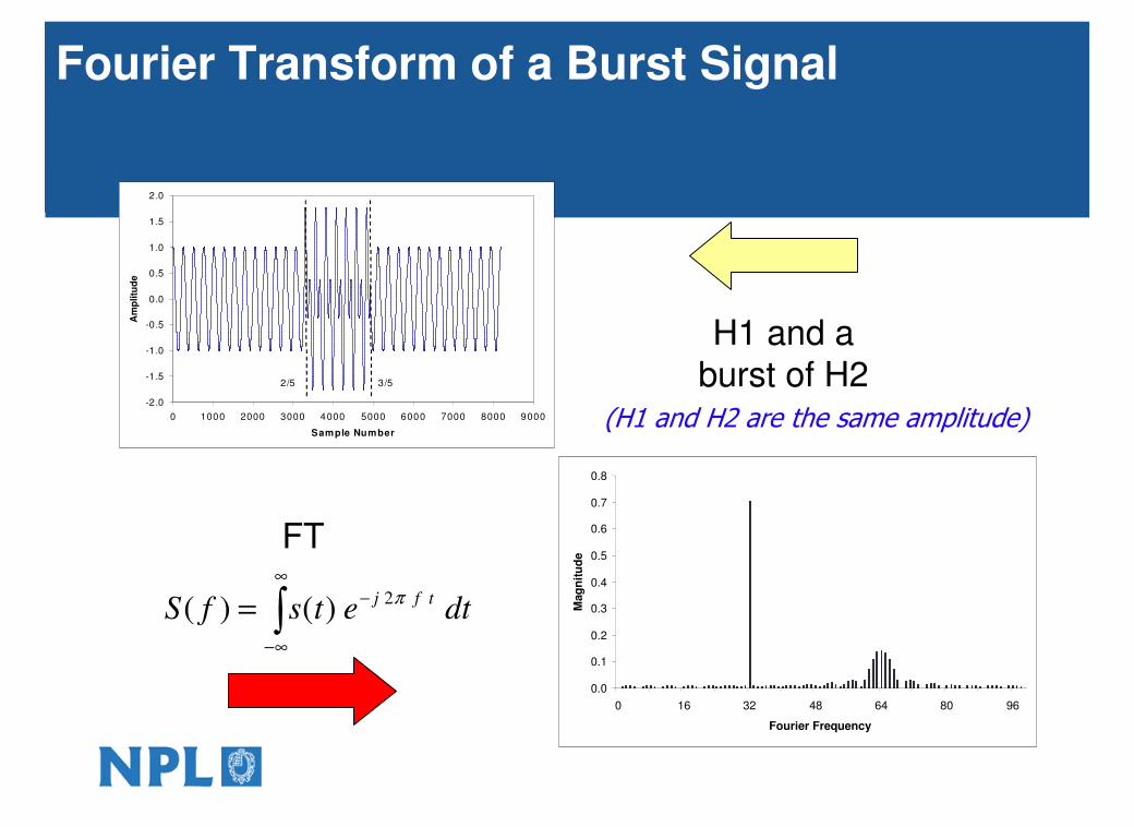
Fourier Transform of a Burst Signal

H1 and a

burst of H2

0.0

0.1

0.2

0.3

0.4

0.5

0.6

0.7

0.8

0 16 32 48 64 80 96

Fourier Frequency

Mag

nit

ud

e

-2.0

-1.5

-1.0

-0.5

0.0

0.5

1.0

1.5

2.0

0 1000 2000 3000 4000 5000 6000 7000 8000 9000

Sample Number

Am

plitu

de

2/5 3/5

(H1 and H2 are the same amplitude)

FT

∫−∞

∞−

−= dtetsfStfj π2)()(

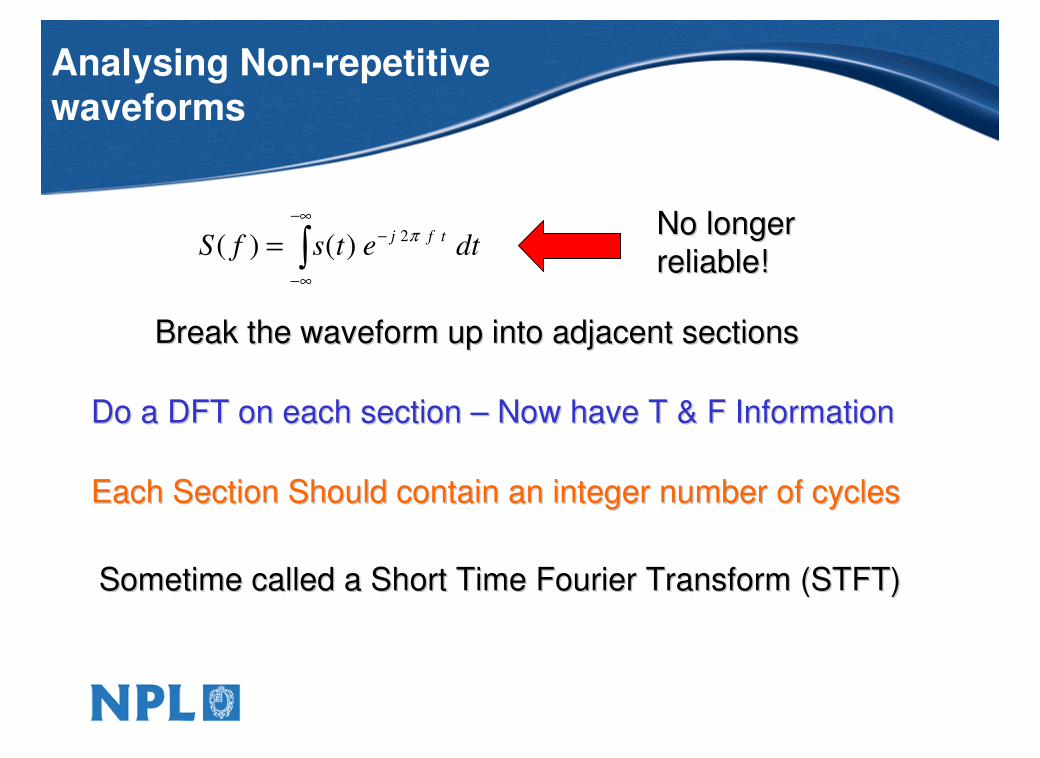
Analysing Non-repetitive

waveforms

Break the waveform up into adjacent sectionsBreak the waveform up into adjacent sections

Do a DFT on each section Do a DFT on each section –– Now have T & F InformationNow have T & F Information

Each Section Should contain an integer number of cyclesEach Section Should contain an integer number of cycles

Sometime called a Short Time Fourier Transform (STFT)Sometime called a Short Time Fourier Transform (STFT)

∫−∞

∞−

−= dtetsfStfj π2)()(

No longer No longer

reliable!reliable!

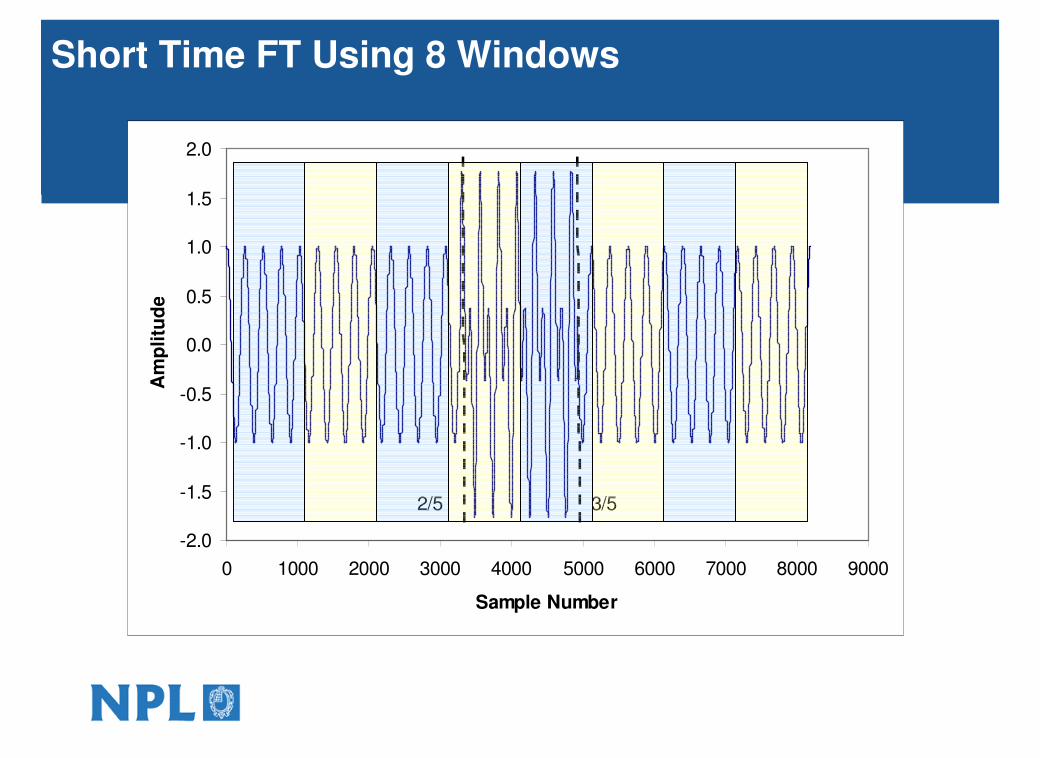
Short Time FT Using 8 Windows

-2.0

-1.5

-1.0

-0.5

0.0

0.5

1.0

1.5

2.0

0 1000 2000 3000 4000 5000 6000 7000 8000 9000

Sample Number

Am

plitu

de

2/5 3/5

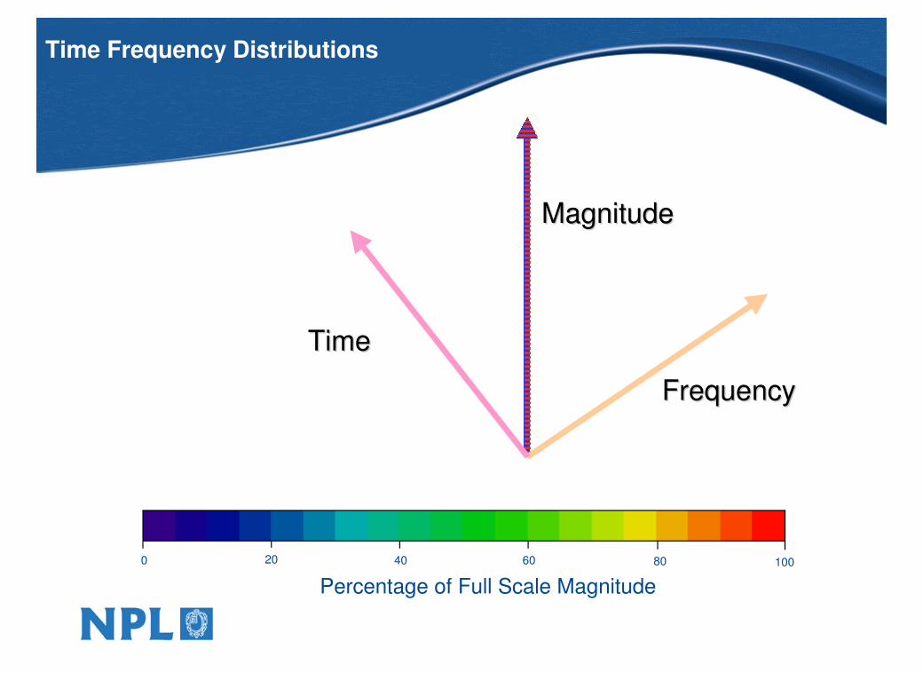
Time Frequency Distributions

TimeTime

FrequencyFrequency

MagnitudeMagnitude

Percentage of Full Scale Magnitude

0 40 60 80 10020

STFT Using 8 Windows

2/5

3/5

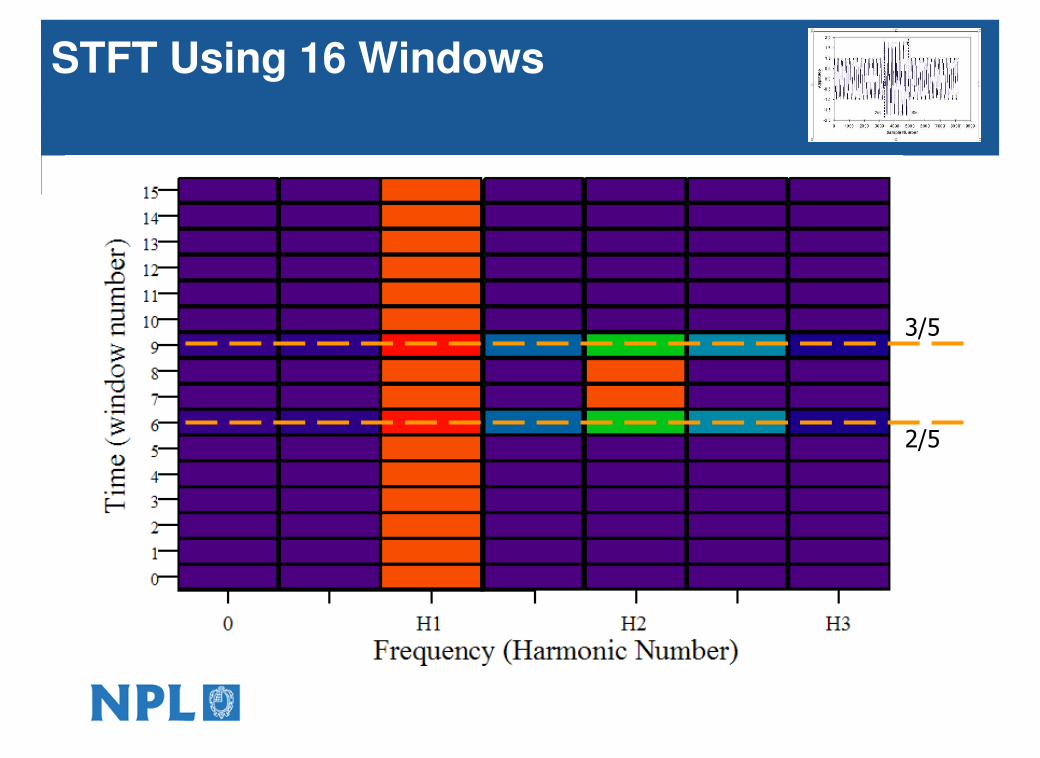
STFT Using 16 Windows

2/5

3/5

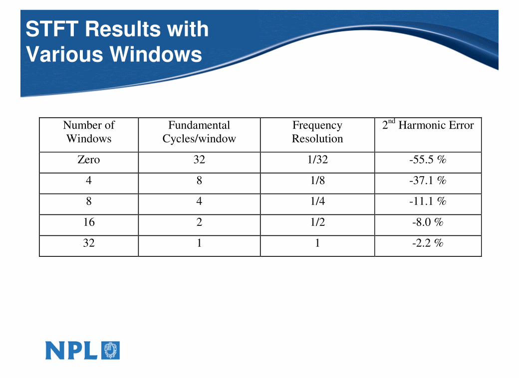
Number of

Windows

Fundamental

Cycles/window

Frequency

Resolution

2nd

Harmonic Error

Zero 32 1/32 -55.5 %

4 8 1/8 -37.1 %

8 4 1/4 -11.1 %

16 2 1/2 -8.0 %

32 1 1 -2.2 %

STFT Results with Various Windows

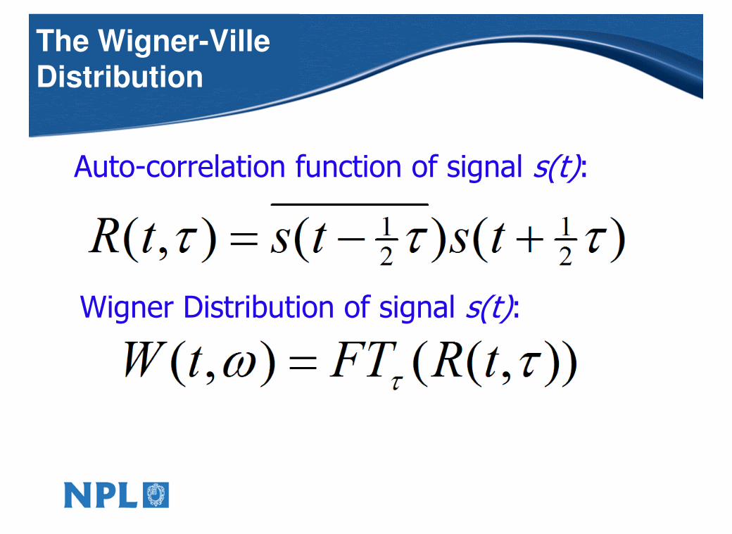
The Wigner-Ville Distribution

Auto-correlation function of signal s(t):

Wigner Distribution of signal s(t):

Analysis of a Burst

16 Window STFT

Wigner Ville Distribution

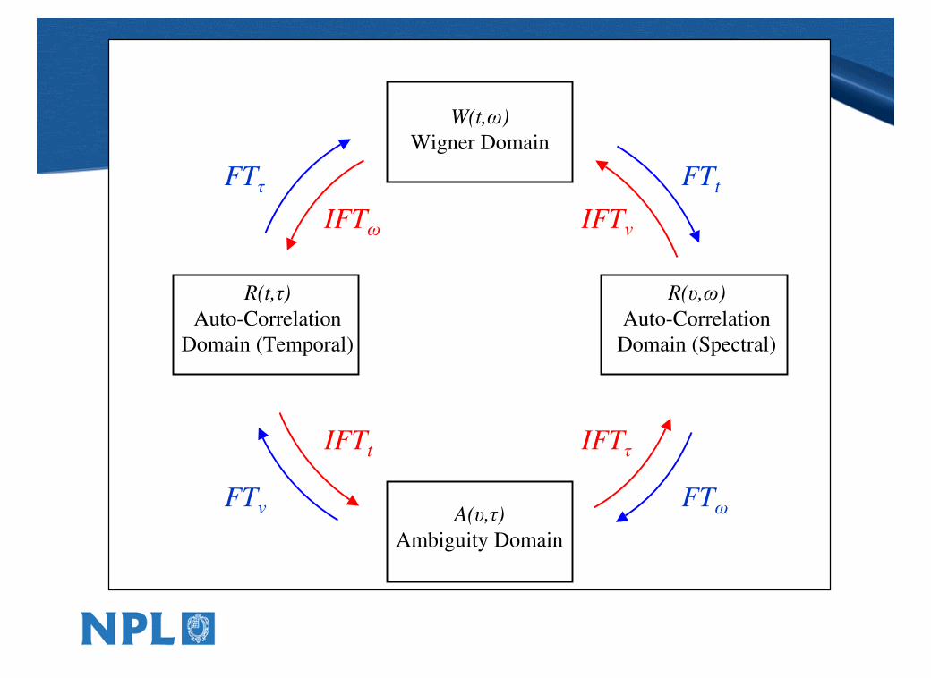
FTν

FTω

FTτ

FTt

IFTt

IFTω

IFTν

IFTτ

W(t,ω)

Wigner Domain

R(t,τ)

Auto-Correlation

Domain (Temporal)

R(υ,ω)

Auto-Correlation

Domain (Spectral)

A(υ,τ)

Ambiguity Domain

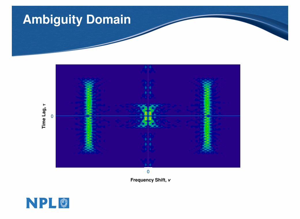
Frequency Shift, ν

Tim

e L

ag

, τ

0

0

Ambiguity Domain

Frequency Shift, ν

Time Lag, τ

Ma

gn

itud

e

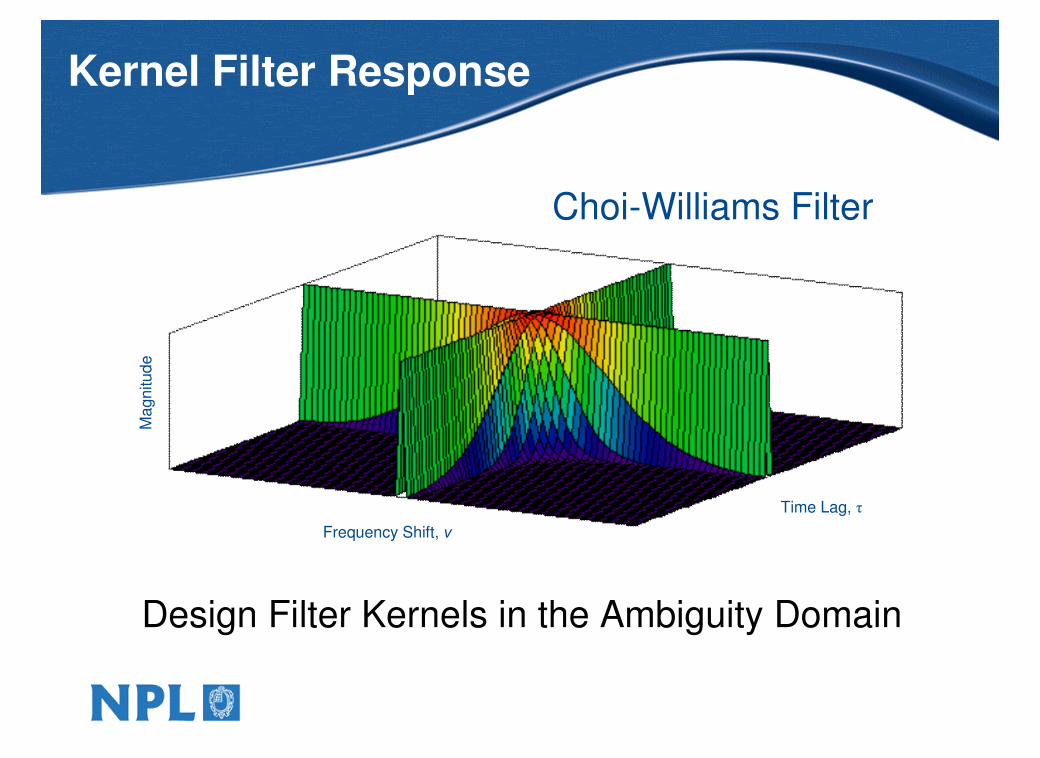
Kernel Filter Response

Design Filter Kernels in the Ambiguity Domain

Choi-Williams Filter

Tim

e L

ag

, τ

0

Frequency Shift, ν

0

Filtered Ambiguity

Function

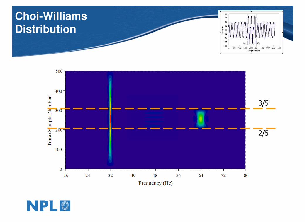
Choi-Williams

Distribution

2/5

3/5

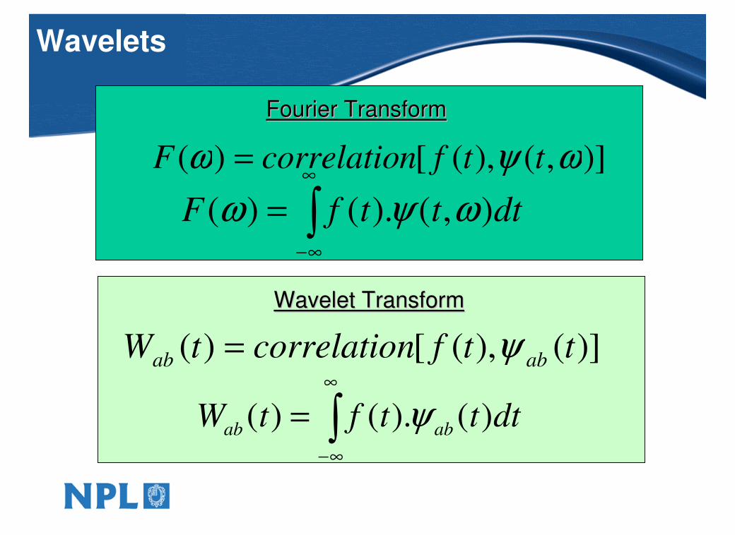
Wavelets

)],(),([)( ωψω ttfncorrelatioF =

∫∞

∞−

= dtttfF ),().()( ωψω

Fourier TransformFourier Transform

)](),([)( ttfncorrelatiotW abab ψ=

∫∞

∞−

= dtttftWabab

)().()( ψ

Wavelet TransformWavelet Transform

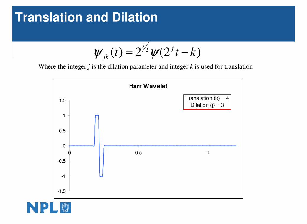
Translation and Dilation

)2(2)( 2 kttj

jk

j

−= ψψWhere the integer j is the dilation parameter and integer k is used for translation

Harr Wavelet

-1.5

-1

-0.5

0

0.5

1

1.5

0 0.5 1

Translation (k) = 1

Dilation (j) = 1

Harr Wavelet

-1.5

-1

-0.5

0

0.5

1

1.5

0 0.5 1

Translation (k) = 1

Dilation (j) = 2

Harr Wavelet

-1.5

-1

-0.5

0

0.5

1

1.5

0 0.5 1

Translation (k) = 2

Dilation (j) = 2

Harr Wavelet

-1.5

-1

-0.5

0

0.5

1

1.5

0 0.5 1

Translation (k) = 3

Dilation (j) = 2

Harr Wavelet

-1.5

-1

-0.5

0

0.5

1

1.5

0 0.5 1

Translation (k) = 3

Dilation (j) = 3

Harr Wavelet

-1.5

-1

-0.5

0

0.5

1

1.5

0 0.5 1

Translation (k) = 4

Dilation (j) = 3

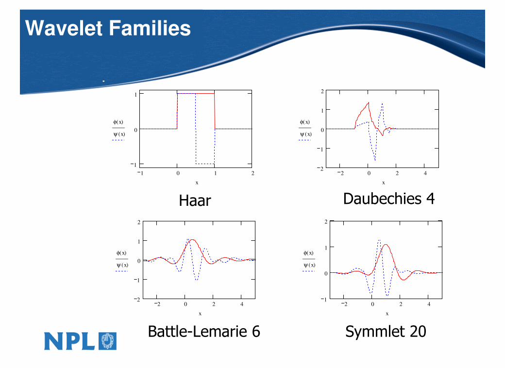
Wavelet Families

1 0 1 2

1

0

1

φ x( )

ψ x( )

x

Haar

2 0 2 42

1

0

1

2

φ x( )

ψ x( )

x

Daubechies 4

2 0 2 41

0

1

2

φ x( )

ψ x( )

x

Symmlet 20Battle-Lemarie 6

2 0 2 42

1

0

1

2

φ x( )

ψ x( )

x

Vibration Analysis Using Wavelets

D 1 1

D 1 0

D 9

D 8

D 7

D 6

D 5

D 4

D 3

S a m p le N u m b e r

Frequency

Amplitude (with arb. offsets)

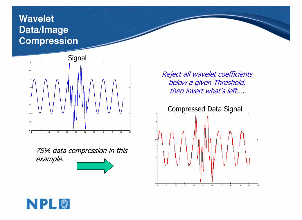
Wavelet Data/Image Compression

Reject all wavelet coefficients below a given Threshold, then invert what’s left….

Signal

75% data compression in thisexample.

Compressed Data Signal

Perform DWT, retain only

highest 10 % of coefficients

Reconstructed Image –

10:1 compressionPerform DWT, retain only

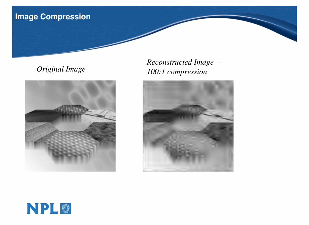
highest 1 % of coefficients

Reconstructed Image –

100:1 compression

Image Compression

Original Image

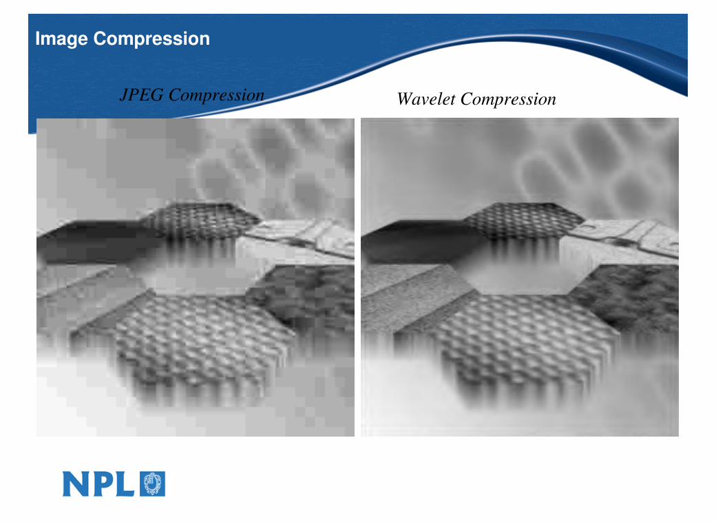
JPEG Compression Wavelet Compression

Image Compression

Fine Spatial Texture Image

Coarse Spatial Spectral Image

Fused Image

Wavelet Data/Image Fusion

(NB this is illustrative!)

Smooth Modulation

Made of H1, H2 and H3

But…

A Harmonic Modulation Model

∑∑==

+++=N

n

n

N

n

ntnqqtnpptx

1

0

1

0)(sin)(cos)( ωω

A signal x(t) with N non-modulated harmonics:

For modulated harmonics, use modulation functions

m(t) for the p’s & q’s:

pn(t) = an,0 m<0> + an,1 m

<1> + … an,K m<K>

qn(t) = bn,0 m<0> + bn,1 m

<1> + … bn,K m<K>

(if m<k> = tk then the scheme is a polynomial modulation model)

DeDe--modulate using Method of Least Squaresmodulate using Method of Least Squares

When m(t) = t, the modulators are polynomials,

Highly accurate demodulation for smooth modulation functions.

Polynomial modulation functionsPolynomial modulation functions

Using Wavelet Basis Functions

For signals with discontinuities, the m(t) functions can be wavelets…

-1.2

-0.8

-0.4

0

0.4

0.8

1.2

0 100 200 300 400 500

Sample Number

Am

plitu

de

Test Signal: Modulated H1 and H2

H1

H2

L.S. D4 Wavelet demodulation

High Accuracy Demodulation – Handles the discontinuity!

Summary

• Short Time Fourier Transforms

• Time Resolution – Frequency Resolution Trade Off

• Wigner Distributions

• Ambiguity Domain Filtering

• Wavelets

• Time Series Modulation Methods