An Introduction to Stata for Health

Researchers

Fourth Edition

SVEND JUUL

Department of Public Health

Section for Epidemiology

Aarhus University

Aarhus, Denmark

MORTEN FRYDENBERG

Department of Public Health

Section for Biostatistics

Aarhus University

Aarhus, Denmark

®

A Stata Press Publication

StataCorp LP

College Station, Texas

® Copyright c© 2006, 2008, 2010, 2014 by StataCorp LP

All rights reserved. First edition 2006

Second edition 2008

Third edition 2010

Fourth edition 2014

Published by Stata Press, 4905 Lakeway Drive, College Station, Texas 77845

Typeset in LATEX 2εPrinted in the United States of America

10 9 8 7 6 5 4 3 2 1

ISBN-10: 1-59718-135-8

ISBN-13: 978-1-59718-135-8

Library of Congress Control Number: 2014933534

No part of this book may be reproduced, stored in a retrieval system, or transcribed, in any form or

by any means—electronic, mechanical, photocopy, recording, or otherwise—without the prior written

permission of StataCorp LP.

Stata, , Stata Press, Mata, , and NetCourse are registered trademarks of

StataCorp LP.

Stata and Stata Press are registered trademarks with the World Intellectual Property Organization of the

United Nations.

LATEX 2ε is a trademark of the American Mathematical Society.

Contents

List of tables xi

List of figures xiii

Preface to the fourth edition xvii

Preface to the first edition xix

Online supplements xxi

Notations in this book xxiii

I The basics 1

1 Getting started 3

1.1 Installing and updating Stata . . . . . . . . . . . . . . . . . . . . . . . . 3

1.2 Starting and exiting Stata . . . . . . . . . . . . . . . . . . . . . . . . . . 7

1.3 Windows in Stata . . . . . . . . . . . . . . . . . . . . . . . . . . . . . . 8

1.4 Issuing commands . . . . . . . . . . . . . . . . . . . . . . . . . . . . . 14

1.5 Managing output . . . . . . . . . . . . . . . . . . . . . . . . . . . . . . 15

2 Getting help—and more 19

2.1 The help and search commands . . . . . . . . . . . . . . . . . . . . . . . 19

2.2 The PDF documentation . . . . . . . . . . . . . . . . . . . . . . . . . . 23

2.3 Other resources . . . . . . . . . . . . . . . . . . . . . . . . . . . . . . . 23

3 Stata file types and names 25

4 Command syntax 27

4.1 General syntax rules . . . . . . . . . . . . . . . . . . . . . . . . . . . . 27

4.2 Syntax diagrams . . . . . . . . . . . . . . . . . . . . . . . . . . . . . . . 27

4.3 Lists of variables and numbers . . . . . . . . . . . . . . . . . . . . . . . 29

4.4 Qualifiers . . . . . . . . . . . . . . . . . . . . . . . . . . . . . . . . . . 30

4.5 Weights . . . . . . . . . . . . . . . . . . . . . . . . . . . . . . . . . . . 32

vi Contents

4.6 Options . . . . . . . . . . . . . . . . . . . . . . . . . . . . . . . . . . . 32

4.7 Prefixes . . . . . . . . . . . . . . . . . . . . . . . . . . . . . . . . . . . 33

4.8 Other syntax elements . . . . . . . . . . . . . . . . . . . . . . . . . . . . 34

4.9 Version control . . . . . . . . . . . . . . . . . . . . . . . . . . . . . . . 35

4.10 Errors and error messages . . . . . . . . . . . . . . . . . . . . . . . . . . 36

II Data management 39

5 Variables 41

5.1 Numeric formats . . . . . . . . . . . . . . . . . . . . . . . . . . . . . . 41

5.2 Missing values . . . . . . . . . . . . . . . . . . . . . . . . . . . . . . . 42

5.3 Storage types and precision . . . . . . . . . . . . . . . . . . . . . . . . . 44

5.4 Date and time variables . . . . . . . . . . . . . . . . . . . . . . . . . . . 47

5.5 String variables . . . . . . . . . . . . . . . . . . . . . . . . . . . . . . . 50

5.6 Memory considerations . . . . . . . . . . . . . . . . . . . . . . . . . . . 54

6 Getting data in and out of Stata 55

6.1 Opening and saving Stata data . . . . . . . . . . . . . . . . . . . . . . . 55

6.2 Entering data . . . . . . . . . . . . . . . . . . . . . . . . . . . . . . . . 59

6.3 Exchanging data with other software . . . . . . . . . . . . . . . . . . . . 60

7 Documentation commands 65

7.1 Labels . . . . . . . . . . . . . . . . . . . . . . . . . . . . . . . . . . . . 65

8 Calculations 69

8.1 generate and replace . . . . . . . . . . . . . . . . . . . . . . . . . . . . 69

8.2 Operators and functions in calculations . . . . . . . . . . . . . . . . . . . 71

8.3 The egen command . . . . . . . . . . . . . . . . . . . . . . . . . . . . . 73

8.4 Recoding variables . . . . . . . . . . . . . . . . . . . . . . . . . . . . . 75

8.5 Checking correctness of calculations . . . . . . . . . . . . . . . . . . . . 76

8.6 Giving numbers to observations . . . . . . . . . . . . . . . . . . . . . . 77

9 Commands affecting data structure 81

9.1 Selecting observations and variables . . . . . . . . . . . . . . . . . . . . 81

9.2 Renaming and reordering variables . . . . . . . . . . . . . . . . . . . . . 82

Contents vii

9.3 Sorting data . . . . . . . . . . . . . . . . . . . . . . . . . . . . . . . . . 82

9.4 Combining files . . . . . . . . . . . . . . . . . . . . . . . . . . . . . . . 83

9.5 Reshaping data . . . . . . . . . . . . . . . . . . . . . . . . . . . . . . . 87

10 Taking good care of your data 93

10.1 The audit trail . . . . . . . . . . . . . . . . . . . . . . . . . . . . . . . . 93

10.2 Collecting and entering data . . . . . . . . . . . . . . . . . . . . . . . . 94

10.3 Data management . . . . . . . . . . . . . . . . . . . . . . . . . . . . . . 99

10.4 Analysis . . . . . . . . . . . . . . . . . . . . . . . . . . . . . . . . . . . 106

10.5 Protect your data . . . . . . . . . . . . . . . . . . . . . . . . . . . . . . 108

10.6 Archiving the project . . . . . . . . . . . . . . . . . . . . . . . . . . . . 110

III Analysis 113

11 Description and simple analysis 115

11.1 Overview of a dataset . . . . . . . . . . . . . . . . . . . . . . . . . . . . 115

11.2 Listing observations . . . . . . . . . . . . . . . . . . . . . . . . . . . . . 118

11.3 Simple tables for categorical variables . . . . . . . . . . . . . . . . . . . 120

11.4 Epidemiologic tables . . . . . . . . . . . . . . . . . . . . . . . . . . . . 125

11.5 Analyzing continuous variables . . . . . . . . . . . . . . . . . . . . . . . 133

11.6 Finding confidence intervals . . . . . . . . . . . . . . . . . . . . . . . . 141

11.7 Immediate commands . . . . . . . . . . . . . . . . . . . . . . . . . . . . 142

12 Regression analysis 145

12.1 Linear regression . . . . . . . . . . . . . . . . . . . . . . . . . . . . . . 145

12.2 Regression postestimation . . . . . . . . . . . . . . . . . . . . . . . . . 148

12.3 Categorical predictors—factor variables . . . . . . . . . . . . . . . . . . 150

12.4 Interactions in regression models . . . . . . . . . . . . . . . . . . . . . . 155

12.5 Logistic regression . . . . . . . . . . . . . . . . . . . . . . . . . . . . . 162

12.6 Other regression models . . . . . . . . . . . . . . . . . . . . . . . . . . 167

12.7 Nonindependent observations . . . . . . . . . . . . . . . . . . . . . . . . 168

13 Time-to-event data 171

13.1 Setting the time scale and event: The stset command . . . . . . . . . . . 173

viii Contents

13.2 The Kaplan–Meier survival function . . . . . . . . . . . . . . . . . . . . 175

13.3 Tabulating rates . . . . . . . . . . . . . . . . . . . . . . . . . . . . . . . 178

13.4 Cox proportional hazards regression . . . . . . . . . . . . . . . . . . . . 181

13.5 Preparing data for advanced survival analyses . . . . . . . . . . . . . . . 186

13.6 Advanced survival modeling . . . . . . . . . . . . . . . . . . . . . . . . 189

13.7 Poisson regression . . . . . . . . . . . . . . . . . . . . . . . . . . . . . 192

13.8 Standardization . . . . . . . . . . . . . . . . . . . . . . . . . . . . . . . 195

14 Measurement and diagnosis 199

14.1 Comparing two measurements . . . . . . . . . . . . . . . . . . . . . . . 199

14.2 Reproducibility of measurements . . . . . . . . . . . . . . . . . . . . . . 203

14.3 Using tests for diagnosis . . . . . . . . . . . . . . . . . . . . . . . . . . 206

15 Miscellaneous 213

15.1 Random samples, simulations . . . . . . . . . . . . . . . . . . . . . . . 213

15.2 Power and sample-size analysis . . . . . . . . . . . . . . . . . . . . . . . 215

15.3 Commands that influence program flow . . . . . . . . . . . . . . . . . . 220

15.4 Decimal periods and commas . . . . . . . . . . . . . . . . . . . . . . . . 221

15.5 Logging output permanently . . . . . . . . . . . . . . . . . . . . . . . . 223

15.6 Other analyses . . . . . . . . . . . . . . . . . . . . . . . . . . . . . . . . 225

IV Graphs 227

16 Graphs 229

16.1 Anatomy of a graph . . . . . . . . . . . . . . . . . . . . . . . . . . . . . 230

16.2 Anatomy of graph commands . . . . . . . . . . . . . . . . . . . . . . . . 231

16.3 Graph size . . . . . . . . . . . . . . . . . . . . . . . . . . . . . . . . . . 232

16.4 Schemes . . . . . . . . . . . . . . . . . . . . . . . . . . . . . . . . . . . 235

16.5 Graph options: Axes . . . . . . . . . . . . . . . . . . . . . . . . . . . . 237

16.6 Graph options: Text elements . . . . . . . . . . . . . . . . . . . . . . . . 242

16.7 Plot options: Markers, lines, etc. . . . . . . . . . . . . . . . . . . . . . . 246

16.8 Histograms and other distribution graphs . . . . . . . . . . . . . . . . . . 249

16.9 Twoway plots: scatterplots and line plots . . . . . . . . . . . . . . . . . . 253

Contents ix

16.10 Bar graphs . . . . . . . . . . . . . . . . . . . . . . . . . . . . . . . . . . 264

16.11 By-graphs and combined graphs . . . . . . . . . . . . . . . . . . . . . . 269

16.12 Saving and exporting graphs . . . . . . . . . . . . . . . . . . . . . . . . 272

V Advanced topics 275

17 Advanced topics 277

17.1 Using stored results . . . . . . . . . . . . . . . . . . . . . . . . . . . . . 277

17.2 Macros and scalars . . . . . . . . . . . . . . . . . . . . . . . . . . . . . 282

17.3 Some useful commands . . . . . . . . . . . . . . . . . . . . . . . . . . . 284

17.4 Programs . . . . . . . . . . . . . . . . . . . . . . . . . . . . . . . . . . 288

17.5 Debugging programs . . . . . . . . . . . . . . . . . . . . . . . . . . . . 292

VI Appendixes 293

A Stata manuals 295

B Exercises 297

B.1 The user interface . . . . . . . . . . . . . . . . . . . . . . . . . . . . . . 298

B.2 Managing output . . . . . . . . . . . . . . . . . . . . . . . . . . . . . . 300

B.3 Calculations . . . . . . . . . . . . . . . . . . . . . . . . . . . . . . . . . 301

B.4 Working with missing values . . . . . . . . . . . . . . . . . . . . . . . . 304

B.5 Working with date variables . . . . . . . . . . . . . . . . . . . . . . . . 304

B.6 Description and simple analysis . . . . . . . . . . . . . . . . . . . . . . 305

B.7 Taking good care of your data . . . . . . . . . . . . . . . . . . . . . . . 306

C Shortcuts and keystrokes 309

References 311

Author index 313

Subject index 315

Preface to the fourth edition

This fourth edition updates the third edition to reflect the changes in Stata 12, released in July

2011, and Stata 13, released in June 2013.

Since the first edition of the book, many nice things have happened with Stata, and these changes

are also reflected in the book. One of the nice developments is the PDF manuals, which give

you immediate access to “everything” about Stata. While previous editions of the book included

lots of references to specific entries in the manuals, you find few such references in the present

edition. Instead, you are guided to use the help command, which efficiently leads you to the

information you need. This also means that the text reads much more fluently.

In several other ways, Stata has become more user friendly, which means that we could drop

quite a bit of tedious stuff from the book. We need no longer explain the set memory command

or the importance of the update swap command. And we need no longer explain that when

the Data Editor is open, you cannot do anything else in Stata.

Among other important developments are the introduction of factor variables (Stata 11), date-

and-time variables (Stata 10), and a much improved merge command (Stata 11).

This is an introductory book aimed at people working in health research, and we have made

several decisions about what to include and what to omit. If you miss something that is not

described in the book, it does not necessarily mean that Stata cannot do it. In appendix A, you

will find an overview of the Stata documentation illustrating the breadth of Stata.

The former versions of the book were written for Windows users only. In this edition, we have

included information for Mac users.

David Culwell at StataCorp took care of the technical editing, Bill Rising gave several useful

suggestions to improve the quality of the book, and Lisa Gilmore coordinated everything.

User reactions are welcome and can be good inspiration for further improvements, so please

feel free to send comments to sj@soci.au.dk or morten@biostat.au.dk.

Aarhus, Denmark Svend Juul and Morten Frydenberg

February 2014

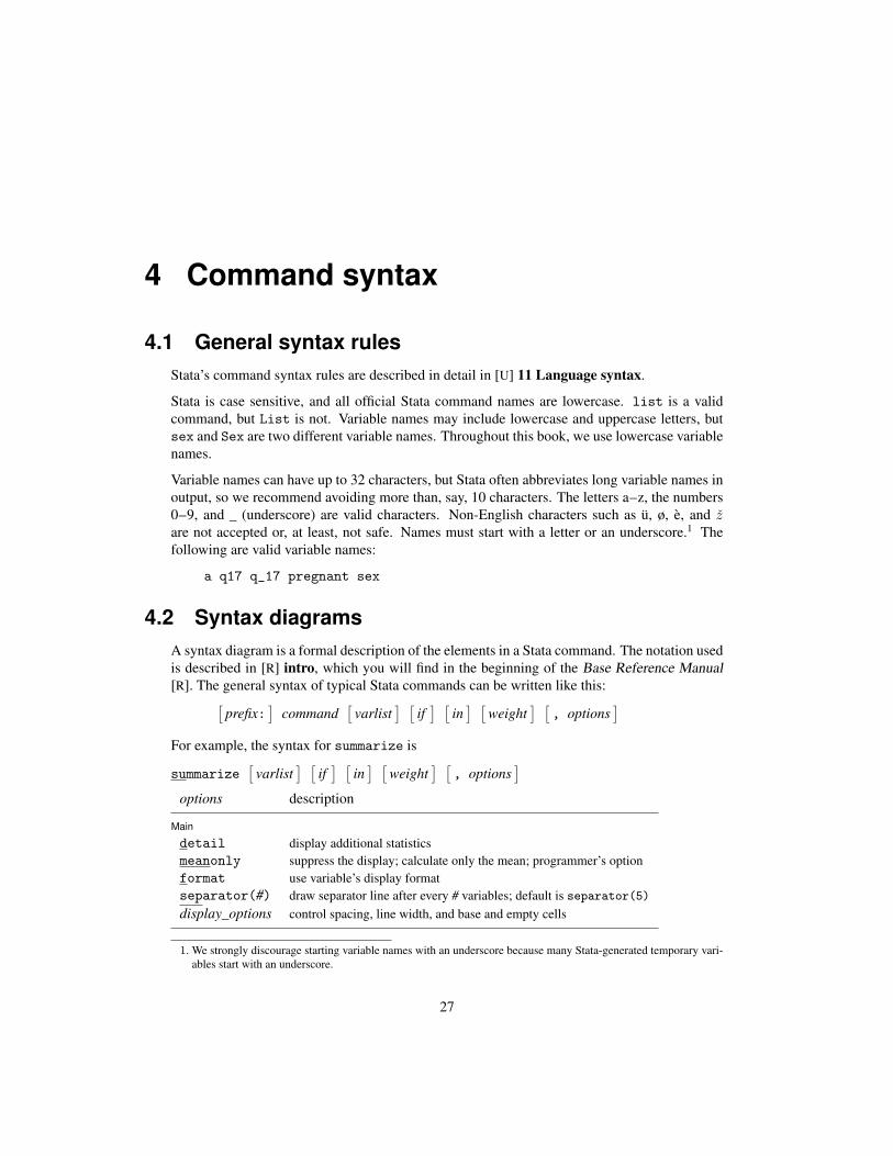
4 Command syntax

4.1 General syntax rules

Stata’s command syntax rules are described in detail in [U] 11 Language syntax.

Stata is case sensitive, and all official Stata command names are lowercase. list is a valid

command, but List is not. Variable names may include lowercase and uppercase letters, but

sex and Sex are two different variable names. Throughout this book, we use lowercase variable

names.

Variable names can have up to 32 characters, but Stata often abbreviates long variable names in

output, so we recommend avoiding more than, say, 10 characters. The letters a–z, the numbers

0–9, and _ (underscore) are valid characters. Non-English characters such as ü, ø, è, and zare not accepted or, at least, not safe. Names must start with a letter or an underscore.1 The

following are valid variable names:

a q17 q_17 pregnant sex

4.2 Syntax diagrams

A syntax diagram is a formal description of the elements in a Stata command. The notation used

is described in [R] intro, which you will find in the beginning of the Base Reference Manual

[R]. The general syntax of typical Stata commands can be written like this:[

prefix:]

command[

varlist] [

if] [

in] [

weight] [

, options]

For example, the syntax for summarize is

summarize[

varlist] [

if] [

in] [

weight] [

, options]

options description

Main

detail display additional statistics

meanonly suppress the display; calculate only the mean; programmer’s option

format use variable’s display format

separator(#) draw separator line after every # variables; default is separator(5)

display_options control spacing, line width, and base and empty cells

1. We strongly discourage starting variable names with an underscore because many Stata-generated temporary vari-

ables start with an underscore.

27

28 Chapter 4 Command syntax

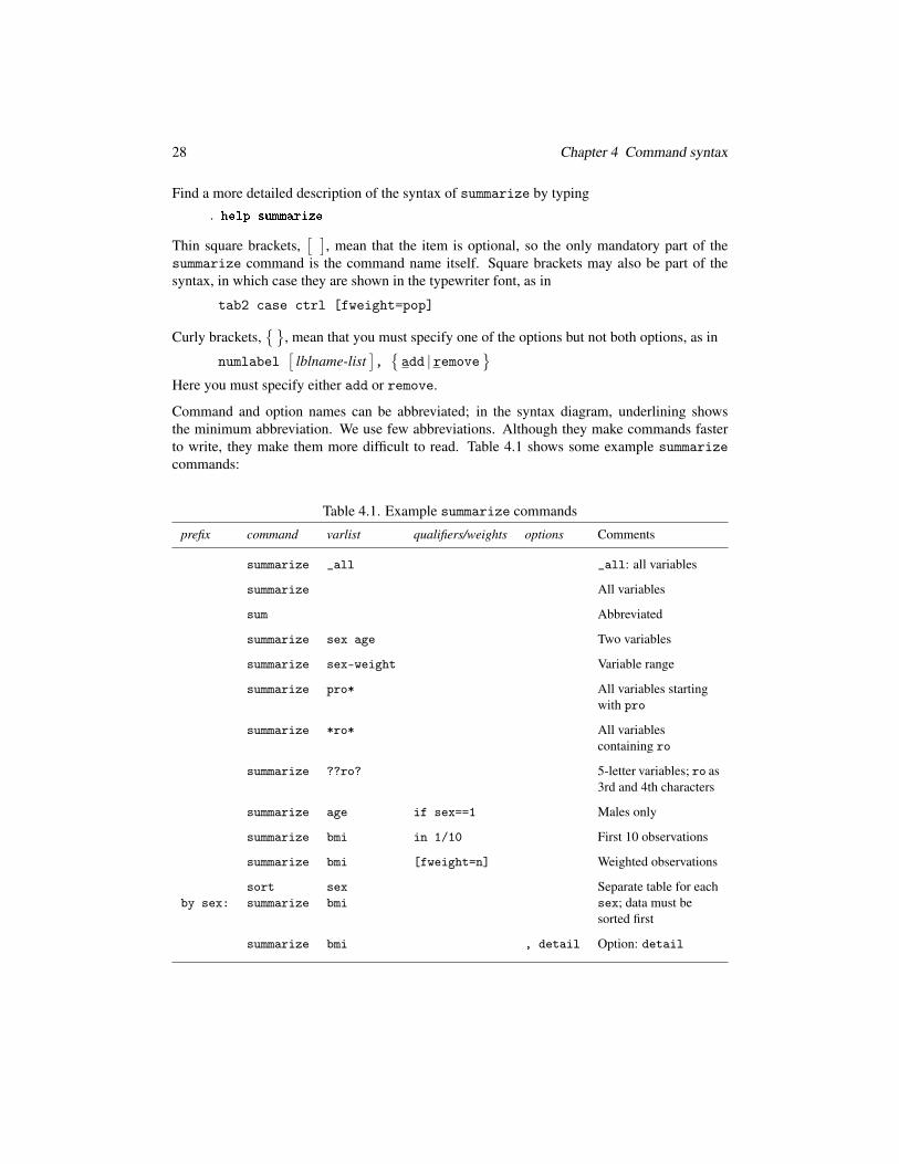
Find a more detailed description of the syntax of summarize by typing

. help summarizeThin square brackets,

[ ]

, mean that the item is optional, so the only mandatory part of the

summarize command is the command name itself. Square brackets may also be part of the

syntax, in which case they are shown in the typewriter font, as in

tab2 case ctrl [fweight=pop]

Curly brackets,{}

, mean that you must specify one of the options but not both options, as in

numlabel[

lblname-list]

,{

add | remove}

Here you must specify either add or remove.

Command and option names can be abbreviated; in the syntax diagram, underlining shows

the minimum abbreviation. We use few abbreviations. Although they make commands faster

to write, they make them more difficult to read. Table 4.1 shows some example summarize

commands:

Table 4.1. Example summarize commands

prefix command varlist qualifiers/weights options Comments

summarize _all _all: all variables

summarize All variables

sum Abbreviated

summarize sex age Two variables

summarize sex-weight Variable range

summarize pro* All variables starting

with pro

summarize *ro* All variables

containing ro

summarize ??ro? 5-letter variables; ro as

3rd and 4th characters

summarize age if sex==1 Males only

summarize bmi in 1/10 First 10 observations

summarize bmi [fweight=n] Weighted observations

sort sex Separate table for each

by sex: summarize bmi sex; data must be

sorted first

summarize bmi , detail Option: detail

4.3 Lists of variables and numbers 29

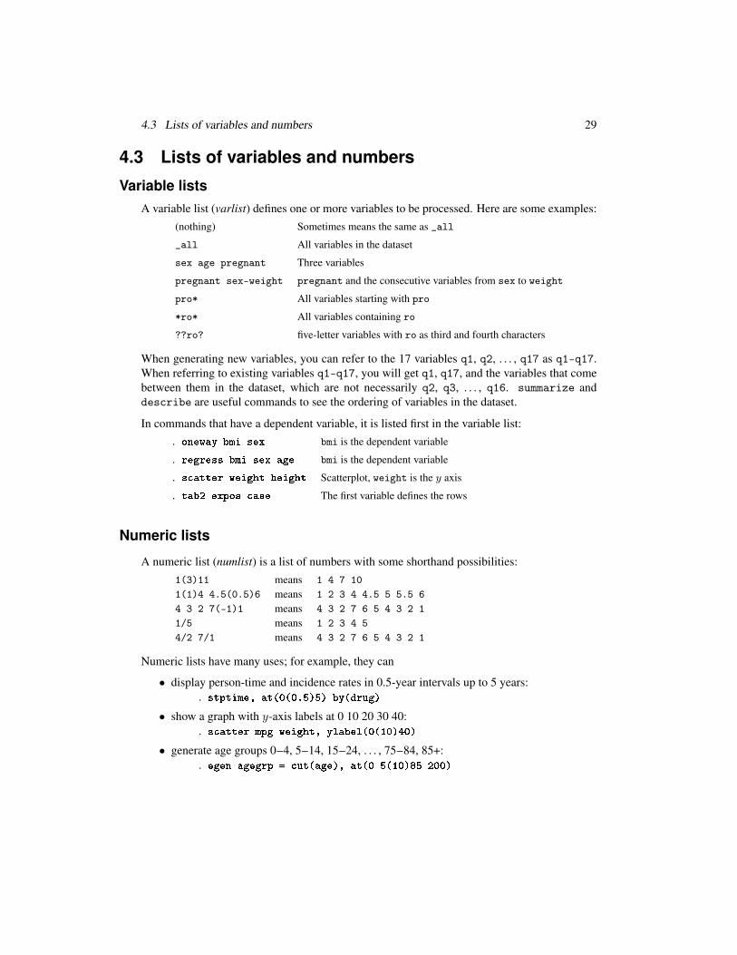
4.3 Lists of variables and numbers

Variable lists

A variable list (varlist) defines one or more variables to be processed. Here are some examples:

(nothing) Sometimes means the same as _all

_all All variables in the dataset

sex age pregnant Three variables

pregnant sex-weight pregnant and the consecutive variables from sex to weight

pro* All variables starting with pro

*ro* All variables containing ro

??ro? five-letter variables with ro as third and fourth characters

When generating new variables, you can refer to the 17 variables q1, q2, . . . , q17 as q1-q17.

When referring to existing variables q1-q17, you will get q1, q17, and the variables that come

between them in the dataset, which are not necessarily q2, q3, . . . , q16. summarize and

describe are useful commands to see the ordering of variables in the dataset.

In commands that have a dependent variable, it is listed first in the variable list:

. oneway bmi sex bmi is the dependent variable

. regress bmi sex age bmi is the dependent variable

. s atter weight height Scatterplot, weight is the y axis

. tab2 expos ase The first variable defines the rows

Numeric lists

A numeric list (numlist) is a list of numbers with some shorthand possibilities:

1(3)11 means 1 4 7 10

1(1)4 4.5(0.5)6 means 1 2 3 4 4.5 5 5.5 6

4 3 2 7(-1)1 means 4 3 2 7 6 5 4 3 2 1

1/5 means 1 2 3 4 5

4/2 7/1 means 4 3 2 7 6 5 4 3 2 1

Numeric lists have many uses; for example, they can

• display person-time and incidence rates in 0.5-year intervals up to 5 years:

. stptime, at(0(0.5)5) by(drug)• show a graph with y-axis labels at 0 10 20 30 40:

. s atter mpg weight, ylabel(0(10)40)• generate age groups 0–4, 5–14, 15–24, . . . , 75–84, 85+:

. egen agegrp = ut(age), at(0 5(10)85 200)

30 Chapter 4 Command syntax

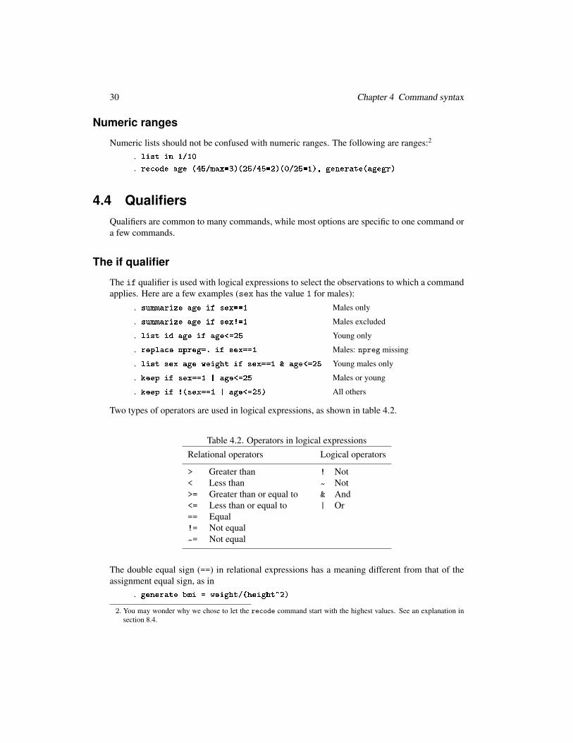
Numeric ranges

Numeric lists should not be confused with numeric ranges. The following are ranges:2

. list in 1/10

. re ode age (45/max=3)(25/45=2)(0/25=1), generate(agegr)4.4 Qualifiers

Qualifiers are common to many commands, while most options are specific to one command or

a few commands.

The if qualifier

The if qualifier is used with logical expressions to select the observations to which a command

applies. Here are a few examples (sex has the value 1 for males):

. summarize age if sex==1 Males only

. summarize age if sex!=1 Males excluded

. list id age if age<=25 Young only

. repla e npreg=. if sex==1 Males: npreg missing

. list sex age weight if sex==1 & age<=25 Young males only

. keep if sex==1 | age<=25 Males or young

. keep if !(sex==1 | age<=25) All others

Two types of operators are used in logical expressions, as shown in table 4.2.

Table 4.2. Operators in logical expressions

Relational operators Logical operators

> Greater than ! Not

< Less than ~ Not

>= Greater than or equal to & And

<= Less than or equal to | Or

== Equal

!= Not equal

~= Not equal

The double equal sign (==) in relational expressions has a meaning different from that of the

assignment equal sign, as in

. generate bmi = weight/(height^2)2. You may wonder why we chose to let the recode command start with the highest values. See an explanation in

section 8.4.

4.4 Qualifiers 31

Logical expressions are evaluated to be true or false. A value of 0 means false, and any other

value, including missing values, means true. Technically, missing values are large positive

numbers and are evaluated as such in logical expressions. This issue is described in more detail

in section 5.2.

With complex logical expressions, use parentheses to control the order of evaluation:3

. anycommand if ((sex==1 & weight>90) | (sex==2 & weight>80))> & ! missing(weight)Omitting the parentheses might give a different selection, but the outcome may be difficult to

predict. Use parentheses to make the syntax transparent to yourself; then it will work correctly.

A possibly more transparent way to handle complex selections is to generate a help variable

(heavy):

. generate heavy=0 Initialize help variable

. repla e heavy=1 if sex==1 & weight>90 Include males > 90 kg

. repla e heavy=1 if sex==2 & weight>80 Include females > 80 kg

. repla e heavy=. if missing(weight) Do not include if weight is missing

. anycommand if heavy==1 These are the heavy ones

The in qualifier

The in qualifier is used to select the observations to which a command applies. It is especially

useful for listing or displaying a subset of observations. Below are three examples:

. list sex age weight in 23 23rd observation

. list in 1/10 All variables; observations 1–10

. browse sex-weight in -5/-1 See last 5 observations in the Data Browser

The last observation is identified by -1, and -5/-1 means the last five observations. Note that

the sort order of the dataset may change, so you should not rely on the observation number to

identify a specific observation.

3. In output, long command lines are wrapped. The initial character, ">", in the second line tells that this is a contin-

uation; ">" is not part of the command.

32 Chapter 4 Command syntax

4.5 Weights

Weighting observations

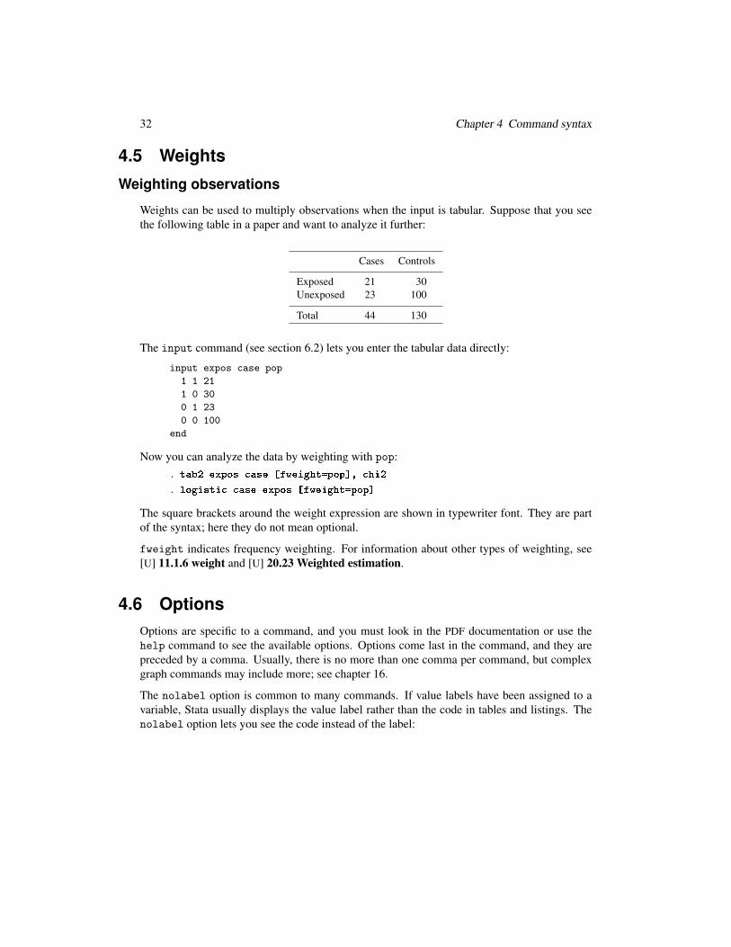
Weights can be used to multiply observations when the input is tabular. Suppose that you see

the following table in a paper and want to analyze it further:

Cases Controls

Exposed 21 30

Unexposed 23 100

Total 44 130

The input command (see section 6.2) lets you enter the tabular data directly:

input expos case pop

1 1 21

1 0 30

0 1 23

0 0 100

end

Now you can analyze the data by weighting with pop:

. tab2 expos ase [fweight=pop℄, hi2

. logisti ase expos [fweight=pop℄The square brackets around the weight expression are shown in typewriter font. They are part

of the syntax; here they do not mean optional.

fweight indicates frequency weighting. For information about other types of weighting, see

[U] 11.1.6 weight and [U] 20.23 Weighted estimation.

4.6 Options

Options are specific to a command, and you must look in the PDF documentation or use the

help command to see the available options. Options come last in the command, and they are

preceded by a comma. Usually, there is no more than one comma per command, but complex

graph commands may include more; see chapter 16.

The nolabel option is common to many commands. If value labels have been assigned to a

variable, Stata usually displays the value label rather than the code in tables and listings. The

nolabel option lets you see the code instead of the label:

4.7 Prefixes 33

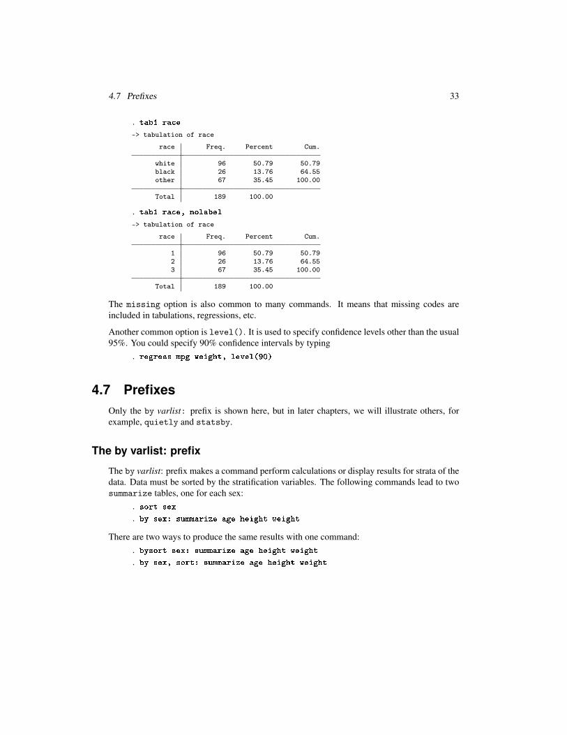
. tab1 ra e-> tabulation of race

race Freq. Percent Cum.

white 96 50.79 50.79black 26 13.76 64.55other 67 35.45 100.00

Total 189 100.00

. tab1 ra e, nolabel-> tabulation of race

race Freq. Percent Cum.

1 96 50.79 50.792 26 13.76 64.553 67 35.45 100.00

Total 189 100.00

The missing option is also common to many commands. It means that missing codes are

included in tabulations, regressions, etc.

Another common option is level(). It is used to specify confidence levels other than the usual

95%. You could specify 90% confidence intervals by typing

. regress mpg weight, level(90)4.7 Prefixes

Only the by varlist: prefix is shown here, but in later chapters, we will illustrate others, for

example, quietly and statsby.

The by varlist: prefix

The by varlist: prefix makes a command perform calculations or display results for strata of the

data. Data must be sorted by the stratification variables. The following commands lead to two

summarize tables, one for each sex:

. sort sex

. by sex: summarize age height weightThere are two ways to produce the same results with one command:

. bysort sex: summarize age height weight

. by sex, sort: summarize age height weight

12 Regression analysis

This chapter describes the fundamentals of linear regression and logistic regression. However,

many other regression models are available in Stata. Chapter 13 discusses Poisson regression

and Cox regression, and the general principles apply to them, too.

We will not go into details of how to analyze data by regression models, but instead, we will

focus on some of the features in Stata: working with categorical explanatory variables, testing

hypotheses and using Stata’s postestimation facilities.

Automatic selection procedures are available in Stata, but they will, in general, lead to invalid

estimates, confidence intervals, and p-values. Therefore, we will not describe them. Find a

discussion of the problems at http://www.stata.com/support/faqs/statistics/stepwise-regression-

problems/, What are some of the problems with stepwise regression?

A regression model expresses the dependency of one variable (the response, outcome, or depen-

dent variable) on one or more other variables (predictors, regressors, or independent variables).

Short introductions to regression models can be found in many standard textbooks, such as

Kirkwood and Sterne (2003). If you want to apply more than the simplest regression mod-

els, you should consult books dedicated to the subject, such as Vittinghoff et al. (2012) and

Hosmer et al. (2013). .

12.1 Linear regression

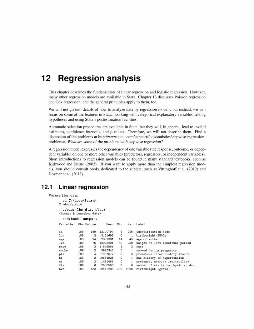
We use lbw.dta:

. d C:\do s\ishr4\C:\docs\ishr4

. webuse lbw.dta, lear(Hosmer & Lemeshow data)

. odebook, ompa tVariable Obs Unique Mean Min Max Label

id 189 189 121.0794 4 226 identification codelow 189 2 .3121693 0 1 birthweight<2500gage 189 24 23.2381 14 45 age of motherlwt 189 76 129.8201 80 250 weight at last menstrual periodrace 189 3 1.846561 1 3 racesmoke 189 2 .3915344 0 1 smoked during pregnancyptl 189 4 .1957672 0 3 premature labor history (count)ht 189 2 .0634921 0 1 has history of hypertensionui 189 2 .1481481 0 1 presence, uterine irritabilityftv 189 6 .7936508 0 6 number of visits to physician dur...bwt 189 133 2944.286 709 4990 birthweight (grams)

145

146 Chapter 12 Regression analysis

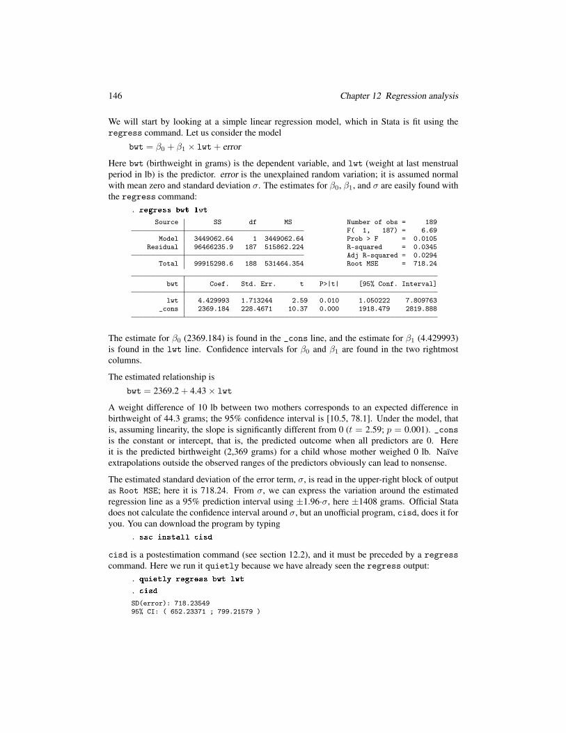
We will start by looking at a simple linear regression model, which in Stata is fit using the

regress command. Let us consider the model

bwt = β0 + β1 × lwt+ error

Here bwt (birthweight in grams) is the dependent variable, and lwt (weight at last menstrual

period in lb) is the predictor. error is the unexplained random variation; it is assumed normal

with mean zero and standard deviation σ. The estimates for β0, β1, and σ are easily found with

the regress command:

. regress bwt lwtSource SS df MS Number of obs = 189

F( 1, 187) = 6.69Model 3449062.64 1 3449062.64 Prob > F = 0.0105

Residual 96466235.9 187 515862.224 R-squared = 0.0345Adj R-squared = 0.0294

Total 99915298.6 188 531464.354 Root MSE = 718.24

bwt Coef. Std. Err. t P>|t| [95% Conf. Interval]

lwt 4.429993 1.713244 2.59 0.010 1.050222 7.809763_cons 2369.184 228.4671 10.37 0.000 1918.479 2819.888

The estimate for β0 (2369.184) is found in the _cons line, and the estimate for β1 (4.429993)

is found in the lwt line. Confidence intervals for β0 and β1 are found in the two rightmost

columns.

The estimated relationship is

bwt = 2369.2 + 4.43 × lwt

A weight difference of 10 lb between two mothers corresponds to an expected difference in

birthweight of 44.3 grams; the 95% confidence interval is [10.5, 78.1]. Under the model, that

is, assuming linearity, the slope is significantly different from 0 (t = 2.59; p = 0.001). _cons

is the constant or intercept, that is, the predicted outcome when all predictors are 0. Here

it is the predicted birthweight (2,369 grams) for a child whose mother weighed 0 lb. Naïve

extrapolations outside the observed ranges of the predictors obviously can lead to nonsense.

The estimated standard deviation of the error term, σ, is read in the upper-right block of output

as Root MSE; here it is 718.24. From σ, we can express the variation around the estimated

regression line as a 95% prediction interval using ±1.96·σ, here ±1408 grams. Official Stata

does not calculate the confidence interval around σ, but an unofficial program, cisd, does it for

you. You can download the program by typing

. ss install isdcisd is a postestimation command (see section 12.2), and it must be preceded by a regress

command. Here we run it quietly because we have already seen the regress output:

. quietly regress bwt lwt

. isdSD(error): 718.2354995% CI: ( 652.23371 ; 799.21579 )

12.1 Linear regression 147

In figure 12.1, a scatterplot with a regression line illustrates the association. You can find a

do-file with the full command (gph_fig12_1.do) at this book’s website, but here we show the

minimum graph command:

. twoway (s atter bwt lwt) (lfit bwt lwt)1000

2000

3000

4000

5000

Birth

we

igh

t (g

ram

s)

50 100 150 200 250

Weight at last menstrual period (lb)

Figure 12.1. Scatterplot with a regression line

We can fit a multiple regression model, that is, a model involving more than one predictor:

bwt = β0 + β1 × lwt+ β2 × age+ error

. regress bwt lwt ageSource SS df MS Number of obs = 189

F( 2, 186) = 3.65Model 3773616.52 2 1886808.26 Prob > F = 0.0279

Residual 96141682.1 186 516890.764 R-squared = 0.0378Adj R-squared = 0.0274

Total 99915298.6 188 531464.354 Root MSE = 718.95

bwt Coef. Std. Err. t P>|t| [95% Conf. Interval]

lwt 4.181336 1.743425 2.40 0.017 .7419072 7.620765age 7.971652 10.06015 0.79 0.429 -11.87501 27.81831

_cons 2216.218 299.2759 7.41 0.000 1625.807 2806.63

From this, we can find the estimated relationship:

bwt = 2216.2 + 4.18 × lwt+ 7.97 × age

The interpretation is that for each pound of maternal prepregnancy weight, the birthweight

increased by 4.18 grams when adjusted for maternal age.

148 Chapter 12 Regression analysis

12.2 Regression postestimation

One of the nice features in Stata is that the default output from a regression analysis is lim-

ited to the most essential information, but afterward, it is possible to supplement an analysis

with additional information, such as calculating diagnostics (residuals, leverages, etc.), testing

specific hypotheses, displaying variance inflation factors, and displaying correlations between

estimates. This is done with postestimation commands, and we will show some examples.

Read about postestimation commands in general in [U] 20 Estimation and postestimation

commands and about specific commands related to regress by typing

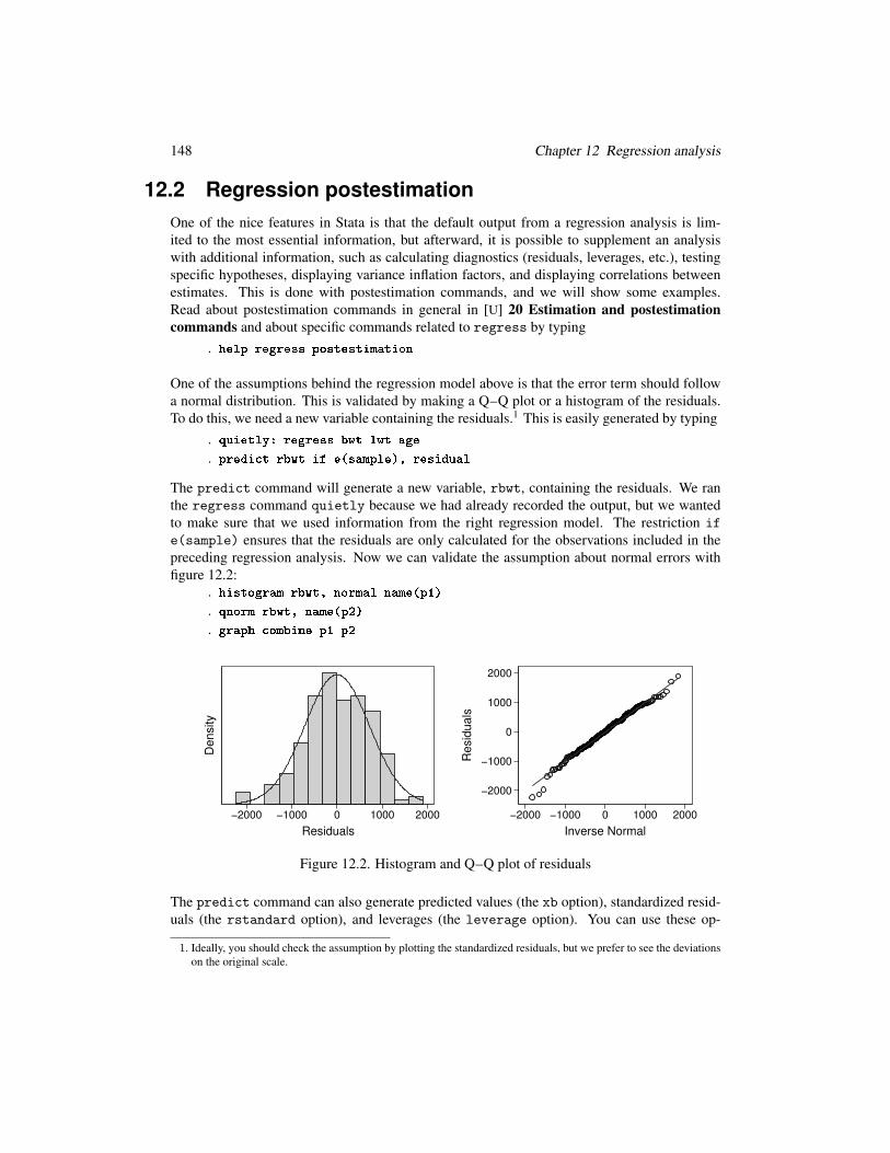
. help regress postestimationOne of the assumptions behind the regression model above is that the error term should follow

a normal distribution. This is validated by making a Q–Q plot or a histogram of the residuals.

To do this, we need a new variable containing the residuals.1 This is easily generated by typing

. quietly: regress bwt lwt age

. predi t rbwt if e(sample), residualThe predict command will generate a new variable, rbwt, containing the residuals. We ran

the regress command quietly because we had already recorded the output, but we wanted

to make sure that we used information from the right regression model. The restriction if

e(sample) ensures that the residuals are only calculated for the observations included in the

preceding regression analysis. Now we can validate the assumption about normal errors with

figure 12.2:

. histogram rbwt, normal name(p1)

. qnorm rbwt, name(p2)

. graph ombine p1 p2

Density

−2000 −1000 0 1000 2000

Residuals

−2000

−1000

0

1000

2000

Resid

uals

−2000 −1000 0 1000 2000

Inverse Normal

Figure 12.2. Histogram and Q–Q plot of residuals

The predict command can also generate predicted values (the xb option), standardized resid-

uals (the rstandard option), and leverages (the leverage option). You can use these op-

1. Ideally, you should check the assumption by plotting the standardized residuals, but we prefer to see the deviations

on the original scale.

12.2 Regression postestimation 149

tions to make diagnostic plots such as “residual versus predicted”, “residuals versus explana-

tory variable”, and “leverage versus residual”, but it is easier to use the postestimation plot

commands that are already in Stata: rvfplot, rvpplot, and lvr2plot; see help regress

postestimation plots. For the above model, we can make the diagnostic plots shown in

figure 12.3 by these commands:

. rvfplot, name(p1) yline(0)

. rvpplot lwt, name(p2) yline(0)

. rvpplot age, name(p3) yline(0)

. lvr2plot, name(p4)

. graph ombine p1 p2 p3 p4−2000

−1000

0

1000

2000

Resid

uals

2600 3100 3600

Fitted values

−2000

−1000

0

1000

2000

Resid

uals

50 100 150 200 250

weight at last menstrual period

−2000

−1000

0

1000

2000

Resid

uals

10 20 30 40 50

age of mother

0

.25

.5

.75

1

Levera

ge

0 .01 .02 .03 .04 .05

Normalized residual squared

Figure 12.3. Diagnostic plots for bwt = β0 + β1×lwt + β2×age + error

None of the first three plots indicates any serious problems with the assumption of linearity.

The leverage-versus-residuals plot shows that no data points have especially high importance

(high leverage) for the results and that no observed bwt differs extremely from the fitted value.

Because figure 12.2 shows only a minor deviation from a normal distribution, we can conclude

that the regression model is appropriate.

Another postestimation command is lincom; it calculates linear combinations of the parameters

in the model. For example, if we want to estimate the expected birthweight of a child born to a

25-year-old woman who weighed 125 lb, that is, β0 + β1 × 125 + β2 × 25, we type

150 Chapter 12 Regression analysis

. lin om _ ons + lwt*125 + age*25( 1) 125*lwt + 25*age + _cons = 0

bwt Coef. Std. Err. t P>|t| [95% Conf. Interval]

(1) 2938.177 56.33194 52.16 0.000 2827.045 3049.308

We could, of course, have found the 2,938.177 by hand, but lincom also supplies a 95% con-

fidence interval. Here the test is of no interest because it evaluates the hypothesis that the

birthweight for a child whose mother weighed 125 lb is 0 grams. If we had wanted to test the

hypothesis that the expected birthweight is 3,000 grams, we could have written

. lin om _ ons + lwt*125 + age*25 - 3000Suppose that we want to estimate the difference in expected birthweight between two babies,

the mother of one of them weighing 15 lb more and being 7 years older than the mother of the

other baby. Doing the calculation by hand, we get 4.18×15+7.97×7 = 118.5 (grams). Using

lincom, we obtain

. lin om lwt*15 + age*7( 1) 15*lwt + 7*age = 0

bwt Coef. Std. Err. t P>|t| [95% Conf. Interval]

(1) 118.5216 70.5696 1.68 0.095 -20.6981 257.7413

The list of postestimation commands also includes test and testparm for testing specific

hypotheses (see the next section for some examples), margins for calculating predictive mar-

gins,2 pwcompare for making pairwise comparisons between levels in a categorical variable,

and estat for calculating the covariance matrix or the correlation matrix of the estimates. It

is a good idea to consult the list of available postestimation commands for the specific type of

model that you want to apply.

12.3 Categorical predictors—factor variables

Until now, we have considered continuous predictors like age and weight, but often we have

categorical predictors, that is, variables that divide observations into categories, such as race:

2. The margins command is very versatile; see Mitchell’s (2012a) Interpreting and Visualizing Regression Models

Using Stata.