Carnegie Mellon

An Introduction to Robot Kinematics

Renata Melamud

Carnegie Mellon

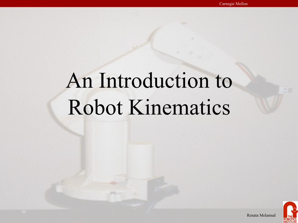
An Example - The PUMA 560

The PUMA 560 has SIX revolute jointsA revolute joint has ONE degree of freedom ( 1 DOF) that is defined by its angle

1

2 3

4

There are two more joints on the end effector (the gripper)

Carnegie Mellon

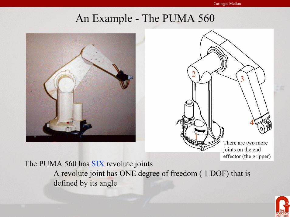
Other basic joints

Spherical Joint3 DOF ( Variables - Υ1, Υ2, Υ3)

Revolute Joint1 DOF ( Variable - Υ)

Prismatic Joint1 DOF (linear) (Variables - d)

Carnegie Mellon

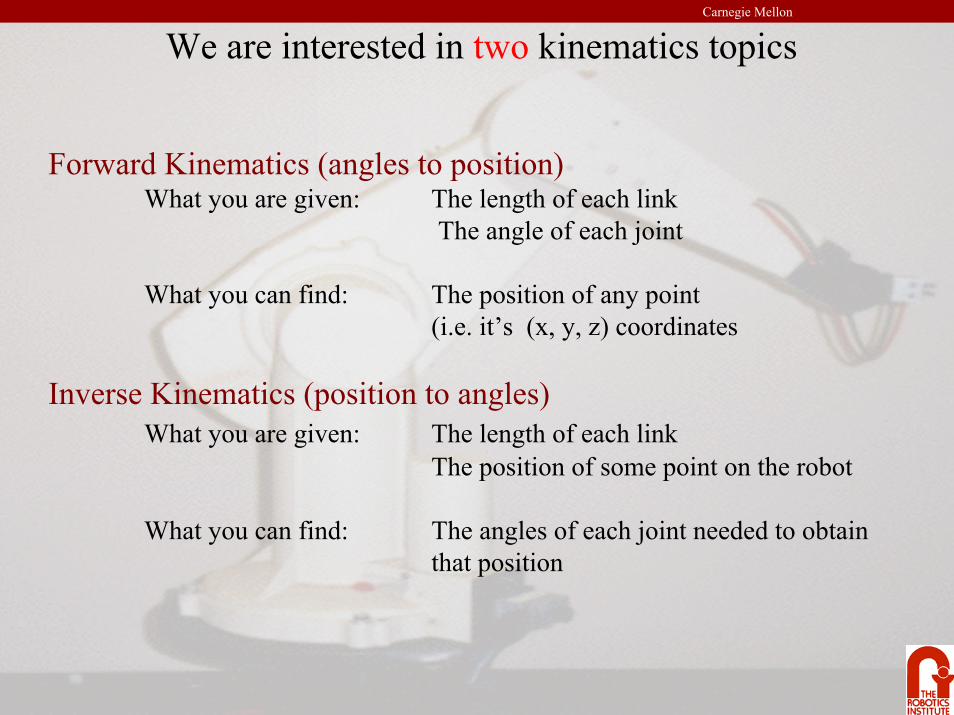
We are interested in two kinematics topics

Forward Kinematics (angles to position)What you are given: The length of each link

The angle of each joint

What you can find: The position of any point(i.e. it’s (x, y, z) coordinates

Inverse Kinematics (position to angles)What you are given: The length of each link

The position of some point on the robot

What you can find: The angles of each joint needed to obtain that position

Carnegie Mellon

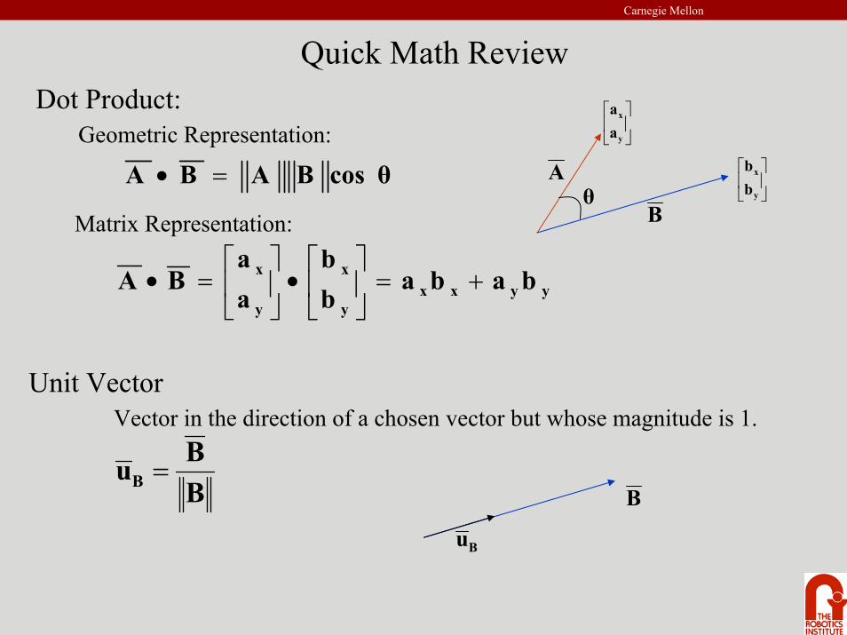
Quick Math ReviewDot Product:

Geometric Representation:A

Bθ

cos θBABA =•

Unit VectorVector in the direction of a chosen vector but whose magnitude is 1.

BBuB =

⎥⎦

⎤⎢⎣

⎡

y

x

aa

Matrix Representation:

⎥⎦

⎤⎢⎣

⎡

y

x

bb

yyxxy

x

y

x bababb

aa

BA +=⎥⎦

⎤⎢⎣

⎡•⎥

⎦

⎤⎢⎣

⎡=•

B

Bu

Carnegie Mellon

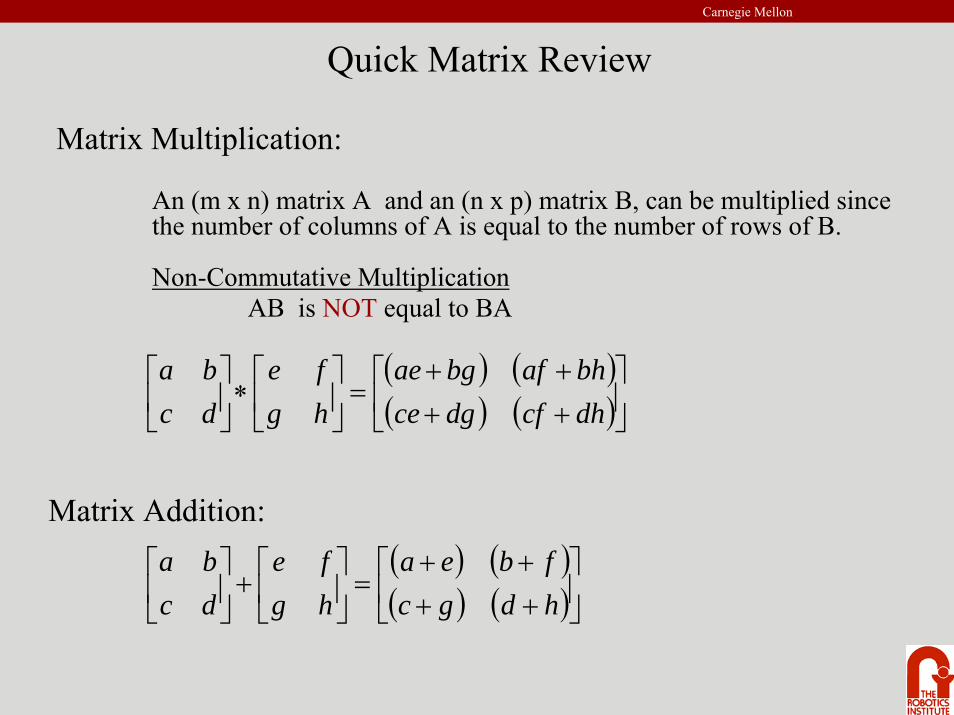
Quick Matrix Review

Matrix Multiplication:

An (m x n) matrix A and an (n x p) matrix B, can be multiplied since the number of columns of A is equal to the number of rows of B.

Non-Commutative MultiplicationAB is NOT equal to BA

( ) ( )( ) ( )⎥⎦

⎤⎢⎣

⎡++++

=⎥⎦

⎤⎢⎣

⎡∗⎥⎦

⎤⎢⎣

⎡dhcfdgcebhafbgae

hgfe

dcba

Matrix Addition:( ) ( )( ) ( )⎥⎦

⎤⎢⎣

⎡++++

=⎥⎦

⎤⎢⎣

⎡+⎥

⎦

⎤⎢⎣

⎡hdgcfbea

hgfe

dcba

Carnegie Mellon

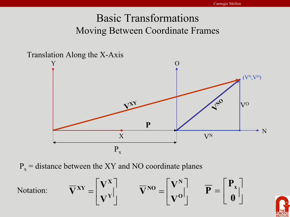
Basic TransformationsMoving Between Coordinate Frames

Translation Along the X-Axis

N

OY

VNO

VXY

X

Px

VN

VO

Px = distance between the XY and NO coordinate planes

⎥⎦

⎤⎢⎣

⎡= Y

XXY

VV

V ⎥⎦

⎤⎢⎣

⎡= O

NNO

VV

V ⎥⎦

⎤⎢⎣

⎡=

0P

P x

P

(VN,VO)

Notation:

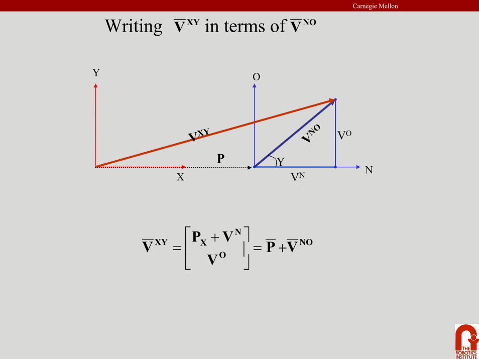
Carnegie Mellon

NX

VNO

VXY

PVN

VO

OY

Υ

NOO

NXXY VPV

VPV +=⎥

⎦

⎤⎢⎣

⎡ +=

Writing in terms of XYV NOV

Carnegie Mellon

X

VXY

PXY

N

VNO

VN

VO

Y

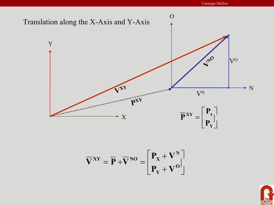
OTranslation along the X-Axis and Y-Axis

⎥⎦

⎤⎢⎣

⎡

++

=+= OY

NXNOXY

VPVP

VPV

⎥⎦

⎤⎢⎣

⎡=

Y

xXY

PP

P

Carnegie Mellon

⎥⎦

⎤⎢⎣

⎡

••

=⎥⎥⎦

⎤

⎢⎢⎣

⎡

−=

⎥⎥⎦

⎤

⎢⎢⎣

⎡=⎥

⎦

⎤⎢⎣

⎡=

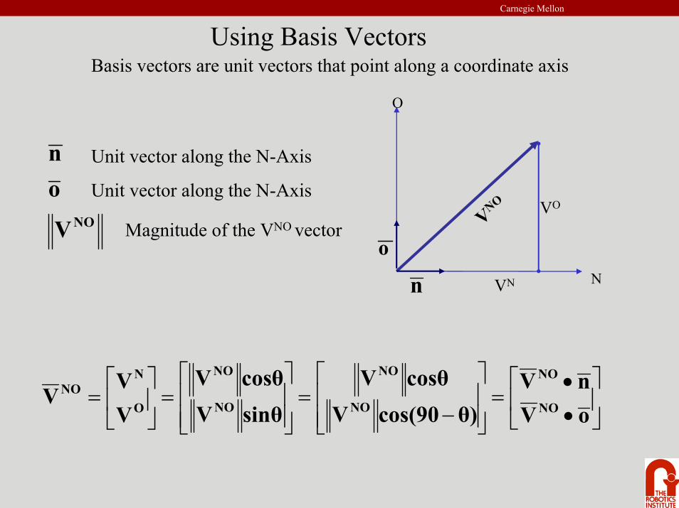
oVnV

θ)cos(90VcosθV

sinθVcosθV

VV

V NO

NO

NO

NO

NO

NO

O

NNO

NOV

on Unit vector along the N-Axis

Unit vector along the N-Axis

Magnitude of the VNO vector

Using Basis VectorsBasis vectors are unit vectors that point along a coordinate axis

N

VNO

VN

VO

O

n

o

Carnegie Mellon

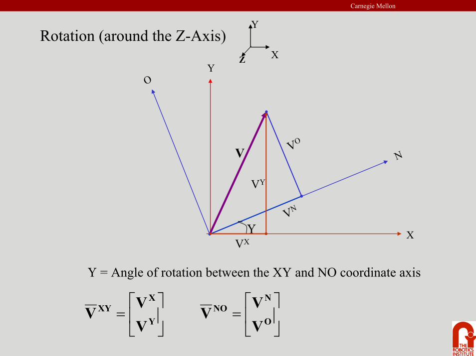
Rotation (around the Z-Axis)X

Y

Z

X

Y

N

VN

VO

O

Υ

V

VX

VY

⎥⎦

⎤⎢⎣

⎡= Y

XXY

VV

V ⎥⎦

⎤⎢⎣

⎡= O

NNO

VV

V

Υ = Angle of rotation between the XY and NO coordinate axis

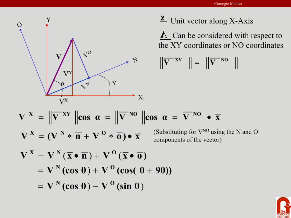
Carnegie Mellon

X

Y

N

VN

VO

O

Υ

V

VX

VY

α

Unit vector along X-Axis

xxVcos αVcos αVV NONOXYX •===

NOXY VV =

Can be considered with respect to the XY coordinates or NO coordinates

Vx)oVn(VV ONX •∗+∗= (Substituting for VNO using the N and O

components of the vector)

)oxVnxVV ONX •+•= ()(

)))

(sin θV(cos θV90))(cos( θV(cos θV

ON

ON

−=

++=

Carnegie Mellon

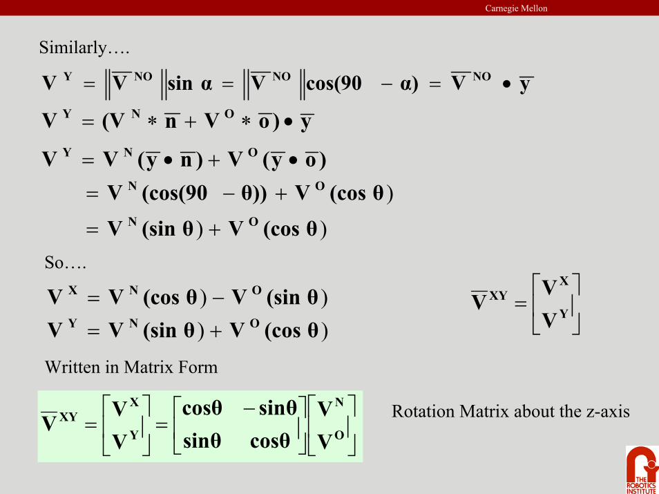
Similarly….

yVα)cos(90Vsin αVV NONONOY •=−==

y)oVn(VV ONY •∗+∗=

)oy(V)ny(VV ONY •+•=

)))

(cos θV(sin θV(cos θVθ))(cos(90V

ON

ON

+=

+−=

So….

)) (cos θV(sin θVV ONY +=)) (sin θV(cos θVV ONX −= ⎥

⎦

⎤⎢⎣

⎡= Y

XXY

VV

V

Written in Matrix Form

⎥⎦

⎤⎢⎣

⎡⎥⎦

⎤⎢⎣

⎡ −=⎥

⎦

⎤⎢⎣

⎡=

O

N

Y

XXY

VV

cosθsinθsinθcosθ

VV

V Rotation Matrix about the z-axis

Carnegie Mellon

X1

Y1

N

O

ΥVXY

X0

Y0

VNO

P

(VN,VO)

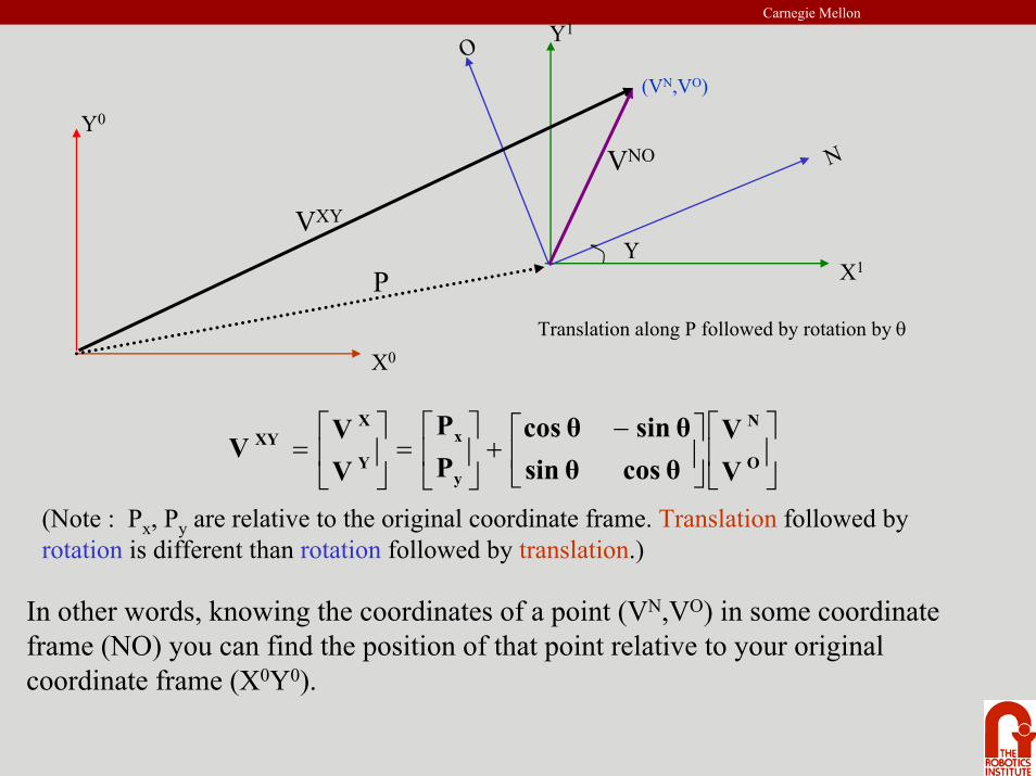
Translation along P followed by rotation by θ

⎥⎦

⎤⎢⎣

⎡⎥⎦

⎤⎢⎣

⎡ −+⎥

⎦

⎤⎢⎣

⎡=⎥

⎦

⎤⎢⎣

⎡=

O

N

y

xY

XXY

VV

cos θsin θsin θcos θ

PP

VV

V

In other words, knowing the coordinates of a point (VN,VO) in some coordinate frame (NO) you can find the position of that point relative to your original coordinate frame (X0Y0).

(Note : Px, Py are relative to the original coordinate frame. Translation followed by rotation is different than rotation followed by translation.)

Carnegie Mellon

⎥⎦

⎤⎢⎣

⎡⎥⎦

⎤⎢⎣

⎡ −+⎥

⎦

⎤⎢⎣

⎡=⎥

⎦

⎤⎢⎣

⎡=

O

N

y

xY

XXY

VV

cos θsin θsin θcos θ

PP

VV

V

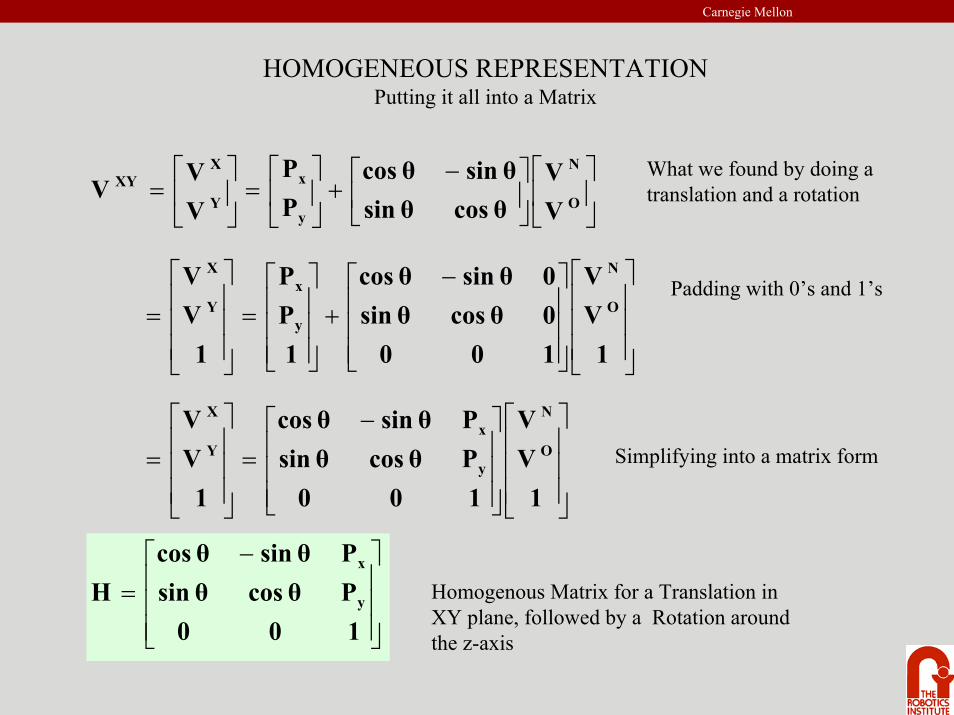
HOMOGENEOUS REPRESENTATIONPutting it all into a Matrix

⎥⎥⎥

⎦

⎤

⎢⎢⎢

⎣

⎡

⎥⎥⎥

⎦

⎤

⎢⎢⎢

⎣

⎡ −+

⎥⎥⎥

⎦

⎤

⎢⎢⎢

⎣

⎡=

⎥⎥⎥

⎦

⎤

⎢⎢⎢

⎣

⎡

=1

VV

1000cos θsin θ0sin θcos θ

1PP

1VV

O

N

y

xY

X

⎥⎥⎥

⎦

⎤

⎢⎢⎢

⎣

⎡

⎥⎥⎥

⎦

⎤

⎢⎢⎢

⎣

⎡ −=

⎥⎥⎥

⎦

⎤

⎢⎢⎢

⎣

⎡

=1

VV

100Pcos θsin θPsin θcos θ

1VV

O

N

y

xY

X

What we found by doing a translation and a rotation

Padding with 0’s and 1’s

Simplifying into a matrix form

⎥⎥⎥

⎦

⎤

⎢⎢⎢

⎣

⎡ −=

100Pcos θsin θPsin θcos θ

H y

x

Homogenous Matrix for a Translation in XY plane, followed by a Rotation around the z-axis

Carnegie Mellon

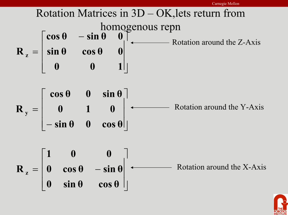
Rotation Matrices in 3D – OK,lets return from homogenous repn

⎥⎥⎥

⎦

⎤

⎢⎢⎢

⎣

⎡ −=

1000cos θsin θ0sin θcos θ

R z

Rotation around the Z-Axis

⎥⎥⎥

⎦

⎤

⎢⎢⎢

⎣

⎡

−=

cos θ0sin θ010

sin θ0cos θR y

⎥⎥⎥

⎦

⎤

⎢⎢⎢

⎣

⎡−=cos θsin θ0sin θcos θ0001

R z

Rotation around the Y-Axis

Rotation around the X-Axis

Carnegie Mellon

⎥⎥⎥⎥

⎦

⎤

⎢⎢⎢⎢

⎣

⎡

=

10000aon0aon0aon

Hzzz

yyy

xxx

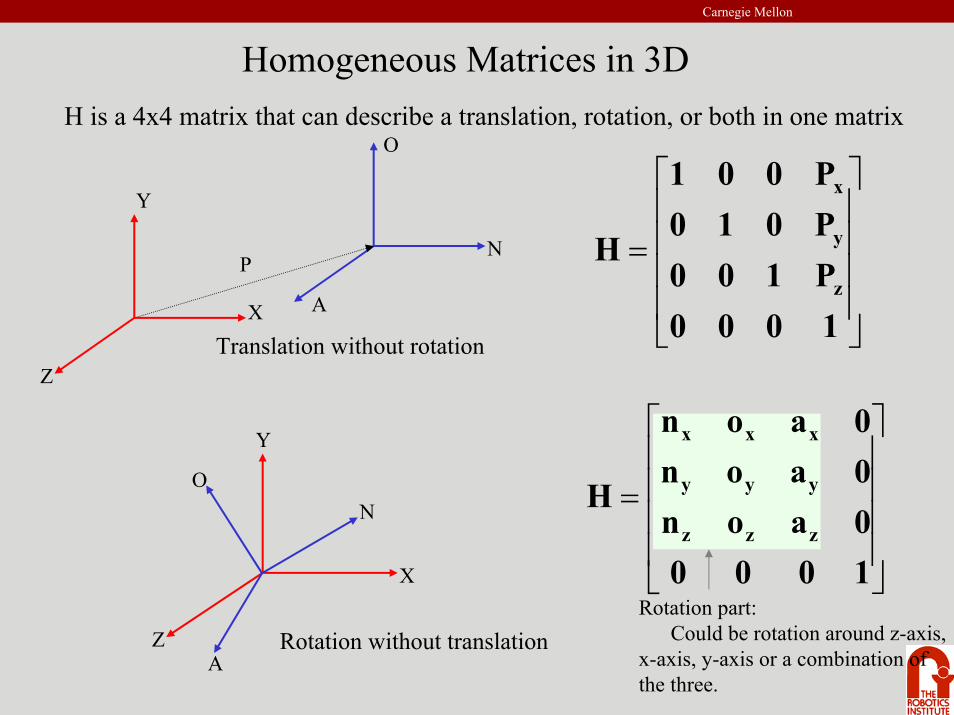
Homogeneous Matrices in 3DH is a 4x4 matrix that can describe a translation, rotation, or both in one matrix

Translation without rotation⎥⎥⎥⎥

⎦

⎤

⎢⎢⎢⎢

⎣

⎡

=

1000P100P010P001

Hz

y

x

P

Y

X

Z

O

N

A

Y

X

Z

ON

ARotation without translation

Rotation part:Could be rotation around z-axis,

x-axis, y-axis or a combination of the three.

Carnegie Mellon

⎥⎥⎥⎥⎥

⎦

⎤

⎢⎢⎢⎢⎢

⎣

⎡

=

1

A

O

N

XY

VVV

HV

⎥⎥⎥⎥⎥

⎦

⎤

⎢⎢⎢⎢⎢

⎣

⎡

⎥⎥⎥⎥

⎦

⎤

⎢⎢⎢⎢

⎣

⎡

=

1

A

O

N

zzzz

yyyy

xxxx

XY

VVV

1000PaonPaonPaon

V

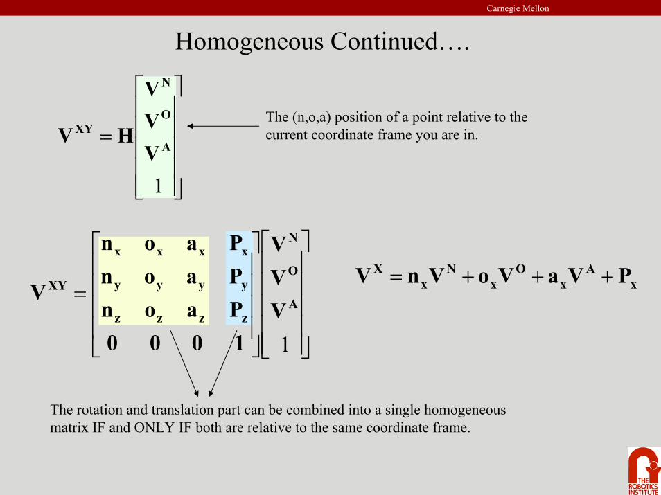
Homogeneous Continued….

The (n,o,a) position of a point relative to the current coordinate frame you are in.

The rotation and translation part can be combined into a single homogeneous matrix IF and ONLY IF both are relative to the same coordinate frame.

xA

xO

xN

xX PVaVoVnV +++=

Carnegie Mellon

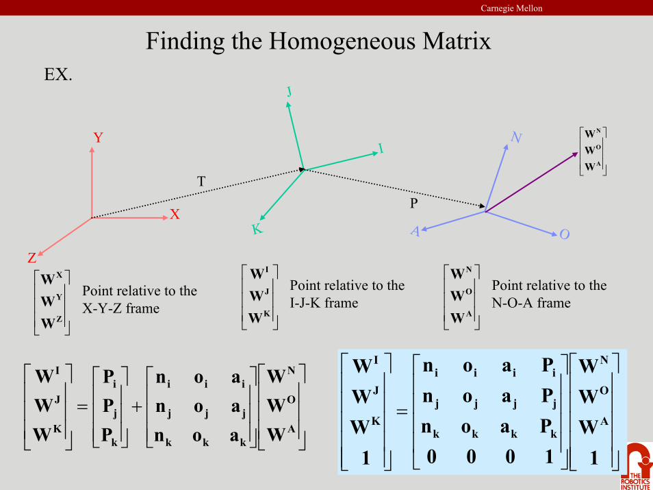
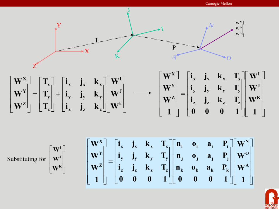
Finding the Homogeneous MatrixEX.

Y

X

Z

J

I

K

N

OA

TP

⎥⎥⎥

⎦

⎤

⎢⎢⎢

⎣

⎡

A

O

N

WWW

⎥⎥⎥

⎦

⎤

⎢⎢⎢

⎣

⎡

A

O

N

WWW

⎥⎥⎥

⎦

⎤

⎢⎢⎢

⎣

⎡

K

J

I

WWW

⎥⎥⎥

⎦

⎤

⎢⎢⎢

⎣

⎡

Z

Y

X

WWW Point relative to the

N-O-A framePoint relative to theX-Y-Z frame

Point relative to theI-J-K frame

⎥⎥⎥

⎦

⎤

⎢⎢⎢

⎣

⎡

⎥⎥⎥

⎦

⎤

⎢⎢⎢

⎣

⎡+

⎥⎥⎥

⎦

⎤

⎢⎢⎢

⎣

⎡=

⎥⎥⎥

⎦

⎤

⎢⎢⎢

⎣

⎡

A

O

N

kkk

jjj

iii

k

j

i

K

J

I

WWW

aonaonaon

PPP

WWW

⎥⎥⎥⎥⎥

⎦

⎤

⎢⎢⎢⎢⎢

⎣

⎡

⎥⎥⎥⎥

⎦

⎤

⎢⎢⎢⎢

⎣

⎡

=

⎥⎥⎥⎥⎥

⎦

⎤

⎢⎢⎢⎢⎢

⎣

⎡

1WWW

1000PaonPaonPaon

1WWW

A

O

N

kkkk

jjjj

iiii

K

J

I

Carnegie Mellon

Y

X

Z

J

I

K

N

OA

TP

⎥⎥⎥

⎦

⎤

⎢⎢⎢

⎣

⎡

A

O

N

WWW

⎥⎥⎥

⎦

⎤

⎢⎢⎢

⎣

⎡

⎥⎥⎥

⎦

⎤

⎢⎢⎢

⎣

⎡+

⎥⎥⎥

⎦

⎤

⎢⎢⎢

⎣

⎡=

⎥⎥⎥

⎦

⎤

⎢⎢⎢

⎣

⎡

k

J

I

zzz

yyy

xxx

z

y

x

Z

Y

X

WWW

kjikjikji

TTT

WWW

⎥⎥⎥⎥⎥

⎦

⎤

⎢⎢⎢⎢⎢

⎣

⎡

⎥⎥⎥⎥

⎦

⎤

⎢⎢⎢⎢

⎣

⎡

=

⎥⎥⎥⎥⎥

⎦

⎤

⎢⎢⎢⎢⎢

⎣

⎡

1WWW

1000TkjiTkjiTkji

1WWW

K

J

I

zzzz

yyyy

xxxx

Z

Y

X

Substituting for⎥⎥⎥

⎦

⎤

⎢⎢⎢

⎣

⎡

K

J

I

WWW

⎥⎥⎥⎥⎥

⎦

⎤

⎢⎢⎢⎢⎢

⎣

⎡

⎥⎥⎥⎥

⎦

⎤

⎢⎢⎢⎢

⎣

⎡

⎥⎥⎥⎥

⎦

⎤

⎢⎢⎢⎢

⎣

⎡

=

⎥⎥⎥⎥⎥

⎦

⎤

⎢⎢⎢⎢⎢

⎣

⎡

1WWW

1000PaonPaonPaon

1000TkjiTkjiTkji

1WWW

A

O

N

kkkk

jjjj

iiii

zzzz

yyyy

xxxx

Z

Y

X

Carnegie Mellon

⎥⎥⎥⎥⎥

⎦

⎤

⎢⎢⎢⎢⎢

⎣

⎡

=

⎥⎥⎥⎥⎥

⎦

⎤

⎢⎢⎢⎢⎢

⎣

⎡

1WWW

H

1WWW

A

O

N

Z

Y

X

⎥⎥⎥⎥

⎦

⎤

⎢⎢⎢⎢

⎣

⎡

⎥⎥⎥⎥

⎦

⎤

⎢⎢⎢⎢

⎣

⎡

=

1000PaonPaonPaon

1000TkjiTkjiTkji

Hkkkk

jjjj

iiii

zzzz

yyyy

xxxx

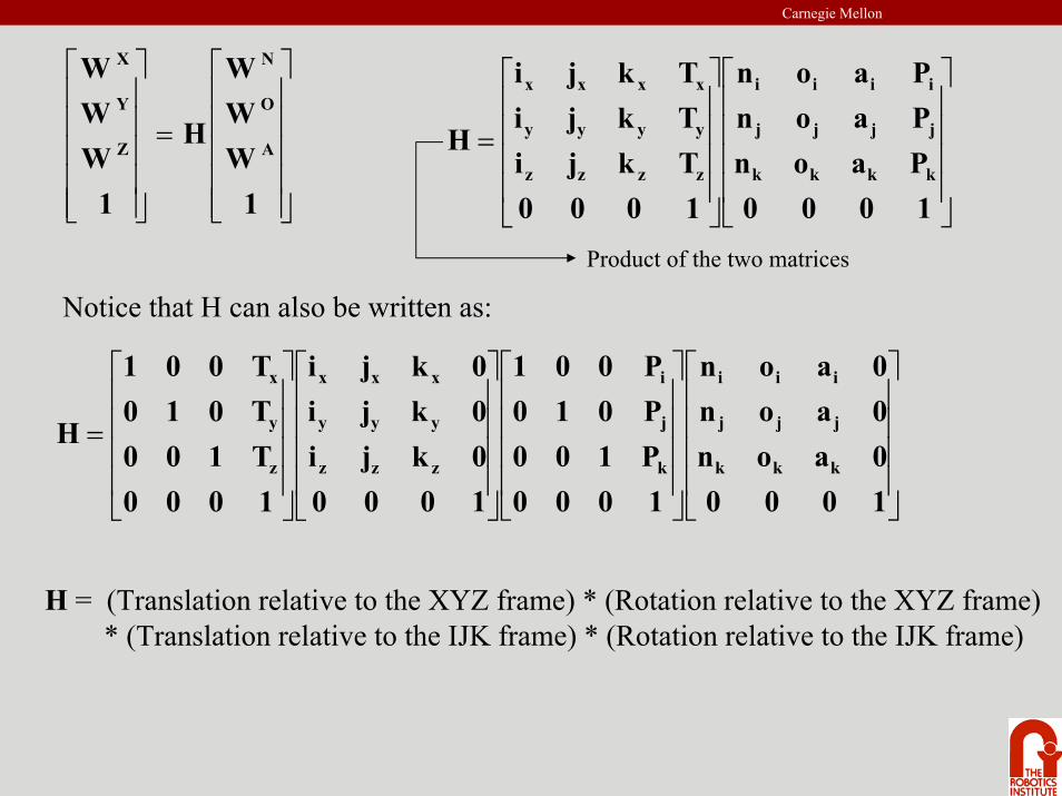
Product of the two matrices

Notice that H can also be written as:

⎥⎥⎥⎥

⎦

⎤

⎢⎢⎢⎢

⎣

⎡

⎥⎥⎥⎥

⎦

⎤

⎢⎢⎢⎢

⎣

⎡

⎥⎥⎥⎥

⎦

⎤

⎢⎢⎢⎢

⎣

⎡

⎥⎥⎥⎥

⎦

⎤

⎢⎢⎢⎢

⎣

⎡

=

10000aon0aon0aon

1000P100P010P001

10000kji0kji0kji

1000T100T010T001

Hkkk

jjj

iii

k

j

i

zzz

yyy

xxx

z

y

x

H = (Translation relative to the XYZ frame) * (Rotation relative to the XYZ frame) * (Translation relative to the IJK frame) * (Rotation relative to the IJK frame)

Carnegie Mellon

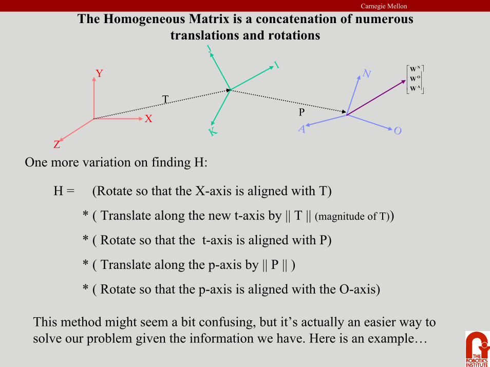
The Homogeneous Matrix is a concatenation of numerous translations and rotations

Y

X

Z

JI

K

N

OA

TP

⎥⎥⎥

⎦

⎤

⎢⎢⎢

⎣

⎡

A

O

N

WWW

One more variation on finding H:

H = (Rotate so that the X-axis is aligned with T)

* ( Translate along the new t-axis by || T || (magnitude of T))

* ( Rotate so that the t-axis is aligned with P)

* ( Translate along the p-axis by || P || )

* ( Rotate so that the p-axis is aligned with the O-axis)

This method might seem a bit confusing, but it’s actually an easier way to solve our problem given the information we have. Here is an example…

Carnegie Mellon

F o r w a r d K i n e m a t i c s

Carnegie Mellon

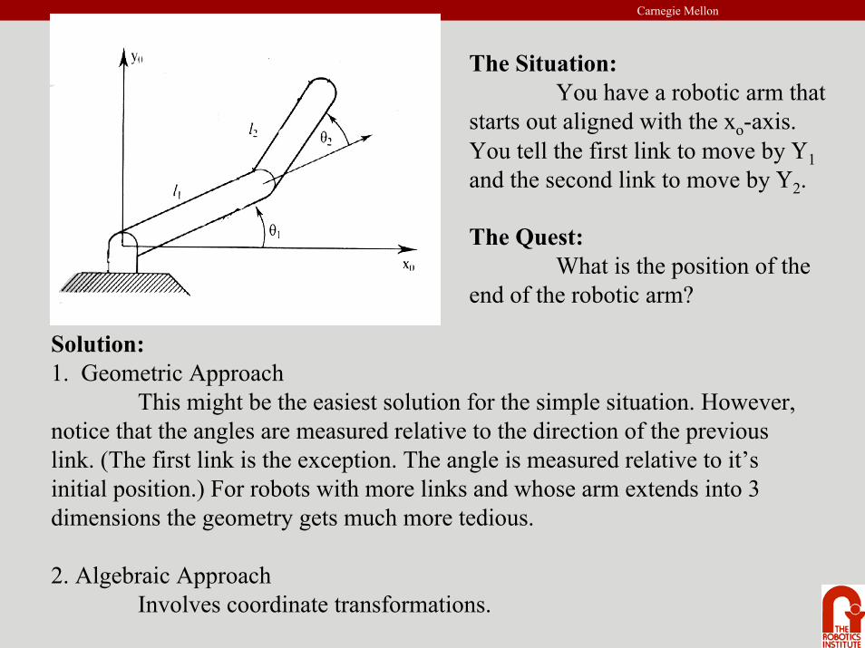
The Situation:You have a robotic arm that

starts out aligned with the xo-axis.You tell the first link to move by Υ1and the second link to move by Υ2.

The Quest:What is the position of the

end of the robotic arm?

Solution:1. Geometric Approach

This might be the easiest solution for the simple situation. However, notice that the angles are measured relative to the direction of the previous link. (The first link is the exception. The angle is measured relative to it’s initial position.) For robots with more links and whose arm extends into 3 dimensions the geometry gets much more tedious.

2. Algebraic Approach Involves coordinate transformations.

Carnegie Mellon

X2

X3Y2

Y3

Υ1

Υ2

Υ3

1

2 3

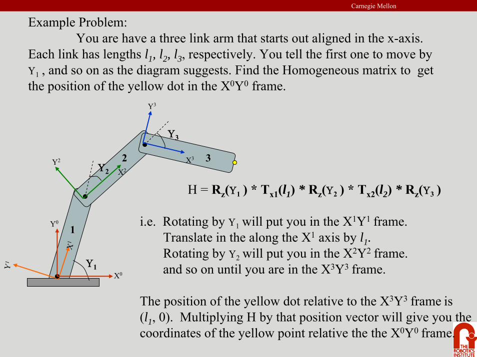
H = Rz(Υ1 ) * Tx1(l1) * Rz(Υ2 ) * Tx2(l2) * Rz(Υ3 )

i.e. Rotating by Υ1 will put you in the X1Y1 frame.Translate in the along the X1 axis by l1.Rotating by Υ2 will put you in the X2Y2 frame.and so on until you are in the X3Y3 frame.

The position of the yellow dot relative to the X3Y3 frame is(l1, 0). Multiplying H by that position vector will give you the coordinates of the yellow point relative the the X0Y0 frame.

Example Problem: You are have a three link arm that starts out aligned in the x-axis.

Each link has lengths l1, l2, l3, respectively. You tell the first one to move by Υ1 , and so on as the diagram suggests. Find the Homogeneous matrix to get the position of the yellow dot in the X0Y0 frame.

X1

Y1

X0

Y0

Carnegie Mellon

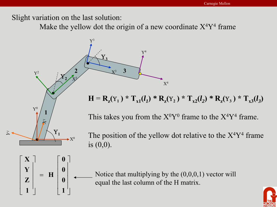
Slight variation on the last solution:Make the yellow dot the origin of a new coordinate X4Y4 frame

X2

X3Y2

Y3

Υ1

Υ2

Υ3

1

2 3

X1

Y1

X0

Y0

X4

Y4

H = Rz(Υ1 ) * Tx1(l1) * Rz(Υ2 ) * Tx2(l2) * Rz(Υ3 ) * Tx3(l3)

This takes you from the X0Y0 frame to the X4Y4 frame.

The position of the yellow dot relative to the X4Y4 frame is (0,0).

⎥⎥⎥⎥

⎦

⎤

⎢⎢⎢⎢

⎣

⎡

=

⎥⎥⎥⎥

⎦

⎤

⎢⎢⎢⎢

⎣

⎡

1000

H

1ZYX

Notice that multiplying by the (0,0,0,1) vector will equal the last column of the H matrix.

Carnegie Mellon

More on Forward Kinematics…

Denavit - Hartenberg Parameters

Carnegie Mellon

Denavit-Hartenberg Notation

Z(i - 1)

X(i -1)

Y(i -1)

α( i - 1)

a(i - 1 )

Z i Y i

X i a i d i

Υ i

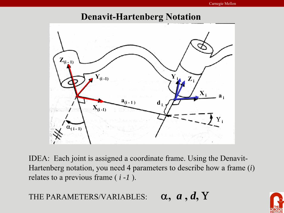
IDEA: Each joint is assigned a coordinate frame. Using the Denavit-Hartenberg notation, you need 4 parameters to describe how a frame (i) relates to a previous frame ( i -1 ).

THE PARAMETERS/VARIABLES: α, a , d, Υ

Carnegie Mellon

The Parameters

Z(i - 1)

X(i -1)

Y(i -1)

α( i - 1)

a(i - 1 )

Z i Y i

X i a i d i

Υ i

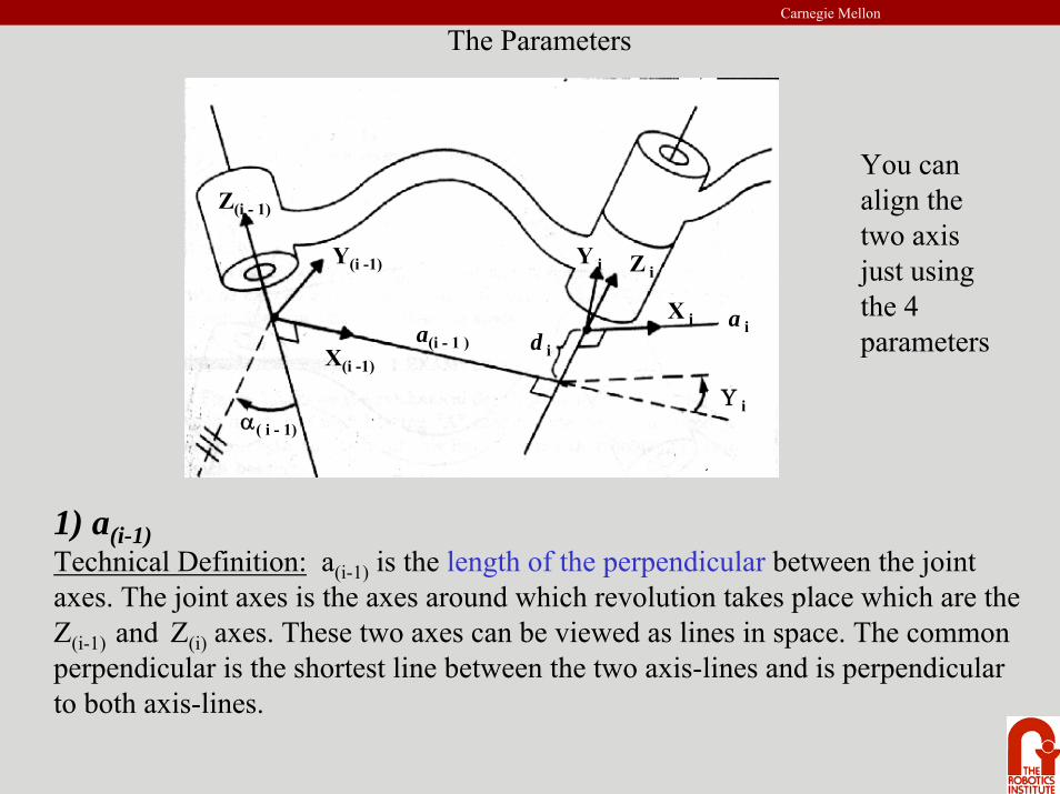
You can align the two axis just using the 4 parameters

1) a(i-1)Technical Definition: a(i-1) is the length of the perpendicular between the joint axes. The joint axes is the axes around which revolution takes place which are the Z(i-1) and Z(i) axes. These two axes can be viewed as lines in space. The common perpendicular is the shortest line between the two axis-lines and is perpendicular to both axis-lines.

Carnegie Mellon

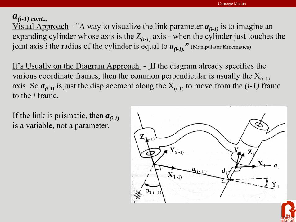
a(i-1) cont...Visual Approach - “A way to visualize the link parameter a(i-1) is to imagine an expanding cylinder whose axis is the Z(i-1) axis - when the cylinder just touches the joint axis i the radius of the cylinder is equal to a(i-1).” (Manipulator Kinematics)

It’s Usually on the Diagram Approach - If the diagram already specifies the various coordinate frames, then the common perpendicular is usually the X(i-1)axis. So a(i-1) is just the displacement along the X(i-1) to move from the (i-1) frame to the i frame.

If the link is prismatic, then a(i-1)is a variable, not a parameter.

Z(i - 1)

X(i -1)

Y(i -1)

α( i - 1)

a(i - 1 )

Z i Y i

X i a i d i

Υ i

Carnegie Mellon

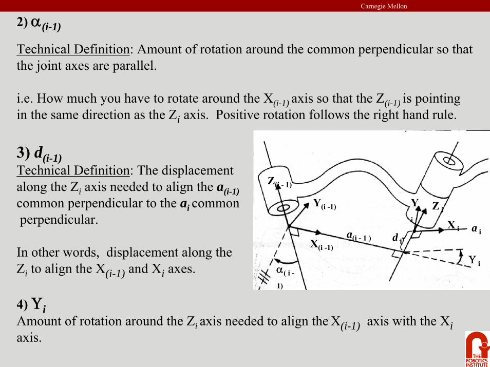
2) α(i-1)

Technical Definition: Amount of rotation around the common perpendicular so that the joint axes are parallel.

i.e. How much you have to rotate around the X(i-1) axis so that the Z(i-1) is pointing in the same direction as the Zi axis. Positive rotation follows the right hand rule.

3) d(i-1)Technical Definition: The displacement along the Zi axis needed to align the a(i-1)common perpendicular to the ai commonperpendicular.

In other words, displacement along the Zi to align the X(i-1) and Xi axes.

4) Υi Amount of rotation around the Zi axis needed to align the X(i-1) axis with the Xiaxis.

Z(i - 1)

X(i -1)

Y(i -1)

α( i -

1)

a(i - 1 )

Z i Yi X i a i d i

Υ i

Carnegie Mellon

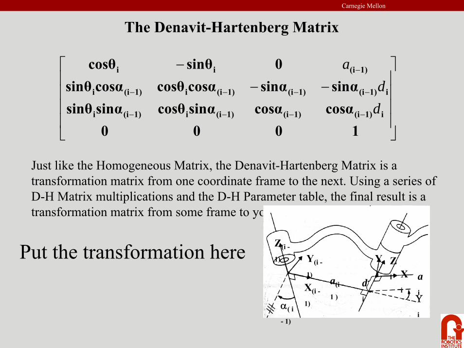
The Denavit-Hartenberg Matrix

⎥⎥⎥⎥

⎦

⎤

⎢⎢⎢⎢

⎣

⎡−−

−

−−−−

−−−−

−

1000cosαcosαsinαcosθsinαsinθsinαsinαcosαcosθcosαsinθ

0sinθcosθ

i1)(i1)(i1)(ii1)(ii

i1)(i1)(i1)(ii1)(ii

1)(iii

dd

a

Just like the Homogeneous Matrix, the Denavit-Hartenberg Matrix is a transformation matrix from one coordinate frame to the next. Using a series of D-H Matrix multiplications and the D-H Parameter table, the final result is a transformation matrix from some frame to your initial frame.

Z(i -

1)

X(i -

1)

Y(i -

1)

α( i

- 1)

a(i -

1 )

Zi

Yi X

i

ai

di Υ

i

Put the transformation here

Carnegie Mellon

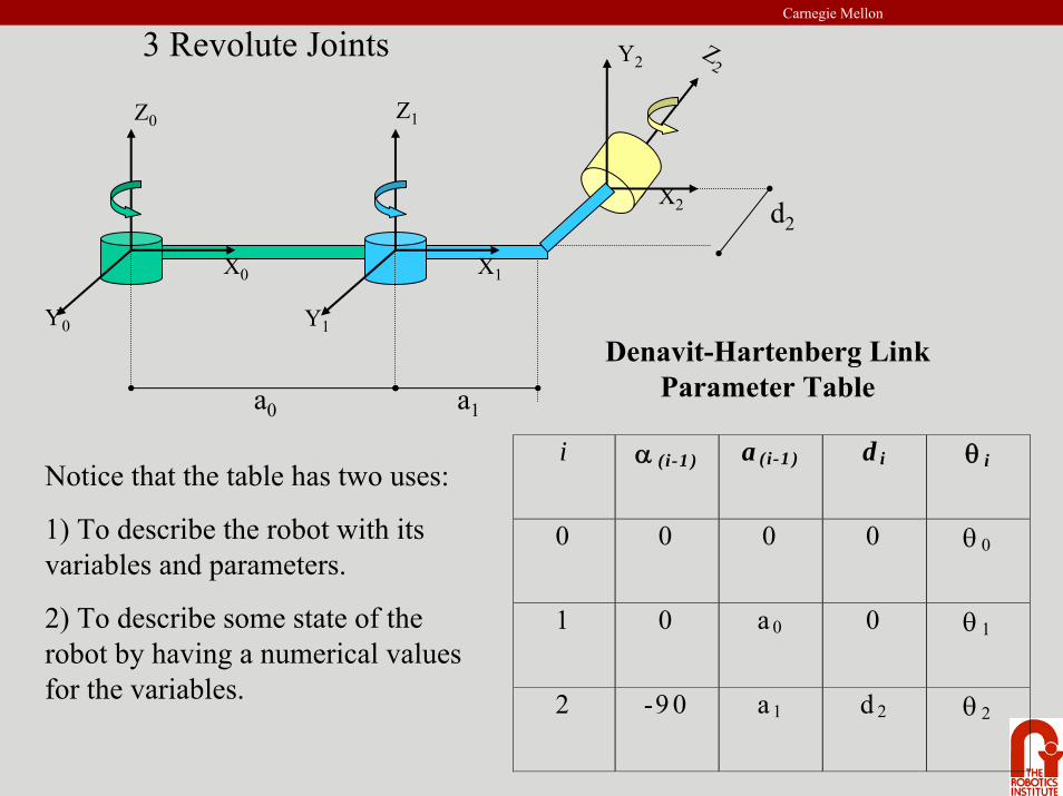
3 Revolute Joints

i α (i-1 ) a (i-1 ) d i θ i

0 0 0 0 θ 0

1 0 a 0 0 θ 1

2 -9 0 a 1 d 2 θ 2

Z0

X0

Y0

Z1

X2

Y1

Z2

X1

Y2

d2

a0 a1

Denavit-Hartenberg Link Parameter Table

Notice that the table has two uses:

1) To describe the robot with its variables and parameters.

2) To describe some state of the robot by having a numerical values for the variables.

Carnegie Mellon

Z0

X0

Y0

Z1

X2

Y1

Z2

X1

Y2

d2

a0 a1

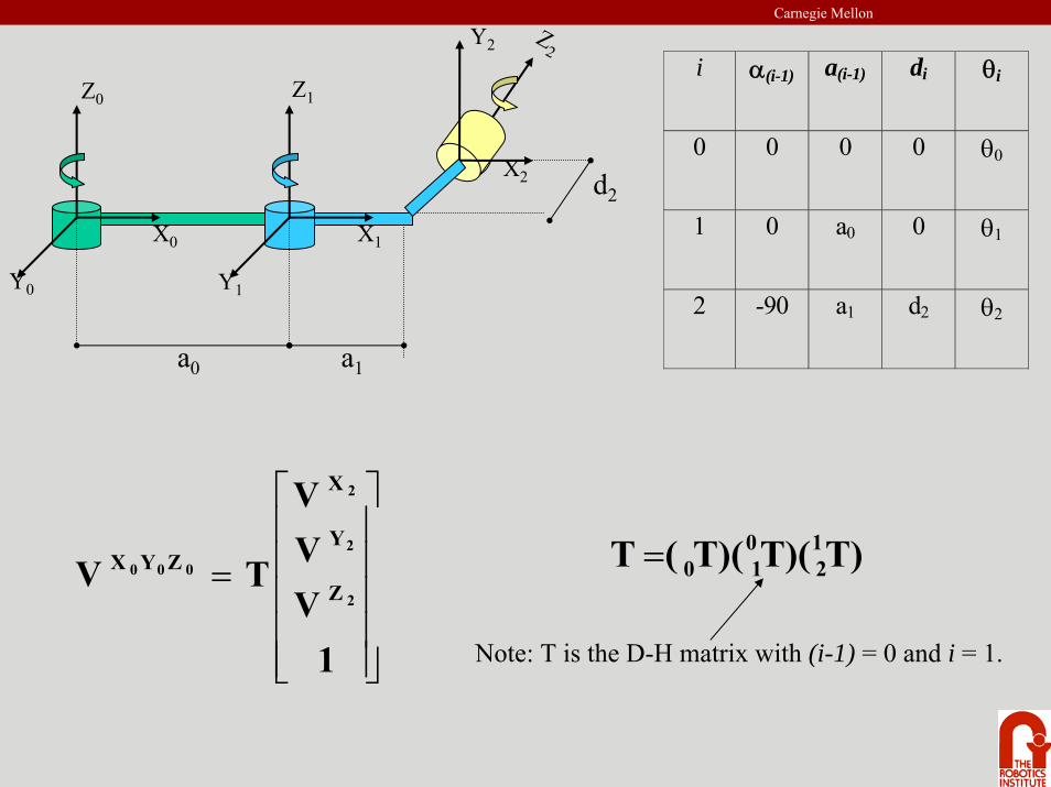
i α(i-1) a(i-1) di θi

0 0 0 0 θ0

1 0 a0 0 θ1

2 -90 a1 d2 θ2

⎥⎥⎥⎥⎥

⎦

⎤

⎢⎢⎢⎢⎢

⎣

⎡

=

1VVV

TV2

2

2

000

Z

Y

X

ZYX T)T)(T)((T 12

010=

Note: T is the D-H matrix with (i-1) = 0 and i = 1.

Carnegie Mellon

⎥⎥⎥⎥

⎦

⎤

⎢⎢⎢⎢

⎣

⎡ −

=

1000010000cosθsinθ00sinθcosθ

T 00

00

0

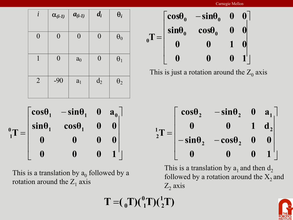
i α(i-1) a(i-1) di θi

0 0 0 0 θ0

1 0 a0 0 θ1

2 -90 a1 d2 θ2

⎥⎥⎥⎥

⎦

⎤

⎢⎢⎢⎢

⎣

⎡ −

=

1000000000cosθsinθa0sinθcosθ

T 11

011

01

This is just a rotation around the Z0 axis

⎥⎥⎥⎥

⎦

⎤

⎢⎢⎢⎢

⎣

⎡

−−

−

=

100000cosθsinθ

d100a0sinθcosθ

T22

2

122

12

This is a translation by a0 followed by a rotation around the Z1 axis

This is a translation by a1 and then d2followed by a rotation around the X2 andZ2 axis

T)T)(T)((T 12

010=

Carnegie Mellon

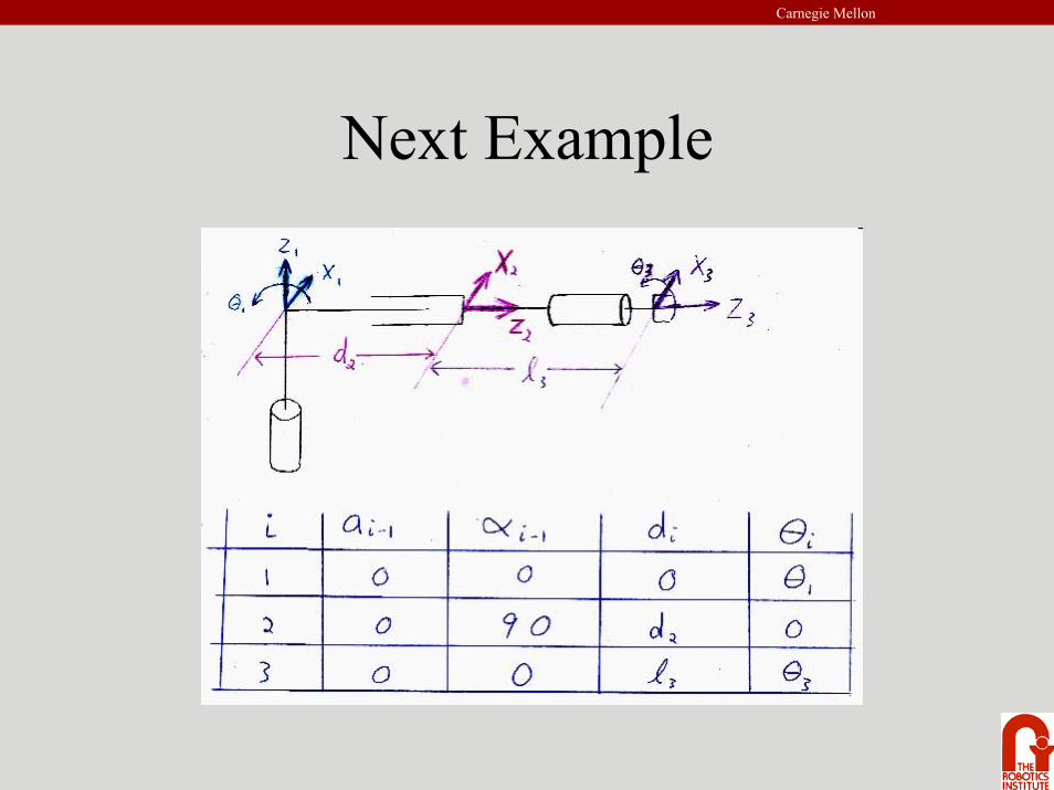
Next Example

Carnegie Mellon

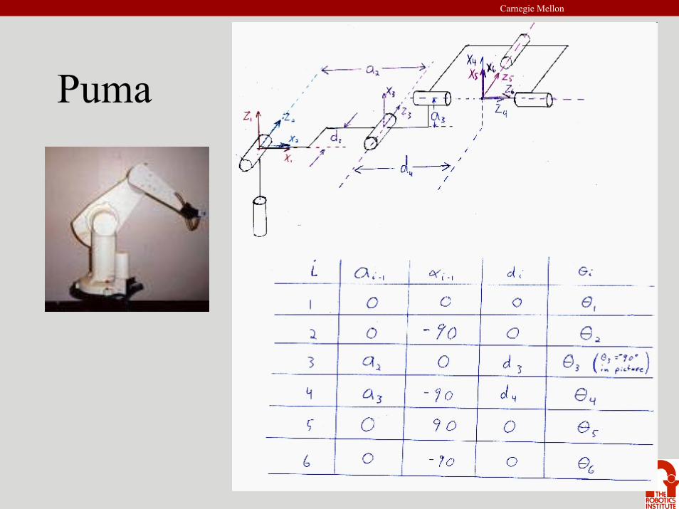
Puma

Carnegie Mellon

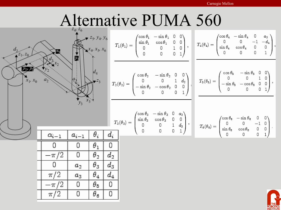
Alternative PUMA 560

Carnegie Mellon

I n v e r s e K i n e m a t i c s

From Position to Angles

Carnegie Mellon

A Simple Example

Υ1

X

Y

S

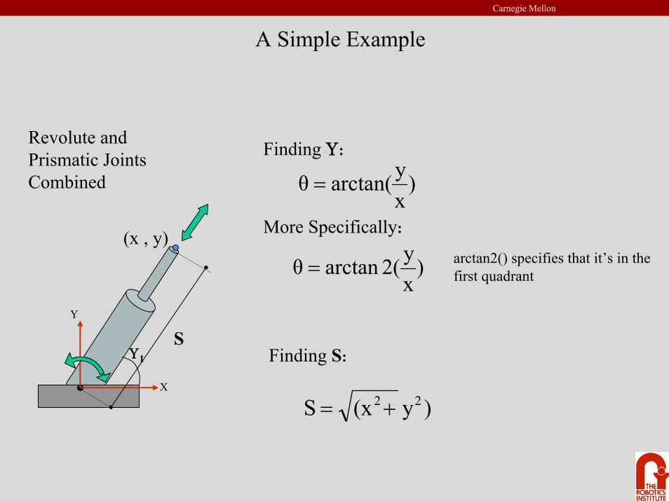
Revolute and Prismatic Joints Combined

(x , y)

Finding Υ:

)xyarctan(θ =

More Specifically:

)xy(2arctanθ = arctan2() specifies that it’s in the

first quadrant

Finding S:

)y(xS 22+=

Carnegie Mellon

Υ2

Υ1

(x , y)

l2

l1

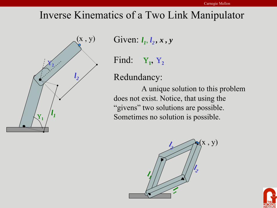
Inverse Kinematics of a Two Link Manipulator

Given: l1, l2 , x , y

Find: Υ1, Υ2

Redundancy:A unique solution to this problem

does not exist. Notice, that using the “givens” two solutions are possible. Sometimes no solution is possible.

(x , y)l2

l1l2

l1

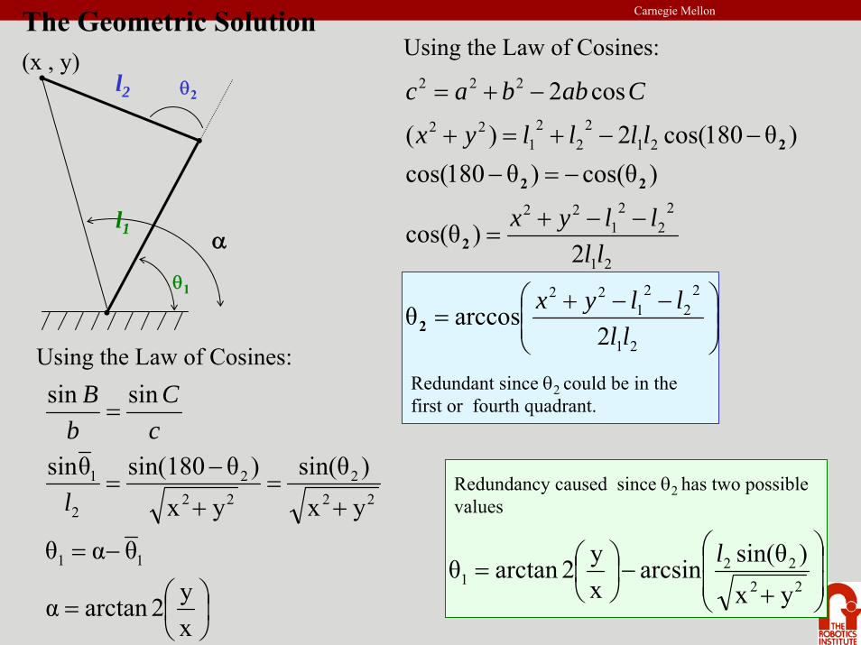
Carnegie MellonThe Geometric Solution

α

Using the Law of Cosines:

⎟⎟⎠

⎞⎜⎜⎝

⎛ −−+=

−−+=

−=−−−+=+

−+=

21

22

21

22

21

22

21

22

212

22

122

222

2arccosθ

2)cos(θ

)cos(θ)θ180cos()θ180cos(2)(

cos2

llllyx

llllyx

llllyx

Cabbac

2

2

22

2

Using the Law of Cosines:

⎟⎠⎞

⎜⎝⎛=

−=

+=

+

−=

=

xy2arctanα

θαθ

yx)sin(θ

yx)θsin(180θsin

sinsin

11

222

222

2

1

l

cC

bB

⎟⎟

⎠

⎞

⎜⎜

⎝

⎛

+−⎟⎠⎞

⎜⎝⎛=

2222

1yx

)sin(θarcsinxy2arctanθ l

Redundancy caused since θ2 has two possible values

Redundant since θ2 could be in the first or fourth quadrant.

l1

l2 θ2

θ1

(x , y)

Carnegie Mellon

( ) ( )( )

⎟⎟⎠

⎞⎜⎜⎝

⎛ −−+=∴

++=

+++=

+++++=

=+=+

++

++++

21

22

21

22

2

2212

22

1

211211212

22

1

211212

212

22

12

1211212

212

22

12

1

2222

2yxarccosθ

c2

)(sins)(cc2

)(sins2)(sins)(cc2)(cc

yx)2((1)

llll

llll

llll

llllllll

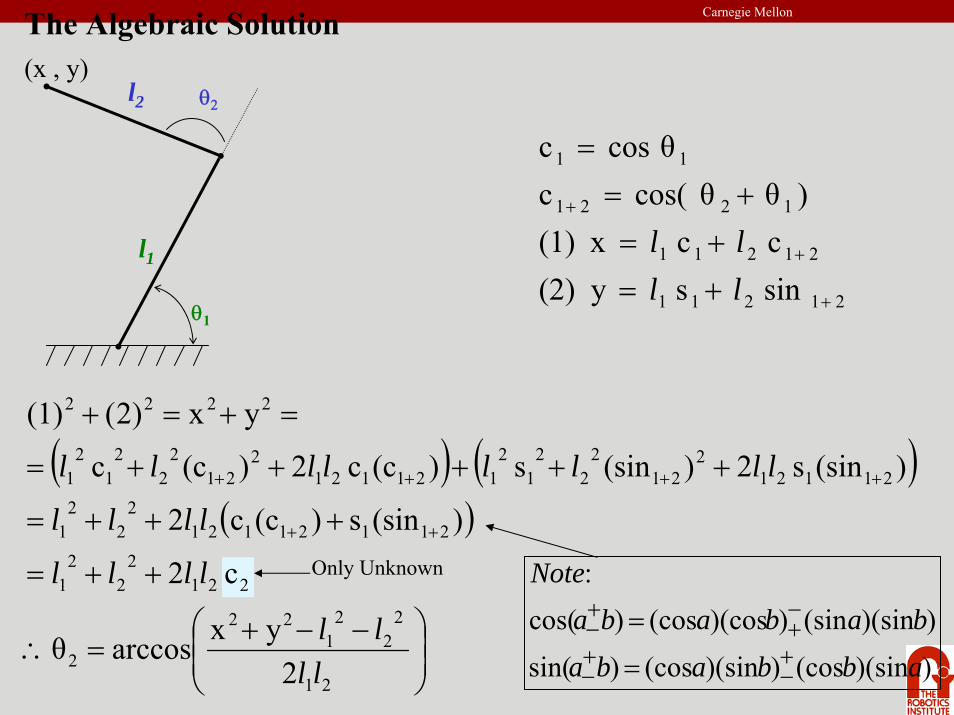
The Algebraic Solution

l1

l2 θ2

θ1

(x , y)

21211

21211

1221

11

sinsy(2)ccx(1)

)θcos( θccos θc

+

+

+

+=+=+=

=

llll

Only Unknown

))(sin(cos))(sin(cos)sin(

))(sin(sin))(cos(cos)cos(:

abbaba

bababaNote

+−

+−

−+

+−

=

=

Carnegie Mellon

))(sin(cos))(sin(cos)sin(

))(sin(sin))(cos(cos)cos(:

abbaba

bababaNote

+−

+−

−+

+−

=

=

)c(s)s(c cscss

sinsy

)()c(c ccc

ccx

2211221

12221211

21211

2212211

21221211

21211

llllll

ll

slsllsslll

ll

++=++=

+=

−+=−+=

+=

+

+

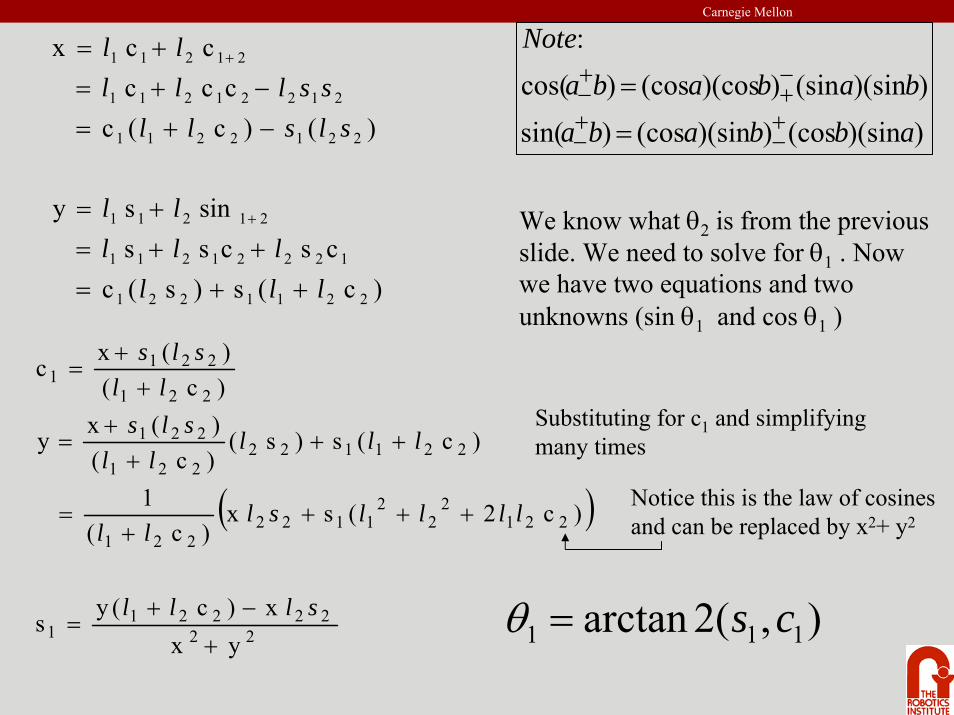
We know what θ2 is from the previous slide. We need to solve for θ1 . Now we have two equations and two unknowns (sin θ1 and cos θ1 )

( )

2222221

1

2212

22

1122221

221122221

221

221

2211

yxx)c(ys

)c2(sx)c(

1

)c(s)s()c()(xy

)c()(xc

+

−+=

++++

=

+++

+=

++

=

slll

llllslll

lllll

slsll

sls

Substituting for c1 and simplifying many times

Notice this is the law of cosines and can be replaced by x2+ y2

),(2arctan 111 cs=θ