An Introduction to Quantum Complexity Theory

Richard CleveUniversity of Calgary∗

Abstract

We give a basic overview of computational complexity, query com-plexity, and communication complexity, with quantum information in-corporated into each of these scenarios. The aim is to provide simplebut clear definitions, and to highlight the interplay between the threescenarios and currently-known quantum algorithms.

Complexity theory is concerned with the inherent cost required to solve in-formation processing problems, where the cost is measured in terms of variouswell-defined resources. In this context, a problem can usually be thought of asa function whose input is a problem instance and whose corresponding outputis the solution to it. Sometimes the solution is not unique, in which case theproblem can be thought of as a relation, rather than a function. Resources areusually measured in terms of: some designated elementary operations, mem-ory usage, or communication. We consider three specific complexity scenarios,which illustrate different advantages of working with quantum information:

1. Computational complexity

2. Query complexity

3. Communication complexity.

Despite the differences between these models, there are some intimate rela-tionships among them. The usefulness of many currently-known quantum al-gorithms is ultimately best expressed in the computational complexity model;however, virtually all of these algorithms evolved from algorithms in the querycomplexity model. The query complexity model is a natural setting for dis-covering interesting quantum algorithms, which frequently have interestingcounterparts in the computational complexity model. Quantum algorithmsin the query complexity model can also be transformed into protocols in the

∗Department of Computer Science, University of Calgary, Calgary, Alberta, Canada T2N1N4. Email: cleve@cpsc.ucalgary.ca.

1

communication complexity model that use quantum information (and some-times these are more efficient than any classical protocol can be). Also, thislatter relationship, taken in its contrapositive form, can be used to prove thatsome problems are inherently difficult in the query complexity model.

1 Computational complexity

In the computational complexity scenario, an input is encoded as a binarystring (say) and supplied to an algorithm, which must compute an outputstring corresponding to the input. For example, in the case of the factoringproblem, for input 100011 (representing 35 in binary), the valid outputs mightbe 000101 or 000111 (representing the factors of 35). The algorithm mustproduce the required output by a series of local operations. By this, we do notnecessarily mean “local in space”, but, rather, that each operation involves asmall portion of the data. In other words, a local operation is a transformationthat is confined to a small number of bits or qubits (such as two or three).The above property is satisfied by Turing machines and circuits, and also byquantum Turing machines [7, 21] and quantum circuits [22, 52] (see also [39]).We shall find it most convenient to work with circuit models here.

1.1 Classical circuits

For classical circuits, the basic operations can be taken as the binary ∧ (and)gate, the binary ∨ (or) gate, and the unary ¬ (not) gate. In Fig. 1 is aboolean circuit consisting of five gates that computes the parity of two bits.The inputs are denoted as x0 and x1, and the “data-flow” is from left to right.

¬

¬

∧

∧

∨

x0

x1HHHHHHHH

HHHH

Figure 1: A classical circuit for computing the parity of two bits.

The rightmost gate is designated as the output, whose value is x0 ⊕ x1, asrequired. This is the smallest circuit consisting of ∧, ∨, and ¬ gates thatcomputes the parity. Based on this fact, we could say that the computationalcomplexity of the binary parity function is five. But note that this value ishighly dependent on the specific set of basic operations that we started with.If we included the binary ⊕ (exclusive-or) gate as a basic operation then asingle gate suffices to compute the parity of two bits (Fig. 2).

2

x0

x1

HHHH

Figure 2: An alternative circuit for parity with one exclusive-or gate.

This illustrates a feature of the computational complexity model: the exactnumber of operations required to compute functions is quite sensitive to thetechnical choice of which basic operations to allow. The exact computationalcomplexity of simple problems involving a small number of bits is somewhatarbitrary.

Computational complexity is more meaningful when larger problems thatscale up are considered, such as the problem of computing the parity of n bits,x0, x1, . . . , xn−1. Using ⊕ gates, one can construct a tree with n−1 such gatesthat computes this parity. On the other hand, if only ∧, ∨, and ¬ gates areavailable then it appears that something like 5(n − 1) gates are needed. Inboth cases, the number of gates is O(n), and it is also straightforward to provethat a constant times n gates are necessary for both cases. A similar propertyholds for any computational complexity problem: changing from one set ofgates to any other set of gates (assuming that both sets are local and universal)can only affect computational complexity by a multiplicative constant. Thus,for any f : 0, 1∗ → 0, 1, its computational complexity is a well-definedfunction (of n, the length of the input to f) up to a multiplicative constant.

This is one reason why it is common to denote the computational com-plexity of functions using asymptotic notation that suppresses multiplicativeconstants. O(T (n)) means bounded above by c T (n) for some constant c > 0(for sufficiently large n). Also, Ω(T (n)) means bounded below by c T (n) forsome constant c > 0, and Θ(T (n)) means both O(T (n)) and Ω(T (n)). Acircuit is polynomially-bounded in size if its size is O(nd) for some constant d.

A matter that we have so far obscured concerns the treatment of the pa-rameter n (denoting the input size). Although each circuit is for some fixedvalue of n, we are also speaking of n as a freely varying parameter. For prob-lems where n is a variable (such as the problem of computing the parity ofn bits), an algorithm in the circuit model must actually be a circuit family(C1, C2, C3, . . .), where circuit Cn is responsible for all input instances of sizen. To be meaningful, a circuit family has to be uniform in that it can some-how be finitely specified. For example, for the aforementioned parity problem,a finite specification of a circuit family can be informally: “for input size n,Cn is a binary tree of ⊕-gates with x0, . . . , xn−1 at the leaves”. Formally, a

3

specification of a circuit family is an algorithm that maps each n to an explicitdescription of Cn. Technically, we ought to include the efficiency of the speci-fication algorithm as part of the computational cost of a circuit family. Thisraises the question of what formalism one uses to describe the specificationalgorithm. Note that if we try to use another circuit family for this then itrequires its own specification algorithm (and so on!), so this approach will notwork. There are sophisticated ways of dealing with uniformity; a very simpleway is to just use some non-circuit model, such as a Turing machine (runningin time, say, polynomial in n) for the circuit specification algorithm. At thispoint, the reader may wonder why one does not just use the Turing machinemodel to begin with. A big advantage of circuits is that their structural ele-ments are simple and easy to work with—and this appears to hold for quantumcircuits as well. Uniformity tends to be a straightforward technicality, thatcan be worked out after a circuit family is discovered; the discovery of thecircuit family is usually the interesting part of the algorithm design process.

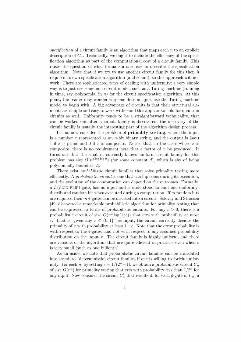
Let us now consider the problem of primality testing, where the inputis a number x represented as an n-bit binary string, and the output is (say)1 if x is prime and 0 if x is composite. Notice that, in the cases where x iscomposite, there is no requirement here that a factor of x be produced. Itturns out that the smallest currently-known uniform circuit family for thisproblem has size O(nd log log n) (for some constant d), which is shy of beingpolynomially-bounded [2].

There exist probabilistic circuit families that solve primality testing moreefficiently. A probabilistic circuit is one that can flip coins during its execution,and the evolution of the computation can depend on the outcomes. Formally,a /c (coin-flip) gate, has no input and is understood to emit one uniformly-distributed random bit when executed during a computation. If m random bitsare required then m /c-gates can be inserted into a circuit. Solovay and Strassen[49] discovered a remarkable probabilistic algorithm for primality testing thatcan be expressed in terms of probabilistic circuits. For any ε > 0, there is aprobabilistic circuit of size O(n3 log(1/ε)) that errs with probability at mostε. That is, given any x ∈ 0, 1n as input, the circuit correctly decides theprimality of x with probability at least 1−ε. Note that the error probability iswith respect to the /c-gates, and not with respect to any assumed probabilitydistribution on the input x. The circuit family is highly uniform, and thereare versions of the algorithm that are quite efficient in practice, even when εis very small (such as one billionth).

As an aside, we note that probabilistic circuit families can be translatedinto standard (deterministic) circuit families if one is willing to forfeit unifor-mity. For each n, by setting ε = 1/(2n+1), we obtain a probabilistic circuit Cn

of size O(n4) for primality testing that errs with probability less than 1/2n forany input. Now consider the circuit C ′

n that results if, for each /c-gate in Cn, a

4

uniformly distributed random bit is independently generated and substitutedfor that gate. This is a probabilistic construction that yields a deterministiccircuit C ′

n. For x ∈ 0, 1n, let px be the probability that the resulting C ′n

errs on input x. Then, for each x, px < 1/2n, so the probability that C ′n

errs for any x ∈ 0, 1n is strictly less than∑

x∈0,1n 1/2n = 1. Therefore,with probability greater than 0, C ′

n is correct for all of its 2n possible inputvalues. It follows that, for any n, a deterministic circuit of size O(n4) mustexist for primality testing. The problem is that there is no known efficient wayto explicitly construct the coin flips which yield a correct circuit. Thus, theimplied O(n4)-size circuit family for primality testing is merely established byan existence proof; this is an example of a non-uniform circuit family. The factthat uniform probabilistic circuit families can be converted into non-uniformdeterministic circuit families is theoretically noteworthy, but not practical.

A problem that is related to—but different from—primality testing is thefactoring problem, where the input is an n-bit number x, and the output isa list of the prime factors of x. This is apparently much harder than primalitytesting, since the smallest currently-known circuit family for this problem isprobabilistic and has size O(2

d√

n log n) (where d is a constant) [36, 41], which

is far from being polynomially-bounded. One of the reasons why quantumalgorithms are of interest is that there exists a quantum circuit family ofpolynomial-size that solves the factoring problem (this will be discussed later).

A problem that is closely related to the factoring problem is the order-finding problem, where the input is a pair of natural numbers a and Nthat are coprime (i.e. such that gcd(a,N) = 1), and the goal is to find thesmallest positive r such that ar mod N = 1 (there always exists such an r ∈1, . . . , N − 1). It turns out that a polynomial-size circuit family for theorder-finding problem can be converted into a polynomial-size probabilisticcircuit family for the factoring problem (and vice versa). In fact, the quantumcircuit for factoring is actually obtained via this relationship from a quantumcircuit that solves the order-finding problem.

Although we have represented circuits pictorially as data-flow diagrams,it is useful to be able to encode circuits as binary strings. There are severalreasonable encoding schemes. One such scheme encodes the graphical struc-ture of a circuit C as an m × m adjacency matrix (where m is the numberof gates plus the number of inputs in C), and then follows this by more bitsthat specify the labels of the nodes (e.g. ∧, ∨, ¬, x0, . . . , xn−1). Note that,using this encoding scheme, a circuit of size m has an encoding of O(m2)bits. There are more efficient encoding schemes, where the encodings are oflength O(m log m), and, for any “reasonable” encoding scheme, the length ofthe string that encodes C is polynomially-related to the size of C. Let e(C)denote a binary string that encodes the circuit C (relative to some reasonable

5

encoding scheme).A fundamental problem in classical computational complexity is the cir-

cuit satisfiability problem, which is defined as follows. Call a circuit satis-fiable if there exists an input string to the circuit for which the correspondingoutput value of the circuit is 1. For example, the circuit in Fig. 1 is satisfiable.The input to the circuit satisfiability problem is a binary string x = e(C) thatencodes some boolean circuit C, and the output is 1 if C is satisfiable, and0 otherwise. The best currently-known (deterministic or probabilistic) algo-rithm for circuit satisfiability is to simply try all possible inputs to C. Whene(C) encodes a circuit C with n inputs and m gates, this procedure takesO(2nmd) steps, where d is a constant that depends on the encoding schemeused (d = 2 suffices for most reasonable encoding schemes). In interestingcases, m is typically polynomial in n, so the dominant factor in this quantityis 2n. It is not known whether or not there is a polynomially-bounded cir-cuit family for circuit satisfiability. In fact, circuit satisfiability is one of theso-called NP -complete problems [19, 26], for which a polynomially-boundedcircuit family would yield polynomially-bounded circuits for all problems inNP .

1.2 Quantum circuits

To develop a theory of computational complexity for quantum information,it is natural to extend the notion of a circuit to a composition gates whichperform quantum operations on quantum bits (called qubits). The most generalquantum operations subsume all classical operations, which are frequently notreversible. It turns out that the quantum operations that seem to be the mostuseful in the context of quantum computation are those that are unitary (andhence reversible), as well as the von Neumann measurements.

Let us begin by recalling that the state of a system of m qubits can be de-scribed by associating an amplitide αx with each x ∈ 0, 1m (we restrict ourattention to pure quantum states). Each amplitude is a complex number andthere is a condition that

∑x∈0,1m |αx|2 = 1. Taken together, these ampli-

tudes constitute a point in a 2m-dimensional vector space. The computationalbasis associated with this vector space is |x〉 : x ∈ 0, 1m, and we follow theconvention of writing states as linear combinations of these basis elements:∑

x∈0,1m

αx |x〉 . (1)

Given a quantum state, it is impossible to access the values of the amplitudesdirectly. What one can do is perform a (von Neumann) measurement on eachqubit. If such an operation is performed then the result is a random m-bitstring y, distributed as Pr[y = x] = |αx|2, for each x ∈ 0, 1m. After this

6

measurement, the original quantum state is destroyed. One can also performa unitary operation on an m-qubit system, which is a linear transformation Ufor which UU † = I, where U † is the conjugate transpose of U . Such a unitarytransformation can be represented by a 2m × 2m matrix and will, in general,affect all of the m qubits.

For the purposes of quantum computation, we restrict the basic operationsto local unitary transformations that only involve a small number (say, oneor two) of the qubits. A one-qubit unitary operation can be described by2× 2 unitary matrix U . In the case where m = 1, this U transforms the stateα |0〉+ β |1〉 to the state α′ |0〉+ β′ |1〉, where(

α′

β′)

= U

(αβ

). (2)

In order to define the semantics of applying a one-qubit gate in the contextof an m-qubit system for m > 1, we introduce a tensor product operation.Suppose that an m-qubit system is in state

∑x∈0,1m αx |x〉 and an n-qubit

system is in state∑

y∈0,1n βy |y〉. Then the state of the combined system(consisting of m + n qubits) is defined to be the tensor product of the statesof the individual systems, which is ∑

x∈0,1m

αx |x〉 ∑

y∈0,1n

βy |y〉 =

∑x∈0,1m

y∈0,1n

αxβy |xy〉 . (3)

For example, ( 1√2|0〉− 1√

2|1〉)( 1√

2|0〉− 1√

2|1〉) = 1

2 |00〉− 12 |01〉− 1

2 |10〉+ 12 |11〉.

Now, applying a one-qubit U to the kth qubit of an m-qubit system is definedto be the unitary operation that maps each basis state

|x0 · · · xm−1〉 = |x0 · · · xk−2〉 |xk−1〉 |xk · · · xm−1〉to the state

|x0 · · · xk−2〉 (U |xk−1〉) |xk · · · xm−1〉(for each x ∈ 0, 1m). Note that, by linearity, this completely defines aunitary operation on an m-qubit system.

For example, the one-qubit Hadamard gate corresponds to the matrix

H = 1√2

(1 11 −1

), (4)

and, when it is applied to the second qubit of a two-qubit system, the resultingoperation is

1√2

1 1 0 01 −1 0 00 0 1 10 0 1 −1

(5)

7

(with respect to the ordering of basis states |00〉, |01〉, |10〉, |11〉). A quantumcircuit corresponding to such an operation is in Fig. 3, which denotes that thefirst (top) qubit is left unaltered and H is applied to the second qubit.

H

Figure 3: Quantum circuit applying a Hadamard gate to one of two qubits.

To construct nontrivial quantum circuits, it is necessary to include two-qubit unitary operations. A simple but quite useful two-qubit operation isthe controlled-not gate (c-not, for short), which, for all x, y ∈ 0, 1,transforms the basis state |x〉 |y〉 to the basis state |x〉 |y ⊕ x〉 (and this extendsto arbitrary quantum states by linearity). The notation for the c-not gatein quantum circuits is indicated in Fig. 4 (it is also known as the “reversibleexclusive-or” gate).

vm

Figure 4: Notation for the controlled-not (c-not) gate.

Note that the c-not gate corresponds to the unitary transformation1 0 0 00 1 0 00 0 0 10 0 1 0

. (6)

The semantics of the c-not gate extends to the context of m-qubit systemswith m > 2 in a manner similar to that of the one-qubit gates.

For basis states |x〉 |y〉, the effect of the c-not gate is essentially the sameas the classical two-bit gate that maps (x, y) to (x, x ⊕ y) (for all x, y ∈0, 1). This gate negates the second bit conditional on the first bit being1. For arbitrary quantum states, the behavior of this gate is more subtle.For example, although the classical gate never changes the value of its first“control” bit, the quantum gate sometimes does: applying the c-not gate to

8

state ( 1√2|0〉− 1√

2|1〉)( 1√

2|0〉− 1√

2|1〉) yields the state ( 1√

2|0〉+ 1√

2|1〉)( 1√

2|0〉−

1√2|1〉).A more general kind of two-qubit gate is the controlled-U gate, where

U is a 2 × 2 unitary matrix. This gate maps |0〉 |y〉 to |0〉 |y〉 and |1〉 |y〉 to|1〉 (U |y〉) (for all y ∈ 0, 1), and is denoted in Fig. 5.

vU

Figure 5: Notation for a controlled-U gate.

Note that the c-not gate is a special case of a controlled-U gate with

U =(

0 11 0

)(7)

(and this U itself is essentially a not gate).Now, suppose that we want to compute the and of two bits (i.e. take x0 and

x1 as input and produce x0 ∧x1 as output) using only the one- and two-qubitgates of the above form. This can be done in a manner that avoids irreversibleoperations via the quantum circuit in Fig. 6, where H is the Hadamard gate(Eq. 4) and

V =(

1 00 i

)(8)

(where i =√−1).

l lv vv v v

H V V † V H

≡ vv

lFigure 6: Quantum circuit simulating a c2-not (Toffoli) gate.

For any x0, x1, y ∈ 0, 1, setting the initial state of the qubits to |x0〉 |x1〉 |y〉and tracing through the execution of this circuit reveals that the final state

9

is |x0〉 |x1〉 |y ⊕ (x0 ∧ x1)〉. Thus, when y is initialized to 0, the final stateof the third qubit is |x0 ∧ x1〉 (and the explicit classical data, x0 ∧ x1, canbe extracted from this quantum state by a measurement). The three-qubitoperation that is simulated in Fig. 6 is a so-called Toffoli gate (also calleda controlled-controlled-not, or c2-not for short). See [3, 23, 47] forsome similar constructions.

For classical circuits, there are finite sets of gates which are universal in thesense that they can be used to simulate any other set of gates. For quantumcircuits, the situation is different, since the set of all unitary operations iscontinuous, and hence uncountable—even when restricted to one-qubit gates.If one starts with any finite set of quantum gates then the set of all unitaryoperations that can implemented is limited to some countable subset of all theunitary operations. In spite of this, there are meaningful ways to capture theimportant features associated with universal sets of gates.

First, it turns out that there are infinite sets consisting of one- and two-qubit of gates that are universal in the exact sense. For example, if the c-not gate as well as all unitary one-qubit gates are available then any k-qubitunitary operation can be simulated with O(4kk) such gates [3, 30]. Therefore,the overhead is constant when switching between different universal sets oflocal unitary gates (such as the set of all two-qubit gates and the set of allthree-qubit gates).

Moreover, there are finite sets of one- and two-qubit gates that are univer-sal in an approximate sense. The aforementioned one-qubit Hadamard gate H(Eq. 4) and the two-qubit controlled-V gate (where V is defined in Eq. 8)are an example of such a set. The precise result is best stated as a theorem.

Theorem 1 ([33, 48]) Let B be any two-qubit gate and ε > 0. Then thereexists a quantum circuit of size O(logd(1/ε)) (where d is a constant) consist-ing of only H and controlled-V gates which computes a unitary operationB′ that approximates B in the following sense. There exists a unit complexnumber λ (i.e. with |λ| = 1) such that ||B − λB′||2 ≤ ε.

In the above theorem, || · ||2 is the norm induced by Euclidean distance andλ is a “global phase factor”(which can be disregarded). Consequently, if B′

is substituted for B in some quantum circuit then the final state∑

x α′x |x〉

approximates the final state of the original circuit∑

x αx |x〉 in the sense that√∑x |λα′

x − αx|2 ≤ ε. This implies that if the final state is measured then theprobability of any event among the possible outcomes is affected by at most ε.The proof of Theorem 1 exploits the fact that the commutator of two unitaryoperators is not generally I (the identity operator), but it can converge veryquickly to I (see [33, 48] for details).

10

An example of another finite set of gates that is universal in the approxi-mate sense is: H, W , and c-not, where

W =(

1 00 eiπ/4

). (9)

In fact, with W and c-not gates, one can simulate a controlled-V gate,as shown in Fig. 7 (see also [9]).

l lv v

W

W

W †≡

vV

Figure 7: Simulation of a controlled-V gate (note: W † = W 7).

As in the classical case, the measure of computational complexity for quan-tum circuits is most interesting when large problems that scale up are consid-ered. Using sets of gates that are universal in the exact sense, computationalcomplexity can vary only by constant factors. On the other hand, using sets ofgates that are universal in the approximate sense, computational complexitycan vary by at most polylogarithmic factors: any circuit with m gates can besimulated within accuracy ε by a circuit in terms of a different set of basicoperations with O(m logd(m/ε)) gates. This is accomplished by simulatingeach of the m gates of the original circuit within accuracy ε/m, which resultsin a total accumulated error bounded by ε.

For example, consider the problem where the input is x0, x1, . . . , xn−1 andthe goal is to compute the conjunction x0 ∧ x1 ∧ · · · ∧ xn−1. In terms of H,W , and c-not gates, the computational complexity can be shown to be Θ(n),and, with another set of approximately uniform gates, the complexity may bedifferent, but it will remain between Ω(n) and O(n logd(n/ε)) (where d is someconstant and ε is the accuracy level required).

Since it seems inconceivable that it would ever be possible to physicallyimplement quantum gates with perfect accuracy, the need to ultimately workwith approximations of quantum gates is inevitable. Fortunately, due theunitarity of quantum operations, inaccuracies only scale up linearly with thenumber of gates involved in a circuit. And, if one employs quantum error-correcting codes and fault-tolerant techniques then even gates with constantinaccuracies (and that are subject to “decoherence”) can in principle be em-ployed in arbitrarily large quantum circuits [1, 31, 45] (see [42] for an extensivereview).

For quantum circuit families, we must also consider the issue of uniformity:a legitimate quantum circuit family should be finitely specifiable in a compu-

11

tationally efficient way. This can be defined as a straightforward extension ofthe uniformity definitions for classical circuit families, where the specificationalgorithm is classical and a finite set of gates that is approximately universal(such as H, W , and c-not) is used. All quantum algorithms proposed to datecan be expressed as circuit families that are uniform in this sense (see [39] forfurther comments).

Notwithstanding the above issues, a convenient practice is to allow perfectuniversal sets of gates, bearing in mind that: (a) they can always be approxi-mated using any finite set of gates that is approximately universal with onlya polylogarithmic penalty in the circuit size (even if the implementations ofthese gates are approximate); and (b) uniformity tends to be a straightforwardtechnicality (at least with the quantum algorithms discovered so far).

Perhaps the most remarkable quantum algorithm that has been discoveredto date is the factoring algorithm, due to Peter Shor [44].

Theorem 2 ([44]) There exists a quantum circuit family of size O(n2 logd(n/ε))that solves the factoring problem within accuracy ε (for some constant d).

Note that this circuit size is essentially exponentially smaller than the most effi-cient known classical probabilistic circuit for factoring (whose size is O(2

d√

n log n)).

The quantum factoring algorithm actually follows from an algorithm for theorder-finding problem, which in turn evolved from an algorithm in the querycomplexity model (explained in the next section).

The above result shows that, based on our current state of knowledge,quantum algorithms may be exponentially more efficient than classical algo-rithms for some problems. The next result shows that the gain in computa-tional efficiency cannot exceed one exponential.

Theorem 3 For any S(n)-qubit quantum circuit with T (n) gates there is aclassical probabilistic circuit with O(2S(n)T (n)3 log2(1/ε)) gates1 that simulatesit within accuracy ε in the following sense. After measuring the final state ofthe quantum circuit, the probability of any event among the outcomes differsfrom that of the classical circuit by at most ε.

The idea behind the proof of Theorem 3 is to store the values of all 2S(n) ampli-tudes associated with an S(n)-qubit quantum system in classical bits (to an ap-propriate level of precision). Then, for each of the T (n) gates, these amplitudesare updated to reflect the effect of the gate. At the end, the absolute value ofthe square of each amplitude is computed and the resulting probability distri-bution is sampled by using /c-gates. To obtain the upper bound in Theorem 3,it suffices to store each amplitude with T (n)+log(1/ε) bits of precision, which

1The T (n)3 log2(1/ε) factor can be replaced by a smaller but more complicated expression.

12

requires O(2S(n)(T (n)+log(1/ε))) bits in all. Since the effect of each quantumgate corresponds to multiplying the amplitude vector by a sparse 2S(n)×2S(n)

matrix, this entails O(2S(n)) arithmetic operations, which can be implementedby O(2S(n)(T (n) + log(1/ε))2) bit operations. Thus, the total number of clas-sical gates is O(2S(n)T (n)(T (n)+log(1/ε))2) ⊆ O(2S(n)T (n)3 log2(1/ε)). Also,the measurement process can be simulated with O(2S(n)T (n)2 log2(1/ε)) clas-sical gates.

A more refined argument than the one above can be used to show thatan S(n)-qubit circuit with T (n) gates can be simulated using space that ispolynomial in S(n) and T (n) (but still with an exponential number of oper-ations), and there are also more esoteric computational models that subsumethe power of quantum circuit families [25].

Regarding the circuit satisfiability problem, it is currently unknown whetheror not there exists a polynomially-bounded quantum circuit family that solvesit. What is known is that quantum algorithms can solve this problem quadrat-ically faster than the best currently-known classical algorithms for this prob-lem.

Theorem 4 There exists a quantum circuit family of size O(√

2n log(1/ε)md)that solves the circuit satisfiability problem within accuracy ε (for some con-stant d). Here, n and m measure the size of the input instance: n is thenumber of inputs to circuit C and m is the number of gates of C.

Note how this compares with the best currently-known classical circuitfamily for the circuit satisfiability problem, which has size O(2nmd). Bothquantities are exponential, but

√2n is nevertheless considerably smaller than

2n for large values of n. The quantum algorithm is a consequence of a re-markable algorithm in the query complexity model that was discovered byLov Grover [27] (explained in the next section).

2 Query complexity

This is an abstract scenario which can be thought of as a game, like “twentyquestions”. The goal is to determine some information by asking as few ques-tions as possible. This differs from the computational complexity scenario inthat the “input” is not presented as a binary string at the beginning of thecomputation. Rather, the input can be thought of as a “black box” comput-ing a function f : S → T , and the basic operations are queries, in which thealgorithm specifies a t from the domain of the function and receives the valuef(t) in response.

13

A natural example is that of “polynomial interpolation”, where f is anarbitrary polynomial of degree d

f(t) = c0 + c1t + · · ·+ cdtd (10)

and the goal is to determine the coefficients c0, c1, . . . , cd. It is well known thatd + 1 queries to f are necessary and sufficient to accomplish this.

In the classical case, an algorithm in this model can be represented by acircuit consisting of gates from some standard universal set (e.g. ∧, ∨, ¬) plusadditional gates to perform queries. For f : S → T , an f -query gate takest ∈ S as input and produces f(t) as output. In this scenario, since there are noinput bits related to the problem instance (the problem instance is embodiedin f), the inputs to the circuit are all set to constant values (such as 0).

In order to be able to adapt this model to settings involving quantuminformation, we slightly modify the form of the query gates so that theyare reversible. For example, for f : 0, 1n → 0, 1, define a reversible f -query gate as the mapping f : 0, 1n × 0, 1 → 0, 1n × 0, 1 such thatf(x, y) = (x, y⊕ f(x)) (for x ∈ 0, 1n and y ∈ 0, 1). Note that, for classicalalgorithms, reversible f -queries yield exactly the same information as the non-reversible kind. Any circuit that makes reversible f -queries can be convertedinto one that makes exactly the same number of non-reversible f -queries (andvice versa). Henceforth, all queries will be assumed to be in reversible form.

In the quantum case, an f -query is a unitary transformation that per-mutes the basis states according to the classical mapping determined by f (inreversible form). For example, for f : 0, 1n → 0, 1, an f -query gate is theunitary transformation that maps |x〉 |y〉 to |x〉 |y ⊕ f(x)〉 (for all x ∈ 0, 1n

and y ∈ 0, 1). One way of denoting f -queries in both classical and quantumcircuits is shown in Fig. 8 (for the case where f : 0, 12 → 0, 1).

m

f

Figure 8: Notation for an f -query gate when f : 0, 12 → 0, 1.

The first instance where a quantum algorithm was proven to outperformany classical algorithm was with Deutsch’s problem [21], where f : 0, 1 →0, 1 and f(t) = (c0 + c1t) mod 2, and the goal is to determine the value of

14

c1 (note that c1 = f(0) ⊕ f(1)). A classical circuit (in reversible form) thatcomputes c1 with two f -queries is shown in Fig. 9.

0

0

m mmf f

Figure 9: Classical circuit for Deutsch’s problem using two queries.

The inputs to the circuit are both initialized to 0, and the unary ⊕ operationbetween the two f -queries is a not gate. It is easy to see that the finalvalues of the two bits are 1 and c1. It can also be shown that no classicalalgorithm exists that computes c1 with a single f -query (since it is impossibleto determine f(0)⊕ f(1) from just f(0) or f(1) alone).

But the quantum circuit in Fig. 10 [18, 21] computes c1 with a singlef -query gate.

|0〉

|1〉 mf

H H

H H

Figure 10: Quantum circuit for Deutsch’s problem using one query.

Here the initial state of the two-qubit system is |0〉 |1〉 and its final state is(−1)c0 |c1〉 |1〉, which yields c1 when the first qubit is measured.

Query complexity can be pinned down more precisely than computationalcomplexity in that the “number of f -queries” is not sensitive to arbitrary tech-nical conventions. So, it makes sense to consider the exact query complexityof a problem independent of linear factors, and to say that the classical querycomplexity of Deutsch’s problem is two, whereas its quantum query complexityis one.

Although the above advantage is small, there are generalizations of Deutsch’sproblem for which the discrepancy between classical and quantum query com-plexity is much larger. One of these is Simon’s problem [46], which is definedas follows. For a function f : 0, 1n → 0, 1n, define s ∈ 0, 1n to be anXOR-mask of f if: f(x) = f(y) if and only if x ⊕ y ∈ 0n, s (where ⊕ isdefined over 0, 1n × 0, 1n bitwise). When s = 0n, f is a bijection, andwhen s 6= 0n, f is a two-to-one function with a special structure related to

15

s. In Simon’s problem, f : 0, 1n → 0, 1n is promised to have an XOR-mask s ∈ 0, 1n, and the goal is to find s by making queries to f . In thiscase, an f -query is the mapping (x, y) 7→ (x, y ⊕ f(x)) in the classical caseand |x〉 |y〉 7→ |x〉 |y ⊕ f(x)〉 in the quantum case (x, y ∈ 0, 1n). Note thatDeutsch’s problem is the special case of Simon’s problem where n = 1 (theXOR-mask is ¬c1 in this case).

It can be proven that any classical algorithm in the query model for Si-mon’s problem must make Ω(

√2n log(1/ε)) queries to f , even for probabilistic

circuits with query gates that are permitted to err with probability up to ε.On the other hand, there is a simple quantum circuit that solves this problemwith only O(n log(1/ε)) queries to f (see [46] for the details). There is also arefinement to Simon’s original algorithm that makes a polynomial number ofqueries and solves Simon’s problem exactly [11].

Although the primary resource under consideration is the number of queries,the number of auxiliary operations (i.e. the non-query gates) is also of interest,and it is desirable to bound both quantities. For Simon’s algorithm the totalnumber of gates is O(n2 log(1/ε)).

Simon’s problem demonstrates that, in the query complexity setting, thereare quantum algorithms that are exponentially more efficient than any classicalalgorithm. Although the query complexity scenario is somewhat abstract, thesignificance of algorithms in this model will become clear when we examinethe consequences of the order-finding problem in the query scenario,which is defined as follows. Let N be an n-bit integer and a ∈ 1, . . . , N − 1be a number such that gcd(a,N) = 1. In this version of the order-findingproblem, the function fa,N : 0, 1n ×0, 1n → 0, 1n ×0, 1n is defined as

fa,N (x, y) = (x, (axy) mod N). (11)

This is invertible if y is restricted to 0, . . . , N − 1 (and can be extendedto be invertible over its full domain by defining fa,N(x, y) = (x, y) for thecase where N ≤ y < 2n). The goal is to find the minimum r ∈ 1, . . . , N −1 such that ar mod N = 1 by making queries to fa,N (in this case, fa,N

is already in reversible form). Although there is no polynomially-boundedclassical circuit that solves this problem, Shor [44] discovered a quantum circuitthat solves it with probability 1−ε using only O(log(1/ε)) queries to fa,N andO(n2 logd(n/ε)) auxiliary gates (for some constant d). Detailed explanationsof the algorithm can be found in several sources, including [18, 32, 44].

A significant property of the function fa,N is that there exists a classi-cal circuit of size O(n2 log n log log n) that takes N (an n-bit number), a ∈1, . . . , N−1 (such that gcd(a,N) = 1), and x, y ∈ 0, 1n as input, and pro-duces fa,N (x, y) as output. In other words, given a and N , one can efficientlysimulate an fa,N -query gate. Moreover, this simulation can be implemented in

16

terms of quantum gates, such as not, c-not, and c2-not (using techniquesfor reversible classical computation [5]). By doing this simulation for eachfa,N -query gate in the quantum circuit for the order-finding problem, one ob-tains a quantum circuit of size O(n2 logd(n/ε)) that takes a and N as inputand produces the minimum positive r such that ar mod N = 1 as output withprobability 1 − ε. Thus, the algorithm in the query complexity model yieldsan algorithm in the computational complexity model for order-finding—andhence also for factoring. This is a specific instance of the following generalresult relating algorithms in the query complexity model to algorithms in thecomputational complexity model.

Theorem 5 Suppose that a function fz : 0, 1m → 0, 1k is associated witheach z ∈ 0, 1n (where m and k are functions of z), and that the classicalcomputational complexity of the function that maps (z, x) to fz(x) is boundedabove by R(n). Suppose also that there is a problem in the query complexitymodel where some property P (fz) is to be determined in terms of fz-queries,and that there is a quantum circuit that solves this problem using S(n) queriesto fz and T (n) auxiliary operations. Then the quantum computational com-plexity of the problem where the input is z ∈ 0, 1n and the output is the valueof the property P (fz) is O(R(n)S(n) + T (n)).

The circuit for the computational complexity problem is merely the circuitfor the query complexity problem with a circuit simulating each fz-query gatesubstituted for that fz-query gate.

A simple problem that seems natural in the query scenario is the searchproblem [27], where f : 0, 1n → 0, 1, and the goal is to find an x ∈ 0, 1n

such that f(x) = 1 (or to indicate that no such x exists). Any classicalalgorithm for this problem must make Ω(2n) f -queries, even if it is allowedto err with probability (say) 1

3 . Lov Grover [27] discovered a remarkablequantum algorithm that accomplishes this with O(

√2n) queries (some detailed

explanations of the algorithm are found in [8, 27, 37]). Grover’s result, withsome later refinements [8, 10, 14, 37, 54] incorporated into it, is summarizedas follows.

Theorem 6 ([27]) There is a quantum algorithm that solves the search prob-lem for f : 0, 1n → 0, 1 with O(

√2n log(1/ε)) queries to f , and errs with

probability at most ε.

The efficiency of the above algorithm has been shown to be optimal [6, 8,14, 53].

Clearly, Grover’s algorithm can also be used to solve the existentialsearch problem, where the goal is just to determine whether or not there

17

exists an x ∈ 0, 1n such that f(x) = 1 (a problem that also requires Ω(2n)queries in the classical case). Note the similarity between this existentialsearch problem and the circuit satisfiability problem. In fact, using Theo-rem 5, this algorithm in the query model translates into the algorithm forthe circuit satisfiability problem that is claimed in Theorem 4. The input ise(C), an encoding of a circuit C with m gates and n inputs that computes amapping C : 0, 1n → 0, 1, and the output should be 1 if there exists anx ∈ 0, 1n such that C(x) = 1, and 0 otherwise. The mapping that takes(e(C), x) to C(x) can be computed by a classical circuit with O(md) gates(where d is a constant that depends on the encoding scheme, and is usuallysmall). Also, the algorithm in Theorem 6 makes O(

√2n log(1/ε) n) auxiliary

operations. Therefore, applying Theorem 5, one obtains a quantum circuit ofsize O(

√2n log(1/ε) md) for the circuit satisfiability problem.

Let us now consider some variations and extensions of the existential searchproblem in the query model. We shall henceforth refer to the existential searchproblem as OR, defined as

OR(f) = (∃x)f(x), (12)

where f : 0, 1n → 0, 1 is accessed through f -queries. The name OR seemsnatural since

OR(f) = f(00 · · · 0) ∨ f(00 · · · 1) ∨ · · · ∨ f(11 · · · 1). (13)

Note that the complementary problem AND(f) = (∀x)f(x) has computationalcomplexity somewhat similar to that of OR, since (∀x)f(x) = ¬(∃x)¬f(x).

Some non-trivial extensions of OR and AND are the alternating quanti-fier problems, such as OR-AND , where there are two alternating quantifiers:

OR-AND(f) = (∃x1)(∀x2)f(x1, x2). (14)

Here, f : 0, 1n1 ×0, 1n2 → 0, 1, and n1, n2 are implicit parameters satis-fying n1+n2 = n. By a suitable recursive application of Grover’s algorithm forOR, this problem can be solved with O(

√2n n log(1/ε)) queries to f [13] (the

extra factor of√

n is to amplify the accuracy of the bottom level algorithmfor AND). In fact, one can extend the above to k alternations of quantifiers:

OR-AND- · · · -Q(f) = (∃x1)(∀x2) · · · (Qxk)f(x1, x2, . . . , xk), (15)

where Q ∈ OR,AND and Q ∈ ∃,∀, depending on whether k is even orodd, and f : 0, 1n1×· · ·×0, 1nk → 0, 1 with n1+· · ·nk = n. In this case,the recursive application of Grover’s technique makes O(

√2n nk−1 log(1/ε))

queries to f (see [13]; also [40] for a related result).

18

For all of these variations of OR and AND, it can be shown that anyclassical algorithm for one of these problems must make Ω(2n) queries, andthe quantum algorithms for these problems are all nearly quadratically moreefficient than this in the sense that they make O((2n)1/2+δ) queries, for anyδ > 0 and ε > 0. In fact, even if k, the number of alternations of ORand AND, is set to δn/2 log n (instead of being held constant), the quantumalgorithms make O((2n)1/2+δ) queries. All of these quantum algorithms alsohave counterparts for the corresponding problems in the computational model,where the function is specified by an encoding e(C) of a circuit C.

Another problem that has a similar flavor to these problems is the parityproblem (in the query scenario), defined as

PARITY (f) =

∑x∈0,1m

f(x)

mod 2. (16)

It can be shown that any classical algorithm requires Ω(2n) queries to solvePARITY , and it is natural to ask whether quantum algorithms can be quadrat-ically more efficient—or even O((2n)r), for some r < 1. One of the applicationsof the communication complexity model (explained in the next section) is toshow that this is not possible: at least Ω(2n/n) queries must be made by anyquantum algorithm. In fact, a stronger lower bound of 1

22n is also known[4, 24] (using different methods).

It is important to note that, although upper bounds in the query modeltranslate into upper bounds in the computational model, the converse of thisneed not be true. For example, it is conceivable that there is a polynomially-bounded circuit that solves the circuit parity problem, where the input ise(C), an encoding of a circuit C that computes a function f , and the outputis PARITY (f). Note how this latter problem is different from another versionof the parity problem in the computational scenario (discussed in Section 1.1),where the inputs are x0, x1, . . . , xn−1, and the goal is to compute x0 ⊕ x1 ⊕· · · ⊕ xn−1.

3 Communication complexity

In this model, there are two parties, traditionally referred to as Alice and Bob,who each receive an n-bit binary string as input (x = x0x1 . . . xn−1 for Aliceand y = y0y1 . . . yn−1 for Bob) and the goal is for them to determine the valueof some function of the of these 2n bits. The resource under consideration hereis the communication between the two parties, and an algorithm is a protocol,where the parties send information to each other (possibly in both directionsand over several rounds) until one of them (say, Bob) obtains the answer. This

19

model was introduced by Yao [51] and has been widely studied in the classicalcontext (see [35] for a survey).

An interesting example is the equality problem, where the function isEQ , defined as

EQ(x, y) =

1 if x = y0 if x 6= y.

A simple n-bit protocol for EQ is for Alice to just send her bits x0, . . . , xn−1

to Bob, after which Bob can evaluate the function by himself (in fact, thereis a similar n-bit protocol for any function). The interesting question iswhether or not the EQ function can be evaluated with fewer than n bitsof communication—after all, the goal here is only for Bob to acquire one bit.The answer depends on whether or not any error probability is permitted.

If Bob must acquire the value of EQ(x, y) with certainty then it turns outthat n bits of communication are necessary. Note that Alice sending the firstn− 1 bits of x will clearly not work, since the answer could critically dependon whether or not xn−1 = yn−1. The number of possible protocols to consideris quite large and an actual proof that n bits communication are necessary isnontrivial. The interested reader is referred to [35] for a proof.

On the other hand, for probabilistic protocols (where Alice and Bob canflip coins and base their behavior on the outcomes), if an error probability ofε > 0 is permitted then O(log(n) log(1/ε)) bits of communication are sufficient.As usual, we are not assuming anything about a probability distribution onthe input strings; the error probability is with respect to the random choicesmade by Alice and Bob, and it applies regardless of what x and y are.

We now describe an O(log(n) log(1/ε))-bit protocol for EQ. First of all,Alice and Bob agree on a finite field whose size is between 2n and 4n (sucha field always exists, and its elements can be represented as O(log(n))-bitstrings). Now, consider the two polynomials

px(t) = x0 + x1t + · · ·+ xn−1tn−1 (17)

py(t) = y0 + y1t + · · ·+ yn−1tn−1. (18)

For any value of t in the field, Alice can evaluate px(t) and Bob can evaluatepy(t). If x = y then the two polynomials are identical, so px(t) = py(t) forevery value of t. But, if x 6= y then, since px(t) and py(t) are polynomialsof degree n − 1, there can be at most n − 1 distinct values of t for whichpx(t) = py(t). Therefore, if a value of t is chosen randomly from the field thenthe probability that px(t) = py(t) is at most 1

2 . Now, the protocol proceeds asfollows. Alice chooses k = log(1/ε) independent random elements of the field,t1, . . . , tk, and then sends t1, . . . , tk and px(t1), . . . , px(tk) to Bob (this consistsof O(log(n) log(1/ε)) bits). Then Bob outputs 1 if and only if px(ti) = py(ti)

20

for all i ∈ 1, . . . , k. The probability that Bob erroneously outputs 1 whenx 6= y is at most 1/2k = ε.

Two other interesting communication complexity problems are the inter-section problem, where the function is IN , defined as

IN (x, y) = (x0 ∧ y0) ∨ (x1 ∧ y1) ∨ · · · ∨ (xn−1 ∧ yn−1) (19)

and the inner product problem, where the function is IP , defined as

IP(x, y) = (x0 ∧ y0)⊕ (x1 ∧ y1)⊕ · · · ⊕ (xn−1 ∧ yn−1). (20)

Intuitively, for IN, the inputs x and y can be thought as encodings of twosubsets of 0, . . . , n−1 and the output is a bit indicating whether or not theyintersect. Also, IP is the inner product of x and y as bit vectors in modulotwo arithmetic. The deterministic communication complexity of each of theseproblems is the same as that of EQ : any deterministic protocol requires nbits of communication. Also, it has been shown that both of these problemsare more difficult than EQ when probabilistic protocols are considered: anyprobabilistic protocol with error probability up to (say) 1

3 requires Ω(n) bitsof communication (see [15] for IP, and [29] for IN ; also [35]).

It is natural to ask whether any reduction in communication can be ob-tained by somehow using quantum information. Define a quantum commu-nication protocol as one where Alice and Bob can exchange messages thatconsist of qubits. In a more formal definition of this model, there is an a pri-ori system of m qubits, some of them in Alice’s possession and some of themin Bob’s possession. The initial state of all of these qubits can be assumed tobe |0〉, and Alice and Bob can each perform unitary transformations on thosequbits that are in their possession and they can also send qubits between them-selves (thereby changing the ownership of qubits). The output is then takenas the outcome of some measurement of Bob’s qubits. Various preliminaryresults about communication complexity with quantum information occurredin [12, 16, 20, 34, 52].

There are fundamental results in quantum information theory which implythat classical information cannot be “compressed” within quantum informa-tion [28]. For example, Alice cannot convey more than r classical bits ofinformation to Bob by sending him an r-qubit message. Based on this, onemight mistakenly think that there is no advantage to using quantum informa-tion in the communication complexity context. In fact, there exists a quantumcommunication protocol that solves IN whose qubit communication is approx-imately the square root of the bit communication of the best possible classicalprobabilistic protocol.

21

Theorem 7 ([13]) There exists a quantum protocol for the intersection prob-lem (IN) that uses O(

√n log(1/ε) log(n)) qubits of communication and errs

with probability at most ε.

Moreover, the quantum protocol can be adapted to actually find a point inthe intersection in the cases where IN (x, y) = 1. That is, to produce ani ∈ 0, . . . , n − 1 such that xi ∧ yi = 1. This problem, like IN, has classicalprobabilistic communication complexity Ω(n).

To understand the protocol in Theorem 7, it is helpful to think of the inputsx and y as functions rather than strings, and we introduce some notation thatmakes this explicit. For convenience, assume that n = 2k for some k (if notthen x and y can lengthened by padding them with zeroes), and define thefunctions fx, fy : 0, 1k → 0, 1 as

fx(i) = xi (21)fy(i) = yi (22)

where 0, 1k and 0, 1, . . . , 2k − 1 are identified in the natural way. Aliceand Bob’s input data can be thought of as fx and fy, rather than x and y(respectively). In particular, given x, Alice can simulate an fx-query that maps|i〉 |j〉 to |i〉 |j ⊕ fx(i)〉 (for all i ∈ 0, 1k and j ∈ 0, 1), and Bob can simulatefy-queries. (Although the resource that is of interest in this model is not thenumber of basic operations that Alice and Bob perform, it is worth noting that,Alice and Bob’s simulations of these queries can be explicitly implemented byreversible circuits with O(2kk) = O(n log(n)) basic operations).

To construct an efficient quantum protocol for IN, define the functionfx ∧ fy : 0, 1k → 0, 1 as (fx ∧ fy)(i) = fx(i) ∧ fy(i) (for i ∈ 0, 1k), andnote that IN (x, y) = OR(fx ∧ fy). Therefore, if Alice and Bob can somehowperform (fx ∧ fy)-queries then the value of IN (x, y) can be determined by

making O(√

2k log(1/ε)) = O(√

n log(1/ε)) such queries. The problem is thatneither Alice nor Bob individually have enough information to perform an(fx ∧ fy)-query (since this depends on both x and y). If Alice were to beginby sending x to Bob then Bob could make (fx ∧ fy)-queries on his own, butnote that this entails n bits of communication to begin with. Another, moreefficient, approach is for Alice and Bob to collectively simulate (fx ∧ fy)-queries by combining fx-queries (which Alice can perform) with fy-queries(which Bob can perform), and a small amount of communication. To see howthis is accomplished, consider the circuit in Fig. 11. First, ignoring the brokenvertical lines, note that the quantum circuit (composed of two fx-queries, twofy-queries, and one Toffoli gate) is equivalent to an (fx∧fy)-query. That is, itimplements the unitary transformation that maps the state |i〉 |0〉 |0〉 |j〉 to thestate |i〉 |0〉 |0〉 |j ⊕ (fx ∧ fy)(i)〉 (for all i ∈ 0, 1k , j ∈ 0, 1). This circuit

22

|0〉|0〉

fy fx fx fy

Bob Alice Bob

hh h

hhtt

≡

|0〉|0〉

fx∧fy

hFigure 11: Simulation of an (fx ∧ fy)-query in terms of fx-queries and fy-queries.

uses two extra qubits that are each initialized in state |0〉 and which incur nonet change.

Now, the protocol for IN can be thought of as Bob executing the algorithmin the query model for OR with the function fx ∧ fy, except that, wheneveran (fx ∧ fy)-query gate arises, he interacts with Alice to simulate the circuitin Fig. 11: first Bob performs an fy-query gate, then he sends the k +3 qubitsto Alice who performs some actions involving fx-queries and a Toffoli gate(shown between the two broken lines) and sends the qubits back to Bob, whoperforms another fy-query. Note that the total amount of communicationthat this entails is 2(k + 3) ∈ O(log n) qubits. Therefore, the total commu-nication for Bob’s simulation of the O(

√n log(1/ε)) queries to (fx ∧ fy) is

O(√

n log(1/ε) log(n)), as claimed in Theorem 7.More recently, Ran Raz has given an example of a communication com-

plexity problem which a quantum protocol can solve with exponentially lesscommunication than the best classical probabilistic protocol. The descriptionof the problem is more complicated than EQ, IN, and IP, and the reader isreferred to [43] for the details.

The methodology used to establish Theorem 7 involved the conversion ofan algorithm in the query model (for OR) to a communication protocol (forIN (x, y) = OR(fx ∧ fy)). This conversion can be stated in a more generalform.

Theorem 8 ([13]) Suppose that there is a quantum algorithm in the querymodel that computes P(f) in terms of T (k, ε) queries to f , where f : 0, 1k →

23

0, 1, and ε is a bound on the error probability. For n = 2k, define the com-munication problem P∧ : 0, 1n × 0, 1n → 0, 1 as P∧(x, y) = P (fx ∧ fy).Then there is a quantum protocol that solves P∧ with O(T (log(n), ε) log(n))qubits of communication. And a similar result holds for P∨(x, y) = P (fx ∨ fy)and P⊕(x, y) = P (fx ⊕ fy).

We conclude with a discussion of the quantum communication complexityof the inner product function IP. It has been shown [34] (see also [17]) that evenquantum protocols require communication Ω(n) for this problem, even whenthe error probability is permitted to be as large as (say) 1

3 . This fact, combinedwith Theorem 8 applied in its contrapositive form, can be used to establish alower bound for the parity problem in the query model (defined in Eq. 16).The main observation is that IP(x, y) = PARITY (fx∧fy). Suppose that thereis a quantum algorithm that computes PARITY (f) for f : 0, 1k → 0, 1by making T (k) f -queries (assume that the error probability is bounded by13). Then, by Theorem 8, there exists a quantum protocol that solves IPwith O(T (k)k) qubits of communication, where n = 2k is the size of theinput instance to IP. Since there is a lower bound of Ω(n) = Ω(2k) for thecommunication complexity of IP, we must have T (k)k ∈ Ω(2k), which impliesthat T (k) ∈ Ω(2k/k). This is an easy way to get a “ball park” lower boundfor the query complexity of PARITY, whose exact value is known to be 1

22k

by other methods [4, 24].

Acknowledgments

I would like to thank Michele Mosca for comments and help with the references.This research was partially supported by the Natural Sciences and EngineeringResearch Council of Canada.

References

[1] D. Aharonov and M. Ben-Or, “Fault-tolerant quantum computation withconstant error”, Proc. 29th Ann. ACM Symp. on Theory of Computing(STOC ’97), pp. 176–188, 1997.

[2] L. Adleman, C. Pomerance, R. Rumely, “On distinguishing prime numbersfrom composite numbers”, Annals of Mathematics, Vol. 117, pp. 173–206,1983.

[3] A. Barenco, C.H. Bennett, R. Cleve, D.P. DiVincenzo, N. Margolus,P. Shor, T. Sleator, J. Smolin, and H. Weinfurter, “Elementary gatesfor quantum computation”, Phys. Rev. A, Vol. 52, pp. 3457–3467, 1995.

24

[4] R. Beals, H. Buhrman, R. Cleve, M. Mosca, R. de Wolf, “Quantum lowerbounds by polynomials”, Proc. 39th Ann. IEEE Symp. on Foundations ofComputer Science (FOCS ’98), pp. 352–361, 1998.

[5] C.H. Bennett, “Logical reversibility of computation”, IBM J. of Researchand Development, Vol. 17, pp. 525–532, 1973.

[6] C.H. Bennett, E. Bernstein, G. Brassard, and U. Vazirani, “Strengthsand weaknesses of quantum computing”, SIAM J. on Computing, Vol. 26,No. 5, pp. 1510–1523, 1997.

[7] E. Bernstein and U.V. Vazirani, “Quantum complexity theory”, SIAM J.on Comput., Vol. 26, No. 5, pp. 1411–1473, 1997.

[8] M. Boyer, G. Brassard, P. Høyer, and A. Tapp, “Tight bounds on quantumsearching”, Fortschritte der Physik, Vol. 46, pp. 493–505, 1998. (An earlierversion appeared in Physcomp ’96.)

[9] P.O. Boykin, T. Mor, M. Pulver, V. Roychowdhury, and F. Vatan,“On universal and fault-tolerant quantum computing”, preprint quant-ph/9906054, 1999.

[10] G. Brassard, P. Høyer, and A. Tapp, “Quantum counting”, Proc. 25thICALP, Vol. 1443 of Lecture Notes in Computer Science, pp. 820–831(Springer), 1998.

[11] G. Brassard and P. Høyer, “An exact quantum polynomial-time algorithmfor Simon’s problem”, Proc. 5th Israeli Symp. on Theory of Computingand Systems (ISTCS ’97), pp. 12–23, 1997.

[12] H. Buhrman, R. Cleve, and W. van Dam, “Quantum entanglement andcommunication complexity”, preprint quant-ph/9705033, 1997.

[13] H. Buhrman, R. Cleve, and A. Wigderson, “Quantum vs. classical com-munication and computation”, Proc. 30th Ann. ACM Symp. on Theory ofComputing (STOC ’98), pp. 63-68, 1998.

[14] H. Buhrman, R. de Wolf, “Lower bounds for quantum search and deran-domization”, preprint quant-ph/9811046, 1998.

[15] B. Chor and O. Goldreich, “Unbiased bits from sources of weak random-ness and probabilistic communication complexity”, SIAM J. Comput.,Vol. 17, No. 2, pp. 230–261, 1988.

[16] R. Cleve and H. Buhrman, “Substituting quantum entanglement for com-munication”, Phys. Rev. A, Vol. 56, No. 2, pp. 1201–1204, 1997.

25

[17] R. Cleve, W. van Dam, M. Nielsen, and A. Tapp, “Quantum entangle-ment and the communication complexity of the inner product function”, toappear in Proc. 1st NASA Intl. Conf. on Quantum Computing and Quan-tum Communications, Vol. 1509 of Lecture Notes in Computer Science(Springer), 1998. preprint quant-ph/9708019, 1997.

[18] R. Cleve, A. Ekert, C. Macchiavello, and M. Mosca, “Quantum algorithmsrevisited”, Proc. of the Royal Society of London, Vol. A454, pp. 339–354,1998.

[19] S.A. Cook, “The complexity of theorem proving procedures”, Proc. 3rdAnn. ACM Symp. on Theory of Computing (STOC ’71), pp. 151–158,1971.

[20] W. van Dam, P. Høyer, A. Tapp, “Multiparty quantum communicationcomplexity”, preprint quant-ph/9710054, 1997.

[21] D. Deutsch, “Quantum theory, the Church-Turing principle and theuniversal quantum computer”, Proc. of the Royal Society of London,Vol. A400, pp. 96–117, 1985.

[22] D. Deutsch, “Quantum computational networks”, Proc. of the RoyalSociety of London, Vol. A425, pp. 73–90, 1989.

[23] D.P. DiVincenzo, “Quantum gates and circuits”, Proc. of the RoyalSociety of London, Vol. A454, pp. 261–276, 1998.

[24] E. Farhi, J. Goldstone, S. Gutmann, and M. Sipser, “A limit on the speedof quantum computation in determining parity.” Phys. Rev. Lett., Vol. 81,pp. 5442–5444, 1998.

[25] L. Fortnow and J. Rogers, “Complexity limitations on quantum computa-tion”, Proc. 13th IEEE Conf. on Computational Complexity, pp. 202–209,1998.

[26] M.R. Garey and D.S. Johnson, Computers and Intractibility: A Guide tothe Theory of NP-Completeness, W.H. Freeman, 1979.

[27] L.K. Grover, “A fast quantum mechanical algorithm for database search”,Proc. 28th Ann. ACM Symp. on Theory of Computing (STOC ’96),pp. 212–219, 1996.

[28] A.S. Holevo, “Some estimates of the information transmitted by quantumcommunication channels”, Problemy Peredachi Informatsii, Vol. 9, pp. 3–11, 1973. English translation in Problems of Information Transmission(USSR), Vol. 9, pp. 177–183, 1973.

26

[29] B. Kalyanasundaram and G. Schnitger, “The probabilistic communi-cation complexity of set intersection”, Proc. 2nd Conf. on Structure inComplexity Theory, pp. 41–49, 1987.

[30] E. Knill, personal communication, 1996.

[31] E. Knill, R. Laflamme, W. Zurek, “Threshold accuracy for quantumcomputation”, preprint quant-ph/9610011, 1996.

[32] A.Y. Kitaev, “Quantum measurements and the Abelian stabilizer prob-lem”, preprint quant-ph/9511026, 1995.

[33] A.Y. Kitaev, “Quantum computations: algorithms and error correction”,Russian Math. Surveys, Vol. 52, No. 6, pp. 1191-1249, 1997.

[34] I. Kremer, Quantum Communication, MSc Thesis, Computer ScienceDepartment, The Hebrew University, 1995.

[35] E. Kushilevitz and N. Nisan, Communication Complexity, (CambridgeUniversity Press), 1998.

[36] H. Lenstra and C. Pomerance, “A rigorous time bound for factoringintegers”, J. of the AMS, Vol. 5, No. 2, pp. 482–516, 1992.

[37] M. Mosca, “Quantum searching, counting and amplitude amplificationby eigenvector analysis”, MFCS ’98 workshop on Randomized Algorithms,1998.

[38] M. Mosca and A. Ekert, “The hidden subgroup problem and eigenvalueestimation on a quantum computer”, to appear in Proc. 1st NASA Intl.Conf. on Quantum Computing and Quantum Communications, Vol. 1509of Lecture Notes in Computer Science (Springer), 1998. preprint quant-ph/9903071, 1998.

[39] H. Nishimura and M. Ozawa, “Computational complexity of uniformquantum circuit families and quantum Turing machines”, preprint quant-ph/9906095, 1999.

[40] Y. Ozhigov, “Fast quantum verification for the formulas of predicatecalculus”, preprint quant-ph/9809015, 1998.

[41] C. Pomerance, “Fast rigorous factorization and discrete logarithm algo-rithms”, Discrete Algorithms and Complexity (Proc. Japan-US Joint Sem-inar on Discrete Algorithms and Complexity theory), pp. 119–143, 1987.

27

[42] J. Preskill, “Fault-tolerant quantum computation”, in Introduction toQuantum Computation and Information, edited by H.-K. Lo, S. Popescu,and T.P. Spiller (World Scientific), pp. 213–269, 1998.

[43] R. Raz, “Exponential separation of quantum and classical communicationcomplexity”, Proc. 31st Ann. ACM Symp. on Theory of Computing (STOC’99), pp. 358–367, 1999.

[44] P.W. Shor, “Polynomial-time algorithms for prime factorization and dis-crete logarithms on a quantum computer”, SIAM J. on Computing, Vol. 26,No. 5, pp. 1484–1509, 1997. (An earlier version appeared in FOCS ’94.)

[45] P.W. Shor, “Fault-tolerant quantum computation”, Proc. 37th Ann.IEEE Symp. on Foundations of Computer Science (FOCS ’96), pp. 56-65,1996.

[46] D. Simon, “On the power of quantum computation”, SIAM J. on Com-puting, Vol. 26, No. 5, pp. 1474–1483, 1997. (An earlier version appearedin FOCS ’94.)

[47] T. Sleator and H. Weinfurter, “Realizable universal quantum logic gates”,Phys. Rev. Lett., Vol. 74, pp. 4087–4090, 1995.

[48] R. Solovay, “Lie groups and quantum circuits”, paper in preparation,1999.

[49] R. Solovay and V. Strassen, “A fast Monte Carlo test for primality”,SIAM J. on Computing, Vol. 6, pp. 84–85, 1977. (Erratum in Vol. 7,p. 118, 1978.)

[50] U.V. Vazirani, “Strong communication complexity or generating quasi-random sequences from two communicating slightly-random sources”,Combinatorica, Vol. 7, No. 4, pp. 375–392, 1987.

[51] A. C.-C. Yao, “Some complexity questions related to distributive com-puting”, Proc. 11th Ann. ACM Symp. on Theory of Computing (STOC’79), pp. 209-213, 1979.

[52] A. C.-C. Yao, “Quantum circuit complexity”, Proc. 34th Ann. IEEESymp. on Foundations of Computer Science (FOCS ’93), pp. 352–361,1993.

[53] C. Zalka, “Grover’s quantum searching algorithm is optimal”, preprintquant-ph/9711070, 1997.

[54] C. Zalka, “A Grover-based quantum search of optimal order for an un-known number of marked elements”, preprint quant-ph/9902049, 1999.

28