An introduction to Psychometric Theory Theory of Data ... fileAn introduction to Psychometric Theory...

Model Fitting Coombs Objects Unfolding Scales Scaling Dispersion References

An introduction to Psychometric TheoryTheory of Data, Issues in Scaling

William Revelle

Department of PsychologyNorthwestern UniversityEvanston, Illinois USA

March, 2017

1 / 107


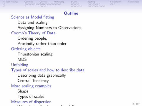
OutlineScience as Model fitting

Data and scalingAssigning Numbers to Observations

Coomb’s Theory of DataOrdering people,Proximity rather than order

Ordering objectsThurstonian scalingMDS

UnfoldingTypes of scales and how to describe data

Describing data graphicallyCentral Tendency

More scaling examplesShapeTypes of scales

Measures of dispersionWhat is the fundamental scale?

2 / 107


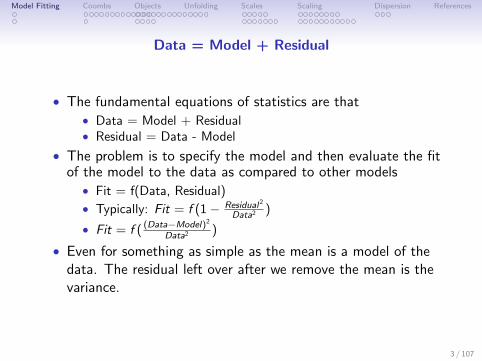
Data = Model + Residual

• The fundamental equations of statistics are that• Data = Model + Residual• Residual = Data - Model

• The problem is to specify the model and then evaluate the fitof the model to the data as compared to other models

• Fit = f(Data, Residual)

• Typically: Fit = f (1− Residual2

Data2 )

• Fit = f ( (Data−Model)2

Data2 )

• Even for something as simple as the mean is a model of thedata. The residual left over after we remove the mean is thevariance.

3 / 107


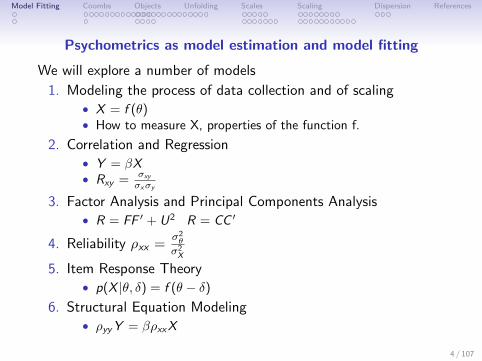
Psychometrics as model estimation and model fitting

We will explore a number of models

1. Modeling the process of data collection and of scaling• X = f (θ)• How to measure X, properties of the function f.

2. Correlation and Regression• Y = βX• Rxy =

σxy

σxσy

3. Factor Analysis and Principal Components Analysis• R = FF ′ + U2 R = CC ′

4. Reliability ρxx =σ2θ

σ2X

5. Item Response Theory• p(X |θ, δ) = f (θ − δ)

6. Structural Equation Modeling• ρyyY = βρxxX

4 / 107


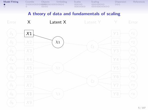
A theory of data and fundamentals of scaling

X

X 1

X 2

X 3

X 4

X 5

X 6

X 7

X 8

X 9

Error

δ1

δ2

δ3

δ4

δ5

δ6

δ7

δ8

δ9

χ1

χ2

χ3

ξ1

ξ2

Y

Y 1

Y 2

Y 3

Y 4

Y 5

Y 6

Y 7

Y 8

Error

ε1

ε2

ε3

ε4

ε5

ε6

ε7

ε8

Latent X Latent Y

5 / 107


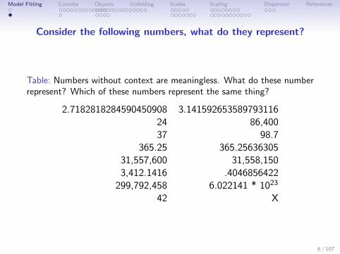
Consider the following numbers, what do they represent?

Table: Numbers without context are meaningless. What do these numberrepresent? Which of these numbers represent the same thing?

2.7182818284590450908 3.14159265358979311624 86,40037 98.7

365.25 365.2563630531,557,600 31,558,1503,412.1416 .4046856422

299,792,458 6.022141 * 1023

42 X

6 / 107


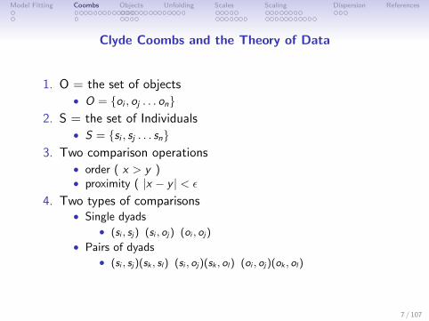
Clyde Coombs and the Theory of Data

1. O = the set of objects• O = {oi , oj . . . on}

2. S = the set of Individuals• S = {si , sj . . . sn}

3. Two comparison operations• order ( x > y )• proximity ( |x − y | < ε

4. Two types of comparisons• Single dyads

• (si , sj) (si , oj) (oi , oj)

• Pairs of dyads• (si , sj)(sk , sl) (si , oj)(sk , ol) (oi , oj)(ok , ol)

7 / 107


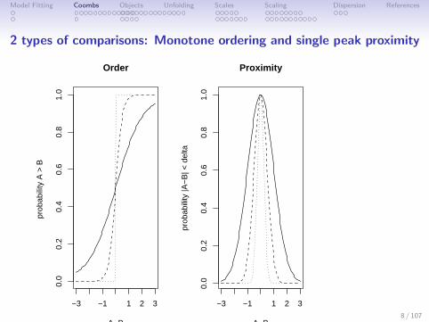
2 types of comparisons: Monotone ordering and single peak proximity

−3 −1 1 2 3

0.0

0.2

0.4

0.6

0.8

1.0

Order

A−B

prob

abili

ty A

> B

−3 −1 1 2 3

0.0

0.2

0.4

0.6

0.8

1.0

Proximity

A−B

prob

abili

ty |A

−B

| < d

elta

8 / 107


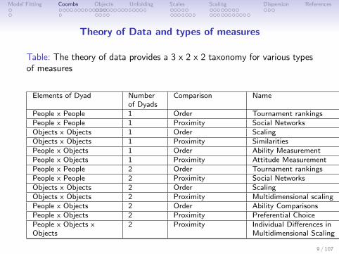
Theory of Data and types of measures

Table: The theory of data provides a 3 x 2 x 2 taxonomy for various typesof measures

Elements of Dyad Numberof Dyads

Comparison Name Chapter

People x People 1 Order Tournament rankings Theory of Data ??People x People 1 Proximity Social Networks Theory of Data ??Objects x Objects 1 Order Scaling Thurstonian scaling ??Objects x Objects 1 Proximity Similarities Multidimensional scaling ??People x Objects 1 Order Ability Measurement Test Theory ??, ??People x Objects 1 Proximity Attitude Measurement Attitudes ??People x People 2 Order Tournament rankingsPeople x People 2 Proximity Social Networks Theory of Data ??Objects x Objects 2 Order Scaling Theory of Data ??Objects x Objects 2 Proximity Multidimensional scaling Theory of Data ??People x Objects 2 Order Ability ComparisonsPeople x Objects 2 Proximity Preferential Choice Unfolding Theory ??People x Objects x 2 Proximity Individual Differences inObjects Multidimensional Scaling

9 / 107


Tournaments to order people (or teams)

1. Goal is to order the players by outcome to predict futureoutcomes

2. Complete Round Robin comparisons• Everyone plays everyone• Requires N ∗ (N − 1)/2 matches• How do you scale the results?

3. Partial Tournaments – Seeding and group play• World Cup• NCAA basketball• Is the winner really the best?• Can you predict other matches

10 / 107


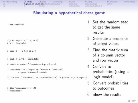
Simulating a hypothetical chess game

> set.seed(42)

> p <- seq(-1.5, 1.5, 0.2)

> n <- length(p)

> pdif <- -p %+% t( p )

> prob <- 1/(1 + exp(pdif))

> match <- matrix(rbinom(n*n,1,prob),n,n)

> tournament <- t(upper.tri(match) * (1-match))

+ upper.tri(match)*match

> colnames (tournament) <- rownames(match) <- paste("P",1:n,sep="")

> diag(tournament) <- NA

> tournament

1. Set the random seedto get the sameresults

2. Generate a sequenceof latent values

3. Find the matrix sumof a column vectorand row vector

4. Convert toprobabilities (using alogit model)

5. Convert probabilitiesto outcomes

6. Show the results

11 / 107


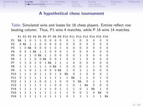
A hypothetical chess tournament

Table: Simulated wins and losses for 16 chess players. Entries reflect rowbeating column. Thus, P1 wins 4 matches, while P 16 wins 14 matches.

P1 P2 P3 P4 P5 P6 P7 P8 P9 P10 P11 P12 P13 P14 P15 P16

P1 NA 1 0 1 1 0 0 0 0 0 1 0 0 0 0 0

P2 0 NA 1 1 0 0 0 0 0 0 0 0 0 0 0 0

P3 1 0 NA 0 0 0 1 0 1 0 0 0 0 0 0 0

P4 0 0 1 NA 1 1 0 0 0 1 0 0 0 0 0 0

P5 0 1 1 0 NA 1 1 0 0 0 0 1 0 0 0 0

P6 1 1 1 0 0 NA 0 0 1 0 0 1 0 0 0 0

P7 1 1 0 1 0 1 NA 1 1 1 0 0 0 0 0 0

P8 1 1 1 1 1 1 0 NA 1 0 0 0 1 1 0 0

P9 1 1 0 1 1 0 0 0 NA 1 0 1 1 0 0 0

P10 1 1 1 0 1 1 0 1 0 NA 0 1 0 0 0 1

P11 0 1 1 1 1 1 1 1 1 1 NA 1 1 0 1 0

P12 1 1 1 1 0 0 1 1 0 0 0 NA 0 1 1 0

P13 1 1 1 1 1 1 1 0 0 1 0 1 NA 0 0 0

P14 1 1 1 1 1 1 1 0 1 1 1 0 1 NA 1 0

P15 1 1 1 1 1 1 1 1 1 1 0 0 1 0 NA 0

P16 1 1 1 1 1 1 1 1 1 0 1 1 1 1 1 NA

12 / 107


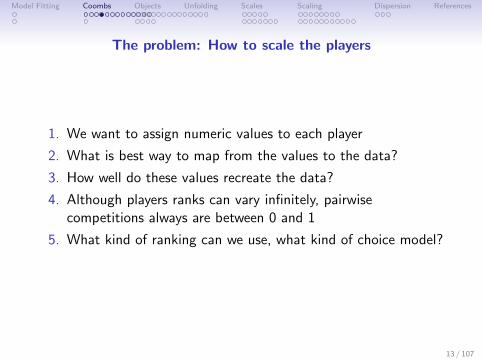
The problem: How to scale the players

1. We want to assign numeric values to each player

2. What is best way to map from the values to the data?

3. How well do these values recreate the data?

4. Although players ranks can vary infinitely, pairwisecompetitions always are between 0 and 1

5. What kind of ranking can we use, what kind of choice model?

13 / 107


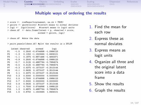
Multiple ways of ordering the results

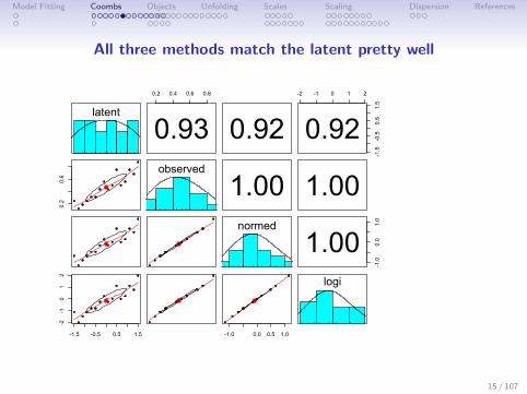
> score <- rowMeans(tournament, na.rm = TRUE)

> qscore <- qnorm(score) #convert means to normal deviates

> logi <- logit(score) #convert means to logit units

> chess.df <- data.frame(latent = p, observed = score,

normed = qscore, logi)

> chess.df #show the data

> pairs.panels(chess.df) #plot the results in a SPLOM

latent observed normed logi

P1 -1.5 0.2500 -0.6744898 -1.0986123

P2 -1.3 0.1250 -1.1503494 -1.9459101

P3 -1.1 0.1875 -0.8871466 -1.4663371

P4 -0.9 0.2500 -0.6744898 -1.0986123

P5 -0.7 0.3125 -0.4887764 -0.7884574

P6 -0.5 0.3125 -0.4887764 -0.7884574

P7 -0.3 0.4375 -0.1573107 -0.2513144

P8 -0.1 0.5625 0.1573107 0.2513144

P9 0.1 0.4375 -0.1573107 -0.2513144

P10 0.3 0.5000 0.0000000 0.0000000

P11 0.5 0.7500 0.6744898 1.0986123

P12 0.7 0.5000 0.0000000 0.0000000

P13 0.9 0.5625 0.1573107 0.2513144

P14 1.1 0.7500 0.6744898 1.0986123

P15 1.3 0.6875 0.4887764 0.7884574

P16 1.5 0.8750 1.1503494 1.9459101

1. Find the mean foreach row

2. Express these asnormal deviates

3. Express means aslogit units

4. Organize all three andthe original latentscore into a dataframe

5. Show the results

6. Graph the results

14 / 107


All three methods match the latent pretty well

latent

0.2 0.4 0.6 0.8

0.93 0.92-2 -1 0 1 2

-1.5

-0.5

0.5

1.5

0.92

0.2

0.6

observed

1.00 1.00normed

-1.0

0.0

1.0

1.00

-1.5 -0.5 0.5 1.5

-2-1

01

2

-1.0 0.0 0.5 1.0

logi

15 / 107


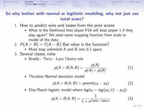
So why bother with normal or logitistic modeling, why not just usetotal score?

1. How to predict wins and losses from the prior scores• What is the likelihood that player P16 will beat player 1 if they

play again? We need some mapping function from scale tomodel of the data

2. P(A > B) = f (A− B) But what is the function?• Must map unlimited A and B into 0-1 space

3. Several classic rules• Bradly - Terry - Luce Choice rule

p(A > B|A,B) =p(A)

p(A) + p(B). (1)

• Thurston Normal deviation model

p(A > B|A,B) = pnorm(zA − zB) (2)

• Elos/Rasch logistic model where logitA = log(pA/(1− pA))

p(A > B|A,B) =1

1 + e(logitB−logitA)(3)

16 / 107


How well do these various models fit the data?

1. Generate the model of wins and losses• Compare to the data• Find the residuals• Summarize these results

2. Can do it “by hand”• Take the scale model, model the data• Find residuals• Find a goodness of fit

3. Can use a psych function: scaling.fits to find the fit• Although we don’t need to know how the function works, it is

possible to find out by using just the function name• To find out how to call a function, ?function, e.g., ?scaling.fits• To run a function, just say function() e.g. scaling.fits(model,

data)

17 / 107


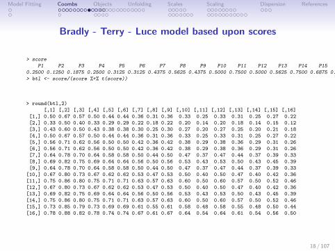
Bradly - Terry - Luce model based upon scores

> score


0.2500 0.1250 0.1875 0.2500 0.3125 0.3125 0.4375 0.5625 0.4375 0.5000 0.7500 0.5000 0.5625 0.7500 0.6875 0.8750

> btl <- score/(score %+% t(score))

> round(btl,2)

[,1] [,2] [,3] [,4] [,5] [,6] [,7] [,8] [,9] [,10] [,11] [,12] [,13] [,14] [,15] [,16]

[1,] 0.50 0.67 0.57 0.50 0.44 0.44 0.36 0.31 0.36 0.33 0.25 0.33 0.31 0.25 0.27 0.22

[2,] 0.33 0.50 0.40 0.33 0.29 0.29 0.22 0.18 0.22 0.20 0.14 0.20 0.18 0.14 0.15 0.12

[3,] 0.43 0.60 0.50 0.43 0.38 0.38 0.30 0.25 0.30 0.27 0.20 0.27 0.25 0.20 0.21 0.18

[4,] 0.50 0.67 0.57 0.50 0.44 0.44 0.36 0.31 0.36 0.33 0.25 0.33 0.31 0.25 0.27 0.22

[5,] 0.56 0.71 0.62 0.56 0.50 0.50 0.42 0.36 0.42 0.38 0.29 0.38 0.36 0.29 0.31 0.26

[6,] 0.56 0.71 0.62 0.56 0.50 0.50 0.42 0.36 0.42 0.38 0.29 0.38 0.36 0.29 0.31 0.26

[7,] 0.64 0.78 0.70 0.64 0.58 0.58 0.50 0.44 0.50 0.47 0.37 0.47 0.44 0.37 0.39 0.33

[8,] 0.69 0.82 0.75 0.69 0.64 0.64 0.56 0.50 0.56 0.53 0.43 0.53 0.50 0.43 0.45 0.39

[9,] 0.64 0.78 0.70 0.64 0.58 0.58 0.50 0.44 0.50 0.47 0.37 0.47 0.44 0.37 0.39 0.33

[10,] 0.67 0.80 0.73 0.67 0.62 0.62 0.53 0.47 0.53 0.50 0.40 0.50 0.47 0.40 0.42 0.36

[11,] 0.75 0.86 0.80 0.75 0.71 0.71 0.63 0.57 0.63 0.60 0.50 0.60 0.57 0.50 0.52 0.46

[12,] 0.67 0.80 0.73 0.67 0.62 0.62 0.53 0.47 0.53 0.50 0.40 0.50 0.47 0.40 0.42 0.36

[13,] 0.69 0.82 0.75 0.69 0.64 0.64 0.56 0.50 0.56 0.53 0.43 0.53 0.50 0.43 0.45 0.39

[14,] 0.75 0.86 0.80 0.75 0.71 0.71 0.63 0.57 0.63 0.60 0.50 0.60 0.57 0.50 0.52 0.46

[15,] 0.73 0.85 0.79 0.73 0.69 0.69 0.61 0.55 0.61 0.58 0.48 0.58 0.55 0.48 0.50 0.44

[16,] 0.78 0.88 0.82 0.78 0.74 0.74 0.67 0.61 0.67 0.64 0.54 0.64 0.61 0.54 0.56 0.50

18 / 107


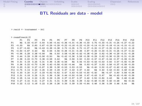
BTL Residuals are data - model

> resid <- tournament - btl

> round(resid,2)


P1 NA 0.33 -0.57 0.50 0.56 -0.44 -0.36 -0.31 -0.36 -0.33 0.75 -0.33 -0.31 -0.25 -0.27 -0.22

P2 -0.33 NA 0.60 0.67 -0.29 -0.29 -0.22 -0.18 -0.22 -0.20 -0.14 -0.20 -0.18 -0.14 -0.15 -0.12

P3 0.57 -0.60 NA -0.43 -0.38 -0.38 0.70 -0.25 0.70 -0.27 -0.20 -0.27 -0.25 -0.20 -0.21 -0.18

P4 -0.50 -0.67 0.43 NA 0.56 0.56 -0.36 -0.31 -0.36 0.67 -0.25 -0.33 -0.31 -0.25 -0.27 -0.22

P5 -0.56 0.29 0.38 -0.56 NA 0.50 0.58 -0.36 -0.42 -0.38 -0.29 0.62 -0.36 -0.29 -0.31 -0.26

P6 0.44 0.29 0.38 -0.56 -0.50 NA -0.42 -0.36 0.58 -0.38 -0.29 0.62 -0.36 -0.29 -0.31 -0.26

P7 0.36 0.22 -0.70 0.36 -0.58 0.42 NA 0.56 0.50 0.53 -0.37 -0.47 -0.44 -0.37 -0.39 -0.33

P8 0.31 0.18 0.25 0.31 0.36 0.36 -0.56 NA 0.44 -0.53 -0.43 -0.53 0.50 0.57 -0.45 -0.39

P9 0.36 0.22 -0.70 0.36 0.42 -0.58 -0.50 -0.44 NA 0.53 -0.37 0.53 0.56 -0.37 -0.39 -0.33

P10 0.33 0.20 0.27 -0.67 0.38 0.38 -0.53 0.53 -0.53 NA -0.40 0.50 -0.47 -0.40 -0.42 0.64

P11 -0.75 0.14 0.20 0.25 0.29 0.29 0.37 0.43 0.37 0.40 NA 0.40 0.43 -0.50 0.48 -0.46

P12 0.33 0.20 0.27 0.33 -0.62 -0.62 0.47 0.53 -0.53 -0.50 -0.40 NA -0.47 0.60 0.58 -0.36

P13 0.31 0.18 0.25 0.31 0.36 0.36 0.44 -0.50 -0.56 0.47 -0.43 0.47 NA -0.43 -0.45 -0.39

P14 0.25 0.14 0.20 0.25 0.29 0.29 0.37 -0.57 0.37 0.40 0.50 -0.60 0.43 NA 0.48 -0.46

P15 0.27 0.15 0.21 0.27 0.31 0.31 0.39 0.45 0.39 0.42 -0.48 -0.58 0.45 -0.48 NA -0.44

P16 0.22 0.12 0.18 0.22 0.26 0.26 0.33 0.39 0.33 -0.64 0.46 0.36 0.39 0.46 0.44 NA

19 / 107


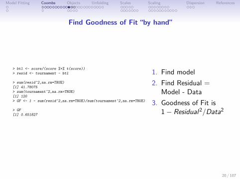
Find Goodness of Fit “by hand”

> btl <- score/(score %+% t(score))

> resid <- tournament - btl

> sum(resid^2,na.rm=TRUE)

[1] 41.78075

> sum(tournament^2,na.rm=TRUE)

[1] 120

> GF <- 1 - sum(resid^2,na.rm=TRUE)/sum(tournament^2,na.rm=TRUE)

> GF

[1] 0.651827

1. Find model

2. Find Residual =Model - Data

3. Goodness of Fit is1− Residual2/Data2

20 / 107


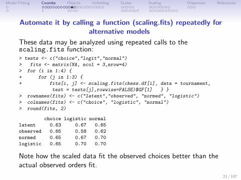
Automate it by calling a function (scaling.fits) repeatedly foralternative models

These data may be analyzed using repeated calls to thescaling.fits function:> tests <- c("choice","logit","normal")

> fits <- matrix(NA, ncol = 3,nrow=4)

> for (i in 1:4) {

+ for (j in 1:3) {

+ fits[i, j] <- scaling.fits(chess.df[i], data = tournament,

test = tests[j],rowwise=FALSE)$GF[1] } }

> rownames(fits) <- c("latent","observed", "normed", "logistic")

> colnames(fits) <- c("choice", "logistic", "normal")

> round(fits, 2)

choice logistic normal

latent 0.63 0.67 0.65

observed 0.65 0.58 0.62

normed 0.65 0.67 0.70

logistic 0.65 0.70 0.70

Note how the scaled data fit the observed choices better than theactual observed orders fit.

21 / 107


Advanced: The scaling.fits function> scaling.fits <-

function (model, data, test = "logit", digits = 2, rowwise = TRUE) {

model <- as.matrix(model)

data <- as.matrix(data)

if (test == "choice") {

model <- as.vector(model)

if (min(model) <= 0)

model <- model - min(model)

prob = model/(model %+% t(model))

}

else {

pdif <- model %+% -t(model)

if (test == "logit") {

prob <- 1/(1 + exp(-pdif))

}

else {

if (test == "normal") {

prob <- pnorm(pdif)

}

}

}

if (rowwise) {

prob = 1 - prob

}

error <- data - prob

sum.error2 <- sum(error^2, na.rm = TRUE)

sum.data2 <- sum(data^2, na.rm = TRUE)

gof <- 1 - sum.error2/sum.data2

fit <- list(GF = gof, original = sum.data2, resid = sum.error2,

residual = round(error, digits))

return(fit)

}22 / 107


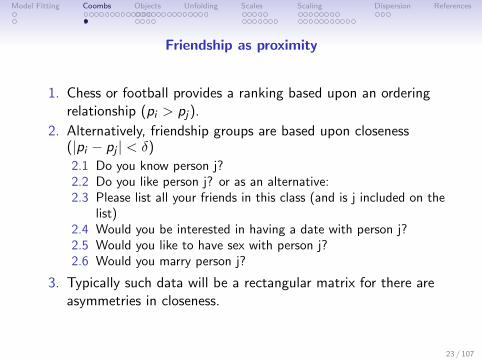
Friendship as proximity

1. Chess or football provides a ranking based upon an orderingrelationship (pi > pj).

2. Alternatively, friendship groups are based upon closeness(|pi − pj | < δ)

2.1 Do you know person j?2.2 Do you like person j? or as an alternative:2.3 Please list all your friends in this class (and is j included on the

list)2.4 Would you be interested in having a date with person j?2.5 Would you like to have sex with person j?2.6 Would you marry person j?

3. Typically such data will be a rectangular matrix for there areasymmetries in closeness.

23 / 107


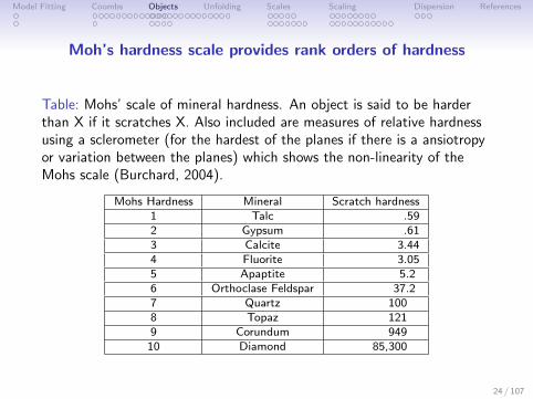
Moh’s hardness scale provides rank orders of hardness

Table: Mohs’ scale of mineral hardness. An object is said to be harderthan X if it scratches X. Also included are measures of relative hardnessusing a sclerometer (for the hardest of the planes if there is a ansiotropyor variation between the planes) which shows the non-linearity of theMohs scale (Burchard, 2004).

Mohs Hardness Mineral Scratch hardness1 Talc .592 Gypsum .613 Calcite 3.444 Fluorite 3.055 Apaptite 5.26 Orthoclase Feldspar 37.27 Quartz 1008 Topaz 1219 Corundum 949

10 Diamond 85,300

24 / 107


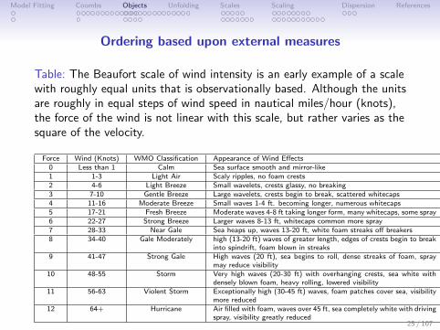
Ordering based upon external measures

Table: The Beaufort scale of wind intensity is an early example of a scalewith roughly equal units that is observationally based. Although the unitsare roughly in equal steps of wind speed in nautical miles/hour (knots),the force of the wind is not linear with this scale, but rather varies as thesquare of the velocity.

Force Wind (Knots) WMO Classification Appearance of Wind Effects0 Less than 1 Calm Sea surface smooth and mirror-like1 1-3 Light Air Scaly ripples, no foam crests2 4-6 Light Breeze Small wavelets, crests glassy, no breaking3 7-10 Gentle Breeze Large wavelets, crests begin to break, scattered whitecaps4 11-16 Moderate Breeze Small waves 1-4 ft. becoming longer, numerous whitecaps5 17-21 Fresh Breeze Moderate waves 4-8 ft taking longer form, many whitecaps, some spray6 22-27 Strong Breeze Larger waves 8-13 ft, whitecaps common more spray7 28-33 Near Gale Sea heaps up, waves 13-20 ft, white foam streaks off breakers8 34-40 Gale Moderately high (13-20 ft) waves of greater length, edges of crests begin to break

into spindrift, foam blown in streaks9 41-47 Strong Gale High waves (20 ft), sea begins to roll, dense streaks of foam, spray

may reduce visibility10 48-55 Storm Very high waves (20-30 ft) with overhanging crests, sea white with

densely blown foam, heavy rolling, lowered visibility11 56-63 Violent Storm Exceptionally high (30-45 ft) waves, foam patches cover sea, visibility

more reduced12 64+ Hurricane Air filled with foam, waves over 45 ft, sea completely white with driving

spray, visibility greatly reduced25 / 107


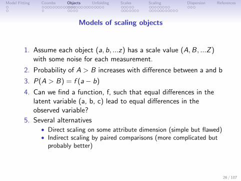
Models of scaling objects

1. Assume each object (a, b, ...z) has a scale value (A,B, ...Z )with some noise for each measurement.

2. Probability of A > B increases with difference between a and b

3. P(A > B) = f (a− b)

4. Can we find a function, f, such that equal differences in thelatent variable (a, b, c) lead to equal differences in theobserved variable?

5. Several alternatives• Direct scaling on some attribute dimension (simple but flawed)• Indirect scaling by paired comparisons (more complicated but

probably better)

26 / 107


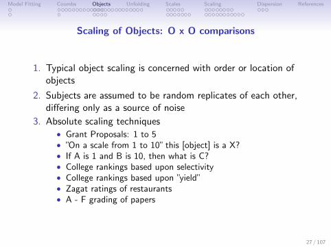
Scaling of Objects: O x O comparisons

1. Typical object scaling is concerned with order or location ofobjects

2. Subjects are assumed to be random replicates of each other,differing only as a source of noise

3. Absolute scaling techniques• Grant Proposals: 1 to 5• ”On a scale from 1 to 10” this [object] is a X?• If A is 1 and B is 10, then what is C?• College rankings based upon selectivity• College rankings based upon ”yield”• Zagat ratings of restaurants• A - F grading of papers

27 / 107


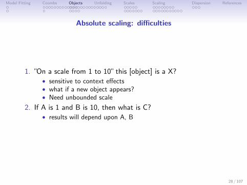
Absolute scaling: difficulties

1. ”On a scale from 1 to 10” this [object] is a X?• sensitive to context effects• what if a new object appears?• Need unbounded scale

2. If A is 1 and B is 10, then what is C?• results will depend upon A, B

28 / 107


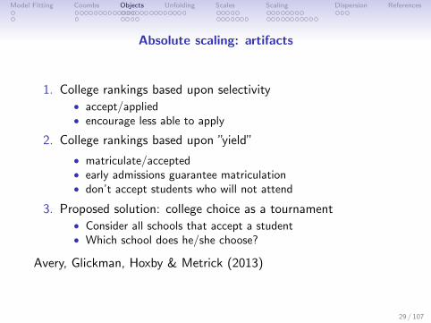
Absolute scaling: artifacts

1. College rankings based upon selectivity• accept/applied• encourage less able to apply

2. College rankings based upon ”yield”

• matriculate/accepted• early admissions guarantee matriculation• don’t accept students who will not attend

3. Proposed solution: college choice as a tournament• Consider all schools that accept a student• Which school does he/she choose?

Avery, Glickman, Hoxby & Metrick (2013)

29 / 107


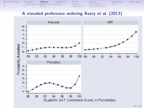
A revealed preference ordering Avery et al. (2013)

30 / 107


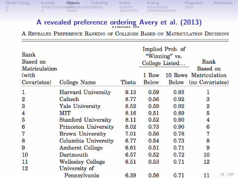
A revealed preference ordering Avery et al. (2013)

31 / 107


Weber-Fechner Law and non-linearity of scales

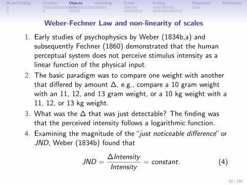
1. Early studies of psychophysics by Weber (1834b,a) andsubsequently Fechner (1860) demonstrated that the humanperceptual system does not perceive stimulus intensity as alinear function of the physical input.

2. The basic paradigm was to compare one weight with anotherthat differed by amount ∆, e.g., compare a 10 gram weightwith an 11, 12, and 13 gram weight, or a 10 kg weight with a11, 12, or 13 kg weight.

3. What was the ∆ that was just detectable? The finding wasthat the perceived intensity follows a logarithmic function.

4. Examining the magnitude of the “just noticeable difference” orJND, Weber (1834b) found that

JND =∆Intensity

Intensity= constant. (4)

32 / 107


Weber-Fechner Law and non-linearity of scales

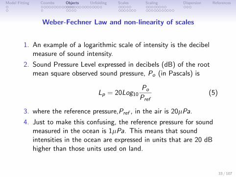
1. An example of a logarithmic scale of intensity is the decibelmeasure of sound intensity.

2. Sound Pressure Level expressed in decibels (dB) of the rootmean square observed sound pressure, Po (in Pascals) is

Lp = 20Log10Po

Pref(5)

3. where the reference pressure,Pref , in the air is 20µPa.

4. Just to make this confusing, the reference pressure for soundmeasured in the ocean is 1µPa. This means that soundintensities in the ocean are expressed in units that are 20 dBhigher than those units used on land.

33 / 107


The Just Noticeable Difference in Person perception

1. Although typically thought of as just relevant for theperceptual experiences of physical stimuli, Ozer (1993)suggested that the JND is useful in personality assessment asa way of understanding the accuracy and inter judgeagreement of judgments about other people.

2. In addition, Sinn (2003) has argued that the logarithmicnature of the Weber-Fechner Law is of evolutionarysignificance for preference for risk and cites Bernoulli (1738)as suggesting that our general utility function is logarithmic.

34 / 107


Money and non linearity

... the utility resulting from any small increase in wealthwill be inversely proportionate to the quantity of goodsalready possessed .... if ... one has a fortune worth ahundred thousand ducats and another one a fortuneworth same number of semi-ducats and if the formerreceives from it a yearly income of five thousand ducatswhile the latter obtains the same number of semi-ducats,it is quite clear that to the former a ducat has exactly thesame significance as a semi-ducat to the latter (Bernoulli,1738, p 25).

35 / 107


Thurstonian scaling: basic concept

1. Every object has a value

2. Rated strength of object is noisy with Gaussian noise

3. P(A > B) = f (za − zb)

4. Assume equal variance for each item

5. Convert choice frequency to normal deviates

6. Scale is average normal deviates

36 / 107


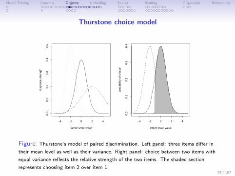
Thurstone choice model

−4 −2 0 2 4

0.0

0.1

0.2

0.3

0.4

0.5

latent scale value

resp

onse

str

engt

h

−4 −2 0 2 4

0.0

0.1

0.2

0.3

0.4

latent scale value

prob

abili

ty o

f cho

ice

Figure: Thurstone’s model of paired discrimination. Left panel: three items differ in

their mean level as well as their variance. Right panel: choice between two items with

equal variance reflects the relative strength of the two items. The shaded section

represents choosing item 2 over item 1.37 / 107


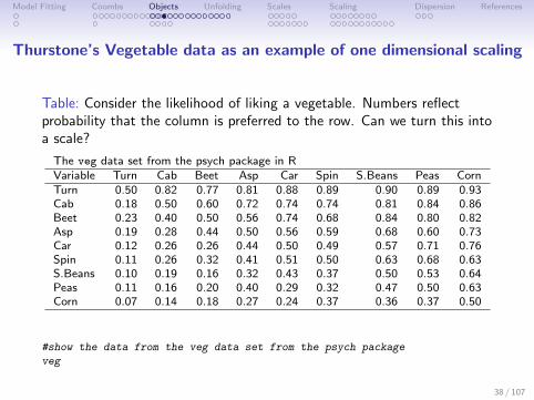
Thurstone’s Vegetable data as an example of one dimensional scaling

Table: Consider the likelihood of liking a vegetable. Numbers reflectprobability that the column is preferred to the row. Can we turn this intoa scale?

The veg data set from the psych package in RVariable Turn Cab Beet Asp Car Spin S.Beans Peas CornTurn 0.50 0.82 0.77 0.81 0.88 0.89 0.90 0.89 0.93Cab 0.18 0.50 0.60 0.72 0.74 0.74 0.81 0.84 0.86Beet 0.23 0.40 0.50 0.56 0.74 0.68 0.84 0.80 0.82Asp 0.19 0.28 0.44 0.50 0.56 0.59 0.68 0.60 0.73Car 0.12 0.26 0.26 0.44 0.50 0.49 0.57 0.71 0.76Spin 0.11 0.26 0.32 0.41 0.51 0.50 0.63 0.68 0.63S.Beans 0.10 0.19 0.16 0.32 0.43 0.37 0.50 0.53 0.64Peas 0.11 0.16 0.20 0.40 0.29 0.32 0.47 0.50 0.63Corn 0.07 0.14 0.18 0.27 0.24 0.37 0.36 0.37 0.50

#show the data from the veg data set from the psych package

veg

38 / 107


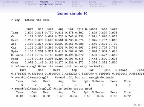
Some simple R

> veg #shows the data

Turn Cab Beet Asp Car Spin S.Beans Peas Corn

Turn 0.500 0.818 0.770 0.811 0.878 0.892 0.899 0.892 0.926

Cab 0.182 0.500 0.601 0.723 0.743 0.736 0.811 0.845 0.858

Beet 0.230 0.399 0.500 0.561 0.736 0.676 0.845 0.797 0.818

Asp 0.189 0.277 0.439 0.500 0.561 0.588 0.676 0.601 0.730

Car 0.122 0.257 0.264 0.439 0.500 0.493 0.574 0.709 0.764

Spin 0.108 0.264 0.324 0.412 0.507 0.500 0.628 0.682 0.628

S.Beans 0.101 0.189 0.155 0.324 0.426 0.372 0.500 0.527 0.642

Peas 0.108 0.155 0.203 0.399 0.291 0.318 0.473 0.500 0.628

Corn 0.074 0.142 0.182 0.270 0.236 0.372 0.358 0.372 0.500

> colMeans(veg) #show the means (but too many decimals)


0.1793333 0.3334444 0.3820000 0.4932222 0.5420000 0.5496667 0.6404444 0.6583333 0.7215556

> round(colMeans(veg)) #round off, but not enough decimals


0 0 0 0 1 1 1 1 1

> round(colMeans(veg),2) #this looks pretty good


0.18 0.33 0.38 0.49 0.54 0.55 0.64 0.66 0.72

39 / 107


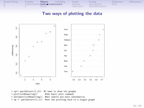
Two ways of plotting the data

2 4 6 8

0.2

0.3

0.4

0.5

0.6

0.7

Index

colMeans(veg)

Turn

Cab

Beet

Asp

Car

Spin

S.Beans

Peas

Corn

0.2 0.3 0.4 0.5 0.6 0.7

> op<- par(mfrow=c(1,2)) #I want to draw two graphs

> plot(colMeans(veg)) #the basic plot command

> dotchart(colMeans(veg)) #dot charts are more informative

> op <- par(mfrow=c(1,1)) #set the plotting back to a single graph

40 / 107


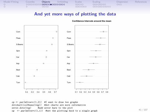
And yet more ways of plotting the data

Turn

Cab

Beet

Asp

Car

Spin

S.Beans

Peas

Corn

0.2 0.3 0.4 0.5 0.6 0.7

Turn

Cab

Beet

Asp

Car

Spin

S.Beans

Peas

Corn

0.1 0.2 0.3 0.4 0.5 0.6 0.7 0.8

Confidence Intervals around the mean

op <- par(mfrow=c(1,2)) #I want to draw two graphs

dotchart(colMeans(veg)) #dot charts are more informative

error.dots(veg) #add error bars to the plot

op <- par(mfrow=c(1,1)) #set the plotting back to a single graph 41 / 107


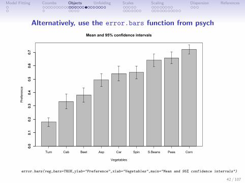
Alternatively, use the error.bars function from psych

Mean and 95% confidence intervals

Vegetables

Preference

0.0

0.1

0.2

0.3

0.4

0.5

0.6

0.7


0.0

0.1

0.2

0.3

0.4

0.5

0.6

0.7

error.bars(veg,bars=TRUE,ylab="Preference",xlab="Vegetables",main="Mean and 95% confidence intervals")

42 / 107


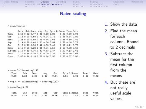
Naive scaling

> round(veg,2)


Turn 0.50 0.82 0.77 0.81 0.88 0.89 0.90 0.89 0.93

Cab 0.18 0.50 0.60 0.72 0.74 0.74 0.81 0.84 0.86

Beet 0.23 0.40 0.50 0.56 0.74 0.68 0.84 0.80 0.82

Asp 0.19 0.28 0.44 0.50 0.56 0.59 0.68 0.60 0.73

Car 0.12 0.26 0.26 0.44 0.50 0.49 0.57 0.71 0.76

Spin 0.11 0.26 0.32 0.41 0.51 0.50 0.63 0.68 0.63

S.Beans 0.10 0.19 0.16 0.32 0.43 0.37 0.50 0.53 0.64

Peas 0.11 0.16 0.20 0.40 0.29 0.32 0.47 0.50 0.63

Corn 0.07 0.14 0.18 0.27 0.24 0.37 0.36 0.37 0.50

> round(colMeans(veg),2)


0.18 0.33 0.38 0.49 0.54 0.55 0.64 0.66 0.72

> veg.t <- colMeans(veg) - mean(veg[,1])

> round(veg.t,2)


0.00 0.15 0.20 0.31 0.36 0.37 0.46 0.48 0.54

1. Show the data

2. Find the meanfor eachcolumn. Roundto 2 decimals

3. Subtract themean for thefirst columnfrom themeans

4. But these arenot reallyuseful scalevalues.

43 / 107


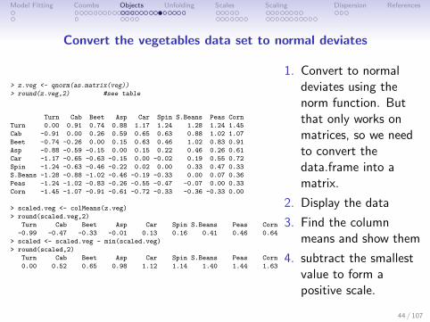
Convert the vegetables data set to normal deviates

> z.veg <- qnorm(as.matrix(veg))

> round(z.veg,2) #see table


Turn 0.00 0.91 0.74 0.88 1.17 1.24 1.28 1.24 1.45

Cab -0.91 0.00 0.26 0.59 0.65 0.63 0.88 1.02 1.07

Beet -0.74 -0.26 0.00 0.15 0.63 0.46 1.02 0.83 0.91

Asp -0.88 -0.59 -0.15 0.00 0.15 0.22 0.46 0.26 0.61

Car -1.17 -0.65 -0.63 -0.15 0.00 -0.02 0.19 0.55 0.72

Spin -1.24 -0.63 -0.46 -0.22 0.02 0.00 0.33 0.47 0.33

S.Beans -1.28 -0.88 -1.02 -0.46 -0.19 -0.33 0.00 0.07 0.36

Peas -1.24 -1.02 -0.83 -0.26 -0.55 -0.47 -0.07 0.00 0.33

Corn -1.45 -1.07 -0.91 -0.61 -0.72 -0.33 -0.36 -0.33 0.00

> scaled.veg <- colMeans(z.veg)

> round(scaled.veg,2)


-0.99 -0.47 -0.33 -0.01 0.13 0.16 0.41 0.46 0.64

> scaled <- scaled.veg - min(scaled.veg)

> round(scaled,2)


0.00 0.52 0.65 0.98 1.12 1.14 1.40 1.44 1.63

1. Convert to normaldeviates using thenorm function. Butthat only works onmatrices, so we needto convert thedata.frame into amatrix.

2. Display the data

3. Find the columnmeans and show them

4. subtract the smallestvalue to form apositive scale.

44 / 107


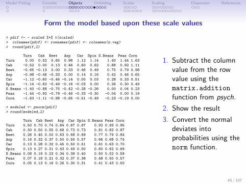
Form the model based upon these scale values

> pdif <- - scaled %+% t(scaled)

> colnames(pdif) <- rownames(pdif) <- colnames(z.veg)

> round(pdif,2)


Turn 0.00 0.52 0.65 0.98 1.12 1.14 1.40 1.44 1.63

Cab -0.52 0.00 0.13 0.46 0.60 0.62 0.88 0.92 1.11

Beet -0.65 -0.13 0.00 0.33 0.46 0.49 0.75 0.79 0.98

Asp -0.98 -0.46 -0.33 0.00 0.14 0.16 0.42 0.46 0.65

Car -1.12 -0.60 -0.46 -0.14 0.00 0.03 0.28 0.33 0.51

Spin -1.14 -0.62 -0.49 -0.16 -0.03 0.00 0.26 0.30 0.49

S.Beans -1.40 -0.88 -0.75 -0.42 -0.28 -0.26 0.00 0.04 0.23

Peas -1.44 -0.92 -0.79 -0.46 -0.33 -0.30 -0.04 0.00 0.19

Corn -1.63 -1.11 -0.98 -0.65 -0.51 -0.49 -0.23 -0.19 0.00

> modeled <- pnorm(pdif)

> round(modeled,2)


Turn 0.50 0.70 0.74 0.84 0.87 0.87 0.92 0.93 0.95

Cab 0.30 0.50 0.55 0.68 0.72 0.73 0.81 0.82 0.87

Beet 0.26 0.45 0.50 0.63 0.68 0.69 0.77 0.79 0.84

Asp 0.16 0.32 0.37 0.50 0.55 0.57 0.66 0.68 0.74

Car 0.13 0.28 0.32 0.45 0.50 0.51 0.61 0.63 0.70

Spin 0.13 0.27 0.31 0.43 0.49 0.50 0.60 0.62 0.69

S.Beans 0.08 0.19 0.23 0.34 0.39 0.40 0.50 0.52 0.59

Peas 0.07 0.18 0.21 0.32 0.37 0.38 0.48 0.50 0.57

Corn 0.05 0.13 0.16 0.26 0.30 0.31 0.41 0.43 0.50

1. Subtract the columnvalue from the rowvalue using thematrix.addition

function from psych.

2. Show the result

3. Convert the normaldeviates intoprobabilities using thenorm function.

45 / 107


Data = Model + Residual

1. What is the model?• Pref = Mean (preference)• p(A > B) = f (A,B)• what is f?

2. Possible functions• f = A - B (simple difference)• A

A+B Luce choice rule• Thurstonian scaling• logistic scaling

3. Evaluating functions – Goodness of fit• Residual = Model - Data• Minimize residual• Minimize residual2

46 / 107


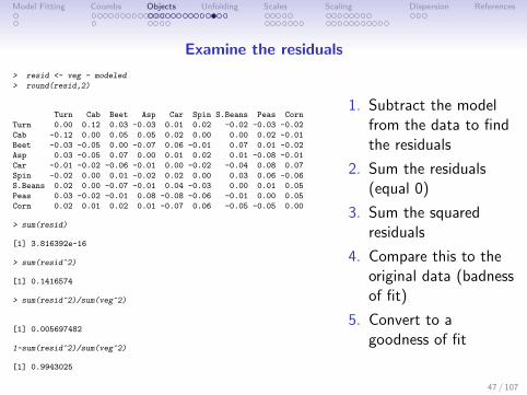
Examine the residuals

> resid <- veg - modeled

> round(resid,2)


Turn 0.00 0.12 0.03 -0.03 0.01 0.02 -0.02 -0.03 -0.02

Cab -0.12 0.00 0.05 0.05 0.02 0.00 0.00 0.02 -0.01

Beet -0.03 -0.05 0.00 -0.07 0.06 -0.01 0.07 0.01 -0.02

Asp 0.03 -0.05 0.07 0.00 0.01 0.02 0.01 -0.08 -0.01

Car -0.01 -0.02 -0.06 -0.01 0.00 -0.02 -0.04 0.08 0.07

Spin -0.02 0.00 0.01 -0.02 0.02 0.00 0.03 0.06 -0.06

S.Beans 0.02 0.00 -0.07 -0.01 0.04 -0.03 0.00 0.01 0.05

Peas 0.03 -0.02 -0.01 0.08 -0.08 -0.06 -0.01 0.00 0.05

Corn 0.02 0.01 0.02 0.01 -0.07 0.06 -0.05 -0.05 0.00

> sum(resid)

[1] 3.816392e-16

> sum(resid^2)

[1] 0.1416574

> sum(resid^2)/sum(veg^2)

[1] 0.005697482

1-sum(resid^2)/sum(veg^2)

[1] 0.9943025

1. Subtract the modelfrom the data to findthe residuals

2. Sum the residuals(equal 0)

3. Sum the squaredresiduals

4. Compare this to theoriginal data (badnessof fit)

5. Convert to agoodness of fit

47 / 107


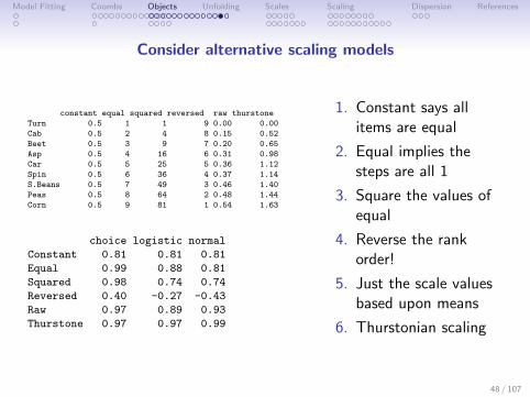
Consider alternative scaling models

constant equal squared reversed raw thurstone

Turn 0.5 1 1 9 0.00 0.00

Cab 0.5 2 4 8 0.15 0.52

Beet 0.5 3 9 7 0.20 0.65

Asp 0.5 4 16 6 0.31 0.98

Car 0.5 5 25 5 0.36 1.12

Spin 0.5 6 36 4 0.37 1.14

S.Beans 0.5 7 49 3 0.46 1.40

Peas 0.5 8 64 2 0.48 1.44

Corn 0.5 9 81 1 0.54 1.63

choice logistic normal

Constant 0.81 0.81 0.81

Equal 0.99 0.88 0.81

Squared 0.98 0.74 0.74

Reversed 0.40 -0.27 -0.43

Raw 0.97 0.89 0.93

Thurstone 0.97 0.97 0.99

1. Constant says allitems are equal

2. Equal implies thesteps are all 1

3. Square the values ofequal

4. Reverse the rankorder!

5. Just the scale valuesbased upon means

6. Thurstonian scaling

48 / 107


Thurstonian scaling as an example of model fitting

We don’t really care all that much about vegetables, but we docare about the process of model fitting.

1. Examine the data

2. Specify a model

3. Estimate the model

4. Compare the model to the data

5. Repeat until satisfied or exhausted

49 / 107


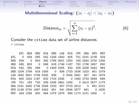
Multidimensional Scaling: (|oi − oj | < |ok − ol |)

Distancexy =

√√√√ n∑i=1

(xi − yi )2. (6)

Consider the cities data set of airline distances.> cities

ATL BOS ORD DCA DEN LAX MIA JFK SEA SFO MSY

ATL 0 934 585 542 1209 1942 605 751 2181 2139 424

BOS 934 0 853 392 1769 2601 1252 183 2492 2700 1356

ORD 585 853 0 598 918 1748 1187 720 1736 1857 830

DCA 542 392 598 0 1493 2305 922 209 2328 2442 964

DEN 1209 1769 918 1493 0 836 1723 1636 1023 951 1079

LAX 1942 2601 1748 2305 836 0 2345 2461 957 341 1679

MIA 605 1252 1187 922 1723 2345 0 1092 2733 2594 669

JFK 751 183 720 209 1636 2461 1092 0 2412 2577 1173

SEA 2181 2492 1736 2328 1023 957 2733 2412 0 681 2101

SFO 2139 2700 1857 2442 951 341 2594 2577 681 0 1925

MSY 424 1356 830 964 1079 1679 669 1173 2101 1925 0

50 / 107


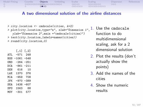
A two dimensional solution of the airline distances

> city.location <- cmdscale(cities, k=2)

> plot(city.location,type="n", xlab="Dimension 1",

ylab="Dimension 2",main ="cmdscale(cities)")

> text(city.location,labels=names(cities))

> round(city.location,0)

[,1] [,2]

ATL -571 248

BOS -1061 -548

ORD -264 -251

DCA -861 -211

DEN 616 10

LAX 1370 376

MIA -959 708

JFK -970 -389

SEA 1438 -607

SFO 1563 88

MSY -301 577

1. Use the cmdscale

function to domultidimensionalscaling, ask for a 2dimensional solution

2. Plot the results (don’tactually show thepoints)

3. Add the names of thecities

4. Show the numericresults

51 / 107


Original solution for 11 US cities. What is wrong with this figure?Axes of solutions are not necessarily directly interpretable.

-1000 -500 0 500 1000 1500

-600

-200

0200400600

Dimension 1

Dim

ensi

on 2 ATL

BOS

ORDDCA

DEN

LAX

MIA

JFK

SEA

SFO

MSY

Multidimensional Scaling of 11 cities

52 / 107


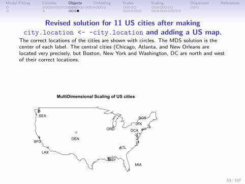
Revised solution for 11 US cities after makingcity.location <- -city.location and adding a US map.

The correct locations of the cities are shown with circles. The MDS solution is thecenter of each label. The central cities (Chicago, Atlanta, and New Orleans arelocated very precisely, but Boston, New York and Washington, DC are north and westof their correct locations.

MultiDimensional Scaling of US cities

ATL

BOS

ORD DCA

DEN

LAX

MIA

JFK

SEA

SFO

MSY

53 / 107


Preferential Choice: Unfolding Theory (|si − oj | < |sk − ol |)

1. “Do I like asparagus more than you like broccoli?” compareshow far apart my ideal vegetable is to a particular vegetable(asparagus) with respect to how far your ideal vegetable is toanother vegetable (broccoli).

2. More typical is the question of whether you like asparagusmore than you like broccoli. This comparison is between yourideal point (on an attribute dimension) to two objects on thatdimension.

3. Although the comparisons are ordinal, there is a surprisingamount of metric information in the analysis.

4. This involves unfolding the individual preference orderings tofind a joint scale of individuals and stimuli (Coombs, 1964,1975).

5. Can now be done using multidimensional scaling of people andobjects using proximity measures.

54 / 107


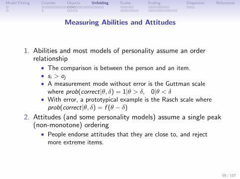
Measuring Abilities and Attitudes

1. Abilities and most models of personality assume an orderrelationship

• The comparison is between the person and an item.• si > oj

• A measurement mode without error is the Guttman scalewhere prob(correct|θ, δ) = 1|θ > δ, 0|θ < δ

• With error, a prototypical example is the Rasch scale whereprob(correct|θ, δ) = f (θ − δ)

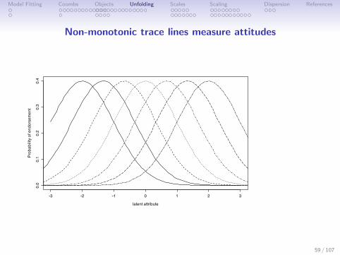
2. Attitudes (and some personality models) assume a single peak(non-monotone) ordering

• People endorse attitudes that they are close to, and rejectmore extreme items.

55 / 107


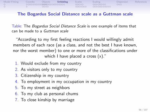
The Bogardus Social Distance scale as a Guttman scale

Table: The Bogardus Social Distance Scale is one example of items thatcan be made to a Guttman scale

“According to my first feeling reactions I would willingly admitmembers of each race (as a class, and not the best I have known,nor the worst member) to one or more of the classifications under

which I have placed a cross (x).”

1. Would exclude from my country

2. As visitors only to my country

3. Citizenship in my country

4. To employment in my occupation in my country

5. To my street as neighbors

6. To my club as personal chums

7. To close kinship by marriage

56 / 107


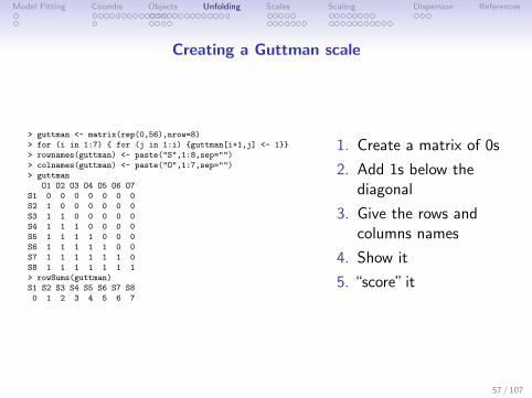
Creating a Guttman scale

> guttman <- matrix(rep(0,56),nrow=8)

> for (i in 1:7) { for (j in 1:i) {guttman[i+1,j] <- 1}}

> rownames(guttman) <- paste("S",1:8,sep="")

> colnames(guttman) <- paste("O",1:7,sep="")

> guttman

O1 O2 O3 O4 O5 O6 O7

S1 0 0 0 0 0 0 0

S2 1 0 0 0 0 0 0

S3 1 1 0 0 0 0 0

S4 1 1 1 0 0 0 0

S5 1 1 1 1 0 0 0

S6 1 1 1 1 1 0 0

S7 1 1 1 1 1 1 0

S8 1 1 1 1 1 1 1

> rowSums(guttman)

S1 S2 S3 S4 S5 S6 S7 S8

0 1 2 3 4 5 6 7

1. Create a matrix of 0s

2. Add 1s below thediagonal

3. Give the rows andcolumns names

4. Show it

5. “score” it

57 / 107


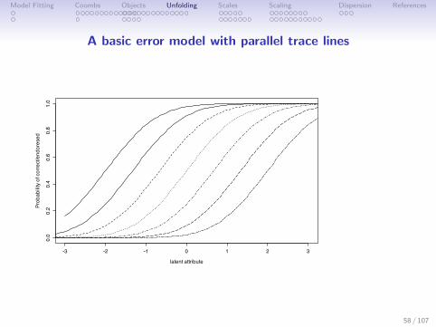
A basic error model with parallel trace lines

-3 -2 -1 0 1 2 3

0.0

0.2

0.4

0.6

0.8

1.0

latent attribute

Pro

ba

bility o

f co

rre

ct/e

nd

ore

se

d

58 / 107


Non-monotonic trace lines measure attitudes

-3 -2 -1 0 1 2 3

0.0

0.1

0.2

0.3

0.4

latent attribute

Pro

ba

bility o

f e

nd

ors

em

en

t

59 / 107


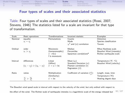
Four types of scales and their associated statistics

Table: Four types of scales and their associated statistics (Rossi, 2007;Stevens, 1946) The statistics listed for a scale are invariant for that typeof transformation.

Scale Basic operations Transformations Invariant statistic ExamplesNominal equality Permutations Counts Detection

xi = xj Mode Species classification

χ2 and (φ) correlation Taxons

Ordinal order Monotonic Median Mhos Hardness scalexi > xj (homeomorphic) Percentiles Beaufort Wind (intensity)

x’ =f(x) Spearman correlations* Richter earthquake scalef is monotonic

Interval differences Linear Mean (µ) Temperature (°F, °C)(Affine) Standard Deviation (σ) Beaufort Wind (velocity)

(xi − xj ) > (xk − xl ) x’ = a + bx Pearson correlation (r)Regression (β)

Ratio ratios Multiplication Coefficient of variation ( σµ

) Length, mass, time

(Similiarity) Temperature (°K)xixj>

xkxl

x’ = bx Heating degree days

The Beaufort wind speed scale is interval with respect to the velocity of the wind, but only ordinal with respect to

the effect of the wind. The Richter scale of earthquake intensity is a logarithmic scale of the energy released but

linear measure of the deflection on a seismometer.

60 / 107


Graphical and tabular summaries of data

1. The Tukey 5 number summary shows the importantcharacteristics of a set of numbers

• Maximum• 75th percentile• Median (50th percentile)• 25th percentile• Minimum

2. Graphically, this is the box plot• Variations on the box plot include confidence intervals for the

median

61 / 107


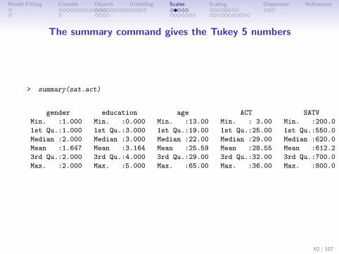
The summary command gives the Tukey 5 numbers

> summary(sat.act)

gender education age ACT SATV SATQ

Min. :1.000 Min. :0.000 Min. :13.00 Min. : 3.00 Min. :200.0 Min. :200.0

1st Qu.:1.000 1st Qu.:3.000 1st Qu.:19.00 1st Qu.:25.00 1st Qu.:550.0 1st Qu.:530.0

Median :2.000 Median :3.000 Median :22.00 Median :29.00 Median :620.0 Median :620.0

Mean :1.647 Mean :3.164 Mean :25.59 Mean :28.55 Mean :612.2 Mean :610.2

3rd Qu.:2.000 3rd Qu.:4.000 3rd Qu.:29.00 3rd Qu.:32.00 3rd Qu.:700.0 3rd Qu.:700.0

Max. :2.000 Max. :5.000 Max. :65.00 Max. :36.00 Max. :800.0 Max. :800.0

NA's :13

62 / 107


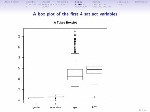
A box plot of the first 4 sat.act variables

gender education age ACT

010

2030

4050

60A Tukey Boxplot

boxplot(sat.act[1:4],main=”A Tukey Boxplot”)

63 / 107


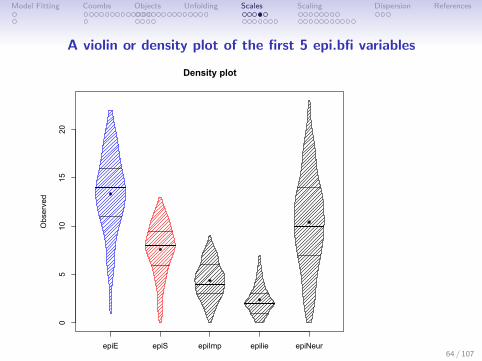
A violin or density plot of the first 5 epi.bfi variables

Density plot

Observed

epiE epiS epiImp epilie epiNeur

05

1015

20

violinBy(epi.bfi[1:5],main=”A Tukey violin plot”)

64 / 107


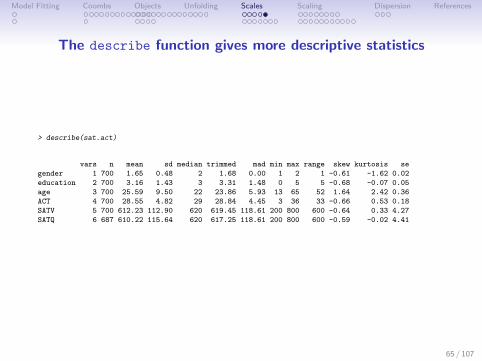
The describe function gives more descriptive statistics

> describe(sat.act)

vars n mean sd median trimmed mad min max range skew kurtosis se

gender 1 700 1.65 0.48 2 1.68 0.00 1 2 1 -0.61 -1.62 0.02

education 2 700 3.16 1.43 3 3.31 1.48 0 5 5 -0.68 -0.07 0.05

age 3 700 25.59 9.50 22 23.86 5.93 13 65 52 1.64 2.42 0.36

ACT 4 700 28.55 4.82 29 28.84 4.45 3 36 33 -0.66 0.53 0.18

SATV 5 700 612.23 112.90 620 619.45 118.61 200 800 600 -0.64 0.33 4.27

SATQ 6 687 610.22 115.64 620 617.25 118.61 200 800 600 -0.59 -0.02 4.41

65 / 107


Multiple measures of central tendency

mode The most frequent observation. Not a very stablemeasure, depends upon grouping. Can be used forcategorical data.

median The number with 50% above and 50% below. Apowerful, if underused, measure. Not sensitive totransforms of the shape of the distribution, noroutliers. Appropriate for ordinal data, and useful forinterval data.

mean One of at least seven measures that assume intervalproperties of the data.

66 / 107


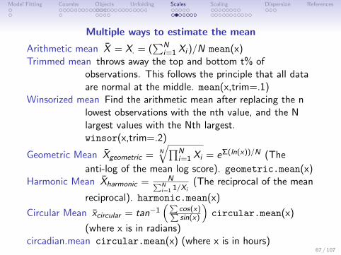
Multiple ways to estimate the mean

Arithmetic mean X̄ = X. = (∑N

i=1 Xi )/N mean(x)Trimmed mean throws away the top and bottom t% of

observations. This follows the principle that all dataare normal at the middle. mean(x,trim=.1)

Winsorized mean Find the arithmetic mean after replacing the nlowest observations with the nth value, and the Nlargest values with the Nth largest.winsor(x,trim=.2)

Geometric Mean X̄geometric = N

√∏Ni=1 Xi = eΣ(ln(x))/N (The

anti-log of the mean log score). geometric.mean(x)Harmonic Mean X̄harmonic = N∑N

i=1 1/Xi(The reciprocal of the mean

reciprocal). harmonic.mean(x)

Circular Mean x̄circular = tan−1(∑

cos(x)∑sin(x)

)circular.mean(x)

(where x is in radians)circadian.mean circular.mean(x) (where x is in hours)

67 / 107


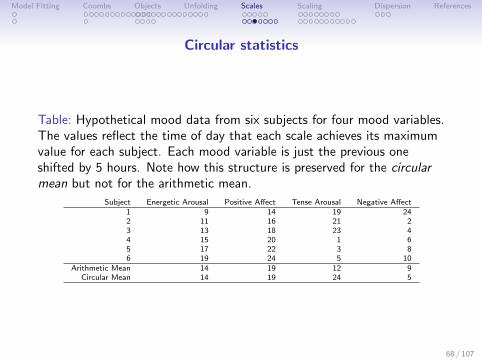
Circular statistics

Table: Hypothetical mood data from six subjects for four mood variables.The values reflect the time of day that each scale achieves its maximumvalue for each subject. Each mood variable is just the previous oneshifted by 5 hours. Note how this structure is preserved for the circularmean but not for the arithmetic mean.

Subject Energetic Arousal Positive Affect Tense Arousal Negative Affect1 9 14 19 242 11 16 21 23 13 18 23 44 15 20 1 65 17 22 3 86 19 24 5 10

Arithmetic Mean 14 19 12 9Circular Mean 14 19 24 5

68 / 107


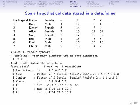
Some hypothetical data stored in a data.frame

Participant Name Gender θ X Y Z1 Bob Male 1 12 2 12 Debby Female 3 14 6 43 Alice Female 7 18 14 644 Gina Female 6 17 12 325 Eric Male 4 15 8 86 Fred Male 5 16 10 167 Chuck Male 2 13 4 2

> s.df <- read.clipboard()

> dim(s.df) #how many elements are in each dimension

[1] 7 7

> str(s.df) #show the structure

'data.frame': 7 obs. of 7 variables:

$ Participant: int 1 2 3 4 5 6 7

$ Name : Factor w/ 7 levels "Alice","Bob",..: 2 4 1 7 5 6 3

$ Gender : Factor w/ 2 levels "Female","Male": 2 1 1 1 2 2 2

$ theta : int 1 3 7 6 4 5 2

$ X : int 12 14 18 17 15 16 13

$ Y : num 2 6 14 12 8 10 4

$ Z : int 1 4 64 32 8 16 2

69 / 107


Saving the data.frame in a readable form

The previous slide is readable by humans, but harder to read bycomputer. PDFs are formatted in a rather weird way. We canshare data on slides by using the dput function. Copy this outputto your clipboard from the slide, and then get it into Rdirectly.> dput(sf.df)

structure(list(ID = 1:7, Name = structure(c(2L, 4L, 1L, 7L, 5L,

6L, 3L), .Label = c("Alice", "Bob", "Chuck", "Debby", "Eric",

"Fred", "Gina"), class = "factor"), gender = structure(c(2L,

1L, 1L, 1L, 2L, 2L, 2L), .Label = c("Female", "Male"), class = "factor"),

theta = c(1L, 3L, 7L, 6L, 4L, 5L, 2L), X = c(12L, 14L, 18L,

17L, 15L, 16L, 13L), Y = c(2L, 6L, 14L, 12L, 8L, 10L, 4L),

Z = c(1L, 4L, 64L, 32L, 8L, 16L, 2L)), .Names = c("ID", "Name",

"gender", "theta", "X", "Y", "Z"), class = "data.frame", row.names = c(NA,

-7L))

my.data <- structure(list(ID = 1:7, Name = structure(c(2L, 4L, 1L, 7L, 5L,

6L, 3L), .Label = c("Alice", "Bob", "Chuck", "Debby", "Eric",

"Fred", "Gina"), class = "factor"), gender = structure(c(2L,

1L, 1L, 1L, 2L, 2L, 2L), .Label = c("Female", "Male"), class = "factor"),

theta = c(1L, 3L, 7L, 6L, 4L, 5L, 2L), X = c(12L, 14L, 18L,

17L, 15L, 16L, 13L), Y = c(2L, 6L, 14L, 12L, 8L, 10L, 4L),

Z = c(1L, 4L, 64L, 32L, 8L, 16L, 2L)), .Names = c("ID", "Name",

"gender", "theta", "X", "Y", "Z"), class = "data.frame", row.names = c(NA,

-7L))

70 / 107


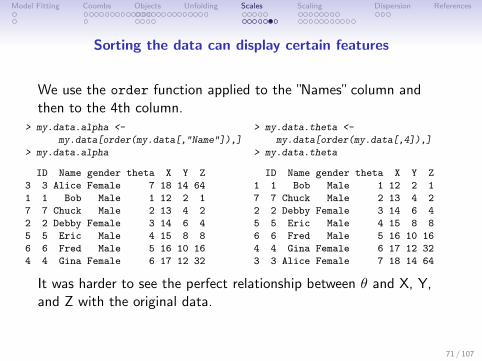
Sorting the data can display certain features

We use the order function applied to the ”Names” column andthen to the 4th column.

> my.data.alpha <-

my.data[order(my.data[,"Name"]),]

> my.data.alpha

ID Name gender theta X Y Z

3 3 Alice Female 7 18 14 64

1 1 Bob Male 1 12 2 1

7 7 Chuck Male 2 13 4 2

2 2 Debby Female 3 14 6 4

5 5 Eric Male 4 15 8 8

6 6 Fred Male 5 16 10 16

4 4 Gina Female 6 17 12 32

> my.data.theta <-

my.data[order(my.data[,4]),]

> my.data.theta

ID Name gender theta X Y Z

1 1 Bob Male 1 12 2 1

7 7 Chuck Male 2 13 4 2

2 2 Debby Female 3 14 6 4

5 5 Eric Male 4 15 8 8

6 6 Fred Male 5 16 10 16

4 4 Gina Female 6 17 12 32

3 3 Alice Female 7 18 14 64

It was harder to see the perfect relationship between θ and X, Y,and Z with the original data.

71 / 107


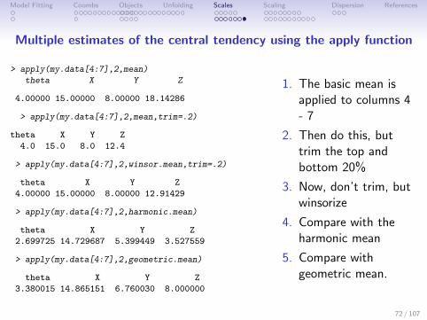
Multiple estimates of the central tendency using the apply function

> apply(my.data[4:7],2,mean)

theta X Y Z

4.00000 15.00000 8.00000 18.14286

> apply(my.data[4:7],2,mean,trim=.2)

theta X Y Z

4.0 15.0 8.0 12.4

> apply(my.data[4:7],2,winsor.mean,trim=.2)

theta X Y Z

4.00000 15.00000 8.00000 12.91429

> apply(my.data[4:7],2,harmonic.mean)

theta X Y Z

2.699725 14.729687 5.399449 3.527559

> apply(my.data[4:7],2,geometric.mean)

theta X Y Z

3.380015 14.865151 6.760030 8.000000

1. The basic mean isapplied to columns 4- 7

2. Then do this, buttrim the top andbottom 20%

3. Now, don’t trim, butwinsorize

4. Compare with theharmonic mean

5. Compare withgeometric mean.

72 / 107


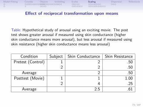
Effect of reciprocal transformation upon means

Table: Hypothetical study of arousal using an exciting movie. The posttest shows greater arousal if measured using skin conductance (higherskin conductance means more arousal), but less arousal if measured usingskin resistance (higher skin conductance means less arousal)

Condition Subject Skin Conductance Skin Resistance

Pretest (Control) 1 2 .502 2 .50

Average 2 .50

Posttest (Movie) 1 1 1.002 4 .25

Average 2.5 .61

73 / 107


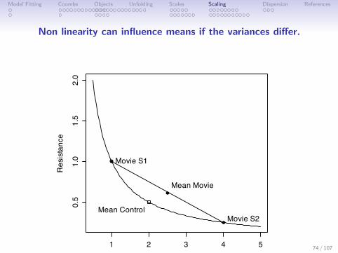
Non linearity can influence means if the variances differ.

1 2 3 4 5

0.5

1.0

1.5

2.0

Conductance

Re

sis

tan

ce

Mean Movie

Mean Control

Movie S2

Movie S1

Figure: The effect of non-linearity and variability on estimates of centraltendency. The movie condition increases the variability of the arousalmeasures. The “real effect” of the movie is to increase variability which ismistakenly interpreted as an increase/decrease in arousal.

74 / 107


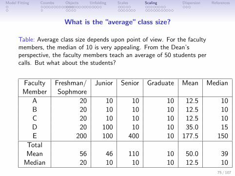
What is the ”average” class size?

Table: Average class size depends upon point of view. For the facultymembers, the median of 10 is very appealing. From the Dean’sperspective, the faculty members teach an average of 50 students percalls. But what about the students?

Faculty Freshman/ Junior Senior Graduate Mean MedianMember Sophmore

A 20 10 10 10 12.5 10B 20 10 10 10 12.5 10C 20 10 10 10 12.5 10D 20 100 10 10 35.0 15E 200 100 400 10 177.5 150

TotalMean 56 46 110 10 50.0 39

Median 20 10 10 10 12.5 10

75 / 107


Class size from the students’ point of view.

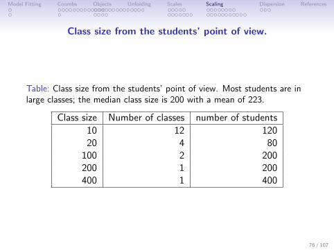
Table: Class size from the students’ point of view. Most students are inlarge classes; the median class size is 200 with a mean of 223.

Class size Number of classes number of students

10 12 12020 4 80

100 2 200200 1 200400 1 400

76 / 107


Time in therapy

A psychotherapist is asked what is the average length of time thata patient is in therapy. This seems to be an easy question, for ofthe 20 patients, 19 have been in therapy for between 6 and 18months (with a median of 12) and one has just started. Thus, themedian client is in therapy for 52 weeks with an average (in weeks)(1 * 1 + 19 * 52)/20 or 49.4.However, a more careful analysis examines the case load over ayear and discovers that indeed, 19 patients have a median time intreatment of 52 weeks, but that each week the therapist is alsoseeing a new client for just one session. That is, over the year, thetherapist sees 52 patients for 1 week and 19 for a median of 52weeks. Thus, the median client is in therapy for 1 week and theaverage client is in therapy of ( 52 * 1 + 19 * 52 )/(52+19) =14.6 weeks.

77 / 107


Does teaching effect learning?

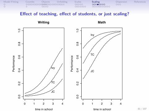
1. A leading research team in motivational and educationalpsychology was interested in the effect that different teachingtechniques at various colleges and universities have upon theirstudents. They were particularly interested in the effect uponwriting performance of attending a very selective university, aless selective university, or a two year junior college.

2. A writing test was given to the entering students at threeinstitutions in the Boston area. After one year, a similarwriting test was given again. Although there was someattrition from each sample, the researchers report data onlyfor those who finished one year. The pre and post test scoresas well as the change scores were as shown below:

78 / 107


Types of teaching affect student outcomes?

Table: Three types of teaching and their effect on student outcomes

School Pretest Posttest Change

Junior College 1 5 4Non-selective university 5 27 22Selective university 27 73 45

From these data, the researchers concluded that the quality ofteaching at the selective university was much better than that ofthe less selective university or the junior college and that thestudents learned a great deal more. They proposed to study thetechniques used there in order to apply them to the otherinstitutions.

79 / 107


Teaching and math performance

Another research team in motivational and educational psychologywas interested in the effect that different teaching at variouscolleges and universities affect math performance. They used thesame schools as the previous example with the same design.

Table: Three types of teaching and their effect on student outcomes

School Pretest Posttest Change

Junior College 27 73 45Non-selective university 73 95 22Selective university 95 99 4

They concluded that the teaching at the junior college was farsuperior to that of the select university. What is wrong with thisconclusion?

80 / 107


Effect of teaching, effect of students, or just scaling?

0 1 2 3 4

0.0

0.2

0.4

0.6

0.8

1.0

Writing

time in school

Pe

rfo

rma

nce

Ivy

JC

TC

0 1 2 3 4

0.0

0.2

0.4

0.6

0.8

1.0

Math

time in school

Pe

rfo

rma

nce

Ivy

JC

TC

81 / 107


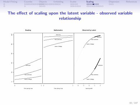
The effect of scaling upon the latent variable - observed variablerelationship

0 1

020

4060

8010

0

Reading

Time during Year

Junior College

Non selective

Selective

0 1

Mathematics

Time during Year

100/

(1 +

exp

(−x

− 2

))

Junior College

Non selective

Selective

−2 −1 0 1 2

Observed by Latent

latent growth

100/

(1 +

exp

(−x

− 2

))

Junior College

Non selective

Selective

Junior College

Non selective

Selective

82 / 107


The problem of scaling is ubiquitous

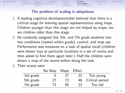
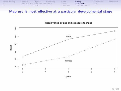
1. A leading cognitive developmentalist believed that there is acritiical stage for learning spatial representations using maps.Children younger than this stage are not helped by maps, norare children older than this stage.

2. He randomly assigned 3rd, 5th, and 7th grade students intotwo conditions (nested within grade), control, and map use.Performance was measures on a task of spatial recall (childrenwere shown toys at particular locations in a set of rooms andthen asked to find them again later.) Half the children wereshown a map of the rooms before doing the task.

3. Their scores were

No Map Maps Effect

3rd grade 5 27 22 Too young5th grade 27 73 46 Critical period7th grade 73 95 22 Too old

83 / 107


Map use is most effective at a particular developmental stage

3 4 5 6 7

020

4060

80100

Recall varies by age and exposure to maps

grade

Recall

maps

nomaps

84 / 107


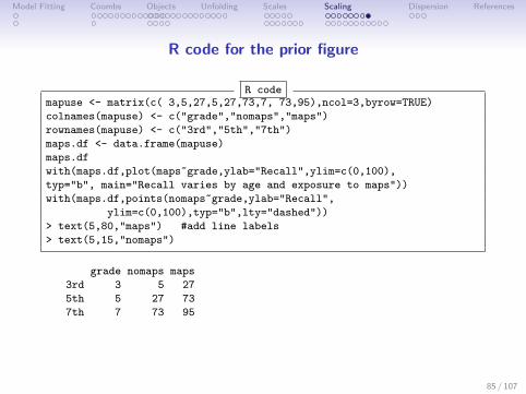
R code for the prior figure

R codemapuse <- matrix(c( 3,5,27,5,27,73,7, 73,95),ncol=3,byrow=TRUE)

colnames(mapuse) <- c("grade","nomaps","maps")

rownames(mapuse) <- c("3rd","5th","7th")

maps.df <- data.frame(mapuse)

maps.df

with(maps.df,plot(maps~grade,ylab="Recall",ylim=c(0,100),

typ="b", main="Recall varies by age and exposure to maps"))

with(maps.df,points(nomaps~grade,ylab="Recall",

ylim=c(0,100),typ="b",lty="dashed"))

> text(5,80,"maps") #add line labels

> text(5,15,"nomaps")

grade nomaps maps

3rd 3 5 27

5th 5 27 73

7th 7 73 95

85 / 107


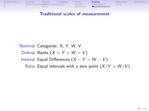
Traditional scales of measurement

Nominal Categories: X, Y, W, V

Ordinal Ranks (X > Y > W > V )

Interval Equal Differences (X − Y > W − V )

Ratio Equal intervals with a zero point (X/Y > W /V )

86 / 107


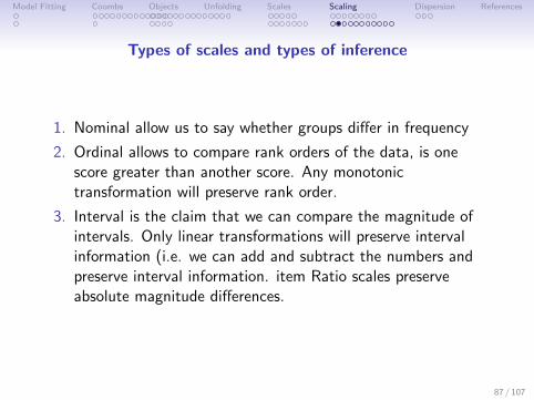
Types of scales and types of inference

1. Nominal allow us to say whether groups differ in frequency

2. Ordinal allows to compare rank orders of the data, is onescore greater than another score. Any monotonictransformation will preserve rank order.

3. Interval is the claim that we can compare the magnitude ofintervals. Only linear transformations will preserve intervalinformation (i.e. we can add and subtract the numbers andpreserve interval information. item Ratio scales preserveabsolute magnitude differences.

87 / 107


Ordinal scales

1. Any monotonic transformation will preserve order

2. Inferences from observed to latent variable are restricted torank orders

3. Statistics: Medians, Quartiles, Percentiles

88 / 107


Interval scales

1. Possible to infer the magnitude of differences between pointson the latent variable given differences on the observedvariable?X is as much greater than Y as Z is from W

2. Linear transformations preserve interval information

3. Allowable statistics: Means, Variances

4. Although our data are actually probably just ordinal, we tendto use interval assumptions.

89 / 107


Ratio Scales

1. Interval scales with a zero point

2. Possible to compare ratios of magnitudes (X is twice as longas Y)

3. Are there any psychological examples?

90 / 107


The search for an appropriate scale

1. Is today colder than yesterday? (ranks) Is the amount thattoday is colder than yesterday more than the amount thatyesterday was colder than the day before? (intervals)

• 50F − 39F < 68F − 50F• 10C − 4C < 20C − 10C• 283K − 277K < 293K − 283K

2. How much colder is today than yesterday?

• (Degree days as measure of energy use) is almost ratio• K as measure of molecular energy

91 / 107


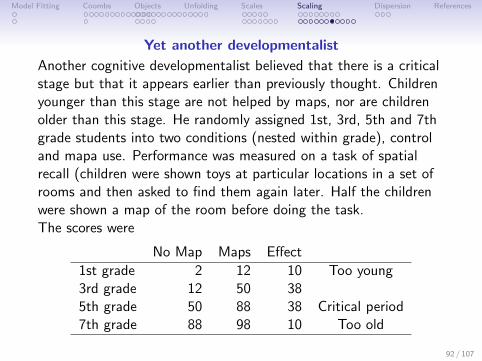
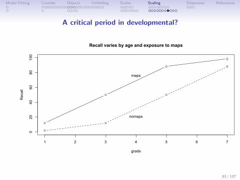
Yet another developmentalist

Another cognitive developmentalist believed that there is a criticalstage but that it appears earlier than previously thought. Childrenyounger than this stage are not helped by maps, nor are childrenolder than this stage. He randomly assigned 1st, 3rd, 5th and 7thgrade students into two conditions (nested within grade), controland mapa use. Performance was measured on a task of spatialrecall (children were shown toys at particular locations in a set ofrooms and then asked to find them again later. Half the childrenwere shown a map of the room before doing the task.The scores were

No Map Maps Effect

1st grade 2 12 10 Too young3rd grade 12 50 385th grade 50 88 38 Critical period7th grade 88 98 10 Too old

92 / 107


A critical period in developmental?

1 2 3 4 5 6 7

020

4060

80100

Recall varies by age and exposure to maps

grade

Recall

maps

nomaps

93 / 107


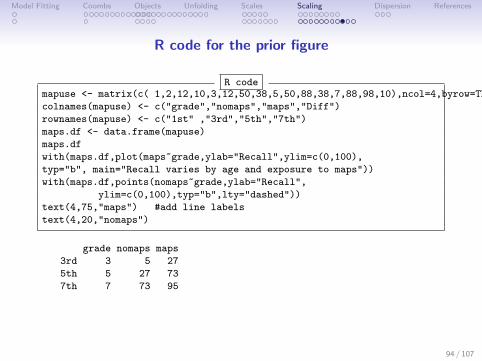
R code for the prior figure

R codemapuse <- matrix(c( 1,2,12,10,3,12,50,38,5,50,88,38,7,88,98,10),ncol=4,byrow=TRUE)

colnames(mapuse) <- c("grade","nomaps","maps","Diff")

rownames(mapuse) <- c("1st" ,"3rd","5th","7th")

maps.df <- data.frame(mapuse)

maps.df

with(maps.df,plot(maps~grade,ylab="Recall",ylim=c(0,100),

typ="b", main="Recall varies by age and exposure to maps"))

with(maps.df,points(nomaps~grade,ylab="Recall",

ylim=c(0,100),typ="b",lty="dashed"))

text(4,75,"maps") #add line labels

text(4,20,"nomaps")

grade nomaps maps

3rd 3 5 27

5th 5 27 73

7th 7 73 95

94 / 107


Measurement confusions – arousal

1. Arousal is a fundamental concept in many psychologicaltheories. It is thought to reflect basic levels of alertness andpreparedness. Typical indices of arousal are measures of theamount of palmer sweating.

2. This may be indexed by the amount of electricity that isconducted by the fingertips.

3. Alternatively, it may be indexed (negatively) by the amount ofskin resistance of the finger tips. The Galvanic Skin Response(GSR) reflects moment to moment changes, SC and SRreflect longer term, basal levels.

4. High skin conductance (low skin resistance) is thought toreflect high arousal.

95 / 107


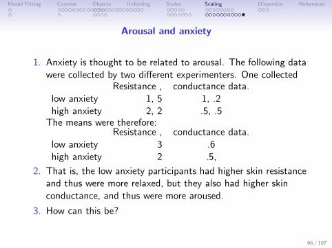
Arousal and anxiety

1. Anxiety is thought to be related to arousal. The following datawere collected by two different experimenters. One collected

Resistance , conductance data.low anxiety 1, 5 1, .2high anxiety 2, 2 .5, .5

The means were therefore:Resistance , conductance data.

low anxiety 3 .6high anxiety 2 .5,

2. That is, the low anxiety participants had higher skin resistanceand thus were more relaxed, but they also had higher skinconductance, and thus were more aroused.

3. How can this be?

96 / 107


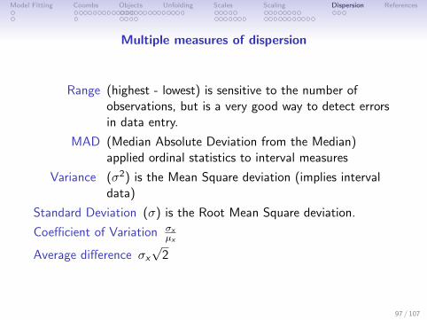
Multiple measures of dispersion

Range (highest - lowest) is sensitive to the number ofobservations, but is a very good way to detect errorsin data entry.

MAD (Median Absolute Deviation from the Median)applied ordinal statistics to interval measures

Variance (σ2) is the Mean Square deviation (implies intervaldata)

Standard Deviation (σ) is the Root Mean Square deviation.

Coefficient of Variation σxµx

Average difference σx√

2

97 / 107


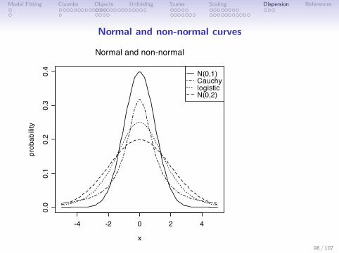
Normal and non-normal curves

-4 -2 0 2 4

0.0

0.1

0.2

0.3

0.4

x

pro

ba

bility

N(0,1)CauchylogisticN(0,2)

Normal and non-normal

98 / 107


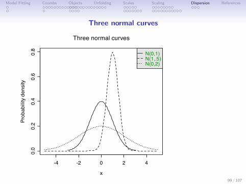
Three normal curves

-4 -2 0 2 4

0.0

0.2

0.4

0.6

0.8

x

Prob

abili

ty d

ensi

ty

N(0,1)N(1,.5)N(0,2)

Three normal curves

99 / 107


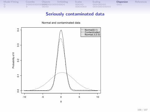
Seriously contaminated data

-10 -5 0 5 10

0.0

0.1

0.2

0.3

0.4

X

Pro

ba

bility o

f X

Normal and contaminated data

Normal(0,1)ContaminatedNormal(.3,3.3)

100 / 107


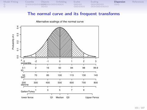
The normal curve and its frequent transforms

-3 -2 -1 0 1 2 3

0.0

0.1

0.2

0.3

0.4

Pro

ba

bility o

f z

0.1 2 16 50 84 98 99.9

55 70 85 100 115 130 145

200 300 400 500 600 700 800

lower fence Q1 Median Q3 Upper Fence

1 3 5 7 9

Alternative scalings of the normal curve

z

percentile

IQ

SAT

Galton/Tukey

stanine

101 / 107


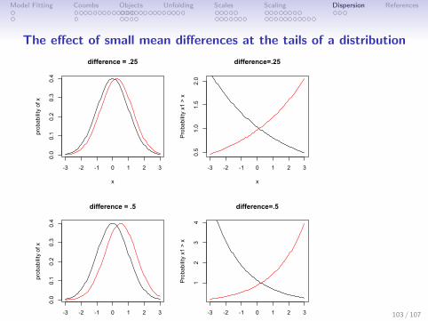
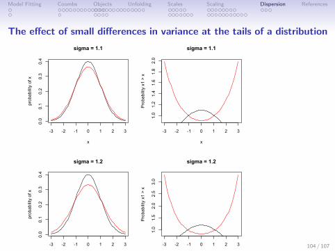
Decision making and the benefit of extreme selection ratios

1. Typical traits are approximated by a normal distribution.

2. Small differences in means or variances can lead to largedifferences in relative odds at the tails

3. Accuracy of decision/prediction is higher for extreme values.

4. Do we infer trait mean differences from observing differencesof extreme values?

102 / 107


The effect of small mean differences at the tails of a distribution

-3 -2 -1 0 1 2 3

0.0

0.1

0.2

0.3

0.4

difference = .25

x

prob

abili

ty o

f x

-3 -2 -1 0 1 2 3

0.5

1.0

1.5

2.0

difference=.25

xP

roba

bilit

y x1

> x

-3 -2 -1 0 1 2 3

0.0

0.1

0.2

0.3

0.4

difference = .5

x

prob

abili

ty o

f x

-3 -2 -1 0 1 2 3

12

34

difference=.5

x

Pro

babi

lity

x1 >

x

103 / 107


The effect of small differences in variance at the tails of a distribution

-3 -2 -1 0 1 2 3

0.0

0.1

0.2

0.3

0.4

sigma = 1.1

x

prob

abili

ty o

f x

-3 -2 -1 0 1 2 3

1.0

1.2

1.4

1.6

1.8

2.0

sigma = 1.1

xP

roba

bilit

y x1

> x

-3 -2 -1 0 1 2 3

0.0

0.1

0.2

0.3

0.4

sigma = 1.2

x

prob

abili

ty o

f x

-3 -2 -1 0 1 2 3

1.0

1.5

2.0

2.5

3.0

sigma = 1.2

x

Pro

babi

lity

x1 >

x

104 / 107


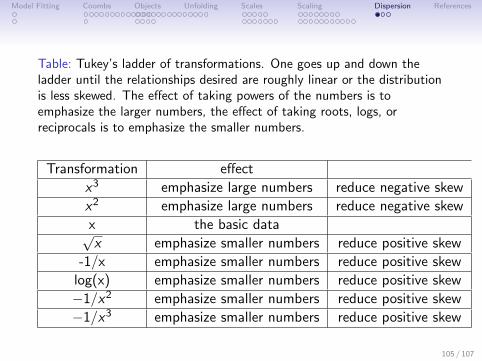
Table: Tukey’s ladder of transformations. One goes up and down theladder until the relationships desired are roughly linear or the distributionis less skewed. The effect of taking powers of the numbers is toemphasize the larger numbers, the effect of taking roots, logs, orreciprocals is to emphasize the smaller numbers.

Transformation effect

x3 emphasize large numbers reduce negative skew

x2 emphasize large numbers reduce negative skew

x the basic data√x emphasize smaller numbers reduce positive skew

-1/x emphasize smaller numbers reduce positive skew

log(x) emphasize smaller numbers reduce positive skew

−1/x2 emphasize smaller numbers reduce positive skew

−1/x3 emphasize smaller numbers reduce positive skew

105 / 107


0.0 0.5 1.0 1.5 2.0

−2

−1

01

2

Tukey's ladder of transformations

original

tran

sfor

med

x^3x^2xsqrt(x)−1/xlog(x)−1/x^2−1/x^3

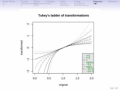
Figure: Tukey (1977) suggested a number of transformations of data thatallow relationships to be seen more easily. Ranging from the cube to thereciprocal of the cube, these transformations emphasize different parts ofthe distribution.

106 / 107


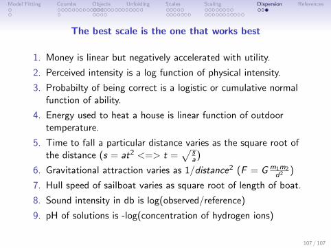
The best scale is the one that works best

1. Money is linear but negatively accelerated with utility.

2. Perceived intensity is a log function of physical intensity.

3. Probabilty of being correct is a logistic or cumulative normalfunction of ability.

4. Energy used to heat a house is linear function of outdoortemperature.

5. Time to fall a particular distance varies as the square root ofthe distance (s = at2 <=> t =

√sa)

6. Gravitational attraction varies as 1/distance2 (F = G m1m2d2 )

7. Hull speed of sailboat varies as square root of length of boat.

8. Sound intensity in db is log(observed/reference)

9. pH of solutions is -log(concentration of hydrogen ions)

107 / 107


Avery, C. N., Glickman, M. E., Hoxby, C. M., & Metrick, A.(2013). A revealed preference ranking of u.s. colleges anduniversities. The Quarterly Journal of Economics, 128(1),425–467.

Bernoulli, D. (1954/1738). Exposition of a new theory on themeasurement of risk (“Specimen theoriae novae de mensurasortis,” Commentarii Academiae Scientiarum ImperialisPetropolitanae 5, St. Petersburg 175-92.) translated by LouiseC. Sommer. Econometrica, 22(1), 23–36.

Burchard, U. (2004). The sclerometer and the determination ofthe hardness of minerals. Mineralogical Record, 35, 109–120.

Coombs, C. (1964). A Theory of Data. New York: John Wiley.

Coombs, C. (1975). A note on the relation between the vectormodel and the unfolding model for preferences. Psychometrika,40, 115–116.

Fechner, Gustav Theodor (H.E. Adler, T. (1966/1860). Elemente107 / 107


der Psychophysik (Elements of psychophysics). Leipzig:Breitkopf & Hartel.

Ozer, D. J. (1993). Classical psychophysics and the assessment ofagreement and accuracy in judgments of personality. Journal ofPersonality, 61(4), 739–767.

Rossi, G. B. (2007). Measurability. Measurement, 40(6), 545 –562.

Sinn, H. W. (2003). Weber’s law and the biological evolution ofrisk preferences: The selective dominance of the logarithmicutility function, 2002 geneva risk lecture. Geneva Papers on Riskand Insurance Theory, 28(2), 87–100.

Stevens, S. (1946). On the theory of scales of measurement.Science, 103(2684), 677–680.

Tukey, J. W. (1977). Exploratory data analysis. Reading, Mass.:Addison-Wesley Pub. Co.

Weber, E. H. (1834b). De pulsu, resorptione, auditu et tactu.Annotationes anatomicae et physiologicae. Leipzig: Kohler.

107 / 107


Weber, E. H. (1948/1834a). Concerning touch, 1834. InW. Dennis (Ed.), Readings in the history of psychology (pp.155–156). East Norwalk, CT: Appleton-Century-CroftsAppleton-Century-Crofts Print.

107 / 107

An introduction to Psychometric Theory Theory of Data ... fileAn introduction to Psychometric Theory...

Documents

Transcript of An introduction to Psychometric Theory Theory of Data ... fileAn introduction to Psychometric Theory...