An Introduction to Partial Equilibrium Modeling of Trade ... · AN INTRODUCTION TO PARTIAL...

1

AN INTRODUCTION TO PARTIAL EQUILIBRIUM

MODELING OF TRADE POLICY

Ross Hallren

David Riker

ECONOMICS WORKING PAPER SERIES

Working Paper 2017-07-B

U.S. INTERNATIONAL TRADE COMMISSION

500 E Street SW

Washington, DC 20436

July 2017

The authors are grateful to Andre Barbe, Justino De La Cruz and Craig Thomsen for helpful comments and suggestions.

Office of Economics working papers are the result of ongoing professional research of USITC Staff and are solely meant to represent the opinions and professional research of individual authors. These papers are not meant to represent in any way the views of the U.S. International Trade Commission or any of its individual Commissioners. Working papers are circulated to promote the active exchange of ideas between USITC Staff and recognized experts outside the USITC and to promote professional development of Office Staff by encouraging outside professional critique of staff research.

2

An Introduction to Partial Equilibrium Modeling of Trade Policy

Ross Hallren and David Riker Office of Economics Working Paper 2017-07-B July 2017

ABSTRACT

This paper introduces the theoretical framework and data inputs of a basic partial equilibrium

model of how an industry’s import volumes, domestic shipments, and prices would change in

response to a change in trade policy. We start with an overview of economic models used to

estimate the effects of tariffs and quotas on imports. Then we go step-by-step through the

equations that we use to calculate the changes in the economic outcomes and discuss the data

required to run the model. Next, we report several illustrative applications. We conclude with a

discussion of several extensions of the basic model.

Ross Hallren

Office of Economic, Research Division

[email protected]

David Riker

Office of Economics, Research Division

[email protected]

3

1. Introduction

An economic model is a system of equations that can be used to quantify the changes in economic

outcomes resulting from a change in policy. In this case, the economic outcomes that we analyze are

import volumes, domestic shipments, and prices in a specific industry and the policies are tariffs

and quotas on industry imports.

In trade policy analysis, models are often used to create forward-looking projections of the

economic effects of policy changes that have not yet occurred. Model-based simulations are well-

suited for this type of prospective analysis. Simulations isolate the effect of a trade policy by

changing the policy (e.g., the tariff rate), assuming that other supply and demand fundamentals do

not change. The parameters of the model are calibrated to current or recent data for the industry.

The economic impact of the policy is calculated as the difference between the model’s predictions

for market prices and quantities after the policy change and the baseline values of market prices

and quantities before (or absent) the policy change. In this paper, we focus on two common trade

policies: ad valorem tariffs and import quotas. 1

Simulation models of trade policy vary in complexity. Computable general equilibrium (CGE)

models are elaborate models that require a lot of data and are sometimes difficult to run, but they

are a very useful analytical tool when the policy changes under consideration affect many different

sectors in the economy and policy makers are requesting an estimate of economy-wide effects of

the policy changes. On the other hand, when the policy changes are more narrowly focused on a

single industry, smaller targeted industry-specific models can be the right tool because they are

easy to set up, modify, and operate, and they generally require fewer data inputs. This paper

introduces the basic industry-specific model.

1 An ad valorem tariff is a fixed percentage of the value of the imports rather than a specific dollar amount per unit of quantity. The model can also be modified to analyze specific tariffs.

4

We make a number of assumptions to simplify the equations in our industry-specific model. Chief

among these simplifications, we assume that aggregate expenditure levels and prices in other

industries in the economy do not change with the changes in trade policy. This partial equilibrium

approach is an appropriate simplification when the industry is only a small share of the overall

economy.

The rest of this paper is organized into four parts. Section 2 describes the equations and

assumptions of the model. Section 3 discusses the data inputs. Section 4 presents illustrative

applications that analyze tariff reductions. Section 5 presents applications that analyze quota

increases. Section 6 concludes with a discussion of extensions of the basic model that incorporate

additional information about the structure of the specific industry.

2. Modeling Framework

The model assumes that there are three varieties of products in the industry that are imperfect

substitutes in demand. The three varieties are the domestic product, subject imports, and non-

subject imports, denoted by the subscripts 𝑑𝑑, 𝑠𝑠, and 𝑛𝑛. Subject imports are those directly affected by

the change in trade policy (e.g., the imports experiencing the reduction in tariff rates), and non-

subject imports are all other imports. For example, if the U.S. were to give duty free status to

Pashminas from Bhutan, then Bhutanese Pashminas would be the subject foreign variety and

Pashminas from India would be non-subject. All three varieties are imperfect substitutes and

consumers substitute between the each variety at a constant rate (𝜎𝜎). This term is called the

“Armington elasticity.”2 It is a key element in the model because it tells us how much sensitive

2 The Armington elasticity has the following qualitative values. If σ = 0, the domestic and foreign varieties are perfect complements. If σ = 1, then preferences are Cobb-Douglas and domestic and foreign varieties are consumed with fixed expenditure shares. If σ > 1, then domestic and foreign varieties are substitutes and in this case a fall in the price of good j, ceteris paribus, improves its competitiveness and thus its market share. As is well established, if the Armington elasticity is less than or equal to 1, then a fall in the price of a goods from country A results in a decline in country A’s market share. Armington (1969).

5

consumers are to changes in the relative prices of each of the three varieties. Figure 1 presents a

conceptual diagram of the model.

Figure 1: Consumer choice model

d Domestic

σ

n Non-

Subject

Buyer

s Subject Imports

6

3. Model Derivation

Table 1 lists the data inputs and economic outcomes in the basic partial equilibrium model used to

analyze trade policy.

Table 1: Elements of the Model of the Impact of Ad Valorem Tariffs on the Industry

Data Inputs Economic Outcomes

Market Share of Domestic Producers Change in the Price of Domestic Producers

Market Share of Subject Imports Change in the Price of Subject Imports

Market Share of Non-Subject Imports Change in the Price of Non-Subject Imports

Supply Elasticity for Domestic Producers Change in the Industry Price Index

Supply Elasticity for Subject Imports Change in the Quantity of Domestic Producers

Supply Elasticity for Non-Subject Imports Change in the Quantity of Subject Imports

Elasticity of Substitution within the Industry Change in the Quantity of Non-Subject Imports

Price Elasticity of Total Demand

Tariff Rates on Subject Imports

The consumer prices for the three varieties of products are 𝑝𝑝𝑑𝑑 , 𝑝𝑝𝑠𝑠, and 𝑝𝑝𝑛𝑛. The producer price of the

domestic product is 𝑝𝑝𝑑𝑑 , while the producer prices of the two varieties of imports are equal to 𝑝𝑝𝑠𝑠𝑡𝑡𝑠𝑠

and

𝑝𝑝𝑛𝑛𝑡𝑡𝑛𝑛

. The trade cost factor 𝑡𝑡𝑠𝑠 is equal to one plus the ad valorem equivalent rate of the tariff and

international transport costs on subject imports, and 𝑡𝑡𝑛𝑛 is equal to one plus the ad valorem

equivalent rate of the tariff and international transport costs on non-subject imports. The model

focuses on a single national market. Consumers in the market can be a combination of households

and industrial users, depending on the industry analyzed. The market shares for the three varieties

of products in the industry (𝑚𝑚𝑑𝑑, 𝑚𝑚𝑠𝑠, and 𝑚𝑚𝑛𝑛) sum to one.

7

Equations (1), (2), and (3) are supply curves for the three varieties of products in the industry.

𝑞𝑞𝑑𝑑 = 𝑎𝑎𝑑𝑑 (𝑝𝑝𝑑𝑑) 𝜀𝜀𝑑𝑑 (1)

𝑞𝑞𝑠𝑠 = 𝑎𝑎𝑠𝑠 �𝑝𝑝𝑠𝑠𝑡𝑡𝑠𝑠�𝜀𝜀𝑠𝑠

(2)

𝑞𝑞𝑛𝑛 = 𝑎𝑎𝑛𝑛 �𝑝𝑝𝑛𝑛𝑡𝑡𝑛𝑛�𝜀𝜀𝑛𝑛

(3)

The parameters 𝜀𝜀𝑑𝑑 , 𝜀𝜀𝑠𝑠, 𝜀𝜀𝑛𝑛 are constant price elasticities of supply, and 𝑎𝑎𝑑𝑑 , 𝑎𝑎𝑠𝑠, 𝑎𝑎𝑛𝑛 represent factors

that shift the supply curves. The equations for the supply curves assume a specific form (in this

case, they are log-linear), and they are tailored to the industry by fitting the supply shift parameters

to industry data. The calibrated values of the supply shifters reflect a variety of factors, including

the level of production capacity and input costs. The model assumes that there is perfect

competition in product markets.3

Equation (4) represents total demand in the industry, 𝑄𝑄.

𝑄𝑄 = 𝑌𝑌 𝑃𝑃 −𝜃𝜃 (4)

The variable 𝑃𝑃 is a price index for the products of the industry in the U.S. market, and the variable 𝑌𝑌

represents U.S. aggregate expenditure on the product if 𝑃𝑃 = 1. If readers prefer to use the natural

sign of the price elasticity of demand, then (4) should be rewritten as

𝑄𝑄 = 𝑌𝑌 𝑃𝑃 𝜃𝜃 ( 4’ )

Armington (1969) demonstrates that the consumer demand for variety 𝑖𝑖 ∈ {1,𝑛𝑛} is generated from

solving the following utility maximization problem:

max𝑈𝑈(𝑞𝑞𝑖𝑖) = ��𝑏𝑏𝑖𝑖𝑞𝑞𝑖𝑖𝜎𝜎−1𝜎𝜎 �

𝜎𝜎1−𝜎𝜎

𝑠𝑠. 𝑡𝑡. 𝑌𝑌 = �𝑝𝑝𝑖𝑖𝑞𝑞𝑖𝑖

3 It is not difficult to extend the model to include imperfect competition, but in this case the producers have cost curves but not supply curves. The models in Khachaturian and Riker (2016) and Barbe, Chambers, Khachaturian and Riker (2017) include monopolistic competition, for example.

8

Equations (5), (6), and (7) are Constant Elasticity of Substitution (CES) demand curves for the three

varieties of products.4

𝑞𝑞𝑑𝑑 = 𝑄𝑄 𝑏𝑏𝑑𝑑𝜎𝜎 �𝑝𝑝𝑑𝑑

𝑃𝑃�−𝜎𝜎

(5)

𝑞𝑞𝑠𝑠 = 𝑄𝑄 𝑏𝑏𝑠𝑠𝜎𝜎 �𝑝𝑝𝑠𝑠


(6)

𝑞𝑞𝑛𝑛 = 𝑄𝑄 𝑏𝑏𝑛𝑛𝜎𝜎 �𝑝𝑝𝑛𝑛


(7)

The parameter 𝜃𝜃 is the absolute value of the price elasticity of total demand in the industry.5 The

parameter 𝑏𝑏𝑑𝑑, 𝑏𝑏𝑠𝑠, and 𝑏𝑏𝑛𝑛 represent factors that shift the demand curves. The equations of the

demand curves also assume specific functional forms (in this case, they are log linear in prices and

the price index, and the price index has a CES functional form). These equations are also tailored to

the industry by fitting the demand shift parameters to industry data. The calibrated values of the

demand shifters reflect a variety of factors, including prices in other industries.

We use equations (1) through (7) to calculate the effect of the change in the tariff on subject

imports. Equations (8) through (13) are log-linearized versions of equations (1) through (7). We

have converted the original equations into percentage changes.6 For every variable 𝑣𝑣, we use the

notation 𝑣𝑣� to denote the percentage change 𝑑𝑑𝑣𝑣 𝑣𝑣⁄ . In line with our partial equilibrium approach, we

assume that the factors implicit in the supply and demand shift parameters (𝑎𝑎𝑑𝑑 , 𝑎𝑎𝑠𝑠, 𝑎𝑎𝑛𝑛, 𝑏𝑏𝑑𝑑, 𝑏𝑏𝑠𝑠, and

𝑏𝑏𝑛𝑛) do not change with the change in trade policy, so they do not appear as changes in equations (8)

through (13). Likewise, we assume that there is no change in U.S. aggregate expenditure (𝑌𝑌� is equal

to zero).

4 The model assumes that the CES preferences for the three varieties of products are non-nested. 5 Technically, it is the absolute value of the price elasticity of the CES composite of the products of the industry. It could also be interpreted as a constant elasticity of substitution between the products of different industries if the share of the specific industry is close to zero. 6 Specifically we have differentiated equations (1) through (6) with respect to the prices, quantities, and tariff rates.

9

𝑞𝑞�𝑑𝑑 = 𝜀𝜀𝑑𝑑 �̂�𝑝𝑑𝑑 (8)

𝑞𝑞�𝑠𝑠 = 𝜀𝜀𝑠𝑠 (�̂�𝑝𝑠𝑠 − �̂�𝑡𝑠𝑠) (9)

𝑞𝑞�𝑛𝑛 = 𝜀𝜀𝑛𝑛 �̂�𝑝𝑛𝑛 (10)

𝑞𝑞�𝑑𝑑 = (𝜎𝜎 − 𝜃𝜃)𝑃𝑃� − 𝜎𝜎 �̂�𝑝𝑑𝑑 (11)

𝑞𝑞�𝑠𝑠 = (𝜎𝜎 − 𝜃𝜃)𝑃𝑃� − 𝜎𝜎 �̂�𝑝𝑠𝑠 (12)

𝑞𝑞�𝑛𝑛 = (𝜎𝜎 − 𝜃𝜃)𝑃𝑃� − 𝜎𝜎 �̂�𝑝𝑛𝑛 (13)

Equation (14) represents the percentage change in the industry’s overall price index 𝑃𝑃. It is a

market share-weighted average of the percentage changes in the consumer prices of the three

varieties of products.

𝑃𝑃� = 𝑚𝑚𝑑𝑑 �̂�𝑝𝑑𝑑 + 𝑚𝑚𝑠𝑠 �̂�𝑝𝑠𝑠 + 𝑚𝑚𝑛𝑛 �̂�𝑝𝑛𝑛 (14)

The demand and supply shift parameters (𝑎𝑎𝑑𝑑 , 𝑎𝑎𝑠𝑠, 𝑎𝑎𝑛𝑛, 𝑏𝑏𝑑𝑑, 𝑏𝑏𝑠𝑠, and 𝑏𝑏𝑛𝑛) are implicitly reflected in the

market shares in equation (14).

We assume that prices adjust to the policy changes to ensure that the market for each of the three

varieties of products continues to clear. For this reason, the percentage change in quantity supplied

is equal to the percentage change in the quantity demanded of each of the products. Equations (15)

through (17) jointly determine the changes in the prices of the three varieties of products, based on

equations (8) through (14). In the policy scenario that we consider, we assume that there are no

changes in the trade costs on non-subject imports (�̂�𝑡𝑛𝑛 is equal to zero).

(𝜎𝜎 − 𝜃𝜃)(𝑚𝑚𝑑𝑑 �̂�𝑝𝑑𝑑 + 𝑚𝑚𝑠𝑠 �̂�𝑝𝑠𝑠 + 𝑚𝑚𝑛𝑛 �̂�𝑝𝑛𝑛)− 𝜎𝜎 �̂�𝑝𝑑𝑑 = 𝜀𝜀𝑑𝑑 �̂�𝑝𝑑𝑑 (15)

(𝜎𝜎 − 𝜃𝜃)(𝑚𝑚𝑑𝑑 �̂�𝑝𝑑𝑑 + 𝑚𝑚𝑠𝑠 �̂�𝑝𝑠𝑠 + 𝑚𝑚𝑛𝑛 �̂�𝑝𝑛𝑛)− 𝜎𝜎 �̂�𝑝𝑠𝑠 = 𝜀𝜀𝑠𝑠 (�̂�𝑝𝑠𝑠 − �̂�𝑡𝑠𝑠) (16)

(𝜎𝜎 − 𝜃𝜃)(𝑚𝑚𝑑𝑑 �̂�𝑝𝑑𝑑 + 𝑚𝑚𝑠𝑠 �̂�𝑝𝑠𝑠 + 𝑚𝑚𝑛𝑛 �̂�𝑝𝑛𝑛)− 𝜎𝜎 �̂�𝑝𝑛𝑛 = 𝜀𝜀𝑛𝑛 �̂�𝑝𝑛𝑛 (17)

10

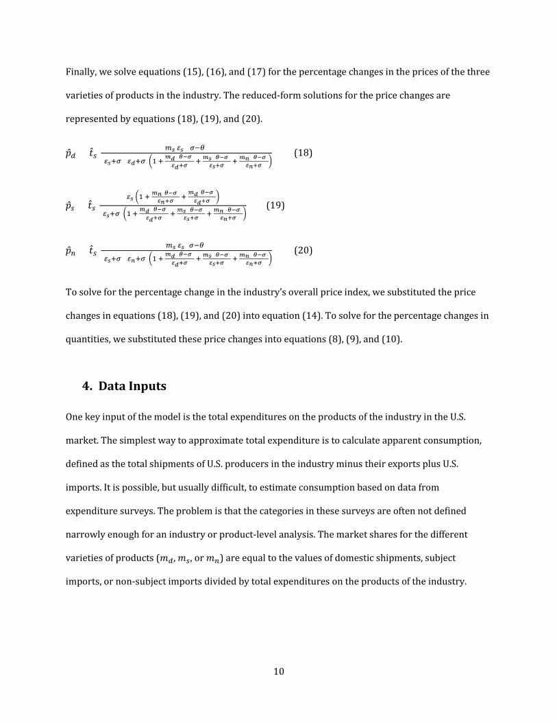
Finally, we solve equations (15), (16), and (17) for the percentage changes in the prices of the three

varieties of products in the industry. The reduced-form solutions for the price changes are

represented by equations (18), (19), and (20).

�̂�𝑝𝑑𝑑 = �̂�𝑡𝑠𝑠 𝑚𝑚𝑠𝑠 𝜀𝜀𝑠𝑠 (𝜎𝜎−𝜃𝜃)

(𝜀𝜀𝑠𝑠+𝜎𝜎)(𝜀𝜀𝑑𝑑+𝜎𝜎)�1 + 𝑚𝑚𝑑𝑑 (𝜃𝜃−𝜎𝜎)𝜀𝜀𝑑𝑑+𝜎𝜎

+ 𝑚𝑚𝑠𝑠 (𝜃𝜃−𝜎𝜎)𝜀𝜀𝑠𝑠+𝜎𝜎

+ 𝑚𝑚𝑛𝑛 (𝜃𝜃−𝜎𝜎)𝜀𝜀𝑛𝑛+𝜎𝜎

� (18)

�̂�𝑝𝑠𝑠 = �̂�𝑡𝑠𝑠 𝜀𝜀𝑠𝑠 �1 + 𝑚𝑚𝑛𝑛(𝜃𝜃−𝜎𝜎)

𝜀𝜀𝑛𝑛+𝜎𝜎 + 𝑚𝑚𝑑𝑑(𝜃𝜃−𝜎𝜎)

𝜀𝜀𝑑𝑑+𝜎𝜎�

(𝜀𝜀𝑠𝑠+𝜎𝜎)�1 + 𝑚𝑚𝑑𝑑 (𝜃𝜃−𝜎𝜎)𝜀𝜀𝑑𝑑+𝜎𝜎



� (19)

�̂�𝑝𝑛𝑛 = �̂�𝑡𝑠𝑠 𝑚𝑚𝑠𝑠 𝜀𝜀𝑠𝑠 (𝜎𝜎−𝜃𝜃)

(𝜀𝜀𝑠𝑠+𝜎𝜎)(𝜀𝜀𝑛𝑛+𝜎𝜎)�1 + 𝑚𝑚𝑑𝑑 (𝜃𝜃−𝜎𝜎)𝜀𝜀𝑑𝑑+𝜎𝜎



� (20)

To solve for the percentage change in the industry’s overall price index, we substituted the price

changes in equations (18), (19), and (20) into equation (14). To solve for the percentage changes in

quantities, we substituted these price changes into equations (8), (9), and (10).

4. Data Inputs

One key input of the model is the total expenditures on the products of the industry in the U.S.

market. The simplest way to approximate total expenditure is to calculate apparent consumption,

defined as the total shipments of U.S. producers in the industry minus their exports plus U.S.

imports. It is possible, but usually difficult, to estimate consumption based on data from

expenditure surveys. The problem is that the categories in these surveys are often not defined

narrowly enough for an industry or product-level analysis. The market shares for the different

varieties of products (𝑚𝑚𝑑𝑑, 𝑚𝑚𝑠𝑠, or 𝑚𝑚𝑛𝑛) are equal to the values of domestic shipments, subject

imports, or non-subject imports divided by total expenditures on the products of the industry.

11

A second key input is the elasticity of substitution among the products, 𝜎𝜎. This parameter value is

often taken from estimates in the academic econometrics literature.7 It may be possible to generate

a new econometric estimate of this model parameter for the model if there are no estimates

available in the literature.8 One way to reflect uncertainty about the value of this parameter is to

report the estimates of economic impacts for a range of potential parameter values rather than a

single value.9

The parameter 𝜃𝜃 is the absolute value of the price elasticity of total demand in the industry. This

model parameter could also be estimated in a new econometric analysis or it could be borrowed

from the literature. The appropriate value of this parameter depends on specific conditions in the

industry. For example, if there were no products from outside of the industry that serve as

substitutes for the products of the industry, then this price elasticity would be very small.

Likewise, the appropriate values for the supply elasticities (𝜀𝜀𝑑𝑑 , 𝜀𝜀𝑠𝑠, and 𝜀𝜀𝑛𝑛) depend on conditions in

the industry. An extreme but useful simplification is to assume that these supply elasticities are

infinite.10 In this case, prices do not change in response to the policy change.

The simulation model is static, rather than dynamic. This means that it does not predict the speed of

adjustment in prices and quantities after the policy change. Still, timing can be roughly

incorporated into the model through the selection of the values of the elasticity parameters – lower

elasticities for an analysis of short-run effects and higher elasticities for a longer-run analysis –

though this is probably a poor substitute for an explicitly dynamic model.

7 For example, Hertel, Hummel, Ivanic, and Keeney (2007) reports estimates of this elasticity at a fairly disaggregated industry level. 8 For example, this is the approach in the analysis of household appliances in Hallren and Riker (2017). 9 Another more elaborate way to reflect the uncertainty in the parameter values is to run Monte Carlo simulations over a distribution of potential values, as in Hallren and Opanasets (2016). 10 For example, Hallren and Opanasets (2016) adopt this assumption for the upstream products in their model.

12

5. Illustrative Application #1: Reductions in Ad Valorem Tariffs

In this section, we report several applications of the model. In our first example, we model a

reduction in the import ad-valorem tariff applied to subject imports from 5 to 0 percent. Figure 2

illustrates the adjustments that result from the tariff change. When the tariff is removed, the supply

of subject imports increases, and the market price of subject imports falls. Because the three

varieties are substitutes, the decline in the market price of subject imports causes consumers to buy

more of the subject imports in lieu of the other two varieties, and this is reflected as a reduction in

demand for the domestic and non-subject varieties. The model predicts that removing a tariff on

subject imports will result in a decline in the market price of all varieties, an increase in quantity

demanded of subject imports, and a decrease in quantity demanded of the domestic product and

non-subject imports.

Table 2 reports the estimated magnitudes of the changes in the prices of the three varieties of

products, the industry’s overall price index, and the quantities of the products as a result of a

reduction in the ad valorem tariff on subject imports from 5 to 0 percent. This implies a 4.76

US Subject Non-subject

D

S

A

ln pd

ln qd ln qs

ln qn

D

S + T

D

S

S

D’ D’

B

A

B

A

B

Figure 2: Eliminating the import tariff

ln ps ln pn

13

percent reduction in 𝑡𝑡𝑠𝑠 (if there are no international transport costs in 𝑡𝑡𝑠𝑠). The table reports five

different versions of the model with alternative assumptions about market shares and elasticity

parameters.

14

Table 2: Reducing an Ad Valorem Tariff

v1 v2 v3 v4 v5

Data Inputs

Market Share of Domestic Producers (percent) 33.33 70.00 33.33 33.33 33.33

Market Share of Subject Imports (percent) 33.33 10.00 33.33 33.33 33.33

Market Share of Non-Subject Imports (percent) 33.33 20.00 33.33 33.33 33.33

Supply Elasticity for Domestic Producers 1 1 5 1 1

Supply Elasticity for Subject Imports 10 10 10 10 10

Supply Elasticity for Non-Subject Imports 10 10 10 10 10

Elasticity of Substitution within the Industry 5 5 5 5 6

Price Elasticity of Total Industry Demand 1 1 1 0.5 1

Changes in Trade Policy

Initial Tariff Rate on Subject Imports (percent) 5.00 5.00 5.00 5.00 5.00

Revised Tariff Rate on Subject Imports (percent) 0.00 0.00 0.00 0.00 0.00

Percentage Changes in Prices

Change in the Price of the Domestic Product -1.18 -0.47 -0.61 -1.44 -1.28

Change in the Price of Subject Imports -3.64 -3.36 -3.58 -3.75 -3.54

Change in the Price of Non-Subject Imports -0.47 -0.19 -0.41 -0.58 -0.56

Change in the Industry Price Index -1.76 -0.70 -1.54 -1.92 -1.79

Percentage Changes in Quantities

Change in the Quantity of the Domestic Product -1.18 -0.47 -3.07 -1.44 -1.28

Change in the Quantity of Subject Imports 11.17 14.01 11.78 10.10 12.26

Change in the Quantity of Non-Subject Imports -4.70 -1.87 -4.10 -5.77 -5.60

In the first version of the model (column v1 in table 2), the tariff change reduces the price of subject

imports by 3.64 percent and reduces the prices of the domestic product and non-subject imports by

1.18 and 0.47 percent. The industry’s overall price index falls 1.76 percent. The reduction in the

tariff on subject imports increases the quantity of subject imports by 11.17 percent but reduces the

quantity of domestic product and non-subject imports by 1.18 and 4.70 percent.

15

The remaining columns in the table report the sensitivity of these estimates to the data inputs of

the model. Alternative v2 shows that, all else equal, a larger market share of domestic producers

and a smaller market share of subject imports reduces the absolute magnitudes of all of the price

and quantity changes except the increase in the quantity of subject imports, which is magnified.11

Alternative v3 shows that greater supply elasticity of domestic producers (relative to the

benchmark value in alternative v1) reduces the magnitude of the decline in the price of domestic

producers but increases the decline in their quantity. Alternative v4 shows that a reduction in the

price elasticity of total industry demand increases the decline in all of the prices and increases the

decline in the quantity of the domestic product. Finally, alternative v5 shows that an increase in the

elasticity of substitution (relative to the benchmark value) increases the percentage declines in

prices of domestic products and non-subject imports and also increases the percentage declines in

the quantities of these products.

6. Illustrative Application #2: Increase in an Import Quota

In our second example, we model an increase in a binding import quota. By binding we mean that

equilibrium, consumers will purchase the full amount of subject imports allowed under the quota.

Figure 3 illustrates the adjustments resulting from this policy change. The supply curve for subject

imports is the line 𝑎𝑎𝑏𝑏𝑎𝑎𝑎𝑎�� without any quota. With the initial quota in place, the supply curve is line

𝑎𝑎𝑏𝑏𝑎𝑎𝑎𝑎��. Buyers can purchase up to the quota amount. At that amount, the supply curve becomes

perfectly inelastic and any increase in demand translates into an increase in the market price for

subject imports with no further changes in quantity. When the quota is increased, the supply curve

for subject imports becomes 𝑎𝑎𝑏𝑏𝑎𝑎𝑎𝑎′��.

11 A smaller tariff reduction would also reduce the absolute magnitudes of all of the quantity and price changes.

16

US Subject Non-subject

D

S

A

D

S’

D

S S

D’ D’

B

A B

A B

a

b

c

Figure 3: Increasing the import quota

Given the demand for subject imports, the market price of subject imports falls. Because the three

varieties (domestic, subject, and non-subject) are substitutes, when the price of subject imports

falls, demand for the other two varieties declines. Consequently, the effects of increasing a binding

import quota are a reduction in the market price of all varieties, an increase in the market share of

subject imports, and a decline in the market shares of domestic and non-subject imports.

The derivation of the equations of the model in section 2 focuses on a change in an ad valorem

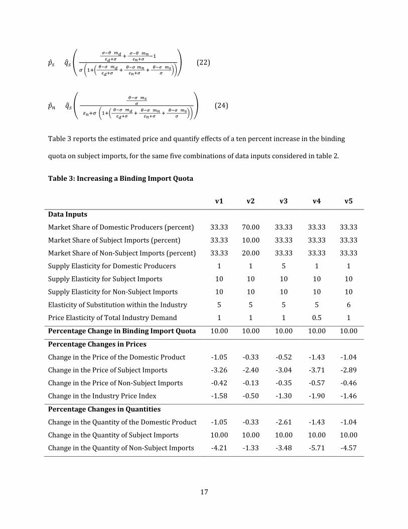
tariff. We can also derive the equations for a change in the binding quota. In this case, 𝑞𝑞�𝑠𝑠 is an

exogenous parameter in equation (12), and equation (9) drops from the model.12 Equations (21),

(22), and (23) quantify the resulting percentage changes in the prices of the three varieties, and

equation (14) still defines the percentage change in the industry’s overall price index.

�̂�𝑝𝑑𝑑 = 𝑞𝑞�𝑠𝑠 � (𝜃𝜃−𝜎𝜎) 𝑚𝑚𝑠𝑠

𝜎𝜎

(𝜀𝜀𝑑𝑑+𝜎𝜎)�1+�(𝜃𝜃−𝜎𝜎) 𝑚𝑚𝑑𝑑𝜀𝜀𝑑𝑑+𝜎𝜎

+ (𝜃𝜃−𝜎𝜎) 𝑚𝑚𝑛𝑛𝜀𝜀𝑛𝑛+𝜎𝜎

+ (𝜃𝜃−𝜎𝜎) 𝑚𝑚𝑠𝑠𝜎𝜎 ��

� (21)

12 Exogeneity means that the quantity imported is not determined by market prices. It is set by trade policy.

ln pd ln ps

ln pn

ln qn

ln qs

ln qd

17

�̂�𝑝𝑠𝑠 = 𝑞𝑞�𝑠𝑠 � (𝜎𝜎−𝜃𝜃) 𝑚𝑚𝑑𝑑𝜀𝜀𝑑𝑑+𝜎𝜎

+ (𝜎𝜎−𝜃𝜃) 𝑚𝑚𝑛𝑛𝜀𝜀𝑛𝑛+𝜎𝜎

−1

𝜎𝜎 �1+�(𝜃𝜃−𝜎𝜎) 𝑚𝑚𝑑𝑑𝜀𝜀𝑑𝑑+𝜎𝜎

+ (𝜃𝜃−𝜎𝜎)𝑚𝑚𝑛𝑛𝜀𝜀𝑛𝑛+𝜎𝜎


� (22)

�̂�𝑝𝑛𝑛 = 𝑞𝑞�𝑠𝑠 � (𝜃𝜃−𝜎𝜎) 𝑚𝑚𝑠𝑠

𝜎𝜎

(𝜀𝜀𝑛𝑛+𝜎𝜎)�1+�(𝜃𝜃−𝜎𝜎) 𝑚𝑚𝑑𝑑𝜀𝜀𝑑𝑑+𝜎𝜎

+ (𝜃𝜃−𝜎𝜎) 𝑚𝑚𝑛𝑛𝜀𝜀𝑛𝑛+𝜎𝜎


� (24)

Table 3 reports the estimated price and quantify effects of a ten percent increase in the binding

quota on subject imports, for the same five combinations of data inputs considered in table 2.

Table 3: Increasing a Binding Import Quota

v1 v2 v3 v4 v5

Data Inputs








Price Elasticity of Total Industry Demand 1 1 1 0.5 1

Percentage Change in Binding Import Quota 10.00 10.00 10.00 10.00 10.00










18

Like the reduction in a tariff on subject imports, the increase in a binding quota on subject imports

reduces the price of subject imports and reduces the prices of the domestic product and non-

subject imports (column v1 in table 2). The increase in the quota increases the quantity of subject

imports and reduces the quantity of domestic product and non-subject imports.

Again, the remaining columns of the table report the sensitivity of the magnitude of the percentage

changes to the data inputs. Alternative v2 shows that, all else equal, a larger market share of

domestic producers and a smaller market share of subject imports reduces the absolute

magnitudes of all of the quantity and price changes (except the percentage change in the quantity of

subject imports, which is set by the increase in the quota). Alternative v3 shows that greater supply

elasticity of domestic producers (relative to the benchmark value in alternative v1) reduces the

magnitude of the decline in the price of domestic producers but increases the decline in their

quantity of their domestic shipments. Alternative v4 shows that a reduction in the price elasticity of

total industry demand increases the decline in all of the prices and increases the decline in the

quantity of the domestic product. Finally, alternative v5 shows that an increase in the elasticity of

substitution (relative to the benchmark value) reduces the declines in the price and quantity of

domestic products.

19

7. Non-Linear Versions of the Models

We reran the simulations using the exact non-linear functional forms in equations (1) through (7),

which are log-linear, as well as the CES price index for the industry, which is not log-linear.

To solve the non-linear version of the model, one uses an iterative algorithm to find the set of prices

that ensures that quantity supplied equals quantity demanded in all markets simultaneously. Fetzer

(2005) describes the derivation of the following set of equations.

�𝑝𝑝𝑖𝑖𝑡𝑡𝑖𝑖�𝜀𝜀𝑖𝑖

= 𝑃𝑃𝜎𝜎−𝜃𝜃

𝑝𝑝𝑖𝑖𝜎𝜎 𝑓𝑓𝑓𝑓𝑓𝑓 𝑎𝑎𝑎𝑎𝑎𝑎 𝑖𝑖 ∈ 𝑑𝑑𝑓𝑓𝑚𝑚, 𝑠𝑠𝑠𝑠𝑏𝑏𝑠𝑠,𝑛𝑛𝑓𝑓𝑛𝑛 − 𝑠𝑠𝑠𝑠𝑏𝑏𝑠𝑠

We solve the model in Excel by via an iterative algorithm that solves the following sum of squared

errors (SSE) minimization problem:

min𝑝𝑝𝑖𝑖

𝑎𝑎𝑎𝑎𝑆𝑆 = min𝑝𝑝𝑖𝑖

��𝑝𝑝𝑖𝑖𝑡𝑡𝑖𝑖�𝜀𝜀𝑖𝑖− 𝑃𝑃𝜎𝜎−𝜃𝜃

𝑝𝑝𝑖𝑖𝜎𝜎�2

Table 4 is a side-by-side comparison the simulation results for the first two versions of the

reduction in an ad valorem tariff, using the log-linearized model as in Table 2 and then using the

exact non-linear model. The estimated price and quantity effects are amplified (the percentage

changes are larger in absolute value) using the non-linear model, but the differences are small,

reflecting the fact that the model is almost completely log-linear before any linearization.

20

Table 4: Comparison of Models for a Reduction in an Ad Valorem Tariff

Log-

Linearized

v1

Non-

Linear

v1

Log-

Linearized

v2

Non-

Linear

v2

Data Inputs

Market Share of Domestic Producers (percent) 33.33 33.33 70.00 70.00

Market Share of Subject Imports (percent) 33.33 33.33 10.00 10.00

Market Share of Non-Subject Imports (percent) 33.33 33.33 20.00 20.00

Supply Elasticity for Domestic Producers 1 1 1 1

Supply Elasticity for Subject Imports 10 10 10 10

Supply Elasticity for Non-Subject Imports 10 10 10 10

Elasticity of Substitution within the Industry 5 5 5 5

Price Elasticity of Total Industry Demand 1 1 1 1


Initial Tariff Rate on Subject Imports (percent) 5.00 5.00 5.00 5.00

Revised Tariff Rate on Subject Imports (percent) 0.00 0.00 0.00 0.00


Change in the Price of the Domestic Product -1.18 -1.24 -0.47 -0.50

Change in the Price of Subject Imports -3.64 -3.68 -3.36 -3.40

Change in the Price of Non-Subject Imports -0.47 -0.50 -0.19 -0.20

Change in the Industry Price Index -1.76 -1.85 -0.70 -0.75


Change in the Quantity of the Domestic Product -1.18 -1.24 -0.47 -0.50

Change in the Quantity of Subject Imports 11.17 11.35 14.01 14.35

Change in the Quantity of Non-Subject Imports -4.70 -4.97 -1.87 -2.01

Table 5 is a side-by-side comparison the simulation results for the first two versions of the increase

in a binding quota, using the log-linearized model as in Table 3 and then using the exact non-linear

model. The estimated price and quantity effects are dampened (the percentage changes are smaller

in absolute value) using the non-linear model, but the differences are very small.

21

Table 5: Comparison of Models for an Increase in a Binding Import Quota

Log-

Linear

v1

Non-

Linear

v1

Log-

Linear

v2

Non-

Linear

v2

Data Inputs

Market Share of Domestic Producers (percent) 33.33 33.33 70.00 70.00

Market Share of Subject Imports (percent) 33.33 33.33 10.00 10.00

Market Share of Non-Subject Imports (percent) 33.33 33.33 20.00 20.00

Supply Elasticity for Domestic Producers 1 1 1 1

Supply Elasticity for Subject Imports 10 10 10 10

Supply Elasticity for Non-Subject Imports 10 10 10 10

Elasticity of Substitution within the Industry 5 5 5 5

Price Elasticity of Total Industry Demand -1 -1 -1 -1

Percentage Change in Binding Import Quota 10.00 10.00 10.00 10.00


Change in the Price of the Domestic Product -1.05 -1.04 -0.33 -0.33

Change in the Price of Subject Imports -3.26 -3.11 -2.40 -2.28

Change in the Price of Non-Subject Imports -0.42 -0.42 -0.13 -0.13

Change in the Industry Price Index -1.58 -1.55 -0.50 -0.49


Change in the Quantity of the Domestic Product -1.05 -1.04 -0.33 -0.33

Change in the Quantity of Subject Imports 10.00 10.00 10.00 10.00

Change in the Quantity of Non-Subject Imports -4.21 -4.16 -1.33 -1.32

These examples suggest that it does not really matter whether the effects are calculated using a log-

linearized model or the exact non-linear model. The log-linearized model is easier to implement, as

simple cell formulas in Excel, but the non-linear model is also pretty straightforward to implement

using a non-linear solver.

22

8. Conclusion

As we noted in the Introduction, there are many advantages to using a simpler modeling framework

when analyzing the effects of trade policy changes that are narrowly targeting a specific industry.

The model can provide quantitative estimates based on limited data inputs. It is easy to create,

modify, and run.13 The model is calibrated to the details the industry. For these reasons, industry-

specific models can be very useful as a first cut analysis, prior to more detailed economic modeling,

or as a test kitchen for experimentally adding new complexities into trade policy analysis.

The basic partial equilibrium model can be extended in many directions to better fit the economic

complexities of the industry analyzed.14 For example, the beef model in Hallren and Opanasets

(2016) includes vertically integrated production and trade in intermediate products. The household

appliances model in Hallren and Riker (2017) includes sub-national regions within the United

States. The models of architectural, engineering, and legal services in Khachaturian and Riker

(2016, 2017) and Barbe, Chambers, Khachaturian and Riker (2017) include multiple modes of

international supply of the services (e.g., cross-border exports and foreign affiliate sales) and fixed

costs of trade, as well as ad valorem tariffs. The equations and data requirements of these extended

models are more elaborate, but the principles of model building are the same.

13 The model used in the illustrative applications in tables 2 and 3 is run in an Excel worksheet with simple cell formulas. 14 The following examples are USITC research papers that are available at https://www.usitc.gov/research_and_analysis/staff_products.htm.

23

References Armington, Paul S. (1969): “A Theory of Demand for Products Distinguished by Place of Production.” Staff Papers (International Monetary Fund) 16 (1): 159-78.

Barbe, Andre, Arthur Chambers, Tamar Khachaturian and David Riker (2017): “Modeling Trade in Services: Multiple Modes, Barriers to Trade, and Data Limitations.” USITC Economics Working Paper No. 2017-04-B.

Fetzer, James J. (2005): “A Partial Equilibrium Approach of Modeling Vertical Linkages in the U.S. Flat Rolled Steel Market.” USITC Economics Working Paper No. 2005-01-A.

Hallren, Ross and Alexandra Opanasets (2016): “Whence the Beef? The Effects of Repealing Mandatory Country of Origin Labeling (COOL) using a Vertically Integrated Armington Model with Monte Carlo Simulation.” USITC Economics Working Paper No. 2016-09-A.

Hallren, Ross and David Riker (2017): “A U.S. Regional Model of Import Competition and Jobs.” USITC Economics Working Paper No. 2017-2-A.

Hertel, Thomas, David Hummel, Maros Ivanic, and Roman Keeney (2007): “How Confident Can We Be of CGE-Based Assessments of Free Trade Agreements.” Economic Modeling 24 (4): 611-635.

Khachaturian, Tamar and David Riker (2016): “A Multi-Mode Partial Equilibrium Model of Trade in Professional Services.” USITC Economics Working Paper No. 2016-10-A.

Khachaturian, Tamar and David Riker (2017): “The Impact of Liberalizing International Trade in Professional Services.” Journal of International Commerce and Economics, May 2017.

24

Appendix: Simulations Using a Non-Linear Version of the Models

Table A1: Non-Linear Model of a Reduction in an Ad Valorem Tariffs

v1 v2 v3 v4 v5

Data Inputs








Price Elasticity of Total Industry Demand -1 -1 -1 -0.5 -1


Initial Tariff Rate on Subject Imports (percent) 5.00 5.00 5.00 5.00 5.00

Revised Tariff Rate on Subject Imports (percent) 0.00 0.00 0.00 0.00 0.00










25

Table A2: Non-Linear Model of an Increase in a Binding Import Quota

v1 v2 v3 v4 v5

Data Inputs








Price Elasticity of Total Industry Demand -1 -1 -1 -0.5 -1

Percentage Change in Binding Import Quota 10.00 10.00 10.00 10.00 10.00










An Introduction to Partial Equilibrium Modeling of Trade ... · AN INTRODUCTION TO PARTIAL...

Documents

Transcript of An Introduction to Partial Equilibrium Modeling of Trade ... · AN INTRODUCTION TO PARTIAL...