
An Introduction to Nonlinear Waves - … · The aim of these notes is to give an introduction to...
163
An Introduction to Nonlinear Waves Erik Wahlén
Transcript of An Introduction to Nonlinear Waves - … · The aim of these notes is to give an introduction to...
An Introduction to Nonlinear Waves
Erik Wahlén

Copyright c© 2011 Erik Wahlén

Preface
The aim of these notes is to give an introduction to the mathematics of nonlinear waves.The waves are modelled by partial differential equations (PDE), in particular hyperbolic ordispersive equations. Some aspects of completely integrable systems and soliton theory arealso discussed. While the goal is to discuss the nonlinear theory, this cannot be achievedwithout first discussing linear PDE. The prerequisites include a good background in real andcomplex analysis, vector calculus and ordinary differential equations. Some basic knowledgeof Lebesgue integration and (the language of) functional analysis is also useful. There are twoappendices providing the necessary background in these areas. I have not assumed any priorknowledge of PDE.
The notes have been used for a graduate course on nonlinear waves in Lund, 2011. Iwant to thank my students Fatemeh Mohammadi, Karl-Mikael Perfekt and Johan Richter forpointing out some errors. I also want to thank my colleague Mats Ehrnstöm for letting me useparts of his lecture notes on ‘Waves and solitons’.
Erik Wahlén,Lund, December 2011
3


Contents
Preface . . . . . . . . . . . . . . . . . . . . . . . . . . . . . . . . . . . . . 3
1 Introduction 91.1 Linear waves . . . . . . . . . . . . . . . . . . . . . . . . . . . . . . . . . . 9
1.1.1 Sinusoidal waves . . . . . . . . . . . . . . . . . . . . . . . . . . . . 91.1.2 The wave equation . . . . . . . . . . . . . . . . . . . . . . . . . . . 101.1.3 Dispersion . . . . . . . . . . . . . . . . . . . . . . . . . . . . . . . 14
1.2 Nonlinear waves . . . . . . . . . . . . . . . . . . . . . . . . . . . . . . . . 161.3 Solitons . . . . . . . . . . . . . . . . . . . . . . . . . . . . . . . . . . . . . 18
2 The Fourier transform 252.1 The Schwartz space . . . . . . . . . . . . . . . . . . . . . . . . . . . . . . . 252.2 The Fourier transform on S . . . . . . . . . . . . . . . . . . . . . . . . . . 272.3 Extension of the Fourier transform to Lp . . . . . . . . . . . . . . . . . . . . 31
3 Linear PDE with constant coefficients 353.1 The heat equation . . . . . . . . . . . . . . . . . . . . . . . . . . . . . . . . 36
3.1.1 Derivation . . . . . . . . . . . . . . . . . . . . . . . . . . . . . . . . 363.1.2 Solution by Fourier’s method . . . . . . . . . . . . . . . . . . . . . . 373.1.3 The heat kernel . . . . . . . . . . . . . . . . . . . . . . . . . . . . . 403.1.4 Qualitative properties . . . . . . . . . . . . . . . . . . . . . . . . . . 41
3.2 The wave equation . . . . . . . . . . . . . . . . . . . . . . . . . . . . . . . 433.2.1 Derivation . . . . . . . . . . . . . . . . . . . . . . . . . . . . . . . . 433.2.2 Solution by Fourier’s method . . . . . . . . . . . . . . . . . . . . . . 443.2.3 Solution formulas . . . . . . . . . . . . . . . . . . . . . . . . . . . . 443.2.4 Qualitative properties . . . . . . . . . . . . . . . . . . . . . . . . . . 48
3.3 The Laplace equation . . . . . . . . . . . . . . . . . . . . . . . . . . . . . . 513.4 General PDE and the classification of second order equations . . . . . . . . . 523.5 Well-posedness of the Cauchy problem . . . . . . . . . . . . . . . . . . . . . 543.6 Hyperbolic operators . . . . . . . . . . . . . . . . . . . . . . . . . . . . . . 61
4 First order quasilinear equations 654.1 Some definitions . . . . . . . . . . . . . . . . . . . . . . . . . . . . . . . . 654.2 The method of characteristics . . . . . . . . . . . . . . . . . . . . . . . . . . 674.3 Conservation laws . . . . . . . . . . . . . . . . . . . . . . . . . . . . . . . . 69
5

6
4.3.1 Discontinuous solutions . . . . . . . . . . . . . . . . . . . . . . . . 754.3.2 The Riemann problem . . . . . . . . . . . . . . . . . . . . . . . . . 774.3.3 Entropy conditions . . . . . . . . . . . . . . . . . . . . . . . . . . . 79
5 Distributions and Sobolev spaces 835.1 Distributions . . . . . . . . . . . . . . . . . . . . . . . . . . . . . . . . . . 845.2 Operations on distributions . . . . . . . . . . . . . . . . . . . . . . . . . . . 855.3 Tempered distributions . . . . . . . . . . . . . . . . . . . . . . . . . . . . . 875.4 Approximation with smooth functions . . . . . . . . . . . . . . . . . . . . . 915.5 Sobolev spaces . . . . . . . . . . . . . . . . . . . . . . . . . . . . . . . . . 92
6 Dispersive equations 976.1 Calculus in Banach spaces . . . . . . . . . . . . . . . . . . . . . . . . . . . 986.2 NLS . . . . . . . . . . . . . . . . . . . . . . . . . . . . . . . . . . . . . . . 101
6.2.1 Linear theory . . . . . . . . . . . . . . . . . . . . . . . . . . . . . . 1016.2.2 Nonlinear theory . . . . . . . . . . . . . . . . . . . . . . . . . . . . 105
6.3 KdV . . . . . . . . . . . . . . . . . . . . . . . . . . . . . . . . . . . . . . . 1126.3.1 Linear theory . . . . . . . . . . . . . . . . . . . . . . . . . . . . . . 1126.3.2 Nonlinear theory . . . . . . . . . . . . . . . . . . . . . . . . . . . . 1156.3.3 Derivation of the KdV equation . . . . . . . . . . . . . . . . . . . . 123
6.4 Further reading . . . . . . . . . . . . . . . . . . . . . . . . . . . . . . . . . 125
7 Solitons and complete integrability 1277.1 Miura’s transformation, Gardner’s extension and infinitely many conservation
laws . . . . . . . . . . . . . . . . . . . . . . . . . . . . . . . . . . . . . . . 1287.2 Soliton solutions . . . . . . . . . . . . . . . . . . . . . . . . . . . . . . . . 1297.3 Lax pairs . . . . . . . . . . . . . . . . . . . . . . . . . . . . . . . . . . . . 134
7.3.1 The scattering problem . . . . . . . . . . . . . . . . . . . . . . . . . 1347.3.2 The evolution equation . . . . . . . . . . . . . . . . . . . . . . . . . 1357.3.3 The relation to Lax pairs . . . . . . . . . . . . . . . . . . . . . . . . 1377.3.4 A Lax-pair formulation for the KdV equation . . . . . . . . . . . . . 139
A Functional analysis 141A.1 Banach spaces . . . . . . . . . . . . . . . . . . . . . . . . . . . . . . . . . . 141A.2 Hilbert spaces . . . . . . . . . . . . . . . . . . . . . . . . . . . . . . . . . . 144A.3 Metric spaces and Banach’s fixed point theorem . . . . . . . . . . . . . . . . 145A.4 Completions . . . . . . . . . . . . . . . . . . . . . . . . . . . . . . . . . . . 146
B Integration 149B.1 Lebesgue measure . . . . . . . . . . . . . . . . . . . . . . . . . . . . . . . . 149B.2 Lebesgue integral . . . . . . . . . . . . . . . . . . . . . . . . . . . . . . . . 151B.3 Convergence properties . . . . . . . . . . . . . . . . . . . . . . . . . . . . . 153B.4 Lp spaces . . . . . . . . . . . . . . . . . . . . . . . . . . . . . . . . . . . . 154B.5 Convolutions and approximation with smooth functions . . . . . . . . . . . . 156

7
B.6 Interpolation . . . . . . . . . . . . . . . . . . . . . . . . . . . . . . . . . . . 159

8

Chapter 1
Introduction
You are probably familiar with many different kinds of wave phenomena such as surfacewaves on the ocean, sound waves in the air or other media, and electromagnetic waves, ofwhich visible light is a special case. A common feature of these examples is that they all canbe described by partial differential equations (PDE). The purpose of these lecture notes is togive an introduction to various kinds of PDE describing waves. In particular we will focus onnonlinear equations. In this chapter we introduce some basic concepts and give an overviewof the contents of the lecture notes.
1.1 Linear waves
1.1.1 Sinusoidal wavesThe first encounter with the mathematical theory of waves is usually with cosine (or sine)waves of the form
u(x, t) = acos(kx±ωt).
Here x, t ∈ R denote space and time, respectively, and the parameters a, k and ω are positivenumbers. a is the amplitude of the wave, k the wave number and ω the angular frequency.Note that u is periodic in both space and time with periods
λ =2π
k
andT =
2π
ω.
λ is usually called the wavelength and T simply the period. The wave has crests (local max-ima) when kx±ωt is an even multiple of π and troughs (local minima) when it is an oddmultiple of π .
Rewriting u asu(x, t) = acos(k(x± ct)),
9

10 Introduction
c
xa
Figure 1.1: A cosine wave.
wherec =
ω
k, (1.1)
we see that as t changes, the fixed shape
X 7→ cos(kX)
is simply being translated at constant speed c along the x-axis. The number c is called the wavespeed or phase speed. The wave moves to the left if the sign is positive and to the right if thesign is negative. A wave of permanent shape moving at constant speed is called a travellingwave or sometimes a steady wave.
1.1.2 The wave equation
Assume that the phenomenon being studied is linear so that more complicated wave forms canbe obtained by adding different cosine waves. In order to do this, we must be more specificabout the relation between the parameters c and k (the parameter ω is determined by c and kthrough (1.1)). One often makes the assumption that c is independent of k, so that all cosinewaves move at the same speed. Note that the waves then satisfy the PDE
utt(x, t) = c2uxx(x, t) (1.2)
(subscripts denote partial derivatives). This is the wave equation in one (spatial) dimension.The assumption that one can add the waves together agrees with the linearity of the waveequation; any linear combination of solutions of (1.2) is also a solution of (1.2).
A better way of deriving the wave equation is to start from physical principles. Here is anexample.
Example 1.1. What we perceive as sound is really a pressure wave in the air. Sound wavesare longitudinal waves, meaning that the oscillations take place in the same direction as thewave is moving. The equations governing acoustic waves are the equations of gas dynamics.

Introduction 11
These form a system of nonlinear PDE for the velocity u and the density ρ . Assuming that theoscillations are small, one can derive a set of linearized equations:
ρ0ut + c20∇ρ = 0,
ρt +ρ0∇ ·u = 0,
where ρ0 is the density and c0 the speed of sound in still air. Here u(·, t) : Ω→ R3 whileρ(·, t) : Ω→ R for some open set Ω⊂ R3. If we consider a one-dimensional situation (e.g. athin pipe), the system simplifies to
ρ0ut + c20ρx = 0,
ρt +ρ0ux = 0.
Differentiating both equations with respect to t and x, we obtain after some simplificationsthat both u and ρ satisfy the wave equation:
utt = c20uxx
and
ρtt = c20ρxx.
Note that ρ describes the fluctuation of the density around ρ0. In the linear approximation,the pressure fluctuation p around the constant atmospheric pressure is simply proportional toρ . It follows that p also satisfies the wave equation. The nonlinear equations of gas dynamicswill be discussed in Chapter 4.
We have assumed that the waves are even in x± ct. To find the most general form of thewave we also have to include terms of the form sin(k(x± ct)). In order to make the notationsimpler it is convenient to use the complex exponential function. The original real-valuedfunction can be recovered by separating into real and imaginary parts. It is convenient also toallow k to be negative. A general linear combination of sinusoidal waves can be written
u(x, t) = ∑k(akeik(x−ct)+bkeik(x+ct)),
which is often rewritten (with other coefficients) in the form
u(x, t) = ∑k
eikx(ak cos(kct)+bk sin(kct)).
Depending on the physical situation there might be boundary conditions which limit the rangeof wave numbers k. We might e.g. only look for a wave in a bounded interval, say [0,π], whichvanishes at the end points. This forces us to look for solutions of the form
u(x, t) =∞
∑k=1
sin(kx)(ak cos(kct)+bk sin(kct)).

12 Introduction
In these notes we will not discuss boundaries, and hence there is no restriction on k. The mostgeneral linear combination is then not a sum, but an integral
u(x, t) =∫R
eiξ x(a(ξ )cos(ξ ct)+b(ξ )sin(ξ ct))dξ
(we have changed k to ξ to emphasize that it is a continuous variable). If you have studiedFourier analysis, you will recognize this as a Fourier integral. Suppose that we know theinitial position and velocity of u, that is, u(x,0) and ut(x,0). Then a and b are determined by
u(x,0) =∫R
eiξ xa(ξ )dξ
andut(x,0) =
∫R
eiξ xcξ b(ξ )dξ .
There are of course many question marks to be sorted out if one wants to make this intorigorous mathematics. In particular, one has to know that the functions u(x,0) and ut(x,0)can be written as Fourier integrals and that the functions a and b are unique. This question isdiscussed in Chapters 2 and 6. In Chapter 3 we will discuss the application of Fourier methodsto solving PDE such as the wave equation.
There is also another way of solving the wave equation discovered by d’Alembert. Theidea is that the equation can be rewritten in the factorized form
(∂t− c∂x)(∂t + c∂x)u = 0.
Introducing the new variable v = ut + cux, we therefore obtain the two equations
ut + cux = v,vt− cvx = 0.
The expression vt − cvx is the directional derivative of the function v in the direction (−c,1).The second equation therefore expresses that v is constant on the lines x+ct = const. In otherwords, v is a function of x+ ct, v(x, t) = f (x+ ct). The first equation now becomes
ut + cux = f (x+ ct)
The left hand side of this equation can be interpreted as the directional derivative of u inthe direction (c,1). Evaluating u along the straight line γ(s) = (y+ cs,s), where y ∈ R is aparameter, we find that
dds((u γ)(s)) = (v γ)(s),
and hence
(u γ)(s) =∫(v γ)(r)dr
=∫
f (y+2cr)dr
= F(y+2cs)+G(y)

Introduction 13
where F(s) = 12c∫ s
0 f (r)dr and G(y) is an integration constant (∫
is used to denote the indefi-nite integral). Setting s = t, y = x− ct, we obtain that
u(x, t) = F(x+ ct)+G(x− ct).
This can interpreted as saying that the general solution is a sum of a wave moving to the left,F(x+ ct), and a wave moving to the right, G(x− ct). One usually derives this formula bymaking the change of variables y = x− ct, z = x+ ct, which results in the equation uyz = 0.The approach used here is however useful to keep in mind when we discuss the method ofcharacteristics in Chapter 4 (see also Section 1.2 below).
The functions F and G can again be uniquely determined once we know the initial datau(x,0) = u0(x) and ut(x,0) = u1(x). Indeed, we obtain the system of equations
F +G = u0,
F−G =1c
U1,
where U ′1 = u1, which has the unique solution
F =12
u0 +12c
U1,
G =12
u0−12c
U1
Since U1(s) =∫ s
0 u1(r)dr+C, this results in d’Alembert’s solution formula
u(x, t) =12(u0(x+ ct)+u0(x− ct))+
12c
∫ x+ct
x−ctu1(s)ds.
Since we have derived a formula for the solution, it follows that it is unique under suitableregularity assumptions.
Theorem 1.2. Assume that u0 ∈C2(R), u1 ∈C1(R) and c > 0. There exists a unique solutionu ∈C2(R2) of the initial-value problem
utt = c2uxx
u(x,0) = u0(x)ut(x,0) = u1(x).
The solution is given by d’Alembert’s formula
u(x, t) =12(u0(x+ ct)+u0(x− ct))+
12c
∫ x+ct
x−ctu1(s)ds.

14 Introduction
1.1.3 DispersionIn many cases, the assumption that c is constant as a function of k is unrealistic. If c is anon-constant function of k one says that the wave (or rather the equation) is dispersive. Thismeans that waves of different wavelengths travel with different speeds. An initially localizedwave will disintegrate into separate components according to wavelength and disperse. Therelation between ω and k is called the dispersion relation (although some authors use this termfor the relation between c and k).
Example 1.3. The equation
ihut +h2
2muxx = 0
is the one-dimensional version of the famous free Schrödinger equation from quantum me-chanics, describing a quantum system consisting of one particle. h is the reduced Planck’sconstant, and m the mass of the particle. The function u, called the wave function, is complex-valued and its modulus square, |u|2, can be interpreted as a probability density. Assuming thatu is square-integrable and has been normalized so that∫
R|u(x, t)|2 dx = 1,
the probability of finding the particle in the interval [a,b] is given by∫ b
a|u(x, t)|2 dx.
After rescaling t we can rewrite the Schrödinger equation in the form
iut +uxx = 0.
Making the Ansatz u(x, t) = ei(kx−ω(k)t), we obtain the equation
ω(k) = k2
and therefore
c(k) =ω(k)
k= k.
Note that we allow c, k and ω to be negative now, so that waves can travel either to the left(k < 0) or to the right (k > 0).
Example 1.4. The linearized Korteweg-de Vries (KdV) equation
ut +uxxx = 0
appears as a model for small-amplitude water waves with long wavelength. The equationis sometimes called Airy’s equation, although that name is also used for the closely relatedordinary differential equation y′′− xy = 0. Substituting u(x, t) = ei(kx−ω(k)t) into the equation,we find that
ω(k) =−k3
Introduction 15
and hencec(k) =−k2.
The fact that c is negative means that the waves travel to the left.
Since c(k) depends on k for dispersive waves, the wave speed only gives the speed of awave with a single wave number. A different speed can be found if one looks for a solutionwhich consists of a narrow band of wave numbers. For simplicity, we suppose that the equationhas cosine solutions cos(kx−ω(k)t) and consider the sum of two such waves with nearly thesame wave numbers k1 and k2. Let ω1 and ω2 be the corresponding angular frequenciesand suppose that the waves have the same amplitude a. Using the trigonometric identitycos(α)+ cos(β ) = 2cos((α−β )/2)cos((α +β )/2), the sum can be written
2acos((k1− k2)x
2− (ω1−ω2)t
2
)cos((k1 + k2)x
2− (ω1 +ω2)t
2
).
This is a product of two cosine waves, one with wave speed (ω1+ω2)/(k1+k2) and the otherwith speed (ω1−ω2)/(k1− k2). Setting k1 = k0 +∆k and k2 = k0−∆k, we obtain as ∆k→ 0the approximate form
2acos(∆k(x−ω′(k0)t))cos(k0(x− c(k0)t)).
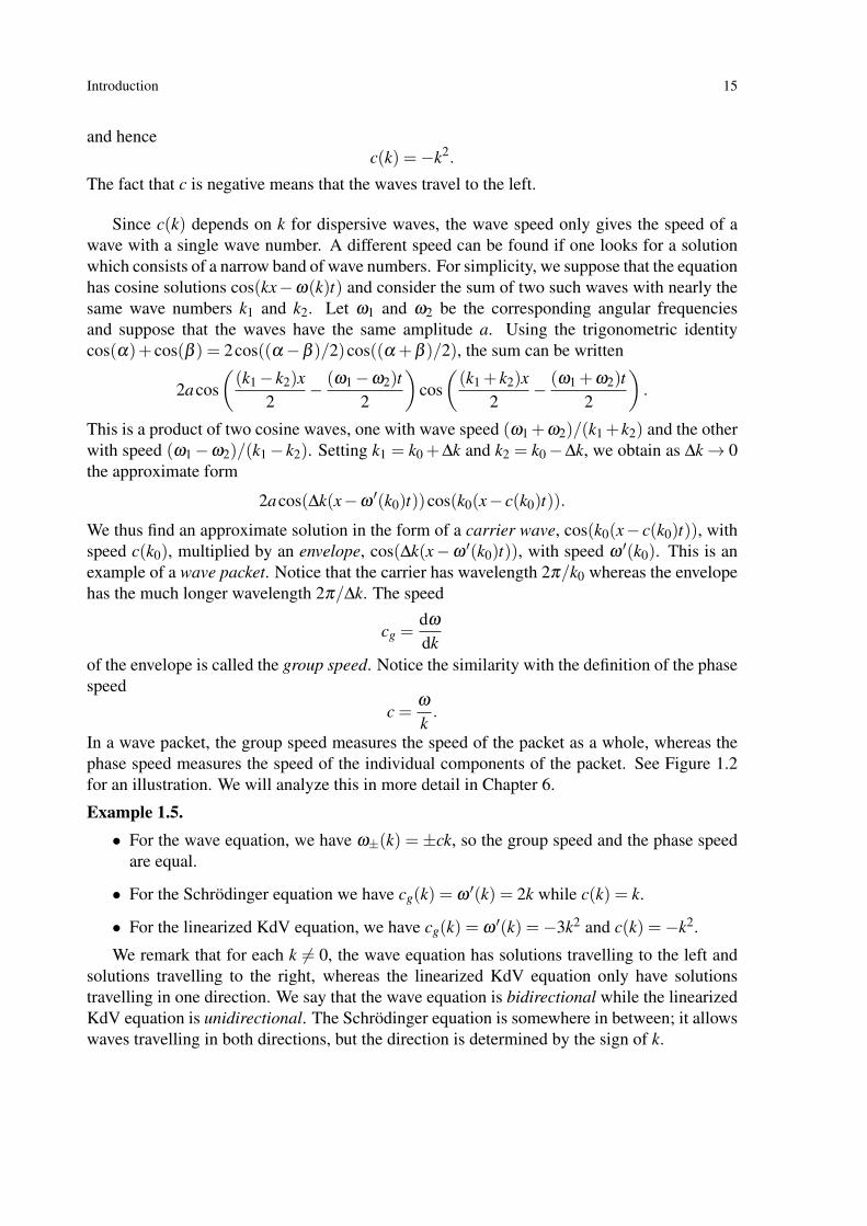
We thus find an approximate solution in the form of a carrier wave, cos(k0(x− c(k0)t)), withspeed c(k0), multiplied by an envelope, cos(∆k(x−ω ′(k0)t)), with speed ω ′(k0). This is anexample of a wave packet. Notice that the carrier has wavelength 2π/k0 whereas the envelopehas the much longer wavelength 2π/∆k. The speed
cg =dω
dkof the envelope is called the group speed. Notice the similarity with the definition of the phasespeed
c =ω
k.
In a wave packet, the group speed measures the speed of the packet as a whole, whereas thephase speed measures the speed of the individual components of the packet. See Figure 1.2for an illustration. We will analyze this in more detail in Chapter 6.
Example 1.5.• For the wave equation, we have ω±(k) = ±ck, so the group speed and the phase speed
are equal.
• For the Schrödinger equation we have cg(k) = ω ′(k) = 2k while c(k) = k.
• For the linearized KdV equation, we have cg(k) = ω ′(k) =−3k2 and c(k) =−k2.
We remark that for each k 6= 0, the wave equation has solutions travelling to the left andsolutions travelling to the right, whereas the linearized KdV equation only have solutionstravelling in one direction. We say that the wave equation is bidirectional while the linearizedKdV equation is unidirectional. The Schrödinger equation is somewhere in between; it allowswaves travelling in both directions, but the direction is determined by the sign of k.

16 Introduction
cg
c
Figure 1.2: A wave packet. The groups speed, cg, is the speed of the packet as a whole, whilethe phase speed c is the speed of the individual crests and troughs.
1.2 Nonlinear wavesThe (inviscid) Burgers equation
ut +uux = 0 (1.3)
is a simplified model for fluid flow. It is named after the Dutch physicist Jan Burgers whostudied the viscous version
ut +uux = εuxx, ε > 0,
(viscosity is the internal friction of a fluid) as a model for turbulent flow. Recalling our discus-sion of the wave equation above, we can think of the Burgers equation as
ut + c(u)ux = 0,
with ‘speed’ c(u) = u. Again, the left hand side can be thought of as a directional derivative inthe direction (u,1), which now depends on u. When studying the equation ut + cux = 0 withconstant c, we found that the solution was constant on straight lines in the direction (c,1).This suggests that the solution of Burgers’ equation should be constant on curves with tangent(u(x, t),1). Such curves are given by (x(t), t), where x(t) is a solution of the differentialequation
x(t) = u(x(t), t).
This doesn’t seem to help much since we don’t know u. However, since u is constant on thecurve, the equation actually simplifies to
x(t) = u0(x0),
where x0 = x(0) and u0(x) = u(x,0). This means that the curves (x(t), t) actually are straightlines,
(x(t), t) = (x0 +u0(x0)t, t),
and that we haveu(x0 +u0(x0)t, t) = u0(x0). (1.4)

Introduction 17
Figure 1.3: The evolution of a positive solution of the Burgers equation. ‘Particles’ locatedhigher up have greater speed. The solution steepens and eventually becomes multivalued. Ofcourse, it is then no longer a function and doesn’t satisfy equation (1.3).
This determines, at least formally, the solution in an implicit way. Note that this gives credenceto our interpretation of u as a speed: considering a ‘particle’ situated originally on the graph ofu at (x0,u0(x0)), this particle will travel parallel to the x-axis with constant speed u0(x0) (theparticle will travel backwards if u0(x0)< 0). This suggests that (1.4) actually does define thesolution implicitly for some time. However, suppose that the function u0 has negative slopesomewhere, so that there exist points x1 < x2 with u0(x1)> u0(x2). We suppose for simplicitythat these values are positive. The point originally located at (x1,u0(x1)) will then have greaterspeed than the point located at (x2,u0(x2)) so that at some point T the solution will develop avertical tangent. Continuing the ‘Lagrangian’1 solution beyond this point in time, the functionu will become multivalued (see Figure 1.3). Clearly, u then ceases to be a solution of theoriginal equation (1.3). In Chapter 4 we will study a different way of continuing the solutionpast the time T , namely as a shock wave. The solution then continues to be the graph of afunction, but now has a jump discontinuity. Clearly, this solution can’t satisfy (1.3) either, andso we have to develop a different way of interpreting solutions.
The above example shows that nonlinear waves may develop singularities. It turns out thatdispersion can sometimes help, however. If we add to the Burgers equation the dispersionterm uxxx, we obtain the famous Korteweg-de Vries (KdV) equation
ut +6uux +uxxx = 0 (1.5)
(the coefficient 6 is inessential). This equation is named after the Dutch mathematicianDiederik Korteweg and his student Gustav de Vries, who derived it as an equation for longwater waves in 1895. The equation had in fact been derived previously by Joseph Boussinesq[3]. As we will show in Chapter 6, the solutions of the KdV equation remain smooth for alltimes. Naively one can think of the nonlinear terms as trying to focus and steepen the wave.The dispersive term on the other hand tends to spread the wave apart and therefore might beable to counteract the nonlinearity.
1In the Lagrangian approach to fluid mechanics, the coordinates follow the fluid particles. In the Eulerianapproach the coordinates are fixed while the fluid moves.

18 Introduction
1.3 SolitonsThe KdV equation was derived in attempt to explain a phenomenon observed earlier by theScottish naval engineer John Scott Russell. In 1834, on the Union canal between Edinburghand Glasgow, Scott Russell made a remarkable discovery. This is his own account of the event[22].
I was observing the motion of a boat which was rapidly drawn along a narrowchannel by a pair of horses, when the boat suddenly stopped—not so the massof water in the channel which it had put in motion; it accumulated round theprow of the vessel in a state of violent agitation; then suddenly leaving it behind,rolled forward with great velocity, assuming the form of a large solitary elevation,a rounded, smooth and well defined heap of water, which continued its coursealong the channel apparently without change of form or diminution of speed. Ifollowed it on horseback, and overtook it still rolling on at a rate of some eightor nine miles an hour, preserving its original figure some thirty feet long and afoot to foot and half in height. Its height gradually diminished, and after a chaseof one or two miles I lost it in the windings of the channel. Such, in the monthof August, 1834, was my first chance interview with that singular and beautifulphenomenon which I have called the Wave of Translation.
As far as we know this is the first reported observation of a solitary water wave. Scott Rus-sell was to spend a great deal of time reproducing the phenomenon in laboratory experiments.He built a small water channel in the end of which he dropped weights, producing solitarybump-like waves of the sort he had earlier observed. Figure 1.4 shows Scott Russell’s ownillustrations of his experiments.
At that time the predominant mathematical theory for water waves was linear. In particular,the esteemed mathematicians and fluid dynamicists Sir George Gabriel Stokes and Sir GeorgeBiddell Airy–both with chairs at University of Cambridge—did not accept Russell’s theories,because they believed that it contradicted the mathematical/physical laws of fluid motion. Infact, if one considers only linear dispersive equations one finds that solitary travelling waves onthe whole line are impossible. For the linearized KdV equation, any wave is the superpositionof periodic travelling waves of different wave numbers which disperse with time.
To explain Scott Russell’s observations, we look for a travelling wave solution of the KdVequation which decays to 0 at infinity. Such a solution is called a solitary wave.2 We thusmake the Ansatz u(x, t) =U(x− ct). This yields the ODE
−cU ′(X)+6U(X)U ′(X)+U ′′′(X) = 0, (1.6)
where X = x− ct. Since we are looking for a solitary wave we also require that
limX→±∞
U(X) = 0. (1.7)
2A solitary wave could also converge to a non-zero constant at infinity.

Introduction 19
Figure 1.4: John Scott Russell’s illustrations of his experiments from [22].

20 Introduction
U
V
Figure 1.5: The phase portrait of (1.9) with c > 0. The thick curve represents the homoclinicorbit corresponding to the solitary wave. The filled circles represent the equilibria (0,0) and(0,c/3).
We may integrate equation (1.6) to
U ′′ = cU−3U2 +C1, C1 ∈ R.
In view of (1.7), we set C1 = 0. Otherwise U ′′ would converge to a non-zero number, yieldinga contradiction. We thus arrive at the second order ODE
U ′′ = cU−3U2. (1.8)
This can be written as the first-order systemU ′ =VV ′ = cU−3U2 (1.9)
and we find that the function
H(U,V ) =V 2− cU2−2U3
is constant on the orbits. We can thus find the phase portrait by drawing the level curves ofH. Moreover, the orbit corresponding to a solitary wave must lie in the level set H−1(0). Thisreveals that we must take c> 0 in order to find a solitary wave. The phase portrait in this case isshown in Figure 1.5. We find that there is a homoclinic orbit connecting the origin with itself.Since the ODE is autonomous, this orbit corresponds to a family of solutions X 7→U(X−X0),X0 ∈ R, of (1.6)–(1.7). We also note from Figure 1.5 that U(X)> 0 for all X .
We can in fact find an explicit formula for U(X). To make U unique, we assume (withoutloss of generality) that U(0) = c/2 and hence U ′(0) =V (0) = 0 (from the equation H(U,V ) =0). Note that
X 7→ (U(−X),−V (−X))

Introduction 21
also is a solution of (1.9) with the same initial data, so that by the Picard-Lindelöf theorem,U(X) =U(−X) (U is even). It therefore suffices to find the solution for X > 0. Also, note thatU(X) ∈ (0,c/2] for all X . The equation H(U,U ′) = 0 can be written
(U ′)2 = cU2−2U3,
which yieldsU ′ =−U
√c−2U ,
for X ≥ 0. This is a separable ODE. For X > 0 we know that U(X)< c/2 and hence
−∫ U(X)
U(X0)
dUU√
c−2U= X−X0, X0 > 0, X > 0,
By continuity this also holds in the limit X0→ 0, so that
−∫ U(X)
c/2
dUU√
c−2U= X , X > 0.
To calculate this integral, we introduce the new variable θ defined by
U =c
2cosh2(θ),
∂U∂θ
=−csinh(θ)cosh3(θ)
, θ > 0.
Note that θ = 0 corresponds to U = c/2 and θ = ∞ to U = 0. The identity cosh2(θ)−sinh2(θ) = 1 implies that
√c−2U =
√c(
1− 1cosh2(θ)
)=
√c(
cosh2(θ)−1cosh2(θ)
)=√
csinh(θ)cosh(θ)
,
and1U
1√c−2U
∂U∂θ
=−2cosh2(θ)
ccosh(θ)√c sinh(θ)
c sinh(θ)cosh3(θ)
=− 2√c.
We therefore obtain that2√c
θ(X) =∫
θ(X)
0
2√c
dθ
=−∫ U(X)
c/2
dUU√
c−2U= X ,
whereU(X) =
c2cosh2(θ(X))
.
It follows that
U(X) =c
2cosh2(√
c2 X) =
c2
sech2(√
c2
X), X ≥ 0, (1.10)
where sech = 1/cosh is the hyperbolic secant. Since U and sech are even, the formula alsoholds for X < 0. Going back to the original variables, we have proved the following result.

22 Introduction
Figure 1.6: The great wave of translation. Three solitary-wave solutions of the KdV equationof the form (1.10). Notice that fast waves are tall and narrow.
Theorem 1.6. For each c > 0 there is a family of solitary-wave solutions
u(x, t) =c2
sech2(√
c2(x− ct− x0)
), x0 ∈ R, (1.11)
of the KdV equation (1.5). For c < 0 there are no solitary wave solutions.
Note that the amplitude is proportional to the wave speed c, so that higher waves travelfaster. The width of the wave3, on the other hand, is inversely proportional to
√c. In other
words, the waves become narrower the taller they are (see Figure 1.6). Another interestingaspect is that the solitary waves move in the opposite direction of the travelling waves of thelinearized KdV equation (cf. Example 1.4). In fact, if one perturbs a solitary wave, one willgenerally see a small ‘dispersive tail’ travelling in the opposite direction.
The KdV equation was largely forgotten about by the mathematical community until the1960’s. In a numerical study of the initial-value problem
ut +uux +δ2uxxx = 0, u(x,0) = cos(πx), (1.12)
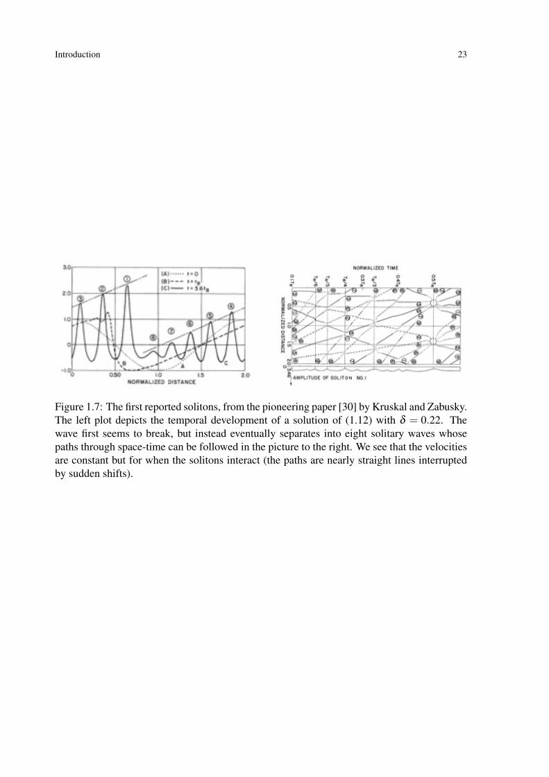
with periodic boundary conditions and δ 6= 0 but small, Martin Kruskal and Norman Zabuskydiscovered that the solution splits up into finitely many distinct waves resembling the sech2-wave, which interacted with each other almost as the equation was linear. They called thewaves solitons. We will investigate this in much more detail in Chapter 7. Figure 1.7 showssome pictures from Kruskal and Zabusky’s original paper.
3The width can e.g. be defined as the distance between to points where the elevation is half of the amplitude,u = c/4.
Introduction 23
!"#$%&'()*+,-./0123456789:;<=>?@ABCDEFGHIJKLMNOPQRSTUVWXYZ[\]_abcdefghijklmnopqrstuvwxyz|~!"#$%&'()*+,-./0123456789:;<=>?@ABCDEFGHIJKLMNOPQRSTUVWXYZ[\]_abcdefghijklmnopqrstuvwxyz|~
Figure 1.7: The first reported solitons, from the pioneering paper [30] by Kruskal and Zabusky.The left plot depicts the temporal development of a solution of (1.12) with δ = 0.22. Thewave first seems to break, but instead eventually separates into eight solitary waves whosepaths through space-time can be followed in the picture to the right. We see that the velocitiesare constant but for when the solitons interact (the paths are nearly straight lines interruptedby sudden shifts).

24 Introduction

Chapter 2
The Fourier transform
2.1 The Schwartz spaceWe begin by studying the Fourier transform on a class of very nice functions. This meansthat we don’t have to worry much about technical details. In order to define this class it ispractical to use the ‘multi-index’ notation due to Laurent Schwartz. Let N = 0,1,2, . . .. Ifα = (α1, . . . ,αd) ∈ Nd , we define
∂αx = ∂
α1x1
∂α2x2· · ·∂ αd
xd.
One can think of ∂x as the d-tuple (∂x1, . . . ,∂xd). We similarly define xα = xα11 · · ·x
αdd for x∈Rd
(or even Cd). The number |α| = α1 + · · ·+αn is called the order of the multi-index and wealso write α! = α1! · · ·αd!. All functions in this chapter are allowed to be complex-valued.
Definition 2.1 (Schwartz space). The Schwartz space S (Rd) is the vector space of rapidlydecreasing smooth functions,
S (Rd) :=
f ∈C∞(Rd) : sup
x∈Rd|xα
∂βx f (x)|< ∞ for all α,β ∈ Nd
.
S (Rd) contains the class of C∞ functions with compact support, C∞0 (Rd). See Lemma
B.24 for a non-trivial example of functions belonging to this class. The main reason forusing S instead of C∞
0 is that, as we will see, the former class is invariant under the Fouriertransform. This is not the case for C∞
0 .
The topology on S (Rd) is defined by the family of semi-norms (see Section A.1),
‖ f‖α,β := supx∈Rd|xα
∂βx f (x)|, α,β ∈ Nd.
In other words, we say thatϕn→ ϕ
in S (Rd) iflimn→∞‖ϕn−ϕ‖α,β = 0
25

26 The Fourier transform
for all α,β ∈ Nd . One can in fact show that
ρ( f ,g) := ∑α,β
12|α|+|β |
‖ f −g‖α,β
1+‖ f −g‖α,β,
defines a metric on S (Rd). The topology defined by this metric is the same as the one definedby the semi-norms and the metric space (S (Rd),ρ) is complete. S (Rd) is an example ofa generalization of Banach spaces called Frechét spaces, but we will not use that in any sub-stantial way. Notice, though, that the Schwartz space is not a Banach space, i.e. it cannot beequipped with a norm making it complete (in particular, f 7→ ρ( f ,0) does not define a norm).
Proposition 2.2.
(1) For all N ≥ 0 and α ∈Nd there exists a C > 0 such that |∂ αx f (x)| ≤C(1+ |x|)−N , x∈Rd .
(2) S (Rd) is closed under multiplication by polynomials.
(3) S (Rd) is closed under differentiation.
(4) S (Rd) is an algebra: f g ∈S (Rd) if f ,g ∈S (Rd).
(5) C∞0 (Rd) is a dense subspace of S (Rd).
(6) S (Rd) is a dense subspace of Lp(Rd) for 1≤ p < ∞.
Proof. The first property is basically a restatement of the definition of S (Rd). Properties (2)and (3) follow from the definition of the Schwartz space. Property (4) is a consequence ofLeibniz’ formula for derivatives of products.
It is clear that C∞0 (Rd) ⊂ S (Rd). To show that it is dense, let f ∈ S (Rd) and define
fn(x) = ϕ(x/n) f (x), where ϕ ∈C∞0 (Rd) with ϕ(x) = 1 for |x| ≤ 1 (see Lemma B.24). Then
fn− f = (ϕ(x/n)−1) f (x)
with support in Rd \Bn(0). From property (1) it follows that | f (x)| ≤CN(1+ |x|)−N for anyN ≥ 0. Therefore
‖ fn− f‖L∞(Rd) ≤CN(1+‖ϕ‖L∞(Rd))(1+n)−N → 0
as n→ ∞. Since N is arbitrary, the same is true if we multiply fn− f by a polynomial. Sincethe partial derivatives of ϕ(x/n)−1 all have support in Rd \Bn(0) and are bounded uniformlyin n, the convergence remains true after differentiation. This proves (5).
By estimating| f (x)| ≤C(1+ |x|)−d−1
and using the fact that∫Rd(1+ |x|)−p(d+1) dx =C
∫∞
0
rd−1
1+ rp(d+1)dr < ∞,

The Fourier transform 27
it follows that f ∈ Lp(Rd) for 1 ≤ p < ∞, if f ∈S (Rd). Since C∞0 (Rd) is dense in Lp(Rd)
(cf. Corollary B.26), property (6) now follows from property (5) (we only use the part thatC∞
0 (Rd)⊂S (Rd)).
Example 2.3. The Gaussian function e−|x|2
is an example of a function in S (Rd) which isnot in C∞
0 (Rd).
2.2 The Fourier transform on S
Definition 2.4 (Fourier transform). The Fourier transform, F ( f ), of a function f ∈S (Rd)is defined by
F ( f )(ξ ) =1
(2π)d/2
∫Rd
f (x)e−ix·ξ dx. (2.1)
We also use the notation f = F ( f ).
It is clear from the inequality∣∣∣∣∫Rdf (x)e−ix·ξ dx
∣∣∣∣≤ ∫Rd| f (x)|dx (2.2)
and Proposition 2.2 (6) that f (ξ ) is defined for each ξ ∈ Rd .
Lemma 2.5. Let f ∈S (Rd). Then f is a bounded continuous function with
‖ f‖L∞(Rd) ≤ (2π)−d/2‖ f‖L1(Rd)
Proof. The boundedness follows directly from the inequality (2.2). The continuity is a conse-quence of the dominated convergence theorem (see Theorem B.15).
Proposition 2.6. For f ∈S (Rd), we have that f ∈C∞(Rd) and
f (x+ y) F7→ eiy·ξ f (ξ ),
eiy·x f (x) F7→ f (ξ − y),
f (Ax) F7→ |detA|−1 f (A−Tξ )
f (λx) F7→ |λ |−d f (λ−1ξ ),
∂αx f (x) F7→ (iξ )α f (ξ ),
xα f (x) F7→ (i∂ξ )α f (ξ ),
where y ∈ Rd , λ ∈ R\0 and A is an invertible real d×d matrix.

28 The Fourier transform
Proof. The first four properties follow by changing variables in the integral in (2.1). The fifthproperty follows by partial integration and the sixth by differentiation under the integral sign.This also proves that f ∈C∞(Rd).
Example 2.7. Let us compute the Fourier transform of the Gaussian function e−|x|2/2, x ∈Rd .
We begin by considering the case d = 1. The function u(x) = e−x2/2 satisfies the differentialequation u′(x) =−xu(x). Taking Fourier transforms we therefore find that iξ u(ξ ) =−iu′(ξ ),or equivalently u′(ξ ) =−ξ u(ξ ). But this means that
u(ξ ) =Ce−ξ 22 ,
where
C = u(0) =1√2π
∫R
e−x22 dx.
This integral can be computed using the standard trick
C2 =1
2π
∫∫R2
e−(x2+y2)
2 dxdy
=∫
∞
0e−
r22 r dr
= 1.
Since C > 0 it follows that C = 1. Hence,
F (e−x22 )(ξ ) = e−
ξ 22 ,
that is, u is invariant under the Fourier transform!This can be generalized to Rd , since
e−|x|2/2 =
d
∏j=1
e−x2j/2, x = (x1, . . . ,xd) ∈ Rd.
From this it follows that
F (e−|x|2/2)(ξ ) =
d
∏j=1
F (e−x2j/2)(ξ j) =
d
∏j=1
e−ξ 2j /2 = e−|ξ |
2/2.
Note in particular that the Fourier transform of a Gaussian function is in S (Rd). This isno coincidence.
Theorem 2.8. For any f ∈S (Rd), F ( f ) ∈S (Rd), and F is a continuous transformationof S (Rd) to itself.

The Fourier transform 29
Proof. We estimate the S (Rd) semi-norms of f as follows:
‖ f‖α,β = ‖ξ α∂
β
ξf‖L∞(Rd)
= ‖F (∂ αx (xβ f ))‖L∞(Rd)
≤ (2π)−d/2‖∂ αx (xβ f )‖L1(Rd)
= (2π)−d/2‖(1+ |x|)−(d+1)(1+ |x|)d+1∂
αx (xβ f )‖L1(Rd)
≤C‖(1+ |x|)d+1∂
αx (xβ f )‖L∞(Rd).
The last line can be estimated by a finite number of semi-norms of f using Leibniz’ formula.It follows that F maps S (Rd) to itself continuously.
Recall that the convolution of two functions f and g is defined by
( f ∗g)(x) :=∫Rd
f (x− y)g(y)dy, (2.3)
whenever this makes sense (see Section B.5).
Theorem 2.9 (Convolution theorem). Let f ,g ∈S (Rd). Then f ∗g = (2π)d/2 f g.
Proof. Using Fubini’s theorem, we have that
(2π)d/2F ( f ∗g)(ξ ) =∫Rd
(∫Rd
f (x− y)g(y)dy)
e−ix·ξ dx
=∫Rd
(∫Rd
f (x− y)e−ix·ξ dx)
g(y)dy
=∫Rd
(∫Rd
f (z)e−i(z+y)·ξ dz)
g(y)dy
=
(∫Rd
f (z)e−iz·ξ dz)(∫
Rdg(y)e−iy·ξ dy
)= (2π)d f (ξ ) g(ξ ).
The inverse Fourier transform is defined by
F−1( f )(x) = F ( f )(−x) =1
(2π)d/2
∫Rd
f (x)eix·ξ dx. (2.4)
It is clearly also continuous on S (Rd). The name is explained by the following theorem.
Theorem 2.10 (Fourier’s inversion formula). Let f ∈S (Rd). Then f (x) = F−1( f )(x).
Proof. Let K(x) = (2π)−d/2e−|x|2/2 and recall from Example 2.7 that K = K. In particular,
this implies that∫Rd K(x)dx = (2π)d/2K(0) = 1. By assumption, the iterated integral
1(2π)d/2
∫Rd
(∫Rd
f (y)e−iy·ξ dy)
eix·ξ dξ

30 The Fourier transform
exists for all x ∈ Rd . Squeezing a Gaussian in makes it absolutely convergent, and
fε(x) :=∫Rd
f (ξ )eix·ξ K(εξ )dξ
→ 1(2π)d/2
∫Rd
f (ξ )eix·ξ dξ as ε → 0, (2.5)
by the dominated convergence theorem. Changing order of integration, we also see that
fε(x) =1
(2π)d/2
∫∫Rd×Rd
f (y)ei(x−y)·ξ K(εξ )dydξ
=1
(2π)d/2
∫Rd
f (y)(∫
Rde−i(y−x)·ξ K(εξ )dξ
)dy
=∫Rd
f (y)F (K(εξ ))(y− x)dy
= ε−d∫R
f (y)K(ε−1(y− x))dy
= (Kε ∗ f )(x),
where Kε(x) = ε−dK(ε−1x). Theorem B.27 implies that
limε→0
fε(x) = f (x). (2.6)
The result follows by combining (2.5) and (2.6).
Corollary 2.11. The Fourier transform is a linear bijection of S (Rd) to itself with inverseequal to F−1. That is,
F−1F = FF−1 = Id on S (Rd).
Proof. The above results implies that F−1F = Id on S (Rd). To prove the corollary, wemust also show that FF−1 = Id. Define the reflection operator R : S (Rd)→ S (Rd) byR( f )(x) = f (−x). R commutes with F and F−1 (Proposition 2.6), is its own inverse andsatisfies F−1 = RF . It follows that
FF−1 = FRF = F−1F = Id .
Corollary 2.12. Let f ,g ∈S (Rd). Then f ∗g ∈S (Rd).
Proof. This follows from the convolution theorem, Fourier’s inversion formula and the factthat S (Rd) is an algebra, since f ∗g = (2π)d/2F−1( f g).

The Fourier transform 31
2.3 Extension of the Fourier transform to Lp
Since S (Rd) is dense in Lp(Rd) for 1≤ p < ∞ (Proposition 2.2), it is natural to try to extendthe Fourier transform to Lp by continuity. We have the following abstract result.
Proposition 2.13. Suppose that X is a normed vector space, E ⊂ X is a dense linear subspace,and Y is a Banach space. If T : E → Y is a bounded linear operator in the sense that thereexists C > 0 such that
‖T x‖Y ≤C‖x‖X
for each x ∈ E, then there is a unique bounded extension T : X → Y of T .
Proof. Let S be another bounded extension. If x ∈ X and xn is a sequence in E whichconverges to X , we find that
limn→∞
(T −S)xn = (T −S)x,
while at the same time(T −S)xn = (T −T )xn = 0.
It follows that T x = Sx.To prove the existence of T , let x and xn be as above. Then xn is a Cauchy sequence in
X . Since T is bounded it follows that T xn is a Cauchy sequence in Y . By completeness of Ythere exists a limit, which we define to be T x. The limit is clearly independent of the sequencexn since T applied to the difference of two such sequence will converge to 0. Linearity andboundedness follow by a limiting procedure.
We begin by extending the Fourier transform to L1. This extension can in fact be definedwithout using the above proposition. In order to simplify the notation, we also write f =F ( f )for the extension. Let Cb(Rd) be the space of bounded continuous functions on Rd , equippedwith the supremum norm.
Theorem 2.14 (Riemann-Lebesgue lemma). F : S (Rd)→ S (Rd) extends uniquely to abounded linear operator L1(Rd) → Cb(Rd), defined as the absolutely convergent integral(2.1). Moreover,
‖ f‖L∞(Rd) ≤ (2π)−d/2‖ f‖L1(Rd) (2.7)
and limx→∞ f (x) = 0.
Proof. Repeating the proof of Lemma 2.5, we find that the extension exists and defines abounded operator satisfying the estimate (2.7). Proposition 2.13 shows that it is unique.To prove that f (x) → 0 as x → ∞, we take ε > 0 and g ∈ S (Rd) with ‖ f − g‖L∞(Rd) ≤(2π)−d/2‖ f −g‖L1(Rd) < ε/2. Choosing R large enough, we find that |g(x)|< ε/2 for |x| ≥ R.Hence,
| f (x)| ≤ ‖ f − g‖L∞(Rd)+ |g(x)|< ε
for |x| ≥ R.
In order to extend the Fourier transform to L2(Rd), we need an estimate similar to (2.7).In fact, we can do even better.

32 The Fourier transform
Lemma 2.15. For f ,g ∈S (Rd), we have that
(F ( f ),g)L2(Rd) = ( f ,F−1(g))L2(Rd),
where( f ,g)L2(Rd) =
∫Rd
f (x)g(x)dx
is the inner product on L2(Rd).
Proof. Just as in the proof of Theorem 2.9, we use Fubini’s theorem to change the order ofintegration: ∫
RdF ( f )(x)g(x)dx =
∫Rd
(∫Rd
f (y)e−ix·y dy)
g(x)dx
=∫Rd
(∫Rd
g(x)eix·y dx)
f (y)dy
=∫Rd
f (y)F−1(g)(y)dy.
In particular, if f ,g ∈S (Rd), one finds that
(F ( f ),F (g))L2(Rd) = ( f ,F−1F (g))L2(Rd) = ( f ,g)L2(Rd) (2.8)
by Fourier’s inversion theorem. Taking g = f , we find that
‖F ( f )‖2L2(Rd) = ‖ f‖2
L2(Rd) = ‖F−1( f )‖2
L2(Rd), (2.9)
where the last equality follows from the first by replacing f with F−1( f ). This is sometimescalled Parseval’s formula. A bijective linear operator which preserves the inner product iscalled a unitary operator. Note that a unitary operator automatically is bounded.
Theorem 2.16 (Plancherel’s theorem). The Fourier transform F and the inverse Fouriertransform F−1 on S (Rd) extend uniquely to unitary operators on L2(Rd) satisfying F−1F =FF−1 = Id.
Proof. The existence and uniqueness of the extensions follow from Proposition 2.13 and (2.9).Since FF−1 = F−1F = Id on a dense subspace, it follows that the same is true on L2(Rd).By continuity, we have that (F ( f ),g)L2(Rd) = ( f ,F−1(g))L2(Rd) for f ,g ∈ L2(Rd), so F andF−1 are unitary.
Since the Fourier transform is defined for L1(Rd) and L2(Rd), one can in fact extend it toLp(Rd), 1≤ p≤ 2, by interpolation. The following result is a direct consequence of Theorems2.14, 2.16 and B.28.
Theorem 2.17 (Hausdorff-Young inequality). Let p∈ [1,2] and q∈ [2,∞] with 1p +
1q = 1. The
Fourier transform extends uniquely to a bounded linear operator F : Lp(Rd)→ Lq(Rd), with
‖F ( f )‖Lq(Rd) ≤ (2π)d2
(1− 2
p
)‖ f‖Lp(Rd), f ∈ Lp(Rd).

The Fourier transform 33
The extension to Lp(Rd) for p > 2 is a completely different matter. We will return to thisin Chapter 5.
Note that many of the properties of the Fourier transform on S (Rd) automatically hold onLp(Rd), 1 ≤ p ≤ 2, by continuity. This is e.g. true for the four first properties in Proposition2.6. One also obtains the following extension of Fourier’s inversion formula.
Proposition 2.18. Let f ∈ Lp(Rd) for some p ∈ [1,2] and f ∈ L1(Rd). Then f is continuous1
and f (x) = F−1( f )(x) for all x ∈ Rd .
Note that we have defined the extension in two different ways if e.g. f ∈ L1(Rd)∩L2(Rd).However, approximating f by a sequence in fn in C∞
0 (Rd) with fn→ f in L1 and L2, we findthat fn→FL1( f ) in Cb and fn→FL2( f ) in L2, where the subscripts on the Fourier transformsare used to differentiate the two extensions. But this implies that FL2( f ) = FL1( f ) a.e.
Example 2.19. Let
f (x) =
1, x ∈ [−1,1],0, x 6∈ [−1,1]
be the characteristic function of the interval [−1,1]. f ∈ L1(R), so
f (ξ ) =1√2π
∫R
f (x)e−ixξ dx
=1√2π
∫ 1
−1e−ixξ dx
=1√2π
[e−ixξ
−iξ
]1
x=−1
=1√2π
eiξ − e−iξ
iξ
=
√2π
sin(ξ )ξ
.
f is not in L1(R), so we can’t use the pointwise inversion formula in Proposition 2.18. We dohowever have f =F−1( f ) in the sense of Theorem 2.16 since f ∈ L2(R). Moreover, we have
‖ f‖2L2(Rd) = ‖ f‖2
L2(Rd),
by Parseval’s formula. When written out, this means that∫R
sin2ξ
ξ 2 dξ = π.
1Meaning that there is an element of the equivalence class which is continuous.

34 The Fourier transform

Chapter 3
Linear PDE with constant coefficients
In this chapter we will study the simplest kind of PDE, namely linear PDE with constant coef-ficients. This means in particular that the superposition principle holds, so that new solutionscan be constructed by forming linear combinations of known solutions. There are two mainreasons for why this chapter is included in the lecture notes. The first reason is that someimportant equations describing waves are linear. The second is that many nonlinear waveequations can be treated as perturbations of linear ones. A knowledge of linear equations istherefore essential for understanding nonlinear problems.
We will concentrate on the Cauchy problem (the initial-value problem), in which, in ad-dition to the PDE, the values of the unknown function and sufficiently many time derivativesare prescribed at t = 0. This presupposes that there is some distinguished variable t which canbe interpreted as time. Usually this is clear from the physical background of the equation inquestion. If you are familiar with the Cauchy problem for ordinary differential equations youknow that there always exists a unique solution under sufficient regularity hypotheses. Wewill look for conditions under which the same property is true for PDE. Our goal is in fact toconvert the PDE to ODE by using the Fourier transform with respect to the spatial variablesx. From now on, Fourier transforms will only be applied with respect to the spatial variables.We will consider functions u(x, t) defined for all x ∈ Rd . This is of course a simplification;in the ‘physical world’, u(x, t) will only be defined for x in some bounded domain and therewill be additional boundary conditions imposed on the boundary of this domain. Our studywill not be completely restricted to equations describing waves, but in the end we will arriveat a condition which guarantees that the solutions behave like waves in the sense that thereis a well-defined speed of propagation. Equations having this property are called hyperbolic.Not all equations which describe waves are hyperbolic. In particular, dispersive equationssuch as the Schrödinger equation and the linearized KdV equation are not. Nevertheless, wewill prove that the Cauchy problem is uniquely solvable for these equations as well. Furtherproperties of dispersive equations will be studied in Chapter 6.
We begin by considering three classical second order equations, namely the heat equation,the wave equation and the Laplace equation. These examples are instructive in that they illus-trate that the properties of the solutions of PDE depend heavily on the form of the equation.They also give us some intuition of what to expect in general.
35

36 Linear PDE with constant coefficients
The presentation of the material in this chapter is close that in Rauch [20]. The treatmentof Kirchhoff’s solution formula for the wave equation in R3 follows Stein and Shakarchi [24].A more detailed account of the theory of linear PDE with constant coefficients can be foundin Hörmander [13].
3.1 The heat equation
3.1.1 Derivation
The heat equation in R3 is the equation
ut = k∆u, (3.1)
where ∆u = ∂ 2x1
u+ ∂ 2x2
u+ ∂ 2x3
u and k > 0 is a constant. As the name suggest, the equationdescribes the flow of heat. Recall that heat is a form of energy transferred between two bodies,or regions of space, at different temperatures. Heat transfer to a region increases or decreasesthe internal energy in that region. The internal energy of a system consists of all the differentforms of energy of the molecules in the system, but excludes the energy associated with themovement of the system as a whole. We look at this from a macroscopic perspective andsuppose that the internal energy can be described by a density e(x, t). If E(t) is the totalinternal energy in the domain Ω⊂ R3 we therefore have that
E(t) =∫
Ω
e(x, t)dx,
and the rate of change is
E ′(t) =∫
Ω
et(x, t)dx.
The heat flux J is a vector-valued function which describes the flow of heat. The total transferof heat across an oriented surface Σ is given by∫
Σ
J(x, t) ·n(x)dS(x),
where n denotes the unit normal and dS the element of surface area on Σ. The rate at whichheat leaves Ω is therefore
∫∂Ω
J ·ndS, where n is the outer unit normal. Using the divergencetheorem, this can be rewritten as
∫Ω
∇ ·J dx. Assuming that the only change in internal energyis due to conduction of heat across the boundary, we find that∫
Ω
(et +∇ · J)dx = 0.
Since this holds for all sufficiently nice domains Ω we obtain the continuity equation
et +∇ · J = 0

Linear PDE with constant coefficients 37
if all the involved functions are continuous. To derive the heat equation we use two constitutivelaws. First of all, we assume that over a sufficiently small range of temperatures, e dependslinearly on the temperature T , that is,
e = e0 +ρc(T −T0),
where ρ is the density, c is the specific heat capacity and T0 a reference temperature. Weassume that ρ and c are independent of T . We can simply think of the temperature as whatwe measure with a thermometer. On a microscopic level, the temperature is a measure ofthe average kinetic energy of the molecules. The above assumption means that an increase ininternal energy results in an increase in temperature. This is not always true, as an increasein internal energy may instead result in an increase in potential energy. This is e.g. whathappens in phase transitions. The second constitutive law is Fourier’s law, which says thatheat flows from hot to cold regions proportionally to the temperature gradient. In other words,J =−κ∇T , where κ is a scalar quantity called the thermal conductivity. Assuming that c andρ are independent of t, we therefore obtain the equation
cρTt = ∇ · (κ∇T ).
If in addition c, ρ and κ are constant, we find that the temperature satisfies the heat equationwith k = κ/(cρ).
The heat equation is sometimes also called the diffusion equation. The physical interpreta-tion is then that u describes the concentration of a substance in some medium (e.g. a chemicalsubstance in some liquid). Diffusion means that the substance tends to move from regionsof higher concentration to regions of lower concentration. The heat equations is obtained byassuming that the rate of motion is proportional to the concentration gradient (Fick’s law ofdiffusion).
3.1.2 Solution by Fourier’s methodThe Cauchy problem for the heat equation in Rd reads
ut(x, t) = ∆u(x, t), t > 0,u(x,0) = u0(x),
(3.2)
where u : Rd × [0,∞)→ C and u0 : Rd → C. Note that one can assume that k = 1 in (3.1)by using the transformation t 7→ kt. It is useful to first consider a solution in the form of anindividual Fourier mode u(t)eiξ ·x. Substituting this in the equation yields
u′(t) =−|ξ |2u(t).
This is an ODE with solution u(t) = e−|ξ |2t u(0). The corresponding solution is therefore
u(x, t) = u(0)e−|ξ |2teix·ξ = u(0)ei(x·ξ+i|ξ |2). (3.3)

38 Linear PDE with constant coefficients
This is written in the form of a complex sinusoidal wave aei(x·ξ−ω(ξ )t) considered in Chapter1, except that the angular frequency ω(ξ ) =−i|ξ |2 now is imaginary. This implies that the ab-solute value of the solution is strictly decreasing in t. Since there are no temporal oscillations,we don’t normally think of the heat equation as an equation describing waves.
Our strategy for solving the Cauchy problem in general is to find a solution which is a‘continuous linear combination’ of solutions of the form (3.3), that is, a Fourier integral inx. We work formally and assume that u and u0 are sufficiently regular, so that their Fouriertransforms are well-defined. We also assume that we can differentiate under the integral sign,so that ∂tF (u) = F (∂tu). We then obtain the transformed problem
ut(ξ , t) =−|ξ |2u(ξ , t), t > 0,u(ξ ,0) = u0(ξ ),
with solution u(ξ , t) = e−t|ξ |2 u0(ξ ). Applying the inverse Fourier transform, we obtain that
u(x, t) =1
(2π)d/2
∫Rd
eix·ξ e−t|ξ |2 u0(ξ )dξ , t ≥ 0. (3.4)
The integral will in general not converge for t < 0 due to the exponentially growing factore−t|ξ |2 . Under the assumption that u0 ∈S (Rd), one can differentiate under the integral sign asmany times as one likes for t > 0 by Theorem B.15. This still is true if we only allow one-sidedtime derivatives at t = 0. It follows that u defined by this formula belongs to C∞(Rd× [0,∞))1.Carrying out the differentiation one also verifies that u satisfies the heat equation and theinitial condition. Since we have derived an explicit formula, it follows that the solution isunique whenever the steps involved in deriving the formula can be justified. This holds e.g.if u(·, t),ut(·, t) ∈ S (Rd) for each t ≥ 0 and u(·, t) and ut(·, t) can be dominated by someL1 functions which are independent of t, so that Theorem B.15 applies. There is however amore natural condition which guarantees that the steps can be justified. The idea is to take theanalogy with ordinary differential equations one step further and think of the solution u as afunction of t with ’values’ in the function space S (Rd).
Definition 3.1. Let I be an open interval in R.
(1) A function u : I→S (Rd) is said to be continuous if ‖u(t +h)−u(t)‖α,β → 0 as h→0 for every semi-norm ‖ · ‖α,β and every t ∈ I. C(I;S (Rd)) is the vector space ofcontinuous functions I→S (Rd).
(2) A function u : I→S (Rd) is said to be differentiable with derivative u′ : I→S (Rd) if
limh→0
∥∥∥∥u(t +h)−u(t)h
−u′(t)∥∥∥∥
α,β
= 0
for all α,β ∈Nd and t ∈ I. The space C1(I;S (Rd)) consists of differentiable functionsu : I→S (Rd) such that u,u′ ∈C(I;S (Rd)).
1Meaning that at t = 0 derivatives with respect to t are only taken from the right.

Linear PDE with constant coefficients 39
(3) The space Ck(I;S (Rd)), k≥ 2, is defined inductively by requiring that u∈C(I;S (Rd))and u′ ∈Ck−1(I;S (Rd)), and C∞(I;S (Rd)) = ∩∞
k=0Ck(I;S (Rd)).
If I is any interval (not necessarily open), we say that u∈Ck(I;S (Rd)) if it is k times continu-ously differentiable from the interior of I to S (Rd) and all the derivatives extend continuouslyin S (Rd) to the endpoints.
A function u ∈C(I;S (Rd)) also defines a function v ∈Rd× I→C, v(x, t) = u(t)(x). Thedefinition implies that v ∈C(Rd× I) and that v(·, t) ∈S (Rd) for each t ∈ I. When there is norisk of confusion we shall write u for v. Also, to clarify the notation, we will write ut or ∂tu foru′. If u∈C1(I;S (Rd)) it follows in particular that t 7→ ∂ α
x u(x, t) is continuously differentiableon I for each α ∈ Nd and each fixed x ∈ Rd .
Lemma 3.2. Assume that u∈Ck(I;S (Rd)). Then u∈Ck(I;S (Rd)) with ∂ kt F (u)=F (∂ k
t u).
Proof. The result follows immediately from Lemma 2.8.
We therefore obtain uniqueness in the class C∞([0,∞);S (Rd)) for instance. The fact thatthe solution u given by (3.4) belongs to this class follows immediately from the fact thatt 7→ u0(ξ )e−t|ξ |2 does so and Lemma 3.2.
There is a final important property to discuss. In real life it is impossible to measure some-thing with infinite accuracy. It is therefore essential that the solution depends continuously onthe data in some sense, so that small measuring errors don’t grow large (at least in finite time).In the case of the heat equation, we e.g. have that the map
S (Rd) 3 u0 7→ u ∈C∞([0,∞);S (Rd))
is continuous if the space C∞([0,∞);S (Rd)) is equipped with the countable family of semi-norms
sup0≤t≤n
‖∂ kt u(·, t)‖α,β , n,k ∈ N,α,β ∈ Nd.
Note that t 7→ ‖∂ kt u(·, t)‖α,β is a continuous function so that the supremum is finite. The
continuity of the map u0 7→ u follows from the formula u(ξ , t) = e−t|ξ |2 u0(ξ ).
In summary, we have proved the following result.
Theorem 3.3. There exists a unique solution u ∈C∞([0,∞);S (Rd)) of the Cauchy problem(3.2). Moreover, the solution map S (Rd) 3 u0 7→ u ∈C∞([0,∞);S (Rd)) is continuous.
A convenient way of describing the solution is by looking at the map S(t) : S (Rd)→S (Rd) from the data u0 to the solution u(·, t) at time t ≥ 0. S is called the propagator forthe heat equation. The continuous dependence of the solution on the initial data means thatS(·) ∈C(S (Rd);C∞([0,∞);S (Rd))). The map S has two important properties. First of all,
S(0) = Id, (3.5)
40 Linear PDE with constant coefficients
where Id is the identity map on S (Rd). Secondly, note that the heat equation is invariant undertranslations in t. This means that the solution with initial data u0 at t = t0 is given by S(t−t0)u0,t ≥ t0. Consider the solution u with initial data u0 at time 0. If s, t ≥ 0 we can express u(·,s+t)in two different ways. We can of course express it as S(s+ t)u0. On the other hand, we cansolve the equation up to time t, which gives us S(t)u0. We can then use this as our new initialdata and solve up to time s+ t. In other words S(s+ t)u0 = S(s+ t− t)S(t)u0 = S(s)S(t)u0. Inother words,
S(s+ t) = S(s)S(t), s, t ≥ 0. (3.6)
Definition 3.4. Let X be a vector space. A family of linear operators S(t)t≥0 on X with theproperties (3.5) and (3.6) is called a semigroup. If the family is defined for all t ∈ R and (3.6)holds for all s, t ∈ R it is called a group.
3.1.3 The heat kernel
Define the heat kernel
Kt(x) :=1
(4πt)d/2 e−|x|24t , t > 0.
Using the convolution theorem and the fact that
F−1(e−t|·|2)(x) =1
(2t)d/2 e−|x|24t = (2π)d/2Kt(x), t > 0
(see Example 2.7), we can express the solution of the heat equation without using the Fouriertransform.
Theorem 3.5. The unique solution of (3.2) with u0 ∈S (Rd) is given by
u(x, t) = (Kt ∗u0)(x), t > 0, (3.7)
where Kt is the heat kernel.
Note that (x, t) 7→Kt(x) is itself a solution of the heat equation in the half space Rd×(0,∞)with (t 7→Kt)∈C∞((0,∞);S (Rd)). Solving the heat equation with initial data Kt we thereforefind that
Ks ∗Kt = Ks+t , s, t > 0.
This is another way of stating the semigroup property of the propagator S(t). We also notethat
‖Kt‖L1(Rd) =∫Rd
Kt(x)dx = (2π)d/2F (Kt)(0) = 1.
Linear PDE with constant coefficients 41
3.1.4 Qualitative propertiesDecay in time
The solutions of the heat equation decay as t → ∞. Physically, this is related to the fact thatheat flows from hot regions to cold regions, so that the temperature evens out. Since we areworking in the whole space Rd and assume that the solutions converge to 0 at spatial infinity,the temperature will converge to 0 everywhere as t→ ∞. The total internal energy is howeverconserved. Mathematically this is reflected in the conservation law∫
Rdu(x, t)dx = (2π)d/2u(0, t) = (2π)d/2u0(0).
The L2 norm decays to zero however.
Proposition 3.6. Assume that u0 ∈S (Rd) and let u be the corresponding solution of (3.2).Then
limt→∞‖u(·, t)‖L2 = 0.
Proof. Using Parseval’s formula it follows that
‖u(·, t)‖2L2 =
∫Rd
e−2t|ξ |2 |u0(ξ )|2 dξ .
Since e−2t|ξ |2 → 0 monotonically as t→ ∞, the proposition follows.
The L2 norm of the solution or its derivative can often be interpeted as some form ofenergy. Due to the above result, one often thinks of the heat equation as a dissipative equation,meaning that energy is lost. This is not true in the physical sense however, since the physicalenergy is given by the conserved quantity
∫Rd u(x, t)dx. From a mathematical point of view,
it is however useful to think of the heat equation as dissipative, in contrast to e.g. the waveequation (see Section 3.2.4).
One can also use the heat kernel to prove the decay of the solution as t → ∞. Using (3.7)and Young’s inequality one can prove a number of estimates.
Proposition 3.7. Assume that u0 ∈S (Rd) and let u be the corresponding solution of (3.2).All the norms ‖u(·, t)‖Lp , p≥ 1, are decreasing functions of t. For p > 1, we have that
limt→∞‖u(·, t)‖Lp = 0.
Proof. Due to the translation invariance in t, it suffices to show that ‖u(·, t)‖Lp ≤ ‖u0‖Lp toprove the monotonicity of the Lp norm. This bound follows from Young’s inequality (TheoremB.29):
‖u(·, t)‖Lp ≤ ‖Kt‖L1‖u0‖Lp = ‖u0‖Lp.
The second part also follows from Young’s inequality:
‖u(·, t)‖Lp ≤ ‖Kt‖Lp‖u0‖L1 =Ct−d2
(1− 1
p
)‖u0‖L1 → 0
if p > 1, for some constant C > 0.

42 Linear PDE with constant coefficients
We mention an alternative way of proving the monotonicity. This is especially useful if onewants to consider the heat equation in a domain other than Rd , where the Fourier transform isnot avaiable. For simplicity we assume that u0 (and hence u) is real-valued. Multiplying theequation ut = ∆u by u and integrating we find that
ddt
(∫Rd
u2 dx)= 2
∫Rd
uut dx = 2∫Rd
u∆udx =−2∫Rd|∇u|2 dx≤ 0
where we used integration by parts in the last step. The monotonicity of the other Lp norms,1 ≤ p < ∞ can be proved in a similar way, although special care has to be taken in the case1 ≤ p < 2 due to regularity problems. The method of multiplying the equation by somequantity and integrating to obtain a bound is called the energy method. One can sometimesguess the form of the integral directly.
Smoothing
The heat equation also has a smoothing property. Again this makes sense physically. Sincethe heat tends to spread out evenly, we expect discontinuities to be ‘evened out’. To formalizethis smoothing property we need to consider non-smooth initial data.
Proposition 3.8. The propagator S(t) : S (Rd)→S (Rd), t ≥ 0, extends uniquely to a con-tinuous map S(t) : Lp(Rd)→ Lp(Rd) for 1≤ p < ∞, given by
S(t)u0 = Kt ∗u0, t > 0
and S(0)u0 = u0.
Proof. It follows from Young’s inequality that Kt ∗ u0 is defined for t > 0 and defines a con-tinuous extension of S(t) : S (Rd)→S (Rd). The uniqueness follows from Propositions 2.13and 3.7.
Proposition 3.9. Let u0 ∈ Lp(Rd), 1 ≤ p < ∞. Then S(·)u0 ∈ C∞(Rd × (0,∞)) and S(t)u0solves the heat equation for t > 0. Moreover, S(t)u0→ u0 in Lp(Rd).
Proof. This follows by using the formula S(t)u0 = Kt ∗ u0. Since Kt(x) is exponentially de-caying in x for t > 0, we can apply Theorem B.15 to differentiate under the integral sign asmany times as we like. It follows that S(t)u0 is smooth in Rd × (0,∞). The convergence ofS(t)u0 = Kt ∗u0 to u0 in Lp is a consequence of Theorem B.27.
Infinite speed of propagation
Suppose that u0 ≥ 0. Formula (3.7) then shows that u(x, t) ≥ 0 for t > 0 and all x ∈ R. Infact it also shows that u(x, t) > 0 unless u0 ≡ 0. This holds even if u0 has compact support.We say that heat equation has infinite speed of propagation. In fact, a much stronger propertyholds. One can show that u is a real analytic function for t > 0, that is, it can be expandedin a convergent power series in a neighbourhood of each point (x, t) ∈ Rd × (0,∞). If u(·, t)vanishes on an open subset Ω ⊂ Rd for some t > 0, then ∂ k
t ∂ αx u(x, t) = ∆k∂ α
x u(x, t) = 0 for(x, t) ∈ Ω for all k ∈ N and α ∈ Nd . It then follows that u(x, t) ≡ 0 on Rd × (0,∞) by theunique continuation property for real analytic functions.

Linear PDE with constant coefficients 43
3.2 The wave equation
3.2.1 DerivationWe consider next the wave equation in Rd
utt(x, t) = c2∆u(x, t).
The equation describes many different physical phenomena. We discuss two examples.
Example 3.10 (Acoustic waves). Consider again the linearized equations of gas dynamics
ρ0ut + c20∇ρ = 0,
ρt +ρ0∇ ·u = 0,
from Example 1.1. Taking the divergence of the first equation with respect to x and differenti-ating the second equation with respect to t, one finds that
ρtt = c20∆ρ.
Suppose next that the vector field u is irrotational, ∇×u = 0, for some t. It is an easy mattershow that it is then irrotational for all t. Differentiating the first equation with respect to t andthe second with respect to x and using the identity
∇× (∇×F) = ∇(∇ ·F)−∆F, (3.8)
one finds that u satisfies the wave equation
utt = c20∆u
(meaning that each component of u j satisfies the wave equation).
Example 3.11 (Electromagnetic waves). Maxwell’s equations couple electric and magneticfields. In vacuum they are
∇ ·E = 0, ∇×E =−∂B∂ t
,
∇ ·B = 0, ∇×B = µ0ε0∂E∂ t
where E is the electric field, B the magnetic field, µ0 the electric constant and ε0 the magneticconstant. Uppercase letters are used to indicate vector quantities and lowercase letters toindicate scalar quantities. Taking the curl of the last two equations we obtain that
∇× (∇×E) =− ∂
∂ t∇×B =−µ0ε0
∂ 2E∂ t2 ,
∇× (∇×B) = µ0ε0∂
∂ t∇×E =−µ0ε0
∂ 2B∂ t2 ,
Using (3.8) it follows that
Ett = c20∆E,
Btt = c20∆B,
where c0 = 1/√
µ0ε0 is the speed of light in vacuum.

44 Linear PDE with constant coefficients
3.2.2 Solution by Fourier’s methodTo simplify the notation, we shall assume that c = 1. In fact, this can always be achieved bythe change of variables t 7→ ct. We thus consider the Cauchy problem
utt(x, t) = ∆u(x, t), t > 0,u(x,0) = u0(x),ut(x,0) = u1(x).
(3.9)
In contrast to the heat equation, there are two initial conditions. This is due to the fact that theequation is of second order in time. The transformed problem is
utt(ξ , t) =−|ξ |2u(ξ , t), t > 0,u(ξ ,0) = u0(ξ ),
ut(x,0) = u1(ξ ),
with solution
u(ξ , t) = cos(t|ξ |)u0(ξ )+sin(t|ξ |)|ξ |
u1(ξ )
and hence
u(x, t) =1
(2π)d/2
∫Rd
eix·ξ(
cos(t|ξ |)u0(ξ )+sin(t|ξ |)|ξ |
u1(ξ )
)dξ .
Just as for the heat equation, one obtains an existence and uniqueness result from these formu-las. In contrast to the heat equation, the solution is now also defined for negative times. Thisis related to the fact that, contrary to the heat equation, the wave equation is invariant underthe transformation t 7→ −t.
Theorem 3.12. There exists a unique solution u ∈ C∞(R;S (Rd)) of the Cauchy problem(3.9). Moreover, the solution map S (Rd)2 3 (u0,u1) 7→ u ∈C∞(R;S (Rd)) is continuous.
To define a propagator with the semigroup property, one has to consider both u and ut . Weleave it as an exercise to prove that the map S(t)(u0,u1) := (u(·, t),ut(·, t)) in fact is a groupin S (Rd)2.
3.2.3 Solution formulasOne can express the solution u without using the Fourier transform, although it requires morework than for the heat equation. The problem is that the functions cos(t|ξ |) and sin(t|ξ |)/|ξ |don’t belong to S (Rd) and that we therefore can’t use the convolution theorem and Fourier’sinversion formula directly. Note that
∂t
(∫Rd
eix·ξ sin(t|ξ |)|ξ |
f (ξ )dξ
)=∫Rd
eix·ξ cos(t|ξ |) f (ξ )dξ ,
which implies that the solution corresponding to the case u1 = 0 can be obtained by differenti-ating the solution corresponding to the case u0 = 0 with respect to t. It turns out that the formof the solution depends on the dimension. We discuss the cases d = 1,2 and 3 separately.
Linear PDE with constant coefficients 45
One dimension
In this case we already know from Theorem 1.2 that the solution is given by d’Alembert’sformula
u(x, t) =12(u0(x+ t)+u0(x− t))+
12
∫ x+t
x−tu1(y)dy. (3.10)
We can recover this formula by calculating the inverse Fourier transform of sin(t|ξ |)/|ξ |.Using d’Alembert’s formula we can in fact guess what the solution must be. For t > 0 we findthat
F (χ(−t,t))(ξ ) =1√2π
∫ t
−te−ixξ dx =
2√2π
sin(tξ )ξ
=2√2π
sin(t|ξ |)|ξ |
.
It follows that
F−1(
sin(t|ξ |)|ξ |
)=
√2π
2χ(−t,t), t > 0.
Using the convolution theorem (which extends to L1 by continuity) we now find that
F−1(
sin(t|ξ |)|ξ |
u1(ξ )
)(x) =
12(χ(−t,t) ∗g)(x)
=12
∫R
χ(−t,t)(x− y)u1(y)dy
=12
∫ x+t
x−tu1(y)dy.
The formula extends directly to negative t. Finally, the solution corresponding to u0 is obtainedby differentiating with respect to t and replacing u1 by u0.
Three dimensions
In three dimensions, it is not possible to make sense of the identity
F−1(
sin(t|ξ |)|ξ |
u1
)= (2π)−3/2F−1
(sin(t|ξ |)|ξ |
)∗u1
directly. As we shall see, one can make sense of it by thinking of F−1(
sin(t|ξ |)|ξ |
)not as a
function, but as a linear functional. This is our first encounter with distributions. They will bediscussed more in Chapter 5. As in one dimension, we shall compute the ‘inverse transform’by making an educated guess. Note that d’Alembert’s formula involves the average of thefunction u1 over the interval [x− t,x+ t] and of u0 over the boundary of the interval (that is,its endpoints). It turns out that the correct idea in the three-dimensional case is to consider thespherical average
Mt( f )(x) :=1
|∂Bt(x)|
∫∂Bt(x)
f (y)dS(y),

46 Linear PDE with constant coefficients
of a function f over the sphere ∂Bt(x) of radius t around x, where |∂Bt(x)|= 4πt2 is the areaof the sphere. It is useful to rewrite this as
Mt( f )(x) =1
4π
∫∂B1(0)
f (x− ty)dS(y).
Note that Mt( f ) extends to en even function of t defined by taking the average over the ball ofradius |t| for t < 0.
Lemma 3.13. Let f ∈S (R3). Then the map t 7→Mt( f ) belongs to C∞(R;S (R3)).
Proof. To prove that Mt( f ) is rapidly decreasing for fixed t, we simply estimate | f (x− ty)| ≤CN(1+ |x− ty|)−N ≤C′N(1+ |x|)−N when |y|= 1 (separate into the cases |x| ≤ 2t|y| and |x| ≥2t|y| and use the reverse triangle inequality in the latter case) and hence |Mt( f )(x)| ≤C′′N(1+|x|)−N by integration. Differentiating under the integral sign, we find that Mt( f ) ∈S (R3) forall t ∈ R. The difference quotient
f (x− (t +h)y)− f (x− ty)h
−∇ f (x) · (−y)
can be estimated using Taylor’s theorem by (max|α|=2 supz∈B|t|+|h|(x) |∂α f (z)|)|h| if h is small.
Again, this is rapidly decreasing in x and therefore converges to zero as h→ 0 when multipliedby any polynomial. Similar estimates for the derivatives ∂ α
x f (x− ty) are easily obtained. Itfollows that t 7→Mt( f ) ∈C∞(R;S (R3)).
Lemma 3.14.1
4π
∫∂B1(0)
e−ix·ξ dS(x) =sin |ξ ||ξ |
.
Proof. We begin by noting that the integral is radial in ξ . Indeed, if R is a rotation matrix,then RT R = I, so∫
∂B1(0)e−ix·Rξ dS(x) =
∫∂B1(0)
e−iRT x·ξ dS(x) =∫
∂B1(0)e−iy·ξ dS(y),
where y = RT x. It therefore suffices to take ξ = (0,0, |ξ |), in which case the integral equals
14π
∫ 2π
0
∫π
0e−i|ξ |cosθ sinθ dθ dϕ =
12
[e−i|ξ |cosθ
i|ξ |
]π
θ=0
=sin |ξ ||ξ |
.
Theorem 3.15 (Kirchhoff’s formula). The solution of (3.9) when d = 3 is given by
u(x, t) =1
4πt
∫|x−y|=|t|
u1(y)dS(y)+∂
∂ t
(1
4πt
∫|x−y|=|t|
u0(y)dS(y)). (3.11)

Linear PDE with constant coefficients 47
Proof. It suffices to take u0 = 0. We find that
(2π)3/2F (Mt(u1))(ξ ) =1
4π
∫R3
e−ix·ξ∫
∂B1(0)u1(x− ty)dS(y)dx
=1
4π
∫R3
∫∂B1(0)
u1(z)e−i(z+ty)·ξ dS(y)dz
=
(∫R3
u1(z)e−iz·ξ dz)(
14π
∫∂B1(0)
e−ity·ξ dS(y))
= (2π)3/2 sin(t|ξ |)t|ξ |
u1(ξ ).
Two dimensions
It’s more difficult to directly calculate a solution formula in the two-dimensional case, butthere is a trick which works well. The idea is to look at the solution u(x1,x2, t) as a solution ofthe three-dimensional wave equation which is independent of x3. This is called the method ofdescent.
Theorem 3.16. The solution of (3.9) when d = 2 is given by
u(x, t) =sgn t2π
∫|x−y|≤|t|
u1(y)(t2−|x− y|2)1/2 dy+
∂
∂ t
(sgn t2π
∫|x−y|≤|t|
u0(y)(t2−|x− y|2)1/2 dy
).
(3.12)
Proof. As usual it suffices to take u0 = 0. Let u be the solution of the wave equation for d = 3with initial data u0(x) = 0 and u1(x) = u1(x), where x = (x,x3), x = (x1,x2) ∈ R2. Accordingto Theorem 3.15, we then have that
u(x, t) =1
4πt
∫|x−y|=|t|
u1(y)dS(y) =1
2πt
∫|x−y|=|t|
y3≥0
u1(y)dS(y),
since u1 is independent of y3. The upper hemisphere y : |x− y|= |t|,y3≥ 0 can be parametrizedby setting y3 = x3 + (t2 − |x− y|2)1/2, |x− y| ≤ |t|. The element of surface area is thendS = |t|(t2−|x− y|2)−1/2 dy, and
u(x, t) =sgn t2π
∫|x−y|≤|t|
u1(y)(t2−|x− y|2)1/2 dy
There is a small problem in that u1 6∈S (R3). This can e.g. be taken care of by replacing itwith u1(x)ϕ(x3) where ϕ is in C∞
0 (R) with ϕ(x) = 1 for |x| ≤ R. As long as |t| ≤ R this willnot affect u. One therefore finds that u defined by (3.12) is the unique solution of the waveequation.

48 Linear PDE with constant coefficients
3.2.4 Qualitative propertiesFinite speed of propagation
The solution formulas (3.10), (3.11) and (3.12) show that the wave equation has finite speedof propagation, in the sense that the initial data at x0 only influences the solution at (x, t) if|x− x0| ≤ |t|. There are various ways of making this more precise.
Definition 3.17.
(1) We say that a point P = (x0, t0) ∈ Rd×R influences a future point Q = (x, t) ∈ Rd×R,t ≥ t0, if for every spatial neighbourhood U ⊂Rd of x0 there exist two solutions u and vof the wave equation, such that (u,ut) = (v,vt) outside of U at time t0 but (u,ut) 6= (v,vt)at Q.
(2) The (future) domain of influence of a point P is the set of future points which are influ-enced by P. If U ⊂Rd×R, the domain of influence of U is the union of the domains ofinfluence of all P ∈U .
(3) The domain of dependence of a point Q ∈ Rd×R is the set of past points which influ-ences it.
Remark 3.18. The reader should be aware that the terminology isn’t standardized. In the def-inition of the domain of influence one e.g. sometimes considers both future and past points.Note also that since the equation is linear one can replace v by the zero function in the defini-tion.
Proposition 3.19. Consider the wave equation in Rd . If d = 1,2, the domain of influence of apoint (x0, t0) ∈ Rd×R is the set (x, t) ∈ Rd×R : t ≥ t0, |x− x0| ≤ t− t0. If d = 3, it is theset (x, t) ∈ Rd×R : t ≥ t0, |x− x0| = t− t0. Similarly, the domain of dependence of (x0, t0)is (x, t)∈Rd×R : t ≤ t0, |x−x0| ≤ t0− t for d = 1,2 and (x, t)∈Rd×R : t ≤ t0, |x−x0|=t0− t for d = 3.
Proof. It suffices to consider the domain of influence. The domain of dependence is easilyobtained by considering the domains of influence of points in the past. Since the wave equationis invariant under translations in t, we can assume that t0 = 0.
Consider first the cases d = 1,2. The proof follows by inspecting the solution formulas(3.10) and (3.12). If u0 and u1 have supports in BR(x0), the supports of u(·, t) and ut(·, t) fort ≥ 0 are contained in x∈Rd : ∃y∈BR(x0), |x−y| ≤ t. Picking u0(x)≡ 0 and u1(x)≥ 0 withsuppu1 = BR(x0), we find that suppu(·, t) = x ∈ Rd : ∃y ∈ BR(x0), |x− y| ≤ t. Choosing Rarbitrarily small, the result follows.
In the three-dimensional case, the solution formula (3.11) only involves integration overspheres rather than balls. Repeating the above argument shows that the domain of influence isnow (x, t) ∈ Rd×R : t ≥ 0, |x− x0|= t.
The cones (x, t)∈Rd×R : t ≥ t0, |x−x0|= t− t0 and (x, t)∈Rd×R : t ≤ t0, |x−x0|=t0− t are called the future and past light cones of (x0, t0).
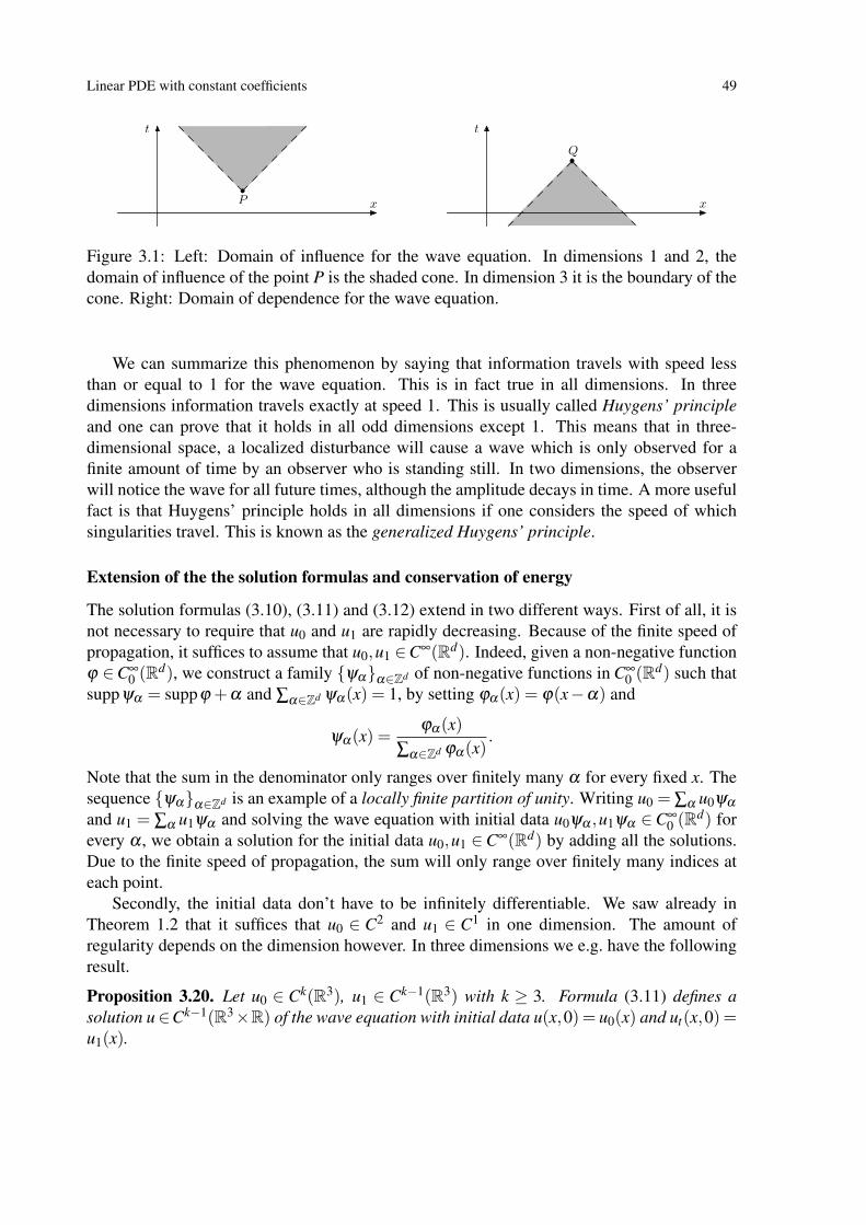
Linear PDE with constant coefficients 49
x
t
P x
t
Q
Figure 3.1: Left: Domain of influence for the wave equation. In dimensions 1 and 2, thedomain of influence of the point P is the shaded cone. In dimension 3 it is the boundary of thecone. Right: Domain of dependence for the wave equation.
We can summarize this phenomenon by saying that information travels with speed lessthan or equal to 1 for the wave equation. This is in fact true in all dimensions. In threedimensions information travels exactly at speed 1. This is usually called Huygens’ principleand one can prove that it holds in all odd dimensions except 1. This means that in three-dimensional space, a localized disturbance will cause a wave which is only observed for afinite amount of time by an observer who is standing still. In two dimensions, the observerwill notice the wave for all future times, although the amplitude decays in time. A more usefulfact is that Huygens’ principle holds in all dimensions if one considers the speed of whichsingularities travel. This is known as the generalized Huygens’ principle.
Extension of the the solution formulas and conservation of energy
The solution formulas (3.10), (3.11) and (3.12) extend in two different ways. First of all, it isnot necessary to require that u0 and u1 are rapidly decreasing. Because of the finite speed ofpropagation, it suffices to assume that u0,u1 ∈C∞(Rd). Indeed, given a non-negative functionϕ ∈C∞
0 (Rd), we construct a family ψαα∈Zd of non-negative functions in C∞0 (Rd) such that
suppψα = suppϕ +α and ∑α∈Zd ψα(x) = 1, by setting ϕα(x) = ϕ(x−α) and
ψα(x) =ϕα(x)
∑α∈Zd ϕα(x).
Note that the sum in the denominator only ranges over finitely many α for every fixed x. Thesequence ψαα∈Zd is an example of a locally finite partition of unity. Writing u0 = ∑α u0ψα
and u1 = ∑α u1ψα and solving the wave equation with initial data u0ψα ,u1ψα ∈C∞0 (Rd) for
every α , we obtain a solution for the initial data u0,u1 ∈C∞(Rd) by adding all the solutions.Due to the finite speed of propagation, the sum will only range over finitely many indices ateach point.
Secondly, the initial data don’t have to be infinitely differentiable. We saw already inTheorem 1.2 that it suffices that u0 ∈ C2 and u1 ∈ C1 in one dimension. The amount ofregularity depends on the dimension however. In three dimensions we e.g. have the followingresult.
Proposition 3.20. Let u0 ∈ Ck(R3), u1 ∈ Ck−1(R3) with k ≥ 3. Formula (3.11) defines asolution u∈Ck−1(R3×R) of the wave equation with initial data u(x,0) = u0(x) and ut(x,0) =u1(x).

50 Linear PDE with constant coefficients
The proof simply relies on changing variables to fix the domain of integration and differ-entiation under the integral sign. The difference with respect to the one-dimensional case hasto do with the fact that the integral in (3.11) is over a two-dimensional surface in R3, whereasthe integral in d’Alembert’s formula is over an open interval in R. One can show that the ‘lossof derivatives’ gets worse the higher the dimension. It is however possible to avoid this byinstead measuring the regularity in terms of Sobolev norms. We will return to this in Chapter5. All of this is in stark contrast to the heat equation, for which initial data which may noteven be continuous evolve into smooth solutions for t > 0 (cf. Proposition 3.9).
Proposition 3.20 only provides an existence result. Uniqueness can be also be proved usingthe energy method.
Theorem 3.21. Let BR(0) be the ball of radius R around the origin in Rd and let Γ = (x, t) ∈Rd×R : |x| ≤ R−|t|. Assume that u ∈C2(Γ) is a solution of the wave equation and that uand ut vanish in BR(0)×0. Then u(x, t)≡ 0 in Γ.
Proof. For simplicity we consider the case t ≥ 0. The other case follows by the change ofvariables t 7→ −t. Since the real and imaginary parts each satisfy the wave equation, we mayalso assume that u is real. Let n(x) = x/(R− t) be the exterior unit normal of the ball BR−t(0)in Rd and dS(x) the surface measure on ∂BR−t(0). Introduce
e(t) =12
∫|x|≤R−t
(u2t + |∇u|2)dx, 0≤ t ≤ R/c.
e′(t) =∫|x|≤R−t
(ututt +∇u ·∇ut)dx− 12
∫|x|=R−t
(u2t + |∇u|2)dS(x)
=∫|x|≤R−t
ut(utt−∆u)dx− 12
∫|x|=R−t
(u2t + |∇u|2−2ut∇u ·n(x))dS(x)
≤ 0,
since u satisfies the wave equation and 2|ut∇u · n(x)| ≤ u2t + |∇u|2. This shows that e(t) is
decreasing. Since e(0) = 0 and e(t)≥ 0 it follows that e(t)≡ 0.
Since the wave equation is linear, this guarantees that any C2 solution is uniquely deter-mined by its initial data. If we assume that ∇u and ut are decaying at infinity and insteadintegrate of Rd , the boundary terms disappear when we integrate by parts. This proves thefollowing result.
Proposition 3.22. Let u0,u1 ∈S (Rd). Then,
E(t) =12
∫Rd(|ut |2 + |∇u|2)dx
is independent of t.
The quantity E can be interpreted as the total energy of the wave. This explains the name‘energy method’ used above. Alternatively, the conservation of energy can be derived by usingthe Fourier representation of the solution. We leave this as an exercises.

Linear PDE with constant coefficients 51
3.3 The Laplace equationLaplace’s equation
∆u = 0
arises e.g. when considering time-independent solutions of the heat or wave equation. Asolution is called a harmonic function. Consider Laplace’s equation in Rd+1. Though oneusually thinks of this as an equation for steady states and not as an evolution equation, wecan of course pick one of the variables, say xd+1, and think of that as our time-variable. Wethus consider Laplace’s equation in the half-space xd+1 > 0 with data given at the hyperplanexd+1 = 0. To emphasize this, we set t = xd+1 and end up with the problem
utt(x, t) =−∆u(x, t), t > 0,u(x,0) = u0(x),ut(x,0) = u1(x).
The corresponding problem on the Fourier side isutt(ξ , t) = |ξ |2u(ξ , t), t > 0,u(ξ ,0) = u0(ξ ),
ut(x,0) = u1(ξ ),
yielding
u(ξ , t) = cosh(t|ξ |)u0(ξ )+sinh(t|ξ |)|ξ |
u1(ξ ).
Here we run into problems since u(·, t) will not even be bounded for t > 0 unless u0 and u1 areexponentially decaying (note that cosh(t|ξ |) and sinh(t|ξ |) grow like et|ξ | at infinity). Thus,there is in general no solution of the form discussed above, unless we assume e.g. that u0 andu1 have compact support. One could of course look for a solution with less regularity, but usingdistribution theory one can in fact show under very mild conditions that there is no solution.There is however the possibility that u0 and u1 fit together in such a way that the exponentiallylarge terms cancel. This will be the case precisely if u1(ξ ) = −|ξ |u0(ξ ). If we are satisfiedwith only prescribing u(x,0) we can therefore find a solution, namely u(ξ , t) = e−t|ξ |u0(ξ ).This gives the solution formula
u(x, t) =1
(2π)d/2
∫Rd
eix·ξ e−t|ξ |u0(ξ )dξ ,
defining a harmonic function in the half plane t > 0. As for the heat equation, it is possible toobtain a solution formula directly in terms of u0 by calculating F−1(e−t|ξ |). The result is
u(x, t) = (Pt ∗u0)(x),
where
Pt(x) =Γ((d +1)/2)
π(d+1)/2t
(t2 + |x|2)(d+1)/2,
is the Poisson kernel for the half-space t > 0, Γ denoting the Gamma function.

52 Linear PDE with constant coefficients
3.4 General PDE and the classification of second order equa-tions
In general, a homogeneous linear second order PDE with real constant coefficients can bewritten
d
∑i, j=1
ai j∂ 2u
∂xi∂x j+
d
∑i=1
ai∂u∂xi
+a0u = 0. (3.13)
The coefficients ai j, ai are real numbers. We assume that not all ai j = 0. Without loss ofgenerality we can assume that ai j = a ji. Consider a linear change of variables y = Bx, whereB is a d×d matrix. That is,
yk = ∑l
bklxl.
Using the chain rule, we obtain that
∂u∂xi
= ∑k
∂u∂yk
∂yk
∂xi= ∑
kbki
∂u∂yk
and∂ 2u
∂xi∂x j=
(∑k
bki∂
∂yk
)(∑
lbl j
∂
∂yl
)u = ∑
k,lbkibl j
∂ 2u∂yk∂yl
.
The second order part of the PDE are therefore converted as follows:
d
∑i, j=1
ai j∂ 2u
∂xi∂x j= ∑
k,l
(∑i, j
bkiai jbl j
)∂ 2u
∂yk∂yl.
We associate to the second order terms the quadratic form
p(ξ ) = ∑i, j
ai jξiξ j = ξT Aξ ,
where ξ ∈ Rd is thought of as a column vector and ξ T is the transpose of ξ . Let q(η) be theform corresponding to the transformed second order part. Then
q(η) = ηT BABT
η .
Note that this is just the change of variables formula associated with the transformation ξ =BT η . Recall that the number of positive (m+) and negative (m−) eigenvalues of the symmetricmatrix associated with a quadratic form is invariant under linear transformations and that wecan find a transformation B so that
q(η) = p(BTη) =
d
∑j=1
σ jη2j ,
in which σ j ∈ −1,0,1 with m+ positive and m− negative squares. We can make a classifi-cation of second order PDE by considering the quadratic form q (or p). The names correspondto the character of the quadratic surface q(η) = c.

Linear PDE with constant coefficients 53
Definition 3.23.
• We say that the PDE (3.13) is elliptic if the quadratic form p is positive or negativedefinite, that is, if all the eigenvalues are positive or if all are negative. In other wordsthis means that after linear change of variables, we can transform the PDE to the Laplaceequation plus terms of lower order.
• If one eigenvalue is positive and the others negative (or vice versa) we say that theequation is hyperbolic. This means that we can transform the equation to the waveequation plus lower order terms.
• If the quadratic form is non-degenerate, but not hyperbolic or elliptic, we say that theequation is ultrahyperbolic. This means that both m+ and m− are ≥ 2 and that d =m++m−. Note in particular that we must have d ≥ 4 for this to be possible.
• Finally, if one eigenvalue is zero and the others have the same sign, we say that theequation is parabolic. Note that this is a degenerate case and that one needs informationon the first order terms to somehow compare the equation with the heat equation.
Roughly speaking, we expect elliptic equations to behave like Laplace’s equation, hyper-bolic equations to like the wave equation and parabolic equations like the heat equation. Alarge portion of the history of PDE has been devoted to finding suitable generalizations ofthese definitions for operators of arbitrary order. Note that this classification by no means isexhaustive, not even for second order equations.
Using multi-index notation, we can write a general linear partial differential operator oforder m with constant coefficients as
∑|α|≤m
aα∂α ,
where aα ∈ C. There is no need to assume that the coefficients are real, but note that acomplex equation always can be written as a system of two real equations. It turns out to bemore convenient to work with the partial derivatives D j = ∂ j/i and D = (∂1, . . . ,∂d)/i. Wetherefore consider operators of the form
P(D) = ∑|α|≤m
aαDα ,
and associate with such an operator the symbol
P(ξ ) = ∑|α|≤m
aαξα
obtained by replacing D j by ξ j. The reason for this choice is that D j corresponds to ξ j on theFourier side, and hence
F (P(D)u)(ξ ) = P(ξ )u(ξ ). (3.14)

54 Linear PDE with constant coefficients
The principal symbol Pm(ξ ) is defined by
Pm(ξ ) = ∑|α|=m
aαξα ,
and the principal part is Pm(D). Just as for second order operators, one can relate propertiesof the PDE to those of the polynomials P and Pm. This is e.g. evident by considering relation(3.14). Our aim will be to find a suitable general definition of hyperbolicity in terms of Pand Pm. The idea is to consider two particular characteristics of the wave equation, namelythe well-posedness of the initial-value problem and the finite speed of propagation. We shalltherefore devote the next section to a study of the initial-value problem for partial differentialoperators with constant coefficients.
For completeness, we also mention the general definition of an elliptic operator.
Definition 3.24 (Ellipticity). We say that the operator P(D) is elliptic if Pm(ξ ) 6= 0 for ξ ∈Rd \0.
Note that this agrees with the definition for second order equations. The idea is essentiallythat one can solve the equation P(D)u = f by dividing with P(ξ ) on the Fourier side. Thisidea doesn’t quite work since P(ξ ) might vanish for small |ξ |. However, ellipticity impliesthat |P(ξ )| ≥ c|ξ |m for large |ξ | and this implies e.g. that u is smooth if f is smooth, since theregularity of u has to do with the decay of u at infinity. The equation
Pm(ξ ) = 0
is called the characteristic equation. We will return to this later on. On the other hand, onecan show that the initial-value problem is always ill-posed in the sense described in Section3.3 for elliptic equations if d ≥ 2. We will not study elliptic operators more in these notessince they’re not directly relevant to waves. Note however that elliptic equations appear in thestudy of special types of waves, such as standing or travelling waves.
3.5 Well-posedness of the Cauchy problemWe consider the Cauchy problem
ut = A(Dx)u, t > 0,u = u0, t = 0.
(3.15)
where A(ξ ) is an n×n matrix with polynomial entries and u is defined on Rd× [0,∞) with val-ues in Rn. Note that scalar equations of order n in t can be reduced to this form by introducingthe time derivatives of order ≤ n−1 as new variables. The corresponding partial differentialoperator is now the matrix-valued operator with symbol
P(ξ ,τ) = iτI−A(ξ ),
where I the unit n×n matrix and we use τ to denote the Fourier variable corresponding to t.
Linear PDE with constant coefficients 55
Example 3.25. The wave equation utt = ∆u can be writtenut = v,vt = ∆u,
which is of the above form with
A(ξ ) =(
0 1−|ξ |2 0
).
Definition 3.26 (Well-posedness in the sense of Hadamard). We say that the Cauchy problemis well-posed if:
(1) there exists a solution for each u0;
(2) the solution is unique;
(3) the solution depends continuously on the data u0.
Of course, this has to be made more precise in the sense that one has to specify the class ofinitial data, the class of solutions and the topology used to measure the continuity of the mapu0 7→ u. We will consider data u0 ∈S (Rd)n, meaning that each component of u0 belongs toS (Rd). Note that Definition 3.1 extends in a natural way to functions with values in S (Rd)n
by imposing the conditions on each component.
Definition 3.27. The Cauchy problem (3.15) is said to be well-posed in S if
(1) for every u0 ∈S (Rd)n there exists a unique solution
u = S(·)u0 ∈C∞([0,∞);S (Rd)n);
(2) the map S : S (Rd)n→C∞([0,∞);S (Rd)n), S(t)u0 = u(t), is continuous.
If the Cauchy problem is not well-posed it is said to be ill-posed (in S ).
Remark 3.28. The assumption that u ∈ C∞([0,∞);S (Rd)n) in the uniqueness result can berelaxed. It suffices e.g. to assume that u ∈C([0,∞);S (Rd)n)∩C1((0,∞);S (Rd)n). From theequation ut = A(Dx)u it is then easy to prove that u∈C2((0,∞);S (Rd)n) with ∂tut = A(Dx)utand ut(0) = A(Dx)u0. Using induction, we find that u ∈C∞((0,∞);S (Rd)n). Moreover, allthe derivatives extend continuously to t = 0.
We look for a general condition under which the initial-value problem is well-posed in S .Taking the Fourier transform of (3.15) we obtain the problem
ut = A(ξ )u, t > 0,u = u0, t = 0.
(3.16)

56 Linear PDE with constant coefficients
Note that (3.16) is a linear system of ordinary differential equations. We therefore know thatfor each ξ and u0(ξ ), (3.16) has a unique solution
u(ξ , t) = etA(ξ )u0(ξ ).
Moreover, since A(ξ ) is a polynomial in ξ , u ∈C∞(Rd× (0,∞))n. In order for u(·, t) to be ofSchwartz class, we need to control the growth of etA(ξ )u0(ξ ) for large ξ . The idea is that thiscan be done by prescribing a condition on the eigenvalues of A.
Definition 3.29 (Petrowsky’s condition). We say that A(Dx) satisfies Petrowsky’s condition ifthere exists a number CA ∈R such that the eigenvalues λ (ξ ) of A(ξ ) satisfy Reλ (ξ )≤CA forall ξ ∈ Rd .
Remark 3.30.
(1) Consider the symbol P(ξ ,τ) = iτI−A(ξ ) of the operator ∂tI−A(Dx). An equivalentformulation of Petrowsky’s condition is that detP(ξ ,τ) 6= 0 if Imτ ≤−CA.
(2) Petrowsky’s original condition was in fact a logarithmic bound on Reλ (ξ ). It wasshown by Gårding in the special case of hyperbolic operators that this condition isequivalent to the one in the definition. The equivalence in general follows from theTarski-Seidenberg theorem discussed below. This was first observed by Hörmander.
Theorem 3.31. The Cauchy problem (3.15) is well-posed in S if A(Dx) satisfies Petrowsky’scondition.
To clarify the proof, we first treat the scalar case n = 1. A(ξ ) = a(ξ ) is then a complexnumber for each ξ and the condition means that Rea(ξ )≤CA for all ξ ∈ Rd . It follows that
|eta(ξ )|= et Rea(ξ ) ≤ eCat , t ≥ 0.
Henceu(ξ , t) = eta(ξ )u0(ξ ) ∈S (Rd)
for each t ≥ 0. A familiar argument shows that
u(x, t) =1
(2π)d/2
∫Rd
eix·ξ eta(ξ )u0(ξ )dξ ,
defines a solution of the equation. A straight-forward proof shows that the function t 7→ u(·, t)satisfies the conditions of Definition 3.27.
For the general case one needs a property of the matrix exponential. This property is bestproved using complex analysis.
Lemma 3.32. There exists a constant C > 0 such that
‖eA‖ ≤C(1+‖A‖n−1)emaxReσ(A)
for A ∈ Cn×n, where σ(A) denotes the spectrum (set of eigenvalues) of A and ‖ · ‖ denotes thematrix norm.

Linear PDE with constant coefficients 57
Proof. The proof relies on the following representation of the matrix exponential:
etA =1
2πi
∮|z|=r
etz(zI−A)−1 dz, (3.17)
where r is chosen so that all the eigenvalues of A are contained in the ball Br(0)= z∈C : |z|<r and the contour is traversed counterclockwise. The path integral of a matrix-valued functionis just the matrix formed by taking the path integral of each element of he matrix.
To prove formula (3.17), let B(t) be the function defined by the path integral. Notice firstthat the function z 7→ etz(zI−A)−1 is analytic away from the eigenvalues of A (again definedby considering each element). It follows that B(t) is independent of r. By the properties of thematrix exponential, it suffices to check that
B′(t) = AB(t)
and B(0) = I. Using the identity
(zI−A)−1 = z−1(I +A(zI−A)−1),
and Cauchy’s theorem, we find that
B(0) =1
2πi
∮|z|=r
(zI−A)−1 dz
=1
2πi
∮|z|=r
z−1(I +A(zI−A)−1)dz
= I +1
2πi
∮|z|=r
z−1A(zI−A)−1 dz.
Recall now Cramer’s rule, which says that
A−1j,k = (−1) j+k detAk, j
detA,
where Ak, j is the matrix obtained if one removes row number k and column number j from A.From this it follows that ‖(zI−A)−1‖ ≤C|z|−1 as |z| → ∞. Consequently,∥∥∥∥ 1
2πi
∮|z|=r
z−1A(zI−A)−1 dz∥∥∥∥≤ C
r→ 0
as r→ ∞, so that B(0) = I. Finally, we have that
B′(t)−AB(t) =1
2πi
∮|z|=r
etzI dz = 0.
This proves formula (3.17).
Define now a path Γ in C as follows. Let λ j, j = 1, . . . ,k be the distinct eigenvalues of A,in order of increasing real part. For each j, let B1(λ j) be the open disc of radius 1 around λ j.

58 Linear PDE with constant coefficients
Form the union U = ∪kj=1B1(λ j(A)) (note that some of the discs may intersect). Let Γ be the
boundary of U , traversed counterclockwise. Deforming the contour |z| = r into Γ, we obtainfrom (3.17) that
eA =1
2πi
∮Γ
ez(zI−A)−1 dz.
On Γ we have that |z−λ j| ≥ 1 for each j. Writing,
det(zI−A) = Πkj=1(z−λ j)
m j ,
where m j is the algebraic multiplicity of λ j, it follows that
|det(zI−A)| ≥ 1.
Using Cramer’s rule, we find that
(zI−A)−1j,k = (−1) j+k det((zI−A)k, j)
det(zI−A)−1 ,
where det((zI−A)k, j) is a polynomial of degree at most n− 1 in z, the coefficients of whichare products of the elements of A. We can therefore estimate
‖(zI−A)−1‖ ≤C1(|z|n−1 +‖A‖n−1).
On the other hand, when z belongs to Γ it follows that |z− λ j| = 1 for some j. Using thetrivial estimate |λ j| ≤ ‖A‖, which follows from the definition of an eigenvalue, we find that|z| ≤ ‖A‖+1 on Γ. We conclude that ‖(zI−A)−1‖ ≤C2(1+‖A‖n−1). Finally, |ez|= eRez ≤eReλk+1 on Γ and the total length of Γ is at most 2πn. It follows that
‖eA‖ ≤∥∥∥∥ 1
2πi
∮Γ
ez(zI−A)−1 dz∥∥∥∥≤C(1+‖A‖n−1)eReλk ,
where C = nC2e.
Proof of Theorem 3.31. Given the assumptions in the theorem and the previous lemma it isnot difficult to see that
‖etA(ξ )‖ ≤C(1+ |t|n−1|ξ |m)eCAt ,
where m is the maximum degree of the elements of A(ξ ) times n−1. We therefore find that
‖ξ α u(ξ , t)‖L∞(Rd) ≤C ∑|β |≤|α|+m
‖ξ β u0(ξ )‖L∞(Rd)
uniformly for t in a compact interval, for some other constant C. The solution of a system ofordinary differential equations whose coefficients are C∞ functions of some parameter dependssmoothly on that parameter. It follows that u is C∞. Differentiating (3.16) with respect to ξk,we find that
∂ξkut = A(ξ )∂ξk
u+(∂ξkA(ξ ))u, t > 0,
∂ξku = ∂ξk
u0, t = 0,

Linear PDE with constant coefficients 59
and hence∂ξk
u(ξ , t) = etA(ξ )∂ξk
u0(ξ )+∫ t
0e(t−s)A(ξ )(∂ξk
A(ξ ))u(t,ξ )dξ .
We also have that∂t u(ξ , t) = etA(ξ )A(ξ )u0(ξ ).
This will at most increase |u(ξ , t)| by a polynomial factor. The same holds whenever we takea finite number of derivatives. Since u0 ∈ S , we therefore find that u(·, t) ∈ S and henceu(·, t) ∈S .
To prove that t 7→ u(·, t) is continuous we use the formula
u(x, t) = (2π)−d/2∫Rd
eix·ξ etA(ξ )u0(ξ )dξ .
It follows that
‖u(·, t +h)−u(·, t)‖L∞(Rd) ≤C∫Rd‖e(t+h)A(ξ )− etA(ξ )‖|u0(ξ )|dξ .
For any ε we can choose R so large that∫|ξ |≥R
‖e(t+h)A(ξ )− etA(ξ )‖|u0(ξ )|dξ ≤C∫|ξ |≥R
(1+ |ξ |m)|u0(ξ )|dξ ≤ ε,
while ∫|ξ |≤R
‖e(t+h)A(ξ )− etA(ξ )‖|u0(ξ )|dξ ≤Ch∫|ξ |≤R
|u0(ξ )|dξ → 0
as h→ 0. It follows that ‖u(·, t +h)−u(·, t)‖L∞(Rd)→ 0 as h→ 0. Similar estimates are easilyobtained for all the other semi-norms. To prove that u is C1 in t one needs in addition theidentity
e(t+h)A(ξ )− etA(ξ ) =∫ t+h
tA(ξ )esA(ξ ) ds,
from which it follows that∥∥∥∥∥e(t+h)A(ξ )− etA(ξ )
h
∥∥∥∥∥= (1+ |ξ |m′)e(t+h)CA,
for some m′. Splitting the integral as above it then follows that ‖u(·,t+h)−u(·,t)h −ut(·, t)‖α,β → 0
as h→ 0 for every semi-norm, where ut is the formal time-derivative of u,
ut(x, t) = (2π)−d/2∫Rd
eix·ξ A(ξ )etA(ξ )u0(ξ )dξ .
The continuity of ut is shown as above. It follows that t 7→ u(·, t) belongs to C1([0,∞);S (Rd))and hence to C∞([0,∞);S (Rd)) using the equation (see Remark 3.28). The continuity of themap u0 7→ u follows from the estimates
‖u(·, t)‖α,β ≤C ∑|β ′|≤|β |+m
‖u0‖α,β ′
and the linearity of the equation (again using Remark 3.28).

60 Linear PDE with constant coefficients
One can show that Petrowsky’s condition is also necessary for well-posedness in S . Forthis it is necessary to use a result from algebraic geometry known as the Tarski-Seidenbergtheorem. This result implies that the maximum real part of the eigenvalues of A(ξ ) either isbounded or grows as a power in |ξ | as ξ → ∞. More precisely, one has that
maxReλ : det(λ I−A(ξ )) = 0 for some ξ ∈ Rd with |ξ |= r= crα(1+o(1))
as r→ ∞ for some α ∈Q and c ∈ R. Suppose that Petrowsky’s condition is violated. We canthen find a sequence ξ j→ ∞ and corresponding eigenvalues λ j with Reλ j ∼ c|ξ j|α , c,α > 0.Let e j be a sequence of corresponding unit eigenvectors. Choosing
u j(ξ ) = |ξ j|−1ϕ(ξ −ξ j)e j,
for some fixed function ϕ ∈C∞0 (Rd) with ϕ(0) = 1, we obtain that
|etA(ξ j)u j(ξ j)|= |ξ j|−1e(Reλ j)te j ∼ |ξ j|−1ec|ξ j|α te j,
so that u j(·, t) = F−1(u j(·, t)) is ubounded in S (Rd) for any fixed t > 0, while u0, j =F−1(u j)→ 0 in S (Rd). This proves that (2) in Definition 3.27 is violated. In fact, onecan show that for ‘most’ initial data, there is not even a solution in the sense of Definition3.27.
Example 3.33. Consider the scalar equation ut = a(Dx)u, where
a(ξ ) = amξm,
with am 6= 0. To avoid trivialities, we suppose that m ≥ 1. If m is odd, the equation is well-posed if and only if am is purely imaginary. If m is even, the equation is well-posed if and onlyif Ream ≤ 0.
Example 3.34. The linearized KdV equation ut + uxxx = 0 can be written ut = a(Dx)u witha(ξ ) = iξ 3. Thus, it is well-posed. So is the Schrödinger equation iut +uxx = 0, which can bewritten ut = a(Dx)u with a(ξ ) =−iξ 2.
Example 3.35. The heat equation ut = ∆u can be written ut = a(Dx)u with a(ξ ) = −|ξ |2.Thus, it is well-posed. However, the backwards heat equation ut = −∆u is ill-posed. Thisequation is obtained by considering the evolution of the heat equation for t < 0.
Since we have assumed that A(Dx) is independent of t, the semigroup property follows atonce if Petrowsky’s condition is satisfied. On the Fourier side this corresponds to the identity
e(s+t)A(ξ ) = esA(ξ )etA(ξ ).
One sometimes uses the notationS(t) = etA(Dx)
due to the similarity with the matrix exponential.
Finally, we consider the inhomogeneous problemut = A(Dx)u+ f , t > 0,u = u0, t = 0,
(3.18)
which will play a big role when we consider nonlinear equations.

Linear PDE with constant coefficients 61
Theorem 3.36 (Duhamel’s formula). Let f ∈ C∞([0,∞);S (Rd)) and u0 ∈ S (Rd) and as-sume that A satisfies Petrowsky’s condition. The inhomogeneous Cauchy problem (3.18) hasa unique solution u ∈C∞([0,∞);S (Rd)) given by
u(t) = etA(Dx)u0 +∫ t
0e(t−s)A(Dx) f (s)ds, t ≥ 0.
The solution formula should be interpreted pointwise for each x ∈ Rd .
Proof. Working on the Fourier side, we find that any solution must satisfy
u(ξ , t) = etA(ξ )u0(ξ )+∫ t
0e(t−s)A(ξ ) f (ξ ,s)ds, t ≥ 0
from the theory of ordinary differential equations. On the other hand, u(ξ , t) defined by thisformula is a solution of the the transformed version of the problem. Using the same approachas in the proof of Theorem 3.31 one shows that e(t−s)A(ξ ) f (ξ ,s) is a smooth function of s andt with values in S (Rd) when 0 ≤ s ≤ t. It is then an easy matter to prove that u belongs toC∞([0,∞);S (Rd)). It follows from Lemma 3.2 that the same is true for u = F−1(u). Since(ξ ,s) 7→ e(t−s)A(ξ ) f (ξ ) is in L1(Rd× [0, t]) we can change the order of integration to deducethat
F−1(∫ t
0e(t−s)A(ξ ) f (ξ ,s)ds
)=∫ t
0F−1(e(t−s)A(ξ ) f (ξ ,s))ds =
∫ t
0e(t−s)A(Dx) f (s)ds.
3.6 Hyperbolic operatorsAs mentioned in Section 3.4, hyperbolic operators are those for which the Cauchy problemis well-posed and which have the property of finite speed of propagation. By finite speedof propagation we mean that the solution u(x, t) has compact support for a fixed t if u0 hascompact support. One can show that a necessary and sufficient condition for this to hold isthat
det(λ I−A(ξ )) has degree at most n in ξ . (3.19)
The idea is that if u(x, t) has compact support, then its Fourier transform
u(ξ , t) = (2π)−d/2∫
suppu(·,t)u(x, t)e−ix·ξ dx
can be extended to the whole complex plane. Moreover, we have an estimate of the form
|u(ξ , t)| ≤CeK| Imξ |, ξ ∈ C. (3.20)
On the other hand, we know that u(ξ , t) = etA(ξ )u0(ξ ) and one can show that this together with(3.20) implies a growth condition of the form |λ (ξ )| ≤C(1+ |ξ |) on the eigenvalues of A(ξ ).This leads to the condition (3.19). For the converse, one needs a characterization of functionsof compact support in terms of their Fourier transform. One can show that if u(·, t) is an entire

62 Linear PDE with constant coefficients
analytic function satisfying (3.20), then u(·, t) has compact support. Results of this type arecalled Paley-Wiener theorems. A proof of these facts is beyond the scope of these notes.
An equation which is well-posed in S (Rd) and has finite speed of propagation is in factwell-posed in C∞ (see the discussion before Proposition 3.20). The hypothesis of finite speedof propagation is crucial for this to hold. It can be shown that if the condition (3.19) is violated,there exists a non-zero solution u ∈C∞(Rd ×R) of ut = A(Dx)u which vanishes in the half-space t ≤ 1. Thus, uniqueness is lost for the Cauchy problem.
We are now ready for the definition of a hyperbolic operator with constant coefficients. Theoperator ∂tI−A(Dx) is said to be hyperbolic if it satisfies condition (3.19) and Petrowsky’scondition (Definition 3.29). For a general partial differential operator P(D) in Rd , it maynot be clear what to consider as the time-variable. Moreover, one may also wish to solvethe Cauchy problem with data on a hypersurface in Rd . It is therefore useful to have a moregeneral definition of hyperbolicity.
Definition 3.37 (Hyperbolicity).
(1) A scalar partial differential operator P(D) of order m is said to be hyperbolic in thedirection ν ∈ Rd if its principal part satisfies
Pm(ν) 6= 0,
and there exists τ0 ∈ R such that
P(ξ + τν) 6= 0, ξ ∈ Rd, Imτ ≤ τ0.
(2) P(D) is said to be strictly hyperbolic in the direction ν if, in addition, for every ξ ∈ Rd
not parallel with ν , the equation
Pm(ξ + τν) = 0,
has only simple real roots τ .
(3) A matrix-valued operator P(D) is said to be (strictly) hyperbolic if detP(D) is (strictly)hyperbolic.
Note that we recover the definition of hyperbolicity for P(D) = ∂tI − A(Dx) by takingν = (0,1) ∈ Rd×R.
In the following discussion we consider a scalar operator P(D). The condition Pm(ν) 6= 0is the analogue of (3.19). We say that the direction ν is non-characteristic for P if this condi-tion holds. A smooth (d−1)-dimensional hypersurface Σ in Rd is said to be non-characteristicif at each point of Σ, the normal is a non-characteristic direction for P. The Cauchy problemwith data on Σ consists of prescribing the values of the function u and all normal derivativesof u of order strictly less than m on Σ. One can show that the Cauchy problem for a hyperbolicoperator with C∞ data on a non-characteristic hypersurface is well-posed. If one only assumes

Linear PDE with constant coefficients 63
that the surface is non-characteristic, one can still prove the (local) existence and uniquenessof solutions with real-analytic data if Σ is real-analytic. This is the Cauchy-Kovalevskaya the-orem. Intuitively, the assumption means that the normal derivative of order m can be expressedin terms of the normal derivatives of order ≤ (m− 1) (the data) and their tangential deriva-tives. This can be used to construct a formal power series solution, and the proof consistsof showing that the series converges. In fact, the theorem also holds for nonlinear equations.The assumption of real-analyticity is often too strong for the theorem to be of any practicalrelevance. Moreover, the solution may not depend continuously on the data.
Let us briefly mention something about operators
P(x,D) = ∑|α|≤m
aα(x)Dα ,
with (smooth) variable coefficients. We say that P is (strictly) hyperbolic in the direction ν
at x0 if P(x0,D) is (strictly) hyperbolic in the direction ν . It turns out that strict hyperbolicityis sufficient for well-posedness, whereas the weaker notion is not. However, there are certainnotions in between which are useful. Consider e.g. the first order system
A0(x, t)∂tu−d
∑k=1
Ak(x, t)∂ku−B(x, t)u = 0, (3.21)
where u = (u1, . . . ,un) ∈ Rn, and B and Ak, k = 0, . . . ,d, are n×n real matrices.
Definition 3.38. The system (3.21) is called a symmetric hyperbolic system if all the matricesAk(x, t) are symmetric and A0(x, t) is positive definite for all (x, t).
One can prove that the Cauchy problem with initial data on t = 0 is well-posed also forsuch systems.

64 Linear PDE with constant coefficients

Chapter 4
First order quasilinear equations
After our study of linear equations in the previous chapter, we now turn to nonlinear hyper-bolic equations. We will focus on real first order equations since these can be solved by themethod of characteristics. The main emphasis is on showing that initially smooth solutionscan develop singularities. This is something one encounters already in a course on ordinarydifferential equations, where solutions of the nonlinear equation x = x2 blow up in finite time.We will also briefly discuss how one can continue a solution after the development of a sin-gularity. To do this we introduce the concept of weak solutions. Since weak solutions are ingeneral not differentiable, they cannot satisfy the PDE in the classical sense. To interpret thesolution one has to go back to the original physical problem. We will do this for a class ofequations called conservation laws, for which weak solutions have a natural interpretation.
More details on the method of characteristics can be found in Evans [7] or John [14]. Formore on hyperbolic conservation laws, see e.g. Bressan [4], Hörmander [11], Holden andRisebro [10] and Lax [17].
4.1 Some definitions
A general partial differential equation of order m can be written
F(x,∂ αu(x); |α| ≤ m) = 0, x ∈Ω, (4.1)
where Ω⊂ Rd and the notation means that the real-valued function F depends on u and all ofits derivatives of order less than or equal to m. Note that we now assume that u is real-valued.This will be the case throughout the entire chapter. In the previous chapter we discussed linearPDE,
∑|α|≤m
aα(x)∂ αu(x) = f (x), x ∈Ω,
for given functions aα , f : Ω→ R. We mostly discussed the homogeneous case f = 0. Non-linear equations are divided into different classes depending on ‘how nonlinear’ they are.
65

66 First order quasilinear equations
Definition 4.1.
(1) A PDE is said to be semilinear if it has the form
∑|α|=m
aα(x)∂ αu+b(x,∂ β u; |β | ≤ m−1) = 0. (4.2)
(2) It is said to be quasilinear if it has the form
∑|α|=m
aα(x,∂ β u; |β | ≤ m−1)∂ αu+b(x,∂ β u; |β | ≤ m−1) = 0. (4.3)
(3) It is said to be fully nonlinear if it depends nonlinearly on the highest derivatives.
In other words, the highest derivatives appear linearly in a quasilinear equation. If thecoefficients of the highest derivatives are also independent of the function u and its derivatives,the equation is semilinear. A rule of thumb is that a PDE is more difficult to handle the morethe nonlinearity affects the highest derivatives.
Example 4.2.
• The KdV equationut +uux +uxxx = 0
is an example of a semilinear equation. So is the nonlinear wave equation
utt−∆u+ f (u) = 0,
where f : R→ R is a given function.
• Burgers’ equationut +uux = 0
is an example of a quasilinear equation, which is not semilinear.
• An important example of a fully nonlinear equation is obtained as follows. Consider ahypersurface Σ in Rd×R, given implicitly by S(x, t) = 0, where S is a C1-function. Σ ischaracteristic for the wave equation utt =∆u if the normal is a characteristic direction forthe wave equation at each point of Σ. Since the normal at (x, t) is given by ∇(x,t)S(x, t),this condition can be written
S2t −|∇S|2 = 0.
This is the eikonal1 equation. Assuming that S(x, t) = t−u(x), the eikonal equation issometimes rewritten
|∇u|2 = 1.
1From the Greek word for image.
First order quasilinear equations 67
One can define characteristic directions and hyperbolicity also for nonlinear equations. Fora semilinear eqution it is natural to define ξ ∈ Rd to be a characteristic direction at the pointx ∈ Ω if ξ is a characteristic direction of the linear operator ∑|α|=m aα(x)∂ α . The definitionis similar in the quasilinear case: ξ ∈ Rd is a characteristic direction if ξ is characteristicfor ∑|α|=m aα(x,u(x), . . . ,∂ m−1u(x))∂ α . This condition depends on both x and the function u.Strict hyperbolicity is defined in an analogous manner. In the fully nonlinear case, one candefine strict hyperbolicity in terms of the linearization at u. The linearization at u is obtainedby calculating
ddε
F(x,∂ α(u+ εv))∣∣∣ε=0
= ∑|α|≤m
aα(x)∂ αv(x),
where
aα(x) =∂F
∂ (∂ αu)(x,∂ β u(x)).
We say that the equation (4.1) is strictly hyperbolic if its linearization is strictly hyperbolic.We leave it as an exercise to prove that this agrees with the previous definitions in the case thatthe equation is semilinear or quasilinear.
Example 4.3. Consider the first order quasilinear equation
a1(x,u)∂1u+ · · ·+ad(x,u)∂du = f (x,u)
in Rd . The direction ν ∈ Rd is non-characteristic at x and u if
a(x,u) ·ν 6= 0,
where a(x,u) = (a1(x,u), . . . ,ad(x,u)). The equation is then automatically strictly hyperbolic,since the equation
a(x,u) · (ξ + τν) = 0
has the real root τ = −(a(x,u) · ξ )/(a(x,u) · ν) for each ξ ∈ Rd . The equation also sharesthe finite speed of propagation property with the linear hyperbolic equations with constantcoefficients discussed in the previous chapter. This follows from the method of characteristicsdiscussed below.
Many of the models which appear in physics are in fact systems of PDE. The only differ-ence is that u and F are then vector valued. One usually assumes that the number of equationsequals the number of unknown functions. One can make a similar division into linear, semi-linear, quasilinear and fully nonlinear equations.
4.2 The method of characteristicsWe consider now first order quasilinear equations
a1(x,u)∂1u+ · · ·+ad(x,u)∂du = f (x,u). (4.4)
68 First order quasilinear equations
The coefficients a j are assumed to be C1 functions. Our goal is to solve (4.4) by turning it intoan appropriate system of ODE. Given u, we can define a curve x : I→Rd , I = (s0,s1)⊂R, byx(s) = a(x(s),u(x(s))). The left hand side of (4.4) is the derivative of u along the curve x(s).In other words, z(s) = f (x(s),z(s)), where z(s) = u(x(s)). This closes the system and we haveobtained the characteristic equations
x(s) = a(x(s),z(s)),z(s) = f (x(s),z(s)).
(4.5)
The curves x(s) are called characteristics, although this name is sometimes used for the curves(x(s),z(s)) in Rd+1. If equation (4.4) is semilinear, the first equation doesn’t involve z(s). Wecan then first find the characteristic x(s) and then solve the second equation. If the originalequation is linear this simply entails integrating f (x(s)).
Example 4.4. Consider the linear equation x1∂2u− x2∂1u = f (x) in R2. The characteristicequations are
x1(s) =−x2(s),x2(s) = x1(s).z(s) = f (x(s)).
The characteristics are circles, x(s) = r(coss,sins), r > 0 fixed. Once we know this, we obtainthat
u(r coss,r sins) =∫ s
0f (r cosθ ,r sinθ)dθ +g(r),
where g is arbitrary. Note that a necessary condition in order to obtain a global solution is that∫ 2π
0f (r cosθ ,r sinθ)dθ = 0
for every r, since otherwise we will not obtain the same value of u when we go one timearound the origin.
We now illustrate how the characteristics can be used to solve the Cauchy problem in theneighbourhood of a point. For simplicity we assume that the initial data u0 is given on thehyperplane xd = 0.
Theorem 4.5 (Local solvability). Let u0 ∈C1(U) for some open set U ⊂Rd−1 and let y0 ∈U.Assume that moreover that a and f are C1 in Rd and that the equation is non-characteristic inthe direction ed at (y0,0) and u0. There exists an open subset W ⊂Rd with W ∩(Rd−1×0)⊂U such that equation (4.4) has unique solution u ∈C1(W ) with u(y,0) = u0(y).
Proof. The solution is obtained by solving the characteristic equations (4.5) with initial datax(0;y) = (y,0) and z(0;y) = u0(y), where y ∈U . By the theory of ordinary differential equa-tions, there exists for each y a maximal solution x(s;y) defined for s in some open inter-val I(y) containing the origin. Moreover, the function (y,s) 7→ x(s;y) is C1 on the open set

First order quasilinear equations 69
∪y∈Uy× I(y). We wish to define the solution for s 6= 0 as u(x(s;y)) = z(s;y). This re-quires that the map y 7→ x(s;y) is injective, in other words, that the characteristics don’t cross.Moreover, as y and s vary, the curves x(s;y) should trace out an open set W ⊂ Rd . Both ofthese conditions follow from the inverse function theorem if we can prove that the Jacobianof the map (y,s) 7→ x(s;y) is non-zero at s = 0 and y = y0. Since x(0;y) = (y,0) it follows that∂y jxi(0;y) = δi j. We also have that ∂sx(0;y) = a((y,0),u0(y)) from (4.5). Hence, the Jacobianis ∣∣∣∣∣∣∣∣∣
1 0 . . . a1((y0,0),u0(y0))0 1 . . . a2((y0,0),u0(y0))...
... . . . ...0 0 · · · ad((y0,0),u0(y0))
∣∣∣∣∣∣∣∣∣= ad((y0,0),u0(y0)) 6= 0
by the non-characteristic assumption. The fact that u defined in this way is a solution of theproblem follows from the inverse function theorem and the definition of the characteristics.The uniqueness of the solution follows from the construction.
For details on the generalization of the method of characteristics to fully nonlinear firstorder equations and the solution of the Cauchy problem with data on a noncharacteristic hy-persurface in Rd we refer to Evans [7, Chapter 3.2].
4.3 Conservation laws
We used the conservation of energy in the derivation of the heat equation in Section 3.1.1.Suppose more generally that we have a time-dependent real-valued function u on Rd whichdescribes the ‘density’ of some quantity, e.g. the concentration of some substance in a fluid.The total amount of substance in the region Ω⊂ Rd is then given by∫
Ω
u(x, t)dx.
Assume that the production of the substance at a point (x, t) in space and time is given byg(x, t) (substance is destroyed if g(x, t)< 0) and that the flow of the substance is described bythe vector-valued function f : Rd×R→Rd . The same considerations as in Section 3.1.1 leadto the equation
ddt
∫Ω
u(x, t)dx =−∫
∂Ω
f (x, t) ·ndS+∫
Ω
g(x, t).
Assuming again that all the involved functions are continuous, we obtain the continuity equa-tion
ut +∇ · f = g.
To get any further one has to know the form of f and g, which depends on the specific problem.In many cases, f and g depend on u and possibly its derivatives. The relation between thesequantities is called a constitutive law. We shall assume throughout the rest of the chapter that

70 First order quasilinear equations
f (x, t) = f (u(x, t)), that is, f depends solely on u. We will also mostly consider the case g≡ 0.The equation of interest is therefore
ut +∇ · f (u) = 0.
This is called a scalar conservation law. The function f is sometimes called the flux functionin this context. Carrying out the differentiation, we find that
ut +a1(u)∂1u+ · · ·+ad(u)∂du = 0,
where ai(u) = f ′i (u), i = 1, . . . ,d. In particular, we notice that a scalar conservation law alwaysis hyperbolic in the t-direction (cf. Example 4.3). Many of the interesting problems fromphysics are in fact systems of conservation laws.
∂tu j +∇ · f j(u) = 0, (4.6)
where u = (u1, . . . ,un) : Rd → Rn and f j : Rn→ Rd , j = 1, . . . ,n.
Example 4.6 (Burgers’ equation). Burgers’ equation ut +uux = 0 can be rewritten as the scalarone-dimensional conservation law
ut +
(u2
2
)x= 0
with flux f (u) = u2/2.
Example 4.7 (Equations of gas dynamics). The macroscopic description of a gas (or any otherfluid) involves the fluid velocity u, the density ρ , the pressure p and the energy E. The first is avector quantity while the others are scalar quantities. At a given moment in time, the functionsare defined in some open subset of R3. The flow of substance across a surface is given by ρu ·n,where n is the unit normal. The conservation of mass can therefore be expressed in the form
ρt +∇ · (ρu) = 0. (4.7)
Basic principles of physics require balance of momentum. This is expressed as the conserva-tion law2
∂t(ρu j)+∇ · (ρu ju)+∂ j p = ρFj, (4.8)
where ρu j are the components of the momentum density, ρu ju · n the components of themomentum flow across a surface, p is the pressure and Fj the components of the body forces(e.g. gravity). Here we have neglected viscosity. Equation (4.8) can be written in vectornotation as
∂t(ρu)+∇ · (ρu⊗u)+∇p = ρF,
2We’re abusing the terminology here, since the equations are not of the form (4.6). Introducing new variablesw j = ρu j we would however obtain (4.6) with source terms.

First order quasilinear equations 71
where u⊗u=(u juk) j,k ∈Rd is the outer product of the the vector u with itself. In addition, oneneeds an equation for the conservation of energy. Ignoring heat conduction and production,this takes the form
∂tE +∇ · (u(E + p)) = ρF ·u, (4.9)
where E is the total energy per unit volume. E is the sum of internal energy and kineticenergy associated with the macroscopic motion, E = ρe+ 1
2ρ|u|2, where e denotes the specificinternal energy (internal energy per unit mass). In general one should add a a heat flux termas in Section 3.1.1 and possibly a heat production term. The considerations so far are notspecific for gases, and would work equally well for a liquid. Note that we have six unknowns(counting all components of u) but only five equations (4.7)–(4.9). This means that we have anunderdetermined system. Liquids are assumed to be incompressible, mathematically meaningthat introduces the extra equation ∇ ·u. For a gas one adds instead a constitutive relation of theform e = e(p,ρ). Assuming that we are dealing with an ideal gas with constant entropy (anisentropic gas) the equations can be reduced to (4.7)–(4.8) together with a constitutive relation
p = f (ρ),
where f (ρ) = κργ for some constants κ > 0 and γ > 1. Here we have also assumed that thegas is polytropic, that is, that it has constant specific heat capacities. Equation (4.8) can besimplified using (4.7). Carrying out the differentiation in (4.8), one obtains that
(ρt +∇ · (ρu))u j +ρ(∂tu j +u ·∇u j
)+∂ j p = ρFj,
which simplifies to
ut +(u ·∇)u+1ρ
∇p = F (4.10)
due to the identity (4.7). Equation (4.10) is the usual form of Euler’s equations. Note that(4.8) can be written in the similar form
ρt +u ·∇ρ +ρ∇ ·u = 0.
The differential operatorDDt
= ∂t +u ·∇,
called the material derivative, has a very natural interpretation. Suppose that we follow a verysmall parcel of gas. The parcel is approximated by a single mass at the point x(t) (a ‘fluidparticle’). The evolution of this particle is governed by the equation
x(t) = u(x(t), t).
The material derivative of some physical quantity, such as the density, is then simply thederivative of the quantity along the path of a fluid particle, that is,
ddt
ρ(x(t), t)
= ρt(x(t), t)+u(x(t), t) ·∇ρ(x(t), t) =
Dρ
Dt(x(t), t).
See Whitham [28, Chapter 6] for a much more extensive discussion of gas dynamics.

72 First order quasilinear equations
Example 4.8 (The linearized equations of gas dynamics). We now show how the linearizedequations of gas dynamics discussed in Example 1.1 can be derived from (4.7) and (4.10)under the assumption (4.7). We assume in addition that there are no external forces (F = 0).Note that a constant state u ≡ 0, ρ ≡ ρ0 and p ≡ p0 := f (ρ0) is a solution of the equations.Consider now a small perturbation of the constant state: ρ = ρ0+ερ and u = ε u, where ε is asmall parameter. Substituting this into the governing equations, expanding in powers of ε anddividing by ε , we obtain
ρt +ρ0∇ · u = O(ε)
and
ut +f ′(ρ0)
ρ0∇ρ = O(ε).
Neglecting terms of order ε and dropping the tildes for notational convenience, we arrive atthe linearized equations
ρ0ut + c20∇ρ = 0,
ρt +ρ0∇ ·u = 0,
from Example 1.1, where c0 =√
f ′(ρ0).
Example 4.9 (Traffic model). We discuss a simple model for traffic flow introduced inde-pendently by Lighthill and Whitham [18] and Richards [21]. Consider a road consisting of asingle lane. The traffic is described by a the density ρ(x, t) of cars per unit length. The numberof cars in the stretch [a,b] is given by
∫ ba ρ(x, t)dx. The function ρ is in reality a piecewise
continuous function of x (if we count fractions of cars), but if we replace it by the local av-erage over a an interval which is sufficiently large compared with the average length of thecars and sufficiently small compared with the total length of the road, we can assume that itis continuous. We also assume that it is sufficiently differentiable for the following considera-tions to go through. We suppose that there are no exists or entries, so that the only way a carcan enter or leave a stretch of road is through the endpoints. Let v(x, t) be the velocity of anindividual vehicle at (x, t). The rate of cars passing through the point x at time t is then givenby v(x, t)ρ(x, t) and we have the relation
ddt
∫ b
aρ(x, t)dx = v(a, t)ρ(a, t)− v(b, t)ρ(b, t).
We therefore obtain the conservation law
ρt +(vρ)x = 0.
The model has to be completed with a constitutive relation between v and ρ (and possibly(x, t)). Different relations can be used to describe different traffic situations. Assuming thatthe road looks the same everywhere and at all times, we postulate that v is a function only of ρ .A natural assumption is that v is a decreasing function of ρ (cars slow down when the trafficbecomes denser). We assume that when the traffic is light, a car will drive at maximum speed

First order quasilinear equations 73
vmax and that when the traffic reaches a critical density ρmax the cars will stop. The simplestpossible constitutive relation which satisfies these conditions is given by
v = vmax
(1− ρ
ρmax
),
meaning that ρ satisfies the conservation law
ρt + f (ρ)x = 0,
with f (ρ) = ρvmax
(1− ρ
ρmax
). According to this model, the maximum flow rate vρ is attained
when ρ = ρmax/2. Note that the ‘wave velocity’ a(ρ) = f ′(ρ) = vmax
(1− 2ρ
ρmax
)is less than
the individual velocity of the cars v(ρ). The interpretation is that information travels backwardthrough the traffic and that the drivers are influenced by what happens ahead. Setting u =ρ/ρmax and x = vmaxx turns the equation into
ut +(u(1−u))x = 0,
where we have dropped the tilde for notational convenience. Setting w = 1−2u one recoversBurgers’ equation. See Whitham [28, Chapter 3] for more on traffic models.
There are well-developed theories for scalar conservation laws in any dimension (n = 1)and for systems of conservation laws in one spatial dimension (d = 1). Very little is knownwhen both d > 1 and n > 1. For simplicity, we will consider scalar conservation laws in onespace-dimension (d = n = 1). The Cauchy problem is
ut + f (u)x = 0, t > 0, (4.11)u(x,0) = u0(x). (4.12)
The integrated form of (4.11) is
ddt
∫ b
au(x, t)dx+
[f (u(x, t))
]x=bx=a = 0. (4.13)
Carrying out the differentiation in (4.11), we obtain
ut +a(u)ux = 0, (4.14)
where a(u) = f ′(u). Equation (4.14) can be thought of as a generalization of the ‘transportequation’ ut + aux = 0, a constant, in which the velocity a(u) depends on the solution u. Asdiscussed in Section 1.2 of the introduction, the crossing of the characteristics can be inter-preted as saying that the portion of the graph of u initially located at x1 eventually overtakesthe portion of the graph initially located at x2 > x1, given that a(u0(x1)) > a(u0(x2)). Thiscauses the function u to become multivalued.
We now summarize the local theory for the problem (4.11)– (4.12).

74 First order quasilinear equations
x
t
Figure 4.1: Crossing characteristics for the conservation law (4.11).
Theorem 4.10. Let u0 ∈C1b(R) and f ∈C2(R). There exists a maximal time T > 0 such that
(4.11)–(4.12) has a unique solution u∈C1([0,T )×R). The corresponding characteristics arestraight lines. If a(u0) is increasing, the maximal existence time is infinite, T = ∞. Otherwise,
T =− 1infx∈Rd ∂x(a(u0(x)))
.
Proof. The proof essentially follows as for Theorem 4.5, the difference being that we are noconsidering the global picture. We begin by proving the uniqueness. Due to the form of theequation we can parametrize the characteristics using t and write them in the form (x(t;y), t).The characteristic equations simplify to
x = a(z),z = 0,
meaning that u is constant along the characteristics and that the characteristics are straightlines t 7→ (y+a(u0(y))t, t). The map y 7→ x(t;y) defines a change of variables as long as it isstrictly increasing with limy→±∞ x(t;y) = ±∞. The latter property will hold for all t since u0is bounded. To verify the former property, we calculate
∂yx(t;y) = 1+∂y(a(u0(y)))t,
which is positive for all y precisely when t < T as defined above. This shows that the so-lution is uniquely determined by u0. Note that the map y 7→ x(t;y) is not monotone fort > T . This means that there cannot exist a C1 solution beyond T since we would then havex(t;x1)= x(t;x2) := x and u(x, t)= u0(x1)= u0(x2) for some numbers x1 < x2. This means thatthe characteristics starting at x1 and x2 intersect at (x, t). On the other hand, the slope of thesecharacteristics is a(u(x1)) = a(u(x2)), which shows that they can never intersect. Clearly thisis preposterous. The existence of the solution simply follows by defining u(x, t) = u0(g(x, t)),where x 7→ g(x, t) is the inverse of the map y 7→ x(t;y). The inverse function theorem guaran-tees that g, and hence u, is a C1 function. From the definition of the characteristics it followsthat u satisfies the differential equation, and that u(x,0) = u0(g(x,0)) = u0(x).

First order quasilinear equations 75
4.3.1 Discontinuous solutionsThe above shows that we must allow discontinuous solutions in order to have any hope ofdeveloping a global theory. Equation (4.11) does not make sense in this case, but the integratedform (4.13) might still be sensible. Suppose that u is a classical solution of (4.11) on eitherside of a curve x = x(t) and that u and its derivatives extend continuously to the curve fromthe left and the right. Let ul(t) be the limit from the left and ur(t) the limit from the right of u.Taking a < x(t)< b, we obtain
ddt
∫ b
audx =
ddt
(∫ x(t)
audx+
∫ b
x(t)udx)
=∫ b
aut dx+(ul(t)−ur(t))x(t)
=−∫ b
af (u)x dx+(ul(t)−ur(t))x(t)
= (ul(t)−ur(t))x(t)+ f (ur(t))− f (ul(t))−[
f (u(x, t))]x=b
x=a.
We therefore obtain the necessary condition
f (ur(t))− f (ul(t)) = x(t)(ur(t)−ul(t))
for u to be a solution of the integrated version of the conservation law. This is called theRankine-Hugoniot condition. It is often written
[[ f (u)]] = x(t)[[u]],
where [[v]] = vr(t)− vl(t) for a function v having limits vl(t) from the left and vr(t) from theright at the curve x = x(t).
Equation (4.13) still requires that we can make sense of the derivative of∫ b
a u(x, t)dx. Onecould obtain an even weaker notion of solutions by integrating this relation over a time interval.There is a related concept which we now describe. It has the advantage that it can be used todefine discontinuous solutions of other types of differential equations than conservation laws.Let u be a C1 solution of (4.11) and multiply the equation by a function ϕ ∈C∞
0 (R2). If wenow integrate by parts, we obtain that
0 =∫∫
R2+
(ut(x, t)+ f (u(x, t))x)ϕ(x, t)dxdt
=−∫∫
R2+
(u(x, t)ϕt(x, t)+ f (u(x, t))ϕx(x, t))dxdt−∫R
u(x,0)ϕ(x,0)dx,
where R2+ = R× (0,∞). Hence∫∫
R2+
(u(x, t)ϕt(x, t)+ f (u(x, t))ϕx(x, t))dxdt +∫R
u0(x)ϕ(x,0)dx = 0. (4.15)

76 First order quasilinear equations
Definition 4.11. Let u0 ∈ L∞loc(R). A function u ∈ L∞
loc(R2+) is called a weak solution of (4.11)
if (4.15) holds for every ϕ ∈C∞0 (R2).
By u∈ L∞loc(R2
+) we mean that u∈ L∞(K) for every compact subset K of R2+ :=R× [0,∞).
We have already seen that a classical solution is a weak solution. If a weak solution u is C1 itis easy to see that it must in fact be classical solution. Indeed, integrating by parts one findsthat ∫∫
R2+
(ut(x, t)+ f (u(x, t))x)ϕ(x, t)dxdt +∫R(u(x,0)−u0(x))ϕ(x,0)dx = 0.
It now follows that that ut(x, t)+ f (u(x, t))x = 0 for t > 0. Otherwise one could find an openset Ω where this is non-zero and of constant sign and then choose ϕ ≥ 0 and 6≡ 0 with supportin Ω to obtain a contradiction. Having established this, the initial condition follows from asimilar argument.
Proposition 4.12. Assume that x : [0,∞)→ R2+ is a C1 function with x(0) = 0. Assume that
u is a classical C1 solution on each side of the curve x = x(t) and that u and its deriva-tives extend continuously to x = x(t) from each side, with ul(t) = limx→x(t)− u(x, t) and ur =limx→x(t)+ u(x, t). Then u is a weak solution if and only if it satisfies the Rankine-Hugoniotcondition along the curve x = x(t).
Proof. Let Ωl = (x, t) ∈ R2+ : x < x(t) and Ωr = (x, t) ∈ R2
+ : x > x(t). We can write∫∫R2+
(uϕt + f (u)ϕx)dxdt =∫∫
Ωl
(uϕt + f (u)ϕx)dxdt +∫∫
Ωr
(uϕt + f (u)ϕx)dxdt.
Since ∇(x,t) · ( f (u)ϕ,uϕ) = (ut + f (u)x)ϕ + uϕt + f (u)ϕx = uϕt + f (u)ϕx in Ωl , we obtainthat∫∫
Ωl
(uϕt + f (u)ϕx)dxdt =∫∫
Ωl
∇(x,t) · ( f (u)ϕ,uϕ)dxdt
=∫
∂Ωl
( f (u)ϕ,uϕ) ·nds
=−∫ x(0)
−∞
u0(x)ϕ(x,0)dx+∫
∞
0( f (ul(t))− x(t)ul(t))ϕ(x(t), t)dt
by the divergence theorem, where n denotes the outer unit normal. In order to use the diver-gence theorem, we should work in a bounded domain. Note however that ϕ(x, t) = 0 outsidea compact set, so that we could do the caclulations in Ωl ∩R where R = (−A,A)× (−B,B) isa large rectangle in R2 containing suppϕ and (x(t), t) : 0 ≤ t < B. The result would be thesame since ϕ and its derivatives vanish on ∂R. Performing the same calculation for Ωr, wefind that∫∫
Ωl
(uϕt + f (u)ϕx)dxdt =−∫
∞
x(0)u0(x)ϕ(x,0)dx+
∫∞
0( f (ur(t))− x(t)ur(t))ϕ(x(t), t)dt
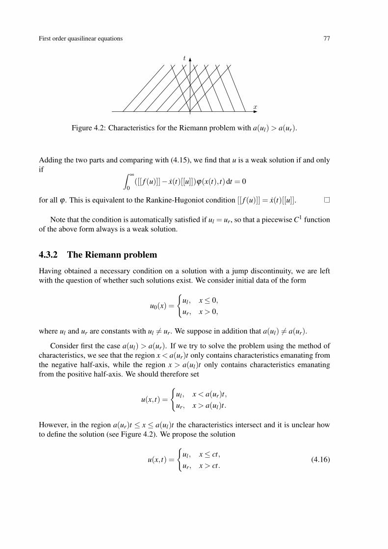
First order quasilinear equations 77
x
t
Figure 4.2: Characteristics for the Riemann problem with a(ul)> a(ur).
Adding the two parts and comparing with (4.15), we find that u is a weak solution if and onlyif ∫
∞
0([[ f (u)]]− x(t)[[u]])ϕ(x(t), t)dt = 0
for all ϕ . This is equivalent to the Rankine-Hugoniot condition [[ f (u)]] = x(t)[[u]].
Note that the condition is automatically satisfied if ul = ur, so that a piecewise C1 functionof the above form always is a weak solution.
4.3.2 The Riemann problem
Having obtained a necessary condition on a solution with a jump discontinuity, we are leftwith the question of whether such solutions exist. We consider initial data of the form
u0(x) =
ul, x≤ 0,ur, x > 0,
where ul and ur are constants with ul 6= ur. We suppose in addition that a(ul) 6= a(ur).
Consider first the case a(ul) > a(ur). If we try to solve the problem using the method ofcharacteristics, we see that the region x < a(ur)t only contains characteristics emanating fromthe negative half-axis, while the region x > a(ul)t only contains characteristics emanatingfrom the positive half-axis. We should therefore set
u(x, t) =
ul, x < a(ur)t,ur, x > a(ul)t.
However, in the region a(ur)t ≤ x ≤ a(ul)t the characteristics intersect and it is unclear howto define the solution (see Figure 4.2). We propose the solution
u(x, t) =
ul, x≤ ct,ur, x > ct.
(4.16)

78 First order quasilinear equations
x
t
x
u
cul
ur
Figure 4.3: Shock wave and corresponding characteristics. Here a(ul)> a(ur).
x
t
Figure 4.4: Characteristics for the Riemann problem with a(ul)< a(ur).
Clearly u solves (4.11) on either side of the discontinuity. From the previous discussion, wesee that u is a weak solution if and only if the Rankine-Hugoniot condition
c =[[ f (u)]][[u]]
(4.17)
is satisfied. The solution defined in (4.16)–(4.17) is called a shock wave.
Consider next the case a(ul)< a(ur) and assume for simplicity that a is strictly monotone(see e.g. Holden and Risebro [10] for the general case). We no longer have the problem thatcharacteristics cross. Instead we have the problem that no characteristics emanating fromthe x-axis enter the region a(ul)t ≤ x ≤ a(ur)t. Thus, it is again unclear how to define thesolution in this region. The shock solution (4.16)–(4.17) is still a weak solution even if ul < ur.However, we can also define a solution by setting
u(x, t) =
ul, x≤ a(ul)t,a−1(x/t), a(ul)t ≤ x≤ a(ur)t,ur, x≥ a(ur)t.

First order quasilinear equations 79
x
t
x
t
ul
ur
a(ur)
a(ul)
Figure 4.5: A rarefaction wave and corresponding characteristics.
Indeed, it is straight-forward to show that this defines a piecewise C1 function, which satisfiesthe differential equation in each of the three different regions. It follows that it is a weaksolution. We thus have the unhappy situation that weak solutions are not unique. The functionu is called a rarefaction wave. Figure 4.5 shows a rarefaction wave corresponding to Burgers’equation, for which a−1(x/t) = x/t and solution is given by a straight line in the intervala(ul)t ≤ x≤ a(ur)t.
4.3.3 Entropy conditionsThere is now way to single out the ‘correct’ solution by simply using the PDE. Precisely aswhen we introduced weak solutions above, we have to go back to the physics behind themodel to find a criterion. A common way of singling out the physically relevant solutionis to introduce some form of entropy condition. The name comes from the equations of gasdynamics, where these conditions have a physical interpretation. The basic idea is to introducea direction of time. Note that the original conservation law (4.11) is reversible, in the sensethat if u(x, t) is a solution, then so is u(−t,−x). Thus the qualitative behavior forward andbackward in time should be identical. This is in contrast to the heat equation ut = uxx. Aswe saw in Chapter 3, the heat equation is well-posed forward in time, but not backward intime. Thus, there is a ‘preferred’ sense of direction. This is also illustrated by the fact that forthe heat equation the L2-norm is strictly decreasing for solutions in S (R) (see Section 3.1.4),whereas it is conserved for Schwartz class solutions of the conservation law (4.11). Arguingthat there always is some diffusion or dissipation in a real physical system, one imposes thecondition that the ‘correct’ solution should be a limit as ε→ 0+ of a solution uε of the equation
ut + f (u)x = εuxx, ε > 0. (4.18)
Since this is difficult to verify directly, we now derive a necessary condition on u for thisto hold, wich is easier to check. Suppose that η is a C1 function and define q by q′(u) =

80 First order quasilinear equations
f ′(u)η ′(u). It is then easily confirmed that if u is a classical solution of the conservation law,then η(u)t + q(u)x = 0. Suppose now that η is C2 and convex so that η ′′(u) ≥ 0. We willshow that η(u)t +q(u)x ≤ 0 in a suitable weak sense if u is a weak solution obtained as a limitof C2 solutions of (4.18). We assume that uε → u in L1
loc(R2+) and that uε is locally bounded
uniformly in ε . Note that we don’t prove that such a convergence result holds; the main pointis to motivate condition (4.19) below. Multiplying (4.18) by η ′(uε)ϕ , where ϕ ∈C∞
0 (R2+) with
ϕ ≥ 0, we find that
0 =∫∫
R2+
(uεt + f (uε)x− εuε
xx)η′(uε)ϕ dxdt
=∫∫
R2+
(η(uε)t +q(uε)x− εη′(uε)uε
xx)ϕ dxdt
=∫∫
R2+
(−η(uε)ϕt−q(uε)ϕx)dxdt + ε
∫∫R2+
(η ′′(uε)(uεx)
2ϕ−η(uε)ϕxx)dxdt,
so that ∫∫R2+
(−η(uε)ϕt−q(uε)ϕx)dxdt ≤ ε
∫∫R2+
η(uε)ϕxx dxdt.
In the limit as ε → 0+ we therefore find that∫∫R2+
(−η(u)ϕt−q(u)ϕx)dxdt ≤ 0 (4.19)
for every ϕ ∈C∞0 (R2
+) with ϕ ≥ 0. This is sometimes expressed as saying that η(u)t +q(u)x≤0 in the sense of distributions. The pair (η ,q) is called an entropy-flux pair.
Definition 4.13. A weak solution u is said to be entropy admissible if (4.19) holds for everyentropy-flux pair (η ,q).
For a fixed number u?, the function ηδ (u) = ((u− u?)2 + δ 2)1/2 is convex and C∞. Itconverges to |u− u?| as δ → 0. Choosing the corresponding flux function qδ appropriately,we find that
qδ (u) =∫ u
u?
f ′(s)(s−u?)((s−u?)2 +δ 2)1/2 ds
→∫ u
u?f ′(s)sgn(s−u?)ds
= ( f (u)− f (u?))sgn(u−u?)
pointwise as δ → 0 by dominated convergence. Note that η(u) = |u− u?| is convex andsmooth everywhere except at u?, and that q(u) = ( f (u)− f (u?))sgn(u−u?) satisfies q′(u) =f ′(u)η ′(u) for u 6= u?. Thus (η ,q) can be thought of as a Lipschitz continuous entropy-flux

First order quasilinear equations 81
pair. Approximating (η ,q) with (ηδ ,qδ ) in (4.20) and passing to the limit using the dominatedconvergence theorem, one obtains the inequality∫∫
R2(|u−u?|ϕt + sgn(u−u?)( f (u)− f (u?))ϕx)dxdt ≥ 0
for every u? ∈ R. This is Kružkov’s admissibility condition. One can in fact show thatKružkov’s condition is equivalent to the entropy condition in Definition 4.13.
The entropy condition turns out to be exactly what is needed to prove existence and unique-ness. The proof of the following theorem is beyond the scope of these notes. See e.g. Bressan[4] and Hörmander [11].
Theorem 4.14. Assume that u0 ∈ L∞(R) and that f is locally Lipschitz continuous. Thereexists a unique entropy admissible weak solution u ∈ C([0,∞);L1
loc(R))∩ L∞(R× [0,∞)) ofthe Cauchy problem (4.11)–(4.12). If in addition u0 ∈ L1(R), then u ∈ C([0,∞);L1(R)) andthe map S(t) : u0 7→ u(·, t) from initial data to solution extends to a continuous semigroup onL1(R) with ‖S(t)u0−S(t)v0‖L1(R) ≤ ‖u0− v0‖L1(R).
We consider now the Riemann problem and show how the admissibility condition canbe used to single out a unique solution. The argument used to prove the Rankine-Hugoniotcondition shows that (4.19) leads to the jump condition
[[q(u)]]≤ c[[η(u)]] (4.20)
for every C1 entropy-flux pair (η ,q). Once again, the condition is automatically satisfied bya piecewise C1 solution. This means e.g. that a rarefaction wave is always admissible. Alimiting procedure shows again that the inequality continues to hold if we take η(u) = |u−u?|and q(u) = sgn(u−u?)( f (u)− f (u?)), whence we obtain
sgn(ur−u?)( f (ur)− f (u?))− sgn(ul−u?)( f (ul)− f (u?))≤ c(|ur−u?|− |ul−u?|).
Suppose that ul < ur and take u? = αul +(1−α)ur for α ∈ [0,1], so that u? ∈ [ul,ur]. We thenobtain the chain of inequalities
f (ur)+ f (ul)−2 f (u?)≤ c(ur +ul−2u?)⇒ f (ur)+ f (ul)−2 f (u?)≤ c(1−2α)(ur−ul)
⇒ f (ur)+ f (ul)−2 f (u?)≤ (1−2α)( f (ur)− f (ul))
⇒α f (ur)+(1−α) f (ul)≤ f (αul +(1−α)ur),
where we used the Rankine-Hugoniot condition in the third line. We leave it as an exercise toshow that the inequality is reversed if ur < ul . The conditions
α f (ur)+(1−α) f (ul)≤ f (αul +(1−α)ur), α ∈ [0,1],
if ul < ur, and
α f (ur)+(1−α) f (ul)≥ f (αul +(1−α)ur), α ∈ [0,1],

82 First order quasilinear equations
if ur < ul , are called the Lax shock conditions. They have a very simple geometric interpre-tation, saying that the graph of f must lie above the line segment between (ul, f (ul)) and(ur, f (ur)) in the first case and below the line segment in the second case. In particular, if f isconvex, we obtain the condition
ur < ul
for a shock. For the Riemann problem, this means that the shock is the correct entropy solutionin the case ur < ul , whereas the rarefaction wave is the correct entropy solution in the caseul < ur. The condition is reversed if f is concave.
Example 4.15. Consider the traffic model from Example 4.9, written in the normalized formut + f (u)x = 0, where f (u) = u(1−u) is concave. This means that a shock wave will form iful < ur (meaning that the density is greater in the direction of the traffic). Consider e.g. thecase when ur = 1 meaning that the cars are standing still ahead.This might e.g. model a queueforming at a red light. The velocity of the shock will then be c = ( f (ur)− f (ul))/(ur−ul)< 0(assuming that ul ∈ (0,1)), so the shock wave is moving backwards, that is cars driving towardsthe traffic light are coming to a sudden stop. If on the other hand ul > ur we get a rarefactionwave. If ul = 1, this might model what happens when the light turns green.
Chapter 5
Distributions and Sobolev spaces
In the previous chapter we encountered weak solutions of PDE. The key was to multiply theequation by a ‘test function’ ϕ ∈ C∞
0 (Rd) and integrate by parts to put all the derivatives onϕ . The name test function refers to the fact that the equation is ‘tested’ against ϕ . This givesa suitable definition of weak solutions in which the solution u doesn’t need to be differen-tiable. If u is a sufficiently regular weak solution, one shows that it is a classical solution,meaning that the PDE holds pointwise. What is involved here is the concept of ‘weak’ or‘distributional’ derivatives. The weak derivative of a non-differentiable function is in generalnot a function, but a distribution. The purpose of this chapter is partly to clarify what thismeans. Distributions or ‘generalized functions’ have a long prehistory. The theory was maderigorous in the middle of the 20th century, in particular by Laurent Schwartz (1915–2002).Distributions are indispensable in the modern theory of linear partial differential equations.
Distributions are not quite as useful for nonlinear equations, since one can in generalnot define the product of two distributions. Moreover, the space of distributions is not anormed vector space. For this purpose we introduce a generalization of Lebesgue spacescalled Sobolev spaces after Sergei L’vovich Sobolev (1908–1989). Sobolev was also involvedin the early theory of distributions. The Sobolev space Hk simply consists of L2 functionswhose weak derivatives up to order k lie in L2. As we will see, Hk is a Banach space andmoreover an algebra if k is sufficiently large. Another important reason for using Sobolevspaces is that they behave well with respect to the Fourier transform. This is not the case forspaces based on the supremum norm.
The present chapter can only serve as brief introduction. For more details on distribu-tions we refer to Friedlander [9], Duistermaat and Kolk [6], Hörmander [12], Rauch [20] andStrichartz [25]. For more on Sobolev spaces we refer to the standard reference Adams andFournier [1]. In particular, this reference discusses Sobolev spaces on subsets of Rd , wherethe regularity of the boundary plays an important role. In these notes we shall only discussSobolev spaces on Rd .
83

84 Distributions and Sobolev spaces
5.1 DistributionsNote that a locally integrable function u∈L1
loc(Rd) gives rise to a linear functional1 `u : C∞0 (Rd)→
C defined by `u(ϕ) = 〈u,ϕ〉, where
〈u,ϕ〉 :=∫Rd
u(x)ϕ(x)dx. (5.1)
Note that this differs from the inner product in L2(Rd) in that there is no complex conjugateon ϕ and that we don’t require u,ϕ ∈ L2(Rd). It is clear at least if u is continuous that `udetermines u uniquely, since if `u(ϕ) = 0 for all ϕ ∈ C∞
0 (Rd) then u ≡ 0. Below we shallprove that this is also the case if u ∈ L1
loc(Rd).
In keeping with the notation of Laurent Schwartz, we denote the space of test functionsC∞
0 (Rd) by D(Rd).
Definition 5.1. A distribution ` is a linear functional on D(Rd) which is continuous in thefollowing sense. If ϕn ⊂D(Rd) has the following properties:
(1) there exists a compact set K ⊂ Rd such that suppϕn ⊆ K for all n, and
(2) there exists a function ϕ ∈D(Rd) such that for all α ∈ Nd , ∂ αϕn→ ∂ αϕ uniformly,
then `(ϕn)→ `(ϕ) as n→ ∞. The space of distributions is denoted D ′(Rd).
Remark 5.2. D ′(Rd) is simply the space of continuous linear functionals on D(Rd) whenD(Rd) is given the topology defined by (1) and (2) in the above definition. When (1) and (2)hold, we say that ϕn→ ϕ in D(Rd). One can define D(Ω) if Ω is an open subset of Rd in asimilar fashion.
The most common ways that distributions appear is through the expression (5.1). The factthat this expression defines a distribution follows from the estimate
|〈u,ϕ〉| ≤(∫
K|u(x)|dx
)‖ϕ‖L∞(Rd),
if ϕ ∈D(Rd) with suppϕ ⊆K. Let us prove that (5.1) determines the distribution `u uniquely.Note that by linearity, it suffices to show that that u = 0 (as an element of L1
loc(Rd)) if `u = 0.
Theorem 5.3. Let u ∈ L1loc(Rd). If 〈u,ϕ〉= 0 for all ϕ ∈D(Rd), then u(x) = 0 a.e.
Proof. It suffices to prove that u = 0 a.e. in the ball BR(0) ⊂ Rd for any R > 0. Let v =χB2R(0)u ∈ L1(Rd). Then
∫Rd v(x)ϕ(x)dx =
∫Rd u(x)ϕ(x)dx = 0 for any ϕ ∈ D(Rd) with
suppϕ ⊂ B2R(0). Let J be a mollifier as in Theorem B.25. Then Jε ∗ v→ v in L1(Rd) by The-orem B.25 (4) and hence also in L1(BR(0)). On the other hand, (Jε ∗ v)(x) =
∫Rd v(y)Jε(x−
y)dy = 0 for x ∈ BR(0) and ε > 0 sufficiently small, since suppJε(x−·)⊂ BR+ε(0). It followsthat u = v = 0 a.e. in BR(0).
1A linear functional is just a linear map with values in C.

Distributions and Sobolev spaces 85
The above theorem implies that we can identify u with the linear functional `u. We will dothis without further mention in what follows. We shall also use the notation 〈u,ϕ〉 for u(ϕ)even when u is just an element of D ′(Rd). Let us give an example of a distribution which doesnot correspond to a locally integrable function.
Example 5.4. The Dirac2 distribution δa at a ∈ Rd is defined by
〈δa,ϕ〉 := ϕ(a).
It is clear that 〈δa,ϕn〉 = ϕn(a)→ ϕ(a) = 〈δa,ϕ〉 if ϕn→ ϕ in D(Rd), so that δa really is adistribution. It is also clear that δa doesn’t correspond to a locally integrable function, since〈δa,ϕ〉 = 0 if ϕ(a) = 0. If 〈δa,ϕ〉 = 〈u,ϕ〉 for some u ∈ L1
loc(Rd), this would imply thatu(x) = 0 a.e. and hence that 〈δa,ϕ〉= 〈u,ϕ〉= 0 for all ϕ ∈D(Rd).
We also need to know what is meant by convergence of a sequence of distributions.
Definition 5.5. We say that un→ u in D ′(Rd) if 〈un,ϕ〉 → 〈u,ϕ〉 for all ϕ ∈D(Rd)
Example 5.6. Consider a function K ∈L1(Rd) with∫Rd K(x)dx= 1 and set Kε(x)= ε−dK(ε−1x)
for ε > 0. Then Kε→ δ0 as ε→ 0 since 〈Kε ,ϕ〉=∫Rd Kε(y)ϕ(y)dy= (Kε ∗R(ϕ))(0)→ ϕ(0)
as ε → 0+ by Theorem B.27, where R(ϕ)(x) = ϕ(−x). In particular, we have that Kt → δ0as t→ 0+, where Kt is the heat kernel.
5.2 Operations on distributionsWe now discuss how to extend various operations on functions to distributions. To explain themethod, we consider translations in x. Given a function ϕ ∈ D(Rd) and a vector h ∈ Rd , wedefine (τhϕ)(x) = ϕ(x−h). If ϕ,ψ ∈D(Rd) we have that
〈τhϕ,ψ〉=∫Rd
ϕ(x−h)ψ(x)dy =∫Rd
ϕ(y)ψ(y+h)dx = 〈ϕ,τ−hψ〉.
It therefore makes sense to define
〈τhu,ϕ〉 := 〈u,τ−hϕ〉 (5.2)
if u is just a distribution. Note that τ−hϕn→ τ−hϕ if ϕn→ ϕ in D(Rd), so that (5.2) indeeddefines a distribution τhu. It is clear that the new definition agrees with the old one if u ∈D(Rd) in the sense that the distribution τhu defined by (5.2) can be represented by the functionu(·−h).
Example 5.7. We have τhδ0 = δh, since
〈τhδ0,ϕ〉= 〈δ0,τ−hϕ〉= ϕ(0+h) = ϕ(h).
2After the physicist Paul Dirac (1902–1984).

86 Distributions and Sobolev spaces
The above extension of the translation operator is an example of a general principle.
Proposition 5.8. Suppose that L is a linear operator on D(Rd) which is continuous in thesense that ϕn → ϕ in D(Rd) implies L(ϕn)→ L(ϕ). Suppose, moreover, that there exists acontinuous linear operator LT on D(Rd), with the property that 〈L(ϕ),ψ〉 = 〈ϕ,LT (ψ)〉 forall ϕ,ψ ∈D(Rd). Then L extends to a continuous linear operator on D ′(Rd) given by
〈L(u),ϕ〉= 〈u,LT (ϕ)〉 for all u ∈D ′(Rd) and ϕ ∈D(Rd). (5.3)
Proof. The continuity of LT shows that L(u) defined in (5.3) is a distribution. It is also clearfrom the definition of the transpose that (5.3) defines an extension of the original operator L.Finally, if un→ u in D ′(Rd), then
〈L(un),ϕ〉= 〈un,LT (ϕ)〉 → 〈u,LT (ϕ)〉= 〈L(u),ϕ〉,
so the extension is continuous on D ′(Rd).
We call the operator LT the transpose of L. Note that this might differ from the L2 adjointsince there is no complex conjugate on ψ in 〈ϕ,ψ〉. We now give a list of common operatorsand their transposes. Here (σλ ϕ)(x) = ϕ(λx) is dilation by λ ∈ R \ 0 and (Mψϕ)(x) =ψ(x)ϕ(x) multiplication by ψ ∈C∞(Rd).
L LT
τh τ−hσλ |λ |−dσ1/λ
Mψ Mψ
∂ α (−1)|α|∂ α
As a corollary to Proposition 5.8 we therefore have the following result.
Proposition 5.9. Each of the operators τh, σλ , Mψ and ∂ α on D(Rd) have unique extensionsto continuous maps on D ′(Rd). The extensions are given by 〈Lu,ϕ〉= 〈u,LT ϕ〉 where L andLT are as in the above table.
Note the restriction to multiplication with smooth functions. In general we can’t define theproduct of a distribution and a non-smooth function ψ since then ϕψ 6∈D(Rd). In particular,one can in general not define the product of two distributions. We will get back to this questionlater on.
Example 5.10. The Heaviside3 function
H(x) =
1 x > 0,0 x≤ 0,
3After the physicist Oliver Heaviside (1850–1925).

Distributions and Sobolev spaces 87
is locally integrable and hence H ∈D ′(R). The distributional derivative of H is calculated asfollows:
〈H ′,ϕ〉=−〈H,ϕ ′〉=−∫
∞
0ϕ′(x)dx = ϕ(0) = 〈δ0,ϕ〉.
It follows that H ′ = δ0 ∈ D ′(R). Note that the pointwise derivative of H is zero everywhereexcept at 0, where it is undefined. We can continue the process and calculate higher derivativesof H. E.g.
〈H ′′,ϕ〉= 〈δ ′0,ϕ〉=−〈δ0,ϕ′〉=−ϕ
′(0).
5.3 Tempered distributionsOne operation which can not be defined on D ′(Rd) is the Fourier transform. As the followinglemma shows, F is its own transpose.
Lemma 5.11. For ϕ,ψ ∈S (Rd), we have that
〈F (ϕ),ψ〉= 〈ϕ,F (ψ)〉.
Proof. The result can be proved using Lemma 2.15, but it is simpler to give a direct proof. ByFubini’s theorem we have that
〈F (ϕ),ψ〉= (2π)−d/2∫Rd
(∫Rd
ϕ(x)e−ix·ξ dx)
ψ(ξ )dξ
= (2π)−d/2∫Rd
ϕ(x)(∫
Rdψ(ξ )e−ix·ξ dξ
)dx
= 〈ϕ,F (ψ)〉.
The problem with defining 〈F (u),ϕ〉= 〈u,F (ϕ)〉 is that F doesn’t map D(Rd) to itself(compact support is lost). The key is to instead use S (Rd) as the space of test functions.
Definition 5.12. A continuous linear functional on S (Rd) is called a tempered distribution4.The space of tempered distributions is denoted S ′(Rd).
Convergence in S ′(Rd) is defined analogously to convergence in D ′(Rd).
Definition 5.13. We say that un→ u in S ′(Rd) if un(ϕ)→ u(ϕ) for all ϕ ∈S (Rd)
Continuity of an element u ∈S ′(Rd) means that
〈u,ϕn〉 → 〈u,ϕ〉
if ϕn→ ϕ in S (Rd). If u ∈S ′(Rd), then 〈u,ϕ〉 is well-defined if ϕ ∈ D(Rd). Moreover, ifϕn→ ϕ ∈D(Rd), then clearly ϕn→ ϕ in the topology of S (Rd). Consequently, the restric-tion of a tempered distribution to D(Rd) is an element of D ′(Rd). Moreover, u is uniquely
4Sometimes called a temperate distribution.

88 Distributions and Sobolev spaces
determined by its restriction to D(Rd), since D(Rd) is a dense subspace of S (Rd) (Proposi-tion 2.2 (5)). It therefore makes sense to write S ′(Rd) ⊂ D ′(Rd). The inclusion is strict, inthe sense that there exist elements u ∈D ′(Rd) which can not be extended to continuous linearfunctionals on S (Rd).
Example 5.14.
(1) The Dirac distribution δa belongs to S ′(Rd).
(2) Any locally integrable function u with (1+ | · |2)−Nu ∈ L1(Rd) for some N belongs toS ′(Rd) since∫
Rd|u(x)ϕ(x)|dx≤
∫Rd(1+ |x|2)−N |u(x)|(1+ |x|2)N |ϕ(x)|dx
≤ ‖(1+ | · |2)−Nu‖L1(Rd)‖(1+ | · |2)N
ϕ‖L∞(Rd).
(3) In particular, any u ∈ Lp(Rd), p ∈ [1,∞], belongs to S ′(Rd) since (1+ | · |2)−Nu ∈L1(Rd) if N is sufficiently large by Hölder’s inequality.
(4) u(x) = e|x| is in D ′(Rd) but not in S ′(Rd). Strictly speaking this means that the func-tional ϕ 7→ 〈u,ϕ〉, ϕ ∈D(Rd), can not be extended to an element of S ′(Rd). This cane.g. be seen by approximating a function ϕ ∈S (Rd) satisfying ϕ(x) = e−|x|/2 for large|x| with a sequence in D(Rd) in the topology of S (Rd).
The proof of the following result is exactly the same as the proof of Proposition 5.8.
Proposition 5.15. The result in Proposition 5.8 remains true if D(Rd) is replaced by S (Rd)and D ′(Rd) by S ′(Rd).
As a consequence, Proposition 5.9 holds also for S ′(Rd) if we in the definition of themultiplication operator assume that ψ ∈S (Rd), so that ψϕ ∈S (Rd) if ϕ ∈S (Rd). Moregenerally, one can assume that ψ and its derivatives grow at most polynomially.
Proposition 5.16. Let ψ ∈C∞(Rd) and assume that ψ and its derivative grow at most poly-nomially. Each of the operators τh, σλ , Mψ and ∂ α on S (Rd) extend to continuous operatorson S ′(Rd).
Alternatively, one can view these operators as restrictions of the corresponding operators onD ′(Rd) to S ′(Rd).
The main purpose of introducing tempered distributions is to extend the Fourier trans-form. The fact that F : S (Rd)→S (Rd) is continuous shows that following definition makessense.

Distributions and Sobolev spaces 89
Definition 5.17. The Fourier transform on S ′(Rd) is the continuous operator F : S ′(Rd)→S ′(Rd) defined by
〈F (u),ϕ〉 := 〈u,F (ϕ)〉,
for u ∈ S ′(Rd) and ϕ ∈ S (Rd). The inverse Fourier transform is the continuous operatorF−1 : S ′(Rd)→S ′(Rd) defined by
〈F−1(u),ϕ〉 := 〈u,F−1(ϕ)〉.
It follows easily from the definition of F−1 on S (Rd) that F−1 = RF = FR. Asusual, we write u for F (u) also if u ∈S ′(Rd). The following properties are analogous to theones in Proposition 2.6.
Proposition 5.18. For u ∈S ′(Rd), we have that
τ−yu F7→ eiy·ξ u,
eiy·xu F7→ τyu,
σλ u F7→ |λ |−dσ1/λ u,
∂αx u F7→ (iξ )α u,
xα u F7→ (i∂ξ )α u,
where y ∈ Rd and λ ∈ R\0.
Proof. The identities follow by combining the definitions of these operators in terms of theirtransposes with the corresponding properties for Schwartz class functions. We illustrate themethod by proving the first identity and leave the others to the reader. Considering ϕ as afunction of ξ we have that
〈F (τ−yu),ϕ〉= 〈τ−yu, ϕ〉= 〈u,τyϕ〉= 〈u,F (eiy·ξϕ)〉= 〈u,eiy·ξ
ϕ〉= 〈eiy·ξ u,ϕ〉.
Theorem 5.19. F : S ′(Rd)→S ′(Rd) is an isomorphism with inverse F−1.
Proof. We simply note that
〈F−1F (u),ϕ〉= 〈F (u),F−1(ϕ)〉= 〈u,FF−1(ϕ)〉= 〈u,ϕ〉.
Similarly, 〈FF−1(u),ϕ〉= 〈u,F−1F (ϕ)〉= 〈u,ϕ〉.
Example 5.20. We have 〈δ0,ϕ〉= 〈δ0, ϕ〉= ϕ(0) = (2π)−d/2 ∫Rd ϕ(x)dx, so δ0 = (2π)−d/2.
By Fourier’s inversion formula it follows that F (1)=RF−1(1)= (2π)d/2R(δ0)= (2π)d/2δ0.

90 Distributions and Sobolev spaces
In order to extend convolutions to S ′(Rd) we first prove that ϕ ∗ is a continuous linearoperator on S (Rd) for a fixed ϕ ∈S (Rd).
Lemma 5.21. Assume that ϕ ∈S (Rd) and that ψn→ ψ in S (Rd). Then ϕ ∗ψn→ ϕ ∗ψ inS (Rd).
Proof. From the convolution theorem it follows that F (ϕ ∗ψn) = (2π)d/2ϕψn. The resultfollows since Mϕ , F and F−1 are continuous operators on S (Rd).
The transpose of ϕ ∗ is computed by changing the order of integration in 〈ϕ ∗u,ψ〉:∫Rd
(∫Rd
ϕ(x− y)u(y)dy)
ψ(x)dx =∫Rd
u(y)(∫
Rdϕ(x− y)ψ(x)dx
)dy
if u ∈S (Rd), so that (ϕ ∗)T = R(ϕ)∗, where as usual R(ϕ)(x) = ϕ(−x).
Proposition 5.22. For ϕ ∈ S (Rd), the operator ϕ ∗ extends to a continuous operator onS ′(Rd) given by 〈ϕ ∗u,ψ〉 := 〈u,R(ϕ)∗ψ〉. The extension satisfies
F (ϕ ∗u) = (2π)d/2ϕ u,
∂α(ϕ ∗u) = (∂ α
ϕ)∗u = ϕ ∗ (∂ αu).
Proof. The existence of the extension is a consequence of Proposition 5.15 and Lemma 5.21.The identity F (ϕ ∗u) = (2π)d/2ϕ u follows from the calculation
〈F (ϕ ∗u),ψ〉= 〈ϕ ∗u, ψ〉= 〈u,R(ϕ)∗ ψ〉= 〈u,FF−1(R(ϕ)∗ ψ)〉= 〈u,F−1(R(ϕ)∗ ψ)〉= 〈u,(2π)d/2
ϕψ〉= 〈(2π)d/2
ϕ u,ψ〉,
in which the convolution theorem for S (Rd) and the relation F−1 = FR = RF have beenused. The second identity follows from similar manipulations and its proof is left to thereader.
Since convolution is commutative on S (Rd) we shall also write u ∗ϕ instead of ϕ ∗ u.Keeping u fixed and varying ϕ we obtain a continuous linear operator from S (Rd) to S ′(Rd).Note that u∗ v is in general not well-defined if u,v ∈S ′(Rd).
Example 5.23. We have 〈δ0 ∗ϕ,ψ〉= 〈δ0,R(ϕ)∗ψ〉=∫Rd ϕ(x)ψ(x)dx = 〈ϕ,ψ〉. Thus, δ0 ∗
is the identity on S (Rd). Similarly, (∂ αδ0)∗= ∂ α on S (Rd).
Example 5.24. If Kε is as in Example 5.6, we find that Kε ∗ϕ → δ0 ∗ϕ = ϕ in S ′(Rd). Thisagrees with what we already know about Kε .

Distributions and Sobolev spaces 91
5.4 Approximation with smooth functionsThere is an important question that we have avoided. In Propositions 5.9 and 5.15 we didn’tsay anything about the uniqueness of the extensions. The extensions are in fact unique, but toprove this one has to show that D(Rd) is dense in D ′(Rd) in the first case and that S (Rd)is dense S ′(Rd) in the second case. This is done by the usual procedure of mollification andmultiplication with smooth ‘cut-off’ functions, but there are some technical details. We willpresent the proofs for the interested reader. The section may be skipped on a first reading sincethe results are not used elsewhere in the notes.
We begin by noting that the definition 〈u∗ϕ,ψ〉 := 〈u,R(ϕ)∗ψ〉 also makes sense whenu ∈ D ′(Rd) and ϕ,ψ ∈ D(Rd), since then R(ϕ) ∗ψ ∈ D(Rd) (see Section B.5). There ishowever another natural way of defining convolutions. We show that these two definitionsagree.
Lemma 5.25. For u ∈D ′(Rd) and ϕ ∈D(Rd) we have that u∗ϕ ∈C∞(Rd) with
(u∗ϕ)(x) = 〈u,τxR(ϕ)〉= 〈u,ϕ(x−·)〉.
Proof. Since x 7→ ϕ(x−·) is continuous from Rd to D(Rd) it follows that x 7→ 〈u,ϕ(x−·)〉 ∈C(Rd). Moreover, limh→0 h−1(ϕ(x + he j − ·)− ϕ(x− ·)) = ∂ jϕ(x− ·) in D(Rd) for eachx and j, and x 7→ ∂ jϕ(x− ·) is continuous from Rd to D(Rd). From this it follows thatx 7→ 〈u,ϕ(x− ·)〉 ∈ C1(Rd). Proceeding by induction, one shows that x 7→ 〈u,ϕ(x− ·)〉 ∈C∞(Rd). The result therefore follows if we prove the equality (u ∗ϕ)(x) = 〈u,ϕ(x−·)〉. Letv(x) = 〈u,ϕ(x−·)〉. Using Riemann sums we find that
〈v,ψ〉=∫Rd
v(x)ψ(x)dx
= limn→∞
∑α∈Zd
ψ(α/n)〈u,ϕ(α/n−·)〉n−d
=
⟨u, lim
n→∞∑
α∈Zd
ψ(α/n)ϕ(α/n−·)n−d
⟩= 〈u,R(ϕ)∗ψ〉
for ψ ∈D(Rd), where we have used the fact that ∑α∈Zd ψ(α/n)ϕ(α/n−·)n−d→R(ϕ)∗ψ inD(Rd) (left as an exercise for the reader). The expression on the last line is simply 〈u∗ϕ,ψ〉,so this proves the equality u∗ϕ = v.
Theorem 5.26. D(Rd) is dense in S ′(Rd) and D ′(Rd).
Proof. We first approximate u ∈ D ′(Rd) with the sequence ψ(·/n)u in D ′(Rd), where ψ ∈D(Rd) with ψ(x) = 1 for |x| ≤ 1. It is clear that ψ(·/n)ϕ → ϕ in D(Rd) if ϕ ∈ D(Rd)(they are equal for large n) and hence ψ(·/n)u→ u in D ′(Rd). Similarly, if u ∈S ′(Rd), thesequence converges to u in S ′(Rd). We can therefore replace u by ψu, for some functionψ ∈ D(Rd), in what follows. We define un = (ψu) ∗ J1/n, where J is an even mollifier (see

92 Distributions and Sobolev spaces
Section B.5). By the previous lemma it follows that un ∈ C∞(Rd) as an element of D ′(Rd).Moreover, un has compact support since un(x) = 〈ψu,J1/n(x− ·)〉 = 〈u,ψJ1/n(x− ·)〉 = 0 ifdist(x,suppψ)≥ 1/n. Finally,
〈un,ϕ〉= 〈ψu,J1/n ∗ϕ〉= 〈ψu, ψ(J1/n ∗ϕ)〉,
where ψ ∈ D(Rd) with ψ = 1 on suppψ . We have that ∂ α(J1/n ∗ϕ) = J1/n ∗ ∂ αϕ → ∂ αϕ
uniformly. Hence ψ(J1/n ∗ϕ)→ ψϕ in D(Rd) and un→ ψu in D ′(Rd). To prove the sameconvergence in the topology of S ′(Rd), we first note that 〈(ψu)∗ J1/n,ϕ〉 is given by 〈w,ϕ〉,where w(x) = 〈u,J1/n(x−·)〉 is in D(Rd), whenever ϕ ∈ D(Rd). However, since D(Rd) isdense in S (Rd) and w has compact support, the same is true by an approximation argumentwhenever ϕ ∈S (Rd). We still have that ∂ α(J1/n ∗ϕ) = J1/n ∗ ∂ αϕ → ∂ αϕ uniformly andhence ψ(J1/n ∗ϕ)→ ψϕ in S (Rd). It follows that un→ ψu in S ′(Rd).
Corollary 5.27. The extensions in Propositions 5.9 and 5.15 are unique.
Example 5.28. Consider the three-dimensional wave equation. For initial data u0 = 0 andu1 ∈S (Rd) the solution is expressed on the Fourier side as sin(t|ξ |)
|ξ | u1(ξ ). Note that sin(t|·|)|·| ∈
S ′(Rd). By Proposition 5.22 we therefore have that
u(x, t) = (2π)−3/2F−1(
sin(t|ξ |)|ξ |
)∗u1
in the sense of distributions. At least if u1 ∈D(Rd), we can make sense of (2π)−3/2F−1(
sin(t|ξ |)|ξ |
)∗
u1 as〈vt ,u1(x−·)〉,
where vt = (2π)−3/2F−1(
sin(t|ξ |)|ξ |
)∈ S ′(Rd). The distribution vt is nothing but tMt from
Section 3.2, that is,
〈vt ,ϕ〉= tMt(ϕ) =1
4πt
∫|x|=|t|
ϕ(x)dS(x).
5.5 Sobolev spacesDefinition 5.29. The Sobolev space Hk(Rd) is the space of u∈ L2(Rd) such that ∂ αu∈ L2(Rd)for any |α| ≤ k, where the derivatives are interpreted in the sense of distributions.
The notation W k,2(Rd) is also frequently used instead of Hk(Rd). One then regardsHk(Rd) as a member of a more general family W k,p(Rd) of Sobolev spaces, in which L2(Rd)is replaced by Lp(Rd).
Note that(u,v)Hk(Rd) := ∑
|α|≤k
∫Rd
∂αu(x)∂ αv(x)dx

Distributions and Sobolev spaces 93
defines an inner product on Hk(Rd). Using the completeness of L2(Rd) and the definitionof distributional derivatives, it is easy to prove that Hk(Rd) is in fact a Hilbert space withthis inner product. Alternatively, one can prove this by first characterizing Hk(Rd) using theFourier transform. The following result is a direct consequence of Parseval’s formula.
Lemma 5.30. Let Pk(ξ ) = ∑|α|≤k ξ 2α . Then u ∈ L2(Rd) is in Hk(Rd) if and only if∫Rd
Pk(ξ )|u(ξ )|2 dξ < ∞. (5.4)
Moreover,
‖u‖2Hk(Rd) =
∫Rd
Pk(ξ )|u(ξ )|2 dξ . (5.5)
Proof. If u ∈ L2(Rd), then its distributional derivatives satisfy F (∂ αu) = (iξ )α u by Proposi-tion 5.18. If u ∈ Hk(Rd), we therefore obtain the equality (5.5) which implies (5.4). On theother hand, if (5.4) holds, we obtain that all the derivatives of order less than or equal to k arein L2(Rd). We therefore obtain that u ∈ Hk(Rd) and that (5.5) holds.
This result suggests a generalization of the Sobolev spaces. We introduce the notation〈ξ 〉= (1+ |ξ |2)1/2. Note that Pk(ξ )∼ 〈ξ 〉2k in the sense that there exist constants C1,C2 > 0such that C1〈ξ 〉2k ≤ Pk(ξ )≤C2〈ξ 〉2k for all ξ ∈ Rd . We can therefore replace Pk(ξ ) by 〈ξ 〉2k
in the definition of the norm of Hk(Rd). This allows us to extend the definition of Sobolevspaces to non-integer indices and to negative indices.
Definition 5.31. Let s ∈ R. Hs(Rd) is the space of tempered distributions u such that u ∈L1
loc(Rd) with
‖u‖Hs(Rd) :=(∫
Rd(1+ |ξ |2)s|u(ξ )|2 dξ
)1/2
< ∞. (5.6)
These spaces are usually called fractional Sobolev spaces (even though s doesn’t have tobe rational). From now on we will use (5.6) as the norm on Hs(Rd), even when s is a non-negative integer. Note that S (Rd)⊂Ht(Rd)⊂Hs(Rd)⊂S ′(Rd) when s < t, each inclusionbeing continuous.
Theorem 5.32. Hs(Rd) is a Hilbert space with inner product
(u,v)Hs(Rd) :=∫Rd(1+ |ξ |2)su(ξ )v(ξ )dξ .
Proof. It is clear that (·, ·)Hs(Rd) defines an inner product on Hs(Rd) with (u,u)Hs(Rd) =
‖u‖2Hs(Rd)
, so we only need to prove the completeness. This follows since the map T : u 7→〈ξ 〉su is an isometric isomorphism from Hs(Rd) to L2(Rd).
Note that the elements of Hs(Rd) need not be functions when s < 0.
94 Distributions and Sobolev spaces
Example 5.33. The distribution δ0 ∈ S ′(Rd) satisfies δ0 = (2π)−d/2. Using polar coordi-nates, we find that ∫
Rd(1+ |ξ |2)s dξ < ∞
if and only if s <−d/2. Hence δ0 ∈ Hs(Rd) if and only if s <−d/2.
Riesz’ representation theorem (Theorem A.12) implies that the dual space of Hs(Rd) canbe identified with Hs(Rd) itself. The element v ∈ Hs(Rd) is here identified with the boundedlinear functional
Hs(Rd) 3 u 7→ (u,v)Hs(Rd) =∫Rd(1+ |ξ |2)su(ξ )v(ξ )dξ . (5.7)
The dual can also be identified with H−s(Rd) using an extension of the usual pairing betweenS ′(Rd) and S (Rd). Rewriting
〈w,ϕ〉=∫Rd
w(ξ )ϕ(−ξ )dξ =∫Rd〈ξ 〉−sw(ξ )〈ξ 〉sϕ(−ξ )dξ ,
we see that 〈·, ·〉 extends to a bilinear map H−s(Rd)×Hs(Rd)→ C. It is also clear that thefunctional defined by v ∈ Hs(Rd) according to (5.7) is identical to the functional u 7→ 〈w,u〉where w := Λ2sC v, in which C v = v for v ∈S (Rd) and is extended by duality to S ′(Rd),and Λ2s := F−1M〈ξ 〉2sF : Hs(Rd)→ H−s(Rd). Whenever one identifies the dual with eitherHs(Rd) or H−s(Rd) one has to keep in mind how the identification is done.
Proposition 5.34. C∞0 (Rd) is dense in Hs(Rd).
Proof. We can approximate 〈ξ 〉su arbitrarily well by ϕ ∈ C∞0 (Rd) in L2(Rd). Hence, u is
approximated well by F−1(〈ξ 〉−sϕ) ∈S (Rd) in Hs(Rd). Since C∞0 (Rd) is dense in S (Rd)
it follows that C∞0 (Rd) is also dense in Hs(Rd).
In particular this implies that Hs(Rd) is the completion of C∞0 (Rd) with respect to the norm
‖ · ‖Hs(Rd). This gives an alternative way of introducing Sobolev spaces.
Sobolev spaces are typically used in connection with PDE. One usually proves the ex-istence of a solution in some Sobolev space. It is of interest to know when the solution issufficiently differentiable in the usual sense to define a classical solution of the PDE.
Definition 5.35. Ck(Rd) is the space of k times continuously differentiable functions u : Rd→C, such that lim|x|→∞ |∂ αu(x)| = 0 for all α ∈ Nd with |α| ≤ k, endowed with the norm‖u‖Ck
b(Rd) := max|α|≤k supRd |∂ αu(x)|.
Lemma 5.36. Ck(Rd) is a closed subspace of the Banach space Ckb(R
d).
Proof. Let un ⊂ Ck(Rd) with un→ u in Ckb(R
d). For ε > 0 we can find a number N suchthat ‖un−u‖Ck
b(Rd) < ε if n≥ N. Choosing R such that |∂ αuN(x)|< ε for |x| ≥ R and |α| ≤ k,
we find that |∂ αu(x)| ≤ |∂ αuN(x)|+‖u−uN‖Ckb(Rd) < 2ε if |x| ≥ R. Hence, u ∈ Ck(Rd).

Distributions and Sobolev spaces 95
Note that this means that Ck(Rd) is itself a Banach space.
Theorem 5.37 (Sobolev embedding theorem). Let k ≥ 0. Hs(Rd) is continuously embeddedin Ck(Rd) when s > k+ d
2 , meaning that Hs(Rd) ⊂ Ck(Rd) and that the inclusion map fromHs(Rd) to Ck(Rd) is continuous.
Proof. We begin by proving the inequality
‖ϕ‖Ckb(Rd) ≤C‖ϕ‖Hs(Rd)
for ϕ ∈ S (Rd) where C = C(k,s,d). For α ∈ Nd with |α| ≤ k it follows from Hölder’sinequality that
|∂ αϕ(x)| ≤ (2π)−d/2
∫Rd|ξ |k|ϕ(ξ )|dξ
= (2π)−d/2∫Rd
|ξ |k
(1+ |ξ |2)s/2
((1+ |ξ |2
)s/2 |ϕ(ξ )|)
dξ
≤ (2π)−d/2(∫
Rd
|ξ |2k
(1+ |ξ |2)s dξ
)1/2(∫Rd
(1+ |ξ |2
)s |ϕ(ξ )|2 dξ
)1/2
=C‖ϕ‖Hs(Rd),
where C = (2π)−d/2‖|ξ |k〈ξ 〉−s‖L2(Rd) < ∞ since |ξ |2k〈ξ 〉−2s ≤ 2|ξ |2(k−s) for large |ξ | and2(k− s)<−d. Taking the maximum over all α we find that
‖ϕ‖Ckb(Rd) ≤C‖ϕ‖Hs(Rd). (5.8)
Pick ϕn ⊂ S (Rd) with ϕn → f in Hs(Rd) as n→ ∞. The inequality ‖ϕn−ϕm‖Ckb(Rd) ≤
C‖ϕn−ϕm‖Hs(Rd) follows from (5.8) and implies that ϕn is a Cauchy sequence in Ck(Rd).Since Ck(Rd) is a Banach space it follows that ϕn converges to some element g in Ck(Rd).But then ϕn converges both to f and g in S ′(Rd) so f = g as distributions. It follows fromTheorem 5.3 that f = g a.e. Taking limits, one obtains (5.8) with f substituted for ϕ .
Remark 5.38. The elements of Hs(Rd) are actually equivalence classes, not functions. TheSobolev embedding theorem implies that, for s > k+ d/2, there is a continuous member ofeach such class. As usual we identify the equivalence class with the continuous representative.
Finally, we prove that Hs(Rd) is an algebra if s > d/2.
Theorem 5.39. Hs(Rd) is an algebra if s > d/2, meaning that u,v ∈Hs(Rd)⇒ uv ∈Hs(Rd)and that there exists C =C(s,d)> 0 such that
‖uv‖Hs(Rd) ≤C‖u‖Hs(Rd)‖v‖Hs(Rd). (5.9)
We need the following lemma.

96 Distributions and Sobolev spaces
Lemma 5.40. The inequality
〈ξ +η〉s ≤ 2s−1(〈ξ 〉s + 〈η〉s)
holds for s≥ 1 and ξ ,η ∈ Rd .
Proof. First note that
〈ξ +η〉= (1+ |ξ +η |2)1/2 ≤ (1+ |ξ |2)1/2 + |η | ≤ 〈ξ 〉+ 〈η〉 (5.10)
by the triangle inequality in Rd+1 applied to the vectors (1,ξ ) and (0,η). The function t 7→ ts,t ≥ 0, is convex for s≥ 1 (the derivative is strictly increasing), and hence(t1
2+
t22
)s≤
ts12+
ts22,
so that(t1 + t2)s ≤ 2s−1(ts
1 + ts2), (5.11)
when t1, t2 ≥ 0. The result follows by combining (5.10) and (5.11).
Proof of Theorem 5.39. Note that F (uv) = RF−1(uv) = (2π)−d/2R(F−1(u)∗F−1(v)) =(2π)−d/2(u ∗ v) for u,v ∈ S (Rd) by the convolution theorem. By continuity, we also havethat F (uv) = (2π)−d/2(u ∗ v) when u,v ∈ L2(Rd), and hence when u,v ∈ Hs(Rd), s > d/2.We therefore have that
(2π)d/2‖uv‖Hs(Rd) = ‖〈ξ 〉s(u∗ v)‖L2(Rd) =
(∫Rd〈ξ 〉2s|(u∗ v)(ξ )|2 dξ
)1/2
.
Note that〈ξ 〉s|(u∗ v)(ξ )| ≤
∫Rd〈ξ 〉s|u(ξ −η)||v(η)|dη .
By the previous lemma,
〈ξ 〉s = 〈ξ −η +η〉s ≤ 2s−1(〈ξ −η〉s + 〈η〉s).
Hence,
〈ξ 〉s|(u∗ v)(ξ )| ≤ 2s−1(∫
Rd〈ξ −η〉s|u(ξ −η)||v(η)|dη +
∫Rd〈η〉s|u(ξ −η)||v(η)|dη
).
By the special case (B.3) of Young’s inequality, we therefore obtain that
‖〈ξ 〉s(u∗ v)‖L2(Rd) ≤C(‖〈ξ 〉su‖L2(Rd)‖v‖L1(Rd)+‖u‖L1(Rd)‖〈ξ 〉sv‖L2(Rd)).
Since ‖〈ξ 〉su‖L2(Rd) = ‖u‖Hs(Rd) and
‖u‖L1(Rd) =∫Rd〈ξ 〉−s〈ξ 〉s|u(ξ )|dξ
≤(∫
Rd〈ξ 〉−2s dξ
)1/2(∫Rd〈ξ 〉2s|u(ξ )|2 dξ
)1/2
≤C‖u‖Hs(Rd),
where we have used the assumption that 2s > d, the result follows.

Chapter 6
Dispersive equations
In this chapter we will focus on nonlinear dispersive wave equations of the form
ut−a(Dx)u = F(u,Dxu).
Here F is some nonlinear function of u and Dxu, while a(Dx) is a differential operator andDx = ∇/i. We assume that F vanishes to second order at the origin. By the equation beingdispersive, we mean that the linear part ut = a(Dx)u is dispersive. Recall that in the one-dimensional case this means that the equation has sinusoidal waves ei(kx−ω(k)t) = eik(x−c(k)t),where c(k) =ω(k)/k∈R is a non-constant function of k. Since the dispersion relation is givenby ω(k) = ia(k), one should assume that a(k) is a polynomial of order 2 or higher, which takespurely imaginary values for k ∈R.1 In the higher dimensional case, the sinusoidal waves takethe form ei(k·x−ω(k)t) = eik·(x−c(k)t), with c(k) = ω(k)k/|k|2 = ia(k)k/|k|2. In this case it ismore difficult to define what is meant by a dispersive equation. Even for the wave equationone obtains that there is some weak dispersion in the sense that c(k) = ±k/|k| depends onthe direction of k.2 At the very least, one should assume that a takes imaginary values whenk ∈ Rd .
To illustrate the ideas we will concentrate on two particular examples:
(1) the nonlinear Schrödinger (NLS) equation: iut +∆u = σ |u|p−1u, where σ = ±1 andp≥ 3 is an odd integer;
(2) the Korteweg-de Vries (KdV) equation: ut +6uux +uxxx = 0.
Taking NLS as an example, we first consider the Cauchy problem
iut +∆u = f (x, t). (6.1)
with u(x,0) = u0(x). Using Duhamel’s formula, we express the solution u = L(u0, f ) in termsof u0 and f , where L is a linear operator. A solution of the NLS equation is then obtainedby solving the fixed-point equation u = L(u0,σ |u|p−1u) using Banach’s fixed point theorem.In order to carry out this procedure, we need to identify a suitable function space in which tostudy (6.1). We begin with a short introduction to calculus in Banach spaces.
1If a(k) = ia0 + ia1k, with a0,a1 ∈ R\0, we obtain the transport equation vt = a1∂xv after replacing u byv := e−ia0tu. This equation is therefore not truly dispersive.
2The wave equation is second order in time, and doesn’t quite fit into the above framework.
97

98 Dispersive equations
6.1 Calculus in Banach spacesWe restrict ourselves to functions of one real variable with values in a Banach space (X ,‖ ·‖).
Definition 6.1. Let I be an open interval in R.
(1) A function u : I→ X is said to be continuous at t0 ∈ I if limt→t0 u(t) = u(t0). It is saidto be continuous if it is continuous at all points of I. C(I;X) is the vector space ofcontinuous functions I→ X .
(2) A function u : I→ X is said to be differentiable at t0 with derivative u′(t0) ∈ X if
limh→0
u(t0 +h)−u(t0)h
= u′(t0)
in X . u is said to be differentiable if it is differentiable at all points in I. Ck(I;X) is thevector space of k times continuously differentiable functions u : I→ X .
If I is any interval (not necessarily open), we say that u ∈ Ck(I;X) if it is k times continu-ously differentiable in the interior of I and all the derivatives extend continuously in X to theendpoints. From Proposition 6.2 below it then follows that u has one-sided derivatives at theendpoints.3
Assume that I is a compact interval. One easily verifies that t 7→ ‖u(t)‖ is continuous ifu ∈C(I;X). From this it follows that ‖u(·)‖ is bounded. C(I;X) is therefore a normed vectorspace with
‖u‖C(I;X) = supt∈I‖u(t)‖X .
The proof that C(I) is a Banach space can be repeated word for word to prove that C(I;X) isa Banach space. The assumption that X is a Banach space is essential here.
The mean-value theorem is replaced by the following result.
Proposition 6.2. Assume that u ∈C([a,b];X) and that u is differentiable on (a,b). Then
‖u(b)−u(a)‖ ≤ (b−a) supt∈(a,b)
‖u′(t)‖.
Proof. If supt∈(a,b) ‖u′(t)‖= ∞ there is nothing to prove, so we can assume that it is finite. LetC > supt∈(a,b) ‖u′(t)‖. Take α,β ∈ (a,b) with α < β and let I = t ∈ [α,β ] : ‖u(t)−u(α)‖ ≤C(t−α). I is non-empty since it contains α . It is also closed since u is continuous. Hence ithas a largest element β?. If β? < β , we obtain that
‖u(β?+h)−u(α)‖= ‖u(β?+h)−u(β?)+u(β?)−u(α)‖≤ ‖u(β?+h)−u(β )‖+C(β?−α)
≤Ch+C(β?−α)
=C(β?+h−α),
3For instance, if u′(a) = limt→a+ u′(t), it follows from Proposition 6.2 applied to v(t) = u(t)− u(a)−u′(a)(t−a) that ‖u(a+h)−u(a)−u′(a)h‖= o(h) as h→ 0+.

Dispersive equations 99
if h > 0 is sufficiently small, since ‖u(β?+h)−u(β )‖ ≤ h‖u′(t)‖+o(h) as h→ 0 accordingto the definition of differentiability and the triangle inequality. It follows that β?+h ∈ I, andtherefore β? = β . Hence, ‖u(β )− u(α)‖ ≤ C(β −α) and since u is continuous on [a,b] itfollows that ‖u(b)− u(a)‖ ≤ C(b− a). As C > supt∈[a,b] ‖u′(t)‖ is arbitrary we obtain thedesired result.
We immediately obtain the following corollary.
Corollary 6.3. Let u ∈C1(I;X) with u′(t) = 0 on I. Then u(t) is constant on I.
We also need to integrate Banach-space-valued functions. For our purposes it suffices toconsider continuous functions defined on a compact interval I, for which the theory is verysimple. There is a also a generalization of the Lebesgue integral for Banach-space-valuedfunctions called the Bochner integral, but we will not need this here (see e.g. Yosida [29]). Astep function s : I→ X is a piecewise constant function from I to X , that is
s =N
∑k=1
χIk(t)sk, (6.2)
sk ∈X , where IkNk=1 is a partition of I into pairwise disjoint intervals (I =∪N
k=1Ik and I j∩Ik =/0 if j 6= k). We define ∫
Is(t)dt =
N
∑k=1
sk|Ik|,
where |Ik| is the length of the interval Ik. The representation (6.2) is not unique, but theintegral is independent of the particular representation. One easily verifies that the integralis linear and that the triangle inequality ‖
∫I s(t)dt‖ ≤
∫I ‖s(t)‖dt holds. The integral of a
continuous function u is defined by approximating u with step functions. Precisely as for theRiemann integral, one uses the fact that a continuous function on a compact set is uniformlycontinuous.4
Proposition 6.4. Assume that f ∈C(I;X). Then there exists a sequence of step functions snsuch that sn(t)→ f (t) uniformly on I (supt∈I ‖sn(t)− f (t)‖X → 0 as n→ ∞). The sequence∫
I sn(t)dt converges in X and the limit, denoted∫
I f (t)dt, is the same for any sequence ofstep functions which converges uniformly to f on I.
Proof. The existence of such a sequence is proved by taking sn(t) = ∑1≤k≤Nn f (tk)χIn,k withtk ∈ In,k for any sequence of partitions In,kNn
k=1 of I with maxk |In,k| → 0 as n→ ∞. Sincea continuous function on a compact interval is uniformly continuous, one easily shows thatsn(t)→ f (t) uniformly on I. But this means that
∫I ‖sn(t)− f (t)‖dt→ 0 and hence
∫I ‖sn(t)−
sm(t)‖dt→ 0 as n,m→∞ by the triangle inequality in X . Using the triangle inequality for theintegral, we find that
∫I sn(t)dt is a Cauchy sequence, and hence that it has a limit in X . The
fact that this limit is independent of the particular sequence of step functions follows again byan application of the triangle inequality.
4This can be proved using the Bolzano-Weierstraß theorem, exactly as for real-valued functions.

100 Dispersive equations
We define∫ a
b u(t)dt :=−∫ b
a u(t)dt when a < b. The proof of the following proposition isleft to the reader.
Proposition 6.5. Let X ,Y be Banach spaces, I = [a,c] with a < b < c, f ,g∈C(I;X), α,β ∈Cand T : X → Y a bounded linear operator. Then
(1)∫
I(α f (t)+βg(t))dt = α∫
I f (t)dt +β∫
I g(t)dt;
(2)∫
I f (t)dt =∫ b
a f (t)dt +∫ c
b f (t)dt;
(3) ‖∫
I f (t)dt‖X ≤∫
I ‖ f (t)‖X dt;
(4) T (∫
I f (t)dt) =∫
I T f (t)dt.
The usual relation between derivatives and integrals holds.
Proposition 6.6. Let u ∈C([a,b];X). Then∫ t
a u(τ)dτ is differentiable on (a,b) with
ddt
∫ t
au(τ)dτ = u(t).
Proof. We simply note that
1h
(∫ t+h
au(τ)dτ−
∫ t
au(τ)dτ
)−u(t) =
1h
∫ t+h
t(u(τ)−u(t))dτ.
If ε > 0 is given, we can choose δ > 0 such that ‖u(τ)− u(t)‖ ≤ ε if |τ − t| ≤ δ . We thenobtain that ∥∥∥∥1
h
∫ t+h
t(u(τ)−u(t))dτ
∥∥∥∥≤ ∣∣∣∣1h∫ t+h
t‖u(τ)−u(t)‖dτ
∣∣∣∣≤ ε
if |h| ≤ δ . The result follows.
Combining this with Corollary 6.3 we obtain the following result.
Corollary 6.7. Let f ∈C(I;X) and t0 ∈ I. Then u ∈C1(I;X) with u′(t) = f (t) on I if and onlyif u(t) =
∫ tt0 f (τ)dτ +u0 for some u0 ∈ X.
As an application of the above, we record the following existence and uniqueness resultfor ordinary differential equations in Banach spaces.
Theorem 6.8. Let I = [0,b] for some b > 0. Assume that f ∈C(X × I;X) and that for everyR > 0 there exists a constant L ≥ 0 such that ‖ f (x, t)− f (y, t)‖ ≤ L‖x− y‖ for t ∈ I andx,y ∈ BR(0)⊂ X. There exists a T > 0 such that the Cauchy problem
u′(t) = f (u(t), t), u(0) = u0,
has a unique solution u ∈C1([0,T ];X).
The proof of the theorem is precisely the same as for ODE in Rn. The reader is invited tofill in the details. The theorem has very limited applicability to PDE, however. Consider e.g.the nonlinear Schrödinger equation ut = i∆u− iσ |u|p−1u. Taking X = Hs(Rd) as a Sobolevspace, one finds that f (u, t) = i∆u− iσ |u|p−1u does not define a continuous function fromX × I to X . As we will see, a modification of the method is on the other hand useful forsolving the NLS equation.

Dispersive equations 101
6.2 NLSThe nonlinear Schrödinger equation shows up in many different models for physical phenom-ena. The main reason is that it appears as a universal model when one looks for solutions ofwave packet type. To explain this we concentrate on one example, namely the KdV equation.Several other interesting examples are provided by Sulem & Sulem [26].
Example 6.9. We look for an approximate solution of the KdV equation ut +6uux +uxxx = 0of the form
u(x, t) = εA1(X ,T )ei(kx−ωt)+ εA1(X ,T )e−i(kx−ωt)
+ ε2A2(X ,T )e2i(kx−ωt)+ ε
2A2(X ,T )e−2i(kx−ωt)+ ε2A0(X ,T ),
where T = ε2t, X = ε(x+3k2t) and ω =−k3. The functions A j are complex-valued, and thebars indicate complex conjugation. Note that u is therefore real-valued. The parameter ε is as-sumed to be small, so that u is given to leading order by the wave packet εA1(X ,T )ei(kx−ωt)+εA1(X ,T )e−i(kx−ωt). Note that this can be rewritten in the form 2εR(X ,T )cos(kx−ωt +θ(X ,T )), where R = |A1| and θ = argA1. Since the variable T changes at a slower rate thanX , which in turn changes at a slower rate than kx−ωt, we roughly have an envelope 2εR(X ,T )travelling with group velocity cg =−3k2 and a carrier wave cos(kx−ωt+θ(X ,T )) with wavenumber k and phase velocity c =−k2. To see how the NLS equation arises, we substitute theabove Ansatz into the equation. Equating terms of the same order in ε , we arrive at the fol-lowing equations:
k2A0 =−2|A1|2,∂T A1 =−3ik∂
2X A1−6ik(A2A1 +A1A0),
k2A2 = A21,
where two integration constants have been set to 0. When these equations are satisfied, weformally find that ut + 6uux + uxxx = O(ε4). Combining the three equations, we obtain thecubic one-dimensional NLS equation
i∂T A1−3k∂2X A1 +
6k
A1|A1|2 = 0
(the minus sign in front of the second order derivative can be removed by changing T to −T ).For a rigorous justification of this approximation we refer to Schneider [23].
6.2.1 Linear theoryWe first consider the Cauchy problem for the inhomogeneous Schrödinger equation
iut +∆u = f , t > 0,u = u0, t = 0,
(6.3)

102 Dispersive equations
where f and u0 are given functions. If u0 ∈ S (Rd) and f ∈ C∞([0,∞);S (Rd)) there is aunique solution u ∈C∞([0,∞);S (Rd)) given by
u(t) = S(t)u0− i∫ t
0S(t− τ) f (τ)dτ (6.4)
according to Theorem 3.36. Here S(t)ϕ = F−1(e−it|ξ |2ϕ) for ϕ ∈S (Rd). Note that we canwrite the solution of (6.3) with f ≡ 0 as
u(x, t) = F−1(e−it|ξ |2 u0) = Kt ∗u0,
where Kt = (2π)−d/2F−1(e−it|ξ |2) ∈S ′(Rd).
Lemma 6.10. Let z ∈ C with Rez > 0. Then
F (e−z|·|2
2 )(ξ ) =1
zd/2 e−|ξ |22z , (6.5)
where zd/2 is defined using the principal branch of the square root if d is odd.
Proof. The assumption Rez > 0 implies that e−z|·|2/2 ∈S (Rd) so that F (e−z|·|2/2)∈S (Rd).Moreover, the rapid decay implies that
F (e−z|·|2/2)(ξ ) = (2π)−d/2∫Rd
e−z|x|2
2 −ix·ξ dx
is complex differentiable as function of z for each fixed ξ ∈ Rd (the order of complex dif-ferentiation and integration can be interchanged). We therefore have that z 7→F (e−z|·|2/2) isanalytic in the right half-plane Rez > 0. On the other hand, the function z−d/2e−|ξ |
2/(2z) isalso analytic in the right half-plane and the two functions agree when Imz = 0 (Example 2.7).The unique continuation principle for analytic functions therefore proves that they are equalin the whole right half-plane.
Proposition 6.11. The formula (6.5) extends to z ∈ C with Rez = 0 and z 6= 0.
Proof. Let z be as in the statement of the proposition. By the previous lemma we have that
〈e−(z+ε)|·|2/2, ϕ〉= 〈F (e−(z+ε)|·|2/2),ϕ〉
= 〈(z+ ε)−d/2e−|·|2/(2(z+ε)),ϕ〉
for ε > 0. Letting ε → 0+ we find that
〈e−z|·|2/2, ϕ〉=⟨
z−d/2e−|·|2/(2z),ϕ
⟩.
Theorem 6.12. For u0 ∈S (Rd) the solution of (6.3) can be written
(S(t)u0)(x) =1
(4πit)d/2
∫Rd
ei|x−y|2
4t u0(y)dy (6.6)
for t 6= 0.

Dispersive equations 103
Proof. From the previous proposition we find that
(2π)d/2Kt(x) = F−1(e−it|·|2)(x) = F (e−2it|·|2
2 )(−x) =1
(2it)d/2 ei|x|2
4t .
We therefore find that
S(t)u0 =1
(4πit)d/2 ei|·|24t ∗u0 (6.7)
in the sense of distributions, meaning that
〈S(t)u0,ϕ〉=⟨
1(4πit)d/2 e
i|·|24t ,R(u0)∗ϕ
⟩,
for all ϕ ∈S (Rd). On the other hand, the convolution integral in (6.6) converges and definesa continuous, bounded function of x for each t 6= 0. Since u0(x− y)ϕ(x) is in L1(Rd ×Rd),we can change the order of integration to show that⟨
1(4πit)d/2
∫Rd
ei|·−y|2
4t u0(y)dy,ϕ⟩=
⟨1
(4πit)d/2
∫Rd
ei|y|2
4t u0(·− y)dy,ϕ⟩
=∫Rd
(1
(4πit)d/2
∫Rd
ei|y|2
4t u0(x− y)dy)
ϕ(x)dx
=∫Rd
(∫Rd
u0(x− y)ϕ(x)dx)
1(4πit)d/2 e
i|y|24t dy
=
⟨1
(4πit)d/2 ei|·|24t ,R(u0)∗ϕ
⟩,
so that the identity (6.7) actually holds pointwise. This proves (6.6).
Proposition 6.13. Let u0 ∈S (Rd). Then
‖S(t)u0‖Lp(Rd) ≤ (4π|t|)−d2
(1q−
1p
)‖u0‖Lq(Rd)
for p ∈ [2,∞], where 1/p+1/q = 1.
Proof. For p = 2 we have that q = 2 and the result follows from Parseval’s formula sincee−it|ξ |2 has modulus 1. For p=∞, the result follows from the representation formula (6.6). Forp∈ (2,∞) the result follows from the Riesz-Thorin interpolation theorem (Theorem B.28).
Recall that solutions of the heat equation also have decay properties (see Section 3.1.4).The decay for the Schrödinger equation is of a different nature. This can be seen by look-ing at an individual Fourier mode u(t)eiξ ·x. For the heat equation the solution has the formu(0)eix·ξ−|ξ |2t , while the corresponding solution of the Schrödinger equation is u(0)eix·ξ−i|ξ |2t .Thus, the individual Fourier modes decay for the heat equation, but not for Schrödinger’s equa-tion. In the latter case, the decay is instead related to the fact that different modes travel with

104 Dispersive equations
different speeds, that is, dispersion. An initially localized solution consists of a continuous lin-ear combination of different Fourier modes. The dispersion of these modes causes the decay.
The solution formula (6.4) can be extended to u0 ∈ S ′(Rd) and f ∈ C([0,T );S ′(Rd))if one interprets the integral in a suitable weak sense. Here we shall content ourselves withdata in Sobolev spaces. We assume that u0 ∈Hs(Rd) and that f ∈C([0,T );Hs(Rd)) for someT > 0. We begin by recording some properties of the propagator S(t).
Proposition 6.14. The family of operators S(t)t∈R defined for u ∈ Hs(Rd) by S(t)u =
F−1(e−i|ξ |2t u) satisfies the following properties:
(1) S(t) is a unitary operator on Hs(Rd);
(2) S(t) commutes with partial derivatives, meaning that ∂ j(S(t)u) = S(t)(∂ ju);
(3) S(0) = Id;
(4) S(t1 + t2) = S(t1)S(t2);
(5) the map t 7→ S(t) is strongly continuous, meaning that t 7→ S(t)u is in C(R;Hs(Rd)) forevery u ∈ Hs(Rd);
(6) for u ∈ Hs(Rd) we have that t 7→ S(t)u is in C1(R;Hs−2(Rd)) with
ddt(S(t)u) = i∆S(t)u.
Proof. We work on the Fourier transform side, where S(t) corresponds to multiplication withe−i|ξ |2t . Properties (1)–(4) now follow from the facts that e−i|ξ |2t has modulus 1 and satisfiese−i|ξ |2(t1+t2) = e−i|ξ |2t1e−i|ξ |2t2 , while ∂ j corresponds on the Fourier side to multiplication withiξ j. Property (5) is proved by noting that t 7→ e−i|ξ |2t is continuous for fixed ξ and applying thedominated convergence theorem. Property (6) is also proved using the dominated convergencetheorem and the facts that ∂te−i|ξ |2t =−i|ξ |2e−i|ξ |2t and F (∆u) =−|ξ |2u.
Properties (3)–(5) are the defining properties of a strongly continuous group of operatorson a normed vector space (it is also assumed that the operators are bounded).
Proposition 6.15. Assume that f ∈ C([0,T );Hs(Rd)) and that u0 ∈ Hs(Rd). There exists aunique solution u ∈C([0,T );Hs(Rd))∩C1([0,T );Hs−2(Rd)) of (6.3) given by (6.4).
Proof. Writing (6.4) in the form u(t) = S(t)u0− iS(t)∫ t
0 S(−τ) f (τ)dτ and using Proposition6.14 it is easy to verify that u defines a solution in C([0,T );Hs(Rd))∩C1([0,T );Hs−2(Rd))of (6.3). On the other hand, if v is another solution, then w(t) := S(−t)(u(t)− v(t)) satisfiesthe differential equation w′(t) = 0 with w(0) = 0, so w(t) = 0 for all t by Corollary 6.3. Henceu(t)≡ v(t).
Dispersive equations 105
6.2.2 Nonlinear theoryWe now return to the nonlinear Schrödinger equation
iut +∆u = σ |u|p−1u (6.8)
where σ = ±1 and p ≥ 3 is an odd integer. The two different cases, σ = −1 and σ = 1, arereferred to as focusing and defocusing, respectively. The distinction between these two caseswill become clear later on.
Local well-posedness of the Cauchy problem
The first goal is to prove the local well-posedness of the Cauchy problemiut +∆u = σ |u|p−1u, t > 0,u = u0, t = 0,
(6.9)
We assume that u0 ∈Hs(Rd) for some s> d/2. We are looking for a solution u∈C([0,T );Hs(Rd))∩C1([0,T );Hs−2(Rd)). Repeated use of Theorem 5.39 shows that |u|p−1u = u(p+1)/2u(p−1)/2 ∈Hs(Rd) if u ∈ Hs(Rd), where we also used the fact that u ∈ Hs(Rd).
Lemma 6.16. Let s > d/2 and f (z) = σ |z|p−1z. The map u 7→ f (u) is a locally Lipschitzcontinuous on Hs(Rd), meaning that for each R> 0 there exists a constant C such that ‖ f (u)−f (v)‖Hs(Rd) ≤C‖u− v‖Hs(Rd), whenever u,v ∈ BR(0)⊂ Hs(Rd).
Proof. Since f (z) is a polynomial in z and z, we can find two polynomials P1(z1,z2,z3,z4) andP2(z1,z2,z3,z4), such that
|u|p−1u−|v|p−1v = P1(u,v,u,v)(u− v)+P2(u,v,u,v)(u− v).
This prove that
‖ f (u)− f (v)‖Hs(Rd) ≤C(‖P1(u,v,u,v)‖Hs(Rd)+‖P2(u,v,u,v)‖Hs(Rd))‖u− v‖Hs(Rd).
Using Theorem 5.39 we find that ‖Pj(u,v,u,v)‖Hs(Rd), j = 1,2, is bounded by a constant(depending on R) when ‖u‖Hs(Rd),‖v‖Hs(Rd) ≤ R.
It follows that t 7→ f (u(t)) is in C([0,T );Hs(Rd)) if u ∈ C([0,T );Hs(Rd)). We cannotdirectly view (6.8) as an ODE in a Hs(Rd) since ∆ is not a bounded operator on Hs(Rd).Proposition 6.15 shows that the problem is equivalent to
u(t) = S(t)u0− i∫ t
0S(t− τ) f (u(τ))dτ, (6.10)
where S(t) is the propagator for the linear Schrödinger equation.
Definition 6.17. A function u ∈ C([0,T );Hs(Rd)) is called a strong solution of (6.9) if itsatisfies (6.10).

106 Dispersive equations
It follows from Proposition 6.15 that a strong solution u is also in C1([0,T );Hs−2(Rd))and solves (6.8) for each t ∈ (0,T ) with u(x,0) = u0(x). Just as for finite-dimensional ODE itis simpler to work with the integral equation (6.10) than the original problem. Note howeverthat (6.10) differs from the usual integral equation
u(t) = u0 + i∫ t
0(∆u(τ)− f (u(τ)))dτ, (6.11)
which we would obtain if we were to treat the problem as an infinite-dimensional ODE. Theadvantage with (6.10) is that the right hand side defines a continuous map on C([0,T );Hs(Rd))for s > d/2; this is not the case for (6.11).
Theorem 6.18. Let s > d/2. For any u0 ∈Hs(Rd), there exists a time T1 = T1(‖u0‖Hs(Rd))> 0such that the Cauchy problem (6.9) has a unique strong solution u ∈C([0,T1];Hs(Rd)).
Proof. The strategy is to prove that the nonlinear operator defined by the right hand side of(6.10) is a contraction if the time interval is sufficiently small. We choose X as the Banachspace
X =C([0,T1];Hs(Rd))
where T1 is to be determined and let
K = u ∈ X : ‖u‖X ≤ 2R,
where ‖u0‖Hs(Rd)<R. K is a closed subset of the Banach space X and hence a complete metricspace. We need to prove that F(K)⊆ K and that ‖F(u)−F(v)‖X ≤ θ‖u− v‖X for some θ ∈(0,1), where F(u) denote the right hand side of (6.10). Note that ‖S(·)u0‖X = ‖u0‖Hs(Rd) < R.Using Lemma 6.16 we find that there exists a constant C =C(R)> 0 such that
‖ f (u)− f (v)‖Hs(Rd) ≤C‖u− v‖Hs(Rd)
for u,v ∈ Hs(Rd) with ‖u‖Hs(Rd),‖v‖Hs(Rd) ≤ 2R. Therefore∥∥∥∥∫ t
0S(t− τ)( f (u(τ))− f (v(τ)))dτ
∥∥∥∥Hs(Rd)
≤CT‖u− v‖Hs(R).
Taking T = 1/(2C), the contraction property follows with θ = 1/2. We thus have ‖F(u)−F(v)‖X ≤ 1
2‖u−v‖X . Taking v= 0, It follows that ‖F(u)‖X ≤‖F(0)‖X +12‖u‖X = ‖u0‖Hs(Rd)+
12‖u‖X ≤ 2R, so that F(K)⊆K. From Banach’s fixed point theorem (Theorem A.15) we there-fore find a unique strong solution u ∈ K. It remains to prove that the solution is unique in X .This follows if we can prove that any solution in X is in fact in K. To see this, we estimate‖ f (u)‖Hs(Rd) = ‖ f (u)− f (0)‖Hs(Rd) ≤C‖u−0‖Hs(Rd) =C‖u‖Hs(Rd) and
‖F(u)(t)‖Hs(Rd) ≤ ‖u0‖Hs(Rd)+∫ t
0‖ f (u(τ))‖Hs(Rd) dτ
≤ R+2RCt= (1+ t/T )R,

Dispersive equations 107
as long as u(τ) remains in the ball of radius 2R around the origin in Hs(Rd). But this impliesthat ‖u(t)‖Hs(Rd) = ‖F(u)(t)‖Hs(Rd) ≤ 2R when 0 ≤ t ≤ T , since ‖u(t)‖Hs(Rd) is continuouswith ‖u(0)‖Hs(Rd) < R. In other words u ∈ K. The proof is complete.
Note that T1 only depends on the Lipschitz constant C in Lemma 6.16. Since the optimalconstant is an increasing function of R, we can assume that T1 is a decreasing function of‖u0‖Hs(Rd).
There is nothing special about the point t = 0. If the initial condition is prescribed at somepoint t0 we instead obtain the integral equation
u(t) = S(t− t0)u0− i∫ t
t0S(t− τ) f (u(τ))dτ.
Suppose that u is a strong solution on [0,T1] and that v is a strong solution on [T1,T2] withinitial data v0 = u(T1) at t = T1. Set w(t) = u(t) on [0,T1] and w(t) = v(t) on [T1,T2], so thatw ∈C([0,T2];Hs(Rd)). Clearly w is a strong solution on [0,T1]. It is also a strong solution on[0,T2] since
S(t−T1)u(T1)− i∫ t
T1
S(t− τ) f (v(τ))dτ
= S(t−T1)S(T1)u0− i∫ T1
0S(t−T1)S(T1− τ) f (u(τ))dτ− i
∫ t
T1
S(t− τ) f (v(τ))dτ
= S(t)u0− i∫ t
0S(t− τ) f (w(τ))dτ,
for t ∈ [T1,T2] by Proposition 6.14.
Suppose that u,v ∈ C([0,T ];Hs(Rd)) are two strong solutions for some T > T1. By theabove theorem, the solutions coincide on [0,T1]. Let T? ≤ T be the maximal time such thatu(t)= v(t) on [0,T?). By continuity it follows that they also coincide at T?. But then T?= T , forotherwise we could solve the equation with initial data u(T?) = v(T?) at t = T?. The uniquenessassertion of Theorem 6.18 proves that u(t) = v(t) in a neighbourhood of T?, giving a contradic-tion. This proves that we have uniqueness on an arbitrary time interval. It also implies that wecan extend the local solution to some maximal interval in a unique way. Suppose that T is themaximal existence time, meaning that there is a solution on [0,T ), which can not be extendedbeyond T . If T < ∞ we have that limt→T ‖u(t)‖Hs(Rd) = ∞. Indeed, otherwise there existsan R > 0 and a sequence t j → T such that ‖u(t j)‖Hs(Rd) ≤ R. If we solve the equation withinitial data u(t j) at time t j ∈ [0,T ), the solution will exist at least on a time interval [t j, t j +T1]where T1 = T1(‖u(t j)‖Hs(Rd)) ≥ T1(R) > 0 is the existence time provided by Theorem 6.18.Choosing j sufficiently large we obtain a contradiction.
We can also prove that the solution depends continuously on the initial data. Indeed, ifu0,v0 ∈ Hs(Rd), we obtain that
‖u(t)− v(t)‖Hs(Rd) ≤ ‖u0− v0‖Hs(Rd)+∫ t
0C‖u(τ)− v(τ)‖Hs(Rd) dτ,

108 Dispersive equations
if u,v ∈ C([0,T ];Hs(Rd)) are the corresponding solutions (T is chosen strictly less than themaximal existence time for each solution), ‖u(t)‖Hs(Rd),‖v(t)‖Hs(Rd) ≤ R on [0,T ] and C isa Lipschitz constant for f (u) on u ∈ Hs(Rd) : ‖u‖Hs(Rd) ≤ R. It follows from Grönwall’sinequality that
‖u(t)− v(t)‖Hs(Rd) ≤ ‖u0− v0‖Hs(Rd)eCt , 0≤ t ≤ T.
In conclusion, we have the following result.
Theorem 6.19. There exists a maximal time T > 0 such that the Cauchy problem (6.9) has astrong solution in C([0,T );Hs(Rd)). The solution is unique in this class and if T < ∞ thenlimt→T ‖u(t)‖Hs(Rd) = ∞. The solution depends continuously on the initial data in the sensedescribed above.
Global existence theory and conservation laws
We now turn to the global existence theory. For simplicity we will assume that d = 1 fromnow on. One of the main ways of proving global existence is to use conserved quantities.Define the functionals
M(u) =12
∫R|u|2 dx
and
E(u) =∫R
(12|ux|2 +
σ
p+1|u|p+1
)dx.
One can formally show that M(u(t)) and E(u(t)) are independent of t by differentiating withrespect to t, using the equation and integrating by parts (see Theorem 6.23 below). The pa-rameters p, σ don’t play a big role in the local well-posedness theory.5 They are extremelyimportant for the global theory, however. This can be realized by inspecting the conservedfunctional E above. If σ = 1, we can estimate ‖u‖H1(R) ≤ 2(M(u)+E(u)). Thus we canprevent the blow-up of the H1 norm and obtain a global existence result for H1 solutions. Inorder to do this, we must first rigorously prove that E(u) and M(u) are conserved for suchsolutions.
If u0 ∈Hs(R) with s > 1/2, Theorem 6.19 guarantees the existence of a maximal solutionu ∈C([0,Ts);Hs(Rd)). Let 1/2 < r < s. Since Hs(R)⊂ Hr(R), we also obtain the existenceof a solution in C([0,Tr);Hr(Rd)), where a priori we could have Tr 6= Ts. By the uniquenessassertion of the proposition, the two solutions must agree on their common domain of defini-tion and clearly Ts ≤ Tr. One could however imagine that the solution remains in Hs(R) onlyup to the time Ts < Tr and that it thereafter looses regularity (consider e.g. the weak solutionsdiscussed in Chapter 4). We shall now prove that this cannot happen.
Lemma 6.20. Let 1/2 < r < s. Then
‖uv‖Hs(R) ≤C(‖u‖Hs(R)‖v‖Hr(R)+‖u‖Hr(R)‖v‖Hs(R)).
5They do play a role if one considers initial data with lower regularity.

Dispersive equations 109
Proof. From the proof of Theorem 5.39, we find that
‖uv‖Hs(R) ≤C(‖u‖Hs(R)‖v‖L1(R)+‖u‖L1(R)‖v‖Hs(R)).
On the other hand ‖u‖L1(R) ≤C‖u‖Hr(R) by the same proof.
Remark 6.21. One actually has the stronger result
‖uv‖Hs(Rd) ≤C(‖u‖Hs(Rd)‖v‖L∞(Rd)+‖u‖L∞(Rd)‖v‖Hs(Rd))
for s≥ 0, but the proof requires more sophisticated methods (see Tao [27]).
Theorem 6.22 (Persistence of regularity for NLS). Let u0 ∈ Hs(R), where 1/2 < r < s. ThenTs(u0) = Tr(u0).
Proof. Let T <Tr(u0), so that C := supt∈[0,T ] ‖u(t)‖Hr(R)<∞. Repeated application of Lemma6.20 shows that
‖u(t)‖Hs(Rd) ≤ ‖u0‖Hs(R)+∫ t
0‖ f (u(τ))‖Hs(R) dτ
≤ ‖u0‖Hs(R)+K∫ t
0‖u(τ)‖p−1
Hr(R)‖u(τ)‖Hs(R) dτ
≤ ‖u0‖Hs(R)+KCp−1∫ t
0‖u(τ)‖Hs(R) dτ.
It follows from Grönwall’s inequality that
‖u(t)‖Hs(R) ≤ ‖u0‖Hs(R)eKCp−1t , 0≤ t < minT,Ts,
so that T ≤ Ts(u0)≤ Tr(u0). Since T < Tr(u0) is arbitrary we obtain that Ts(u0) = Tr(u0).
Theorem 6.23. Let u ∈C([0,T );H1(R)) be a strong solution of the NLS equation. Then thequantities M(u(t)) and E(u(t)) are independent of t.
Proof. First assume that u0 ∈ H3(R) and let u ∈C([0,T );H3(R))∩C1([0,T );H1(R)) be thecorresponding solution. We have that
ddt
M(u(t)) = Re∫R
utudx
= Re∫R
i(uxx−σ |u|p−1u)udx
=−Re∫R
i(|ux|2 +σ |u|p+1)dx
= 0

110 Dispersive equations
(note that u ∈ C2(R), so that the integration by parts is justified). Similarly,
ddt
E(u(t)) = Re∫R
(uxtux +σ |u|p−1utu
)dx
=−Re∫R
ut(uxx−σ |u|p−1u)dx
=−Re∫R
i|uxx−σ |u|p−1u|2 dx
= 0.
If u0 ∈H1(R) we approximate it in H1(R) by a sequence u0,n ⊂H3(R). By Theorems 6.18and 6.22, there exist corresponding solutions un ⊂ C([0,T ];H3(R)), where T > 0 can betaken independent of n. We also have that
limn→∞‖un−u‖C([0,T ];H1(R)) = 0,
by Theorem 6.18. By the above reasoning we have that E(un(t)) = E(u0,n) and M(un(t)) =M(u0,n) for all t ∈ [0,T ]. Since the maps u 7→ E(u) and u 7→M(u) are continuous from H1(R)to R, it follows that
E(u(t)) = E(u0), M(u(t)) = M(u0).
Theorem 6.24. If σ = 1 and u0 ∈ Hs(R), s ≥ 1, the strong solution of (6.9) in Hs(R) existsfor all t ≥ 0.
Proof. This follows from Theorems 6.19 and 6.23 and the inequality ‖u‖2H1(R) ≤ 2(E(u)+
M(u)).
In the focusing case, we generally don’t have global existence. The problem is that onegenerally can’t control the H1 norm using M and E since the second term in E is negative. Anexception is when the nonlinearity is cubic.
Theorem 6.25. If σ =−1, p = 3 and u0 ∈Hs(R), s≥ 1, the strong solution of (6.9) in Hs(R)exists for all t ≥ 0.
Lemma 6.26. Let u ∈ H1(R). Then
‖u‖2L∞(R) ≤ 2‖u‖L2(R)‖u′‖L2(R).
Proof. Assume that u ∈C∞0 (R). Then
|u(x)|2 = 2Re∫ x
−∞
u′(y)u(y)dy,
yielding‖u‖2
L∞(R) ≤ 2‖u‖L2(R)‖u′‖L2(R).
The result now follows by using the fact that C∞0 (R) is dense in H1(R).

Dispersive equations 111
Proof of Theorem 6.25. We can estimate∫R|u|p+1 dx≤ ‖u‖p−1
L∞(R)‖u‖2L2(R)
≤ 2p−1
2 ‖u‖p+3
2L2(R)‖u
′‖p−1
2L2(R).
If p = 3 this gives
14
∫R|u|4 dx≤ 1
2‖u‖3
L2(R)‖u′‖L2(R) ≤
14‖u′‖2
L2 +14‖u‖6
L2,
by the arithmetic-geometric inequality, so that
E(u) =12‖u′‖2
L2(R)−14
∫R|u|4 dx≥ 1
4‖u′‖2
L2(R)−2M(u)3.
We can therefore bound ‖u‖2H1(R) ≤ 4(E(u)+M(u))+8M(u)3. The conservation of E(u) and
M(u) now implies that ‖u(t)‖H1 is bounded.
We conclude by showing a blow-up result. For this we need the additional result that if theinitial data satisfies xu0 ∈ L2(R), then xu ∈ L2(R) for all t for which the solution is defined.This can e.g. be shown by proving a well-posedness result in the space
H1,1(R) = u ∈ H1(R) : xu ∈ L2(R),
with norm ‖u‖H1,1(R) = (‖u‖2H1(R)+ ‖xu‖2
L2(R))1/2 (see Tao [27]). We also need the follow-
ing result, which can formally be verified by carrying out the differentiation and integratingby parts. The rigorous justification relies on an approximation argument, as in the proof ofTheorem 6.23.
Lemma 6.27. Define
V (u) =∫R
x2|u(x)|2 dx.
Thenddt
V (u(t)) = 4Im∫R
xuux dx
andd2
dt2V (u(t)) = 16E(u(t))+4σ(p−5)
p+1
∫R|u(t)|p+1 dx.
Theorem 6.28. Suppose that σ =−1 and p≥ 5, and consider u0 ∈ H1(R) with V (u0) finite.If
E(u0)< 0,
the solution with initial data u0 has finite existence time.
112 Dispersive equations
Proof. Abbreviate V (t) =V (u(t)) and E = E(u(t)) = E(u0). If p≥ 5 and σ =−1, we obtainthat V ′′(t)≤ 16E. Thus,
V (t)≤ 8Et2 +V ′(0)t +V (0), 0≤ t < T,
with E negative by assumption. Hence, T < ∞ since we would otherwise obtain the contra-diction V (t)< 0 for t large.
Remark 6.29. Note that E(λu0) < 0 if λ > 0 is sufficiently large for a fixed function u0 ∈H1,1(R), u0 6= 0.
6.3 KdVAs mentioned in the introduction, the KdV equation was introduced in an attempt to explainthe solitary water wave observed by John Scott Russell. The equation can be derived as anapproximation of the equations of fluid mechanics. Since the derivation is quite long it hasbeen placed at the end of the section.
6.3.1 Linear theoryThe Cauchy problem for the linearized KdV equation is
ut +uxxx = f , t > 0,u = u0, t = 0,
(6.12)
where f and u0 are given. If u0 ∈S (Rd) and f ∈C∞([0,∞);S (Rd)) there is a unique solutionu ∈C∞([0,∞);S (Rd)) given by
u(t) = S(t)u0 +∫ t
0S(t− τ) f (τ)dτ, (6.13)
where S(t)ϕ = F−1(eitξ 3ϕ) for ϕ ∈S (Rd). Just as for the NLS equation this solution for-
mula can be extended to u0 ∈ Hs(R) and f ∈C([0,T );Hs(R)). Using the same arguments asin the proof of Propositions 6.14 and 6.15, we obtain the following results.
Proposition 6.30. The family of operators S(t)t∈R defined for u∈Hs(R) by S(t)u=F−1(eiξ 3t u)is a strongly continuous group of unitary operators on Hs(R). The operator S(t) commuteswith ∂x for each t. If u ∈ Hs(R) then t 7→ S(t)u is in C1(R;Hs−3(R)) with
ddt(S(t)u) =−∂
3x S(t)u.
Proposition 6.31. Assume that f ∈ C([0,T );Hs(R)) and that u0 ∈ Hs(R). There exists aunique solution u ∈C([0,T );Hs(R))∩C1([0,T );Hs−3(R)) of (6.12) given by (6.13).

Dispersive equations 113
Just as in the case of the Schrödinger equation, the solution can be expressed as a convo-lution of u0 with a function Kt(x) if f ≡ 0 and u0 is sufficiently smooth (e.g. u0 ∈ S (R)).Define the tempered distribution Ai ∈S ′(R) through Ai = (2π)−1/2F−1(eiξ 3/3). We thenhave
u = Kt ∗u0
in the sense of distributions, where Kt is the tempered distribution defined by
Kt(x) = (3t)−1/3 Ai((3t)−1/3x)
Here we have abused notation slightly by writing Ai(λx) instead of σλ Ai. This abuse ofnotation is justified since Ai is in fact given by a bounded, smooth function.
Lemma 6.32. The tempered distribution Ai is given by the smooth function defined by thepath integral
12π
∫Imζ=η
eiζ 3/3+ixζ dζ , (6.14)
where η > 0 is arbitrary.
Proof. We have that Re(iζ 3/3 + ixζ ) = −ξ 2η + η3/3− xη , so that the integral in (6.14)converges for each η > 0. Moreover, the function ζ 7→ eiζ 3/3+ixζ is analytic for fixed x,showing that the integral is independent of η . Since the integrand is smooth (in fact, realanalytic) in x and all the derivatives decay rapidly as |Reζ | → ∞, (6.14) defines a smoothfunction of x. It remains to show that the distribution defined by this function coincides withAi. Changing the order of integration, we find that⟨
12π
∫Imζ=η
eiζ 3/3+ixζ dζ ,ϕ
⟩=
12π
∫R
(∫R
ei(ξ+iη)3/3+ix(ξ+iη)ϕ(x)dx
)dξ
→ 12π
∫R
(∫R
eiξ 3/3+ixξϕ(x)dx
)dξ
= 〈(2π)−1/2eiξ 3/3,F−1(ϕ)〉= 〈Ai,ϕ〉
as η → 0+. Since (6.14) is independent of η , the result follows.
From (6.14) one also sees that
Ai′′(x)− xAi(x) = 0, (6.15)
since
Ai′′(x)− xAi(x) =− 12π
∫Imζ=η
(ζ 2 + x)eiζ 3/3+ixζ dζ
=− 12πi
limR→∞
[eiζ 3/3+ixζ
]ζ=R+iη
ζ=−R+iη
= 0.
Equation (6.15) is called Airy’s equation.

114 Dispersive equations
Proposition 6.33. Ai(x) = O(|x|−1/4) as x→−∞, while Ai(x) = O(x−1/4e−x3/2) as x→ ∞.
Proof. We begin with the case x→ ∞ and thus assume that x > 0. The derivative of ζ 7→iζ 3/3+ ixζ vanishes when ζ 2 = −x, that is, when ζ = ±i
√x. Write ζ = ξ + iη . Along the
line R+ i√
x we have
i(ξ + iη)3/3+ ix(ξ + iη) = iξ 3/3−√
xξ2−2x3/2/3,
and thus,
Ai(x) =e−2x3/2/3
2π
∫R
e−√
xξ 2+iξ 3/3 dξ . (6.16)
We can estimate ∣∣∣∣∫R e−√
xξ 2+iξ 3/3 dξ
∣∣∣∣≤ ∫R e−√
xξ 2dξ =
√π
x1/4 ,
yielding
|Ai(x)| ≤ e−2x3/2/3
2√
πx1/4 , x > 0. (6.17)
One has to work a bit harder to find the asymptotic behaviour when x→−∞. Note firstthat (6.16) continues to hold when |argx| < π . So does the estimate (6.17), if one replacesx3/2 with Rex3/2 and x1/4 with (Re
√x)1/2 in the right hand side. Next note that Ai(ωx) is
also a solution of (6.15) if ω is a cubic root of unity, that is, if ω = ωk, where ωk = e2πki/3,k = 0,1,2. We claim that any two of these solutions are linearly independent. This followssince
Ai(0) =1
2π
∫R+i
eiζ 3/3 dζ =1π
Re∫
∞
0eiπ/6e−t3/3 dt =
3−1/6Γ(1/3)2π
,
Ai′(0) =1
2π
∫R+i
iζ eiζ 3/3 dζ =− 1π
Im∫
∞
0eiπ/3e−t3/3 dt =−31/6Γ(2/3)
2π,
where we have deformed the path R+ i into e−iπ/6t : −∞ ≤ t < 0∪eiπ/6t : 0 ≤ t < ∞.Hence, Ai(ωx) has the value Ai(0) at 0, while the derivative is ω Ai′(0), confirming the linearindependence. We also have
3
∑k=0
ωk Ai(ωkx) = 0,
since the value of this solution of the Airy equation at 0 is Ai(0)∑3k=0 ωk = 0 and it deriva-
tive is Ai′(0)∑3k=0 ω2
k = 0. Expressing Ai(−r) =−ω1 Ai(−ω1r)−ω2 Ai(−ω2r), r > 0, witharg(−ω1r) =−π/3 and arg(−ω2r) = π/3, we therefore find that
|Ai(−r)| ≤ |Ai(−ω1r)|+ |Ai(−ω2r)| ≤Cr−1/4, r > 0,
for some constant C > 0.

Dispersive equations 115
Remark 6.34. With a little more work one can also prove that Ai(−r)= π−1/2r−1/4(sin(2r3/2/3+π/4)+O(r−3/2)) as r→ ∞, which shows that the Airy function oscillates rapidly for largenegative values of x. The treatment of the Airy function given here follows the approach inHörmander [12].
Corollary 6.35. There exists a constant C > 0 such that
‖S(t)u0‖Lp(Rd) ≤Ct−13
(1q−
1p
)‖u0‖Lq(R)
for u0 ∈S (R) and p ∈ [2,∞], where 1/p+1/q = 1.
6.3.2 Nonlinear theory
We next consider the Cauchy problemut +6uux +uxxx = 0, t > 0,u = u0, t = 0,
(6.18)
where u is assumed to be real-valued. One could consider more general nonlinearities of theform ukux, where k≥ 1 is an integer, but we shall concentrate on the case k = 1 for simplicity.The local results hold for any power of the nonlinearity, while the global results depend heavilyon k.
Local well-posedness
The Cauchy problem for KdV is harder than for NLS, the reason being that the nonlinearitycontains derivatives of u. We begin by stating the main result. The proof is conceptually easybut contains some technical details.
Theorem 6.36. Let u0 ∈ Hk(R), k ≥ 2. There exists a maximal time T > 0 such that theCauchy problem (6.18) has a strong solution in C([0,T );Hk(R)). The solution is unique inthis class and if T < ∞, then limt→T ‖u(t)‖Hk(R) = ∞. The solution depends continuously onthe initial data.
Remark 6.37. The reason for using Sobolev spaces of integer order is to simplify the proof.Using the same methods one can prove local well-posedness in Hs(R) with s > 3/2.
We first prove uniqueness.
Lemma 6.38. Let u,v ∈ C([0,T ];H2(R))∩C1([0,T ];H−1(R)) be solutions of (6.18) withinitial data u0 ∈ H2(R). Then u = v.

116 Dispersive equations
Proof. Since w := u− v satisfies the equation wt +3((u+ v)w)x +wxxx = 0, it follows that
ddt‖w(t)‖2
L2(R) = 2〈wxxx(t)−3((u(t)+ v(t))w(t))x,w〉
= 6∫R
wx(x, t)w(x, t)(u(x, t)+ v(x, t))dx
=−3∫R
w2(x, t)(ux(x, t)+ vx(x, t))dx
≤C‖w(t)‖2L2(R),
where C = 3sup0≤t≤T (‖ux(·, t)‖L∞(R) + ‖vx(·, t)‖L∞(R)) < ∞ due to the Sobolev embeddingH2(R) ⊂C1
b(R). Note that we have to interpret f (t) := wxxx(t)−3((u(t)+ v(t))w(t))x as anelement of H−1(R) in the first line. The expression 〈 f (t),w(t)〉 is well-defined since w(t) ∈H2(R) ⊂ H1(R). Using Grönwall’s inequality and the fact that w(0) = 0, it follows thatw(t)≡ 0 in [0,T ].
Remark 6.39. If we instead assume that u,v ∈C([0,T ];H4(R))∩C1([0,T ];H1(R)), then allthe derivatives can be interpreted in the classical sense. The reason for working with the lowerregularity is that we need it to prove global existence.
The strategy for proving the existence of a local solution is to replace the Cauchy problem(6.18) by the approximate problem
ut +6uux +uxxx + εuxxxx = 0, t > 0,u = u0, t = 0,
(6.19)
with ε > 0. This is basically the same idea which was involved when we discussed uniquenessfor weak solutions of conservation laws in Section 4.3.3. In fact, one could instead have usedut +6uux +uxxx = εuxx, although this gets more technical.
The strategy is the following.
(1) Prove that (6.19) has a solution uε defined on some time interval [0,T (ε)).
(2) Prove that uεn converges to a solution of (6.18) as n→ ∞, where εn is a sequenceof positive numbers which converges to 0.
There are two technical complications here. First of all, one must show that the lifespanT (εn) is bounded away from 0 as n → ∞. Secondly, we will only prove convergence inC([0,T ];Hk−2(R)) if u0 ∈Hk(R) in the second step. In order to prove the existence of a solu-tion in C([0,T ];Hk(R)) we approximate the initial data by smooth functions and use the KdVequation to construct a sequence of approximate solutions which converges in the strongernorm.

Dispersive equations 117
The Cauchy problem (6.19) can be reformulated as the fixed point equation6
u(t) = Sε(t)u0−3∫ t
0Sε(t− τ)(u2(τ))x dx, (6.20)
where Sε(t) = e−t(ε∂ 4x +∂ 3
x ). We write Sε(t) = e−t(εξ 4−iξ 3).
Lemma 6.40.‖∂xSε(t) f‖Hk(R) ≤C((εt)−1/2 +(εt)−1/4)‖ f‖Hk−1(R).
Proof. The result follows by estimating ‖ξ Sε(t)‖L∞(R) and ‖ξ 2Sε(t)‖L∞(R) since
F (∂xSε(t) f )(ξ ) = iξ Sε(t) f (ξ ) and F (∂ 2x Sε(t) f )(ξ ) =−ξ
2Sε(t) f (ξ ).
We have
‖ξ Sε(t)‖L∞ = ‖ξ e−tεξ 4‖L∞
= (tε)−1/4‖(tε)1/4ξ e−tεξ 4
‖L∞
≤C(tε)−1/4.
In a similar way one proves that ‖ξ 2Sε(t)‖L∞(R) ≤C(tε)−1/2.
Lemma 6.41. Let T > 0, ε > 0 and f ∈C([0,T ];Hk(R)). There exists C =C(T,ε) such that
‖∫ t
0∂xSε(t− τ) f (τ)dτ‖Hk(R) ≤C‖ f‖C([0,T ];Hk−1(R)), t ∈ [0,T ].
Proof. This follows immediately by moving the norm inside the integral and applying theprevious lemma. Here it is essential that τ 7→ (t− τ)−1/2 is integrable on [0, t]
Theorem 6.42. Let k ≥ 2 be an integer and u0 ∈ Hk(R). For any ε > 0 there exists a uniquemaximal strong solution u∈C([0,T );Hk(R)) of (6.19) with u(0) = u0. If T < ∞, we have thatlimt→T ‖u(t)‖Hk(R) = ∞. The solution has the additional property that u ∈C∞((0,T );Hm(R))for any integer m≥ 2.
Proof. The proof of the existence and uniqueness of a solution u∈C([0,T );Hk(R)) follows asfor the NLS equation in view of Lemma 6.41. To prove the additional regularity property of thesolution, we note that Sε(t)u0 ∈C∞((0,∞);Hm(R)) for any m due to the rapid decay of Sε(t) inξ for t > 0. On the other hand,
∫ t0 ∂xS(t−τ)u2(τ)dτ ∈C([0,T );Hk+1(R)) by Lemma 6.41. It
follows that u ∈C((0,T );Hk+1(R)). Solving the equation with initial data u(t0) ∈ Hk+1(R),for any t0 ∈ (0,T ), we see by the same argument that u ∈ C((t0,T );Hk+2(R)). Since t0 is
6The proof of the equivalence requires some modifications of the method in the proof of Proposition 6.15since Sε(−t) is not bounded for t > 0. To prove the uniqueness of the solution of the inhomogeneous linearproblem one can instead use energy estimates.

118 Dispersive equations
arbitrary it follows that u ∈ C((0,T );Hk+2(R)) and by induction that u ∈ C((0,T );Hm(R))for any m≥ 2. By differentiating under the integral sign, one now finds that
u(t) = Sε(t− t0)u(t0)−3∫ t
t0∂xSε(t− τ)u2(τ)dτ ∈C∞((t1,T );Hm(R))
for any m and any t0 ∈ (0,T ). Since t0 is arbitrary it follows that u ∈C∞((0,T );Hm(R)) forany m≥ 2.
As mentioned earlier, the maximal existence time T = T (ε) is a function ε . Our first taskis to prove that it doesn’t shrink to 0 as ε→ 0+. To do so, we must simply bound the Hk normof the solution. We begin with a lemma related to Grönwall’s inequality.
Lemma 6.43. Assume that f ∈C[0,T ] with f ≥ 0, and that there exist a,b,α ∈ R with a > 0and α > 1 such that
f (t)≤ a+b∫ t
0f α(τ)dτ
when t ∈ [0,T ]. Thenf (t)≤ (a1−α − (α−1)bt)
11−α .
Proof. Let F(t) = a+b∫ t
0 f α(τ)dτ , so that F ∈C1([0,T ]) with F ′(t) = a+b f α(t) and F(t)>0, f (t)≤ F(t) for all t ∈ [0,T ]. Then
F ′(t)≤ bFα(t), t ∈ [0,T ],
which implies that F ′(t)F−α(t)≤ b. Integrating this inequality, we find that
11−α
(F1−α(t)−F1−α(0)
)≤ bt,
yieldingF1−α(t)≥ F(0)1−α − (α−1)bt = a1−α − (α−1)bt
and hencef (t)≤ F(t)≤ (a1−α − (α−1)bt)
1α−1 .
Lemma 6.44. T (ε) is bounded away from 0 as ε → 0+.
Proof. Let 0≤ j ≤ k. For t > 0 we have that
ddt‖∂ j
x u(t)‖2L2(R) =−2(∂ j
x u,∂ jx (εuxxxx +uxxx +3(u2)x))L2(R)
=−2ε‖∂ j+2x u‖2
L2(R)+2(∂ j+1x u,∂ j+2
x u)L2(R)−6(∂ jx u,∂ j+1
x (u2))L2(R)
≤−6(∂ jx u,∂ j+1
x (u2))L2(R)
=−6j+1
∑m=0
(j+1m
)(∂ j
x u,∂ mx u∂
j+1−mx u)L2(R).

Dispersive equations 119
If 1≤m≤ j−1, we can estimate the terms in the sum by ‖∂ jx u‖L2(R)‖∂ m
x u‖L∞(R)‖∂j+1−m
x u‖L2(R)≤C‖u‖3
Hk(R), where the Sobolev embedding theorem is used. The case m = j can be estimated
by ‖∂ jx u‖2
L2(R)‖∂xu‖L∞(R) ≤C‖u‖3Hk(R). This leaves the term −12〈∂ j
x u,u∂j+1
x u〉. Integrationby parts yields that
−2〈∂ jx u,u∂
j+1x u〉=
∫R(∂ j
x u)2∂xudx≤ ‖∂xu‖L∞(R)‖∂ j
x u‖2L2(R) ≤C‖u‖3
Hk(R).
Altogether we find thatddt‖u(t)‖2
Hk(R) ≤C‖u(t)‖3Hk(R)
for t ∈ (0,T ). Integrating this inequality from t0 to t and letting t0→ 0+, we find that
‖u(t)‖2Hk(R) ≤ ‖u0‖2
Hk(R)+C∫ t
0‖u(τ)‖3
Hk(R) dτ.
Applying the previous lemma with f (t) = ‖u(t)‖2Hk(R), a = ‖u0‖2
Hk(R), b = C and α = 3/2,we find that
‖u(t)‖2Hk(R) ≤
(‖u0‖−1
Hk(R)−12
Ct)−2
.
This proves that the maximal existence time is bounded from below by T0 = 2‖u0‖−1Hk(R)/C,
for otherwise the left hand side would blow up at some time t < T0. This would result in acontradiction, since the right hand side doesn’t blow up until T0.
We now consider a sequence εn with εn → 0+ and a sequence un of solutions inC([0,T ];Hk(R)) of (6.19) with ε = εn and un(0) = u0 ∈Hk(R), where k≥ 4. By the previouslemma we can assume that the sequence ‖un‖C([0,T ];Hk(R)) is bounded.
Lemma 6.45. The sequence un converges in C([0,T ];Hk−2(R)) to a strong solution u ∈C([0,T ];Hk−2(R)) of (6.18).
Proof. We show that un is a Cauchy sequence in C([0,T ];Hk−2(R)). Let w := un− um.Then
wt +3((un +um)w)x +wxxx +(εn− εm)unxxxx + εmwxxxx = 0.
One finds that
12
ddt‖∂ j
x w(t)‖2L2(R) = (εm− εn)(∂
j+2x w,∂ j+2
x un)L2(R)− εm(∂m+2x w,∂ m+2
x w)L2(R)
−3(∂ jx w,∂ j+1
x ((un +um)w))L2(R)
≤ (εm− εn)(∂j+2
x w,∂ j+2x un)L2(R)−3(∂ j
x w,∂ j+1x ((un +um)w))L2(R).
The first term can be estimated by |εm−εn|‖w‖C([0,T ];Hk(R))‖un‖C([0,T ];Hk(R), while the secondand the third term can be estimated by ‖w(t)‖2
Hk(R)‖∂xun‖C([0,T ];Hk(R)), since
2(∂ jx w,(un +um)∂
j+1x w)L2(R) =−
∫R(∂ j
x w)2(un +um)dx.

120 Dispersive equations
Summing over all j ≤ k−2, we therefore find that
ddt‖w(t)‖2
Hk−2(R) ≤C(|εm− εn|+‖w(t)‖2Hk−2(R)).
It follows from Grönwall’s inequality that
‖un(t)−um(t)‖2Hk−2(R) ≤C|εm− εn|(eCt−1)+‖un(0)−um(0)‖2
Hk−2(R)eCt .
Taking the supremum over [0,T ] and using the fact that εn,εm → 0 as n,m→ ∞, we findthat un is Cauchy in C([0,T ];Hk−2(R)). Letting ε → 0 in (6.20), we find that the limitu ∈C([0,T ];Hk−2(R)) is a strong solution of (6.18).
Proof of Theorem 6.36. The uniqueness of the solution follows from Lemma 6.38. We ap-proximate u0 by a sequence u0n ⊂C∞
0 (R) in the Hk(R) norm. Since C∞0 (R)⊂Hk+2(R), we
can find a solution un ∈C([0,Tn];Hk(R)) with initial data u0n for each n. It remains to provethat we can take Tn = T0, for some T0 > 0 which is independent of n, and that un convergesin C([0,T0];Hk(R)). To do this, we use the same arguments as in Lemmas 6.44 and 6.45. Theonly purpose of working in Hk−2(R) instead of Hk(R) in Lemma 6.45 was to handle the termεuxxxx. With this term gone, we find that there exists a T0 > 0 such that
ddt‖un(t)−um(t)‖2
Hk(R) ≤C‖un(t)−um(t)‖2Hk(R), t ∈ [0,T0],
with C =C(‖u0‖Hk(R)), and hence that
‖un−um‖2C([0,T0];Hk(R)) ≤ ‖u0n−u0m‖2
Hk(R)eCT0,
showing that un is Cauchy in C([0,T0];Hk(R)). This proves the existence of a local solution.If u0,v0 ∈ BR(0)⊂ Hk(R) the same argument shows that
‖un− vn‖2C([0,T0];Hk(R)) ≤ ‖u0n− v0n‖2
Hk(R)eCT0,
where u0n,v0n are smooth initial data approximating u0 and v0 and un,vn the correspondingsolutions on the time interval [0,T0] with T0 = T0(R). Passing to the limit, we find that
‖u− v‖2C([0,T0];Hk(R)) ≤ ‖u0− v0‖2
Hk(R)eCT0,
proving that the solutions depend continuously on the initial data over the interval [0,T0]. Theargument used for the NLS equation shows that the solution can be extended to a maximalsolution u ∈ C([0,T );Hk(R)). Since the time interval in the above continuity argument justdepends on the norm of the initial data, one can extend it to any interval [0,T0] on which thetwo solutions exist.

Dispersive equations 121
Global existence and conservation laws
We now turn to the question of global existence. As for the NLS equation, this will be given apositive answer due to the existence of suitable conservation laws. Define
I(u) =∫R
udx,
M(u) =12
∫R
u2 dx,
E(u) =∫R
(12
u2x−u3
)dx,
F(u) =∫R
(12
u2xx−5uu2
x +52
u4)
dx.
These are formally conserved for the KdV equation. The first conservation law follows bywriting the equation as
ut +(3u2 +uxx)x = 0.
Assuming that 3u2 + uxx→ 0 as x→±∞, we obtain that I(u) is conserved. Multiplying theKdV equation by u we obtain
uut +6u2ux +uuxxx = 0,
which can be rewritten
∂t
(12
u2)+∂x
(uuxx +2u3− 1
2u2
x
)= 0.
This gives the conservation of M(u). The conservation of E(u) follows by subtracting 3u2×(KdV) from ux×∂x(KdV). After some work one obtains that
∂t
(12
u2x−u3
)+∂x
(6uu2
x +uxuxxx−3u2uxx−12
u2xx−
92
u4)= 0.
This formally results in the conservation of E(u). The conservation of F(u) can be provedin a similar manner, although the calculations are rather tedious. By adding uxx× ∂ 2
x (KdV),−5u2
x× (KdV), −10uux×∂x(KdV) and 5u3× (KdV) one finds after a long calculation that
∂t
(12
u2xx−5uu2
x +52
u4)+∂xR(u) = 0,
where
R(u) = uxxuxxxx−12
u2xxx +5u2
xuxx +8uu2xx−10uuxuxxx +10u3uxx−45u2u2
x +12u5.
The conserved quantities I(u), M(u) and E(u) are related to mass, momentum and energy forwater waves. The quantity F(u) has no direct physical interpretation. The existence of thisconserved quantity is related to the complete integrability of the KdV equation, a propertywhich will be discussed further in the next chapter.

122 Dispersive equations
If u ∈ H2(R), the quantities M(u), E(u) and F(u) are well-defined by Sobolev’s embed-ding theorem. By repeating the procedure in the proof of Theorem 6.23 one obtains the fol-lowing result.
Proposition 6.46. Let u ∈ C([0,T );H2(R)) be a strong solution of the KdV equation. Thequantities M(u(t)), E(u(t)) and F(u(t)) are independent of t.
For the proof one needs a persistence of regularity result. We denote by Tk(u0) the maximalexistence time of the Hk solution of KdV with initial data u0 ∈ Hk(R).
Lemma 6.47 (Persistence of regularity for KdV). Let u0 ∈Hk(R), where k≥ 2. Then Tk(u0) =T2(u0).
To illustrate the idea we consider the proof that T3(u0) = T2(u0). One formally has that
ddt‖uxxx(t)‖2
L2(R) = (uxxx,−6(uux)xxx−uxxxxxx)L2(R)
= (uxxx,−6(uux)xxx)L2(R).
The last expression can be written using Leibniz’ formula as a linear combination of termsof the form (uxxx,uuxxxx)L2(R), (uxxx,uxuxxx)L2(R), (uxxx,u2
xx)L2(R). Integration by parts revealsthat 2(uxxx,uuxxxx)L2(R) =−(u2
xxx,ux)L2(R), while (uxxx,u2xx)L2(R) = (uxxxuxx,uxx)L2(R) = 0. We
can estimate |(u2xxx,ux)L2(R)| ≤ ‖ux‖L∞(R)‖uxxx‖2
L2(R) ≤C‖u‖H2(R)‖uxxx‖2L2(R). Since ‖u‖H2(R)
is bounded on [0,T ] for any T < T2(u0) we obtain by Grönwall’s inequality that ‖u(t)‖H3(R) isbounded on [0,T ] and hence that T3(u0) = T2(u0). The calculation doesn’t quite make sense,since uxxx(t) 6∈ C1([0,T3);L2(R)) in general. This can be taken care of by first proving theresult for (6.19) and then letting ε→ 0+. One shows similarly that Tk+1(u0) = Tk(u0) = T2(u0)for all k ≥ 2.
Theorem 6.48. For u0 ∈ Hk(R), k ≥ 2, the solution of (6.18) exists for all t ≥ 0.
Proof. We have that
‖u‖2H1(R) ≤ 2(E(u)+M(u))+4‖u‖L∞(R)M(u)
≤ 2(E(u)+M(u))+C‖u‖H1(R)M(u)
≤ 2(E(u)+M(u))+12‖u‖2
H1(R)+C2
2M(u)2,
where we have used the arithmetic-geometric inequality. This shows that
12‖u(t)‖2
H1(R) ≤ 2(E(u(t))+M(u(t)))+C2
2M(u(t)) = 2(E(u(0))+M(u(0)))+
C2
2M(u(0))
is bounded. Similarly, we find that
‖uxx‖2L2(R) ≤ 2F(u)+10‖u‖L∞(R)‖u‖2
H1(R)+10‖u‖2L∞(R)M(u)
≤ 2F(u)+C(‖u‖3H1(R)+‖u‖
4H1(R)).

Dispersive equations 123
Which together with the bound on ‖u(t)‖H1(R) and the conservation of F(u(t)) shows that‖u(t)‖H2(R) is bounded for all t. We conclude using Theorem 6.36, that if u0 ∈ H2(R), thenthe corresponding solution is defined for all t, that is, u ∈ C([0,∞);H2(R)). If u0 ∈ Hk(R),with k ≥ 2, we conclude by Lemma 6.47 that u ∈C([0,T );Hk(R)).
6.3.3 Derivation of the KdV equationThe usual mathematical model for water waves is the following. We assume that the wateris bounded from below by a rigid flat bottom z = 0 and above by a moving boundary z =η(x,y, t) (we assume that it the graph of a function). The fluid domain is Ωt := (x,y,z) ∈R3 : 0 < z < η(x,y, t). We denote the surface by St := (x,y,z) ∈ R3 : z = η(x,y, t) and thebottom by B := (x,y,z) ∈R3 : z = 0. The flow of the water is described by the velocity fieldu = (u1,u2,u3). The velocity field satisfies Euler’s equation
ut +(u ·∇)u = F− 1ρ
∇p, (6.21)
where ρ is the density, p the pressure and F the body forces acting on the fluid. In addition,the density satisfies the continuity equation
ρt +∇ · (ρu) = 0.
For water it is reasonable to assume that the density is constant, in which case the last equationreduces to
∇ ·u = 0. (6.22)
Moreover, we assume that the only force is gravity, so that F = (0,0,−g), where g is thegravitational constant of acceleration. We assume in addition that all functions are independentof y, so that the waves move only in the horizontal direction x and are uniform in the y-direction. The equations of motion then reduce to
vx +wz = 0,vt + vvx +wvz =− 1
ρpx,
wt + vwx +wwz =− 1ρ
pz−g,(6.23)
if we set u1 = v, u2 = 0 and u3 = w. In addition to (6.23) one has to impose boundary condi-tions at the surface and the bottom. These are usually assumed to be of the form
w = 0 on Bw = ηt + vηx on St ,
p = patm on St ,
(6.24)
where patm is the constant atmospheric pressure at the water surface. The first condition simplymeans that there is no flow of water across the bottom. The second condition means thatsurface moves with the fluid, so that it always contains the same fluid particles. If (x(t),z(t))
124 Dispersive equations
describes the position of a water particle, then the condition for a water particle to remainon the surface is that z(t) = η(x(t), t). Differentiating this with respect to t, one obtainsz(t) = ηt(x(t), t) + ηx(x(t), t)x(t). Since x = v and z = w, the second boundary conditionfollows. There are two important difficulties to note here. First of all, the domain Ωt dependson t since the surface is time-dependent. Even more importantly, the surface is not prescribed,it is one of the unknowns of the problem. We therefore have to solve PDE in a domain whichis unknown! This is an example of a free boundary problem.
To derive the KdV equation, we assume that the waves we are describing have small am-plitude. We therefore introduce a small parameter ε (the amplitude parameter) and write theequation for the surface in the form z = h0 + h0εη(x, t), where h0 is the depth of the undis-turbed water. Rescaling the other variables in an appropriate way, one obtains the new set ofequations
vx +wz = 0,vt + ε(vvx +wvz) =−px,
εwt + ε(vwx +wwz)=−pz,
w = 0 on z = 0p = η on z = 1+ εη ,
w = ηt + εvηx on z = 1+ εη .
(6.25)
The appropriate change of variables is
x =h0√
εx, z = h0z, t =
√h0
g1√ε
t, v =√
gh0ε v, w =√
gh0ε3/2w,
p = patm +ρgh0(1− z)+ρgh0ε p η = h0 +h0εη .
Equations (6.25) are obtained from (6.23)–(6.24) by using the tilde-variables. We have droppedthe tildes in (6.25) for notational convenience. For an explanation of this change of variableswe refer to Johnson [15].
To derive the leading order approximation we set ε = 0. This yields vx+wz = 0, vt =−px,pz = 0 and the boundary conditions w = 0 at z = 0 and p = η , w = ηt at z = 1. A calculationwhich is left as an exercise to the reader then shows that
ηtt = ηxx
(the crucial point is that p(x,z, t) = η(x, t)). In other words, the surface profile satisfies thewave equation to leading order. This suggests the introduction of new variables
ξ = x− t, τ = εt,
meaning that we are seeking a perturbation of a wave moving to the right with unit speed7.The equations (6.25) are rewritten in the form
vξ +wz = 0,−vξ + ε(vτ + vvξ +wvz) =−pξ ,
ε−wξ + ε(−wτ + vwξ +wwz)=−pz,
w = 0 on z = 0,p = η on z = 1+ εη ,
w =−ηξ + ε(ητ + vηξ ) on z = 1+ εη .
7A similar analysis can be made for waves moving to the left.

Dispersive equations 125
A solution is sought in the form of asymptotic expansions
v = v0 + εv1 + · · · , w = w0 + εw1 + · · · , η = η0 + εη1 + · · · , p = p0 + ε p1 + · · · .
The KdV equation is obtained by substituting this in the equations and collecting terms ofthe same order in ε . The boundary conditions on the surface z = 1+ εη have to be handledby expanding p(ξ ,1+ εη ,τ) = p(ξ ,1,τ)+ ε pz(ξ ,1,τ)η +O(ε2) and similarly for the othervariables. Keeping this in mind, one obtains at order 0
v0ξ +w0z = 0,−v0ξ =−p0ξ ,
p0z = 0,
w0 = 0 on z = 0,p0 = η0 on z = 1,w0 =−η0ξ on z = 1,
which is solved byp0 = η0 = v0, w0 =−zη0ξ
(one can add an arbitrary function of (z, t) to v0). Using this, one obtains at the next orderv1ξ +w1z = 0,−v1ξ + v0τ + v0v0ξ =−p1ξ ,
p1z = w0ξ ,
w1 = 0 on z = 0,p1 = η1 on z = 1,w1 +w0zη0 =−η1ξ +η0τ + v0η0ξ on z = 1.
We have p1z = w0ξ = −zη0ξ ξ and p1zz = w0ξ z = 0, from which it follows that p1 = 12(1−
z2)η0ξ ξ +η1. From this it follows that
−w1z = v1ξ = v0τ + v0v0ξ + p1ξ = η0τ +η0η0ξ +12(1− z2)η0ξ ξ ξ +η1ξ ,
which in combination with the bottom boundary condition gives
w1 =−(η0τ +η0η0ξ +η1ξ +12
η0ξ ξ ξ )z+16
z3η0ξ ξ ξ
Substituting this in the surface boundary condition, one finally arrives at
−(η0τ +η0η0ξ +12
η0ξ ξ ξ )+16
η0ξ ξ ξ −η0η0ξ = η0τ +η0η0ξ
2η0τ +3η0η0ξ +13
η0ξ ξ ξ = 0.
Up to a simple rescaling this is is the KdV equation.
6.4 Further readingThe material presented in this chapter can only be considered as a first glimpse of the subject.In particular, we have not made any serious use of the properties of the propagator S(t) for the

126 Dispersive equations
linear problems when considering the nonlinear Cauchy problem. We only used the bound-edness of S(t) on Hs(Rd). Our approach could therefore essentially be used for any equa-tion (or even system) ut−a(Dx)u = f (u,Dxu) where the operator a(Dx) satisfies Petrowsky’scondition from Chapter 3 and f e.g. is a polynomial. This includes the conservation lawut + f (u)x = 0 from Chapter 4, for which a(Dx) = 0. With the technique used to treat the KdVequation one can prove local well-posedness. The method is of course more complicated thanthe method of characteristics, but has the advantage that it extends to higher dimensions andto systems.
In the last decades, an important development has been the use of finer properties of S(t)in order to lower the regularity assumptions in the well-posedness results. Taking the NLSequation as an example, the basic ingredient is the estimate
‖S(t)u0‖Lq(Rd) ≤ (4π|t|)−d2
(1q−
1p
)‖u0‖Lp(Rd)
from Proposition 6.13. This estimate can be used to prove the continuity of the map
u0 7→ S(t)u0
from L2(Rd) to Lq(R;Lr(Rd)) under certain conditions on q and r. One also has continuity ofthe operator
f 7→∫ t
0S(t− τ) f (τ)dτ
from Lγ((0,T );Lρ(Rd)) into Lq(I;Lr(Rd))∩C([0,T ];L2(Rd)) under appropriate conditionson the exponents. These types of estimates go under the name of Strichartz estimates. Theycan e.g. be used to prove the local well-posedness of the NLS equation in L2(Rd) under thecondition 1 < p < 1+ 4/d on the exponent. The idea is to replace the space X in the proofof Theorem 6.18 with a space which is compatible with the Strichartz estimates. The greatadvantage of having such a local well-posedness result is that it automatically implies globalexistence, irrespective of the sign of σ , due to the conservation of the L2 norm.
For the KdV equation, the Strichartz estimates do not suffice to lower the regularity re-quirements. The problem is as usual the derivative in the nonlinearity. To handle this, oneneeds smoothing properties of the operator f 7→
∫ t0 S(t−τ) f (τ)dτ . A very simple example of
such a smoothing result is the estimate
‖∂xS(t)u0‖L∞x (R;L2
t (R)) ≤C‖u0‖L2(R),
in which the indices in the left hand side indicate that we first integrate in t and then take theessential supremum in x. This estimate follows by writing
∂xS(t)u0(x) =1√2π
∫R
eitξ 3+ixξ iξ u0(ξ )dξ =1
3√
2π
∫R
eitηeixη1/3iη−1/3u0(η
1/3)dη
and applying Parseval’s formula with respect to the t variable.
For details on well-posedness results with low regularity and applications to global exis-tence we refer to Linares & Ponce [19], Sulem & Sulem [26] and Tao [27]. The derivationof the KdV equation from the governing equations for water waves is essentially taken fromJohnson [15].

Chapter 7
Solitons and complete integrability
In the final chapter we will consider some of the remarkable properties of the KdV equationalluded to in the introduction and the previous chapter. These properties can be summarizedby saying that the equation is ‘completely integrable’. It isn’t easy to give a precise meaning tothis phrase, but it involves the existence of infinitely many independent conserved quantitiesand a way to transform the equation into a linear problem. In the context of finite-dimensionalHamiltonian systems (ODE) one can give a more precise definition (see [2]). There are manyother interesting examples of completely integrable PDE, e.g. the cubic nonlinear Schrödingerequation in one dimension, but most equations do not have this property. We will focus onthe KdV equation here for simplicity. The considerations in this chapter will mostly be of aformal nature. In other words, we will not specify the function spaces that the solutions haveto belong to for the results to be true. It is useful in this chapter to rewrite the KdV equationin the equivalent form
ut−6uux +uxxx = 0,
which is obtained using the transformation u 7→ −u. Transformations between different PDEplay a central role in this chapter. As a first illustration, we consider the Cole-Hopf transfor-mation.
Example 7.1. Consider the viscous Burgers equation
ut +uux = εuxx, ε > 0.
Let w(x, t) =∫ x
0 u(s, t)ds+g(t). If g is chosen appropriately, one finds that
wt +12
w2x = εwxx
(show this!). Setting v(x, t) = e−w(x,t)
2ε , one obtains
vt =−wt
2εv, vx =−
wx
2εv (7.1)
and
vxx =
(−wxx
2ε+
w2x
(2ε)2
)v
127

128 Solitons and complete integrability
so that
vt− εvxx =−1
2ε
(wt +
12
w2x− εwxx
)v = 0.
The transformation u 7→ v is called the Cole-Hopf transformation. Note that this transformsthe nonlinear Burgers equation to the linear heat equation.
The existence of the Cole-Hopf transformation is very surprising and seems almost likemagic. There is a way to transform the KdV equation into a linear problem, but as we willsee, it is much more complicated. There is however a transformation of the KdV equation toa different nonlinear equation which will turn out to be very useful.
7.1 Miura’s transformation, Gardner’s extension and infinitelymany conservation laws
The modified KdV equation (mKdV)
ut−6u2ux +uxxx = 0
is obtained by changing the power of the nonlinearity in KdV. Suppose that
u = v2 + vx. (7.2)
Then
ut−6uux +uxxx = (2vvt + vxt)−6(v2 + vx)(2vvx + vxx)+6vxvxx +2vvxxx + vxxxx
= (2v+∂x)(vt−6v2vx + vxxx),
so that u solves the KdV equation if v is a solution of the mKdV equation (but not necessarilyvice versa). The transformation v 7→ u is known as the Miura transformation. So far thisdoesn’t seem to gain very much since the mKdV equation is just as complicated as the KdVequation. We shall soon see that it in fact gives rise to an infinite number of conservation lawsfor the KdV equation, but first we need an extension due to Gardner. The idea is to introducea parameter ε . Gardner’s transformation is
u = v+ εvx + ε2v2. (7.3)
Substitution of this in the KdV equation gives
ut−6u2ux +uxxx = (1+ ε∂x +2ε2v)(vt−6(v+ ε
2v2)vx + vxxx).
Hence, u is a solution of the KdV equation if v is a solution of the Gardner equation
vt−6(v+ ε2v2)vx + vxxx = 0.
This is in conservation form and hence ∫R
vdx

Solitons and complete integrability 129
is a conserved quantity. For ε = 0 we have v = u, in which this is just the conservation of I(u)(see Section 6.3). The idea is now to expand v in powers of ε . Assume that v can be expandedin a series
v =∞
∑n=0
εkvk.
Substituting this in (7.3), ve obtain
u =∞
∑k=0
εkvk + ε
∞
∑k=0
εk∂xvk + ε
2
(∞
∑k=0
εkvk
)2
=∞
∑k=0
εkvk + ε
∞
∑k=0
εk∂xvk + ε
2∞
∑k=0
εk
(k
∑j=0
vk− jv j
)
= v0 + ε (v1 +∂xv0)+∞
∑k=2
εk
(vk +∂xvk−1 +
k−2
∑j=0
vk−2− jv j
).
Thusv0 = u, v1 =−∂xv0 =−ux, (7.4)
and
vk =−
(∂xvk−1 +
k−2
∑j=0
vk−2− jv j
), k ≥ 2. (7.5)
The first few expressions are easily computed. We have
v2 = uxx−u2,
v3 =−(uxx−u2)x +2uux,
v4 =−(2uux− (uxx−u2)x)x−2u(uxx−u2)−u2x .
The fact that∫R vdx = const moreover implies that∫
Rvk(t,x)dx = const, k ∈ N.
In general, it turns out that the relations corresponding to odd powers of ε are trivial (thecorresponding vk are exact differentials), whereas the even ones induce an infinite family ofnontrivial conserved quantities [5]. Note that v2 and v4 correspond to the functionals M(u)and E(u) discussed in the previous chapter, respectively.
7.2 Soliton solutionsWe now show how the Miura transformation can be used to generate new solutions of the KdVequation from known solutions. The basic idea is that the mKdV equation has a symmetrywhich the KdV equation does’t have: it is invariant under the reflection v 7→ −v. In other

130 Solitons and complete integrability
words, if v solves the mKdV equation, then so does −v. In addition, the Miura transformationis not injective. For example, any solution of the Riccati equation v2+vx = 0 is mapped by theMiura transformation to the 0 solution of the KdV equation. We could therefore in principlegenerate a new solution of the KdV equation by mapping u1 = 0 to a solution v1 of the Riccatiequation, setting v2 = −v1 and u2 = v2
2 + v2x = v21− v1x. One problem is that solutions of
the KdV equation are not automatically mapped to solutions of the mKdV equation by the(inverse) Miura transformation. There is however a free parameter in the solution of the Riccatiequation, which can be adjusted to guarantee that v1 solves mKdV. Another problem is thatthe solution v1 is only local, unless it vanishes identically. To remedy this, we introduce aparameter λ in Miura’s transformation, so that
u = λ + v2 + vx.
The modified KdV equations is now replaced by
vt−6(v2 +λ )vx + vxxx = 0, (7.6)
meaning as usual that u solves the former equation if v satisfies the latter. The above idea forgenerating new solutions can now be summarized as follows.
(1) Start with a known solution u1 of the KdV equation and let v(x, t; f ) be the generalsolution of the equation λ + vx + v2 = u1. This will in general depend upon an arbitraryfunction f = f (t).
(2) Adapt the function f so that v solves equation (7.6).
(3) Set u2 = λ + v2− vx. u2 is a new solution of the KdV equation.
In the second step we note that (7.6) can be simplified using the identity vx =−λ−v2+u1.Indeed, we have vxx =−2vvx +u1x and vxxx =−2v2
x−2vvxx +u1xx =−2v2x +4v2vx−2vu1x +
u1xx. We can therefore rewrite (7.6) as
vt = 6(v2 +λ )vx +2v2x−4v2vx +2vu1x−u1xx
= 2(v2 + vx)vx +6λvx +2vu1x−u1xx
= 2(u1−λ )vx +6λvx +2vu1x−u1xx
= 4λvx +2(u1v)x−u1xx.
Example 7.2. We illustrate the method for u1 = 0. We should then choose v as a solution ofthe ordinary differential equation
vx + v2 +λ = 0.
This can be integrated tov(x, t) = κ tanh(κx+ f (t)),
where λ =−κ2 (< 0) and f is arbitrary. The equation for vt becomes
vt =−4κ2vx,

Solitons and complete integrability 131
and hence f ′(t) = −4κ3, so that f (t) = −4κ3t − κx0, where x0 is arbitrary. We thereforeobtain the new solution
u2(x, t) =−κ2 + v2(x, t)− vx(x, t) =−
2κ2
cosh2(κ(x− x0−4κ2t)).
This is the solitary wave from the introduction with wave speed c = 4κ2 (recall that wechanged u to −u in the KdV equation). This solution is valid only if |v| < κ . If |v| > κ ,we obtain the singular solution
v(x, t) =−κ coth(κ(x− x0−4κ2t)).
The above transformation of solutions of the KdV equation to other solutions is an exampleof a Bäcklund transformation. Assume that u and v are functions of two variables x and t andthat
P(u,ux,ut , . . . ;x, t) = 0 and Q(v,vx,vt , . . . ;x, t) = 0
are two uncoupled partial differential equations. A Bäcklund transformation for P and Q is asystem of differential equations
Fj(u,v,ux,vx,ut ,vt , . . . ;x, t) = 0, j = 1,2,
which is solvable for u if and only if Q(v) = 0 and has the property that u then solves P(u) = 0,and vice versa. If P = Q, then Fj = 0 is called an auto-Bäcklund transformation.
Example 7.3. The simplest example of a Bäcklund transformation is the Cauchy-Riemannsystem
ux = vy,
uy =−vx,
which is an auto-Bäcklund transformation for Laplace’s equation.
The above transformation for the KdV equation may also be seen as an auto-Bäcklundtransformation. Introducing two functions w1 and w2 such that w jx = u j, the system definingthe Bäcklund transformation can be written
(w1 +w2)x = 2λ + 12(w1−w2)
2, (7.7)
(w1−w2)t = 3(w21x−w2
2x)− (w1−w2)xxx.
The relation with (7.6) is that 2v = w1−w2 is a solution and u1 = λ + v2 + vx, while u2 =λ +v2−vx. The amazing thing about the auto-Bäcklund transformation is that we can continuegenerating new solutions from the solitary wave. In practice this turns out to be a bit difficultsince we have to integrate two ordinary differential equations in each step (one in x and onein t). There is an elegant way to avoid this. The idea is to use the parameter λ . For this it isconvenient to work with (7.7). We first relabel the solutions. Let w0 be the known solution.

132 Solitons and complete integrability
We solve equation (7.7) with w2 replaced by w0 and with two different values of λ , say λ1 andλ2. The two solutions are denoted w1 and w2, so that
(w1 +w0)x = 2λ1 +12(w1−w0)
2, (7.8)
(w2 +w0)x = 2λ2 +12(w2−w0)
2 (7.9)
Using these solutions, we define w12 and w21 by
(w12 +w1)x = 2λ2 +12(w12−w1)
2, (7.10)
(w21 +w2)x = 2λ1 +12(w21−w2)
2 (7.11)
Theorem 7.4 (Permutability theorem). Assume that w1 and w2 are solutions of (7.8)–(7.9).There exists solutions w12 and w21 of (7.10)–(7.11) with w12 = w21 .
Such a result was originally proved for a similar problem in differential geometry byBianchi. Assume for a moment that the theorem is true, so that w12 = w21 = w. Formingthe combination (7.11)−(7.10)−((7.9)−(7.8)), we deduce that
0 = 4(λ1−λ2)+12((w−w2)
2− (w−w1)2− (w2−w0)
2 +(w1−w0)2).
Solving for w, we obtain the formula
w = w0−4(λ1−λ2)
w1−w2. (7.12)
This may be seen as a nonlinear superposition principle. From the two solutions u1 and u2corresponding to w1 and w2, we obtain a new solution u = wx.
Example 7.5. We take w0 = 0, w1 = −2tanh(x− 4t) and w2 = −4coth(2x− 32t) so thatλ1 =−1 and λ2 =−4. We therefore obtain
w(x, t) =− 62tanh(2x−32t)− tanh(x−4t)
.
The corresponding solution of the KdV equation u(x, t) = wx(x, t) is (after some simplifica-tions) given by
u(x, t) =−123+4cosh(2x−8t)+ cosh(4x−64t)(3cosh(x−28t)+ cosh(3x−36t))2 .
This is a so-called two-soliton solution. As t→±∞, the solution has the asymptotic form
u(x, t)∼−8sech2(2(x−16t)∓ 12 log3)−2sech2(x−4t± 1
2 log3).
The solution can therefore be interpreted as describing the interaction of two solitary waves−8sech2(2(x− 16t− 1
2 log3)) and −2sech2(x− 4t + 12). For large negative t, the solution is
basically a linear combination of these two solutions. This is not surprising since the solitarywaves are very localized and are far apart. For t close to 0 the solutions interact in a nonlinearwave. The amazing thing is that the the waves come out of the interaction looking exactly thesame as before. The only difference is a phase shift, so that the waves are not at the positionsone would expect if the interaction were linear. It is this property that gave rise to the namesolitons; the solitary waves interact almost like particles. Figure 7.2 illustrates the solitoninteraction.

Solitons and complete integrability 133
Figure 7.1: A two-soliton solution – before, during and after interaction. Note that u has beenchanged to −u, so that this is a solution of ut +6uux +uxxx = 0.

134 Solitons and complete integrability
Proof of Theorem 7.4. To check the validity of the permutability theorem, we simply substi-tute w given by (7.12) back into equations (7.10) and (7.11). This results in
(w1 +w0)x +4(λ1−λ2)
(w1−w2)2 (w1−w2)x = 2λ2 +12
(w1−w0 +
4(λ1−λ2)
w1−w2
)2
and
(w2 +w0)x +4(λ1−λ2)
(w1−w2)2 (w1−w2)x = 2λ1 +12
(w2−w0 +
4(λ1−λ2)
w1−w2
)2
We now use (7.8) and (7.9) to rewrite this as
4(λ1−λ2)
(w1−w2)2 (w1−w2)x = 2(λ2−λ1)+4(λ1−λ2)(w1−w0)
w1−w2+ 1
2
(4(λ1−λ2)
w1−w2
)2
,
4(λ1−λ2)
(w1−w2)2 (w1−w2)x = 2(λ1−λ2)+4(λ1−λ2)(w2−w0)
w1−w2+ 1
2
(4(λ1−λ2)
w1−w2
)2
,
or equivalently,
(w1−w2)x =−12(w1−w2)
2 +(w1−w2)(w1−w0)+2(λ1−λ2),
= 12
((w1−w0)
2− (w2−w0)2)+2(λ1−λ2),
(w1−w2)x =12(w1−w2)
2 +(w1−w2)(w2−w0)+2(λ1−λ2)
= 12
((w1−w0)
2− (w2−w0)2)+2(λ1−λ2).
This is nothing but the difference between (7.8) and (7.9). We also need to verify the secondpart of the Bäcklund transformation That is, we need to show that
wt−3w2x +wxxx = w2t−3w2
2x +w2xxx = 0,
where we have used the fact that w2x solves the KdV equation. An argument similar to the oneabove shows that this is satisfied. The calculations are straightforward but rather lengthy. Weleave them to the interested reader.
7.3 Lax pairsWe now return to the problem of transforming the KdV equation to a linear problem. As wewill see, the Miura transformation is useful also in this aspect.
7.3.1 The scattering problemIn the last section, we sometimes treated (7.2) as an equation in the unknown v for a given u.We mentioned that this is a Riccati equation, a type which can always be rewritten as a secondorder linear ordinary differential equation through the introduction of a potential ϕ such that
v =ϕ ′
ϕ= ∂x ln(ϕ).

Solitons and complete integrability 135
This leads to
u = ∂x
(ϕx
ϕ
)+
(ϕx
ϕ
)2
=ϕxxϕ−ϕ2
xϕ2 +
ϕ2x
ϕ2 =ϕxx
ϕ,
so that
ϕxx−uϕ = 0,
at least as long as ϕ 6= 0. Ingeniously, Gardner, Greene, Kruskal and Miura generalized this,and went on to investigate the scattering problem
ψxx +(λ −u)ψ = 0. (7.13)
For every fixed t, and equipped with appropriate boundary conditions, this as a Sturm–Liouvilleproblem. For given u and for every t, there are only certain λ (called eigenvalues) that admitsolutions ψ (called eigenfunctions). Furthermore, it turns out that (7.13) constitutes an implicitlinearization of the KdV equation: the evolution of u(x, t) according to the KdV equation,forces λ (t) and ψ(x, t) to evolve in specific way, which will be calculated below.
7.3.2 The evolution equation
What happens when one substitutes (7.13) into the KdV equation? To simplify calculations,define
R(x, t) := ψt(x, t)+ux(x, t)ψ(x, t)−2(u(x, t)+2λ (t))ψx(x, t)
and let
W ( f ,g) := f gx− fxg
be the Wronskian of two functions f and g (with respect to x). Then
W (ψ,R) = ψ2(
Rψ
)x
= ψ2(
ψt +uxψ−2(u+2λ )ψx
ψ
)x
= ψtxψ−ψtψx +uxxψ2 +uxψxψ−uxψψx−2uxψxψ
−2(u+2λ )ψxxψ +2(u+2λ )ψ2x
= ψtxψ−ψtψx +uxxψ2−2uxψxψ +2(u+2λ )
(ψ
2x −ψxxψ
),

136 Solitons and complete integrability
and
∂xW (ψ,R) = ψtxxψ +ψtxψx−ψtxψx−ψtψxx +uxxxψ2 +2uxxψψx
−2uxxψxψ−2uxψxxψ−2uxψ2x +2ux
(ψ
2x −ψxxψ
)+2(u+2λ )(2ψxψxx−ψxxxψ−ψxxψx)
= ψ2(
ψxx
ψ
)t+uxxxψ
2−4uxψxxψ +2(u+2λ )(ψxψxx−ψxxxψ)
= ψ2 (u−λ )t +uxxxψ
2−4uxψ2(u−λ )−2(u+2λ )ψ2
(ψxx
ψ
)x
= ψ2 ((u−λ )t +uxxx−4ux(u−λ )−2(u+2λ )(u−λ )x)
= ψ2 (ut−λt +uxxx−6uux) .
Thus, if (7.13) holds, then
ψ2∂tλ = ∂xW (R,ψ) exactly when ut +uxxx = 6uux.
In particular, if W (ψ,R) has decay, then we may integrate over R to obtain that
λt
∫R
ψ2 dx = 0.
This is an unexpected and amazing result: if u(x, t) solves the KdV equation, then the eigen-values λ of (7.13) are time-independent, although both u and ψ depend on time. Moreover,W (ψ,R) is a function of time only, and thus
W (ψ,R) =W (ψ,R)∣∣x=∞
= 0,
if we assume, for example, that ψ(·, t) ∈S (R). Put differently,
ψ2∂x
(Rψ
)= 0,
so that R/ψ , too, is a function of time only. Given that
Rψ→C as x→ ∞,
with C independent of time, we can deduce the following evolution equation for ψ:
ψt +uxψ−2(u+2λ )ψx =Cψ. (7.14)
Thus, at least formally, we have related the KdV equation in u to a linear problem in ψ:
ψxx +(λ −u)ψ = 0,ψt +(ux−C)ψ−2(u+2λ )ψx = 0.
(7.15)

Solitons and complete integrability 137
Given (7.15), one can show (do this!) that the compatibility condition
ψtxx = ψxxt ,
is equivalent to the relation
ψ (ut−λt +uxxx−6uux) = 0,
found above. One sometimes says that the KdV equation is the compatibility condition for thesystem (7.15), meaning that λ = const in (7.15) if and only of u satisfies the KdV equation.
7.3.3 The relation to Lax pairsThe formulation (7.15) can be used to solve the KdV equation by means of the inverse scatter-ing transform. The idea is basically that one starts with the initial datum u0, and calculates thecorresponding eigenvalues λ and eigenfunctions ψ . One then let these evolve in time, and at alater point in time tries to recover u from λ and ψ . Note, however, that the evolution equationfor ψ involves u. It is therefore not feasible to keep track of the actual eigenfunctions. More-over, for eigenvalue problems such as the one above, the spectrum does not only consist ofeigenvalues, but also of so called continuous spectrum. It turns out, however, that the functionu in the scattering problem can be determined from the eigenvalues and some additional con-stants, whose evolution is also known. For an introduction to this beautiful subject we referto [5]. The scattering/inverse scattering approach to the KdV equation seems like magic, andit was for some time unclear if it applied to other equations. In 1968, Peter Lax discoveredan abstract structure behind the calculations above. This structure is called a Lax pair in hishonour. There are by now many examples of equations having Lax pairs.
One first notes that (7.15) can be reformulated as
Lψ = λψ,
ψt = Bψ,(7.16)
where L is the linear and symmetric operator in the scattering problem, and B is the cor-responding evolution operator. Now, assume that ∂tλ = 0. Taking the time-derivative ofLψ = λψ , we then get that
0 = Ltψ +Lψt−λψt
= Ltψ +LBψ−λBψ
= Ltψ +LBψ−Bλψ
= (Lt +LB−BL)ψ.
Denoting BL−LB by [B,L], we see that
Lt = [B,L],
for all ψ which solve (7.16).

138 Solitons and complete integrability
Contrariwise, suppose thatLt = [B,L],
where L and B are spatial, but time-dependent, operators on some Hilbert space X , and L islinear and symmetric, i.e.
(Lψ,ϕ)X = (ψ,Lϕ)X , ψ,ϕ ∈ X .
One may then consider the eigenvalue problem
Lψ = λψ, 0 6= ψ ∈ X .
We assume also that L, B and the eigenfunctions of L are continuously differentiable withrespect to t. Just as above, we find that
Ltψ +Lψt = λtψ +λψt ,
whenceλtψ = (L−λ )ψt +[B,L]ψ
= (L−λ )ψt +Bλψ−LBψ
= (L−λ )ψt +(λ −L)Bψ
= (L−λ )(ψt−Bψ),
(7.17)
in view of that Lt = [B,L] and Lψ = λψ . By using the symmetry of L it follows that
λt(ψ,ψ)X = 〈ψ,(L−λ )(ψt−Bψ))X
= ((L−λ )ψ,(ψt−Bψ))X
= (0,(ψt−Bψ))X = 0.
Thus λt = 0, and we infer from (7.17) that
(L−λ )(ψt−Bψ) = 0,
i.e. ψt −Bψ is an eigenfunction of L for the eigenvalue λ . In particular, when the eigenspacecorresponding to λ is one-dimensional, then
ψt−Bψ = f (t)ψ,
for some function f depending only on time. Since f commutes with the spatial operator L,we find that B := B+ f satisfies both
ψt = Bψ and Lt = [B,L].

Solitons and complete integrability 139
7.3.4 A Lax-pair formulation for the KdV equationTheorem 7.6. The KdV equation can be written as the Lax equation Lt = [B,L] for the Laxpair
L :=−∂2x +u, and B :=−4∂
3x +6u∂x +3ux +C, C ∈ R.
Remark 7.7. Notice that this Lax pair appears already in the linear formulation (7.15) of theKdV equation. This follows, since the scattering problem
λψ = Lψ =(u−∂
2x)
ψ,
implies that
ψt =−(ux−C)ψ +2(u+2λ )ψx
= [−ux +C+2u∂x +4∂xλ ]ψ
=[−ux +C+2u∂x +4∂x
(u−∂
2x)]
ψ
=[−ux +C+2u∂x +4
(ux +u∂x−∂
3x)]
ψ
=[−4∂
3x +6u∂x +3ux +C
]ψ,
and C is an arbitrary constant.
Proof. Elementary calculations yield that
LB = 4∂5x −4u∂
3x −6
(uxx∂x +2ux∂
2x +u∂
3x)+6u2
∂x
−3(uxxx +2uxx∂x +ux∂
2x)+3uux +CL
= 4∂5x −10u∂
3x −15ux∂
2x −12uxx∂x +6u2
∂x−3uxxx +3uux +CL.
and
BL = 4∂5x −4
(uxxx +3uxx∂x +3ux∂
2x +u∂
3x)
−6u∂3x +6u(ux +u∂x)−3ux∂
2x +3uux +CL
= 4∂5x −10u∂
3x −15ux∂
2x −12uxx∂x +6u2
∂x−4uxxx +9uux +CL.
We see thatLt = ut , and [B,L] =−uxxx +6uux,
whence the Lax equation Lt = [B,L] is just the KdV equation itself. This explains why theeigenvalues are constant in time, as also explicitly calculated above.

140 Solitons and complete integrability

Appendix A
Functional analysis
The basic idea of functional analysis is to consider functions (or other objects) as points orvectors in a vector space (also called a linear space). The space should be equipped with sometopology, so that one can discuss things such as convergence and continuity. By proving resultsbased on the structure of the vector space and not on the specific objects under consideration,one can deduce results which apply in many different concrete cases. In most cases discussedin these notes, the topology is defined in terms of a norm. We assume that the reader is familiarwith the definition of a vector space. Throughout the chapter, if nothing else is said, X definesa vector space over the real or complex numbers. The letter K will denote R or C, dependingon whether X is real or complex. Since the idea is to give a brief overview, we will not givecomplete proofs of all the statements. The reader will the find proofs in any book on functionalanalysis, e.g. [16].
A.1 Banach spacesDefinition A.1. A norm on X is a function ‖ · ‖ : X → [0,∞) such that
(1) ‖λx‖= |λ |‖x‖ (positive homogeneity);
(2) ‖x+ y‖ ≤ ‖x‖+‖y‖ (triangle inequality);
(3) ‖x‖= 0⇔ x = 0 (positive definiteness);
for all x,y ∈ X and λ ∈K. The pair (X ,‖ · ‖) is called a normed vector space.
We will sometimes also make use of functions ‖ · ‖ : X → [0,∞) which satisfy conditions(1) and (2) of the above definition, but not necessarily (3). Such a function is called a semi-norm. Whenever we have a semi-norm ‖ · ‖X on X , we can however obtain a normed vectorspace by introducing an equivalence relation. We say that x ∼ y if ‖x− y‖X = 0. The tri-angle inequality shows that ∼ really defines an equivalence relation. By the reverse triangleinequality, we find that
|‖x‖X −‖y‖X | ≤ ‖x− y‖X = 0
141

142 Functional analysis
if x ∼ y. We can therefore define a norm ‖ · ‖Y by setting ‖[x]‖Y = ‖x‖Y for the equivalenceclass [x] ∈Y containing the element x ∈ X (the above argument shows that it is independent ofthe choice of representative). We leave it to the reader to verify that ‖ · ‖Y really is a norm onY .
Example A.2.‖u‖= sup
0≤x≤1|u(x)|
defines a norm on C[0,1], the space of continuous function on the interval [0,1]. It only definesa semi-norm on C(R), since any function u which vanishes outside of the interval [0,1] satisfies‖u‖= 0.
From now on we suppose that X is endowed with a norm ‖ · ‖. Using the norm one candefine the open ball Br(x) of radius r > 0 around a point x∈X as Br(x)= y∈X : ‖x−y‖< r.Using these open balls one can define open and closed sets and continuous functions just as inRd .
Note that any two norms ‖ · ‖1 and ‖ · ‖2 on a finite-dimensional space are equivalent, inthe sense that there exist constants C1,C2 > 0, such that C‖x‖1 ≤ ‖x2‖ ≤C2‖x‖1. This impliesthat the norms define the same topology, i.e. the same notion of open sets.
Of particular interest are linear operators between normed vector spaces. We have thefollowing basic result.
Proposition A.3. Let (X ,‖ · ‖X) and (Y,‖ · ‖Y ) be normed vector spaces and let T : X → Y bea linear operator. The following are equivalent.
(1) T is continuous at some point in X;
(2) T is continuous at every point in X;
(3) there exists a constant C ≥ 0 such that
‖T x‖Y ≤C‖x‖X
for all x ∈ X.
Due to (3), a continuous linear operator X → Y is also called a bounded linear operator.The smallest possible constant in (3),
‖T‖ := sup‖x‖X=1
‖T x‖Y = supx∈X\0
‖T x‖Y‖x‖X
,
is called the operator norm of T . By definition, we have ‖T x‖Y ≤ ‖T‖‖x‖X . Note that the setB(X ,Y ) of bounded linear operators X → Y is a normed vector space when endowed with theoperator norm.

Functional analysis 143
Every linear operator defined on a finite-dimensional vector space is bounded. If X isinfinite-dimensional there always exist unbounded operators on X , although they can’t beconstructed explicitly. The simplest kind of linear operators are the linear functionals. Theseare operators X →K.
Definition A.4. The dual of X is the space of bounded linear functionals on X . It is denotedX∗.
The dual of a finite-dimensional space X can be identified with itself. Indeed, given a basise1, . . . ,en for X , any linear functional ` on X can be written
`(x1e1 + · · ·+ xnen) = c1x1 + · · ·+ cnxn,
where c j = `(e j). This defines a linear isomorphism X?→Kn.
The linear functionals on X induce a topology on X which is different from the one inducedby the norm.
Definition A.5. We say that a sequence xn∞n=1 in X converges weakly to x∈X if `(xn)→ `(x)
for every ` ∈ X∗. We then write xn x. The topology defined by weak convergence is calledthe weak topology on X .
This topology is important since it is often much easier to prove weak convergence than strongconvergence (convergence in norm). There are many cases where it is enough to have a weaklimit.
An important property which separates R form Q is its completeness. This can be ex-pressed in many ways, e.g. as the property that an increasing sequence which is boundedfrom above always has a limit in R (this is not true in Q as can be seen e.g. by looking atthe decimal expansion of any irrational number). An equivalent formulation of this is that anyCauchy sequence in R is convergent. This turns out to be the correct generalization. Recallthat a Cauchy sequence is a sequence xn satisfying xn− xm→ 0 as n,m→ ∞.
Definition A.6. X is said to be complete if every Cauchy sequence in X is convergent. Acomplete normed vector space is also called a Banach space.
Proposition A.7. A closed subspace of a Banach space is a Banach space.
The basic example of a function space which a Banach space is the space C(I) of contin-uous real-valued functions on a compact interval I, endowed with the supremum norm. Thecompleteness property basically follows from the fact that R is complete and that uniformlimits of continuous functions are continuous. If I is not compact, one merely has to add thecondition supt∈I ‖u(t)‖X < ∞ to the definition. We denote the space of bounded continuousreal-valued functions on I by Cb(I). If I is compact we have that Cb(I) =C(I). This examplecan be generalized in many ways. One example which we use repeatedly in the notes is thefollowing.
144 Functional analysis
Example A.8. Let X be a Banach space and I a compact interval. Then the space C(I;X)consisting of continuous functions u : I→ X is a Banach space, with norm given by
‖u‖C(I;X) = supt∈I‖u(t)‖X .
The proof of completeness is almost word for word the same as in case of real-valued func-tions. One only has to use the completeness of X instead of the completeness of R. Similarly,for any k≥ 0, we introduce the space Ck(I;X) consisting of k times continuously differentiablefunctions from I to X . Here, differentiability of u at t means that there exists an element v ∈ Xsuch that
limh→0
u(t +h)−u(t)h
= v
in X . Ck(I;X) is also a Banach space when endowed with the norm
‖u‖Ck(I;X) = max0≤ j≤k
supt∈I‖u( j)(t)‖X .
A.2 Hilbert spacesA norm often comes from an inner product. We recall the definition.
Definition A.9. An inner product on X is a function (·, ·) : X×X →K, such that
(1) (λx+µy,z) = λ (x,y)+µ(y,z) (linearity in the first argument);
(2) (x,y) = (y,x) (conjugate symmetry);
(3) (x,x)≥ 0 with equality iff x = 0 (positive definiteness);
for every x,y,z ∈ X and λ ,µ ∈K. The pair (X ,(·, ·)) is called an inner product space.
Using the conjugate symmetry one finds that (x,λy+ µz) = λ (x,y)+ µ(x,z). One says thatthe inner product is sesquilinear. If K = R, then (2) simply means that (x,y) = (y,x) and theinner product is then bilinear. The norm associated with the inner product is ‖x‖ =
√(x,x).
We recall the Cauchy-Schwarz inequality: |(x,y)| ≤ ‖x‖‖y‖, with equality if and only if x andy are linearly dependent.
Definition A.10. A complete inner product space is called a Hilbert space.
Example A.11. The expression (u,v)L2 =∫ 1−1 u(x)v(x)dx defines an inner product on C[−1,1].
C[−1,1] is not a Hilbert space with this inner product. The sequence un(x) = nx/(n|x|+1) isan example of a Cauchy sequence which does not converge to an element of C[−1,1]. Indeed,if v(x) = 1 for x > 0 and v(x) =−1 for x < 0, we find that
‖un− v‖2L2 = 2
∫ 1
0
dx(nx+1)2 =
2n+1
→ 0
as n→ ∞. It follows that ‖un− um‖L2 ≤ ‖un− v‖L2 + ‖v−um‖ → 0 as n,m→ ∞, so that theunn is a Cauchy sequence. On the other hand the sequence can’t have a limit u ∈C[−1,1]since we would then obtain that
∫ 1−1 |u(x)−v(x)|2 dx = 0, which would imply that u(x) = 1 for
x > 0 and u(x) =−1 for x < 0.

Functional analysis 145
We saw earlier that the dual of a finite-dimensional space can be identified with the spaceitself. Generally, this is not the case in infinite dimensions. However, for Hilbert spaces it istrue. Note that any y ∈ X defines a bounded linear functional `y through the formula
`y(x) = (x,y).
The fact that this a linear functional is obvious; the fact that it is bounded with norm ‖y‖follows from the Cauchy-Schwarz inequality. Riesz’ representation theorem asserts that theconverse is also true.
Theorem A.12 (Riesz’ representation theorem). Let (X ,(·, ·)) be a Hilbert space. Given anybounded linear functional ` ∈ X∗, there exists a unique element y = y` ∈ X such that
`(x) = (x,y)
for every x ∈ X. The map Φ : X∗→ X, ` 7→ y` is an isometric anti-isomorphism, meaning that
(1) Φ is bijective;
(2) ‖Φ(`)‖= ‖`‖;
(3) Φ(λ`1 +µ`2) = λΦ(`1)+µΦ(`2);
for all `,`1, `2 ∈ X∗ and µ,λ ∈K.
A.3 Metric spaces and Banach’s fixed point theoremWhen solving nonlinear equations, the most important tool is Banach’s fixed point theorem(also called the contraction principle). This is e.g. the main ingredient in the implicit functiontheorem and the inverse function theorem. It can also be used to prove the Picard-Lindelöftheorem on existence and uniqueness of solutions of the initial-value problem for ordinarydifferential equations. Although we will always use it in Banach spaces, it is more natural topresent it in the setting of metric spaces.
Definition A.13. Let X be a set. A map ρ : X×X → [0,∞) is called a metric if
(1) ρ(x,y) = 0⇔ x = y;
(2) ρ(x,y) = ρ(y,x);
(3) ρ(x,z)≤ ρ(x,y)+ρ(y,z);
for every x,y,z ∈ X . (X ,ρ) is called a metric space.
Given a metric, one can again define a topology by introducing the open balls Br(x) = y∈X : ρ(x,y) < r. Any norm induces a metric ρ(x,y) = ‖x− y‖. Note that we can still defineCauchy sequences in metric spaces by requiring that ρ(xn,xm)→ 0 as m,n→ ∞. A metricspace is said to be complete if every Cauchy sequence converges.

146 Functional analysis
Definition A.14. Let (X ,ρX) and (Y,ρY ) be metric spaces. A function f : X → Y is called acontraction if there exists a constant θ ∈ [0,1) such that
ρY ( f (x), f (y))≤ θρX(x,y)
for every x,y ∈ X .
Theorem A.15 (Banach’s fixed point theorem). Let (X ,ρX) be a complete metric space. Iff : X → X is a contraction, then the fixed point equation
f (x) = x
has a unique solution.
Proof. If x,y are solutions, then ρ(x,y) = ρ( f (x), f (y)) ≤ θρ(x,y)⇒ ρ(x,y) = 0⇒ x = y.This proves uniqueness.
To prove the existence of a solution, we pick an arbitrary element x0 ∈X and set x1 = f (x0),x2 = f (x1), x3 = f (x2), . . .. We have
ρ(xn+1,xn) = ρ( f (xn), f (xn−1))≤ θρ(xn,xn−1)
and hence ρ(xn+1,xn)≤ θ nρ(x1,x0). If m > n it follows that
ρ(xm,xn)≤ ρ(xm,xm−1)+ · · ·+ρ(xn+1,xn)
≤ (θ m−1 + · · ·+θn)ρ(x1,x0)
≤( ∞
∑k=n
θk)
ρ(x1,x0)
=θ n
1−θρ(x1,x0)
→ 0
as n→∞. It follows that xn is a Cauchy sequence and thus has a limit x since X is complete.The fact that x is a solution of the fixed point problem follows by passing to the limit in therelation xn+1 = f (xn) (note that a contraction is always continuous).
Note that any closed subset of a Banach space X is a complete metric space with the metricinduced by the norm on X . This is the setting in which we will use the above theorem.
A.4 CompletionsA subset of U of a metric space (X ,ρ) is said to be dense in X if for every x ∈ X there existsa sequence xn in U such that xn → x. An example is that Q is dense in R. Whenever Uis a subset of X , U will be dense in the closure U , defined as the smallest closed subset of Xcontaining U (that such a set exists follows from the fact that intersections of closed sets areclosed).

Functional analysis 147
For many purposes in functional analysis it is important to work in a complete space. Asan example we mention Banach’s fixed point theorem above. The question is what to do ifthe space is not complete. There is an abstract answer to this question which is contained inthe following proposition. An isometry between to metric spaces is a map which preservesdistances. Note that the inverse of a bijective isometry also is an isometry.
Proposition A.16. Given any metric space (X ,ρ), one can find a complete metric space (X , ρ)and a map Φ : X → X which is a bijective isometry onto a dense subset of X .
Proof. We give a sketch of the proof. The idea is to let X consist of Cauchy sequences in Xand to define the distance as the limit of the distance between elements of two such sequences.However, two sequences with the same limit will have distance 0 unless one introduces equiv-alence classes. Two sequences xn and yn in X are defined to be equivalent if xn− yn→ 0.The space X consists of all equivalence classes of Cauchy sequences in X and the metric d isdefined as
ρ([xn], [yn]) = limn→∞
ρ(xn,yn),
where [xn] denotes the equivalence class containing the sequence xn. The limit on theright exists since
|ρ(xm,ym)−ρ(xn,yn)| ≤ |ρ(xm,ym)−ρ(xn,ym)+ |ρ(xn,ym)−ρ(xn,yn)|≤ ρ(xm,xn)+ρ(ym,yn)
and R is complete. It is independent of the choice of representative by a similar calcula-tion. The map Φ is defined by letting Φ(x) be the constant sequence x,x, . . . (or rather thecorresponding equivalence class). This map is clearly an isometry. Φ(X) is dense since wecan approximate x = [xn] ∈ X by x(m) = Φ(xm) = [xm,xm, . . .]. Indeed, ρ(x,x(m)) =limn→∞ ρ(xn,xm) which converges to 0 as m→ ∞. The only difficult part is the proof of com-pleteness. The trick is to approximate a Cauchy sequence in X by one in Φ(X) (we provedthat Φ(X) is dense in X). On the other hand, we know that a Cauchy sequence Φ(xn) in Φ(X)has a limit in X , namely [xn].
More generally, one says that a complete metric space (Y,ρY ) is a completion of (X ,ρX)if there exists a map Φ : X → Y which is a bijective isometry onto a dense subset of Y . Oneusually identifies X with the set Φ(X).
The following properties of the completion are important.
Proposition A.17. If X is a normed space then the completion is a Banach space (with thenorm corresponding to the metric). Similarly, if X is an inner product space then the comple-tion is a Hilbert space with the natural inner product. Moreover, the map Φ is an isometricisomorphism, that is, a linear bijection which preserves norms.
Consider the normed vector space from Example (A.11). The completion of this space isa Hilbert space. In Appendix B, we show that the completion can be identified with the spaceof square-integrable functions in the sense of Lebesgue, L2(−1,1). This is clearly preferableto working with equivalence classes of Cauchy sequences.

148 Functional analysis
Appendix B
Integration
The Riemann integral is insufficient for many purposes in analysis. Specifically it doesn’tbehave well with respect to limits. Suppose that fn is an increasing sequence of non-negativeRiemann integrable functions. Then both f (x) = limn→∞ fn(x) and limn→∞
∫fn dx exists and
it would be natural to expect that∫
f dx = limn→∞
∫fn dx. However, f might not be Riemann
integrable, as the following example illustrates.
Example B.1. Let xn∞n=1 be an enumeration of the rational numbers in the interval [0,1].
Define the functions fn : [0,1]→R by setting fn(x) = 1 if x∈ x1, . . . ,xn and fn(x) = 0 other-wise. Each fn is 0 except at finitely many points, so it is Riemann integrable with
∫fn dx = 0.
The sequence fn(x) is increasing and bounded from above for each x, so it has a limit f (x).In fact, it is clear that f (x) is 1 at the rational numbers in [0,1] and zero everywhere else. Thefunction f is not Riemann integrable.
As you know from calculus, integrals measure some form of area or volume. It is thereforenatural to start by discussing measure, that is, the generalization of length, area and volumeto arbitrary dimensions. By assigning a measure to the set of rational points in [0,1], onecan integrate the function f in the previous example. There are other ways of introducingthe Lebesgue integral on Rd , e.g. by approximation with continuous functions of compactsupport.
The main purpose of this appendix is to describe the construction of the Lebesgue integraland to collect some results which are used throughout the text. Proofs of the theorems can befound in any book on measure theory and real analysis, e.g. [8].
B.1 Lebesgue measureThe measure of a set should be a function µ which assigns a non-negative number µ(E) (themeasure of E)) to sets E ⊂ Rd . There are two things to note here. First of all, it is naturalto allow µ(E) to take the value +∞. We let [−∞,∞] be extended real line. Any operationinvolving±∞ which makes sense in an intuitive way, e.g. x+∞ = ∞ if x∈R, is defined in thisway. We define 0 · (±∞) = 0. Otherwise, any operation which can’t be defined in an intuitive
149

150 Integration
way, such as ∞−∞, is undefined. Secondly, we will not be able to measure all subset of Rd .This is not a big problem, since the class of sets we can measure is very large (e.g. it containsall open sets and all closed sets).
Definition B.2 (Sigma algebras). A collection Σ of subsets of Rd is called a σ -algebra if thethe following conditions hold
(1) Rd ∈ Σ;
(2) if A ∈ Rd , then Ac ∈ Rd;
(3) if A j ∈ Σ, j = 1,2, . . ., then ∪∞j=1A j ∈ Σ.
It follows from the definition that
• /0 = (Rd)c ∈ Σ;
• ∩∞j=1A j = (∪∞
j=1Acj)
c ∈ Σ if A j ∈ Σ for all j;
• A\B = A∩Bc ∈ Σ if A,B ∈ Σ.
Definition B.3 (Measures). A measure on a σ -algebra Σ is a function µ : Σ→ [0,∞] which iscountably additive, that is,
µ(∪∞
j=1A j)=
∞
∑j=1
µ(A j)
whenever A j ∈ Σ for all j and the sets A j are pairwise disjoint (A j ∩Ak = /0 if j 6= k), andsatisfies µ( /0) = 0.
One can show from the definition that
• µ(A)≤ µ(B) if A,B ∈ Σ and A⊂ B;
• µ(∪∞j=1A j)≤ ∑
∞j=1 µ(A j) if A j ∈ Σ for all j;
• µ(∪∞j=1A j) = lim j→∞ µ(A j) if A j ∈ Σ and A j ⊂ A j+1 for all j.
Theorem B.4 (Lebesgue measure). There exists a σ -algebra of subsets of Rd and a measureµ on Σ such that
(1) every open set (and thus every closed set) in Rd belongs to Σ;
(2) if A⊂ B and B ∈ Σ with µ(B) = 0, then A ∈ Σ with µ(A) = 0;
(3) if A = [a1,b1]× [a2,b2]×·· ·× [ad,bd], then µ(A) = Πdj=1(b j−a j);
We denote this measure | · | and call it the Lebesgue measure on Rd . A set in the aboveσ -algebra is called Lebesgue measurable. Since we will only deal with the Lebesgue measure,we usually drop the word ‘Lebesgue’ in what follows. The Lebesgue measure is a general-ization of the intuitive idea of lengths in R, areas in R2 and volumes in R3. It gives the usualvalue to sets such as polygons, balls etc, but it also allows us to measure ‘wilder’ sets and setsin higher dimensions than 3.
Integration 151
Definition B.5. A set of measure zero is called a null set. A property which holds everywhereon Rd , except on a null set, is said to hold almost everywhere, abbreviated a.e.
Any countable set is a null set, in particular the set [0,1]∩Q which appeared in ExampleB.1.
B.2 Lebesgue integralJust as in the previous section, we will only be able to define the integral for certain functions.
Definition B.6. Let A be a measurable set. A function f : A→ [−∞,∞] is said to be measurableif the set
x : f (x)> a
is measurable for each a ∈ R.
Proposition B.7.
(1) If f is measurable, then so is | f |;
(2) if f and g are measurable and real-valued, then so are f +g and f g;
(3) if f j is a sequence of measurable functions, then sup j f j, inf j f j, limsup j→∞ f j andliminf j→∞ f j are measurable;
(4) a continuous function defined on a measurable set is measurable;
(5) if f : R→ R is continuous and g is measurable and real-valued, then the compositionf g is measurable.
Recall that the characteristic function χA of a set A⊂ Rd is defined by
χA(x) =
1 x ∈ A,0 x /∈ A.
Definition B.8. A simple function s on Rd is a finite linear combination of characteristicfunctions of measurable subsets of Rd , that is,
s(x) =n
∑j=1
a jχA j(x),
a j ∈ R for all j.
Definition B.9. The Lebesgue integral of a non-negative simple function s = ∑nj=1 a jχA j , a j ≥
0, is defined as ∫Rd
s(x)dx =n
∑j=1
a j|A j|.

152 Integration
The Lebesgue integral of a non-negative measurable function f : Rd → [0,∞] is defined as∫Rd
f (x)dx = sup∫Rd
s(x)dx,
where the supremum is taken over all simple functions s satisfying 0≤ s(x)≤ f (x) for all x.
Note that the integral of a non-negative function can have the value +∞. If it is finite, wesay that the function is integrable. We allowed f to take the value +∞, but if it is integrablethis cannot happen very often.
Proposition B.10. If f : Rd → [0,∞] is integrable, then, f (x)< ∞ a.e.
If f is measurable and real-valued, we set f = f+− f−, where f+(x) = max f (x),0 andf−(x) =−min f (x),0, are both measurable and real-valued. We define∫
Rdf (x)dx =
∫Rd
f+(x)dx−∫Rd
f−(x)dx,
provided that at least one of f+ and f− are integrable. If both f+ and f− are integrable, wesay that f is integrable (some authors use the word summable). Note that this is equivalent to∫
Rd| f (x)|dx < ∞,
so Lebesgue integrals are always absolutely convergent. The set of integrable functions on Rd
is denoted L 1(Rd). This set is closed under linear combinations and hence a vector spacewith the usual pointwise operations.
We can also define integrals over a measurable subset A⊂Rd . If f is a measurable functionon A, then the extension f (x) = f (x), x ∈ A, f (x) = 0, x ∈ Ac is also measurable and we set∫
Af (x)dx =
∫Rd
f (x)dx
when the right hand side is well-defined. Similarly, if f is a measurable function on Rd ,we define the integral of f over A as the integral over Rd of the function χA f (when thisis possible). Complex-valued functions are integrated by separating into real and imaginaryparts; vector-valued functions are integrated componentwise.
Note that all the usual rules that you have learned from Riemann integration also apply toLebesgue integrals, e.g.
∫( f + g)dx =
∫f dx+
∫gdx and |
∫f dx| ≤
∫| f |dx. Moreover, any
Riemann integrable function is also Lebesgue integrable and the values of the two integralscoincide. The only thing one has to watch out for is generalized integrals. The Lebesgueintegral automatically handles absolutely convergent generalized integrals, but one still needsa limiting procedure to take care of conditionally convergent generalized integrals, such as∫R
sinxx dx. One thing which is much easier for the Lebesgue integral than for the Riemann
integral is iterated integration.

Integration 153
Theorem B.11 (Fubini-Tonelli theorem1). Let f be a measurable function on Rn+d and sup-pose that at least one of the integrals
I1 =∫Rn+d| f (x,y)|dxdy,
I2 =∫Rd
(∫Rn| f (x,y)|dx
)dy,
I3 =∫Rn
(∫Rd| f (x,y)|dy
)dx
exists and is finite. For I2 and I3 this means that the inner integral exists a.e. and defines anintegrable function. Then all the integrals exist and I1 = I2 = I3. Moreover,
(1) f (·,y) ∈ L1(Rn) for a.e. y ∈ Rd and∫Rn f (x,y)dx ∈ L1(Rd);
(2) f (x, ·) ∈ L1(Rd) for a.e. x ∈ Rn and∫Rd f (x,y)dy ∈ L1(Rn);
(3) ∫Rn+d
f (x,y)dxdy =∫Rd
(∫Rn
f (x,y)dx)
dy =∫Rn
(∫Rd
f (x,y)dy)
dx.
B.3 Convergence propertiesOne of the most useful aspects of the Lebesgue integral is that it behaves well with respect tolimits. More precisely, we have the following convergence results.
Theorem B.12 (Fatou’s lemma). Assume that fn is a sequence of non-negative, measurablefunctions. Then ∫
Rdliminf
n→∞fn dx≤ liminf
n→∞
∫Rd
fn dx.
Theorem B.13 (Monotone convergence theorem). Assume that fn is an increasing sequenceof non-negative measurable functions. Then∫
Rdlimn→∞
fn dx = limn→∞
∫Rd
fn dx.
Theorem B.14 (Dominated convergence theorem). Assume that fn is a sequence of complex-valued integrable functions and that
fn→ f a.e.
If| fn| ≤ g a.e.
1The first part is due to Tonelli and the second to Fubini. For simplicity we will mostly refer to the theoremas Fubini’s theorem.

154 Integration
for some nonnegative integrable function g, then∫Rd
fn dx→∫Rd
f dx.
Using the dominated convergence theorem one can prove the following important resultsabout the dependence of integrals on parameters.
Theorem B.15. Let Ω be an open subset of Rn. Suppose that f : Ω×Rd → C and thatf (x, ·) : Rd → C is integrable for each x ∈Ω. Let F(x) =
∫Rd f (x,y)dy.
(1) Suppose that there exists g∈L 1(Rd) such that | f (x,y)| ≤ g(y) for all x,y. If limx→x0 f (x,y)=f (x0,y) for every y, then limx→x0 F(x) = F(x0). In particular, if f (·,y) is continuous foreach y, then F is continuous.
(2) Suppose that ∂x j f (x,y) exists for all x,y and that there exists g ∈ L 1(Rd) such that|∂x j f (x,y)| ≤ g(y) for all x. Then ∂x jF(x) exists and is given by
∂x jF(x) =∫Rd
∂x j f (x,y)dy.
B.4 Lp spacesIf p ∈ [1,∞) and f is a measurable complex-valued function on Rd , we define
‖ f‖Lp(Rd) =
(∫Rd| f |p dx
)1/p
.
We will also write ‖ f‖Lp if the dimension d is clear from the context. We also define
‖ f‖L∞(Rd) = esssup | f |,
where the essential supremum of a measurable function g is defined as the minimal c∈ [−∞,∞]such that g(x)≤ c a.e., that is,
esssupg = infc ∈ [−∞,∞] : |x : g(x)> c|= 0
We say that f ∈L p(Rd) if ‖ f‖Lp(Rd) < ∞.
Theorem B.16 (Hölder’s inequality). Suppose that 1 ≤ p ≤ ∞ and 1p +
1q = 1. If f and g are
measurable functions on Rd , then
‖ f g‖L1 ≤ ‖ f‖Lp‖g‖Lq.
In particular, f g ∈L 1 if f ∈L p and g ∈L q.

Integration 155
Theorem B.17 (Minkowski’s inequality). If 1≤ p≤ ∞ and f ,g ∈L p(Rd), then
‖ f +g‖Lp ≤ ‖ f‖Lp +‖g‖Lp.
Minkowski’s inequality shows that ‖ ·‖Lp defines a semi-norm on L p for 1≤ p≤ ∞. It is nota norm, however, since ‖ f‖Lp = 0 when f = 0 a.e. This is easy to fix.
Definition B.18. We introduce an equivalence class on measurable functions by defining twofunctions as equivalent if they are equal a.e. For 1 ≤ p ≤ ∞, the space Lp(Rd) is defined asL p(Rd) modulo this equivalence relation.
The definition means that in contrast to L p, an element of Lp is not a function; it is anequivalence class of functions which are equal a.e. However, in practice little confusion iscaused by identifying equivalence classes with representatives. From now on, we shall makeno difference between Lp and L p.
Minkowski’s inequality can be iterated to give an inequality for a sum of finitely manyfunctions, or even a series. Since an integral can be thought of as a continuous sum, it isnatural to expect the following result.
Theorem B.19 (Minkowski’s inequality for integrals). Let 1 ≤ p < ∞. Suppose that f ismeasurable on Rn×Rd , that f (·,y) ∈ Lp(Rn) for almost every y ∈ Rd , and that the functiony 7→ ‖ f (·,y)‖Lp(Rn) belongs to L1(Rd). Then the function x 7→
∫Rd f (x,y)dy belongs to Lp(Rd)
and ∥∥∥∥∫Rdf (·,y)dy
∥∥∥∥Lp(Rn)
≤∫Rd‖ f (·,y)‖Lp(Rn) dy.
Proof. After splitting the function f into real and imaginary parts, and then splitting these intopositive and negative parts, we can assume that f ≥ 0. For p = 1 the result holds with equalityby Fubini’s theorem. If p > 1 we write(∫
Rdf (x,y)dy
)p
=
(∫Rd
f (x,y)dy)
w(x),
where w(x) = (∫Rd f (x,y)dy)p−1. By Fubini’s theorem and Hölder’s inequality, it follows that∫
Rn
(∫Rd
f (x,y)dy)
w(x)dx =∫Rd
(∫Rn
f (x,y)w(x)dx)
dy
≤∫Rd
(∫Rn
f (x,y)p dx)1/p(∫
Rnw(x)q dx
)1/q
dy
=
(∫Rd
(∫Rn
f (x,y)p dx)1/p
dy
)(∫Rn
(∫Rd
f (x,y)dy)p
dx)1/q
where 1/q = 1−1/p. Hence,∫Rn
(∫Rd
f (x,y)dy)p
dx≤
(∫Rd
(∫Rn
f (x,y)p dx)1/p
dy
)(∫Rn
(∫Rd
f (x,y)dy)p
dx)1/q
.
The result follows after dividing with the second factor in the right hand side.

156 Integration
As already mentioned in Appendix A, the great advantage of working with Lp spaces isthat they are complete.
Theorem B.20. Lp(Rd) is a Banach space for 1≤ p≤ ∞. For p = 2 it is a Hilbert space.
Recall that the support of a continuous function f is defined as supp f = x ∈ Rd : f (x) 6= 0.We denote by C0(Rd) the set of continuous functions on Rd with compact support (the supportis always closed, so the only condition is that it should be bounded). If f is only measurable,one instead defines the essential support, esssupp f , as the smallest closed set outside of whichf = 0 a.e. We will use the notation supp f for esssupp f when f is not continuous. The factthat Lp(Rd) is the completion of C0(Rd) now follows from the following theorem.
Theorem B.21. C0(Rd) is dense in Lp(Rd) for 1≤ p < ∞.
Note that Hölder’s inequality implies that a function g ∈ Lq defines a bounded linear func-tional on Lp,
`g( f ) =∫Rd
f gdx, (B.1)
where p and q are conjugate indices ( 1p +
1q = 1). Moreover, ‖`g‖ ≤ ‖g‖q.
Theorem B.22. For 1 ≤ p < ∞, the dual of Lp(Rd) can be identified with Lq(Rd), where pand q are conjugate indices. That is, the map g 7→ `g from Lq(Rd)→ (Lq(Rd))∗ defined by(B.1) is an isometric isomorphism.
In the case p = 2 this is a special case of Riesz’ representation theorem, at least if one replacesg by g.
We can also define Lp on a measurable subset A of Rd by replacing the domain of inte-gration by A. Recall that the function |x|a is integrable on B1(0) ⊂ Rd if and only if a > −d,whereas it is integrable on Rd \B1(0) if and only if a <−d. If we are only interested in localintegrability properties and not in the the decay at infinity, the following spaces are useful.
Definition B.23. We say that f ∈ Lploc(R
d) if f ∈ Lp(K) for any compact subset K ⊂ Rd .
B.5 Convolutions and approximation with smooth functionsThe convolution f ∗g of two measurable functions f and g is defined by
( f ∗g)(x) =∫Rd
f (x− y)g(y)dy
whenever this makes sense. From the definition it follows that ( f ∗g)(x) = (g∗ f )(x) a.e. ByHölder’s inequality, we obtain that f ∗g∈ L∞ if f ∈ Lp and g∈ Lq with 1
p +1q = 1, p,q∈ [1,∞].
Moreover,‖ f ∗g‖L∞ ≤ ‖ f‖Lp‖g‖Lq. (B.2)

Integration 157
From Minkowski’s inequality for integrals, we obtain that
‖ f ∗g‖Lp ≤ ‖ f‖Lp‖g‖L1 , 1≤ p≤ ∞, (B.3)
so that f ∗ g ∈ Lp if f ∈ Lp and g ∈ L1. If f has compact support, it also follows from thedefinition that
supp( f ∗g)⊂ supp f + suppg.
Finally, a very important property of convolutions is the following. If g ∈ L1(Rd) and f ∈C1
b(Rd), then f ∗g ∈C1 with
∂xk( f ∗g) = ∂xk f ∗g.
This follows from the definition of the convolution and Theorem B.15.
In many situations it is useful to approximate functions in Lp by nicer functions. E.g. a partof a proof might only make sense for C∞ functions, whereas the outcome of the proof makessense in Lp. One can then prove the result in Lp by approximating with smooth functions. Wealready saw that C0(Rd) is dense in Lp(Rd), but we shall now show that much more is true.
We begin by proving that there exist smooth functions with compact support.
Lemma B.24 (Existence of functions in C∞0 (Rd)). There exists a non-negative function ϕ ∈
C∞(Rd) with suppϕ = B1(0).
Proof. Note first that the function
f (t) =
e−1/t t > 00 t ≤ 0
is C∞ on R with support [0,∞). Indeed, for t > 0 all the derivatives are polynomials in 1/ttimes e−1/t and tae−1/t → 0 as t→ 0+ for any a ∈ R. The function ϕ can e.g. be defined as
ϕ(x) = f (1−|x|2).
We can now construct a smooth ‘approximation of the identity’ as follows. After dividingϕ in Lemma B.24 by
∫Rd ϕ dx = 1, we can assume that
∫Rd ϕ dx = 1. We set
Jε(x) = ε−d
ϕ(ε−1x), ε > 0.
Then Jε ∈ C∞0 (Rd) with suppJε = Bε(0) and
∫Rd Jε(x)dx = 1 for all ε > 0 (change of vari-
ables). One can think of Jε as converging to a ‘unit mass’ at the origin. This can be madesense of using distribution theory.
Generally, we call a function J ∈C∞0 (Rd) with J ≥ 0 and
∫Rd J dx = 1 a mollifier. We set
Jε(x) = ε−dJ(ε−1x). The convolution
(Jε ∗ f )(x) =∫Rd
Jε(x− y) f (y)dy =∫Rd
Jε(y) f (x− y)dy
is defined for f ∈ L1loc(Rd) and is called the mollification or regularization of f . (Jε ∗ f )(x)
can be thought of as an average of f over a small neighborhood of x.
158 Integration
Theorem B.25. Let J be a mollifier.
(1) If f ∈ L1loc(Rd), then Jε ∗ f ∈C∞(Rd).
(2) If f ∈ L1(Rd) with compact support, then Jε ∗ f ∈C∞0 (Rd).
(3) If f ∈C(Rd), then Jε ∗ f → f uniformly on compact subset of Rd .
(4) If f ∈ Lp(Rd), where 1≤ p < ∞, then ‖Jε ∗ f‖Lp ≤ ‖ f‖Lp and limε→0+ ‖Jε ∗ f − f‖Lp .
Proof. The first statement follows by repeated differentiation under the integral sign.
The second statement follows since suppJε ⊂ supp f + suppJε and both f and Jε havecompact supports.
We have that
(Jε ∗ f )(x)− f (x) =∫Rd
Jε(y)( f (x− y)− f (x))dy
=∫
suppJJ(y)( f (x− εy)− f (x))dy
Since f is uniformly continuous on a compact subset K⊂Rd , it follows that sup(x,y)∈K×suppJ | f (x−εy)− f (x)| → 0 as ε → 0+.
The first part of (4) is a consequence of (B.2) Using Theorem B.21 we can find g∈C0(Rd)such that ‖ f − g‖Lp < δ and it follows from (2) that Jε ∗ g− g has support in a compact setwhich is independent of ε (sufficiently small) and hence from (3) that Jε ∗g→ g uniformly. Itfollows that ‖Jε ∗g−g‖Lp < δ if ε is sufficiently small. For ε sufficiently small, we thereforehave
‖Jε ∗ f − f‖Lp ≤ ‖Jε ∗ f − Jε ∗g‖Lp +‖Jε ∗g−g‖Lp +‖g− f‖Lp
≤ 2‖g− f‖Lp +‖Jε ∗g−g‖Lp
< 3δ .
This proves (4).
Corollary B.26. C∞0 (Rd) is dense in Lp(Rd) for 1≤ p < ∞.
Proof. This follows by approximating f ∈ Lp(Rd) with a function g ∈C0(Rd) using TheoremB.21 and then approximating g with a function in C∞
0 (Rd) using Theorem B.25.
We also prove the following variant which has many applications.
Theorem B.27. Suppose that K ∈L1(Rd) and that∫Rd K(x)dx= 1. Define Kε(x)= ε−dK(ε−1x),
ε > 0.
(1) If f ∈ Cb(Rd), then limε→0+ Kε ∗ f = f uniformly on compact subsets of Rd . If f isuniformly continuous, the convergence is uniform on Rd .

Integration 159
(2) If f ∈ Lp(Rd), 1≤ p < ∞, then Kε ∗ f → f in Lp(Rd).
Proof. (1) Write
Kε ∗ f − f =∫Rd
K(y)( f (x− εy)− f (x))dy
=∫|y|≤R
K(y)( f (x− εy)− f (x))dy+∫|y|≥R
K(y)( f (x− εy)− f (x))dy.
The second term is estimated as follows:∣∣∣∣∫|y|≥RK(y)( f (x− εy)− f (x))dy
∣∣∣∣≤ 2 supx∈Rd| f (x)|
∫|y|≥R|K(y)|dy
→ 0
as R→∞. To estimate the first term, we note that limε→0+( f (x−εy)− f (x)) = 0 uniformly for|y| ≤ R and x in a compact subset of Rd . It therefore follows that the first integral converges to0 locally uniformly in x for fixed R. The result is obtained by combining these two estimates.The second part is obvious because the estimate for the first term is now uniform over Rd .
(2) Let δ > 0. Approximate f by g ∈ C0(Rd) with ‖ f − g‖Lp < δ and K by J ∈ C0(Rd)with ‖K− J‖L1 < δ . We then have
‖Kε ∗ f − f‖Lp ≤ ‖Kε ∗ f −Kε ∗g‖Lp +‖Kε ∗g− Jε ∗g‖Lp +‖Jε ∗g−g‖Lp +‖g− f‖Lp.
We have that‖Kε ∗ f −Kε ∗g‖Lp ≤ ‖Kε‖L1‖ f −g‖Lp ≤ δ‖K‖L1,
‖Kε ∗g− Jε ∗g‖Lp ≤ ‖Kε − Jε‖L1‖g‖Lp
≤ ‖K− J‖L1(‖ f −g‖Lp +‖ f‖Lp)
≤ δ (δ +‖ f‖Lp).
Jε ∗ g− g converges to 0 uniformly as ε → 0+ and has support contained in a fixed compactset since Jε and g both do. It follows that
‖Jε ∗g−g‖Lp → 0
as ε → 0+ for fixed δ . Since δ is arbitrary, the result follows.
B.6 InterpolationIf E has finite measure, it follows from Hölder’s inequality that Lp2(E) ⊂ Lp1(E) if p1 < p2.This means that Lp2
loc(Rd)⊂ Lp1
loc(Rd) (a higher exponent means less singular behavior locally).
However, at infinity the inclusion is reversed in the sense that L∞(Rd)∩Lp1(Rd)⊂ Lp2(Rd) (a

160 Integration
smaller exponent means more decay). In fact, more generally, we have that f ∈ Lp1 ∩Lp2 ⇒f ∈ Lp for any p ∈ (p1, p2). This follows from Hölder’s inequality:
‖ f‖pLp =
∫Rd| f |p dx
=∫Rd| f |θ p1| f |(1−θ)p2 dx
≤(∫
Rd| f |p1 dx
)θ (∫Rd| f |p2 dx
)1−θ
= ‖ f‖p1θ
Lp1 ‖ f‖p2(1−θ)Lp2 ,
(B.4)
where p = θ p1 +(1−θ)p2, θ ∈ (0,1).
Suppose that T is a linear map defined on a dense subspace X ⊂ Lp1 . Suppose also that Xis dense in Lp2 and that T is bounded from X ⊂ Lp j to Lr j in the sense that T f ∈ Lr j and
‖T f‖Lr j ≤C j‖ f‖Lp j , f ∈ X .
Note that this means that T extends uniquely to a bounded operator T : Lp j → Lr j (we abusenotation by using the same letter for the extension). Indeed, if xn→ x ∈ Lp j then T xn is aCauchy sequence in Lr j . Since Lr j is complete we can define T x = limn→∞ T xn. This operatorwill be bounded (by the same constant) and this is the only bounded extension.
One can also extend T to any Lp with p ∈ (p1, p2). Indeed, let A = x : | f (x)|> 1. Writef = f1 + f2, where f1 = χA f and f2 = χAc f . Then f1 ∈ Lp1 since A has finite measure iff ∈ Lp, and f2 ∈ Lp2 since f2 ∈ Lp∩L∞. Hence we can define
T f = T f1 +T f2 ∈ Lr1 +Lr2.
The next results shows that in fact T f ∈ Lr for some r between r1 and r2.
Theorem B.28 (Riesz-Thorin interpolation theorem). Let T be as above and let
1p=
θ
p1+
1−θ
p2
and1r=
θ
r1+
1−θ
r2
for some θ ∈ (0,1). Then T : Lp→ Lr is bounded with
‖T f‖Lr ≤Cθ1 C1−θ
2 ‖ f‖Lp.
Theorem B.29 (Young’s inequality). Suppose that p,q,r ∈ [1,∞] and 1p +
1q = 1+ 1
r . If f ∈ Lp
and g ∈ Lq, then f ∗g ∈ Lr with
‖ f ∗g‖Lr ≤ ‖ f‖Lp‖g‖Lq.
Proof. Let q and g be fixed. The special case p= 1, r = q follows from Minkowski’s inequalityfor integrals. The case p = q/(q− 1), r = ∞ follows from Hölder’s inequality. The generalcase now follows from the Riesz-Thorin theorem.

Bibliography
[1] R. A. ADAMS AND J. J. F. FOURNIER, Sobolev spaces, vol. 140 of Pure and AppliedMathematics (Amsterdam), Elsevier/Academic Press, Amsterdam, second ed., 2003.
[2] V. I. ARNOL′D, Mathematical methods of classical mechanics, vol. 60 of Graduate Textsin Mathematics, Springer-Verlag, New York, second ed., 1989. Translated from theRussian by K. Vogtmann and A. Weinstein.
[3] J. BOUSSINESQ, Théorie des ondes et des remous qui se propagent le long d’un canalrectangulaire horizontal, en communiquant au liquide contenu dans ce canal des vitessessensiblement pareilles de la surface au fond, Liouville J., 2 (1872), pp. 55–109.
[4] A. BRESSAN, Hyperbolic systems of conservation laws, vol. 20 of Oxford Lecture Seriesin Mathematics and its Applications, Oxford University Press, Oxford, 2000. The one-dimensional Cauchy problem.
[5] P. G. DRAZIN AND R. S. JOHNSON, Solitons: an introduction, Cambridge Texts inApplied Mathematics, Cambridge University Press, Cambridge, 1989.
[6] J. J. DUISTERMAAT AND J. A. C. KOLK, Distributions, Cornerstones, BirkhäuserBoston Inc., Boston, MA, 2010. Theory and applications, Translated from the Dutchby J. P. van Braam Houckgeest.
[7] L. C. EVANS, Partial differential equations, vol. 19 of Graduate Studies in Mathematics,American Mathematical Society, Providence, RI, 1998.
[8] G. B. FOLLAND, Real analysis, Pure and Applied Mathematics (New York), John Wiley& Sons Inc., New York, second ed., 1999. Modern techniques and their applications, AWiley-Interscience Publication.
[9] F. G. FRIEDLANDER, Introduction to the theory of distributions, Cambridge UniversityPress, Cambridge, second ed., 1998. With additional material by M. Joshi.
[10] H. HOLDEN AND N. H. RISEBRO, Front tracking for hyperbolic conservation laws,vol. 152 of Applied Mathematical Sciences, Springer-Verlag, New York, 2002.
[11] L. HÖRMANDER, Lectures on nonlinear hyperbolic differential equations, vol. 26 ofMathématiques & Applications (Berlin) [Mathematics & Applications], Springer-Verlag,Berlin, 1997.
161

162 BIBLIOGRAPHY
[12] , The analysis of linear partial differential operators. I, Classics in Mathematics,Springer-Verlag, Berlin, 2003. Distribution theory and Fourier analysis, Reprint of thesecond (1990) edition [Springer, Berlin; MR1065993 (91m:35001a)].
[13] , The analysis of linear partial differential operators. II, Classics in Mathematics,Springer-Verlag, Berlin, 2005. Differential operators with constant coefficients, Reprintof the 1983 original.
[14] F. JOHN, Partial differential equations, vol. 1 of Applied Mathematical Sciences,Springer-Verlag, New York, fourth ed., 1991.
[15] R. S. JOHNSON, A modern introduction to the mathematical theory of water waves,Cambridge Texts in Applied Mathematics, Cambridge University Press, Cambridge,1997.
[16] P. D. LAX, Functional analysis, Pure and Applied Mathematics (New York), Wiley-Interscience [John Wiley & Sons], New York, 2002.
[17] , Hyperbolic partial differential equations, vol. 14 of Courant Lecture Notes inMathematics, New York University Courant Institute of Mathematical Sciences, NewYork, 2006. With an appendix by Cathleen S. Morawetz.
[18] M. J. LIGHTHILL AND G. B. WHITHAM, On kinematic waves. II. A theory of trafficflow on long crowded roads, Proc. Roy. Soc. London. Ser. A., 229 (1955), pp. 317–345.
[19] F. LINARES AND G. PONCE, Introduction to nonlinear dispersive equations, Universi-text. New York, NY: Springer., 2009.
[20] J. RAUCH, Partial differential equations, vol. 128 of Graduate Texts in Mathematics,Springer-Verlag, New York, 1991.
[21] P. I. RICHARDS, Shock waves on the highway, Operations Res., 4 (1956), pp. 42–51.
[22] J. S. RUSSELL, Report on Waves, Report of the fourteenth meeting of the British Asso-ciation for the Advancement of Science, (1844), pp. 311–390, plates XLVII–LVII.
[23] G. SCHNEIDER, Approximation of the Korteweg-de Vries equation by the nonlinearSchrödinger equation., J. Differ. Equations, 147 (1998), pp. 333–354.
[24] E. M. STEIN AND R. SHAKARCHI, Fourier analysis, vol. 1 of Princeton Lectures inAnalysis, Princeton University Press, Princeton, NJ, 2003. An introduction.
[25] R. S. STRICHARTZ, A guide to distribution theory and Fourier transforms, River Edge,NJ: World Scientific., 2003.
[26] C. SULEM AND P.-L. SULEM, The nonlinear Schrödinger equation. Self-focusing andwave collapse., Applied Mathematical Sciences. 139. New York, NY: Springer, 1999.

BIBLIOGRAPHY 163
[27] T. TAO, Nonlinear dispersive equations. Local and global analysis, CBMS RegionalConference Series in Mathematics 106. Providence, RI: American Mathematical Society(AMS), 2006.
[28] G. B. WHITHAM, Linear and nonlinear waves, Pure and Applied Mathematics (NewYork), John Wiley & Sons Inc., New York, 1974.
[29] K. YOSIDA, Functional analysis, Classics in Mathematics, Springer-Verlag, Berlin,1995. Reprint of the sixth (1980) edition.
[30] N. J. ZABUSKY AND M. D. KRUSKAL, Interaction of "solitons" in a collisionlessplasma and the recurrence of initial states, Phys. Rev. Lett., 15 (1965), pp. 240–243.


![Nonlinear Counterpropagating Waves, Multisymplectic ...1].pdf · nonlinear counterpropagating waves, multisymplectic geometry, and the instability of standing waves∗ thomas j. bridges](https://static.fdocuments.net/doc/165x107/5b3b14a77f8b9a1a678e4c41/nonlinear-counterpropagating-waves-multisymplectic-1pdf-nonlinear-counterpropagating.jpg)
