AN INTRODUCTION TO MULTISCALE FINITE ELEMENT …allaire/multimat/allaire_lecture.pdf · Multiscale...

Multiscale finite element 1 G. Allaire

AN INTRODUCTION TO

MULTISCALE FINITE ELEMENT METHODS

FOR NUMERICAL HOMOGENIZATION

G. ALLAIRE CMAP, Ecole Polytechnique

MULTIMAT meeting, Paris, 14-16 March 2005

1. Introduction

2. A few words about periodic homogenization

3. A few words about classical finite element methods

4. Multiscale finite element methods

5. Another homogenization paradigm


-I- INTRODUCTION

Goal of numerical homogenization: compute the behavior of an heterogeneous

medium (with lengthscale ε) using a mesh of size h >> ε.

A homogenized model is not enough: we want some details about

microscopic fluctuations.

There may be many scales ε: beware of resonances h ≈ ε.

A model problem or a paradigm of homogenization must be chosen in order

to guide the conception of a multiscale numerical method.

Many works on this topic: Arbogast, Hou, Efendiev, Babuska, Matache,

Schwab, E, Engquist, Capdeboscq, Vogelius...

Although the real problems are not periodic, we shall use periodic

homogenization as a guideline.


-II- BASIC FACTS IN PERIODIC HOMOGENIZATION

Model problem: diffusion in a periodic medium characterized by the tensor

A(y) with y =x

ε∈ Y = (0, 1)N

ε

!" #$%&' '( ()* +, -- .. /0 12 33 44 56 7899 ::

;<= => >

?? @@AB

C CD DE EF FGHI IJ JKL

MN

OPQQRR STUU VVW WX XYZ[\ ]^_`aa bb cde ef f ghijk kl lmn

opq qq qq q

r rr rr r

s ss st tt t

uu vv

w ww wx xx x

y yy yz zz z

| | |

~ ~~ ~

Ω


DEFINITION OF HOMOGENIZATION

Rigorous version of averaging

Process of asymptotic analysis

Extract effective or homogenized parameters for heterogeneous media

Derive simpler macroscopic models from complicated microscopic models

Different methods :

• two-scale asymptotic expansions for periodic media

• H- or G-convergence for general media

• stochastic, or variational methods


TWO-SCALE ASYMPTOTIC EXPANSIONS

Stationary diffusion equation

−div(

A(x

ε

)

∇uε

)

= f in Ω

uε = 0 on ∂Ω

with a coefficient tensor A(y) which is Y -periodic, uniformly coercive and

bounded

α|ξ|2 ≤N∑

i,j=1

Aij(y)ξiξj ≤ β|ξ|2, ∀ ξ ∈ IRN , ∀ y ∈ Y (β ≥ α > 0).


HOMOGENIZATION AND ASYMPTOTIC ANALYSIS

Direct solution too costly if ε is small

Averaging: replace A(y) by effective homogeneous coefficients

Asymptotic analysis: limit as ε→ 0

yields a rigorous definition of the homogenized parameters

Error estimates: compare exact and homogenized solutions

Similar to Representative Volume Element method

Huge literature


Representative Volume Element method

Mesoscale ε << h << 1. A Representative Volume Element is a cube of size h.

We average all quantities in this cube:

u is the average of the field uε

ξ is the average of the gradient ∇uε

σ is the average of the flux A(

xε

)

∇uε

e is the average of the energy density A(

xε

)

∇uε · ∇uε

Definition of the homogenized tensor A∗:

σ = A∗ξ, e = A∗ξ · ξ, ξ = ∇u.

Questions: is it possible to find such a tensor A∗ ? Does it depend on ε, h, f , u,

the boundary conditions ? How to compute it ?


Asymptotic analysis

Rather than considering a single heterogeneous medium with a fixed lengthscale

ε0, the problem is embedded in a sequence of similar problems parametrized by a

lengthscale ε.

Homogenization amounts to perform an asymptotic analysis when ε→ 0

limε→0

uε = u.

The limit u is the solution of an homogenized problem, the conductivity tensor of

which is called the effective or homogenized conductivity.

This yields a coherent definition of homogenized properties which can be

rigorously justified by quantifying the resulting error estimate.


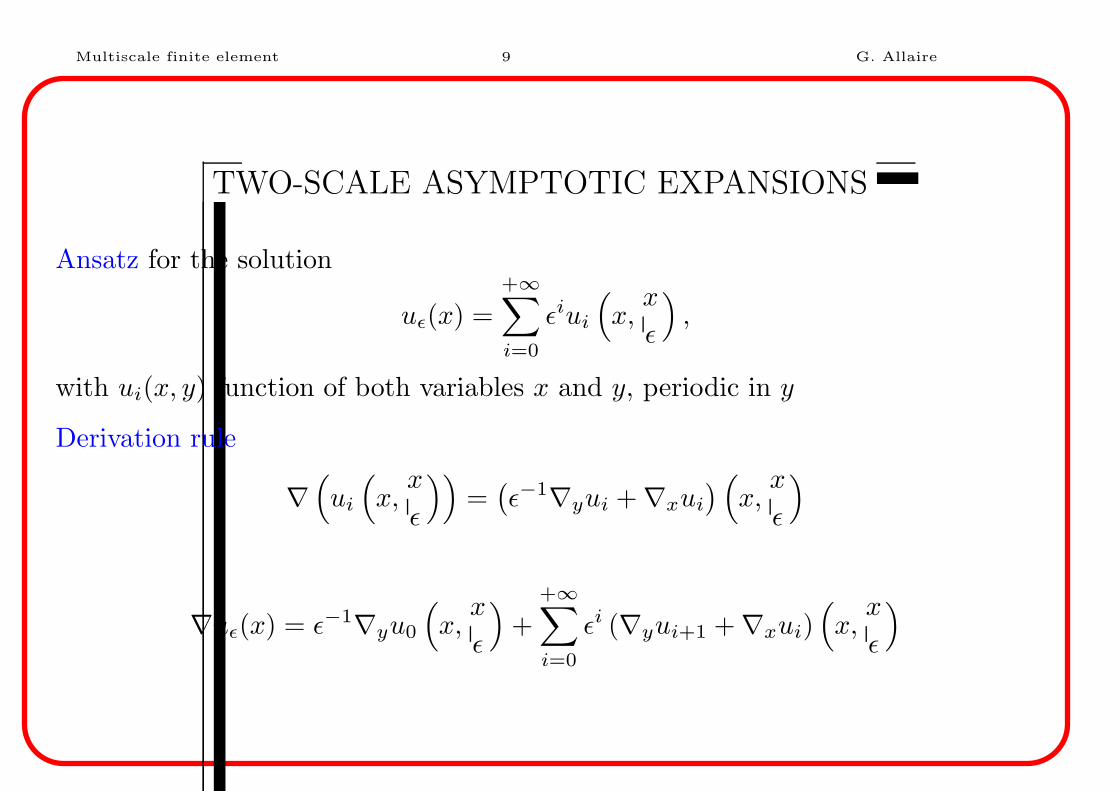
TWO-SCALE ASYMPTOTIC EXPANSIONS

Ansatz for the solution

uε(x) =+∞∑

i=0

εiui

(

x,x

ε

)

,

with ui(x, y) function of both variables x and y, periodic in y

Derivation rule

∇(

ui

(

x,x

ε

))

=(

ε−1∇yui + ∇xui

)

(

x,x

ε

)

∇uε(x) = ε−1∇yu0

(

x,x

ε

)

++∞∑

i=0

εi (∇yui+1 + ∇xui)(

x,x

ε

)


CASCADE OF EQUATIONS

−ε−2 [divy A∇yu0](

x,x

ε

)

−ε−1 [divy A(∇xu0 + ∇yu1) + divx A∇yu0](

x,x

ε

)

−ε0 [divx A(∇xu0 + ∇yu1) + divy A(∇xu1 + ∇yu2)](

x,x

ε

)

−+∞∑

i=1

εi [divx A(∇xui + ∇yui+1) + divy A(∇xui+1 + ∇yui+2)](

x,x

ε

)

= f(x).


εi equation

−divy (A(y)∇yui+2(x, y)) = f (ui, ui+1) (x, y) in Y

This is a partial differential equation in y.

We supplement it with periodic boundary conditions.

The macroscopic variable x is just a parameter.


Technical lemma on cell problems

Definition.

L2#(Y ) =

φ(y) Y -periodic, such that

∫

Y

φ(y)2dy < +∞

H1#(Y ) =

φ ∈ L2#(Y ) such that ∇φ ∈ L2

#(Y )N

Lemma. Let f(y) ∈ L2#(Y ) be a periodic function. There exists a solution in

H1#(Y ) (unique up to an additive constant) of

−div (A(y)∇w(y)) = f in Y

y → w(y) Y -periodic,

if and only if∫

Yf(y)dy = 0 (this is called the Fredholm alternative).


ε−2 equation

−divy (A(y)∇yu0(x, y)) = 0 in Y

where x is just a parameter.

Its unique solution does not depend on y

u0(x, y) ≡ u(x)


ε−1 equation

−divy A(y)∇yu1(x, y) = divy A(y)∇xu(x) in Y

which is an equation for u1. Introducing the cell problem

−divy A(y) (ei + ∇ywi(y)) = 0 in Y

y → wi(y) Y -periodic,

by linearity we compute

u1(x, y) =

N∑

i=1

∂u

∂xi(x)wi(y).


ε0 equation

−divy A(y)∇yu2(x, y) = divy A(y)∇xu1 + divx A(y) (∇yu1 + ∇xu) + f(x)

which is an equation for u2. Its compatibility condition (Fredholm alternative) is∫

Y

(divy A(y)∇xu1 + divx A(y) (∇yu1 + ∇xu) + f(x)) dy = 0.

Replacing u1 by its value yields the homogenized equation

−divx A∗∇xu(x) = f(x) in Ω

u = 0 on ∂Ω,

with the constant homogenized tensor

A∗ij =

∫

Y

[(A(y)∇ywi) · ej +Aij(y)] dy =

∫

Y

A(y) (ei + ∇ywi) · (ej + ∇wj) dy.


COMMENTS

Explicit formula for the effective parameters (no longer true for non-periodic

problems).

A∗ does not depend on ε, f , u or the boundary conditions (still true in the

non-periodic case).

A∗ is positive definite (not necessarily isotropic even if A(y) was so).

One can check that

limε→0

uε = u, limε→0

∇uε = ∇u, limε→0

A(x

ε

)

∇uε = A∗∇u,

limε→0

A(x

ε

)

∇uε · ∇uε = A∗∇u · ∇u.

Same results for evolution problems.

Very general method, but heuristic and not rigorous.


CONVERGENCE

Theorem.

uε(x) = u(x) + ε

N∑

i=1

∂u

∂xi(x)wi

(x

ε

)

+ rε(x) with ‖rε‖H1(Ω) ≤ C√ε

In particular, it implies∥

∥

∥

∥

∥

∇uε(x) −∇u(x) −N∑

i=1

∂u

∂xi(x)(∇ywi)

(x

ε

)

∥

∥

∥

∥

∥

L2(Ω)N

≤ C√ε

Correctors are important for the gradient.

We could have expected ‖rε‖H1(Ω) ≤ Cε and ‖rε‖L2(Ω) ≤ Cε2, but this is not

true in general.

”Bad estimates” are due to boundary layers effects.

Generalization to the non-periodic case.


HARMONIC VARIABLES (S. Kozlov)

uε(x) ≈ u(x) + ε

N∑

i=1

∂u

∂xi(x)wi

(x

ε

)

This ansatz looks like a Taylor expansion.

Corollary. Assume u ∈W 2,∞(Ω). Define w = (w1, ..., wN ). Then

uε(x) = u(

x+ εw(x

ε

))

+ sε(x) with ‖sε‖H1(Ω) ≤ C√ε.

(There is a generalization to the non-periodic case.)

Remark. In 2-d, x→(

x+ εw(

xε

))

is a change of variables (cf. Nesi).


-II- CLASSICAL FINITE ELEMENT METHODS

Stationary diffusion equation

−div (A(x)∇u) = f in Ω

u = 0 on ∂Ω

Sobolev space

H10 (Ω) =

φ such that

∫

Ω

(

φ2 + |∇φ|2)

dx < +∞ and φ = 0 on ∂Ω

Variational formulation: find u ∈ H10 (Ω) such that

∫

Ω

A(x)∇u · ∇φ dx =

∫

Ω

fφ dx ∀φ ∈ H10 (Ω)


Galerkin method for a finite dimensional subspace Vh ⊂ H10 (Ω): find an

approximate solution uh ∈ Vh such that∫

Ω

A(x)∇uh · ∇φh dx =

∫

Ω

fφh dx ∀φh ∈ Vh

Let (φj)1≤j≤ndlbe a basis of Vh and write uh =

ndl∑

j=1

Ujφj to get

ndl∑

j=1

Uj

∫

Ω

A(x)∇φj · ∇φi dx =

∫

Ω

fφi dx

Introducing

Kh =

(∫

Ω

A(x)∇φj · ∇φi dx

)

1≤i,j≤ndl

, and b =

(∫

Ω

fφi dx

)

1≤i≤ndl

we have to solve a linear system in IRndl

KhU = b


Typically Vh is associated to a mesh.

Example: P1 Lagrange finite elements.

xi

Basis function: φi affine on each (triangular) cell, equal to 1 on the node xi and 0

on all others nodes.

uh(x) =

ndl∑

i=1

Uiφi(x) ⇒ Ui = uh(xi)


Convergence

Theorem. For a sequence of ”uniformly regular” meshes in 2-d or 3-d, there

exists a constant C, independent of h and u such that

‖u− uh‖H1(Ω) ≤ Ch‖u‖H2(Ω)

(roughly, ‖u‖H2(Ω) ≈ ‖∇∇u‖L2(Ω))

Remark. In the case of oscillating coefficients A(

xε

)

, we have

uε(x) ≈ u(x) + ε

N∑

i=1

∂u

∂xi(x)wi

(x

ε

)

⇒ ‖uε‖H2(Ω) ≈ ε−1

so the P1 Finite Element method can converge only if h << ε.


Ingredients of the convergence proof

Cea’s lemma. Let u be the exact solution and uh the approximate one in Vh.

Then

‖u− uh‖H1(Ω) ≤ C infvh∈Vh

‖u− vh‖.

Interpolation lemma (P1 FEM in 2-d or 3-d). For any function v ∈ H2(Ω)

define its interpolate in Vh

rhv(x) =

ndl∑

i=1

v(xi)φi(x)

There exists a constant C, independent of h and v such that

‖v − rhv‖H1(Ω) ≤ Ch‖v‖H2(Ω).

Remark. For a multiscale finite element methods we must improve the

interpolation lemma by changing the basis functions.


-IV- MULTISCALE FINITE ELEMENT METHODS

Model problem

−div (Aε(x)∇uε) = f in Ω

uε = 0 on ∂Ω

Macro/micro approach: use a coarse mesh for defining the nodal values of uε

and a fine mesh for computing the basis functions φεi .

We pre-compute locally oscillating basis functions φεi that depend on Aε.

The problem dimension is that of the coarse mesh.

Multiscale FEM are defined for non-periodic problems but their quantitative

convergence analysis is made in the periodic case.

There are other problems and other methods...

Main references for this example: Hou, Efendiev, Wu, Babuska, Matache,

Schwab, Brizzi...


COARSE AND FINE MESHES

1

0

0


Multiscale Finite Element Method of T. Hou

xi

For each coarse triangle K, there is a fine mesh on which we compute φεi solution

of

−div (Aε∇φεi) = 0 in K

φεi(xj) = δij at the nodes of K

φεi(x) affine on ∂K


Multiscale Finite Element Method of T. Hou (continued)

By definition, the function φεi is continuous across cell boundaries ∂K.

This yields a conformal F.E.M.

The F.E. basis functions φεi encodes the oscillations of Aε.

Idea similar to the famous oscillating test function method of Tartar in

homogenization theory.

The computation of all φεi can be done in parallel (once and for all).

The previous definition is similar to the cell problem: if e · x is the affine

boundary condition, then wεi = φε

i − e · x satisfies

−div (Aε(e+ ∇wεi )) = 0 in K

wεi = 0 on ∂K


Convergence of the method (in the periodic case)

Theorem. Let uε be the exact solution and uhε the computed solution by the

multiscale FEM. Then

‖uε − uhε ‖H1(Ω) ≤ C

(

ε+ h+

√

ε

h

)

.

The classical finite element method does not converge if h >> ε.

Resonance effect when h ≈ ε for the multiscale FEM.

Although we analyze the convergence of the FEM in the periodic case, it is

well defined for non-periodic problems.


Sketch of the proof

Denoting by V εh the finite dimensional space spanned by the (φε

i), Cea’s lemma

implies

‖uε − uhε ‖H1(Ω) ≤ C inf

vhε∈ V ε

h

‖uε − vhε ‖H1(Ω).

We choose vhε = Πε

hu where u is the homogenized solution and Πεh is the

interpolation operator defined by

(Πεhv)(x) =

∑

i

v(xi)φεi(x)

On the other hand, using the homogenization ansatz


(

‖uε − u− εuε1‖H1(Ω) + ‖u+ εuε

1 − Πεhu‖H1(Ω)

)

≤ C(√ε+ ‖u+ εuε

1 − Πεhu‖H1(Ω)

)


Then using the homogenization ansatz for the basis function φεi on each coarse

cell K∥

∥

∥

∥

∥

φεi − φi − ε

d∑

k=1

wk

(x

ε

) ∂φi

∂xk

∥

∥

∥

∥

∥

H1(K)

≤ C

√

ε

h

√

|K|

where C is independent of h (the size of K).

This implies

‖u+εuε1−Πε

hu‖H1(Ω) ≤ C

(√

ε

h+ ‖u− Πhu‖H1(Ω) + ε‖w

(x

ε

)

∇(u− Πhu)‖H1(Ω)

)

where Πh is the usual interpolation operator on the coarse mesh. Recall that

‖u− Πhu‖H1(Ω) ≤ Ch‖u‖H2(Ω)

which yields the result.


Another multiscale method (Allaire-Brizzi)

Based on the harmonic variables of Kozlov

uε(x) ≈ u(

x+ εw(x

ε

))

with w = (w1, ..., wN ) solutions of the cell problems.

New idea: to compute an approximation of uε we use a standard finite element

method for u composed with the map x→(

x+ εw(

xε

))

.


INGREDIENTS

As many other methods we use a coarse mesh for u and a fine mesh for w.

On the coarse mesh: standard Pk F.E.M. with basis functions (φi) (of any

order k ≥ 1).

On the fine mesh: for each coarse triangle K we compute a locally oscillating

function χε solution of

−div(

A(

xε

)

∇χε)

= 0 in K

χε(x) = x on ∂K

Typically χε(x) ≈ x+ εw(

xε

)

.

Definition of the multiscale FEM: basis functions φεi(x) = φi χε(x).


CONVERGENCE (in the periodic case)

Theorem. If uhε is the approximated solution in the subspace spanned by

(φεi = φi χε), then


(

hk +

√

ε

h

)

.

If the oscillating functions χε are computed with a Pk′ FEM on the fine mesh of

size h′, then


(

hk +

√

ε

h+

(

h′

ε

)k′)

.


Idea of the proof

By Cea’s lemma

‖uε − uhε ‖H1(Ω) ≤ C inf

vhε∈ V ε

h

‖uε − vhε ‖H1(Ω).

We choose vhε = (Πhu) χε where Πh is the usual interpolation operator on the

coarse mesh. Then


(

‖uε − u χε‖H1(Ω) + ‖(u− Πhu) χε‖H1(Ω)

)

.

(But this estimate has to be done on each coarse cell K.)

A standard computation yields the result.


REMARKS

Each oscillating function χε is computed independently of the others (natural

parallelism).

The complexity of the macroscopic computation is linked to the coarse mesh.

No periodicity is required.

When k = 1, we recover exactly the previous method of Hou et al.

We perform numerical experiments for k = 2.

One can choose a larger support for χε (over-sampling in order to avoid

boundary layer effects) and still have a conforming F.E.M.

Our method works in any dimension and for any type of mesh.


SOME IMPROVEMENTS

The error estimate in√

ε/h indicates a resonance effect.

It is due to boundary layers.

It cannot be removed completely but some ideas are helpful.

First idea: Replace the affine boundary conditions on ∂K for φεi by oscillating

boundary conditions: for example, in 2-d

−div (Aε(x)∇φεi) = 0 in K,

φεi = bεi(x) on ∂K,

where on each side of ∂K, parametrized by a curvilinear coordinate s ∈ [0, 1],

− d

ds

(

Aε d bε,Ki

ds

)

= 0

with the boundary conditions bεi(x(0)) = xi(0) and bεi(x(1)) = xi(1).


Second idea: Oversampling method (T. Hou)

K

K

’

Oversampling method: compute φεi on a larger fine mesh K ′ such that K ⊂⊂ K ′

(overlap).

Non-conforming F.E. method with a better convergence rate


(

h+ ε+ε

h

)


NUMERICAL EXPERIMENTS

Test proposed by T. Hou in the 2-D periodic case

A(y) =1

(2 + 1.8 sin(2πy1))(2 + 1.8 sin(2πy2)).

Method of Allaire-Brizzi with P2 F.E.

A∗ = 1/(2√

4 − (1.8)2)

constant source term f = −1

Ω = (0, 1)2 with Dirichlet boundary conditions

ε = 0.01

coarse triangular mesh with h = 1/5

fine triangular mesh with h′ = 4.10−4


x

U_e

ps(x

,y=0

.5)

0 10.5

-0.1

0

-0.05

P2-MSFEM P1-FEM reference

x

U_e

ps(x

,y=0

.5)

0.2 0.21 0.22 0.23 0.24 0.25

-0.1

-0.09

-0.08

P2-MSFEM P1-FEM reference

Cross section (left) and close-up (right) at y = 0.5 of the reference and multiscale

solutions: ε = 10−2, h = 1/5, h′ = 4.10−4


x

DU

eps/

Dx(

x,y=

0.5)

0 10.5

-1

0

1

-0.5

0.5

P2-MsFEMP1-FEM H

x

DU

eps/

Dx(

x,y=

0.5)

0.28 0.29 0.3 0.31 0.32 0.33 0.34

-0.4

-0.3

-0.2

-0.1

0

P2-MsFEM P1-FEM referenceH*

Cross-section (left) and close-up (right) of the partial derivative ∂uε/∂x at

y = 0.5 of the reference and multiscale solutions: ε = 10−2, h = 1/5, h′ = 4.10−4.

Here, H stands for the homogenized solution.


Predicted error estimate when k = 2, k′ = 1

gε(h) = h2 +

√

ε

h+h′

ε.

If we assume that h′ is very small compare to ε, the optimal mesh size is

h ' ε1/5.


h

g_ep

s(h)

0 0.1 0.2 0.3 0.4 0.50.1

0.3

0.5

0.7

0.9 EPS = 0.01EPS = 0.02EPS = 0.04EPS = 0.08

h

||Uep

s,h

- U

ref||

H1

0.1 0.2 0.3 0.4 0.5

0.1

0.05

0.15

EPS = 0.08EPS = 0.04EPS = 0.02EPS = 0.01

Error estimate (in the H1 norm) predicted by the previous formula (left) and

computed (right) as a function of h for different values of ε with h′ = 4. 10−4.


h ‖ uεh − uε ‖L2(Ω) ‖ uε

h − uε ‖H1

0(Ω) ‖ uε

h − uε ‖L∞(Ω)

0.0666 0.372 E-02 0.721 E-01 0.673 E-02

0.0769 0.327 E-02 0.685 E-01 0.792 E-01

0.0833 0.287 E-02 0.654 E-01 0.522 E-02

0.1000 0.105 E-03 0.583 E-01 0.196 E-02

0.1250 0.146 E-02 0.557 E-01 0.273 E-02

0.1666 0.116 E-02 0.517 E-01 0.313 E-02

0.2000 0.412 E-03 0.491 E-01 0.243 E-02

0.2500 0.702 E-03 0.509 E-01 0.405 E-02

0.3333 0.195 E-02 0.600 E-01 0.604 E-02

0.5000 0.536 E-02 0.926 E-01 0.107 E-01

Error estimates (in various norms) as a function of h for ε = 10−2 and

h′ = 4. 10−4.


h N CPU1 (s) CPU2 (s) CPU1/N (s)

0.0666 450 81918 1.05 182

0.0769 338 65508 0.46 193

0.1000 200 47520 0.11 237

0.1250 128 25640 0.04 200

0.2000 50 9897 0.01 197

0.2500 32 6367 0.01 198

0.3333 18 3619 0.01 201

0.5000 8 1849 0.01 231

CPU times (in seconds). N is the total number of elements in the coarse mesh.

CPU1 is the total sequential time for computing the oscillating functions wε,h

(thus CPU1/N is the corresponding parallel time ). CPU2 is the inherently

sequential time for the coarse mesh computation (assembling and solving).


P1 multiscale FEM P2 multiscale FEM

h ‖uεh − uε‖L2(Ω) ‖uε

h − uε‖H1(Ω) ‖uεh − uε‖L2(Ω) ‖uε

h − uε‖H1(Ω)

0.0666 0.442E-02 0.828E-01 0.346E-02 0.714E-01

0.1000 0.289E-02 0.840E-01 0.955E-03 0.581E-01

0.1250 0.415E-02 0.921E-01 0.131E-02 0.547E-01

0.2000 0.676E-02 0.117E+00 0.412E-03 0.491E-01

0.2500 0.929E-02 0.134E+00 0.702E-03 0.509E-01

0.3333 0.133E-01 0.154E+00 0.195E-02 0.600E-01

0.5000 0.155E-01 0.168E+00 0.536E-02 0.926E-01

Comparison P1 (left) and P2 (right): error estimates (in various norms) as a

function of h for ε = 10−2 and h′ = h/500.


2-d non-periodic problem

Discontinuous coefficients:

Aε(x) =

1 in the matrix

100 in the inclusions

106 monodisperse spherical inclusions in a matrix.

Domain Ω = (0, 1)2, without source term.

Boundary conditions: Neumann on the vertical sides, Dirichlet 0 (bottom) and 1

(top).


Γ1

Γ1

Γ0

Γ0

(a) (b)

Coarse mesh. Close-up on the inclusions.


Flux density |Aε∇uε| in a coarse mesh cell and close-up.


y

DU

_eps

/Dy(

x=0.

5,y)

0.49 0.5 0.510.495 0.505 0.515

0

1

2

0.5

1.5

P2-MsFEM

Close-up of the vertical cross-sections of the partial derivative ∂uε/∂y(x = 0.5, y).


y

DU

_eps

/Dx(

x=0.

5,y)

0.49 0.5 0.510.495 0.505 0.515

-1

0

-0.5

0.5

P2-MsFEM

Close-up of the vertical cross-sections of the partial derivative ∂uε/∂x(x = 0.5, y).


-V- ANOTHER HOMOGENIZATION PARADIGM

Different model problem and diferent scaling.

A diferent homogenization paradigm yields a different multiscale method.

Previously the solution was behaving like

uε(x) ≈ u(x) + εu1

(

x,x

ε

)

,

Now we want to have large oscillations in the leading term

uε(x) ≈ u0

(

x,x

ε

)

+ εu1

(

x,x

ε

)

,

Such a model can be found in neutronic diffusion, radiative transport,

semiconductors...


Example: neutronic diffusion model

c(x

ε

) ∂uε

∂t− ε2div

(

A(x

ε

)

uε

)

= σ(x

ε

)

uε in Ω

uε = 0 on ∂Ω

uε(0) = u0

uε(t, x) ≈ e−λtw(x

ε

)

u(

ε2t, x)

−λc(y)w − div (A(y)w) = σ(y)w in Y

y → w(y) Y − periodic

c∗∂u

∂τ− div

(

A∗u)

= 0 in Ω

u = 0 on ∂Ω

u(0) = u0


Two groups neutronic diffusion computation (Allaire and Siess)


HYDRODYNAMIC LIMIT OF KINETIC EQUATION

Transport or kinetic equation: particle density φ(x, v) in Ω × V

∂φε

∂t+ εv · ∇φε =

∫

V

σ(x

ε, v′, v

)

φε(x, v′)dv′ − Σ

(x

ε, v)

φε(x, v)

φε = 0 on Γ− = (x, v) ∈ ∂Ω × V | v · n(x) < 0,

Singular perturbations: mean free path of the order of ε, characteristic time

of observation of the order of 1/ε2.

Hydrodynamic or fluid limit: change of type of the equations.

Origin of the scaling: change of variables y = x/ε ⇒ cells of size 1, domain

of size 1/ε, no more ε in the equations.


CONVERGENCE RESULT

φε(t, x, v) ≈ e−λtψ(x

ε, v)

u(

ε2t, x)

Spectral cell problem:

−λψ + v · ∇yψ =

∫

V

σ (y, v′, v)ψ(y, v′)dv′ − Σ (y, v)ψ(y, v) in Y

y → ψ(y, v) Y − periodic

First eigenvalue λ and first eigenfunction ψ(y, v) > 0 (local equilibrium between

transport and scattering).

Change of unknown: uε(ε2t, x, v) =

φε(t, x, v)

ψ(

xε , v) eλt


Homogenized problem for uε:

c∗∂u

∂τ− div (A∗∇u) = 0 in Ω

u = 0 on ∂Ω

u(0) = u0

Conclusion: microscopic transport equation, homogenized diffusion equation.

At the basis of many numerical methods.

Complicated but explicit formula for c∗ and A∗.

Boundary layers are very important.

Many contributions: Keller, Larsen, Bensoussan-Lions-Papanicolaou, Sentis,

Allaire-Bal...


0

0.1

0.2

0.3

0.4

0.5

0.6

0.7

0.8

0.9

1

1.1

0 20 40 60 80 100

’Reconstructed Flux’’Reference Flux’


A short list of references

Homogenization theory:

Bensoussan, A.; Lions, J.-L.; Papanicolaou, G.; Asymptotic analysis for periodic

structures; North-Holland: Amsterdam, 1978.

Jikov, V. V.; Kozlov, S. M.; Oleinik, O. A.; Homogenization of Differential Operators

and Integral Functionals; Springer Verlag: New York, Berlin, 1994.

Multiscale finite element methods:

T. Hou, X.-H. Wu, A multiscale finite element method for elliptic problems in composite

materials and porous media, J.Comput.Phys. 134, pp.169-189 (1997).

W. E, B. Engquist, The heterogeneous multiscale methods, Commun. Math. Sci. 1,

87–132 (2003).

A.-M. Matache, I. Babuska, C. Schwab, Generalized p-FEM in homogenization, Numer.

Math. 86, 319–375 (2000).


T. Arbogast, Numerical subgrid upscaling of two-phase flow in porous media, in

Numerical treatment of multiphase flows in porous media, Lecture Notes in Physics,

vol. 552, Chen, Ewing and Shi eds., pp.35-49 (2000).

Homogenization of transport equations:

G. Allaire, G. Bal, Homogenization of the criticality spectral equation in neutron

transport, M2AN 33, pp.721-746 (1999).

AN INTRODUCTION TO MULTISCALE FINITE ELEMENT …allaire/multimat/allaire_lecture.pdf · Multiscale...

Documents

Transcript of AN INTRODUCTION TO MULTISCALE FINITE ELEMENT …allaire/multimat/allaire_lecture.pdf · Multiscale...