
An Introduction to Dynamics of Structures - boffi.github.io · Dynamics of Structures Giacomo Bo...
19
Dynamics of Structures Giacomo Boffi An Introduction to Dynamics of Structures Giacomo Boffi http://intranet.dica.polimi.it/people/boffi-giacomo Dipartimento di Ingegneria Civile Ambientale e Territoriale Politecnico di Milano February 27, 2018 Dynamics of Structures Giacomo Boffi Outline Part 1 Introduction Characteristics of a Dynamical Problem Formulation of a Dynamical Problem Formulation of the equations of motion Part 2 1 DOF System Free vibrations of a SDOF system Free vibrations of a damped system Dynamics of Structures Giacomo Boffi Introduction Characteristics of a Dynamical Problem Formulation of a Dynamical Problem Formulation of the equations of motion Definitions Let’s start with some definitions Dynamic adj., constantly changing Dynamics noun, the branch of Mechanics concerned with the motion of bodies under the action of forces Dynamic Loading a Loading that varies over time Dynamic Response the Response (deflections and stresses) of a system to a dynamic loading; Dynamic Responses vary over time Dynamics of Structures all of the above, applied to a structural system, i.e., a system designed to stay in equilibrium
Transcript of An Introduction to Dynamics of Structures - boffi.github.io · Dynamics of Structures Giacomo Bo...

Dynamics ofStructures
Giacomo Boffi
An Introduction to Dynamics of Structures
Giacomo Boffi
http://intranet.dica.polimi.it/people/boffi-giacomo
Dipartimento di Ingegneria Civile Ambientale e TerritorialePolitecnico di Milano
February 27, 2018
Dynamics ofStructures
Giacomo Boffi
Outline
Part 1Introduction
Characteristics of a Dynamical Problem
Formulation of a Dynamical Problem
Formulation of the equations of motion
Part 2
1 DOF System
Free vibrations of a SDOF system
Free vibrations of a damped system
Dynamics ofStructures
Giacomo Boffi
Introduction
Characteristics ofa DynamicalProblem
Formulation of aDynamicalProblem
Formulation ofthe equations ofmotion
Definitions
Let’s start with some definitionsDynamic adj., constantly changingDynamics noun, the branch of Mechanics concerned with
the motion of bodies under the action of forcesDynamic Loading a Loading that varies over time
Dynamic Response the Response (deflections and stresses) of asystem to a dynamic loading; DynamicResponses vary over time
Dynamics of Structures all of the above, applied to a structuralsystem, i.e., a system designed to stay inequilibrium

Dynamics ofStructures
Giacomo Boffi
Introduction
Characteristics ofa DynamicalProblem
Formulation of aDynamicalProblem
Formulation ofthe equations ofmotion
Dynamics of Structures
Our aim is to determine the stresses and deflections that a dynamicloading induces in a structure that remains in the neighborhood of apoint of equilibrium.
Methods of dynamic analysis are extensions of the methods ofstandard static analysis, or to say it better, static analysis is indeed aspecial case of dynamic analysis.
If we restrict ourselves to analysis of linear systems, it is soconvenient to use the principle of superposition to study the com-bined effects of static and dynamic loadings that different meth-ods, of different character, are applied to these different loadings.
Dynamics ofStructures
Giacomo Boffi
Introduction
Characteristics ofa DynamicalProblem
Formulation of aDynamicalProblem
Formulation ofthe equations ofmotion
Types of Dynamic Analysis
Taking into account linear systems only, we must consider twodifferent definitions of the loading to define two types of dynamicanalysisDeterministic Analysis applies when the time variation of the loading
is fully known and we can determine the complete timevariation of all the required response quantities
Non-deterministic Analysis applies when the time variation of theloading is essentially random and is known only interms of some statisticsIn a non-deterministic or stochastic analysis thestructural response can be known only in terms ofstatistics of the response quantities
Our focus will be on deterministic analysis
Dynamics ofStructures
Giacomo Boffi
Introduction
Characteristics ofa DynamicalProblem
Formulation of aDynamicalProblem
Formulation ofthe equations ofmotion
Types of Dynamic Loading
Dealing with deterministic dynamic loadings we will study, in order ofcomplexity,
Harmonic Loadings a force is modulated by a harmonic function of time,characterized by a frequency ω and a phase ϕ:
p(t) = p0 sin(ωt − ϕ)
Periodic Loadings a periodic loading repeats itself with a fixed period T :
p(t) = p0 f (t) with f (t) ≡ f (t + T )
Non Periodic Loadings here we see two sub-cases,I the loading can be described in terms of an analytical
function, e.g.,
p(t) = po exp(αt)
I the loading is measured experimentally, hence it isknown only in a discrete set of instants; in this case,we say that we know the loading time-history.

Dynamics ofStructures
Giacomo Boffi
Introduction
Characteristics ofa DynamicalProblem
Formulation of aDynamicalProblem
Formulation ofthe equations ofmotion
Characteristics of a Dynamical Problem
A dynamical problem is essentially characterized by the relevance ofinertial forces, arising from the accelerated motion of structural orserviced masses.
A dynamic analysis is required only when the inertial forces representa significant portion of the total load.
On the other hand, if the loads and the deflections are varyingslowly, a static analysis will provide an acceptable approximation.
We will define slowly
Dynamics ofStructures
Giacomo Boffi
Introduction
Characteristics ofa DynamicalProblem
Formulation of aDynamicalProblem
Formulation ofthe equations ofmotion
Formulation of a Dynamical Problem
In a structural system the inertial forces depend on the timederivatives of displacements while the elastic forces, equilibrating theinertial ones, depend on the spatial derivatives of the displacements.... the natural statement of the problem is hence in terms of partialdifferential equations.
In many cases it is however possible to simplify the formulation ofthe structural dynamic problem to ordinary differential equations.
Dynamics ofStructures
Giacomo Boffi
Introduction
Characteristics ofa DynamicalProblem
Formulation of aDynamicalProblem
Formulation ofthe equations ofmotion
Lumped Masses
In many structural problems we can say that the masses areconcentrated in a discrete set of lumped masses (e.g., in a multi-storeybuilding most of the masses is concentrated at the level of thestoreys’floors).Under this assumption, the analytical problem is greatly simplified:1. the inertial forces are applied only at the lumped masses,2. the only deflections that influence the inertial forces are the
deflections of the lumped masses,3. using methods of static analysis we can determine those
deflections,thus consenting the formulation of the problem in terms of a set ofordinary differential equations, one for each relevant component ofthe inertial forces.

Dynamics ofStructures
Giacomo Boffi
Introduction
Characteristics ofa DynamicalProblem
Formulation of aDynamicalProblem
Formulation ofthe equations ofmotion
Dynamic Degrees of Freedom
The dynamic degrees of freedom (DDOF) in a discretized system arethe displacements components of the lumped masses associated withthe relevant components of the inertial forces.If a lumped mass can be regarded as a point mass then at most 3translational DDOFs will suffice to represent the associated inertialforce.On the contrary, if a lumped mass has a discrete volume its inertialforce depends also on its rotations (inertial couples) and we need atmost 6 DDOFs to represent the mass deflections and the inertialforce.
Of course, a continuous system has an infinite number of degrees offreedom.
Dynamics ofStructures
Giacomo Boffi
Introduction
Characteristics ofa DynamicalProblem
Formulation of aDynamicalProblem
Formulation ofthe equations ofmotion
Generalized Displacements
The lumped mass procedure that we have outlined is effective if alarge proportion of the total mass is concentrated in a few points(e.g., in a multi-storey building one can consider a lumped mass foreach storey).When the masses are distributed we can simplify our problemexpressing the deflections in terms of a linear combination of assignedfunctions of position, the coefficients of the linear combination beingthe generalized coordinates (e..g., the deflections of a rectilinearbeam can be expressed in terms of a trigonometric series).
Dynamics ofStructures
Giacomo Boffi
Introduction
Characteristics ofa DynamicalProblem
Formulation of aDynamicalProblem
Formulation ofthe equations ofmotion
Generalized Displacements, cont.
To fully describe a displacement field, we need to combine an infinityof linearly independent base functions, but in practice a goodapproximation can be achieved using just a small number offunctions and degrees of freedom.
Even if the method of generalized coordinates has itsbeauty, we must recognize that for each different problemwe have to derive an ad hoc formulation, with an evidentloss of generality.

Dynamics ofStructures
Giacomo Boffi
Introduction
Characteristics ofa DynamicalProblem
Formulation of aDynamicalProblem
Formulation ofthe equations ofmotion
Finite Element Method
The finite elements method (FEM) combines aspects of lumpedmass and generalized coordinates methods, providing a simple andreliable method of analysis, that can be easily programmed on adigital computer.
Dynamics ofStructures
Giacomo Boffi
Introduction
Characteristics ofa DynamicalProblem
Formulation of aDynamicalProblem
Formulation ofthe equations ofmotion
Finite Element Method
I In the FEM, the structure is subdivided in a number ofnon-overlapping pieces, called the finite elements, delimited bycommon nodes.
I The FEM uses piecewise approximations (i.e., local to eachelement) to the field of displacements.
I In each element the displacement field is derived from thedisplacements of the nodes that surround each particularelement, using interpolating functions.
I The displacement, deformation and stress fields in eachelement, as well as the inertial forces, can thus be expressed interms of the unknown nodal displacements.
I The nodal displacements are the dynamical DOFs of the FEMmodel.
Dynamics ofStructures
Giacomo Boffi
Introduction
Characteristics ofa DynamicalProblem
Formulation of aDynamicalProblem
Formulation ofthe equations ofmotion
Finite Element Method
Some of the most prominent advantages of the FEM method are1. The desired level of approximation can be achieved by further
subdividing the structure.2. The resulting equations are only loosely coupled, leading to an
easier computer solution.3. For a particular type of finite element (e.g., beam, solid, etc)
the procedure to derive the displacement field and the elementcharacteristics does not depend on the particular geometry ofthe elements, and can easily be implemented in a computerprogram.
Dynamics ofStructures
Giacomo Boffi
Introduction
Characteristics ofa DynamicalProblem
Formulation of aDynamicalProblem
Formulation ofthe equations ofmotion
Writing the equation of motion
In a deterministic dynamic analysis, given a prescribed load, we wantto evaluate the displacements in each instant of time.In many cases a limited number of DDOFs gives a sufficientaccuracy; further, the dynamic problem can be reduced to thedetermination of the time-histories of some selected component ofthe response.The mathematical expressions, ordinary or partial differentialequations, that we are going to write express the dynamicequilibrium of the structural system and are known as the Equationsof Motion (EOM).The solution of the EOM gives the requested displacements.The formulation of the EOM is the most important, often the mostdifficult part of a dynamic analysis.
Dynamics ofStructures
Giacomo Boffi
Introduction
Characteristics ofa DynamicalProblem
Formulation of aDynamicalProblem
Formulation ofthe equations ofmotion
Writing the EOM, cont.
We have a choice of techniques to help us in writing the EOM,namely:I the D’Alembert Principle,I the Principle of Virtual Displacements,I the Variational Approach.
Dynamics ofStructures
Giacomo Boffi
Introduction
Characteristics ofa DynamicalProblem
Formulation of aDynamicalProblem
Formulation ofthe equations ofmotion
D’Alembert principle
By Newton’s II law of motion, for any particle the rate of change ofmomentum is equal to the external force,
~p(t) =d
dt(m
d~u
dt),
where ~u(t) is the particle displacement.In structural dynamics, we may regard the mass as a constant, andthus write
~p(t) = m~u,
where each operation of differentiation with respect to time isdenoted with a dot.If we write
~p(t)−m~u = 0
and interpret the term −m~u as an Inertial Force that contrasts theacceleration of the particle, we have an equation of equilibrium forthe particle.

Dynamics ofStructures
Giacomo Boffi
Introduction
Characteristics ofa DynamicalProblem
Formulation of aDynamicalProblem
Formulation ofthe equations ofmotion
D’Alembert principle, cont.
The concept that a mass develops an inertial force opposing itsacceleration is known as the D’Alembert principle, and using thisprinciple we can write the EOM as a simple equation of equilibrium.The term ~p(t) must comprise each different force acting on theparticle, including the reactions of kinematic or elastic constraints,internal forces and external, autonomous forces.In many simple problems, D’Alembert principle is the most directand convenient method for the formulation of the EOM.
Dynamics ofStructures
Giacomo Boffi
Introduction
Characteristics ofa DynamicalProblem
Formulation of aDynamicalProblem
Formulation ofthe equations ofmotion
Principle of virtual displacements
In a reasonably complex dynamic system, with e.g. articulated rigidbodies and external/internal constraints, the direct formulation ofthe EOM using D’Alembert principle may result difficult.In these cases, application of the Principle of Virtual Displacementsis very convenient, because the reactive forces do not enter theequations of motion, that are directly written in terms of themotions compatible with the restraints/constraints of the system.
Dynamics ofStructures
Giacomo Boffi
Introduction
Characteristics ofa DynamicalProblem
Formulation of aDynamicalProblem
Formulation ofthe equations ofmotion
Principle of Virtual Displacements, cont.
For example, considering an assemblage of rigid bodies, the pvdstates that necessary and sufficient condition for equilibrium is that,for every virtual displacement (i.e., any infinitesimal displacementcompatible with the restraints) the total work done by all theexternal forces is zero.For an assemblage of rigid bodies, writing the EOM requires1. to identify all the external forces, comprising the inertial forces,
and to express their values in terms of the ddof;2. to compute the work done by these forces for different virtual
displacements, one for each ddof;3. to equate to zero all these work expressions.
The pvd is particularly convenient also because we have only scalarequations, even if the forces and displacements are of vectorialnature.

Dynamics ofStructures
Giacomo Boffi
Introduction
Characteristics ofa DynamicalProblem
Formulation of aDynamicalProblem
Formulation ofthe equations ofmotion
Variational approach
Variational approaches do not consider directly the forces acting onthe dynamic system, but are concerned with the variations of kineticand potential energy and lead, as well as the pvd, to a set of scalarequations.
For example, the equation of motion of a generical system can bederived in terms of the Lagrangian function, L = T − V where Tand V are, respectively, the kinetic and the potential energy of thesystem expressed in terms of a vector ~q of indipendent coordinates
d
dt
(∂L∂qi
)=∂L∂qi
, i = 1, . . . ,N.
The method to be used in a particular problem is mainly a matter ofconvenience (and, to some extent, of personal taste).
Dynamics ofStructures
Giacomo Boffi
1 DOF System
Free vibrations ofa SDOF system
Free vibrations ofa damped system
1 DOF System
Structural dynamics is all about the motion of a system in theneighborhood of a point of equilibrium.We’ll start by studying the most simple of systems, a single degree offreedom system, without external forces, subjected to a perturbationof the equilibrium.If our system has a constant mass m and it’s subjected to a generical,non-linear, internal force F = F (y , y), where y is the displacementand y the velocity of the particle, the equation of motion is
y =1mF (y , y) = f (y , y).
It is difficult to integrate the above equation in the general case, butit’s easy when the motion occurs in a small neighborhood of theequilibrium position.
Dynamics ofStructures
Giacomo Boffi
1 DOF System
Free vibrations ofa SDOF system
Free vibrations ofa damped system
1 DOF System, cont.
In a position of equilibrium, yeq., the velocity and the accelerationare zero, and hence f (yeq., 0) = 0.The force can be linearized in a neighborhood of yeq., 0:
f (y , y) = f (yeq., 0) +∂f
∂y(y − yeq.) +
∂f
∂y(y − 0) + O(y , y).
Assuming that O(y , y) is small in a neighborhood of yeq., we canwrite the equation of motion
x + ax + bx = 0
where x = y − yeq., a = − ∂f∂y
∣∣∣y=0
and b = − ∂f∂y
∣∣∣y=yeq
.
In an infinitesimal neighborhood of yeq., the equation of motion canbe studied in terms of a linear, constant coefficients differentialequation of second order.

Dynamics ofStructures
Giacomo Boffi
1 DOF System
Free vibrations ofa SDOF system
Free vibrations ofa damped system
1 DOF System, cont.
A linear constant coefficient differential equation has thehomogeneous integral x = A exp(st), that substituted in theequation of motion gives
s2 + as + b = 0
whose solutions are
s1,2 = −a
2∓√
a2
4− b.
The general integral is hence
x(t) = A1 exp(s1t) + A2 exp(s2t).
Dynamics ofStructures
Giacomo Boffi
1 DOF System
Free vibrations ofa SDOF system
Free vibrations ofa damped system
1 DOF System, cont.
Given that for a free vibration problem A1, A2 are given by the initialconditions, the nature of the solution depends on the sign of the realpart of s1, s2, because si = ri + ıqi and
exp(si t) = exp(ıqi t) exp(ri t).
If one of the ri > 0, the response grows infinitely over time, even foran infinitesimal perturbation of the equilibrium, so that in this casewe have an unstable equilibrium.If both ri < 0, the response decrease over time, so we have a stableequilibrium.Finally, if both ri = 0 the roots si are purely imaginary and theresponse is harmonic with constant amplitude.
Dynamics ofStructures
Giacomo Boffi
1 DOF System
Free vibrations ofa SDOF system
Free vibrations ofa damped system
1 DOF System, cont.
The roots being
s1,2 = −a
2∓√
a2
4− b,
I if a > 0 and b > 0 both roots are negative or complex conjugatewith negative real part, the system is asymptotically stable,
I if a = 0 and b > 0, the roots are purely imaginary, theequilibrium is indifferent, the oscillations are harmonic,
I if a < 0 or b < 0 at least one of the roots has a positive realpart, and the system is unstable.

Dynamics ofStructures
Giacomo Boffi
1 DOF System
Free vibrations ofa SDOF system
Free vibrations ofa damped system
The famous box car
In a single degree of freedom (sdof) system each property, m, a andb, can be conveniently represented in a single physical elementI The entire mass, m, is concentrated in a rigid block, its position
completely described by the coordinate x(t).I The energy-loss (the a x term) is represented by a massless
damper, its damping constant being c .I The elastic resistance to displacement (b x) is provided by a
massless spring of stiffness kI For completeness we consider also an external loading, the
time-varying force p(t).
(a)
m
c
k
p(t)
xx(t)
(b)
p(t)fD(t)
fS(t)
fI(t)
Dynamics ofStructures
Giacomo Boffi
1 DOF System
Free vibrations ofa SDOF system
Free vibrations ofa damped system
Equation of motion of the basic dynamic system
(a)
m
c
k
p(t)
xx(t)
(b)
p(t)fD(t)
fS(t)
fI(t)
The equation of motion can be written using the D’Alembert Principle,expressing the equilibrium of all the forces acting on the mass includingthe inertial force.The forces are the external force, p(t), positive in the direction of motionand the resisting forces, i.e., the inertial force fI(t), the damping forcefD(t) and the elastic force, fS(t), that are opposite to the direction of theacceleration, velocity and displacement.The equation of motion, merely expressing the equilibrium of these forces,writing the resisting forces and the external force across the equal sign
fI(t) + fD(t) + fS(t) = p(t)
Dynamics ofStructures
Giacomo Boffi
1 DOF System
Free vibrations ofa SDOF system
Free vibrations ofa damped system
EOM of the basic dynamic system, cont.
According to D’Alembert principle, the inertial force is the product ofthe mass and acceleration
fI(t) = m x(t).
Assuming a viscous damping mechanism, the damping force is theproduct of the damping constant c and the velocity,
fD(t) = c x(t).
Finally, the elastic force is the product of the elastic stiffness k andthe displacement,
fS(t) = k x(t).

Dynamics ofStructures
Giacomo Boffi
1 DOF System
Free vibrations ofa SDOF system
Free vibrations ofa damped system
EOM of the basic dynamic system, cont.
The differential equation of dynamic equilibrium
fI(t) + fD(t) + fS(t) =
m x(t) + c x(t) + k x(t) = p(t).
The resisting forces in the EoM
fI(t) + fD(t) + fS(t) = p(t)
are proportional to the deflection x(t) or one of its time derivatives,x(t), x(t).The equation of motion is a linear differential equation of the secondorder, with constant coefficients.The resisting forces are, by convention, positive when opposite to thedirection of motion, i.e., resisting the motion.
Dynamics ofStructures
Giacomo Boffi
1 DOF System
Free vibrations ofa SDOF system
Free vibrations ofa damped system
Influence of static forces
(a)
m
c
k
p(t)
x(t)x
∆st x(t)
(b)
p(t)
k∆st
fS(t)fD(t)
W
fI(t)
Considering the presence of a constant force W , the EOM is
m x(t) + c x(t) + k x(t) = p(t) + W .
Expressing the displacement as the sum of a constant, staticdisplacement and a dynamic displacement,
x(t) = ∆st + x(t),
and substituting in the EOM we have
m x(t) + c x(t) + k ∆st + k x(t) = p(t) + W .
Dynamics ofStructures
Giacomo Boffi
1 DOF System
Free vibrations ofa SDOF system
Free vibrations ofa damped system
Influence of static forces, cont.
Recognizing that k ∆st = W (so that the two terms, on oppositesides of the equal sign, cancel each other), that x ≡ ˙x and thatx ≡ ¨x the EOM can be written as
m ¨x(t) + c ˙x(t) + k x(t) = p(t).
The equation of motion expressed with reference to the staticequilibrium position is not affected by static forces.For this reasons, all displacements in further discussions will bereferenced from the equilibrium position and denoted, for simplicity,with x(t).
Note that the total displacements, stresses. etc. areinfluenced by the static forces, and must be computed usingthe superposition of effects.

Dynamics ofStructures
Giacomo Boffi
1 DOF System
Free vibrations ofa SDOF system
Free vibrations ofa damped system
Influence of support motion
Fixed
reference
axis
xtot(t)
xg(t) x(t)
k
2
k
2
m
c
Displacements, deformations and stresses in a structure are induced alsoby a motion of its support.Important examples of support motion are the motion of a buildingfoundation due to earthquake and the motion of the base of a piece ofequipment due to vibrations of the building in which it is housed.
Dynamics ofStructures
Giacomo Boffi
1 DOF System
Free vibrations ofa SDOF system
Free vibrations ofa damped system
Influence of support motion, cont.
Fixed
reference
axis
xtot(t)
xg(t) x(t)
k
2
k
2
m
c
Considering a support motion xg(t), definedwith respect to a inertial frame of reference,the total displacement is
xtot(t) = xg(t) + x(t)
and the total acceleration is
xtot(t) = xg(t) + x(t).
While the elastic and damping forces are still proportional to relativedisplacements and velocities, the inertial force is proportional to the totalacceleration,
fI(t) = −mxtot(t) = mxg(t) +mx(t).
Writing the EOM for a null external load, p(t) = 0, is hence
m xtot(t) + c x(t) + k x(t) = 0, or,
m x(t) + c x(t) + k x(t) = −m xg(t) ≡ peff(t).
Support motion is sufficient to excite a dynamic system: peff(t) = −m xg(t).
Dynamics ofStructures
Giacomo Boffi
1 DOF System
Free vibrations ofa SDOF system
Free vibrations ofa damped system
Free Vibrations
The equation of motion,
m x(t) + c x(t) + k x(t) = p(t)
is a linear differential equation of the second order, with constantcoefficients.Its solution can be expressed in terms of a superposition of aparticular solution, depending on p(t), and a free vibration solution,that is the solution of the so called homogeneous problem, wherep(t) = 0.In the following, we will study the solution of the homogeneousproblem, the so-called homogeneous or complementary solution, thatis the free vibrations of the SDOF after a perturbation of theposition of equilibrium.

Dynamics ofStructures
Giacomo Boffi
1 DOF System
Free vibrations ofa SDOF system
Free vibrations ofa damped system
Free vibrations of an undamped system
An undamped system, where c = 0 and no energy dissipation takesplace, is just an ideal notion, as it would be a realization of motusperpetuum. Nevertheless, it is an useful idealization. In this case,the homogeneous equation of motion is
m x(t) + k x(t) = 0
which solution is of the form exp st; substituting this solution in theabove equation we have
(k + s2m) exp st = 0
noting that exp st 6= 0, we finally have
(k + s2m) = 0⇒ s = ±√− k
m
As m and k are positive quantities, s must be purely imaginary.
Dynamics ofStructures
Giacomo Boffi
1 DOF System
Free vibrations ofa SDOF system
Free vibrations ofa damped system
Undamped Free Vibrations
Introducing the natural circular frequency ωn
ω2n =
k
m,
the solution of the algebraic equation in s is
s = ±√− k
m= ±√−1√
k
m= ±i
√ω2n = ±iωn
where i =√−1 and the general integral of the homogeneous
equation is
x(t) = G1 exp(iωnt) + G2 exp(−iωnt).
The solution has an imaginary part?
Dynamics ofStructures
Giacomo Boffi
1 DOF System
Free vibrations ofa SDOF system
Free vibrations ofa damped system
Undamped Free Vibrations
The solution is derived from the general integral imposing the (real)initial conditions
x(0) = x0, x(0) = x0
Evaluating x(t) for t = 0 and substituting in (39), we have{
G1 + G2 = x0
iωnG1 − iωnG2 = x0
Solving the linear system we have
G1 =ix0 + x0/ωn
2i, G2 =
ix0 − x0/ωn2i
,
substituting these values in the general solution and collecting x0and x0, we finally find
x(t) =exp(iωnt) + exp(−iωnt)
2x0 +
exp(iωnt)− exp(−iωnt)
2ix0ωn
Dynamics ofStructures
Giacomo Boffi
1 DOF System
Free vibrations ofa SDOF system
Free vibrations ofa damped system
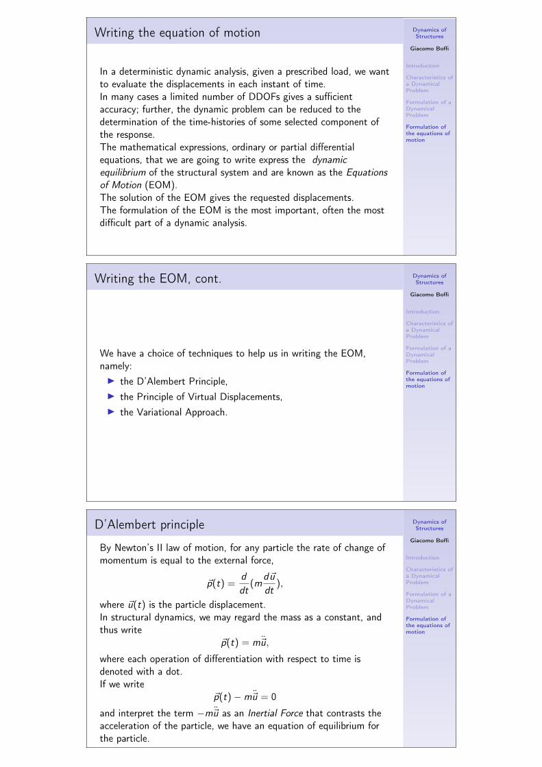
Undamped Free Vibrations
x(t) =exp(iωnt) + exp(−iωnt)
2x0 +
exp(iωnt)− exp(−iωnt)
2ix0ωn
Using the Euler formulas relating the imaginary argumentexponentials and the trigonometric functions, can be rewritten interms of the elementary trigonometric functions
x(t) = x0 cos(ωnt) + (xo/ωn) sin(ωnt).
Considering that for every conceivable initial conditions we can usethe above representation, it is indifferent, and perfectly equivalent,to represent the general integral either in the form of exponentials ofimaginary argument or as a linear combination of sine and cosine ofcircular frequency ωn
Dynamics ofStructures
Giacomo Boffi
1 DOF System
Free vibrations ofa SDOF system
Free vibrations ofa damped system
Undamped Free Vibrations
Otherwise, using the identity exp(±iωnt) = cosωnt ± i sinωnt
x(t) = (A + iB) (cosωnt + i sinωnt) + (C − iD)× (cosωnt − i sinωnt)
expanding the product and evidencing the imaginary part of the responsewe have
I(x) = i (A sinωnt + B cosωnt − C sinωnt − D cosωnt) .
Imposing that I(x) = 0, i.e., that the response is real, we have
(A− C ) sinωnt + (B − D) cosωnt = 0 → C = A, D = B.
Substituting in x(t) eventually we have
x(t) = 2A cos(ωnt)− 2B sin(ωnt).
Dynamics ofStructures
Giacomo Boffi
1 DOF System
Free vibrations ofa SDOF system
Free vibrations ofa damped system
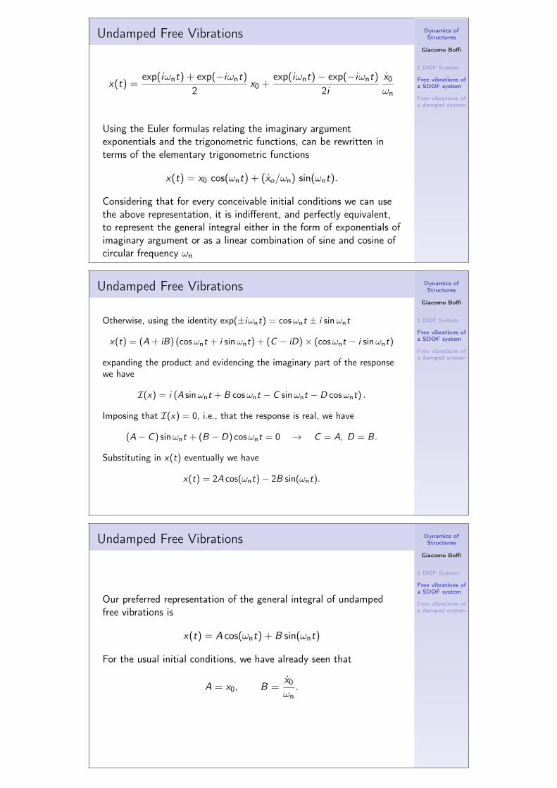
Undamped Free Vibrations
Our preferred representation of the general integral of undampedfree vibrations is
x(t) = A cos(ωnt) + B sin(ωnt)
For the usual initial conditions, we have already seen that
A = x0, B =x0ωn.
Dynamics ofStructures
Giacomo Boffi
1 DOF System
Free vibrations ofa SDOF system
Free vibrations ofa damped system
Undamped Free Vibrations
Sometimes we prefer to write x(t) as a single harmonic, introducinga phase difference φ so that the amplitude of the motion, C , is putin evidence:
x(t) = C cos(ωnt − ϕ) = C (cosωnt cosϕ+ sinωnt sinϕ)
= A cosωnt + B sinωnt
From A = C cosϕ and B = C sinϕ we have tanϕ = B/A, fromA2 + B2 = C 2(cos2 ϕ+ sin2 ϕ) we have C =
√A2 + B2 and
eventually
x(t) = C cos(ωnt − ϕ), with
{C =
√A2 + B2
ϕ = arctan(B/A)
Dynamics ofStructures
Giacomo Boffi
1 DOF System
Free vibrations ofa SDOF system
Free vibrations ofa damped system
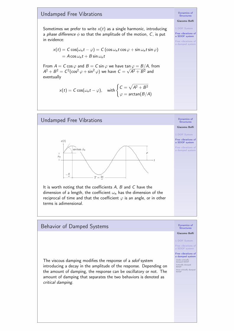
Undamped Free Vibrations
x(t)
t
x0
arctan x0
− θω
T = 2πω
ρ
It is worth noting that the coefficients A, B and C have thedimension of a length, the coefficient ωn has the dimension of thereciprocal of time and that the coefficient ϕ is an angle, or in otherterms is adimensional.
Dynamics ofStructures
Giacomo Boffi
1 DOF System
Free vibrations ofa SDOF system
Free vibrations ofa damped systemUnder-criticallydamped SDOF
Critically dampedSDOF
Over-critically dampedSDOF
Behavior of Damped Systems
The viscous damping modifies the response of a sdof systemintroducing a decay in the amplitude of the response. Depending onthe amount of damping, the response can be oscillatory or not. Theamount of damping that separates the two behaviors is denoted ascritical damping.

Dynamics ofStructures
Giacomo Boffi
1 DOF System
Free vibrations ofa SDOF system
Free vibrations ofa damped systemUnder-criticallydamped SDOF
Critically dampedSDOF
Over-critically dampedSDOF
The solution of the EOM
The equation of motion for a free vibrating damped system is
m x(t) + c x(t) + k x(t) = 0,
substituting the solution exp st in the preceding equation andsimplifying, we have that the parameter s must satisfy the equation
m s2 + c s + k = 0
or, after dividing both members by m,
s2 +c
ms + ω2
n = 0
whose solutions are
s = − c
2m∓√( c
2m
)2− ω2
n = ωn
− c
2mωn∓√(
c
2mωn
)2
− 1
.
Dynamics ofStructures
Giacomo Boffi
1 DOF System
Free vibrations ofa SDOF system
Free vibrations ofa damped systemUnder-criticallydamped SDOF
Critically dampedSDOF
Over-critically dampedSDOF
Critical Damping
The behavior of the solution of the free vibration problem depends of
course on the sign of the radicand ∆ =(
c2mωn
)2− 1:
∆ < 0 the roots s are complex conjugate,∆ = 0 the roots are identical, double root,∆ > 0 the roots are real.
The value of c that make the radicand equal to zero is known as thecritical damping,
ccr = 2mωn = 2√mk .
Dynamics ofStructures
Giacomo Boffi
1 DOF System
Free vibrations ofa SDOF system
Free vibrations ofa damped systemUnder-criticallydamped SDOF
Critically dampedSDOF
Over-critically dampedSDOF
Critical Damping
A single degree of freedom system is denoted as critically damped,under-critically damped or over-critically damped depending on thevalue of the damping coefficient with respect to the critical damping.
Typical building structures are undercritically damped.

Dynamics ofStructures
Giacomo Boffi
1 DOF System
Free vibrations ofa SDOF system
Free vibrations ofa damped systemUnder-criticallydamped SDOF
Critically dampedSDOF
Over-critically dampedSDOF
Damping Ratio
If we introduce the ratio of the damping to the critical damping, orcritical damping ratio ζ,
ζ =c
ccr=
c
2mωn, c = ζccr = 2ζωnm
the equation of free vibrations can be rewritten as
x(t) + 2ζωnx(t) + ω2nx(t) = 0
and the roots s1,2 can be rewritten as
s = −ζωn ∓ ωn√ζ2 − 1.
Dynamics ofStructures
Giacomo Boffi
1 DOF System
Free vibrations ofa SDOF system
Free vibrations ofa damped systemUnder-criticallydamped SDOF
Critically dampedSDOF
Over-critically dampedSDOF
Free Vibrations of Under-critically Damped Systems
We start studying the free vibration response of under-criticallydamped SDOF, as this is the most important case in structuraldynamics.The determinant being negative, the roots s1,2 are
s = −ζωn ∓ ωn√−1√
1− ζ2 = −ζωn ∓ iωD
with the position that
ωD = ωn√
1− ζ2.
is the damped frequency; the general integral of the equation ofmotion is, collecting the terms in exp(−ζωnt)
x(t) = exp(−ζωnt) [G1 exp(−iωDt) + G2 exp(+iωDt)]
Dynamics ofStructures
Giacomo Boffi
1 DOF System
Free vibrations ofa SDOF system
Free vibrations ofa damped systemUnder-criticallydamped SDOF
Critically dampedSDOF
Over-critically dampedSDOF
Initial Conditions
By imposing the initial conditions, u(0) = u0, u(0) = v0, after a bitof algebra we can write the equation of motion for the given initialconditions, namely
x(t) = exp(−ζωnt)
[exp(iωDt) + exp(−iωDt)
2u0+
exp(iωDt)− exp(−iωDt)
2iv0 + ζωn u0
ωD
].
Using the Euler formulas, we finally have the preferred format of thegeneral integral:
x(t) = exp(−ζωnt) [A cos(ωDt) + B sin(ωDt)]
withA = u0, B =
v0 + ζωn u0ωD
.

Dynamics ofStructures
Giacomo Boffi
1 DOF System
Free vibrations ofa SDOF system
Free vibrations ofa damped systemUnder-criticallydamped SDOF
Critically dampedSDOF
Over-critically dampedSDOF
The Damped Free Response
x(t)
t
x0
ρ
T = 2πω
ρ =
√x20 +
(x0+ζωx0
ωD
)2
Dynamics ofStructures
Giacomo Boffi
1 DOF System
Free vibrations ofa SDOF system
Free vibrations ofa damped systemUnder-criticallydamped SDOF
Critically dampedSDOF
Over-critically dampedSDOF
Critically damped SDOF
In this case, ζ = 1 and s1,2 = −ωn, so that the general integral mustbe written in the form
x(t) = exp(−ωnt)(A + Bt).
The solution for given initial condition is
x(t) = exp(−ωnt)(u0 + (v0 + ωn u0)t),
note that, if v0 = 0, the solution asymptotically approaches zerowithout crossing the zero axis.
Dynamics ofStructures
Giacomo Boffi
1 DOF System
Free vibrations ofa SDOF system
Free vibrations ofa damped systemUnder-criticallydamped SDOF
Critically dampedSDOF
Over-critically dampedSDOF
Measuring damping
Over-critically damped SDOF
In this case, ζ > 1 and
s = −ζωn ∓ ωn√ζ2 − 1 = −ζωn ∓ ω
whereω = ωn
√ζ2 − 1
and, after some rearrangement, the general integral for theover-damped SDOF can be written
x(t) = exp(−ζωnt) (A cosh(ωt) + B sinh(ωt))
Note that:I as ζωn > ω, for increasing t the general integral goes to zero,
and thatI as for increasing ζ we have that ω → ζωn, the velocity with
which the response approaches zero slows down for increasing ζ.

Dynamics ofStructures
Giacomo Boffi
1 DOF System
Free vibrations ofa SDOF system
Free vibrations ofa damped systemUnder-criticallydamped SDOF
Critically dampedSDOF
Over-critically dampedSDOF
Measuring damping
Measuring damping
The real dissipative behavior of a structural system is complex andvery difficult to assess.For convenience, it is customary to express the real dissipativebehavior in terms of an equivalent viscous damping.In practice, we measure the response of a SDOF structural systemunder controlled testing conditions and find the value of the viscousdamping (or damping ratio) for which our simplified model bestmatches the measurements.For example, we could require that, under free vibrations, the realstructure and the simplified model exhibit the same decay of thevibration amplitude.
Dynamics ofStructures
Giacomo Boffi
1 DOF System
Free vibrations ofa SDOF system
Free vibrations ofa damped systemUnder-criticallydamped SDOF
Critically dampedSDOF
Over-critically dampedSDOF
Measuring damping
Logarithmic Decrement
Consider a SDOF system in free vibration and two positive peaks, unand un+m, occurring at times tn = n (2π/ωD) andtn+m = (n + m) (2π/ωD).The ratio of these peaks is
unun+m
=exp(−ζωnn2π/ωD)
exp(−ζωn(n + m)2π/ωD)= exp(2mπζωn/ωD)
Substituting ωD = ωn√
1− ζ2 and taking the logarithm of bothmembers we obtain
ln(un
un+m) = δ = 2mπ
ζ√1− ζ2
where we have introduced δ, the logarithmic decrement; solving forζ, we finally get
ζ = δ((2mπ)2 + δ2
)− 12 .
Dynamics ofStructures
Giacomo Boffi
1 DOF System
Free vibrations ofa SDOF system
Free vibrations ofa damped systemUnder-criticallydamped SDOF
Critically dampedSDOF
Over-critically dampedSDOF
Measuring damping
Recursive Formula for ζ
The equation of the logarithmic decrement,
δ = 2mπζ√
1− ζ2
can be formally solved for ζ:
ζ = δ 2mπ√
1− ζ2
obtaining an equation that can be interpreted as generating a sequence
ζn+1 = δ 2mπ√
1− ζ2n .
Starting our sequence of successive approximations with ζ0 = 0 we obtainζ1 = δ 2mπ and usually the following iterate ζ2 = δ 2mπ
√1− ζ21 has converged
to the true value with a number of digits that exceeds the experimental accuracy.
While the recursive formula is useful in itself, it is also useful as a first exampleof finding better approximations of a system’s parameter using an iterativeprocedure.


![Dynamics of Structures - download.e-bookshelf.de · [Dynamique des structures, application aux ouvrages de génie civil. English] Dynamics of structures / Patrick Paultre. p. cm.](https://static.fdocuments.net/doc/165x107/5c8b344f09d3f298038beaaa/dynamics-of-structures-downloade-dynamique-des-structures-application.jpg)


