An Introduction to DynamicalSystems and Chaos

Marc Spiegelman, LDEO

September 22, 1997

This tutorial will develop the basic ingredients necessary for modeling and under-standing simple (and not so simple) non-linear dynamical systems. The goal ofthese exercises are to demonstrate you that you can develop significant insight intothe behavior of complicated non-linear systems with just a little math, a little artand a little modeling software. By themselves, these tools can lead to frustration.However, when combined in the right ways they can give you surprising powersof understanding. The purpose of this tutorial is to give you practice and guidanceinto the basic tricks of the trade so that when you are done you will be able to� Recognize a dynamical system when you see one.� Visualize the behavior of the entire system with just a few tricks� Solve specific instances using STELLA� Understand a systems fixed points and stability� Be happy in phase space� Get a taste of real Chaos

This module contains three labs of increasing complexity that try to highlightthe important concepts of non-linear systems while developing enough basic toolsto be useful. However, these labs are only a brief introduction to a rich and exten-sive subject. For a beautiful but qualitative overview of the subject see Gleick [1].Then read Strogatz [2] for an excellent introduction to the quantitative guts of thebusiness.

Postscript version of Tutorial is here

1

1 Introduction: So what’s a dynamical system any-way?

Dynamics is the study of change, and a Dynamical System is just a recipe for sayinghow a system of variables interacts and changes with time.

�For example, we might

want to understand how an ecology of species interacts and evolves in time so wecan answer questions like, “how robust is this system to small changes” or “if wedecrease the rainfall by 10% or make it erratic, will the system crash and burn?or will some species flourish”. Similar questions can be asked for the economy,the stock market (they may not be the same thing), simplified climate models, orreactive or radioactive chemicals in groundwater. The different systems may seemto be distinct, but they can often be investigated using the same powerful tools.

When we speak of dynamical systems mathematically, we are talking about asystem of equations that describe how each variable (e.g. each species) changeswith time. ��� ���� � � � � ��� �� ������ � ��� � ������� ��� � � � ��� �� ������ � ��� � ���

...�������� � � � � ��� �� ������ � ��� � ���The � species are given by (

� � ����� � ��� ) and the right hand side of each equation is afunction � ��� ����� � � ��� that says how fast that variable changes with time. In general,the rates of change will depend on the values of the other variables and this is whatmakes the business interesting. If they depend on each other in a nonlinear

way,

then things can get really interesting. Nevertheless, the important point is that aslong as we can evaluate the different functions for a given set of variables and time,we can always say something about how the system will evolve. We will use thistrick extensively, to show that you can often understand the behavior of the entiresystems (sometimes) without even solving the differential equations. However, atthis point, things are a bit too abstract so lets start from the very beginning.�

Of course many interesting problems evolve in space as well as time, however, for our purposeshere, we will just consider systems that have no spatial structure (e.g. we will worry about thenumber of animals in a population, but not how they are distributed in space).�

We’ll get to what a non-linear coupling is in a bit

2

2 Lab 1: Simple Systems

The simplest systems have only one variable (hardly a system) but can providesignificant insight into how more complicated things work. In particular they areuseful for demonstrating the basic steps required for creating and understandingquantitative models

1. Formulating the model

2. Analyzing the model

3. Solving the model

4. Understanding the model

5. Accepting (or more likely rejecting) the model

Here we will consider some simple models for population growth of a single species.The first problem is worked out in detail. The second one you’re on your own.

2.1 The Bio-Bomb

Every single species is a potential Bio-Bomb in that if given enough resources thepopulation would simply grow to cover the earth (we’re not doing too badly our-selves). Here we will explore a simple model with this behavior. When we haveunderstood the global behavior of this model we will then ask whether it is actuallya useful model for populations.

2.1.1 Formulation

Most population models are simply a matter of life and death. That is, the growthrate of the number of members of the species depends only on the balance of thebirth rate and the death rate. In our first problem we will make the simple assump-tion that these rates are constant fractions of the current population. For example,consider a population of rabbits. If 25% of the population gives birth to a singleoffspring in a year, the rate of growth due to births would be ������ "! per year where! is the number of rabbits # . Of course, death is important too, and the death ratecould depend on another constant. For example if 5% of the rabbits dies per yearthe death rate would be $%���&�� "! per year. Question: why is the death rate neg-ative?'

more correctly, ( should be the density of rabbits or the average population over some largearea. In this kind of modeling we’ll assume that the population is big enough that ( is not requiredto be an integer

3

More generally, we can assume the that birthrate constant is ) and the deathrate constant is * and therefore the total change in population per year is just*,+*�-/. )0+213*,+ (1)

2.1.2 Model Analysis

The constants ) and * are control parameters of the system and will control thegross structure of the solution. Before we go much further, however, it is worthlooking at the equations and noting that we could make this simpler. By lookingat Equation (1) we can see that the only important thing that affects the popula-tion growth is the difference between the birth and death rate which is 45)617*,89+ .Therefore we we could write the model in a simpler form*,+*�-/.;: + (2)

where :<. 4=)61>*,8 . Now we only have one adjustable parameter, the net growthrate : . In modeling, it is always useful to reduce the number of true parameters totheir smallest number or else you will waste your time solving apparently differentproblems that are actually the same. ?

Now that we have simplified the model, let’s ask the crucial question@ What is the behavior of the entire system for different values of : and differ-ent initial populations +BA ?

At this point, we could jump in to STELLA, slap together a model, and solvefor the population as a function of time and parameters (see Section 2.1.3). To an-swer our question, however, we would need to explore a wide range of values of: and +CA and it would be pretty tedious. Here we will show you that with a bit ofalgebra and a bit of sketching you can analyze the qualitative behavior of the solu-tion without touching the keyboard. To do this we need a graphical representationof exactly what Equation (2) means.

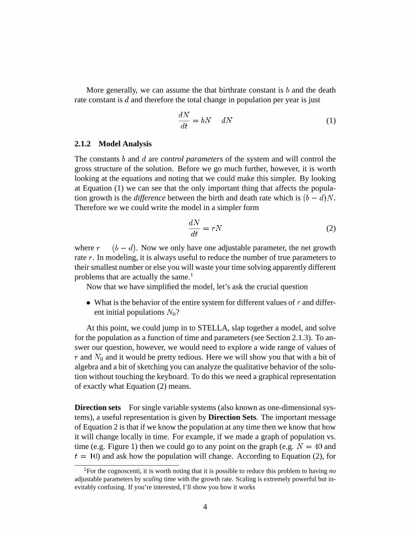
Direction sets For single variable systems (also known as one-dimensional sys-tems), a useful representation is given by Direction Sets. The important messageof Equation 2 is that if we know the population at any time then we know that howit will change locally in time. For example, if we made a graph of population vs.time (e.g. Figure 1) then we could go to any point on the graph (e.g. + . D�E and- . F E

) and ask how the population will change. According to Equation (2), forGFor the cognoscenti, it is worth noting that it is possible to reduce this problem to having no

adjustable parameters by scaling time with the growth rate. Scaling is extremely powerful but in-evitably confusing. If you’re interested, I’ll show you how it works

4

this value of population, the population should increase at a rate of H�IKJ;L bunniesper year. That is, if we took a small step forward in time, we expect that popula-tion would increase. We can plot this change in time and population as an arrowstarting at the point IKJ;M�N and OPJRQSN . The arrow would point to the right and upindicating increasing time and increasing population (this is much easier to do thanto say so I will show it to you). If we started at a higher population (e.g. IKJ;L�N ,the growth rate would be higher and the arrow would increase more steeply for thesame amount of time. This way, we could go to every point in the graph and puta small arrow saying how things would change if we happened to be at that point.The set of arrows is called a direction set and Figure 1 shows some direction setsfor the growth problem for HTJ;N�U�V and HTJRW%N,UXV .

0

20

40

60

80

100

0 5 10 15 20Time (years)

0

20

40

60

80

100

0 5 10 15 20Time (years)

Pop

ulat

ion

(N)Y

Pop

ulat

ion

(N)Y

r=0.2 (growth)Z r=-0.2 (decay)[

Time (years) Time (years)

Figure 1: 1 Direction sets for the simple growth model in equation 2

Inspection of the direction sets gives an immediate feeling for how this problemwill evolve. We can think of the field of arrows as a flow field like currents in a river.In the case of flow in a river, if we dropped a leaf into the flow it would trace outa trajectory in space. In exactly the same way, if we started to solve Equation (2)at any initial population and time, it would also track out a trajectory in the graph,such that at any point, the direction set arrows would be tangent to the trajectory.In general, finding the exact trajectory for a given initial condition can be difficultor impossible analytically, but computer programs like STELLA \ do exactly that.Thus a combination of direction sets for gaining intuition and Stella for solvingspecific instances make for a very powerful combination.]

STELLA is not the only program for solving dynamical systems, it’s just the one we have athand and it has a point and click interface that is not too difficult to play with. If you have accessto X-Windows or Unix, XPP is a very powerful tool for solving dynamical systems. If you preferto do your own programming, MATLAB is a very good environment

5

2.1.3 Solving the problem with STELLA

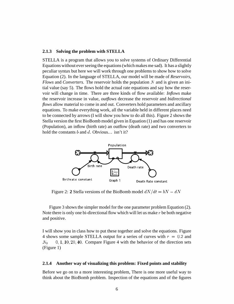
STELLA is a program that allows you to solve systems of Ordinary DifferentialEquations without ever seeing the equations (which makes me sad). It has a slightlypeculiar syntax but here we will work through one problems to show how to solveEquation (2). In the language of STELLA, our model will be made of Reservoirs,Flows and Converters. The reservoir holds the population ^ and is given an ini-tial value (say 5). The flows hold the actual rate equations and say how the reser-voir will change in time. There are three kinds of flow available: Inflows makethe reservoir increase in value, outflows decrease the reservoir and bidirectionalflows allow material to come in and out. Converters hold parameters and ancillaryequations. To make everything work, all the variable held in different places needto be connected by arrows (I will show you how to do all this). Figure 2 shows theStella version the first BioBomb model given in Equation (1) and has one reservoir(Population), an inflow (birth rate) an outflow (death rate) and two converters tohold the constants _ and ` . Obvious... isn’t it?

Figure 2: 2 Stella versions of the BioBomb model `,^bac`�dPe/_0^gfh`�^Figure 3 shows the simpler model for the one parameter problem Equation (2).

Note there is only one bi-directional flow which will let us make i be both negativeand positive.

I will show you in class how to put these together and solve the equations. Figure4 shows some sample STELLA output for a series of curves with ije k�l�m and^Cnoepk�q�r�q�rSk�q�msk�q9t�k . Compare Figure 4 with the behavior of the direction sets(Figure 1)

2.1.4 Another way of visualizing this problem: Fixed points and stability

Before we go on to a more interesting problem, There is one more useful way tothink about the BioBomb problem. Inspection of the equations and of the figures

6

Figure 3: 3 Stella versions of the compact BioBomb model u,vxwsu�yPzj{�v

Figure 4: Example STELLA output for the problem of exponential growth for {Tz|,}X~and initial conditions vB�6z |����"�S�S|���~s|��9��|

shows that for most initial conditions we expect the population to grow or shrinkdepending on the sign of { . However, if we look closer we note that there is a spe-cial initial condition at vC�6z | where nothing happens. I.e. even in a problem withexponential growth, if we start with no rabbits, we’ll alway get no rabbits (This is aspecific case of the important maxim “you can’t get something for nothing”). Thequestion is, whether the fixed point is stable or not, that is if we perturb our startingcondition just a small distance from the fixed point, do we return to the fixed pointor do we fly away. If we return to the fixed point we call it stable, else it’s unstable � .Thus another way to investigate these systems is to first find all the fixed points inthe problem (i.e. values of v where all the equations equal zero), and then inves-tigate their stability. For the simple Bio-bomb problem, it is clear that v�z | is anunstable fixed point if the growth rate is positive but it is stable if the growth rate�

In 1-D systems, it can be proved that the only kind of fixed points are stable and unstable. In2-D things are much more interesting

7

is negative, i.e. for a decay problem, all solutions eventually end up at ����� nomatter where they start. We will consider the behavior of fixed points a bit in thenext problem and considerably in the 2-D problems. For more on fixed points seeStrogatz [2].

2.2 Limits to growth: the logistic equation

Okay, exponential growth and decay is a simple understandable model but is it anygood? It turns out the exponential decay is an excellent model for radioactive wastebut neither decay or growth are particularly good ones for for population. Whynot? One possible answer is that these models don’t allow for anything like a stablepopulation except for the unhappy one of extinction � ��� . In this section youwill redo the analysis for a slightly more useful model of growth called the logisticequation.

2.2.1 Model Formulation

Part of the problem with the simple growth equation (2) is that the rate of growthis constant and doesn’t know anything about the population size. In a real popula-tion, you might expect that as population increases towards some mythical carry-ing capacity the growth rate will slow down as the death rate begins to match thebirth rate. Whether this actually happens is unclear but if it did, one simple way tomodel this would be to modify the growth rate to look something like��� �x��� �S�6����� ���� (3)

where �S� is the rate we would expect for small populations and�

is the carryingcapacity. Question: what happens when ��� � ?

If we do that, then our new model is only a bit more complicated and looks like� ���� � �S�6����� ������ (4)

Note now that the growth rate depends both on the population and the square ofthe population. This is actually a non-linear problem and is much more difficult tosolve analytically. Nevertheless, with the tricks we developed above, it is no harderto understand than the linear exponential growth problem. With that charge...dothe following problems.

2.2.2 Problems

1. Show that this system has two fixed points at �K�/� and ��� � .

8

2. Sketch out the direction sets for the logistic equation for �T�R�X  and ¡¢�¤£S¥�¥and discuss the stability of the two fixed points. Hint: start with a graphwhere ¦ goes from 0–40 and § goes from 0–150.

3. What do you expect to happen if we start with a population that is smallerthan the carrying capacity?

4. How about larger than the carrying capacity?

5. Do you expect any qualitatively different behavior if you change the growthrate � or the carrying capacity ¡ ?

6. Now use Stella to quantitatively solve the logistic equation and test your in-tuition. Produce a plot showing several trajectories for �T�R�X  , ¡¢�R£¨¥"¥ anddifferent starting populations.

7. Do you think that this is a very interesting model? Why or why not?

Extra credit problems Okay, if you liked that then here are a few more thingsto ponder.

1. Non-constant K There is no reason to believe that the carrying capacityneeds to be constant either. If you were pessimistic, you might expect thatthe carrying capacity might decrease with a higher population (pollution,war, disease). Alternatively you could be an optimist and think that the morepeople, the more chances of finding new solutions to increase the carryingcapacity (better technology, medicine whatever).For fun, pick a world thatsuits your personality, then formulate and analyze that model. Then go readJoel Cohen’s book “How many people can the earth support”.

2. Forced systems Another way that the carrying capacity might change is thatit might be forced to change with time for reasons other than the change inpopulations. For example the carrying capacity might change on a seasonalor decadal time scale (you know...summertime...and the living is easy etc.).One simple model is that ¡ oscillates with some amplitude © and periodª

e.g. ¡h«¬¦9­®�¯¡�°c±²£B³/©o´9µ·¶�«¸ s¹º¦9» ª ­¸¼ . This one is quite tricky but try tounderstand the global behavior of the system in the limits of large amplitudeswings and when the period is long or short compared to the growth rate ofthe species. In addition to solutions, it is also interesting to plot the null-clines which are the values of § and

ªwhere the growth-rate is zero. Have

fun and may the force be with you.

9

3 Lab 2: Life on the Phase Plane

In this Lab we will extend our understanding of systems to problems where thereare two interacting variables. Examples include predator-prey problems, two-speciescompetition problems, epidemic models, non-linear oscillators, lasers and love af-fairs! By adding one more degree of freedom we can (sometimes) get a lot morebehavior ½ . Nevertheless, the tools we developed for understanding 1-D systemswill help us a long way in understanding 2-D systems. Most important, by the timewe are done you will understand the importance and beauty of the Phase Plane andnever want to plot anything against time again... . Again, the goal is to developglobal understanding of the behavior of your model and when you are in 2-D themost important trick to remember is to plot your variables against each other.

3.1 Introduction to 2-D systems: Basic concepts

In a 2-D system we will consider dynamical systems that look something like¾�¿¾�À Á Â�Ã�Ä ¿�Å9Æ�Ç (5)¾�ƾ�À Á ÂsÈÉÄ ¿�Å9Æ�Ç (6)

where¿

andÆ

are our two variables of interests.. Examples might include, rab-bits and grass, hosts and parasites or maybe Romeo and Juliet (.. .see Below). Themost important concepts to understand about 2-D systems (and general dynamicalsystems are)Ê the phase planeÊ Flow on the phase planeÊ Phase portraitsÊ Fixed pointsÊ Stability

The Phase plane is a graph where the axes are just our variables¿

andÆ, so

instead of plotting rabbits against time and grass against time, we want to look atthe behavior of rabbits against grass. If we had three variables, the volume thatthey span is known as phase space (beyond three variables, life gets tricky). Flowon the phase plane is exactly the same idea we used in constructing direction setsË

Although we can’t get chaos yet. That takes three variables if their change functions are smoothas we shall see.. .

10

(Figure 1), that is, Equations (6) say that for every point Ì�Í�Î on the phase plane,Ï"Ðand

ÏsÑgive rules for how the point will change in time. If

Ï"Ðis positive Ì will

increase, if negative Ì will decrease. The same is true for Î , so at every point therewill be a little arrow saying where the system will go in a short time step. This iseasier to show than say. Once we know what the flow field looks like, individualsolutions simply trace out trajectories in phase space.

Now in general, where the change functions are not zero, the system will evolvein time along various trajectories. Things get more interesting however, aroundthe few fixed points where things don’t change. At a fixed point both

Ï"Ðand

ÏÉÑare zero so if we start exactly at a fixed point we will never move away from it.The more interesting question is what happens if we start close to a fixed point.Like in the 1-D problem we can have stable attractors and unstable repellers butin two dimensions we can do some other strange things as well. The next problemwill illustrate what can happen. Nevertheless, the basic rule for analysis of a 2-Dsystem is

1. formulate an interesting 2-D problem

2. find the fixed points and categorize their stability

3. sketch out a phase portrait

4. Use stella to solve for a few crucial trajectories

When you are done, you will have a lovely picture that tells you exactly how theentire system will evolve in time. Many times you can guess what will happenwithout even solving the equations. The next example shows how.

3.2 An example: Love Affairs

This problem is shamelessly stolen from Strogatz’s excellent book on non-lineardynamics [2], and originally appeared in his article in Math Magazine [3]. Thisis an example of a linear system because the rate equations depend only on linearcombinations of the variables. Nevertheless it forms an important basis for under-standing non-linear systems. I quote from Strogatz directly

To arouse your interest in the classification of linear systems, we nowdiscuss a simple model for the dynamics of love affairs (Strogatz 1988[3]).The following story illustrates the idea.

Romeo is in love with Juliet, but in our version of this story, Julietis a fickle lover, The more Romeo loves her, the more Juliet wantsto run away and hide. But when Romeo gets discouraged and backsoff, Juliet begins to find him strangely attractive. Romeo, on the other

11

hand tends to echo her: he warms up when she loves him and growscold when she hates him.

Let ÒÔÓ¬Õ�Öp×Romeo’s love/hate for Juliet at time

ÕØ Ó¬Õ�Öp×Juliet’s love/hate for Romeo at time

ÕPositive values of

ÒÚÙ Øsignify love, negative values signify hate. Then

a model for their star-crossed romance isÛ ÒÛ Õ × ØÛ ØÛ Õ × ÜCÒ. . . Ý

Let’s analyze this problem now and then use Stella to test our intuition. I willdo this in class because it’s easier to show than to talk about.

3.3 A menagerie of fixed points

In the previous problem, the fixed point at the origin (

Ò/×;Þ,Ø ×;Þ

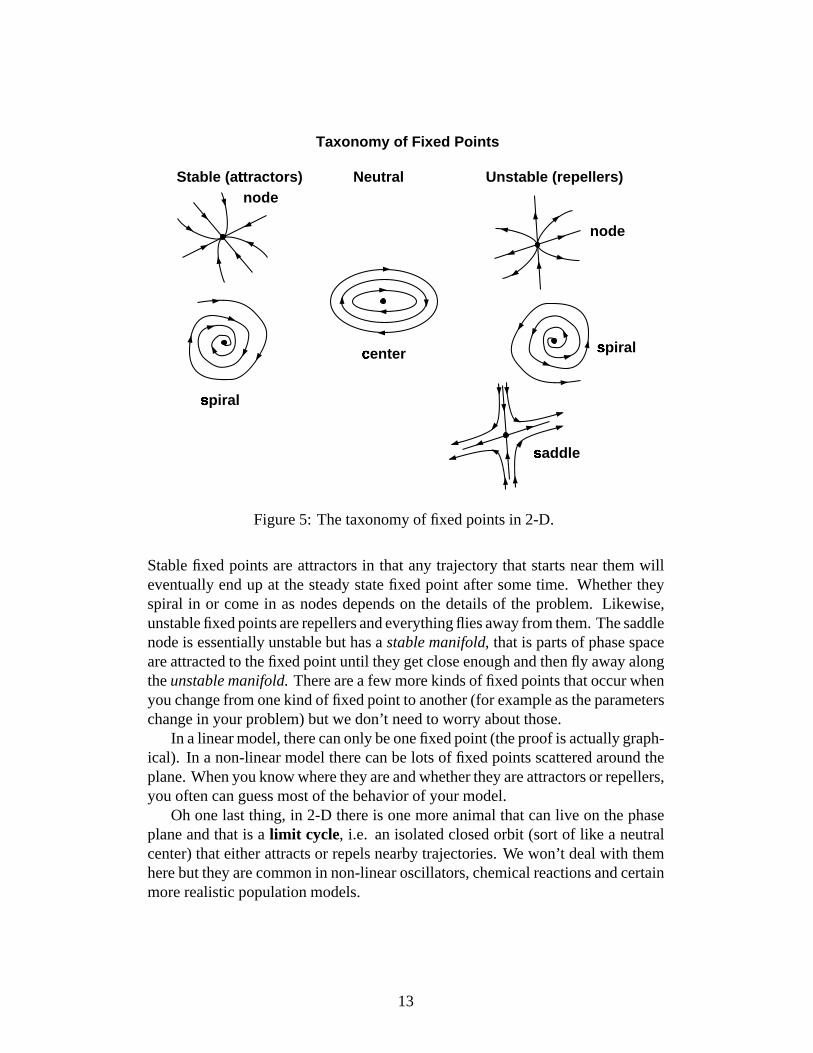
) formed a neu-tral center where trajectories simply orbit around the fixed point. In 2-D there arelots of different ways for system to behave near fixed points. In general, there arefour different qualitative behaviors (plus one more that’s not a fixed point). Theyare ß

Stable nodes and spiralsßUnstable nodes and spiralsßneutral centersßSaddle points

Figure 5 shows them schematically.àIf you’ve peaked ahead, he concludes that.. .”The sad outcome of their affair is, of course,

a never ending cycle of love and hate.. .At least they manage to achieve simultaneous love one-quarter of the time.

12

Taxonomy of Fixed Points

Stable (attractors)á Neutral Unstable (repellers)node

node

spiralâcenterã

saddleâspiralâ

Figure 5: The taxonomy of fixed points in 2-D.

Stable fixed points are attractors in that any trajectory that starts near them willeventually end up at the steady state fixed point after some time. Whether theyspiral in or come in as nodes depends on the details of the problem. Likewise,unstable fixed points are repellers and everything flies away from them. The saddlenode is essentially unstable but has a stable manifold, that is parts of phase spaceare attracted to the fixed point until they get close enough and then fly away alongthe unstable manifold. There are a few more kinds of fixed points that occur whenyou change from one kind of fixed point to another (for example as the parameterschange in your problem) but we don’t need to worry about those.

In a linear model, there can only be one fixed point (the proof is actually graph-ical). In a non-linear model there can be lots of fixed points scattered around theplane. When you know where they are and whether they are attractors or repellers,you often can guess most of the behavior of your model.

Oh one last thing, in 2-D there is one more animal that can live on the phaseplane and that is a limit cycle, i.e. an isolated closed orbit (sort of like a neutralcenter) that either attracts or repels nearby trajectories. We won’t deal with themhere but they are common in non-linear oscillators, chemical reactions and certainmore realistic population models.

13

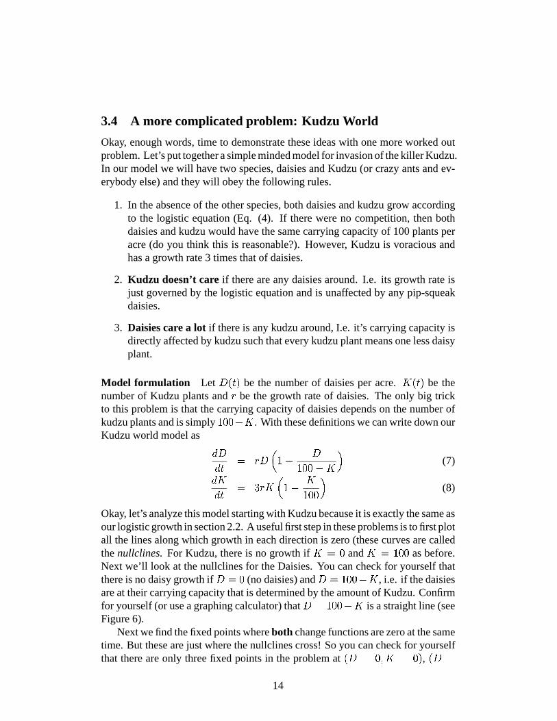
3.4 A more complicated problem: Kudzu World

Okay, enough words, time to demonstrate these ideas with one more worked outproblem. Let’s put together a simple minded model for invasion of the killer Kudzu.In our model we will have two species, daisies and Kudzu (or crazy ants and ev-erybody else) and they will obey the following rules.

1. In the absence of the other species, both daisies and kudzu grow accordingto the logistic equation (Eq. (4). If there were no competition, then bothdaisies and kudzu would have the same carrying capacity of 100 plants peracre (do you think this is reasonable?). However, Kudzu is voracious andhas a growth rate 3 times that of daisies.

2. Kudzu doesn’t care if there are any daisies around. I.e. its growth rate isjust governed by the logistic equation and is unaffected by any pip-squeakdaisies.

3. Daisies care a lot if there is any kudzu around, I.e. it’s carrying capacity isdirectly affected by kudzu such that every kudzu plant means one less daisyplant.

Model formulation Let äxå¬æ9ç be the number of daisies per acre. èhå¬æ�ç be thenumber of Kudzu plants and é be the growth rate of daisies. The only big trickto this problem is that the carrying capacity of daisies depends on the number ofkudzu plants and is simply êSë�ëíì<è . With these definitions we can write down ourKudzu world model as î äî æ ï é�äñð,ê�ì äêSë�ëòì7è�ó (7)î èî æ ï ô é�èõð�ê�ì èêSë�ëöó (8)

Okay, let’s analyze this model starting with Kudzu because it is exactly the same asour logistic growth in section 2.2. A useful first step in these problems is to first plotall the lines along which growth in each direction is zero (these curves are calledthe nullclines. For Kudzu, there is no growth if è ï ë and è ï ê¨ë"ë as before.Next we’ll look at the nullclines for the Daisies. You can check for yourself thatthere is no daisy growth if ä ï ë (no daisies) and ä ï êSë�ëPì÷è , i.e. if the daisiesare at their carrying capacity that is determined by the amount of Kudzu. Confirmfor yourself (or use a graphing calculator) that ä ï ê¨ë"ëøìùè is a straight line (seeFigure 6).

Next we find the fixed points where both change functions are zero at the sametime. But these are just where the nullclines cross! So you can check for yourselfthat there are only three fixed points in the problem at å¸ä ï ë,ú�è ï ë�ç , å¸ä ï

14

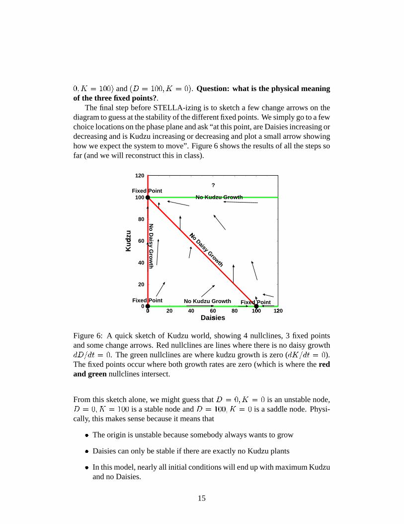
û,ü�ý þ ÿ¨û"û �and ��� þ2ÿSû�û,ü�ý þ û �

. Question: what is the physical meaningof the three fixed points?.

The final step before STELLA-izing is to sketch a few change arrows on thediagram to guess at the stability of the different fixed points. We simply go to a fewchoice locations on the phase plane and ask “at this point, are Daisies increasing ordecreasing and is Kudzu increasing or decreasing and plot a small arrow showinghow we expect the system to move”. Figure 6 shows the results of all the steps sofar (and we will reconstruct this in class).

0� 20 40 60 80 100� 120�Daisies�0

20

40

60

80

100

120

Kud

zu�Fixed Point

Fixed Point Fixed Point

No Kudzu Growth

No Kudzu Growth

No D

aisy Grow

th

No Daisy Growth

?

Figure 6: A quick sketch of Kudzu world, showing 4 nullclines, 3 fixed pointsand some change arrows. Red nullclines are lines where there is no daisy growth ��� � þ û

. The green nullclines are where kudzu growth is zero ( ý � � þ û

).The fixed points occur where both growth rates are zero (which is where the redand green nullclines intersect.

From this sketch alone, we might guess that � þñû,ü�ý þñûis an unstable node,� þ û�ü�ý þ ÿ¨û"û

is a stable node and � þ2ÿSû�û,ü0ý þ ûis a saddle node. Physi-

cally, this makes sense because it means that� The origin is unstable because somebody always wants to grow� Daisies can only be stable if there are exactly no Kudzu plants� In this model, nearly all initial conditions will end up with maximum Kudzuand no Daisies.

15

We can now go into STELLA and make a quantitative phase portrait of the modelto test our understanding. Figure 7 shows that we were right (of course). In par-ticular, this portrait suggests that the entire region of the phase plane for � ���and � ������� is a basin of attraction for Kudzu, i.e. any initial condition thatstarts in this region leads to total Kudzu domination. The problem also poses afew questions to ponder.

1. Do you think that changing the relative growth rates of Daisies and Kudzuaffect their stability? What do the growth rates control?

2. Consider what happens for a trajectory that starts with lots of Daisies andonly one Kudzu plant. At what point should you worry about Kudzu takingover?

3. What happens if you start with a few Daisies and more Kudzu than the car-rying capacity? Whoops! what is wrong with this model?

4. In general, do you think this is a reasonable model for Kudzu invasion? Howwould you test it?

Figure 7: Quantitative phase portrait for the Kudzu invasion problem for a valueof ��� � a carrying capacity of 100, and a set of trajectories starting with just onekudzu plant and a wide range of Daisy populations. Note that all initial conditionsfor ��������� end up with nothing but kudzu.

3.5 Your turn: More problems

Okay, now it’s your turn. There are two problems here plus some extra credit toughies.Get together in groups and choose just one of these problems to explore. If you

16

have the time and inclination, you can do as many as you want...go ahead, knockyour socks off.

3.5.1 A (not so good) predator-prey problem

Here’s another gem from Strogatz. A classic model of predator prey interactionfavored by text-book writers (and dismissed by biologists) is the Lotka-Volterrapredator-prey model which we can think of as rabbits vs. coyotes (or coyotes vs.ACME). If we let �! #"%$ be the number of rabbits and &' #"($ be the number of Coyotesper 100 acres, then we can write this model as) �) " * +�, -/.10 &&32�4 � (9)) &) " * 0 +�5 -6.10 ��72�4 & (10)

where +8, and +�5 are growth rates and &32 and �72 are specific, constant values ofpopulation density of coyotes and rabbits.9 Discuss the biological meaning of each equation and comment on any unre-

alistic assumptions (hint: think of each equation like a simple growth rateequation e.g.

) �;: ) " * + � (Equation 2) but now the growth rate + is afunction of coyotes or rabbits). This is tricky but worth the discussion. Youshould also do it at the end of the problem.9 Show that the two points �� *=</> & *?< $ and ( � * �@2 > & * &32 ) are fixedpoints in this system.9 Extra credit: Prove that those points are the only fixed points (hint: draw thenull-clines).9 Sketch some direction arrows for the phase-plane plot and predict the behav-ior of the two fixed points.9 Choose +8,A* . >(+�5�*�BDC , �72 *EC8< and &32 * . < (or any other values youplease) and use STELLA to test your intuition and show that the model pre-dicts cycles in the populations of both species, for almost all initial condi-tions. (which initial conditions do not produce cycles). What happens if youstart with 1 rabbit and 10 coyotes per 100 acres? Does this make sense toyou? Why or Why not?9 Discuss Strogatz’s point that “This model is popular with many textbookwriters because it’s simple, but some are beguiled into taking it too seriously.Mathematical biologists dismiss the Lotka-Volterra model because it is not

17

structurally stable, and because real predator-prey cycles typically have acharacteristic amplitude. In other words, realistic models should predict asingle closed orbit, or perhaps finitely many, but not a continuous family ofneutrally stable cycles. See the discussions in May (1972) [4], Edelstein-Keshet (1988) [5], or Murray (1989) [6]

3.5.2 More love affairs problem

Here are a bunch of Problems for Romeo and Juliet (kindly appropriated from Stro-gatz). Do the first one and try one more of the last four.

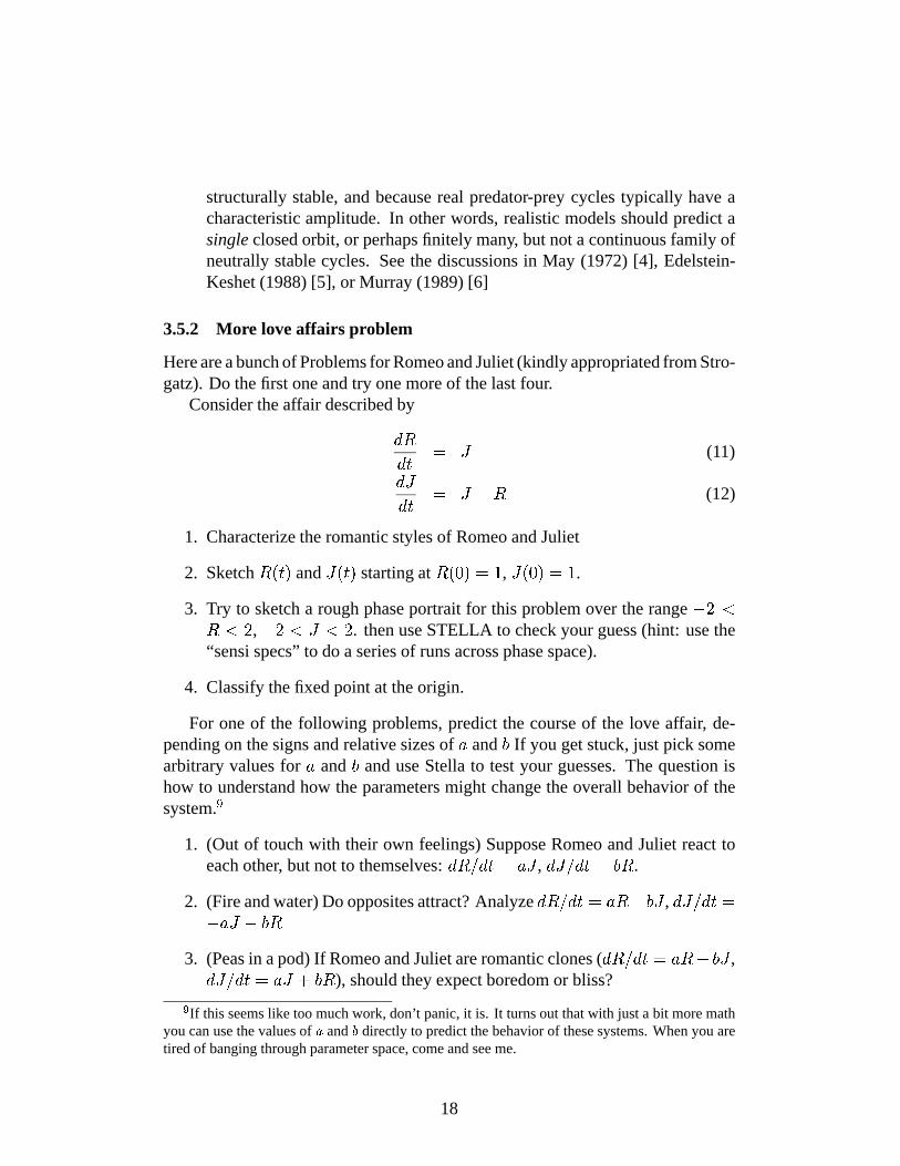
Consider the affair described byF/GF�H I J (11)F JF�H I JLK G (12)

1. Characterize the romantic styles of Romeo and Juliet

2. SketchG!M#H(N

and J M#H(N starting atG!MPOQN I?R , J MSO�N ITR .

3. Try to sketch a rough phase portrait for this problem over the range K;UWVG V=U , K;U�VXJYV=U . then use STELLA to check your guess (hint: use the“sensi specs” to do a series of runs across phase space).

4. Classify the fixed point at the origin.

For one of the following problems, predict the course of the love affair, de-pending on the signs and relative sizes of Z and [ If you get stuck, just pick somearbitrary values for Z and [ and use Stella to test your guesses. The question ishow to understand how the parameters might change the overall behavior of thesystem. \

1. (Out of touch with their own feelings) Suppose Romeo and Juliet react toeach other, but not to themselves:

F/G;]8F�H I Z J ,F J ]^F�H I [ G .

2. (Fire and water) Do opposites attract? AnalyzeF_G`]^F�H I Z Gba [ J ,

F J ]^F�H IK Z JLK [ G3. (Peas in a pod) If Romeo and Juliet are romantic clones (

F_G;]^F�H I Z Gca [ J ,F J ]8F�H I Z J a [ G ), should they expect boredom or bliss?dIf this seems like too much work, don’t panic, it is. It turns out that with just a bit more math

you can use the values of e and f directly to predict the behavior of these systems. When you aretired of banging through parameter space, come and see me.

18

4. (Romeo the robot) Nothing could ever change the way Romeo feels aboutJuliet: g/h;i8g�j'kml , gonpi^g�j'kmq/h�rtsun . Does Juliet end up loving him orhating him?

3.5.3 More fun on the phase plane: Extra credit

1. Do it yourself Shakespeare Make up your own love affair scenario, de-scribe the meaning behind the model and analyze it.

2. A double logistic competition model A much better (and only a bit harder)species competition model than Kudzu world can be writteng/v!wg�j k x8w(v!wzy|{1}~v!w�}�q/v���� (13)g/v��g�j k x���v���y|{1}~v���}~s�v!w(� (14)

where v�w , v�� are populations of species one and two relative to their individ-ual carrying capacity (this is an example of scaling, if v�w�k?{ , it means thatpopulation one is at its carrying capacity in the absence of species 2...tricky,tricky,tricky).The constants q and s affect how much the other species affects each speciesgrowth rate.� Choose q and s to be any numbers less than 1 then sketch a phase por-

trait with nullclines and identify the four fixed points (hint, the graph-ing calculator on the Macs might be useful here). Discuss the stabilityof the different fixed points. Can you get a stable population with bothspecies?� Check your answer with Stella, make a quantitative phase portrait anddiscuss the global behavior of this system for different initial condi-tions.

3. A Parasite-Host problem Okay, enough already... .

4 Lab 3: Onward to Chaos.. .The Lorenz equations

Okay, if we’ve survived through the first two labs we should have a much betterfeel for the concepts of phase-space, fixed points and stability of dynamical sys-tems. However, we still haven’t seen any chaos. As it turns out, I wasn’t beingnice, it just happens to be impossible to get chaos with less than three variables wP� .���

Actually this statement is true as long as the change functions are smooth in a way that canbe made mathematically rigorous (i.e. they have continuous derivatives). When this so, it is im-

19

However, with three variables, things can get very interesting indeed. Herewe will explore one of the classic systems that display chaotic behavior in threevariables: the Lorenz Equations, which were explored (and explained) by EdwardLorenz in his phenomenal 1963 paper [7] ten years before Chaos was “discovered”.Gleick [1] presents this story very nicely. Here we will delve into the quantita-tive aspects of chaos a bit more deeply using the tools we have already developed.When we are done I hope you will have a better understanding of� deterministic chaos� strange attractors� Extreme sensitivity to initial conditions (AKA the butterfly effect)� The predictability of chaotic systems

4.1 Where they come from

The Lorenz equations are not much harder to write down and solve than the sys-tems we have already looked at. The biggest difficulty is actually understandingwhere they come from. To get there, we first have to understand a bit about Ther-mal Convection which is just a fancy name for the idea that hot-air rises and coldair sinks. In physics there is a classic problem ��� of convection in a thin layer offluid that is heated from below (for example a pan with a thin layer of water on astove). This problem can show a remarkable range of behavior depending on howhard you heat the layer. In general, a parcel of fluid that is hotter than its surround-ings will try to do two things. Because it is less dense, it will try to rise like a hot airballoon; however, because it is hot it will also lose heat by cooling. So, if it coolsfaster than it can move it will just sit there. If it has more heat, or loses it moreslowly it will convect. When convection is confined to a thin layer, it can form allkinds of patterns from no flow at all (if you don’t heat it enough) to simple rolls tohighly turbulent chaotic flow (look at a glass tea kettle some time).

Anyway, the Lorenz equations are just a simplified model of thermal convec-tion in a thin sheet. The principal simplification is that Lorenz, pretended that thefluid velocity could be described by a single roll and that the temperature in thelayer could be described by a steady state solution and two time dependent modes.

possible for trajectories to cross because that would imply that the change functions could havedifferent values for the same variables. If something cannot cross in 2-D then the best it can do isloop around on itself���

called Rayleigh Benard Convection

20

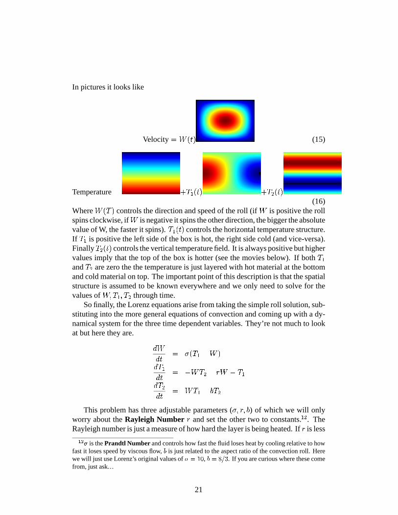
In pictures it looks like

Velocity �����#�%� (15)

Temperature � �@���z�#�%� �7�����#�(�(16)

Where ���#�`� controls the direction and speed of the roll (if � is positive the rollspins clockwise, if � is negative it spins the other direction, the bigger the absolutevalue of W, the faster it spins). �p���#�(� controls the horizontal temperature structure.If �p� is positive the left side of the box is hot, the right side cold (and vice-versa).Finally � ���#�(� controls the vertical temperature field. It is always positive but highervalues imply that the top of the box is hotter (see the movies below). If both �p�and ��� are zero the the temperature is just layered with hot material at the bottomand cold material on top. The important point of this description is that the spatialstructure is assumed to be known everywhere and we only need to solve for thevalues of �W¡¢����¡¢� � through time.

So finally, the Lorenz equations arise from taking the simple roll solution, sub-stituting into the more general equations of convection and coming up with a dy-namical system for the three time dependent variables. They’re not much to lookat but here they are. £ �£ � � ¤��¥����¦~�?�£ �p�£ � � ¦;�§������¨�� ¦Y�p�£ � �£ � � �§���©¦«ª%� �

This problem has three adjustable parameters ( ¤¬¡%¨�¡­ª ) of which we will onlyworry about the Rayleigh Number ¨ and set the other two to constants. �S� . TheRayleigh number is just a measure of how hard the layer is being heated. If ¨ is less®¥¯¢°

is the Prandtl Number and controls how fast the fluid loses heat by cooling relative to howfast it loses speed by viscous flow, ± is just related to the aspect ratio of the convection roll. Herewe will just use Lorenz’s original values of

°`²´³|µ, ± ²·¶z¸­¹ . If you are curious where these come

from, just ask.. .

21

than one, the layer is being heated too gently to convect. Large Rayleigh numbersimply very vigorous convection. The following section will explore the behaviorof the Lorenz equations for different values of the Rayleigh number.

4.2 Behavior of the Lorenz equations

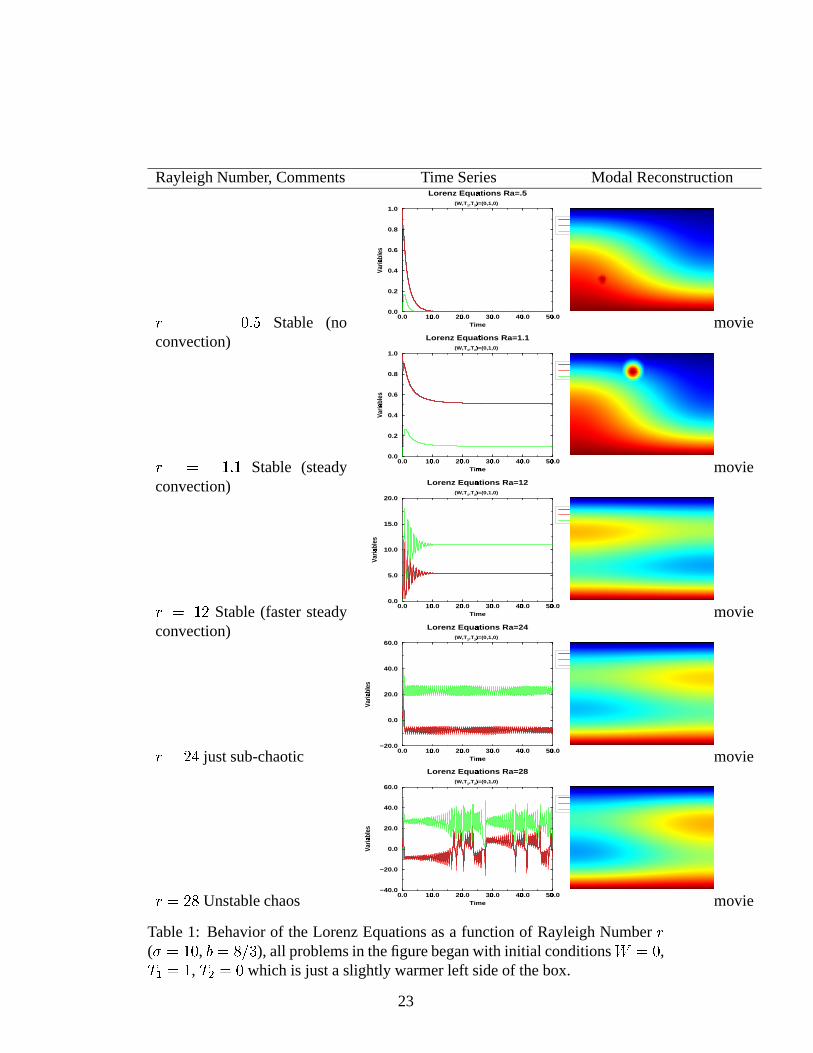
Table 1 shows the behavior of the Lorenz Equations for increasing values of heat-ing. The first figure in each row shows the value of each of the variables º (blackline), »p¼ (red line) and » ½ (green line) as a function of time. The second figureshows a modal reconstruction of the temperature field at time ¾«¿ À (which iswhere the movies begin). At low values of heating Á= à , the initial tempera-ture perturbation cools too fast and the layer stop convecting. For ÁÄ¿?Ã�ÅÆà the rollconvects at a steady velocity clockwise. If we had started the problem with a hotterright hand side ( »�¼ negative), then we would have a roll that rotated the other way.For this problem, as we increase the Rayleigh number to just shy of 25, all initialconditions will eventually settle down to one of two steady states, a roll that eitherrotates clockwise or counter clockwise. As the Rayleigh number is increased, ittakes longer and longer to settle down and the final speed of the roll gets higherand higher. At a critical Rayleigh number (of 24.74 for this problem), however,the roll becomes unstable and we enter the chaotic regime where the roll continu-ously oscillates in time and flips direction in a predictable, yet unpredictable way.Welcome to Chaos

What is surprising about this problem is that these equations are determinis-tic in the sense that for any value of the three parameters, we know exactly howthe behavior will change. Yet if we solve the problem far enough in time, it turnsout that for some cases it is impossible to predict where it will end up. This wasLorenz’s enormous contribution, before these equations it was thought that if youknew enough, the future was predictable. At least in this problem, that is not true.Time to look at these yourself

4.3 Problem 1: Lorenz in phase space

Okay, time for you to play with this beast and start to untangle some of its proper-ties and underlying chaos (and order). Do the following

1. Code up the Lorenz equations in Stella and check their qualitative behavioragainst some of the runs in table 1. Don’t worry if they don’t match wiggle,for wiggle. With these equations, that is impossible. If you have difficultygetting it to work, let me know I have a pre-coded version available. I havefound that most of the behavior can be seen running for about a time of 25with a time step of 0.025. Always use a 4th order Runge Kutta scheme.

22

Rayleigh Number, Comments Time Series Modal Reconstruction

Ç È É/ÊDË Stable (noconvection)

0.0 10.0Ì 20.0Ì 30.0Ì 40.0Ì 50.0ÌTime

0.0

0.2

0.4

0.6

0.8

1.0

Varia

blesÍ

Lorenz Equations Ra=.5Î(W,T1,T2)=(0,1,0)Ï

W(t)TÐ

1(t)TÐ

2(t)

movie

Ç È Ñ�ÊÒÑ Stable (steadyconvection)

0.0 10.0Ì 20.0Ì 30.0Ì 40.0Ì 50.0ÌTimeÓ0.0

0.2

0.4

0.6

0.8

1.0

Varia

blesÍ

Lorenz Equations Ra=1.1Ô(W,T1,T2)=(0,1,0)Ï

W(t)TÐ

1(t)TÐ

2(t)

movie

ÇÕÈ Ñ�Ö Stable (faster steadyconvection)

0.0 10.0Ì 20.0Ì 30.0Ì 40.0Ì 50.0ÌTime

0.0

5.0

10.0

15.0

20.0

Varia

blesÍ

Lorenz Equations Ra=12Î(W,T1,T2)=(0,1,0)Ï

W(t)TÐ

1(t)TÐ

2(t)

movie

Ç�È�Ö^× just sub-chaotic 0.0 10.0Ì 20.0Ì 30.0Ì 40.0Ì 50.0ÌTimeÓ−20.0

0.0

20.0

40.0

60.0

Varia

blesÍ

Lorenz Equations Ra=24Î(W,T1,T2)=(0,1,0)Ï

W(t)ØTÐ

1(t)TÐ

2(t)

movie

Ç�È�Ö8Ù Unstable chaos 0.0 10.0Ì 20.0Ì 30.0Ì 40.0Ì 50.0ÌTime

−40.0

−20.0

0.0

20.0

40.0

60.0

Varia

blesÍ

Lorenz Equations Ra=28Î(W,T1,T2)=(0,1,0)Ï

W(t)TÐ

1(t)TÐ

2(t)

movie

Table 1: Behavior of the Lorenz Equations as a function of Rayleigh Number Ç( Ú È?ÑuÉ , Û È§Ù�Ü8Ý ), all problems in the figure began with initial conditions Þ ÈßÉ ,àpá È?Ñ , à�â ÈßÉ which is just a slightly warmer left side of the box.

23

2. Extra credit: Show by substitution that this problem has 3 fixed points ã�ä åæ_ç¢èpé å æ_ç¢è ê å æ�ë(no motion), ã�ä åíì î�ãPï`ðòñ ë­ç¢è�é åóì î�ãPï`ðôñ ë­ç¢è�ê åãPï;ðõñ ë and ã�ä å�ð ì î�ãPïöðòñ ë�ç¢è�é å�ð ì î�ãPïöðòñ ë�ç¢è�ê å÷ãPï;ðõñ ë two rolls

with different directions.

3. Investigate the evolution of these equations in phase space. Phase space forthis problem is three dimensional but you can see most of the action if youplot ä vs.

è�ê. Do the following

(a) set ï�åTñ æ and make a phase plot comparing two initial conditions withã�ä ç¢èpé�ç¢è�ê�ë å ã æ/ç ñ ç%æQë and ã æ/ç ð�ñ ç%æ�ë . Watch the time series plot atthe same time and try to understand the relationship between the Time-Series and the phase portrait. Try some other initial conditions. Do youthink this solution is stable? What happens when you get near to a fixedpoint?

(b) increase ï to 28 (Lorenz’s famous run) and rerun the the problem from(0,1,0) (this is Lorenz’s famous run, which he did on a Royal McBeeLGP-30 Computing machine at about one second per time step. Sur-prisingly, these Macs aren’t much faster). Plot both the time series forä and the ä ç¢è�ê phase portrait. Now what is the behavior of the fixedpoints (do they attract or repel?) Can you explain qualitatively what ishappening? Can you guess when the solution will flip?

(c) Now explore the “sensitivity to initial conditions”, do 3 runs with ini-tial conditions (0,0.9,0), (0,1,0), (0,1.1,0) (use the sensi spec menu toautomate this). Make a comparison plot for ä vs. time and ä vs.è ê

. How long does it take for the different solutions to go their sep-arate ways? At what point would you consider the behavior chaotic?In phase space, however, note that all the solutions still fall within thefunny butterfly shaped strange attractor. It’s not a fixed point, it’s nota periodic orbit, it’s just strange... .

4.4 Order out of Chaos: The Lorenz equations and prediction

The peculiar result of the Lorenz equations is that they produce deterministic chaos.The problem is deterministic, because we know everything there is about how itwill instantaneously change (there is nothing random about these equations). Forhigh enough Rayleigh numbers, however, it is chaotic because even small changesin the initial conditions can lead to very different behavior at long times becausethe small differences grow in a non-linear feedback with time. This is known asthe Butterfly effect because Lorenz suggested that a butterfly flapping in one partof the world might make it impossible to predict the weather a week in advance.

24

Nevertheless, Chaos does not mean random unpredictability. After watchingthese equations flip and flop for a while, you can see that in some respects they arefairly well behaved. The overall behavior is restricted to lie in the Strange attractor(the system can’t suddenly stop or start spinning a thousand times faster) and theoverall patterns repeat in a quasi-periodic fashion. The problem is that you can’tfollow the problem for an arbitrarily long period of time.

But watching these equations perform, you might get the feeling that you shouldbe able to follow them for some period of time. If you consider each wobble in theproblem a cycle, then Lorenz actually showed that you can actually predict the be-havior of the equations at least one cycle ahead. Here we will reproduce that result(and more) and introduce some of the basics of non-linear forecasting.

Here is the basic problem. Suppose that you were handed a time-series of ø ù(or anything else, maybe rainfall in Arizona). You might want to ask yourself “howmuch information is in this time-series...if I know a part of it, how much into thefuture can I predict?” This is the basic question of non-linear forecasting (e.g. [8,9]). If you’re data is produced by a low dimensional chaotic attractor, the answermay be that you can predict more than you thought.

What Lorenz asked was “if I know the peak value of ø ù at some time, can Ipredict the value of the next peak?” To do this he first formed a series of all themaximum values of ø�ù with time (i.e. he had a list of peak1,peak2,.. . ,peakN), thenfor each peak ú he made a plot of peak ú6ûYü as a function of peak ú (easier to showthan say). And he found the following remarkable picture known as The LorenzMap

What is remarkable about this picture, is how narrow the graph is. While it is nota line, it is so narrow, that except maybe very near the peak, you have an excellentchance of predicting the size of the next peak if you know the size of the currentone. Order out of Chaos indeed. ýPþ What I want to do now though is find out if it ispossible to repeat this feat for 2 cycles in the future, 3 cycles etc. I.e. the questionis how far can you predict into the future?

To answer that, do the following problems

1. Reproduce the Lorenz Map. I’ve already made a file with a large number ofpeak values in it (the run was made at very high precision for ÿ�� ���

for atime of 100). Get a copy of the file T2max.txt and load it into Excel. Thenform a second column that is a repeat of the first, except that it starts with thesecond value (this is easier to do than it sounds, I’ll show you). Plot columnA against column B and voila! the Lorenz Map.

���You might be wondering how it is possible to have something that is this well behaved for one

cycle and poorly behaved for many. That’s a slightly different story to do with discrete maps andI will tell it if I have time.

25

30 40 50 60Height of Peak N

30

40

50

60

Hei

ght o

f Pea

k N

+1

30 40 50 60Height of Peak N

30

40

50

60

Hei

ght o

f Pea

k N

The Lorenz Map�r=32, σ=10, b=8.3

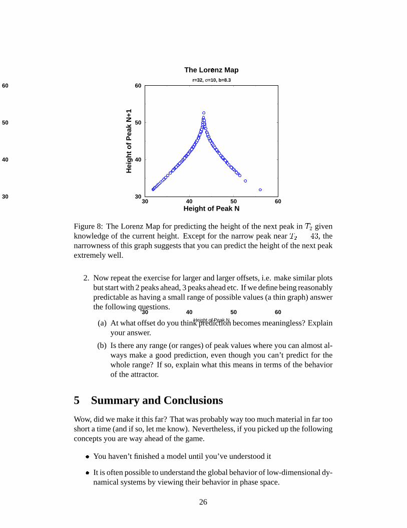
Figure 8: The Lorenz Map for predicting the height of the next peak in � givenknowledge of the current height. Except for the narrow peak near �� ���� , thenarrowness of this graph suggests that you can predict the height of the next peakextremely well.

2. Now repeat the exercise for larger and larger offsets, i.e. make similar plotsbut start with 2 peaks ahead, 3 peaks ahead etc. If we define being reasonablypredictable as having a small range of possible values (a thin graph) answerthe following questions.

(a) At what offset do you think prediction becomes meaningless? Explainyour answer.

(b) Is there any range (or ranges) of peak values where you can almost al-ways make a good prediction, even though you can’t predict for thewhole range? If so, explain what this means in terms of the behaviorof the attractor.

5 Summary and Conclusions

Wow, did we make it this far? That was probably way too much material in far tooshort a time (and if so, let me know). Nevertheless, if you picked up the followingconcepts you are way ahead of the game.

� You haven’t finished a model until you’ve understood it

� It is often possible to understand the global behavior of low-dimensional dy-namical systems by viewing their behavior in phase space.

26

� By mapping out the fixed points and attractors, we can get an intuitive un-derstanding of how small changes in our system will effect the outcome.

� Low dimensional chaos is still understandable and predictable. The impor-tant measure is how much can your predict.

� In some non-linear systems small changes can change the stability of thewhole system. We need to understand how resilient, our much more com-plicated system is to various kinds of forcing.

References

1 J. Gleick. Chaos, Penguin, 1987, Q172.5.C45G54.

2 S. H. Strogatz. Nonlinear Dynamics and Chaos: with applications to physics,biology, chemistry, and engineering, Addison-Wesley Publishing Co., Reading,MA, 1994.

3 S. H. Strogatz. Love affairs and differential equations, Math Magazine 61, 35,1988.

4 R. M. May. Limit cycles in predator-prey communities, Science 177, 900, 1972.

5 L. Edelstein-Keshet. Mathematical Models in Biology, Random House, NewYork, 1988.

6 J. Murray. Mathematical Biology, Springer, New York, 1989.

7 E. N. Lorenz. Deterministic non-periodic flow, J. Atmos. Sci. 20, 130, 1963.

8 G. Sugihara and R. M. May. Nonlinear forecasting as a way of distinguishingchaos from measurement error in time series, Nature 344, 734–, Apr 1990.

9 G. Sugihara. Nonlinear forecasting for the classification of time series, Phil.Trans. R. Soc. London A 348, 477–495, Sep 1994.

27