An Introduction to Control Theory Applications with...
152
An Introduction to Control Theory Applications with Matlab Lazaros Moysis Michail Tsiaousis Nikolaos Charalampidis Maria Eliadou Ioannis Kafetzis August 31, 2015
Transcript of An Introduction to Control Theory Applications with...
An Introduction to Control Theory Applications withMatlab
Lazaros Moysis Michail Tsiaousis Nikolaos CharalampidisMaria Eliadou Ioannis Kafetzis
August 31, 2015

An Introduction to Control Theory Applications with MatlabLazaros Moysis ([email protected])Michail Tsiaousis (mixalis [email protected])Maria Eliadou (maria [email protected])Ioannis Kafetzis ([email protected])Nikolaos Charalampidis ([email protected])
Editing and coordination: Lazaros Moysis http://users.auth.gr/lazarosm/
MATLAB®, Simulink® and Control Systems Toolbox™ are trademarks of the Math-Works, Inc. The MathWorks does not warrant the accuracy of the text or exercises inthis book. This books use or discussion of MATLAB®, Simulink® and Control SystemsToolbox™ software or related products does not constitute endorsement or sponsorship bythe MathWorks of a particular pedagogical approach or particular use of the MATLAB®,Simulink® and Control Systems Toolbox™ software.
Copyright © 2015 Lazaros Moysis, Michail Tsiaousis, Nikolaos Charalampidis, MariaEliadou, Ioannis Kafetzis
This work is licensed under the Creative Commons Attribution-NonCommercial-ShareAlike4.0 International License. To view a copy of this license, visit http://creativecommons.org/licenses/by-nc-sa/4.0/.

Contents
0 Preface 6
1 Basic Matlab Commands 71.1 Introduction . . . . . . . . . . . . . . . . . . . . . . . . . . . . . . . . . . . 71.2 Input Data . . . . . . . . . . . . . . . . . . . . . . . . . . . . . . . . . . . 81.3 Math Operations and Functions . . . . . . . . . . . . . . . . . . . . . . . . 91.4 Graphs and Figures . . . . . . . . . . . . . . . . . . . . . . . . . . . . . . . 101.5 Examples . . . . . . . . . . . . . . . . . . . . . . . . . . . . . . . . . . . . 13
2 Transfer Function Models 172.1 Introduction . . . . . . . . . . . . . . . . . . . . . . . . . . . . . . . . . . . 172.2 Basic polynomial functions . . . . . . . . . . . . . . . . . . . . . . . . . . . 17
2.2.1 Examples . . . . . . . . . . . . . . . . . . . . . . . . . . . . . . . . 182.3 Analysis of a rational function to partial fractions . . . . . . . . . . . . . . 19
2.3.1 Examples . . . . . . . . . . . . . . . . . . . . . . . . . . . . . . . . 192.4 Transfer function . . . . . . . . . . . . . . . . . . . . . . . . . . . . . . . . 20
2.4.1 Examples . . . . . . . . . . . . . . . . . . . . . . . . . . . . . . . . 22
3 System Characteristics and Responses 253.1 System Characteristics . . . . . . . . . . . . . . . . . . . . . . . . . . . . . 253.2 Responses . . . . . . . . . . . . . . . . . . . . . . . . . . . . . . . . . . . . 263.3 Examples . . . . . . . . . . . . . . . . . . . . . . . . . . . . . . . . . . . . 30
4 Dynamic Behavior of First-Order and Second-Order Systems 394.1 First-Order and Second-Order System’s Features . . . . . . . . . . . . . . . 394.2 Examples . . . . . . . . . . . . . . . . . . . . . . . . . . . . . . . . . . . . 41
5 Systems with Delay 475.1 Introduction . . . . . . . . . . . . . . . . . . . . . . . . . . . . . . . . . . . 475.2 Defining a Delay System in Matlab . . . . . . . . . . . . . . . . . . . . . . 47
5.2.1 Defining a Delay system by its transfer function . . . . . . . . . . . 475.2.2 Pade Approximation . . . . . . . . . . . . . . . . . . . . . . . . . . 485.2.3 Delay Systems in Simulink . . . . . . . . . . . . . . . . . . . . . . . 49
3
CONTENTS 4
5.2.4 Example . . . . . . . . . . . . . . . . . . . . . . . . . . . . . . . . . 50
6 System Interconnections 526.1 Subsystem Connection Types . . . . . . . . . . . . . . . . . . . . . . . . . 526.2 Simulink . . . . . . . . . . . . . . . . . . . . . . . . . . . . . . . . . . . . . 556.3 Examples . . . . . . . . . . . . . . . . . . . . . . . . . . . . . . . . . . . . 60
7 State Space Systems 627.1 Introduction . . . . . . . . . . . . . . . . . . . . . . . . . . . . . . . . . . . 627.2 State space representation . . . . . . . . . . . . . . . . . . . . . . . . . . . 62
7.2.1 Examples . . . . . . . . . . . . . . . . . . . . . . . . . . . . . . . . 64
8 Pole Placement 698.1 Introduction . . . . . . . . . . . . . . . . . . . . . . . . . . . . . . . . . . . 698.2 Basic definitions and functions . . . . . . . . . . . . . . . . . . . . . . . . . 698.3 Pole placement through state feedback . . . . . . . . . . . . . . . . . . . . 718.4 Examples . . . . . . . . . . . . . . . . . . . . . . . . . . . . . . . . . . . . 72
9 Observer Design 779.1 Introduction . . . . . . . . . . . . . . . . . . . . . . . . . . . . . . . . . . . 779.2 Observer Construction Example . . . . . . . . . . . . . . . . . . . . . . . . 78
10 Root Locus Analysis 8210.1 Introduction . . . . . . . . . . . . . . . . . . . . . . . . . . . . . . . . . . . 8210.2 Root Locus method . . . . . . . . . . . . . . . . . . . . . . . . . . . . . . . 8210.3 Examples . . . . . . . . . . . . . . . . . . . . . . . . . . . . . . . . . . . . 87
11 Nyquist Plot 9211.1 Introduction . . . . . . . . . . . . . . . . . . . . . . . . . . . . . . . . . . . 9211.2 Nyquist Criterion . . . . . . . . . . . . . . . . . . . . . . . . . . . . . . . . 9211.3 Examples . . . . . . . . . . . . . . . . . . . . . . . . . . . . . . . . . . . . 97
12 Control Systems Toolbox 10612.1 Introduction . . . . . . . . . . . . . . . . . . . . . . . . . . . . . . . . . . . 10612.2 Designing the system . . . . . . . . . . . . . . . . . . . . . . . . . . . . . . 10612.3 Examples . . . . . . . . . . . . . . . . . . . . . . . . . . . . . . . . . . . . 111
13 Designing Controllers Using the Control Systems Toolbox 11613.1 Introduction . . . . . . . . . . . . . . . . . . . . . . . . . . . . . . . . . . . 11613.2 Improving Transient Response . . . . . . . . . . . . . . . . . . . . . . . . . 116
13.2.1 Examples . . . . . . . . . . . . . . . . . . . . . . . . . . . . . . . . 11713.3 Improving Steady State Response . . . . . . . . . . . . . . . . . . . . . . . 126
13.3.1 Examples . . . . . . . . . . . . . . . . . . . . . . . . . . . . . . . . 127

CONTENTS 5
14 Discrete Time Systems 12914.1 Introduction . . . . . . . . . . . . . . . . . . . . . . . . . . . . . . . . . . . 12914.2 Discretization . . . . . . . . . . . . . . . . . . . . . . . . . . . . . . . . . . 12914.3 Examples . . . . . . . . . . . . . . . . . . . . . . . . . . . . . . . . . . . . 132
15 Nonlinear Systems 13815.1 Introduction . . . . . . . . . . . . . . . . . . . . . . . . . . . . . . . . . . . 13815.2 Examples . . . . . . . . . . . . . . . . . . . . . . . . . . . . . . . . . . . . 138
Acknowledgments 146
Bibliography 147
Chapter 0
Preface
During the academic year of 2015, a series of seminars were presented on the MathematicsDepartment of Aristotle University of Thessaloniki, titled “An introduction to Matlabwith Control Theory Applications”. These seminars were conducted by PhD studentL. Moysis and were part of the undergraduate courses ”Classic Control Theory” (7thsemester) and ”Modern Control Theory” (8th semester), both taught by Prof. N. P.Karampetakis.
The aim of these seminars was to present the programming environment of Matlab,Simulink and the Control Systems Toolbox and cover all the important functions andpossibilities that one has to know in order to design and solve a control problem. Thesyllabus of the seminars was based on [Nise, 2013] and [Ogata, 2009], both of which con-stitute excellent books on the theory of control systems.
Upon completion of these courses, we decided to gather all the subjects covered intothis short, yet thorough book.
This book can serve as a companion manual to all undergraduate and postgraduatestudents who are taking a course in Control Theory and want to see examples of systems,implemented and solved in Matlab. Problems from Classic and Modern Control Theoryare covered, like analysis of 1st and 2nd order systems, root locus techniques, controllerdesign, pole placement, observer design and more. These subjects are engaged throughnumerous physical applications which we believe the readers will find intriguing.
We hope that the present textbook will be useful to anyone trying to grasp the conceptof Control Theory. Since this is the collective work of various people (undergraduate andpostgraduate students as well as PhD students) we wish to apologise in advance for anyinconsistencies encountered throughout the text. For any suggestions or corrections, feelfree to contact us at [email protected].
The writing team
6
Chapter 1
Basic Matlab Commands
1.1 Introduction
Matlab is one of the most powerful tools in computation, numerical analysis and systemdesign. Its user friendly environment, in addition to its powerful computational kerneland graphical visualization capabilities make it an integral part of the control systemdesign, optimization and implementation.
Along with the basic Matlab command package, several additional toolboxes have beendeveloped for specific purposes that extend Matlab’s capabilities. Examples are Simulink,Control Systems Toolbox, Fuzzy Logic Toolbox, Image Processing Toolbox, Statistics andMachine Learning Toolbox and many more.
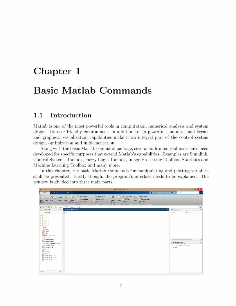
In this chapter, the basic Matlab commands for manipulating and plotting variablesshall be presented. Firstly though, the program’s interface needs to be explained. Thewindow is divided into three main parts.
7

CHAPTER 1. BASIC MATLAB COMMANDS 8
The Command Window is the main window where the commands are inputed. TheCurrent Directory shows the directory from which Matlab runs the files and functions wehave created. Command History shows the history of all the commands that we inputinto the Command Window. The main menu has three different tabs, HOME, PLOTSand APPS. From the Home tab the appearance and layout of Matlab can be changed.
1.2 Input Data
Matlab’s basic data structure is the matrix. Of course scalar variables and vector belongto the same category of data. In order to define a new variable in matlab, the followingformula is used
variable name= value% orvariable name= value;
where value represents a numerical value. The ; at the end of the command determineswhether the result will be displayed on screen or not. For example, if we define a 1000column array representing a time interval, there is no point in displaying the result onscreen. From the above code it is also seen that we use the symbol % to input commentsin our code.
There are two more useful methods of inputting data. The first one is the formula tobe used when creating matrices, which is
M=[a,b; c,d]
where the symbols [] represent the beginning and end of a matrix and the symbol ; here isused to denote a new line of the matrix. Needles to say, when defining a matrix variablethe number of elements in each row must be the same, otherwise an error message isdisplayed. To choose among certain elements of a matrix, one can simply use parentheses() to define which element or which parts of the matrix are to be chosen. To do so, insidethe parentheses the specific rows and columns are specified. To choose all the columns orall the rows, use the symbol :. This will be made clear in the next example.
The second formula is useful when creating arrays of equally spaced numbers. This isparticularly useful when creating time intervals, but is also used inside ”for” loops. Thecommand is
t=a:step:b
where a and b represent numbers and step is the step value used. If the step is omitted,the default value is 1. A second way uses the following command
CHAPTER 1. BASIC MATLAB COMMANDS 9
t=linspace(a, b, n)
that creates an array of n equally spaced numbers between a and b. As an example, thefollowing commands
M=[1 5 10, 6 7 8]t1=0:2:5t2=linspace(0,5,4)M(1,2)M(:,2)M(1,[2 3])
create three variables with the following values
M =
(1 5 106 7 8
)t1 = 0 2 4 t2 = 0 1.6667 3.3333 5.0000
and the last 2 commands create the arrays
5
(57
) (5 10
)One last useful command is the clear command, which deletes any variable in the
workspace. Its syntax is the following
clear variable name % deletes variableclear %deletes all variablesclc % clears the command window (does not delete any variables)
1.3 Math Operations and Functions
There are many already available functions that the users can use in order to solve aproblem. The typical syntax for a function is to call the function using the desired inputarguments. The function will return its outputs, which should be saved in new variablesi.e.
[output1,output2,. . .]=function name(input1,input2,. . .)
the simplest examples of matlab functions are cos(x), sin(x), tan(x), log(x), ...
exp(x), sqrt(x) that take as an input a numerical variable and return a unique output.An example of a more complex Matlab function is ss(a,b,c,d) that is used to definea new state space system and requires four input arguments. It should be noted here

CHAPTER 1. BASIC MATLAB COMMANDS 10
that for calling a multi-input multi-output function, one uses parentheses for the inputarguments and brackets for the multiple variable assignments.
In general, in order to find out about a function’s syntax, input and output argumentsand general informations about its functionality, the command
help function name
displays all the available information on the function, as well as examples and otherrelevant functions. Try for example help eig.
Regarding mathematical operations, Matlab uses the traditional symbols + - * ...
ˆ /. What should be noted though, is that Matlab treats the operators using linearalgebra rules. So if one wishes to use element-wise operations, this should be specifiedusing .* .ˆ ./ instead. For example, in order to obtain the square of each element in avector, the following commands should be used
t=0:0.1:10; % Example of a vectort.ˆ2 % In order to obtain the square of each element% The command tˆ2 tries to multiply t*t, which is wrong since it does ...
not satisfy the linear algebra rules.
Some other useful matrix functions are the following
inv(M) Matrix inversepinv(M) Pseudoinverseeig(M) Eigenvalues of a matrixeye(r,c) Create an r × c matrix with ones in the diagonalzeros(r,c) Zero r × c matrixrand(r,c) An r×c matrix of pseudo random values drawn from the
standard uniform distribution on the open interval(0,1)diag(M) Diagonal matrix with the elements M in its diagonalm' Conjugate transpose of matrix m
1.4 Graphs and Figures
Plotting is one of the most useful applications of any programming language. Matlaboffers a variety of plotting tools that help visualize data, both continuous and discrete.
In order to plot a function, three basic steps are required. First define the range ofvalues over which we wish to plot the function, then define the function and lastly, call aplotting command.
Depending on the kind of data we wish to visualize, different plot commands shouldbe used. The most basic are covered in the following table
CHAPTER 1. BASIC MATLAB COMMANDS 11
plot(x,y,'details') Plots vector y versus vector x. In 'details', graphdetails are entered (optional)
plot3(x,y,z) Plots a line in R3 through the points whose coordinatesare (x,y,z)
surf(x,y,z) Plots the coloured parametric surface defined by (x,y,z)surfc(x,y,z) Plots the coloured parametric surface defined by (x,y,z)
in combination with a contour plotmesh(x,y,z) Plots the coloured parametric mesh defined by (x,y,z)meshc(x,y,z) Plots the coloured parametric mesh defined by (x,y,z) in
combination with a contour plotcontour(x,y,z) Contour plot, i.e. the level curves of function z over the
coordinates (x,y)
in the plot command, the optional argument 'details' is a string containing informa-tion about the way the data are plotted. The string can contain one character from eachof the following columns
b blue . point - solidg green o circle : dottedr red x x-mark -. dashdotc cyan + plus -- dashedm magenta * star (none) no liney yellow s squarek black d diamondw white v triangle (down)
ˆ triangle (up)< triangle (left)> triangle (right)p pentagramh hexagram
For example, the commands
t=0:0.2:2*pi;x=cos(t);plot(t,x,'--')
will plot the cosine signal over [0,2π] and plot its graph as a dashed line, as will be seenin the following examples.
Other useful commands to change the appearance of a figure are the following

CHAPTER 1. BASIC MATLAB COMMANDS 12
xlabel('text') Text on the x-axisylabel('text') Text on the y-axistitle('text') Title textgrid Puts grid on the graphaxis on Displays the axesaxis off Hides the axesaxis square Makes the figure squareaxis equal Makes the unit of measure equal to both axesaxis([ xmin xmax ymin ymax]) Sets axes limitshold on Holds the current plotlegend('first', 'second',. . .) Inserts legend
Now, what happens if the user desired to plot different functions on the same figure, whilekeeping the previous ones too. That is useful for example when we want to observe thechanges in the response of the system under perturbations of a single parameter. Bydefault, the plot command will plot a new figure in the same window, deleting the oldones. In order to keep the previous plots, one can use the command hold all. Forexample, using
t=0:0.2:2*pi;x=cos(t);y=5*cos(t);plot(t,x)hold allplot(t,y)
will draw these 2 functions on the same graph, using different colours for them.On the other hand, what if we want to plot new data on different windows? Matlab
offers two options for this. We can either create a new blank figure with a different keynumber, or create a subplot.
In the first option, simply by inputting the command figure(n) Matlab creates anew blank figure under the key number n = 1, 2, .... all plot commands following thiscommand will be visualised in this new window.
On the other hand, the command subplot(n,m,i) creates a figure and splits it inn rows and m columns. Every new plot command will be visualised in the subfigure atposition i, counting from right to left and top to bottom. To move to another subfigure jwe enter the command subplot(n,m,j). So for example:
t=0:0.2:2*pi;x=cos(t);y=sin(t);subplot(1,2,1)plot(t,x)subplot(1,2,2)
CHAPTER 1. BASIC MATLAB COMMANDS 13
plot(t,y)
will plot a 2× 2 figure having the cosine graph on the first window and the sine graph onthe second window. Examples of these commands are given in the next section.
1.5 Examples
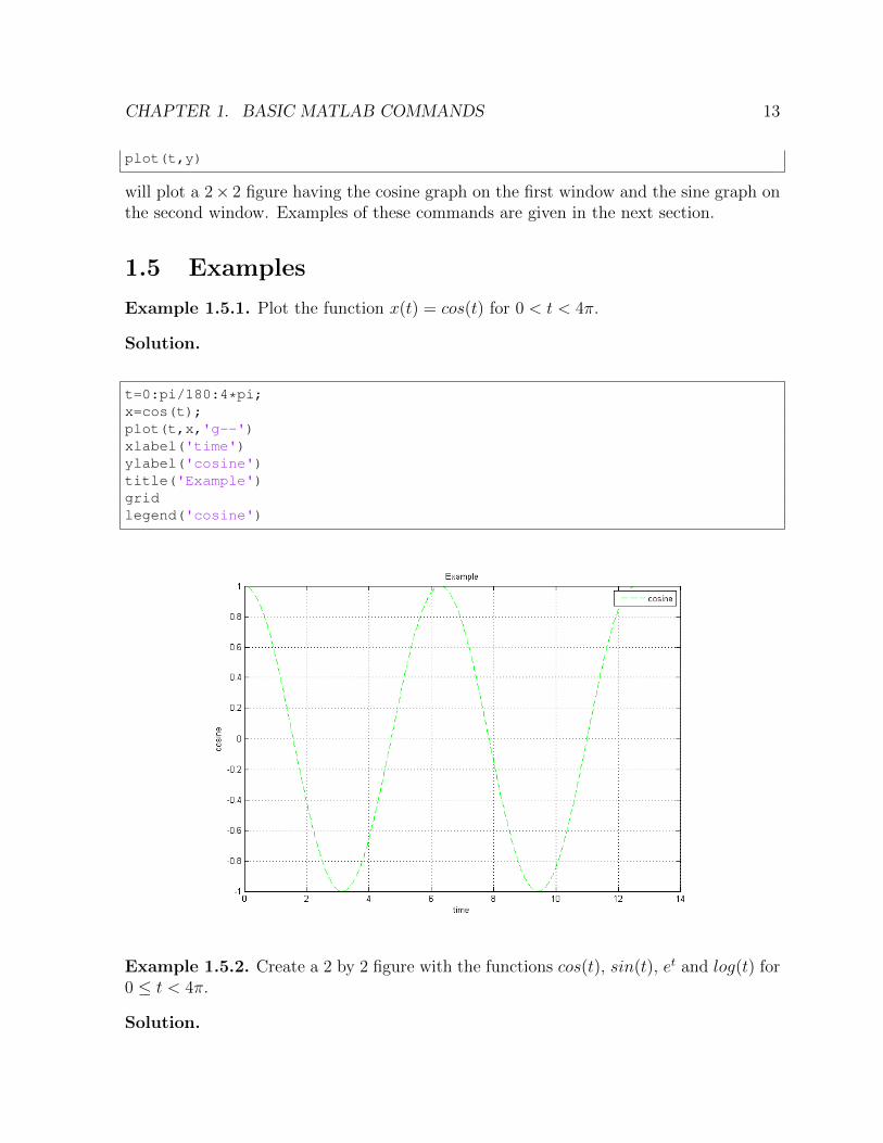
Example 1.5.1. Plot the function x(t) = cos(t) for 0 < t < 4π.
Solution.
t=0:pi/180:4*pi;x=cos(t);plot(t,x,'g--')xlabel('time')ylabel('cosine')title('Example')gridlegend('cosine')
Example 1.5.2. Create a 2 by 2 figure with the functions cos(t), sin(t), et and log(t) for0 ≤ t < 4π.
Solution.

CHAPTER 1. BASIC MATLAB COMMANDS 14
t=0:0.1:4*pi;subplot(2,2,1)plot(t,cos(t))title('cosine')gridsubplot(2,2,2)plot(t,sin(t))title('sine')gridsubplot(2,2,3)plot(t,exp(t))title('exponential')gridsubplot(2,2,4)plot(t,log(t))title('log')grid
Example 1.5.3. Plot the function x(t) = eλt for λ = −1,−2,−3,−4 and 0 ≤ t < 10 onthe same graph.
Solution.
t=0:0.1:10;hold allfor i=1:4
plot(t,exp(-i*t))endgrid
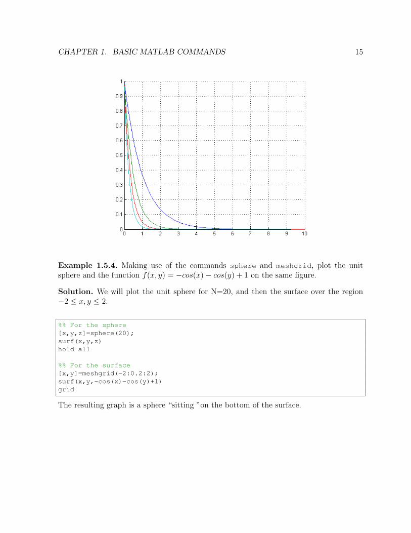
CHAPTER 1. BASIC MATLAB COMMANDS 15
Example 1.5.4. Making use of the commands sphere and meshgrid, plot the unitsphere and the function f(x, y) = −cos(x)− cos(y) + 1 on the same figure.
Solution. We will plot the unit sphere for N=20, and then the surface over the region−2 ≤ x, y ≤ 2.
%% For the sphere[x,y,z]=sphere(20);surf(x,y,z)hold all
%% For the surface[x,y]=meshgrid(-2:0.2:2);surf(x,y,-cos(x)-cos(y)+1)grid
The resulting graph is a sphere “sitting ”on the bottom of the surface.
CHAPTER 1. BASIC MATLAB COMMANDS 16
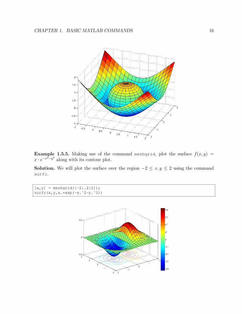
Example 1.5.5. Making use of the command meshgrid, plot the surface f(x, y) =x · e−x2−y2 along with its contour plot.
Solution. We will plot the surface over the region −2 ≤ x, y ≤ 2 using the commandsurfc.
[x,y] = meshgrid([-2:.2:2]);surfc(x,y,x.*exp(-x.ˆ2-y.ˆ2))

Chapter 2
Transfer Function Models
2.1 Introduction
In this chapter, we introduce the concept of the transfer function. We will present differentways of creating a transfer function both in polynomial and factored form and show howto convert from one form to the other. To do so, we first present and give examples ofbasic polynomial functions, since the use of polynomials is required in defining transferfunctions.
2.2 Basic polynomial functions
We define polynomials in Matlab using row vectors. Specifically, in order to define apolynomial we create a row vector where the elements of the latter are the coefficients ofthe polynomial we want to insert.Generally, if we have the polynomial p(t) = ant
n + an−1tn−1 + · · ·+ a1t+ a0 we can define
it in Matlab by typing p=[an . . . a1 a0] in the command window.In order to find the polynomial value for a specific value of the variable, we use the
command
p value = polyval(p,k)
One can also calculate the roots of a polynomial, using
r = roots(p)
where p is the polynomial.It is possible to convert from a symbolic polynomial to a polynomial matrix and vice
versa. We can achieve this with the commands
17

CHAPTER 2. TRANSFER FUNCTION MODELS 18
sym2poly(sym)
and
poly2sym(vector)
respectively. The variable sym denotes the symbolic polynomial we use, to convert to apolynomial vector and the variable vector denotes the vector polynomial we use, to convertto a symbolic polynomial. A similar command to sym2poly(sym) is the command
coeff = coeffs(sym)
Returns the coefficients of the polynomial sym with respect to all variables. The differencebetween these two commands is that coeffs(sym) returns non-zero coefficients startingfrom the lowest order variable.
2.2.1 Examples
Example 2.2.1. Consider the polynomial p(t) = t2 − 2t+ 1
1. Define the polynomial.
2. Calculate the polynomial’s roots.
3. Calculate the value of the polynomial for t = 1.
Solution.
p = [1 -2 1]; % We insert the polynomial as a row vectorr = roots(p)p value = polyval(p,1)
Example 2.2.2. Consider the symbolic polynomial p(t) = t3 + 2t+ 6.
1. Convert the symbolic polynomial to polynomial matrix.
2. Convert the polynomial matrix back to the symbolic polynomial.
Solution.
syms tsym = tˆ3+2*t+6;poly = sym2poly(sym) % Convert symbolic polynomial to polynomial matrixsym again = poly2sym(poly) % Convert back to symbolic polynomial

CHAPTER 2. TRANSFER FUNCTION MODELS 19
Example 2.2.3. Consider the polynomial p(t) = 8t6 + 4t5 − 2t3 + 7t+ 2.Extract the coefficients of this polynomial.
Solution.
syms tp = 8*tˆ6+4*tˆ5-2*tˆ3+7*t+2;coeff = coeffs(p) % Extract coefficients to an array
2.3 Analysis of a rational function to partial fractions
Analysing a rational function to partial fractions is important due to the fact that, wehave the ability to represent the function (transfer function) in a different way, such ashaving the poles of the system as the denominators of the partial fractions. There arealso practical reasons, such as making it easier to find the inverse laplace transform of atransfer function. A partial fraction expansion of a rational function is the following
b(s)
a(s)=
c1
s− p1
+c2
s− p2
+ · · ·+ cns− pn
+ ks
where pi, i = 1, . . . , n the poles of the system, ci, i = 1, . . . , n the residues and ks thequotient We analyse a rational function to partial fractions by using the command
[c,p,k] = residue(num,den)
Matlab then returns residues ci, poles pi, i = 1, 2, . . . , n and direct quotient ks in column-wise order. Variable k (ks), is usually constant or zero. In case k equals zero, Matlab willreturn [ ]. On the other hand, command
[num,den] = residue(c,p,k)
returns the numerator and denominator of the rational function that corresponds in thisparticular analysis.
2.3.1 Examples
Example 2.3.1. Consider the rational function
X(s) =s+ 2
s3 + 4s2 + 3s
Analyse the rational function X(s) as partial fractions.
Solution.

CHAPTER 2. TRANSFER FUNCTION MODELS 20
num=[1 2];den=[1 4 3 0];[c,p,k]=residue(num,den)
We derive that
X(s) =s+ 2
s3 + 4s2 + 3s= −0.1667
s+ 3− 0.5
s+ 1+
0.6667
s
Example 2.3.2. Find the rational function X(s) that corresponds to the following sumof partial fractions
3
s− 1+
1.5
s+ 4.3+−1
s− 2+ 2
Solution.
c = [3;1.5;-1];p = [1;-4.3;2];k = 2;[num,den] = residue(c,p,k)
From the above results, we conclude that
3
s− 1+
1.5
s+ 4.3+−1
s− 2+ 2 =
2s3 + 6.1s2 − 22.7s− 1.3
s3 + 1.3s2 − 10.9s+ 8.6= X(s)
2.4 Transfer function
A transfer function is a rational function of a complex variable that represents a lineartime invariant dynamical system with zero initial conditions. It describes the relationbetween the input and the output of the system. Given r(t) to be the input signal withLaplace transform R(s) and c(t) the output signal with Laplace transform C(S), the ratioof the output C(S) to the input R(s) is
C(s)
R(s)= G(s) =
bmsm + bm−1s
m−1 + · · ·+ b0
ansn + an−1sn−1 + · · ·+ a0
We call this ratio G(s) a transfer function. The above equation separates the input R(s),output C(s) and the system G(s), a feature that we are not able to achieve with differentialequations. We can represent the transfer function as a block diagram

CHAPTER 2. TRANSFER FUNCTION MODELS 21
In order to create a transfer function, one can use the command
sys = tf(num,den)
It creates a continuous-time transfer function with numerator and denominator specifiedby num and den.
Another way of creating a transfer function is by using the zero-pole-gain model, inorder to create a transfer function in factored form. The advantage of this model incomparison to the previous one, is that it gives us a straight-forward way of finding thezeros and the poles of our system. A zero-pole-gain model has the following form:
H(s) = K(s− z1)(s− z2) . . . (s− zn)
(s− p1)(s− p2) . . . (s− pn)
where zi, i = 1, . . . , n are the zeros of our system, pi, i = 1, . . . , n are the poles of oursystem and K is the gain. For a zero-pole-gain model we use
sys = zpk(z,p,k)
where variable z and p are arrays, containing the zeros and the poles of our systemrespectively and variable k is the gain, which is a constant. In case we don’t have zerosin our transfer function, just input z = [ ].
Additionally, we can convert from one model to the other, i.e from polynomial formto factored form and the opposite, using the same commands. Consider that variablesys contains the transfer function created by tf(num,den). In order to convert to azero-pole-gain model, we can use
sys zpk = zpk(sys)
We can also use the following commands
[z,p,k] = tf2zp(num,den);sys = zpk(z,p,k)
Command tf2zp(num,den) takes as input the numerator and the denominator of thetransfer function and returns variables z,p,k containing the zeros, poles and the gainrespectively. Then, we simply take the factored form with the command zpk(z,p,k).
On the other hand, let variable sys contain a transfer function created by zpk(z,p,k).In order to convert to the tf model (polynomial form) we can use
sys tf = tf(sys)

CHAPTER 2. TRANSFER FUNCTION MODELS 22
Alternatively we can use,
[num,den] = zp2tf(z,p,k);sys = tf(num,den)
Command zp2tf(z,p,k) does the exact opposite to tf2zp(num,den). This time, in-puts are the zeros, poles and the gain and the result is the numerator and the denominatorof the transfer function.
Finally, a third way of creating a transfer function, is by assigning a variable, forexample 's', as a variable of the transfer function. Then, simply type the transferfunction in the command window. This is a more convenient way, in case we handlesubsystems, every one of them with its own transfer function, and the transfer functionof the final system is still unknown. In such a case, one can use
s = tf('s');% ors = zpk('s')
in order to assign variable s as a variable of the transfer function.We can still convert from polynomial form to factored form and the opposite. By
using
s = tf('s');
and then writing the transfer function in factored form, Matlab will return the transferfunction in polynomial form. On the other hand, by using
s = zpk('s');
and then writing the transfer function in polynomial form, Matlab will return the transferfunction in factored form.
2.4.1 Examples
Example 2.4.1. Create the following transfer function using tf(num,den)
H(s) =s+ 1
s2 + 3s+ 1
and then convert from tf model (polynomial form) to zpk model (factored form).
Solution.
CHAPTER 2. TRANSFER FUNCTION MODELS 23
num = [1 1];den = [1 3 1];sys = tf(num,den) % Create transfer functionsys zpk = zpk(sys) % Convert to zpk model
Example 2.4.2. Create the following transfer function using zpk(z,p,k)
G(s) =s+ 2
(s+ 1)2(s+ 3)
and then convert from zpk model to tf model.
Solution.
z = -2;p = [-1 -1 -3];k = 1;sys = zpk(z,p,k) % Create zpk modelsys tf = tf(sys) % Convert to tf model
Example 2.4.3. Create the following transfer function by assigning a variable, as avariable of the transfer function.
K(s) =s+ 1
s2 + 2s+ 1
Then, convert this transfer function from polynomial form to factored form.
Solution.
s = tf('s'); % Assign variable s, as variable of the transfer functionsys = (s+1)/(sˆ2+2*s+1)
s = zpk('s');sys = (s+1)/(sˆ2+2*s+1) % Returns transfer function in factored form
Example 2.4.4. Create the following transfer function by assigning a variable, as avariable of the transfer function
T (s) =(s+ 2)(s− 1)
(s+ 3)2(s− 5)
Then, convert this transfer function from factored form to polynomial form.
Solution.

CHAPTER 2. TRANSFER FUNCTION MODELS 24
s = zpk('s'); % Assign variable s, as variable of the transfer functionsys = ((s+2)*(s-1))/((s+3)ˆ2*(s-5))
s = tf('s');sys = ((s+2)*(s-1))/((s+3)ˆ2*(s-5)) % Returns transfer function in ...
polynomial form
Chapter 3
System Characteristics andResponses
In this chapter methods for calculating the response of a system to different inputs (step,impulse, arbitrary) are presented. In addition, the different characteristics of the transient(rise time, overshoot, settling time) and steady state response (steady state error) of firstand second order systems are presented.
3.1 System Characteristics
Some of the most basic characteristics that play an important role in system analysis areof course the poles and the zeros of a system. In order to obtain these, one can use thefollowing commands:
pole(sys) Poles of the transfer functionzero(sys) Zeros of the transfer function[w,z,p]=damp(sys) Returns the natural frequency and damping factor of
each pole in the vector ppzmap(sys) Pole-Zero map of the transfer function
The last two commands are especially interesting, since the damp command can giveuseful information for the frequency and damping factor of the system poles. The pzmapalthough interesting, is usually not used, since rlocus has much more interesting features.
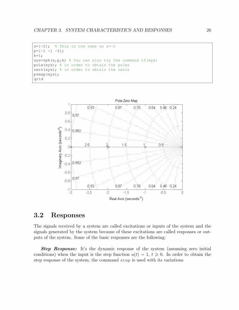
Example 3.1.1. Find the poles and zeros of the following transfer function and plotthem in the Complex plane.
H(s) =s+ 2
(s+ 1)2(s+ 3)
Solution.
25
CHAPTER 3. SYSTEM CHARACTERISTICS AND RESPONSES 26
z=[-2]; % This is the same as z=-2p=[-1 -1 -3];k=1;sys=zpk(z,p,k) % You can also try the command tf(sys)pole(sys); % in order to obtain the poleszero(sys); % in order to obtain the zerospzmap(sys);grid
3.2 Responses
The signals received by a system are called excitations or inputs of the system and thesignals generated by the system because of these excitations are called responses or out-puts of the system. Some of the basic responses are the following:
Step Response: It’s the dynamic response of the system (assuming zero initialconditions) when the input is the step function u(t) = 1, t > 0. In order to obtain thestep response of the system, the command step is used with its variations

CHAPTER 3. SYSTEM CHARACTERISTICS AND RESPONSES 27
step(sys) Plots the step response of the system sysstep(sys, Tfinal) Plots the step response from t = 0 to the final time
t = Tfinalstep(sys, t) uses the user-supplied time vector t for simulationdata=stepinfo('sys') Computes the step response characteristicsv=step(sys) Saves the response in a vector
Example 3.2.1. Consider a system with transfer function:
G(s) =s+ 2
s2 + 4s+ 3
Find the step response of the system.
Solution.
sys=tf([1 2],[1 4 3]);step(sys)
Impulse Response: It’s the dynamic response of the system when our input is theimpulse function δ(t). In order to obtain the step response of the system, the commandstep is used with its variations

CHAPTER 3. SYSTEM CHARACTERISTICS AND RESPONSES 28
impulse(sys) Plots the impulse response of the system sysimpulse(sys, Tfinal) Plots the impulse response from t = 0 to the final time
t = Tfinalimpulse(sys, t) uses the user-supplied time vector t for simulation
Example 3.2.2. Consider the following transfer function:
G(s) =s+ 2
s2 + 4s+ 3
Find the impulse response of the system.
Solution.
sys=tf([1 2],[1 4 3]);impulse(sys)
Arbitrary Response: We can compute the response of a system to any desiredsignal, by creating our own input. In order to do so, we first need to specify the time vectort and the input vector u. After these vectors are defined, the command lsim(sys,u,t)
along with its variations, simulates the response of the system to the given input.
CHAPTER 3. SYSTEM CHARACTERISTICS AND RESPONSES 29
lsim(sys,u,t) Response of the system to input ulsim(sys,u,t,x0) Response of the system to input u with initial conditions
x0
v=lsim(sys,u,t) Saves the response in a vector
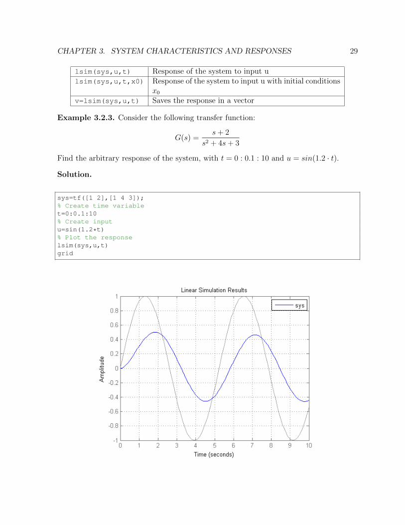
Example 3.2.3. Consider the following transfer function:
G(s) =s+ 2
s2 + 4s+ 3
Find the arbitrary response of the system, with t = 0 : 0.1 : 10 and u = sin(1.2 · t).
Solution.
sys=tf([1 2],[1 4 3]);% Create time variablet=0:0.1:10% Create inputu=sin(1.2*t)% Plot the responselsim(sys,u,t)grid
CHAPTER 3. SYSTEM CHARACTERISTICS AND RESPONSES 30
3.3 Examples
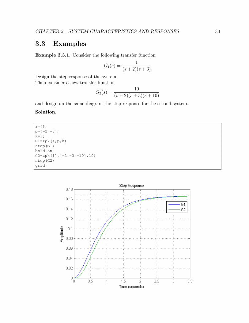
Example 3.3.1. Consider the following transfer function
G1(s) =1
(s+ 2)(s+ 3)
Design the step response of the system.Then consider a new transfer function
G2(s) =10
(s+ 2)(s+ 3)(s+ 10)
and design on the same diagram the step response for the second system.
Solution.
z=[];p=[-2 -3];k=1;G1=zpk(z,p,k)step(G1)hold onG2=zpk([],[-2 -3 -10],10)step(G2)grid

CHAPTER 3. SYSTEM CHARACTERISTICS AND RESPONSES 31
Example 3.3.2. Consider a system with transfer function
H(s) = −2s
(s+ 2)(s2 + 2s+ 2)=
−2s
s3 + 4s2 + 6s+ 4
Define the transfer function to Matlab. Then in a tab with two sub-windows design theimpulse and step response of the system.
Solution.
Hsys=tf([-2 0],[1 4 6 4])subplot(1,2,1)step(Hsys,10)gridsubplot(1,2,2)impulse(Hsys,10)grid
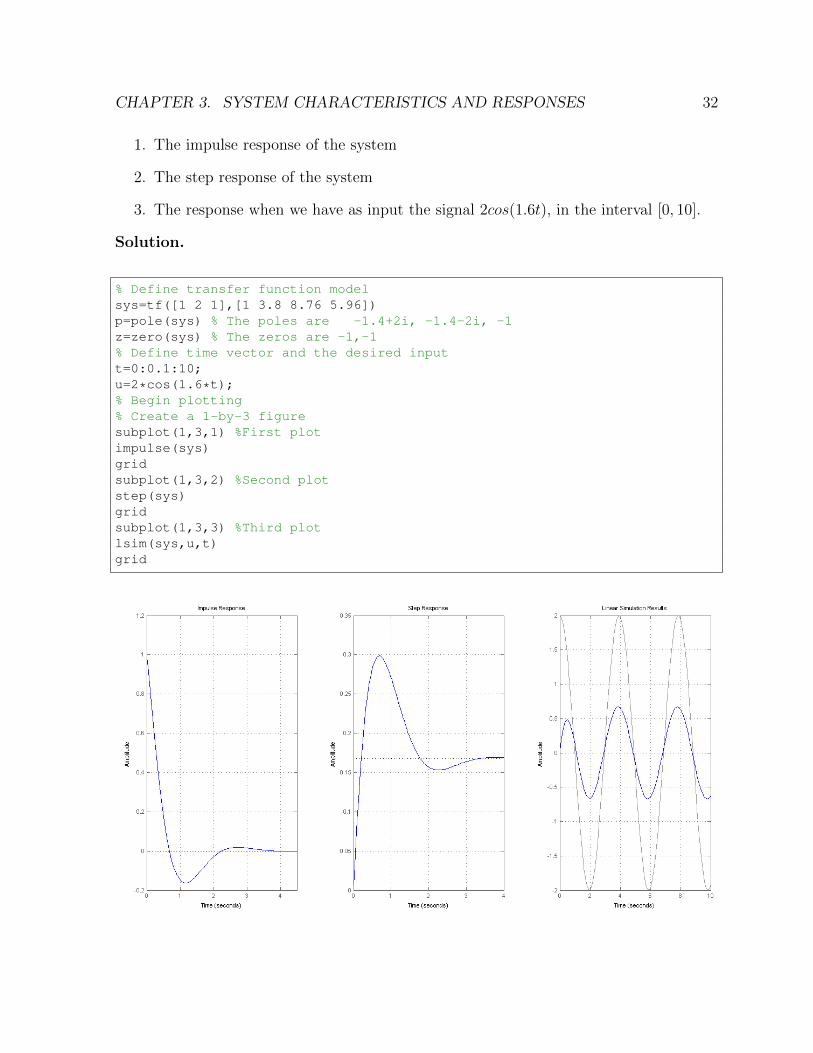
Example 3.3.3. Consider a system with the following transfer function:
G(s) =s2 + 2s+ 1
s3 + 3.8s2 + 8.76s+ 5.96
Find the poles and zeros of the system and then in a tab with 3 sub-windows plot:
CHAPTER 3. SYSTEM CHARACTERISTICS AND RESPONSES 32
1. The impulse response of the system
2. The step response of the system
3. The response when we have as input the signal 2cos(1.6t), in the interval [0, 10].
Solution.
% Define transfer function modelsys=tf([1 2 1],[1 3.8 8.76 5.96])p=pole(sys) % The poles are -1.4+2i, -1.4-2i, -1z=zero(sys) % The zeros are -1,-1% Define time vector and the desired inputt=0:0.1:10;u=2*cos(1.6*t);% Begin plotting% Create a 1-by-3 figuresubplot(1,3,1) %First plotimpulse(sys)gridsubplot(1,3,2) %Second plotstep(sys)gridsubplot(1,3,3) %Third plotlsim(sys,u,t)grid

CHAPTER 3. SYSTEM CHARACTERISTICS AND RESPONSES 33
Example 3.3.4. [Nise, 2013, Stefani, 1973] During an experiment, a human sitting infront of a switch reacts to an optical signal by lowering the switch. The transfer functionwhich connects the human response P (s) (output) to the optical stimulus V (s) is
G(s) =P (s)
V (s)=
s+ 0.5
(s+ 2)(s+ 5)(3.1)
What is the step response of the above system and after find the system’s features(overshoot, rise time, peak time, settling time)
Solution.
z=-0.5;p=[-2 -5];k=1;sys=zpk(z,p,k)step(sys)grid
CHAPTER 3. SYSTEM CHARACTERISTICS AND RESPONSES 34
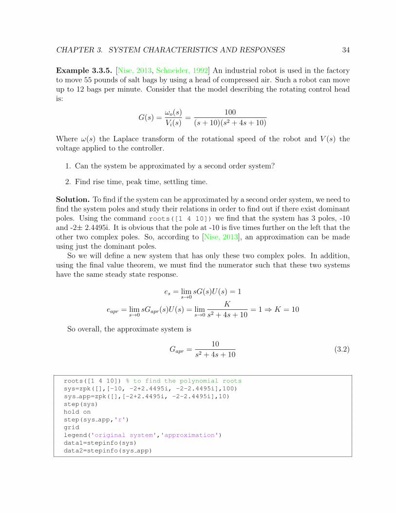
Example 3.3.5. [Nise, 2013, Schneider, 1992] An industrial robot is used in the factoryto move 55 pounds of salt bags by using a head of compressed air. Such a robot can moveup to 12 bags per minute. Consider that the model describing the rotating control headis:
G(s) =ωo(s)
Vi(s)=
100
(s+ 10)(s2 + 4s+ 10)
Where ω(s) the Laplace transform of the rotational speed of the robot and V (s) thevoltage applied to the controller.
1. Can the system be approximated by a second order system?
2. Find rise time, peak time, settling time.
Solution. To find if the system can be approximated by a second order system, we need tofind the system poles and study their relations in order to find out if there exist dominantpoles. Using the command roots([1 4 10]) we find that the system has 3 poles, -10and -2± 2.4495i. It is obvious that the pole at -10 is five times further on the left that theother two complex poles. So, according to [Nise, 2013], an approximation can be madeusing just the dominant poles.
So we will define a new system that has only these two complex poles. In addition,using the final value theorem, we must find the numerator such that these two systemshave the same steady state response.
es = lims→0
sG(s)U(s) = 1
eapr = lims→0
sGapr(s)U(s) = lims→0
K
s2 + 4s+ 10= 1⇒ K = 10
So overall, the approximate system is
Gapr =10
s2 + 4s+ 10(3.2)
roots([1 4 10]) % to find the polynomial rootssys=zpk([],[-10, -2+2.4495i, -2-2.4495i],100)sys app=zpk([],[-2+2.4495i, -2-2.4495i],10)step(sys)hold onstep(sys app,'r')gridlegend('original system','approximation')data1=stepinfo(sys)data2=stepinfo(sys app)
CHAPTER 3. SYSTEM CHARACTERISTICS AND RESPONSES 35
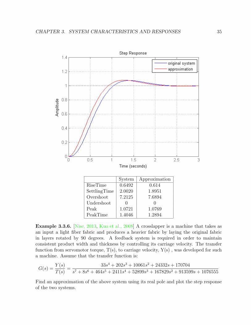
System ApproximationRiseTime 0.6492 0.614SettlingTime 2.0020 1.8951Overshoot 7.2125 7.6894Undershoot 0 0Peak 1.0721 1.0769PeakTime 1.4046 1.2894
Example 3.3.6. [Nise, 2013, Kuo et al., 2008] A crosslapper is a machine that takes asan input a light fiber fabric and produces a heavier fabric by laying the original fabricin layers rotated by 90 degrees. A feedback system is required in order to maintainconsistent product width and thickness by controlling its carriage velocity. The transferfunction from servomotor torque, T(s), to carriage velocity, Y(s) , was developed for sucha machine. Assume that the transfer function is:
G(s) =Y (s)
T (s)=
33s4 + 202s3 + 10061s2 + 24332s+ 170704
s7 + 8s6 + 464s5 + 2411s4 + 52899s3 + 167829s2 + 913599s+ 1076555
Find an approximation of the above system using its real pole and plot the step responseof the two systems.
CHAPTER 3. SYSTEM CHARACTERISTICS AND RESPONSES 36
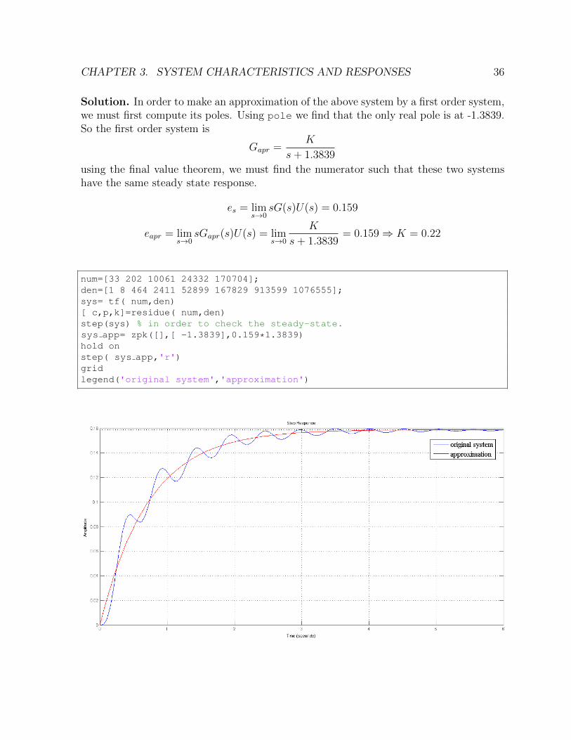
Solution. In order to make an approximation of the above system by a first order system,we must first compute its poles. Using pole we find that the only real pole is at -1.3839.So the first order system is
Gapr =K
s+ 1.3839
using the final value theorem, we must find the numerator such that these two systemshave the same steady state response.
es = lims→0
sG(s)U(s) = 0.159
eapr = lims→0
sGapr(s)U(s) = lims→0
K
s+ 1.3839= 0.159⇒ K = 0.22
num=[33 202 10061 24332 170704];den=[1 8 464 2411 52899 167829 913599 1076555];sys= tf( num,den)[ c,p,k]=residue( num,den)step(sys) % in order to check the steady-state.sys app= zpk([],[ -1.3839],0.159*1.3839)hold onstep( sys app,'r')gridlegend('original system','approximation')
CHAPTER 3. SYSTEM CHARACTERISTICS AND RESPONSES 37
Example 3.3.7. [Nise, 2013, Linkens, 1992] Anesthesia induces muscle relaxation (paral-ysis) and unconsciousness in the patient. Muscle relaxation can be monitored using elec-tromyogram signals from nerves in the hand; unconsciousness can be monitored using thecardiovascular systems mean arterial pressure. The anesthetic drug is a mixture of isoflu-rane and atracurium. An approximate model relating muscle relaxation to the percentisoflurane in the mixture is
G(s) =P (s)
U(s)=
0.0763
s2 + 1.15s+ 0.28
where P(s) is muscle relaxation measured as a fraction of total paralysis (normalized tounity) and U(s) is the percent mixture of isoflurane.
1. Plot the step response of paralysis if a 2% mixture of isoflurane is used.
2. What percent isoflurane would have to be used for 100% paralysis?
Solution. After we define the system in simulink, we will plot its step response for aninput of u=2%, which is equivalent to a step command of the system with an added gainvalue of 2. For this dosage we observe that the paralysis rises at 54.5%
Now, in order to find the amount of dosage required for complete paralysis, we willuse the final value theorem
pfinal(t) = limt→0
sG(s)U(s) = 1
limt→0
sks
0.0763s2+1.15s+0.28
= 1k0.0763
0.28= 1
k = 3.67%
So a dosage of 3.67% is required for full paralysis. Now we will plot the two responses inMatlab and verify the results.
sys=tf([0.0763],[1 1.15 0.28])step(2*sys) % first dosagehold allstep(3.67*sys) % second dosagelegend('2% dosage','3.67% dosage')

CHAPTER 3. SYSTEM CHARACTERISTICS AND RESPONSES 38
Chapter 4
Dynamic Behavior of First-Orderand Second-Order Systems
We shall begin by describing some basic features of first-order and second-order systemsand then we will give examples of them.
4.1 First-Order and Second-Order System’s Features
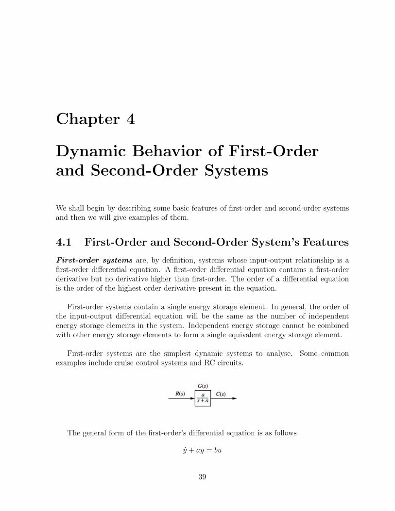
First-order systems are, by definition, systems whose input-output relationship is afirst-order differential equation. A first-order differential equation contains a first-orderderivative but no derivative higher than first-order. The order of a differential equationis the order of the highest order derivative present in the equation.
First-order systems contain a single energy storage element. In general, the order ofthe input-output differential equation will be the same as the number of independentenergy storage elements in the system. Independent energy storage cannot be combinedwith other energy storage elements to form a single equivalent energy storage element.
First-order systems are the simplest dynamic systems to analyse. Some commonexamples include cruise control systems and RC circuits.
The general form of the first-order’s differential equation is as follows
y + ay = bu
39

CHAPTER 4. DYNAMIC BEHAVIOROF FIRST-ORDER AND SECOND-ORDER SYSTEMS40
The first-order’s transfer function is
G(s) =b
s+ a
Second-order systems are commonly encountered in practice, and are the simplesttype of dynamic system to exhibit oscillations. In fact many real higher order systemsare modelled as second-order to facilitate analysis. Typical examples are the mass-spring-damper systems and RLC circuits.
The second-order’s transfer function is:
G(s) =ω2n
s2 + 2ζωns+ ω2n
where ωn is natural frequency and ζ the damping ratio. Depending on the value of thedamping ratio the system exhibits different behavior.
ζ = 0 Undamping The system has two imaginary poles. There is no damp-ing
0 < ζ < 1 Under-damping The system has stable imaginary poles. Quickly tendsto equilibrium, but with oscillation
ζ > 1 Over-damping The system has stable real poles. Tends slower to equi-librium, but when it reach, remains in balance
ζ = 1 Critical damping The system has a double real stable pole. Tends tobalance the maximum possible time without oscillation.

CHAPTER 4. DYNAMIC BEHAVIOROF FIRST-ORDER AND SECOND-ORDER SYSTEMS41
The qualitative analysis of first and second order systems regards the characteristicsof the transient response and the steady state errors. The analysis of these characteris-tics helps determine the quality of the response regarding specific design requirements.For example, when controlling the flow of a water tank, we want to stabilize the watercapacity to a steady level before the tank overflows. This in control theory terms is theminimization of the overshoot. If in addition we desire this transition to a specific waterlever to be done in as little time as possible, then we must study the rise and settling timeof the system.
As another example, when we design a remote controlled navigation system, it is ouraim to input specific coordinates for the system to follow. So in this case we want tominimize the difference between input and output, i.e. the steady state error.
Overall, the basic characteristics that we study are the following:Overshoot: Describe the difference in the response of the system between the tran-
sitional and permanent state, when the system is stimulated by the unit step input. Weare interested in the maximum elevation as well as the time it happens.
Rise time: The time required to switch the system’s response (in step input)from10% to 90% of it’s final value.
Settling time: The time needed to switch the system’s response (in step input) andremain within a certain range of the final price (typically ±2%).
Peak time: The time required to reach the first, or maximum peak.
4.2 Examples
Example 4.2.1. Create a program that will plot the step response of the followingtransfer function
G(s) =a
s+ a.
for a=1,2,..5
Solution.
leg=[];for i=1:5
sys=zpk([],[-i],i);hold allstep(sys);line=horzcat('poles= -',num2str(i));leg=strvcat(leg,line);
endlegend(leg)
CHAPTER 4. DYNAMIC BEHAVIOROF FIRST-ORDER AND SECOND-ORDER SYSTEMS42
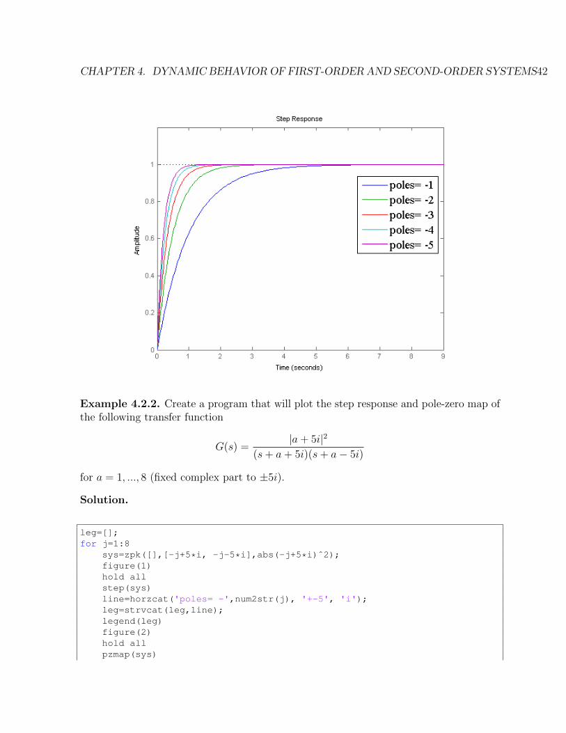
Example 4.2.2. Create a program that will plot the step response and pole-zero map ofthe following transfer function
G(s) =|a+ 5i|2
(s+ a+ 5i)(s+ a− 5i)
for a = 1, ..., 8 (fixed complex part to ±5i).
Solution.
leg=[];for j=1:8
sys=zpk([],[-j+5*i, -j-5*i],abs(-j+5*i)ˆ2);figure(1)hold allstep(sys)line=horzcat('poles= -',num2str(j), '+-5', 'i');leg=strvcat(leg,line);legend(leg)figure(2)hold allpzmap(sys)

CHAPTER 4. DYNAMIC BEHAVIOROF FIRST-ORDER AND SECOND-ORDER SYSTEMS43
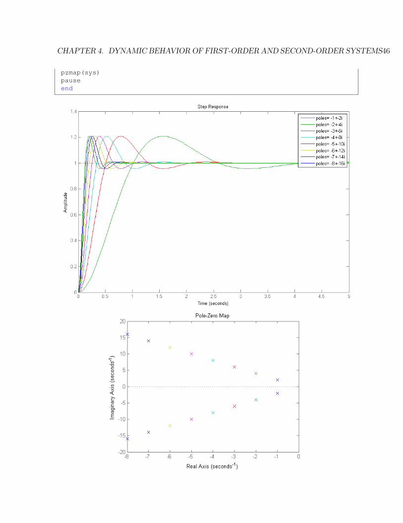
pauseend% Keep pressing enter till you have the desirable result (1-8).

CHAPTER 4. DYNAMIC BEHAVIOROF FIRST-ORDER AND SECOND-ORDER SYSTEMS44
Example 4.2.3. Create a program that will plot the step response and pole-zero map ofthe following transfer function
G(s) =|2 + wi|2
(s+ 2 + wi)(s+ 2− wi)
for w = 1, ..., 8 (constant real part to −2).
Solution.
for j=1:8sys=zpk([],[-2+j*i, -2-j*i],abs(-2+j*i)ˆ2)figure(1)hold allstep(sys)figure(2)hold allpzmap(sys)pause
end

CHAPTER 4. DYNAMIC BEHAVIOROF FIRST-ORDER AND SECOND-ORDER SYSTEMS45
Example 4.2.4. Create a program that will plot the step response and pole-zero map ofthe following transfer function
G(s) =|w + 2wi|2
(s+ w + 2wi)(s+ w − 2wi)
for w = 1, ..., 8.
Solution.
leg=[];for j=1:8
sys=zpk([],[-j+2*j*i, -j-2*j*i],abs(j+2*j*i)ˆ2);figure(1)hold allstep(sys)% In order to create the legend string:line=horzcat('poles= -',num2str(j), '+-', num2str(2*j), 'i');leg=strvcat(leg,line);legend(leg)figure(2)hold all
CHAPTER 4. DYNAMIC BEHAVIOROF FIRST-ORDER AND SECOND-ORDER SYSTEMS46
pzmap(sys)pauseend

Chapter 5
Systems with Delay
5.1 Introduction
Real dynamical systems often show a time lag between the change of an input and thecorresponding change of the output. There is a whole range of reasons that can causethis time lag. Yet for the needs of mathematical modeling, it is aggregated into a totalphenomenon called time delay or dead time. Dead time can be defined as the time intervalbetween the instant when the variation of an input variable is produced and the instantwhen the consequent variation of the output variable starts.
The meaning of delay systems can be understood, considering examples in real life. Afaucet with a handle that controls the temperature of the water can be such an example.Even though the handle is immediately turned to achieve the desired temperature thewater needs time to get to the desired point. Another example is a man crossing a road,when suddenly sees an incoming vehicle. There is a time interval between the momentthe man sees the car and the moment he reacts to avoid getting hit.
5.2 Defining a Delay System in Matlab
There are two basic ways of defining a delay system to matlab, that will be describednext along with the corresponding commands.
5.2.1 Defining a Delay system by its transfer function
The first way is to directly insert the transfer function. This can be done using thecommands:
sys=zpk(z,p,k,'InputDelay',T)sys=tf(num,den,'InputDelay',T)
47
CHAPTER 5. SYSTEMS WITH DELAY 48
The system defined by these commands shall be, when the delay is not 0, the transferfunction of the system without delay defined by the same zeros, poles and gain or samenumerator and denominator when using the first or the second command respectively,multiplied by e−Ts. This is expected considering the following. Suppose a function u(t)is given and the corresponding Laplace transformation is U(s). When u(t) has dead timeT is represented as u(t-T) and the corresponding Laplace transformation is e−TsU(s).
5.2.2 Pade Approximation
The term e−Ts can be approximated using either the Taylor method or the Pade method.Yet the Pade method is more accurate and so it is the most common for this cause.
It is known from basic analysis that the Taylor polynomial of degree n for e−Ts is
1− sT
1!+
(sT )2
2!− · · ·+ (−1)n
(sT )n
n!=
n∑i=0
(−1)i(sT )i
i!
The Taylor approximation uses the fact that e−Ts = e−Ts2
eTs2
. Using this and the Taylor
series of e−Ts one is able to get the approximations. The approximations for degrees 1,2and 3 are given below
Degree n Taylor Approximation1 2−Ts
2+Ts
2 8−4(Ts)+(Ts)2
8+4(Ts)+(Ts)2
3 48−24(Ts)+6(Ts)2−(Ts)3
48+24(Ts)+6(Ts)2+(Ts)3
The Pade approximation uses the fact that
e−Ts ≈m+n∑i=0
(−1)i(Ts)i
i!=
∑mi=0 pi(sT )i∑ni=0 qi(sT )i
where pi = (−1)i (m+n−i)!m!(m+n)!i!(n−i)! for i = 0, 1, ...,m and qi = (−1)i (m+n−i)!n!
(m+n)!i!(m−i)! fori = 0, 1, ..., n. When the degree of the numerator and denominator is the same, Padeapproximation of e−Ts for degree 1, 2 and 3 is given below
Degree n Pade Approximation1 2−Ts
2+Ts
2 12−6(Ts)+(Ts)2
12+6(Ts)+(Ts)2
3 120−60(Ts)+12(Ts)2−(Ts)3
120+60(Ts)+12(Ts)2+(Ts)3
In Matlab, given a defined delay system, named sys, one can use the Pade approxima-tion to define a new system , we will name it sys app, where the exponential factor e−Ts
CHAPTER 5. SYSTEMS WITH DELAY 49
is now replaced with its approximation, using the command: sys app=pade(sys,N),where N is the degree of the approximation. At this point it should be commented thatthis command gives an approximation where the degree of numerator and denominatorare both equal to N.
Another really useful command is [num,den]=pade(T,N). The output of this com-mand is a vector with the numerator and denominator of the Pade approximation fore−Ts of degree N.
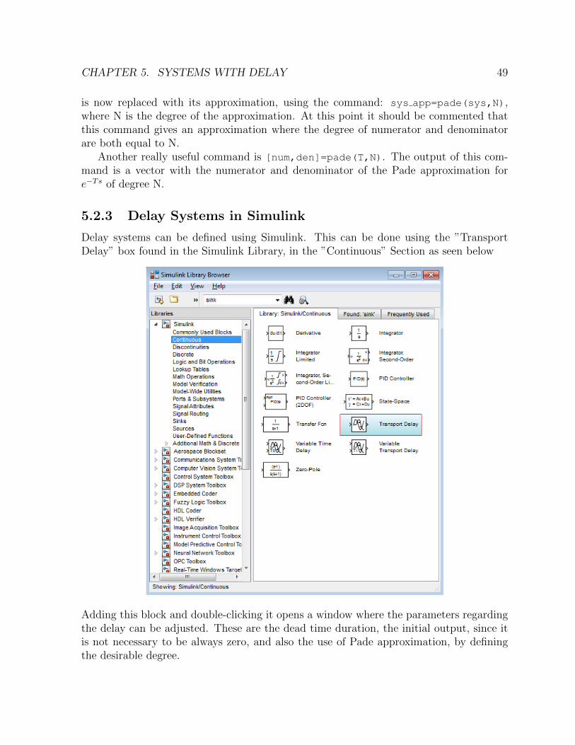
5.2.3 Delay Systems in Simulink
Delay systems can be defined using Simulink. This can be done using the ”TransportDelay” box found in the Simulink Library, in the ”Continuous” Section as seen below
Adding this block and double-clicking it opens a window where the parameters regardingthe delay can be adjusted. These are the dead time duration, the initial output, since itis not necessary to be always zero, and also the use of Pade approximation, by definingthe desirable degree.

CHAPTER 5. SYSTEMS WITH DELAY 50
5.2.4 Example
Example 5.2.1. Suppose a system with transfer function G(s) = 10s2+3s+10
is given.
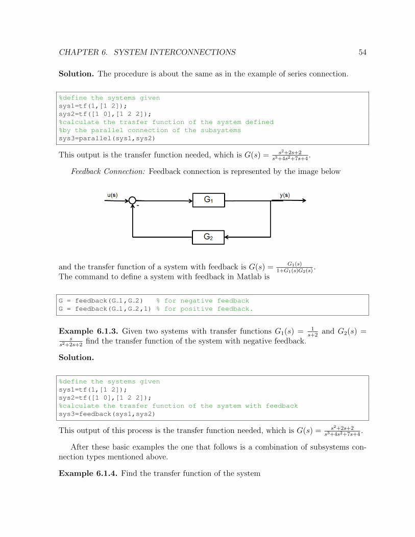
1. Plot the step response for the delay system and its Pade approximations of first andsecond degree.
2. Find the numerator and denominator of e−Ts for the approximations used.
3. Plot the error for the different Pade approximations.
Solution.
%defining the delay systemsys1=tf(10,[1 3 10],'InputDelay',1);%Getting Pade approximations for degrees 1 and 2sys2=pade(sys1,1);sys3=pade(sys1,2);%Getting the graph of all three approximationsfigure;step(sys1,sys2,sys3)title('Delay System and Pade approximations')legend('original','pade 1st order','pade 2nd order')grid
%To see the terms of the approximation for delay 1 we use[num1,den1]=pade(1,1);[num2,den2]=pade(1,2);
%Define e 1 the error of the Pade approximation of degree 1 and%e 2 the error of the Pade approximation of degree 2figure(2);e 1=sys1-sys2;e 2=sys1-sys3;step(e 1,e 2)title('Errors of Pade approximations')legend('error of Pade approx. of deg. 1','error of Pade approx. of deg. 2')grid
This will produce the graph of the original system and the systems with Pade approxi-mations of degree one and two as shown below
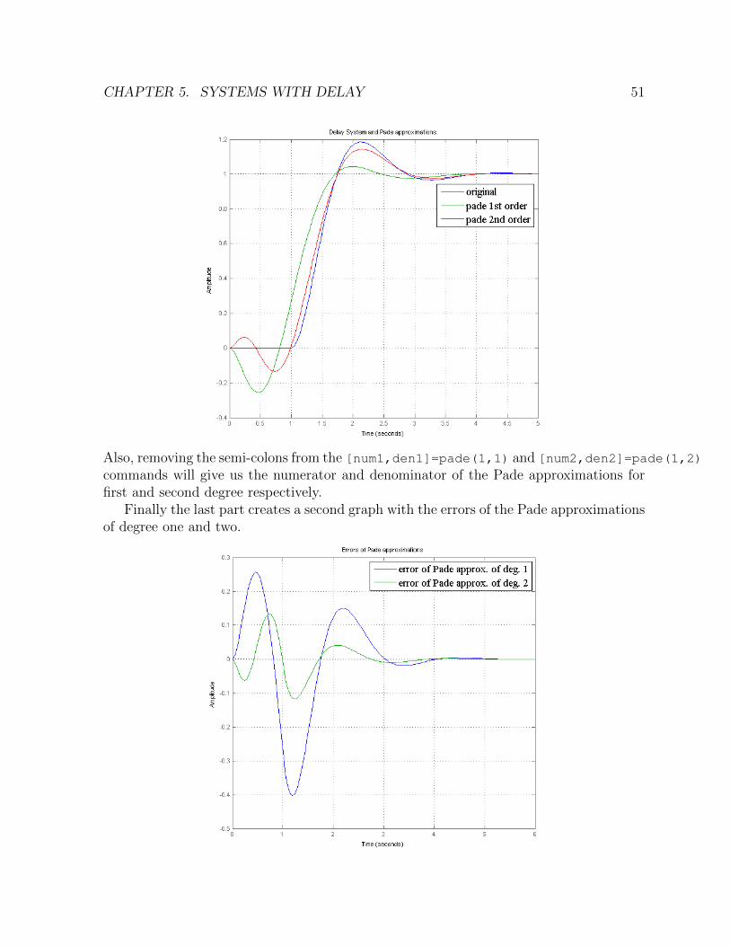
CHAPTER 5. SYSTEMS WITH DELAY 51
Also, removing the semi-colons from the [num1,den1]=pade(1,1) and [num2,den2]=pade(1,2)
commands will give us the numerator and denominator of the Pade approximations forfirst and second degree respectively.
Finally the last part creates a second graph with the errors of the Pade approximationsof degree one and two.

Chapter 6
System Interconnections
6.1 Subsystem Connection Types
Up until this point we studied simple systems. The next step is to define complex sys-tems since these are the most common in applications. Complex systems consist of simplesubsystems connected to each other. There are three different types of subsystem con-nections:
1. Series
2. Parallel
3. Feedback
Of course a complex system can be defined by subsystems connected in a combination ofthe above interconnections.
We shall now observe how each connection type defines the transfer function of thecomplex system. To do so we shall consider two defined systems with transfer functionsG1 and G2 and input u.
Series Connection: This type of connection is represented by the image below
The transfer function of the system defined by this type of connection isG(s) = G1(s)G2(s)The result remains the same regardless of the number of the systems connected. Thetransfer function of a system defined by a series connection of subsystems with transferfunctions G1, G2, · · · , Gn, n ∈ N is G(s) = G1(s)G2(s) · · ·Gn(s). The commands used todefine a system of this type in Matlab are
52

CHAPTER 6. SYSTEM INTERCONNECTIONS 53
sys=series(G1,G2,. . . ,Gn)sys=G1*G2*. . . *Gn
Example 6.1.1. Given two systems with transfer functions G1(s) = 1s+2
and G2(s) =s
s2+2s+2find the transfer function of the system defined by the two cascaded subsystems.
Solution. The system shall look like this
%define the systems givensys1=tf(1,[1 2]);sys2=tf([1 0],[1 2 2]);%calculate the trasfer function of the system defined by the cascaded ...
systemssys3=series(sys1,sys2)
This output is the transfer function needed, which is G(s) = ss3+4s2+6s+4
.
Parallel Connection: This kind of connection is represented by the image bellow
and the transfer function of a system defined by the parallel connections of two systemsis H(s) = G1(s) +G2(s).The commands used to define a system as a parallel connection of two subsystems inMatlab are
sys = parallel(G1,G2,. . .,Gn)sys = G1+G2+. . . +Gn
Example 6.1.2. Given two systems with transfer functions G1(s) = 1s+2
and G2(s) =s
s2+2s+2find the transfer function of the system defined by the two subsystems with parallel
connection.
CHAPTER 6. SYSTEM INTERCONNECTIONS 54
Solution. The procedure is about the same as in the example of series connection.
%define the systems givensys1=tf(1,[1 2]);sys2=tf([1 0],[1 2 2]);%calculate the trasfer function of the system defined%by the parallel connection of the subsystemssys3=parallel(sys1,sys2)
This output is the transfer function needed, which is G(s) = s2+2s+2s3+4s2+7s+4
.
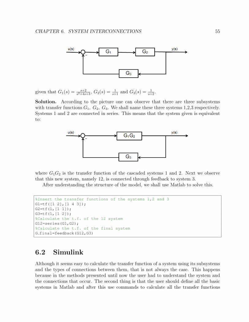
Feedback Connection: Feedback connection is represented by the image below
and the transfer function of a system with feedback is G(s) = G1(s)1+G1(s)G2(s)
.The command to define a system with feedback in Matlab is
G = feedback(G 1,G 2) % for negative feedbackG = feedback(G 1,G 2,1) % for positive feedback.
Example 6.1.3. Given two systems with transfer functions G1(s) = 1s+2
and G2(s) =s
s2+2s+2find the transfer function of the system with negative feedback.
Solution.
%define the systems givensys1=tf(1,[1 2]);sys2=tf([1 0],[1 2 2]);%calculate the trasfer function of the system with feedbacksys3=feedback(sys1,sys2)
This output of this process is the transfer function needed, which is G(s) = s2+2s+2s3+4s2+7s+4
.
After these basic examples the one that follows is a combination of subsystems con-nection types mentioned above.
Example 6.1.4. Find the transfer function of the system
CHAPTER 6. SYSTEM INTERCONNECTIONS 55
given that G1(s) = s+2s2+4s+3
, G2(s) = 1s+1
and G3(s) = 1s+2
.
Solution. According to the picture one can observe that there are three subsystemswith transfer functions G1, G2, G3. We shall name these three systems 1,2,3 respectively.Systems 1 and 2 are connected in series. This means that the system given is equivalentto:
where G1G2 is the transfer function of the cascaded systems 1 and 2. Next we observethat this new system, namely 12, is connected through feedback to system 3.
After understanding the structure of the model, we shall use Matlab to solve this.
%Insert the transfer functions of the systems 1,2 and 3G1=tf([1 2],[1 4 3]);G2=tf(1,[1 1]);G3=tf(1,[1 2]);%Calculate the t.f. of the 12 systemG12=series(G1,G2);%Calculate the t.f. of the final systemG final=feedback(G12,G3)
6.2 Simulink
Although it seems easy to calculate the transfer function of a system using its subsystemsand the types of connections between them, that is not always the case. This happensbecause in the methods presented until now the user had to understand the system andthe connections that occur. The second thing is that the user should define all the basicsystems in Matlab and after this use commands to calculate all the transfer functions
CHAPTER 6. SYSTEM INTERCONNECTIONS 56
needed. This process is more time consuming and difficult depending on the complexityof the system.
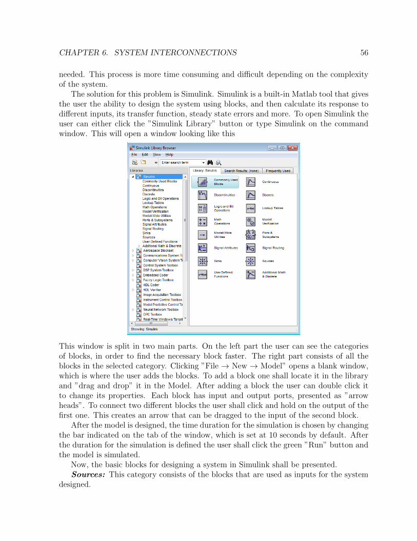
The solution for this problem is Simulink. Simulink is a built-in Matlab tool that givesthe user the ability to design the system using blocks, and then calculate its response todifferent inputs, its transfer function, steady state errors and more. To open Simulink theuser can either click the ”Simulink Library” button or type Simulink on the commandwindow. This will open a window looking like this
This window is split in two main parts. On the left part the user can see the categoriesof blocks, in order to find the necessary block faster. The right part consists of all theblocks in the selected category. Clicking ”File → New → Model” opens a blank window,which is where the user adds the blocks. To add a block one shall locate it in the libraryand ”drag and drop” it in the Model. After adding a block the user can double click itto change its properties. Each block has input and output ports, presented as ”arrowheads”. To connect two different blocks the user shall click and hold on the output of thefirst one. This creates an arrow that can be dragged to the input of the second block.
After the model is designed, the time duration for the simulation is chosen by changingthe bar indicated on the tab of the window, which is set at 10 seconds by default. Afterthe duration for the simulation is defined the user shall click the green ”Run” button andthe model is simulated.
Now, the basic blocks for designing a system in Simulink shall be presented.Sources: This category consists of the blocks that are used as inputs for the system
designed.

CHAPTER 6. SYSTEM INTERCONNECTIONS 57
We shall focus on the blocks that will be of most use during this presentation and theirproperties.
”Step” Block: This represents a step input. The properties for this block include themoment when the value of the step function changes, the initial value and the final value.
”Ramp” Block: This represents a ramp input. The properties for this block includethe gradient of the signal and also the time the signal is produced.
”Sine” Wave: This represents a sinusoidal input. The properties for this block includethe amplitude, frequency and phase for this input.
Sinks: This tab contains the output blocks. We shall focus on two main blocks inthis category.
”Scope” Block: This block creates a diagram of the output signal against and time.To do so the user has to create the desired system and connect it to the Scope block.
”To Workspace” Block: This block allows the user to save the results of the simulationas variables in the workspace. In the options of this block the user can change the name ofthe variable and should also select ”Array” in the ”Save Format” block ( it is ”Timeseries”by default). Finally the user should open the ”Simulation” tab in the model window andthen go to ”Model Configuration Parameters”. On the next window the user shall clickthe ”Data Import/Export” tab and set the ”Format” to ”Array”. This should be done inorder to save the time variable as an array in the workspace.

CHAPTER 6. SYSTEM INTERCONNECTIONS 58
Continuous: This tab contains the blocks needed to insert transfer function subsys-tems.

CHAPTER 6. SYSTEM INTERCONNECTIONS 59
In this tab there are three basic blocks. The ”Transfer Fcn” and the ”Zero-Pole” thatare used to define a transfer function and the ”Transport Delay” that is used to define a”Delay System”.
”Transfer Fcn” Block: This block allows the user to define the transfer function of asystem using the numerator and denominator coefficients.
”Zero-Pole” Block: This block is also used to define a transfer function but this timethe data needed are the zeros and poles of the system. In the options of this block theuser can also adjust the gain.
”Transport Delay” Block: This block is used to define a delay system. The user shallplace this block in series to a transfer function block.In the options the user can changethe dead time and the initial value for the system.
Math Operators: Although this tab contains many useful blocks we shall focus ontwo of them, that are the most important for the purposes of this book. These are the”Gain” and ”Sum” blocks.
”Gain” block: This block is used when the user needs to multiply with a real coefficient.This real number is defined in the options.
”Sum” block: This block is used to add different signals. It is used to create parallelconnections of subsystems and also for feedback. In its options the user can select theshape of the block (it is a circle by default) and also the number of the signals added
CHAPTER 6. SYSTEM INTERCONNECTIONS 60
along with their sign. In the ”list of signs” section the user can use the ”|” symbol toorganize the space between the input ports.
6.3 Examples
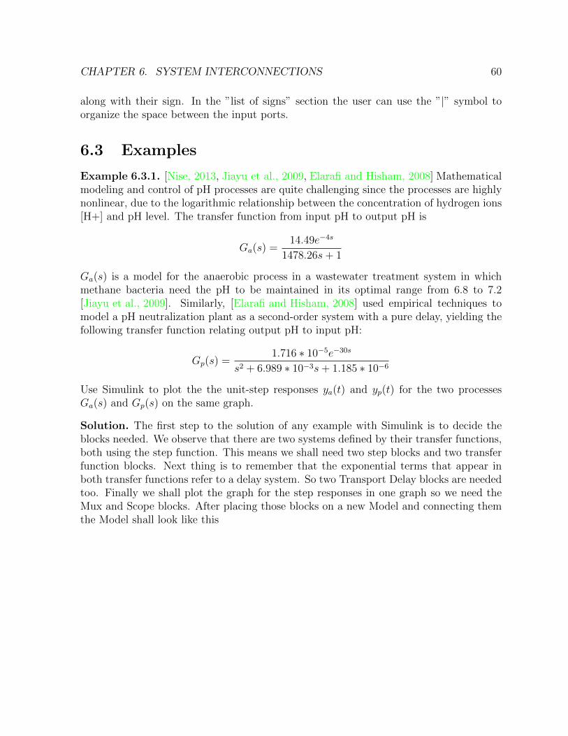
Example 6.3.1. [Nise, 2013, Jiayu et al., 2009, Elarafi and Hisham, 2008] Mathematicalmodeling and control of pH processes are quite challenging since the processes are highlynonlinear, due to the logarithmic relationship between the concentration of hydrogen ions[H+] and pH level. The transfer function from input pH to output pH is
Ga(s) =14.49e−4s
1478.26s+ 1
Ga(s) is a model for the anaerobic process in a wastewater treatment system in whichmethane bacteria need the pH to be maintained in its optimal range from 6.8 to 7.2[Jiayu et al., 2009]. Similarly, [Elarafi and Hisham, 2008] used empirical techniques tomodel a pH neutralization plant as a second-order system with a pure delay, yielding thefollowing transfer function relating output pH to input pH:
Gp(s) =1.716 ∗ 10−5e−30s
s2 + 6.989 ∗ 10−3s+ 1.185 ∗ 10−6
Use Simulink to plot the the unit-step responses ya(t) and yp(t) for the two processesGa(s) and Gp(s) on the same graph.
Solution. The first step to the solution of any example with Simulink is to decide theblocks needed. We observe that there are two systems defined by their transfer functions,both using the step function. This means we shall need two step blocks and two transferfunction blocks. Next thing is to remember that the exponential terms that appear inboth transfer functions refer to a delay system. So two Transport Delay blocks are neededtoo. Finally we shall plot the graph for the step responses in one graph so we need theMux and Scope blocks. After placing those blocks on a new Model and connecting themthe Model shall look like this

CHAPTER 6. SYSTEM INTERCONNECTIONS 61
Next thing is to run the simulation and open the scope block to see the common graphfor these two transfer functions. Running the simulation for 12,000 seconds and autoscaleon the graph, the result is the following:
Chapter 7
State Space Systems
7.1 Introduction
The state space approach, also referred to as the modern, or time-domain approach, is amethod for modelling, analysing and designing a wide range of both linear and non-linearsystems. State space models use state variables to describe a system by a set of first-order differential equations. In this chapter, we will present methods for creating a statespace model, ways to convert between state space and transfer function and show how tocalculate various systems’ responses.
7.2 State space representation
A system is represented in state space by the following equations:
x′(t) = Ax(t) +Bu(t)
y(t) = Cx(t) +Du(t)
where:
• x(t) : State vector• u(t) : Input/control vector• y(t) : Output vector• A ∈ Rn×n : System matrix. It relates how the current state affects the state changex′
• B ∈ Rn×m : Input/control matrix. It determines how the system input affects thestate change
• C ∈ Rl×n : Output matrix. Determines the relationship between the system stateand the system output
• D ∈ Rl×m : Feedthrough/feedforward matrix. Allows the system input to affectthe system output directly
62
CHAPTER 7. STATE SPACE SYSTEMS 63
The first equation is called the state equation and the second the output equation.
In order to create a state space system, we need to know the matrices A,B,C,D. Wecan define a state space system by using the function
sys = ss(A,B,C,D)
Given that we have already defined our state space system in the workspace as we didwith the above command, we can extract matrices A,B,C,D using
[A,B,C,D]=ssdata(sys) % Returns matrices A,B,C,D
We can convert from a transfer function to a state space system, in other words, if wehave a transfer function, we can find the state space representation that corresponds tothis transfer function. To achieve this use
[A,B,C,D] = tf2ss(num,den);sys = ss(A,B,C,D)
Function tf2ss(num,den) returns matrices A,B,C,D. Note that, we have to assign 4output variables, in this case A,B,C,D, otherwise Matlab will not return the completeresult. Then, we create the state space model with the command ss.
An alternative way of converting to a state space model from a transfer function, isby using
sys ss = ss(sys)
provided that, we have already stored the transfer function inside the variable sys. Thismethod though has a disadvantage, since the matrices A,B,C,D are not saved as variablesin the workspace. On the other hand, in order to convert from a state space model to atransfer function, we can use
[num,den] = ss2tf(A,B,C,D);sys = tf(num,den)
Function ss2tf(A,B,C,D) returns the numerator and the denominator of the transferfunction. Then, we create the transfer function with the command tf.
In case we have multiple inputs or outputs in our system and therefore the transferfunction is a matrix, the function
[num,den] = ss2tf(A,B,C,D,n)
CHAPTER 7. STATE SPACE SYSTEMS 64
returns the numerator and denominator of the transfer function that results when then-th input of our system is excited by a unit impulse.
Alternatively, if we have already defined our system in state space form inside thevariable sys we can use
sys tf = tf(sys)
In a similar way, one can use the following commands:
[A,B,C,D] = zp2ss(z,p,k);sys = ss(A,B,C,D)
Converts a zero-pole-gain model, to a state space model.
[z,p,k] = ss2zp(A,B,C,D,i);sys = zpk(z,p,k)
Converts a state space model, to a zero-pole-gain model, from the i -th input(using thei -th columns of B and D).
Generally, for systems with multiple inputs and outputs, the conversion from a statespace model to a transfer function is easier when using the command tf(sys) or zpk(sys)than ss2tf(A,B,C,D,ni) or ss2zp(A,B,C,D,i), due to the fact that such a systemwill be represented by more than one transfer functions and the above commands onlyproduce the numerators and denominators of the transfer function. Therefore it’s up tothe user to extract the different combinations of numerators and denominators to createall the transfer functions that represent the system. On the other hand, commands liketf(sys) and zpk(sys), return all the transfer functions that represent the system in astraightforward way.
7.2.1 Examples
Example 7.2.1. Consider the following transfer function
G(s) =s+ 1
s2 + 2s+ 1
Find the state space model, that corresponds to this transfer function.
Solution.
num = [1 1];den = [1 2 1];
[A,B,C,D] = tf2ss(num,den); % Convert from tf to ss.sys = ss(A,B,C,D)

CHAPTER 7. STATE SPACE SYSTEMS 65
Example 7.2.2. Consider the following transfer function
K(s) =s
2s2 + 3s+ 1
Find the state space model, that corresponds to this transfer function.
Solution.
num = [1 0];den = [2 3 1];sys tf = tf(num,den)
sys ss = ss(sys tf) % Convert from tf to ss
% Note, that in this way matrices A,B,C,D are not saved in the workspace.
Example 7.2.3. Consider the following transfer function in factored form
K(s) =2(s− 2)(s− 3)
s(s− 1)
Find the state space model, that corresponds to this transfer function.
Solution.
z = [2 3];p = [0 1];k = 2;[A,B,C,D] = zp2ss(z,p,k)sys = ss(A,B,C,D)
Example 7.2.4. Consider the following state space model
x′(t) =
(2 10 −3
)x(t) +
(21
)u(t)
y(t) =(1 1
)x(t)
Find the zero-pole-gain model, that corresponds to this state space model.
Solution.
A = [2 1;0 -3];B = [2;1];C = [1 1];D = 0;[z,p,k] = ss2zp(A,B,C,D)% B and D have 1 column, this means ss2zp(A,B,C,D) is the same as ...
ss2zp(A,B,C,D,1)sys = zpk(z,p,k)
CHAPTER 7. STATE SPACE SYSTEMS 66
Example 7.2.5. [Nise, 2013, Cavallo et al., 1992] Given the F4-E military aircraft, nor-mal acceleration an and pitch rate q are controlled by elevator deflection δe on the hor-izontal stabilizers and by canard deflection δc. A commanded deflection δcom, is used toeffect a change in both δe and δc. The state equations describing the effect of δcom on anand q is given byanq
δe
=
−1.702 50.72 263.380.22 −1.418 −31.99
0 0 −14
anqδe
+
−272.06014
δcom
(anq
)=
(1 0 00 1 0
)anqδe
Find the transfer functions that correspond to this state space system.
Solution.
A = [-1.702 50.72 263.38;0.22 -1.418 -31.99;0 0 -14];B = [-272.06;0;14];C = [1 0 0;0 1 0];D = [0;0];sys ss = ss(A,B,C,D);sys zpk = zpk(sys ss)
Matlab returns the following transfer functions:
(1) :−272.06(s2 + 1.865s+ 84.13)
(s+ 4.903)(s+ 14)(s− 1.783)
(2) :−507.71(s+ 1.554)
(s+ 4.903)(s+ 14)(s− 1.783)
We get this result because our system has 1 input and 2 outputs.
Transfer function (1) describes the relation between the input and the first output.
Transfer function (2) describes the relation between the input and the second output.
Example 7.2.6. [Nise, 2013, Liceaga-Castro and van der Molen, 1995] An autopilot is tobe designed for a submarine to maintain a constant depth under severe wave disturbances.It has been shown that the system’s linearised dynamics under neutral buoyancy and ata given constant speed are given by:
wqz
θ
=
−0.038 0.896 0 0.00150.0017 −0.092 0 −0.0056
1 0 0 −3.0860 1 0 0
wqzθ
+
−0.0075 −0.0230.0017 −0.0022
0 00 0
(δBδS)

CHAPTER 7. STATE SPACE SYSTEMS 67
(zθ
)=
(0 0 1 00 0 0 1
)wqzθ
where,
• w : The heave velocity• q : The pitch rate• z : The submarine depth• θ : The pitch angle• δB : The bow hydroplane angle• δS : The stern hydroplane angle
(For an explanatory image, please check out the references). Find the transfer functionthat corresponds to this state space system.
Solution.
A = [-0.038 0.896 0 0.0015;0.0017 -0.092 0 -0.0056;1 0 0 -3.086;0 1 0 0];B = [-0.0075 -0.023;0.0017 -0.0022;0 0;0 0];C = [0 0 1 0;0 0 0 1];D = zeros(2);sys = ss(A,B,C,D);sys tf = tf(sys)
Matlab returns 4 transfer functions, because we have 2 inputs and 2 outputs in oursystem. These are the following:
From input 1 to output...-0.0075 sˆ2 - 0.004413 s - 0.0001995
1: -------------------------------------------sˆ4 + 0.13 sˆ3 + 0.007573 sˆ2 + 0.0002103 s
0.0017 s + 5.185e-052: ---------------------------------------
sˆ3 + 0.13 sˆ2 + 0.007573 s + 0.0002103
From input 2 to output...-0.023 sˆ2 + 0.002702 s + 0.0002466
1: -------------------------------------------sˆ4 + 0.13 sˆ3 + 0.007573 sˆ2 + 0.0002103 s
-0.0022 s - 0.00012272: ---------------------------------------
sˆ3 + 0.13 sˆ2 + 0.007573 s + 0.0002103
Continuous-time transfer function.

CHAPTER 7. STATE SPACE SYSTEMS 68
Example 7.2.7. [Nise, 2013, Tari et al., 2005] In the past, Type-1 diabetes patients hadto inject themselves with insulin three to four times a day. New delayed-action insulinanalogues such as insulin Glargine require a single daily dose. For a specific patient,state-space model matrices are given by
x′(t) =
−0.435 0.209 0.020.268 −0.394 00.227 0 −0.02
x(t) +
100
u(t)
y(t) =(0.0003 0 0
)x(t)
where the state variables, input and output are:
• x1 : Insulin amount in plasma compartment• x2 : Insulin amount in liver compartment• x3 : Insulin amount in interstitial (in body tissue) compartment• u : External insulin flow• y : Plasma insulin concentration
Find the system’s transfer function.
Solution.
A = [-0.435 0.209 0.02;0.268 -0.394 0;0.227 0 -0.02];B = [1;0;0];C = [0.0003 0 0];D = 0;[num,den] = ss2tf(A,B,C,D);sys = tf(num,den)
The resulting transfer function is
G(s) =0.0003s2 + 0.0001242s+ 2.364e− 06
s3 + 0.849s2 + 0.1274s+ 0.0005188

Chapter 8
Pole Placement
8.1 Introduction
In the present Chapter, we will present examples of the Pole Placement technique. It isknown that when the system is controllable, the poles of the closed loop system can beplaced at any desired point using an appropriate feedback gain matrix. In the following,we present an analysis of the procedure and more importantly, the commands we aregoing to use, like k=place(A,B,P).
8.2 Basic definitions and functions
Before we proceed to the pole placement technique, first we need to give some importantdefinitions regarding the stability, controllability and stabilizability of a system.
Asymptotic Stability: A system is asymptotically stable if the eigenvalues of thematrix A (or the poles of the system) are located in the left-half of the complex plane.
Critical Stability: A system is critically stable, if at least one single eigenvalue ofthe matrix A (or a pole of the system) is located on the imaginary axis and no pole islocated in the right-half plane of complex numbers. In addition, no poles with multiplicitymore than one are located on the imaginary axis.
Instability: A system is unstable if at least one eigenvalue of the matrix A (or a poleof the system) is located in the right-half complex plane, or poles with multiplicity higherthan one are located on the imaginary axis.
Controllability: A system is considered to be controllable, if for every initial condi-tion x(0) 6= 0 and time t1 > 0, there exists an input signal u(t) and time t1, such that thestate of the system can be driven to the origin in finite time, i.e. x(t1) = 0.
Stabilizability: A system is considered to be stabilizable, if for each initial stateξ ∈ Rn, there exists a control input u(t), such that the state response with initial condition
69

CHAPTER 8. POLE PLACEMENT 70
x(0) = ξ satisfies, limx→∞
x(t) = 0
In other words, when a system is stabilizable, it means that we can make it stable.Additionaly, when a system is controllable, it is stabilizable. As you will see, in thefollowing examples when we need to perform the pole placement technique in order tomake a system stable or change it’s response, we first examine whether the system iscontrollable or not. If it is controllable, it means that it’s stabilizable and thereforewe can perform the pole placement technique in order to make it stable or change it’sresponse.
In order to examine whether our system is stable, we have to calculate the eigenvaluesof matrix A. Given that we have already defined the matrix A in the workspace, we canachieve that by using the command
eigs = eig(A)
Alternatively, given that we have already defined our system in the workspace insidevariable sys (and not just matrix A) we can use the command
isstable(sys)
Matlab then returns a logical value of whether 1 or 0, where 1 means ”True” and 0 means”False”.
A n-th order system is controllable, if the controllability matrix
Q =(B AB . . . An−1B
)has full rank, i.e. rank(Q) = n. We can examine the controllability of a system by using
Q = ctrb(A,B); % Returns matrix Qrank(Q)
Function ctrb(A,B) returns the controllability matrix Q. Then, using the functionrank(Q) we find the rank of the matrix and if it’s in full rank, our system is controllable.
Alternatively, given that we have already defined our system in the workspace we canuse
Q = ctrb(sys); % Returns matrix Qrank(Q)

CHAPTER 8. POLE PLACEMENT 71
8.3 Pole placement through state feedback
Consider the following state space system
x(t) = Ax(t) +Bu(t)
y(t) = Cx(t)
We define a new input u(t) of the form, u(t) = −Kx(t) + r(t), where
K =(k0 k1 . . . kn−1
)∈ R1×n
is the feedback gain matrix and r(t) is a new input signal. Thus,
u(t) = −(k0 k1 . . . kn−1
)x1
x2...xn
+ r(t)⇒
u(t) = −k0x1 − k1x2 − · · · − kn−1xn + r(t)
This is called state feedback. As you can see we feed back to the input u(t) the statesx1, . . . xn multiplied by the elements of matrix K, which are called gains. By replacing u(t)in our state space equation we get x(t) = Ax(t)+B[−Kx(t)+r(t)] = (A−BK)x(t)+Br(t).The state space system has the following form:
x(t) = (A−BK)x(t) +Br(t)
y(t) = Cx(t)
Now, system stability depends on the location of the eigenvalues of matrix A − BK.Our purpose is to find the appropriate gains, in other words matrix K, in order to havethe desired placement of the eigenvalues (of matrix A − BK). Of course this placementwill take place in the left-half plane of the complex numbers, in order for our system tobe stable.
State space system representation without state feedback
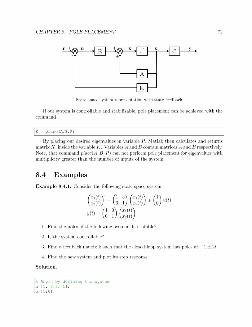
CHAPTER 8. POLE PLACEMENT 72
State space system representation with state feedback
If our system is controllable and stabilizable, pole placement can be achieved with thecommand
K = place(A,B,P)
By placing our desired eigenvalues in variable P , Matlab then calculates and returnsmatrixK, inside the variableK. Variables A andB contain matrices A andB respectively.Note, that command place(A,B, P ) can not perform pole placement for eigenvalues withmultiplicity greater than the number of inputs of the system.
8.4 Examples
Example 8.4.1. Consider the following state space system(x1(t)x2(t)
)′=
(1 33 1
)(x1(t)x2(t)
)+
(10
)u(t)
y(t) =
(1 00 1
)(x1(t)x2(t)
)1. Find the poles of the following system. Is it stable?
2. Is the system controllable?
3. Find a feedback matrix k such that the closed loop system has poles at −1± 2i.
4. Find the new system and plot its step response.
Solution.
% Begin by defining the systema=[1, 3;3, 1];b=[1;0];
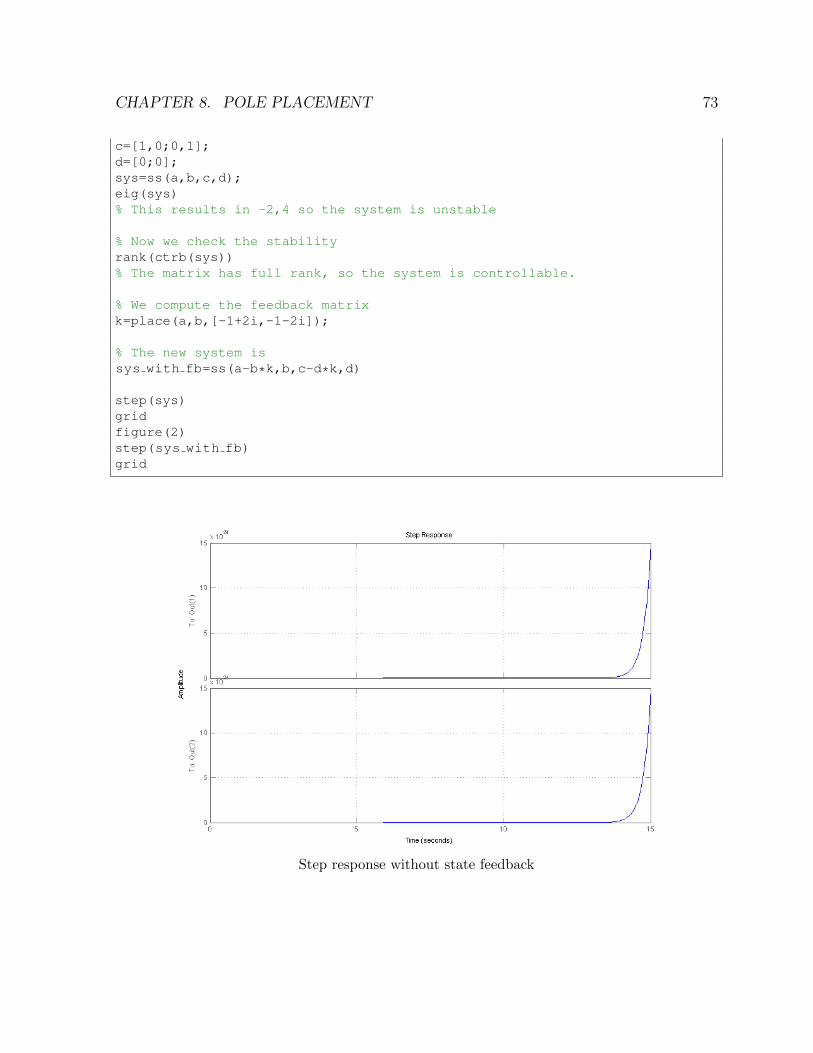
CHAPTER 8. POLE PLACEMENT 73
c=[1,0;0,1];d=[0;0];sys=ss(a,b,c,d);eig(sys)% This results in -2,4 so the system is unstable
% Now we check the stabilityrank(ctrb(sys))% The matrix has full rank, so the system is controllable.
% We compute the feedback matrixk=place(a,b,[-1+2i,-1-2i]);
% The new system issys with fb=ss(a-b*k,b,c-d*k,d)
step(sys)gridfigure(2)step(sys with fb)grid
Step response without state feedback
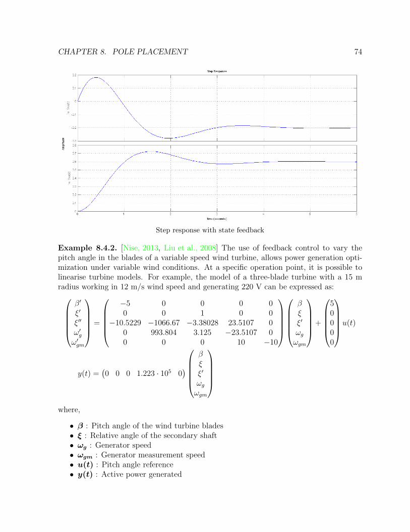
CHAPTER 8. POLE PLACEMENT 74
Step response with state feedback
Example 8.4.2. [Nise, 2013, Liu et al., 2008] The use of feedback control to vary thepitch angle in the blades of a variable speed wind turbine, allows power generation opti-mization under variable wind conditions. At a specific operation point, it is possible tolinearise turbine models. For example, the model of a three-blade turbine with a 15 mradius working in 12 m/s wind speed and generating 220 V can be expressed as:
β′
ξ′
ξ′′
ω′gω′gm
=
−5 0 0 0 00 0 1 0 0
−10.5229 −1066.67 −3.38028 23.5107 00 993.804 3.125 −23.5107 00 0 0 10 −10
βξξ′
ωgωgm
+
50000
u(t)
y(t) =(0 0 0 1.223 · 105 0
)
βξξ′
ωgωgm
where,
• β : Pitch angle of the wind turbine blades• ξ : Relative angle of the secondary shaft• ωg : Generator speed• ωgm : Generator measurement speed• u(t) : Pitch angle reference• y(t) : Active power generated
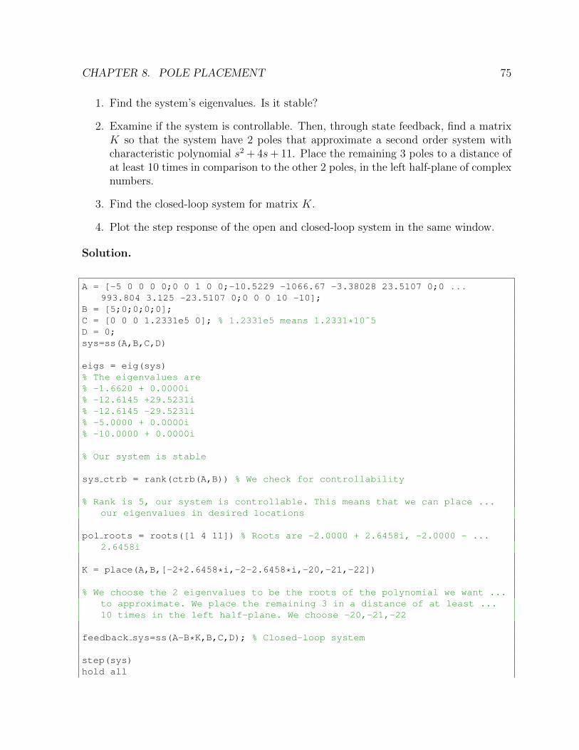
CHAPTER 8. POLE PLACEMENT 75
1. Find the system’s eigenvalues. Is it stable?
2. Examine if the system is controllable. Then, through state feedback, find a matrixK so that the system have 2 poles that approximate a second order system withcharacteristic polynomial s2 + 4s+ 11. Place the remaining 3 poles to a distance ofat least 10 times in comparison to the other 2 poles, in the left half-plane of complexnumbers.
3. Find the closed-loop system for matrix K.
4. Plot the step response of the open and closed-loop system in the same window.
Solution.
A = [-5 0 0 0 0;0 0 1 0 0;-10.5229 -1066.67 -3.38028 23.5107 0;0 ...993.804 3.125 -23.5107 0;0 0 0 10 -10];
B = [5;0;0;0;0];C = [0 0 0 1.2331e5 0]; % 1.2331e5 means 1.2331*10ˆ5D = 0;sys=ss(A,B,C,D)
eigs = eig(sys)% The eigenvalues are% -1.6620 + 0.0000i% -12.6145 +29.5231i% -12.6145 -29.5231i% -5.0000 + 0.0000i% -10.0000 + 0.0000i
% Our system is stable
sys ctrb = rank(ctrb(A,B)) % We check for controllability
% Rank is 5, our system is controllable. This means that we can place ...our eigenvalues in desired locations
pol roots = roots([1 4 11]) % Roots are -2.0000 + 2.6458i, -2.0000 - ...2.6458i
K = place(A,B,[-2+2.6458*i,-2-2.6458*i,-20,-21,-22])
% We choose the 2 eigenvalues to be the roots of the polynomial we want ...to approximate. We place the remaining 3 in a distance of at least ...10 times in the left half-plane. We choose -20,-21,-22
feedback sys=ss(A-B*K,B,C,D); % Closed-loop system
step(sys)hold all

CHAPTER 8. POLE PLACEMENT 76
step(feedback sys)legend('original system','after state feedback')grid
Chapter 9
Observer Design
9.1 Introduction
Suppose a linear, time invariant siso system S is given. Let S be defined by
x(t) = Ax(t) +Bu(t)
y(t) = Cx(t)
where A ∈ Rn×n, B ∈ Rn×1, C ∈ R1×n.For this system the input u(t) is considered a known signal with u(t) = 0 for t ≤ 0.
In addition, we usually also assume that the output and state vectors y(t),x(t) are knownand can be measured for all t ≥ 0. This makes it possible (as was seen in the previouschapter) to apply state feedback in order to change the characteristics of the system. Thismay not always be the case though, since in practice, not all states
x(t) =
x1(t)x2(t)
...xn(t)
, t ≥ 0
could be available for feedback. If that is the case, we need to find a way to estimate theunknown states.
In this case, an equivalent system is constructed, called an observer, with the purposeof estimating all the states of the system. The new observer system is characterised bythe same equations, i.e.
˙x(t) = Ax(t) +Bu(t)
y(t) = Cx(t)
In order to ensure that the estimation is accurate, the observer is additionally fed withthe error signal between the outputs, i.e. y(t)− y(t), multiplied by a gain matrix L. The
77
CHAPTER 9. OBSERVER DESIGN 78
new system takes the form
˙x(t) = Ax(t) +Bu(t) + L(y(t)− y(t)
)⇒
˙x = (A− LC)x(t) + Ly(t) +Bu(t)
y(t) = Cx(t)
The use of the output feedback can be understood considering the approximation error.Let ε(t) denote the error of the approximation, i.e. ε(t) = x(t) − x(t). Substituting thevalues of the state and estimated state, we end up with
ε = (A− LC)ε(t)
The solution of this homogeneous linear diff. equation is
e(t) = e(A−LC)te(0)
So it should be obvious that if the feedback matrix L is chosen in order to have a stablesystem matrix (A-LC), the error e(t)→ 0 and the approximation is accurate. In addition,depending on the value of L, we may obtain quicker or slower approximations. For athorough presentation of the procedure of observer design, one may refer to [Ogata, 2009].
9.2 Observer Construction Example
The method used for constructing an observer will be explained through the followingexample.
Example 9.2.1 (Observer Design). Consider the following system(x′1(t)x′2(t)
)=
(−20.6 2
2 −1
)(x1(t)x2(t)
)+
(51
)u(t)
y(t) =(1 1
)(x1(t)x2(t)
)With initial conditions (
x1(0)x2(0)
)=
(11
)1. Is the system stable?
2. Is the system observable?
3. If the system is observable, create an observer with poles at -10, -9.
4. Assuming different initial conditions for the observer, compare the outputs of thetwo systems, their states and the error of the observer approximation, for differentkinds of inputs and verify the estimation of the observer.

CHAPTER 9. OBSERVER DESIGN 79
5. Would the approximation be the same if the observer had poles near the imaginaryaxis, e.g. at -1,-2?
Solution. The first two questions can be answered through Matlab workspace directly.As a reminder, stability is not necessary to create an observer.
%% Defining the Planta=[-20.6 0;0 -1];b=[0;1];c=[1 1];d=0;sys=ss(a,b,c,d);% Now we check the eigenvalues of the system for stabilityeig(sys); %the eigenvalues are both negative so its stable%then we check the observabilityrank(obsv(sys));%the system is observable so we can construct an observer.
Since the system is observable, the observer construction is possible. So moving on toSimulink, we create the following system

CHAPTER 9. OBSERVER DESIGN 80
The above model constitutes of 3 basic parts. The first is the original plant of the systemwith initial conditions [1,1]. The second part is the observer, created above the originalplant and designed with green colour. The error y(t)−y(t) is fed to the observer, multipliedby L. For the observer we choose as initial conditions [0,0]. The third part consists of allthe scopes for the inputs, the outputs and the errors between real and estimated signals.
Before we can simulate the system, we must choose the values for L. This is donethrough the following commands.
%% Observer pole placement at -10 and -9% This observer will lead to a faster approximation of the two statesL T=place(a',c',[-10,-9])L=L T'% (the symmetric system is used for pole placement)
The matrix L is equal to L =(−6.7429 4.1429
)T. Now we are ready to start the
simulation.It should also be noted that we designed the state space systems using only one
differentiator block. This was done by changing the way the signals are interpreted. Thisis possible by choosing ’Matrix Multiplication’ at the Gain blocks and then defining allthe parameters as matrices in the workspace.
The simulation results for the two states and a step input are the following
From these figures we can observe that the estimation becomes accurate for both statesin less that 1 second, which is a satisfying result. This result is independent of the typeof input that we use, see for example for u(t) = 3sin(t):

CHAPTER 9. OBSERVER DESIGN 81
The swiftness of the approximation is due to the fact that the poles of the observer arechosen to be far left on the imaginary axis, making the system’s response fast. If we chosepoles that would still be stable, but closer on the imaginary axis, then the approximationwould take longer time to reach its accuracy. For example if we chose the poles at -1,-2,the result would be the following
and we can see that it take about 4.5 seconds to get the desired result.

Chapter 10
Root Locus Analysis
10.1 Introduction
The Root locus method covered in this chapter, is a very useful tool in system analysis,used to describe qualitatively the performance of a system with feedback when a systemparameter, usually the gain, is changed. For example, we can see the effect of varyinggain upon percent overshoot, settling time and peak time. It can be used as a graphicaldesign technique, in order to find an appropriate gain value to meet some performancerequirements. (For example a specific value of damping ratio.) If the gain adjustmentcannot give us the desired result, an addition of a compensator to the system will benecessary.
10.2 Root Locus method
Root locus is a graphical presentation of the system’s closed-loop poles, as the gain variesbetween zero and infinity. The MATLAB command that produces the root locus diagramis rlocus.
82

CHAPTER 10. ROOT LOCUS ANALYSIS 83
rlocus(sys) Calculates the root locus diagram of the open-loop SISO model sys.This function can be applied to any of the following negative feedbackloops by setting sys appropriately:
Some other useful commands are the following:
sgrid(z,w) Plots a grid of constant damping factor and natural fre-quency lines. The grid is drawn over the root locusdiagram.
sgrid(z,[ ]) Plots a grid of constant damping factor lines,sgrid([ ],w) or a grid of natural frequency lines respectively.[R,K]=rlocus(sys) Returns the vector K of selected gains and the closed-
loop pole locations(vector R) for these gains.sys=feedback(sys1,sys2) Returns a model object sys for the negative feedback
interconnection of model objects sys1 and sys2.
The last command forms the following negative feedback loop:
So if sys2 is a positive number k, we get the transfer function of the closed-loop systemwhen gain value is equal to k.
Lines of constant damping ratio ζ (ζ = cosφ) are radial lines passing through theorigin as shown below. For example, a damping ratio of 0.5 requires that the complex-conjugate poles lie on the lines drawn through the origin making angles of ±60 with thenegative real axis. (If the real part of a pair of complex-conjugate poles is positive, which

CHAPTER 10. ROOT LOCUS ANALYSIS 84
means that the system is unstable, the corresponding ζ is negative.) The damping ratiodetermines the angular location of the poles, while the natural frequency ω determinesthe distance of the pole from the origin. (with circles)
Since the root locus actually showcases the locations of all possible closed-loop poles,from the root locus we can select a gain such that our closed-loop system will performthe way we want. If any of the selected poles are on the right half plane, the closed-loopsystem will be unstable.
As the gain of the open-loop transfer function varies, the characteristic equationchanges. So the closed-loop poles, which are the roots of the characteristic equation,change too. Let’s see a simple example:
Example 10.2.1. We have the transfer function
G(s) =K
s+ 3
The closed-loop transfer function is:
G(s)
1 +KG(s)=
K
s+K + 3
So the characteristic equation is: s+K + 3 = 0 (1+KG(s)=0).If we put K=0 we get a pole at -3, if we put K=1 we get a pole at -4, if we put K=9 weget a pole at -12 e.t.c.We see that as the value of K is increased, the pole moves to the left, and this can beeasily seen with MATLAB. So it is clear that the root locus begins from the closed-looppole at -3 (with zero gain) and goes to minus infinity. (Note that MATLAB does not showthe direction of the movement of the poles. It should be understood that the movementstarts from the poles and ends to the zeros).

CHAPTER 10. ROOT LOCUS ANALYSIS 85
sys=tf([1],[1 3]);[R,K]=rlocus(sys) % Returns the closed-loop pole locations for varied ...
gain valuesr=rlocus(sys,[0,3,9]) % Returns the closed-loop pole locations for gain ...
values 0,3,9 respectivelyrlocus(sys) % Returns the root locus diagram
Example 10.2.2. Find the root locus plot for the transfer function:
G(s) =K
(s+ 1)(s+ 3)
Find the gain value in order to have damping ratio=0.8, and find the closed-loop transferfunction for that value.
Solution.
sys=tf([1],[1 4 3])rlocus(sys)sgrid(0.8,[]) % Plots a grid of constant damping factor lines for z=0.8sys cl=feedback(sys,3.25) % Returns the closed-loop tranfer function ...
when gain is equal to 3.25
The solution can be found from the intersection points of the root locus and the dampingratio lines. Clicking at these points on the root locus, we obtain the corresponding gain,
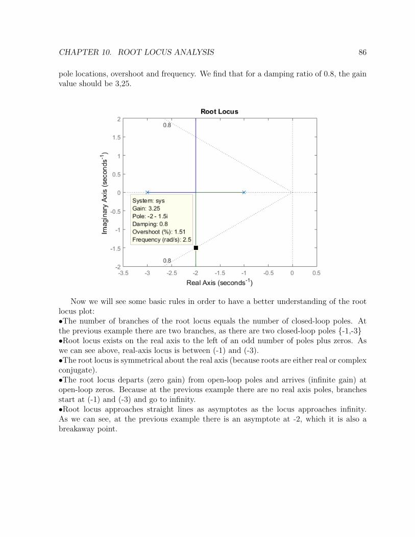
CHAPTER 10. ROOT LOCUS ANALYSIS 86
pole locations, overshoot and frequency. We find that for a damping ratio of 0.8, the gainvalue should be 3,25.
Now we will see some basic rules in order to have a better understanding of the rootlocus plot:•The number of branches of the root locus equals the number of closed-loop poles. Atthe previous example there are two branches, as there are two closed-loop poles -1,-3•Root locus exists on the real axis to the left of an odd number of poles plus zeros. Aswe can see above, real-axis locus is between (-1) and (-3).•The root locus is symmetrical about the real axis (because roots are either real or complexconjugate).•The root locus departs (zero gain) from open-loop poles and arrives (infinite gain) atopen-loop zeros. Because at the previous example there are no real axis poles, branchesstart at (-1) and (-3) and go to infinity.•Root locus approaches straight lines as asymptotes as the locus approaches infinity.As we can see, at the previous example there is an asymptote at -2, which it is also abreakaway point.

CHAPTER 10. ROOT LOCUS ANALYSIS 87
10.3 Examples
Example 10.3.1. Given a negative unity feedback system with the following transferfunction:
G(s) =K(s− 2)(s− 4)
s2 + 6s+ 25
a. Find the root locus diagram.b. For which gain value the closed-loop system becomes stable?c. For which gain value the closed-loop system has poles with damping ratio 0.5? Findthe closed-loop transfer function.d. Find the gain value in order to get frequency value equal to 6.
Solution.
sys=zpk([2 4],[-3+4i -3-4i],1)rlocus(sys)sgrid(0.5,6) % Plots a grid of constant damping ratio lines(z=0.5) and ...
frequency lines(w=6)sys cl=feedback(sys,0.108) % Returns the closed-loop transfer function ...
when the gain value is 0.108
b. As we can see from the root locus diagram, the gain value for which the closed-loopsystem becomes stable is 1. (We click at the intersection points of the root locus and theimaginary axis.)c. Now we click at the intersection points of the loot locus and the damping ratio lines,and we find that the gain value is 0,108.d. There are no gain values which give frequency equal to 6. The reason is that there areno intersection points of the root locus and the frequency lines. This can be clearly seenfrom the pictures below.

CHAPTER 10. ROOT LOCUS ANALYSIS 88
Example 10.3.2. Given a negative unity feedback system with the following transferfunction:
G(s) =K(s+ 1.5)
s(s+ 1)(s+ 10)
a. Find the root locus diagram.b. Find the value of K for which the closed-loop system is stable.c. Find the value of K for which the closed-loop system has overshoot 1.52%.
Solution.
sys=zpk([-1.5],[-1 -10 0],1)rlocus(sys)% Now we will calculate the damping ratio value, when overshoot is 1.52%z=-log(1.52/100)/(sqrt(piˆ2 +log(1.52/100)ˆ2)) % We get that z=0.7998sgrid(0.7998,[]) % Plots a grid of constant damping ratio lines(z=0.7998)
b. Root locus plot is at the left half plane, so the system is stable for all values of K.c. Overshoot is 1.52% when damping ratio is 0, 7998 ' 0, 8. We get the damping ratiolines and as we can see below, the gain values that we want are: 7,32 , 12,7 and 39,6.
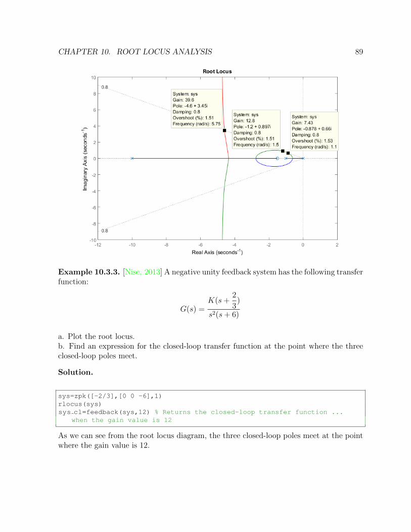
CHAPTER 10. ROOT LOCUS ANALYSIS 89
Example 10.3.3. [Nise, 2013] A negative unity feedback system has the following transferfunction:
G(s) =K(s+
2
3)
s2(s+ 6)
a. Plot the root locus.b. Find an expression for the closed-loop transfer function at the point where the threeclosed-loop poles meet.
Solution.
sys=zpk([-2/3],[0 0 -6],1)rlocus(sys)sys cl=feedback(sys,12) % Returns the closed-loop transfer function ...
when the gain value is 12
As we can see from the root locus diagram, the three closed-loop poles meet at the pointwhere the gain value is 12.

CHAPTER 10. ROOT LOCUS ANALYSIS 90
Example 10.3.4. [Fadali, 2015] Find the root locus of the unity feedback system withtransfer function:
G(s) =K(s+ 3)(s+ 5)
(s+ 1)(s− 7)
a. Find the gain at break-in and breakaway points.b. Find the closed-loop transfer function when damping ratio value is 0.5c. Find the closed-loop transfer function when frequency is equal to 2.
Solution.
sys=zpk([-3 -5],[-1 7],1)rlocus(sys)sgrid(0.5,[])sys cl=feedback(sys,1.56) % Returns the closed-loop transfer function ...
when the gain value is 1.56sgrid([],2)sys cl=feedback(sys,1)
Root locus starts from the two poles -1,7 and ends at the two zeros -3,-5. So as wecan see below, the gain at the breakaway point is 0,508 and at the break-in point is 31,5.Also we can see that when damping ratio is 0,5 the gain value is 1,56 and when frequencyis 2, the gain value is 1.

CHAPTER 10. ROOT LOCUS ANALYSIS 91
Chapter 11
Nyquist Plot
11.1 Introduction
The Nyquist stability criterion, created by Swedish-American electrical engineer HarryNyquist at Bell Telephone Laboratories in 1932, is a graphical technique for determiningthe stability of a dynamical system. This criterion relates the stability of a closed systemto the open-loop frequency response and open loop pole location. It can tell us how manyclosed-loop poles are in the right half-plane, thus helping determine whether a system isstable or not.
11.2 Nyquist Criterion
A Nyquist diagram is a polar plot of the frequency response function G(iω) in the complexplane, for all real values of ω. It’s a plot of the transfer function, G(s) with s = iω. Thecomplex number G(iω), depends upon frequency, so frequency will be the free parameterwhen plotting the imaginary part of G(iω) against the real part of G(iω). We can easilyget the Nyquist plot in Matlab, using the command nyquist.
92

CHAPTER 11. NYQUIST PLOT 93
nyquist(sys) Creates the Nyquist plot of the dynamic systemsys, as the frequency takes values from zero toinfinity. The model can be continuous or discrete.
nyquist(sys,w) Specifies the frequency range or frequency pointsto be used for the plot. To focus on a particularfrequency interval, set w = [wmin, wmax]. To useparticular frequency points, set w to the vector ofdesired frequencies.
nyquist(sys1,sys2,..,sysk) Plots the Nyquist diagrams of several models ona single figure. All systems must have the samenumber of inputs and outputs, but may otherwisebe a mix of continuous and discrete-time systems.We can also specify a distinctive color, linestyle,or marker for each system plot with the syntaxnyquist(sys1,'PlotStyle1',..).
[re,im]=nyquist(sys,w) Returns the real and imaginary parts of the fre-quency response, at the specified frequency w.
An example of a Nyquist plot will illustrate what a Nyquist plot is. We will take a verysimple system:
G(s) =1
s+ 1.
If we substitute s = iw, we get G(iw) =1
iw + 1, and that’s a complex number. We will
compute the real and imaginary parts of G(iw) by converting the denominator to a real
number: G(iw) =1
(iw + 1)
1− iw(1− iw)
=1− iw1 + w2
.
The real and imaginary parts of the frequency response function are:
Re(G(iw)) =1
1 + w2Im(G(iw)) =
−w1 + w2
The Nyquist diagram starts at the point (1,0) at an angle of 0 degrees. As w variesbetween zero and infinity, we get the Nyquist plot as shown below, in the direction ofincreasing w.
sys=tf([1],[1 1])nyquist(sys)% Plots the Nyquist diagram[re,im]=nyquist(sys,2) % Returns the real and imaginary parts of the ...
frequency response, when w=2. The real part is equal to 0.2 and the ...imaginary part is -0.4

CHAPTER 11. NYQUIST PLOT 94
Consider now the following negative feedback system:
We know that the poles of the open-loop system G(s)H(s) are also the poles of 1+G(s)H(s).We can take a random system and easily see that in MATLAB.
sys=tf([1 3 5 7],[2 4 6 8 2]); % We take a random open-loop transfer ...function
pzmap(sys) % Map the poles and zeros for the OL (open-loop) systemfigure; pzmap(sys+1) % Map the poles and zeros for the 1+OL systemclose allnyquist(sys,sys+1) % Plots the Nyquist diagram for both systems
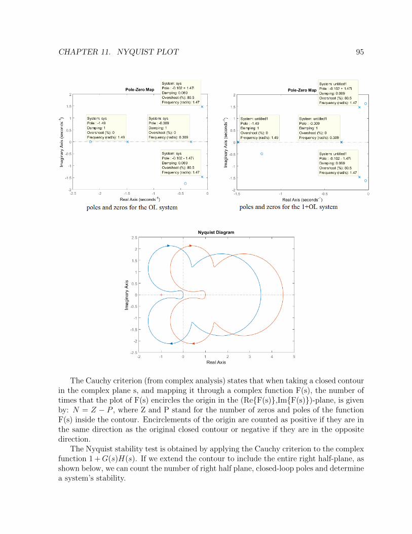
CHAPTER 11. NYQUIST PLOT 95
The Cauchy criterion (from complex analysis) states that when taking a closed contourin the complex plane s, and mapping it through a complex function F(s), the number oftimes that the plot of F(s) encircles the origin in the (ReF(s),ImF(s))-plane, is givenby: N = Z − P , where Z and P stand for the number of zeros and poles of the functionF(s) inside the contour. Encirclements of the origin are counted as positive if they are inthe same direction as the original closed contour or negative if they are in the oppositedirection.
The Nyquist stability test is obtained by applying the Cauchy criterion to the complexfunction 1 +G(s)H(s). If we extend the contour to include the entire right half-plane, asshown below, we can count the number of right half plane, closed-loop poles and determinea system’s stability.
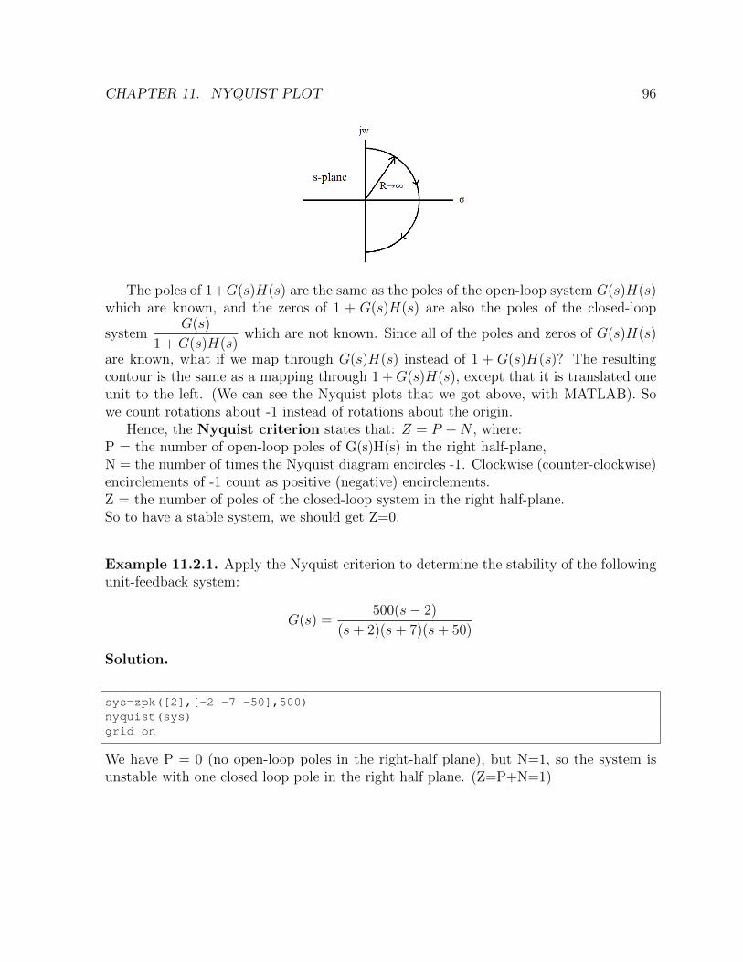
CHAPTER 11. NYQUIST PLOT 96
The poles of 1+G(s)H(s) are the same as the poles of the open-loop system G(s)H(s)which are known, and the zeros of 1 + G(s)H(s) are also the poles of the closed-loop
systemG(s)
1 +G(s)H(s)which are not known. Since all of the poles and zeros of G(s)H(s)
are known, what if we map through G(s)H(s) instead of 1 + G(s)H(s)? The resultingcontour is the same as a mapping through 1 +G(s)H(s), except that it is translated oneunit to the left. (We can see the Nyquist plots that we got above, with MATLAB). Sowe count rotations about -1 instead of rotations about the origin.
Hence, the Nyquist criterion states that: Z = P +N , where:P = the number of open-loop poles of G(s)H(s) in the right half-plane,N = the number of times the Nyquist diagram encircles -1. Clockwise (counter-clockwise)encirclements of -1 count as positive (negative) encirclements.Z = the number of poles of the closed-loop system in the right half-plane.So to have a stable system, we should get Z=0.
Example 11.2.1. Apply the Nyquist criterion to determine the stability of the followingunit-feedback system:
G(s) =500(s− 2)
(s+ 2)(s+ 7)(s+ 50)
Solution.
sys=zpk([2],[-2 -7 -50],500)nyquist(sys)grid on
We have P = 0 (no open-loop poles in the right-half plane), but N=1, so the system isunstable with one closed loop pole in the right half plane. (Z=P+N=1)

CHAPTER 11. NYQUIST PLOT 97
If the open-loop system contains a variable gain K, we set K=1 and sketch the Nyquistdiagram. We consider the critical point to be at - 1
Krather than at -1, and then we adjust
the value of K to yield stability, based upon the Nyquist criterion.Using MATLAB is very easier to determine stability. Using the Nyquist diagram, we
define two quantitative measures of how stable a system is. These quantities are calledgain margin and phase margin. The gain margin is the change in open-loop gain, expressedin decibels (dB), required at 180 degrees of phase shift to make the closed-loop systemunstable. The phase margin is the change in open-loop phase shift required at unity gainto make the closed-loop system unstable. In MATLAB we can find their values usingthe command allmargin. We can also find them from the Nyquist diagram. Right-clickin the graph area, select Characteristics and then select All Stability Margins. Let themouse rest on the margin points to read the gain and phase margins. Gain margin isexpressed in decibels, so we convert it using db2mag.
allmargin(sys) Computes the gain margin, phase margin, delay margin and thecorresponding crossover frequencies of the SISO open-loop modelsys.
db2mag(ydb) Returns the corresponding magnitude y for a given decibel (dB)value ydb. The relationship between magnitude and decibels isydb = 20 · log10(y).
11.3 Examples
Example 11.3.1. Check the stability of the following unit-feedback system:
L(s) =20
s(s+ 3)(s+ 2)
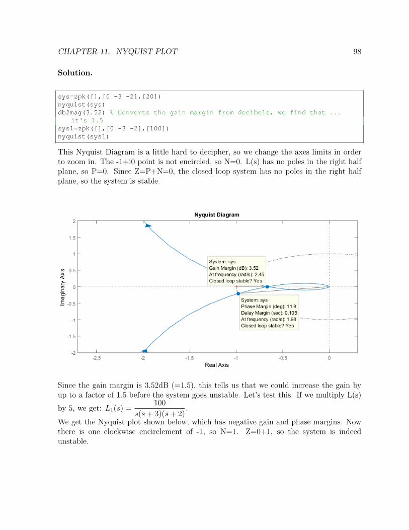
CHAPTER 11. NYQUIST PLOT 98
Solution.
sys=zpk([],[0 -3 -2],[20])nyquist(sys)db2mag(3.52) % Converts the gain margin from decibels, we find that ...
it's 1.5sys1=zpk([],[0 -3 -2],[100])nyquist(sys1)
This Nyquist Diagram is a little hard to decipher, so we change the axes limits in orderto zoom in. The -1+i0 point is not encircled, so N=0. L(s) has no poles in the right halfplane, so P=0. Since Z=P+N=0, the closed loop system has no poles in the right halfplane, so the system is stable.
Since the gain margin is 3.52dB (=1.5), this tells us that we could increase the gain byup to a factor of 1.5 before the system goes unstable. Let’s test this. If we multiply L(s)
by 5, we get: L1(s) =100
s(s+ 3)(s+ 2).
We get the Nyquist plot shown below, which has negative gain and phase margins. Nowthere is one clockwise encirclement of -1, so N=1. Z=0+1, so the system is indeedunstable.

CHAPTER 11. NYQUIST PLOT 99
We can verify the result by checking the root locus diagram:
Example 11.3.2. Find the range of K for stability of the following unit-feedback system:
G(s) =K
s− 5.
Solution.
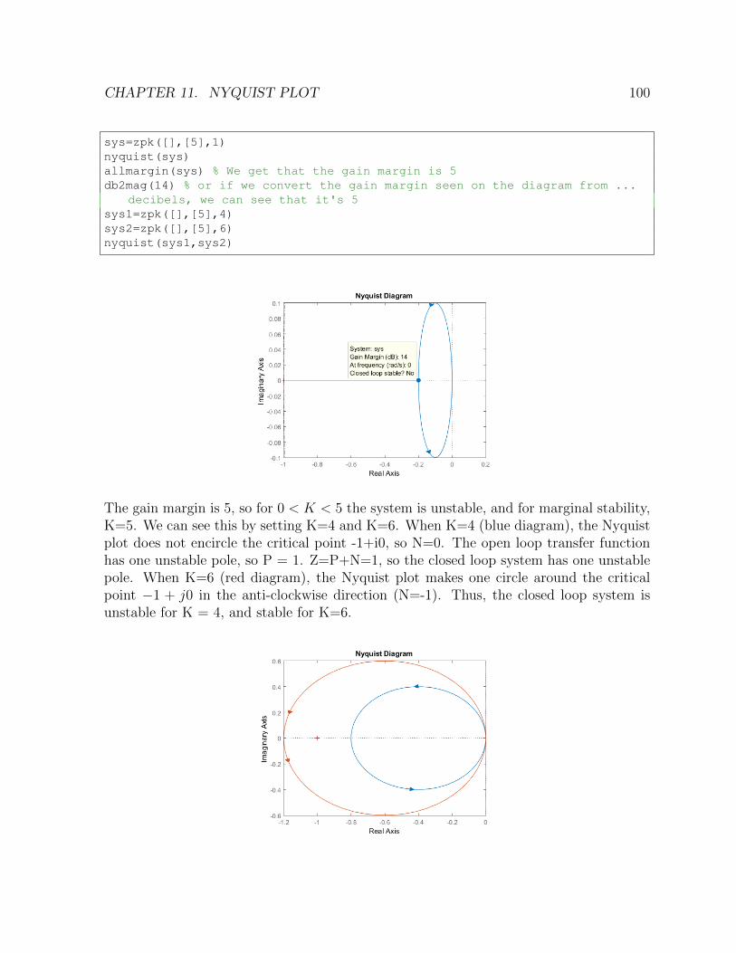
CHAPTER 11. NYQUIST PLOT 100
sys=zpk([],[5],1)nyquist(sys)allmargin(sys) % We get that the gain margin is 5db2mag(14) % or if we convert the gain margin seen on the diagram from ...
decibels, we can see that it's 5sys1=zpk([],[5],4)sys2=zpk([],[5],6)nyquist(sys1,sys2)
The gain margin is 5, so for 0 < K < 5 the system is unstable, and for marginal stability,K=5. We can see this by setting K=4 and K=6. When K=4 (blue diagram), the Nyquistplot does not encircle the critical point -1+i0, so N=0. The open loop transfer functionhas one unstable pole, so P = 1. Z=P+N=1, so the closed loop system has one unstablepole. When K=6 (red diagram), the Nyquist plot makes one circle around the criticalpoint −1 + j0 in the anti-clockwise direction (N=-1). Thus, the closed loop system isunstable for K = 4, and stable for K=6.

CHAPTER 11. NYQUIST PLOT 101
Example 11.3.3. [Nise, 2013, Thomas et al., 2005] A room’s temperature can be con-trolled by varying the radiator power. In a specific room, the transfer function fromindoor radiator power, Q, to room temperature, T in , is
P (s) =T (s)
Q(s)=
(1× 10⁻⁶)s2 + (1.314× 10⁻⁹)s+ (2.66× 10⁻¹³)
s3 + 0.00163s2 + (5.272× 10⁻⁷)s+ (3.538× 10⁻¹¹)
The system is controlled in a negative feedback closed-loop configuration with G(s)=KP(s).a. Draw the corresponding Nyquist diagram for K=1.b. Obtain the gain and phase margins.c. Find the range of K for the closed-loop stability.
Solution.
sys=tf([1*10ˆ(-6) 1.314*10ˆ(-9) 2.66*10ˆ(-13)],[1 0.00163 5.272*10ˆ(-7) ...3.538*10ˆ(-11)])
nyquist(sys)% Plots the Nyquist diagram
The gain margin is infinite as the plot never crosses the 180o
line. The phase margin isundefined since |G(jw)| < 1 at all frequencies, and the system is closed loop stable for all0 < K <∞.
Example 11.3.4. [Nise, 2013, Kim et al., 2009] An experimental holographic media stor-age system uses a flexible photopolymer disk. During rotation, the disk tilts, making in-formation retrieval difficult. A system that compensates for the tilt has been developed.For this, a laser beam is focused on the disk surface and disk variations are measured

CHAPTER 11. NYQUIST PLOT 102
through reflection. A mirror is in turn adjusted to align with the disk and makes infor-mation retrieval possible. The system can be represented by a unity feedback system inwhich a controller with transfer function:
GC(s) =78.575(s+ 436)2
(s+ 132)(s+ 8030)
and a plant
P (s) =1.163× 10⁸
s3 + 962.5s2 + 5.958× 10⁵s+ 1.16× 10⁸
from an open loop transmission L(s) = GC(s)P (s).a. Use MATLAB to obtain the system’s Nyquist diagram. Find out if the system isstable.b. Find the system’s phase and gain margin.
Solution.
s=tf('s');P=1.163e8/(sˆ3+962.5*sˆ2+5.958e5*s+1.16e8);G=78.575*(s+436)ˆ2/(s+132)/(s+8030);L=G*P;nyquist(L)
The system is closed-loop stable and it can be seen from the plot that the phase marginis 10.5 degrees. Also the gain margin is 6.06dB.
Example 11.3.5. [Nise, 2013] Find the range of K for stability, for each of the followingsystems that are controlled in a feedback closed-loop configuration with:
1. G(s) =K
(s+ 2)and feedback gain H(s) =
1
(s+ 4)(s+ 6).

CHAPTER 11. NYQUIST PLOT 103
2. G(s) =K(s2 − 4s+ 13)
(s+ 2)(s+ 4), and feedback gain H(s) =
1
s.
Solution.
sys1=zpk([],[-2 -4 -6],1)nyquist(sys1)db2mag(53.6) % Converts the gain margin from decibels, we find that ...
it's 478.63
The Nyquist diagram intersects the real axis at -0.0021. The open-loop transfer functionhas no unstable poles, so P=0. Hence, Z=P+N, Z=0+0 if K < 478.63, and Z=0+2 ifK > 478.63. Therefore, we have stability if 0 < K < 478.63.b.
p=tf([1 -4 13],[1 0]);q=zpk([],[-2 -4],1);sys=p*qnyquist(sys)db2mag(2.85) % Converts the gain margin from decibels, we can see that ...
it's 1.39

CHAPTER 11. NYQUIST PLOT 104
The Nyquist diagram intersects the real axis at -0.72 and P = 0. Hence, Z = P + N,Z=0+0 if K < 1.39, and Z=0+2 if K > 1.39. Therefore, stability if 0 < K < 1.39.
Example 11.3.6. Find the range of K for stability of the following unit-feedback system:
K
(s− 0.5)(s+ 3)(s+ 6)
Solution.
sys=zpk([],[0.5 -3 -6],1)nyquist(sys)allmargin(sys) % The gain margin is the interval [9 123.7198]

CHAPTER 11. NYQUIST PLOT 105
The gain margin here is an interval, because as we can see from the root locus plot, thesystem from unstable becomes stable at gain 9, and then it becomes unstable again.
Chapter 12
Control Systems Toolbox
12.1 Introduction
In this chapter a useful Matlab® application called the Control Systems Toolbox® willbe presented. This Toolbox allows us to define complicated systems (as in Simulink®)and by interactively modifying the systems parameters, observe the changes made in thesystem’s response, root locus, Nyquist and Bode diagrams.
So when using this Toolbox, we can input our desired plant, either in a transferfunction or a state space form, choose the systems structure from a predefined set ofavailable options and observe the systems behavior in the time (step/ramp responses,root locus) or frequency (Nyquist and Bode plots) domain. These functionalities will beexplicitly presented in the following sections.
12.2 Designing the system
First of all, in order to open up the Control Systems Toolbox®, type sisotool in thecommand window. Alternatively, you can find the Toolbox from Matlab’s® APPS tab.
A window will pop up looking like this: 1
1An additional window with blank plots may appear too. Ignore this for now.
106

CHAPTER 12. CONTROL SYSTEMS TOOLBOX 107
This is the main interface of the Toolbox. It contains five tabs, namely Architecture,Compensator Editor, Graphical Tuning, Analysis Plots and Automated Tuning. We willfocus on the main aspects of each tab.
On Architecture, one can choose the basic structure of the system and import itsplant. On Control Architecture one can choose between six different system structures.On System Data, one can choose the values of each block F, C, G, H. It is here that wecan import the plant for the system. By clicking on this option, a new window pops up

CHAPTER 12. CONTROL SYSTEMS TOOLBOX 108
Here we can import the desired plant that we should have previously defined in ourworkspace. So here it should be understandable that there exists a system variable calledsys in the workspace. One can also directly input numerical values for the blocks, but itis preferable to do so from the Compensator tab.
On Compensator Editor, one can edit the compensator blocks of the system. Youcan change the gain value and add or remove poles and zeros by right clicking on theblank space above Pole/Zero. The values of these parameters though can also changeinteractively by “moving along”the root locus, as we shall see later.
On Graphical Tuning, one can choose among three different plots: Root locus, openloop Bode plot, and Nichols plot. Once the plots have been chosen, a new window willpop up displaying the user’s choices. Root locus and Bode are the most usual tools insystem analysis.
Here lies the strongest advantage of the Control Systems Toolbox®, which we willexplain in the following examples. This is the fact that we can interactively change thevalue of the compensator gain C by placing the poles on the desired positions in the rootlocus, or by dragging the magnitude curve of the Bode plot up or down. In addition tothis, one can input design constraints in these plots, which help in the system design.
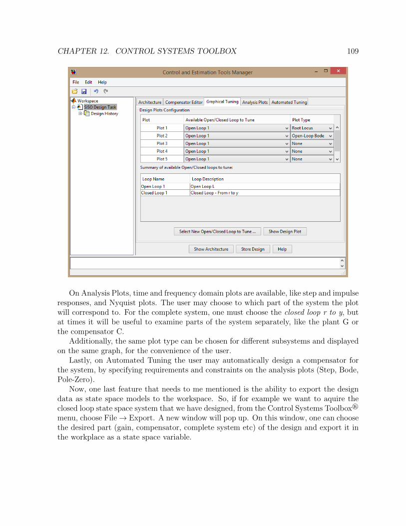
CHAPTER 12. CONTROL SYSTEMS TOOLBOX 109
On Analysis Plots, time and frequency domain plots are available, like step and impulseresponses, and Nyquist plots. The user may choose to which part of the system the plotwill correspond to. For the complete system, one must choose the closed loop r to y, butat times it will be useful to examine parts of the system separately, like the plant G orthe compensator C.
Additionally, the same plot type can be chosen for different subsystems and displayedon the same graph, for the convenience of the user.
Lastly, on Automated Tuning the user may automatically design a compensator forthe system, by specifying requirements and constraints on the analysis plots (Step, Bode,Pole-Zero).
Now, one last feature that needs to me mentioned is the ability to export the designdata as state space models to the workspace. So, if for example we want to aquire theclosed loop state space system that we have designed, from the Control Systems Toolbox®
menu, choose File→ Export. A new window will pop up. On this window, one can choosethe desired part (gain, compensator, complete system etc) of the design and export it inthe workplace as a state space variable.
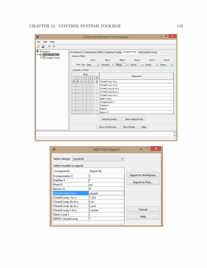
CHAPTER 12. CONTROL SYSTEMS TOOLBOX 110

CHAPTER 12. CONTROL SYSTEMS TOOLBOX 111
12.3 Examples
Example 12.3.1. Consider the following system
After you import this system in sisotool:
1. Plot system’s step response for K=2.
2. Plot the system’s root locus.
3. Find the closed loop transfer function.

CHAPTER 12. CONTROL SYSTEMS TOOLBOX 112
Solution. First, we begin by defining the different blocks in Matlab. Then we open upsisotool and import these blocks to the system
sys fw=tf(10, [1 1 10]); % The open loop blocksys bw=tf(1,[1 2]); % The feedback blocksisotool %opens sisotool
After we import the above transfer function blocks in SISOtool, we choose the correctvalue for K from Compensator Editor, and also add an additional zero at 0. The rootlocus and step response of the system are the following
Now, in order to find the closed loop transfer function, we export the closed loop r toy system , and using the transfer function command, we get
Closed(s) =20s+ 40
s4 + 3s3 + 12s2 + 20s+ 20
Example 12.3.2. Consider the closed loop system with open loop transfer function
G(s) =K
(s+ 1)(s+ 2)
After you import this system in sisotool:
1. Using the root locus, find the gain matrix K such that the system has an Overshootof 4%.
2. Plot the system’s step response.
3. Find the closed loop transfer function.

CHAPTER 12. CONTROL SYSTEMS TOOLBOX 113
Solution. First, we begin by defining the transfer function in the command window.Then, after we import the above transfer function in SISOtool, we open up the root locusplot and input the desired constraints. Then, we interactively change the gain in orderto place the system’s poles on the intersections of the root locus and the constraint lines,just like the following image shows.
Now, in order to find the closed loop transfer function, we export the closed loop r toy system , and using the transfer function command, we get
Closed(s) =2.335
s2 + 3s+ 4.335
Example 12.3.3. [Nise, 2013, Yan and Lin, 2003] The read/write head assembly arm ofa computer hard disk drive (HDD) can be modeled as a rigid rotating body with inertiaIb. Its dynamics can be described with the transfer function
P (s) =X(s)
F (s)=
1
Ibs2
where X(s) is the displacement of the read/write head and F(s) is the applied force (Yan,2003). Assume the arm has an inertia of 3 · 10−5kg ·m2 and that a lead controller Gc isplaced in series to yield the following system
with open loop transfer function
G(s) = Gc(s)P (s) =K
Ibs2
(s+ 1)
(s+ 10)
After you import this system in sisotool:

CHAPTER 12. CONTROL SYSTEMS TOOLBOX 114
1. Find the value of K that will result in dominant complex conjugate poles with aζ = 0.707 damping factor.
2. Plot the system’s impulse and step responses.
Solution. First, we begin by defining the different blocks in Matlab. Then we open upsisotool and import these blocks to the system. The next step is to import the desiredconstraint of ζ = 0.707 on the root locus. Then, we interactively change the gain in orderto place the system’s poles on the intersections of the root locus and the constraint lines,just like the following image shows
This corresponds to a gain value of K = 6.8138 · 10−6 and closed loop poles s =−7.6866, −1.1567 ± 1.1495i. It is clear that we have two complex conjugate poles thatconstitute the dominant poles of the system and one more real pole that is far on the leftand thus much less important in the dynamic behavior of the closed loop system.
The step and impulse responses are the following

CHAPTER 12. CONTROL SYSTEMS TOOLBOX 115
Chapter 13
Designing Controllers Using theControl Systems Toolbox
13.1 Introduction
Using SISOtool, one can interactively design controllers for the system, in order to changeits characteristics. The observer design can have two different aims. Either change thetransient response characteristics of the system (rise time, settling time, % overshoot)or change its steady state characteristics (steady state). Of course, more advanced con-trollers, like PID controllers, can change both transient and steady state characteristicsof a system.
The basic idea behind controller design is this. Change the root locus of the system,in order to make it pass through specific points that satisfy the design requirements. Howcan this be achieved though?
As is well known, for any point s0 in the root locus, the angular contribution of thepoles and zeros of the system satisfies
∠G(s)|s=s0 = (2k + 1)π
So the main idea of the design is to add poles and zeros to the system, so that the angularcontribution at the desired points in the Complex Plane satisfies the above relation.
13.2 Improving Transient Response
To improve the transient response of the system, PD and Lead compensators are used.Their characteristics are shown in the following table
116

CHAPTER 13. DESIGNING CONTROLLERS USING THE CONTROL SYSTEMS TOOLBOX117
Ideal ProportionalDerivative (PD)
C(s) = K(s+ zc) A gain plus a differentiator.
Lead C(s) = K s+as+r·a , 1 ≤ r ≤ 10 The pole is further on the left, so
that the angular contribution ispositive ∠(s+a)−∠(s+r ·a) > 0.
Lead compensators are actually an approximation of a PD. The change these com-pensators bring about on the root locus will be made clear in the following examples.
13.2.1 Examples
Example 13.2.1. [Dorf and Bishop, 2009] Designers have developed small, fast, vertical-takeoff fighter aircraft that are invisible to radar (stealth aircraft). This aircraft conceptuses quickly turning jet nozzles to steer the airplane [22]. The control system for the head-ing or direction control is a unity feedback system with the Aircraft dynamics describedby the transfer function
Gplant =s+ 20
s(s+ 10)2(13.1)
along with a Proportional Controller. Plot the root locus and determine the maximumgain K that ensures stability.
Solution. If we plot the root locus of the above system, we can see that the locus liescompletely on the negative part of the complex plane. That means that the system isstable for all K > 0. So the usage of the Proportional gain K lies in the tuning of theresponse characteristics of the system.

CHAPTER 13. DESIGNING CONTROLLERS USING THE CONTROL SYSTEMS TOOLBOX118
Example 13.2.2. [Nise, 2013, Yan and Lin, 2003] Going back to Example 12.3.3, wehave the read/write head assembly arm of a computer hard disk drive (HDD), whosedynamics are described by the open loop transfer function
P (s) =X(s)
F (s)=
3 · 105
s2
To this system we add a lead controller in order to change the systems stability. Ouraim is to find a lead or PD controller such that for an appropriate gain value K the systemhas dominant conjugate poles with a ζ = 0.707 damping factor.
Solution. Let us consider the compensator
Gc(s) = Ks+ 1
s+ r · 1(13.2)
After we import the system in sisotool, we try different values for r, moving the poleof the system further to the left in the complex plane little by little. This can be doneeither in the compensator editor or by moving the pole of the compensator in the rootlocus (the red “x”). This change in the root locus is displayed in the following figures
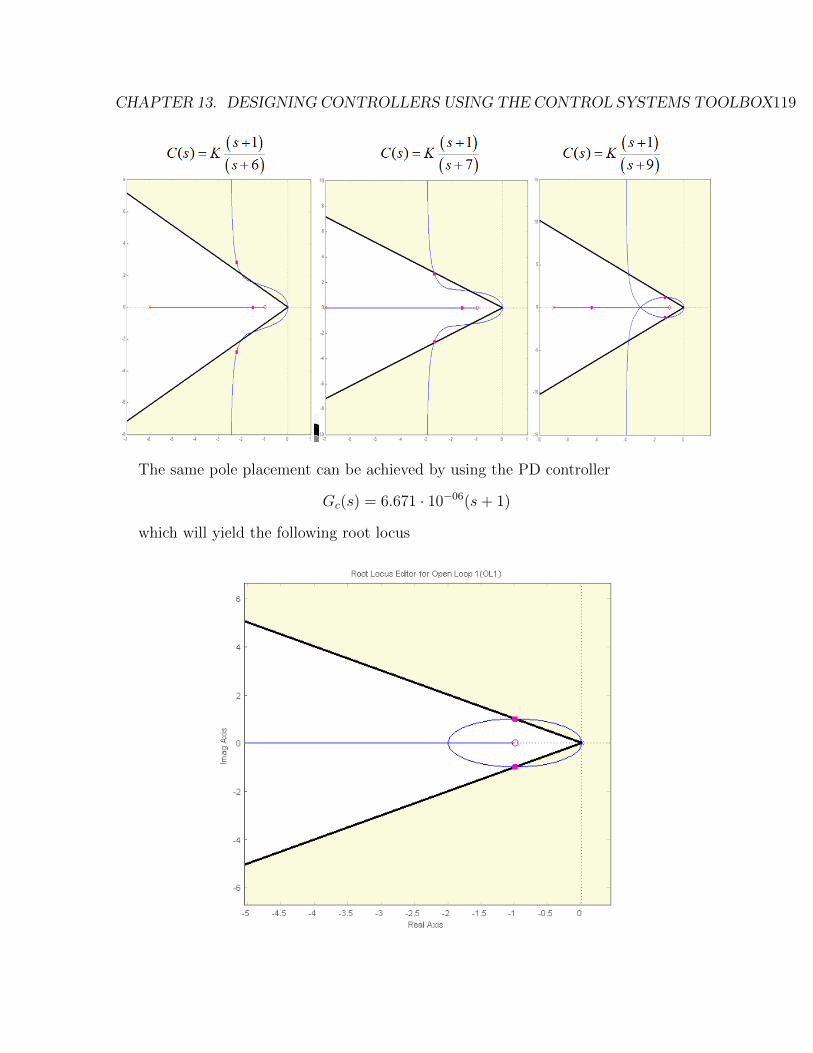
CHAPTER 13. DESIGNING CONTROLLERS USING THE CONTROL SYSTEMS TOOLBOX119
The same pole placement can be achieved by using the PD controller
Gc(s) = 6.671 · 10−06(s+ 1)
which will yield the following root locus

CHAPTER 13. DESIGNING CONTROLLERS USING THE CONTROL SYSTEMS TOOLBOX120
Example 13.2.3. [Dorf and Bishop, 2009, de Panne et al., 1992] Automatic control sys-tems are used to aid and control the walk of partially disabled persons. One model of asystem that is open-loop unstable is shown in the following figure
1. Using the root locus in SISOtool, find the value of K that achieves the maximumnumber of damping factor ζ.
2. Plot the step response of the system.
Solution. Importing the system in sisotool, we plot the root locos of the system. We cansee that the addition of the lead compensator can drive the system to stability for gainvalues K > 2.6.
Now, the maximum damping factor for complex roots is achieved for the smaller anglethe root locus makes with the real axis, as is seen in the following figure

CHAPTER 13. DESIGNING CONTROLLERS USING THE CONTROL SYSTEMS TOOLBOX121
This point corresponds to a damping factor ζ = 0.446 and the compensator is
Gc(s) =65.968(s+ 2)
(s+ 10)
the step response for the system is the following
Example 13.2.4. [Dorf and Bishop, 2009, Martin, 1999] A unity feedback control systemfor a robot submarine has a plant with a third-order transfer function
G(s) = K1
s(s+ 10)(s+ 50)
Add a lead controller to this system, in order to achieve an overshoot of approximately7.5% and a settling time of 0.4sec. Let the zero of the controller be located at -15.
Solution. Let us consider the lead controller
Gc(s) = Ks+ 15
s+ r · 15(13.3)
This means that since we have created a lead controller, the pole must be further on theleft than the zero on the complex plane. Importing the system and design requirementsin sisotool we get the following root locus (before we add the controller)

CHAPTER 13. DESIGNING CONTROLLERS USING THE CONTROL SYSTEMS TOOLBOX122
So the system obviously does not satisfy the design requirements. Now, adding the con-troller and trying different values for its pole, we end up with
Gc(s) = 63493s+ 15
s+ 130(13.4)
which gives us the following root locus and step response
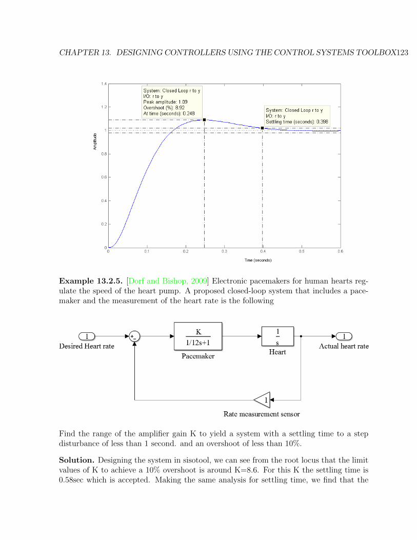
CHAPTER 13. DESIGNING CONTROLLERS USING THE CONTROL SYSTEMS TOOLBOX123
Example 13.2.5. [Dorf and Bishop, 2009] Electronic pacemakers for human hearts reg-ulate the speed of the heart pump. A proposed closed-loop system that includes a pace-maker and the measurement of the heart rate is the following
Find the range of the amplifier gain K to yield a system with a settling time to a stepdisturbance of less than 1 second. and an overshoot of less than 10%.
Solution. Designing the system in sisotool, we can see from the root locus that the limitvalues of K to achieve a 10% overshoot is around K=8.6. For this K the settling time is0.58sec which is accepted. Making the same analysis for settling time, we find that the
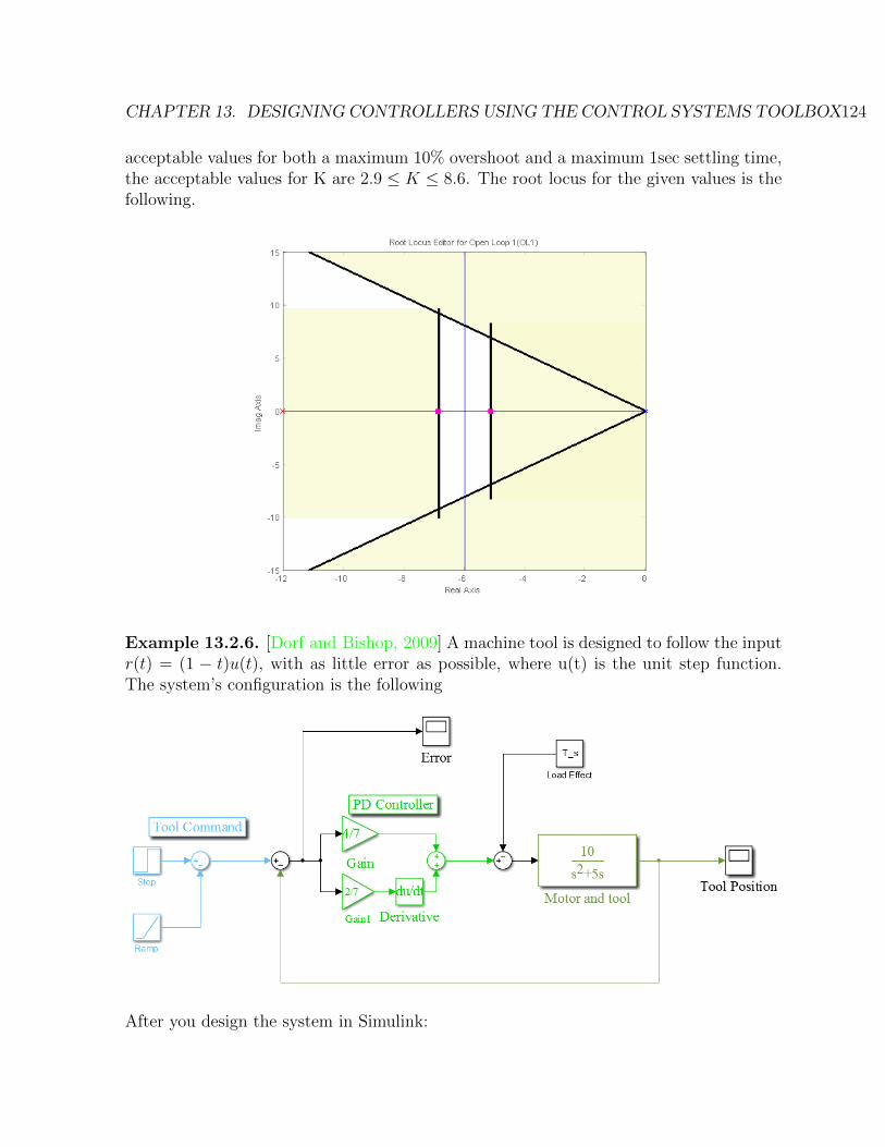
CHAPTER 13. DESIGNING CONTROLLERS USING THE CONTROL SYSTEMS TOOLBOX124
acceptable values for both a maximum 10% overshoot and a maximum 1sec settling time,the acceptable values for K are 2.9 ≤ K ≤ 8.6. The root locus for the given values is thefollowing.
Example 13.2.6. [Dorf and Bishop, 2009] A machine tool is designed to follow the inputr(t) = (1 − t)u(t), with as little error as possible, where u(t) is the unit step function.The system’s configuration is the following
After you design the system in Simulink:

CHAPTER 13. DESIGNING CONTROLLERS USING THE CONTROL SYSTEMS TOOLBOX125
1. Plot the error between real and desired position for the given input, when the Loadeffect is zero, for 0 ≤ t ≤ 10.
2. Plot the error between real and desired position when the input is zero and the Loadeffect is Td(s) = 1
s.
Solution. We begin by designing the system in Simulink and tuning all the systemsparameters, such as the simulation time for the model and the step time in the stepblock. For a load effect equal to zero, we get the following error and response plots
Now, if we assume a zero input and a load effect equal to a step signal, we get the followingresults

CHAPTER 13. DESIGNING CONTROLLERS USING THE CONTROL SYSTEMS TOOLBOX126
13.3 Improving Steady State Response
To improve the steady state response of the system, PI and Lag compensators are used.Their characteristics are shown in the following table
Ideal Proportional In-tegral (PI)
C(s) = K s+as
Pure integrator that increases thesystem type and drives the errorto zero.
Lag C(s) = K s+r·as+a
, 1 ≤ r ≤ 10 Approximates an integrator andreduces the error.
The idea behind an Integral compensator is to increase the system Type. By that, wemean the number of system’s poles located at 0. So in general, if we consider systems ofthe form
G(s) =(s+ z1)(s+ z2) · · ·sn(s+ p1)(s+ p2) · · ·
(13.5)
for n = 0, the system is of Type 0, for n = 1 of Type 1 etc. The system Type is crucial indefining the steady state error of the system to different kind of responses. For example,a Type 1 system will have zero steady state error to step input, constant error to rampinput and an infinite error to parabola input.
The zero a is always placed near zero, so that the angular contribution of the controlleris approximately equal to zero. Thus the root locus remains unchanged.
Lag compensators are actually an approximation of a PI. The change these compen-sators bring about on the root locus will be made clear in the following examples.
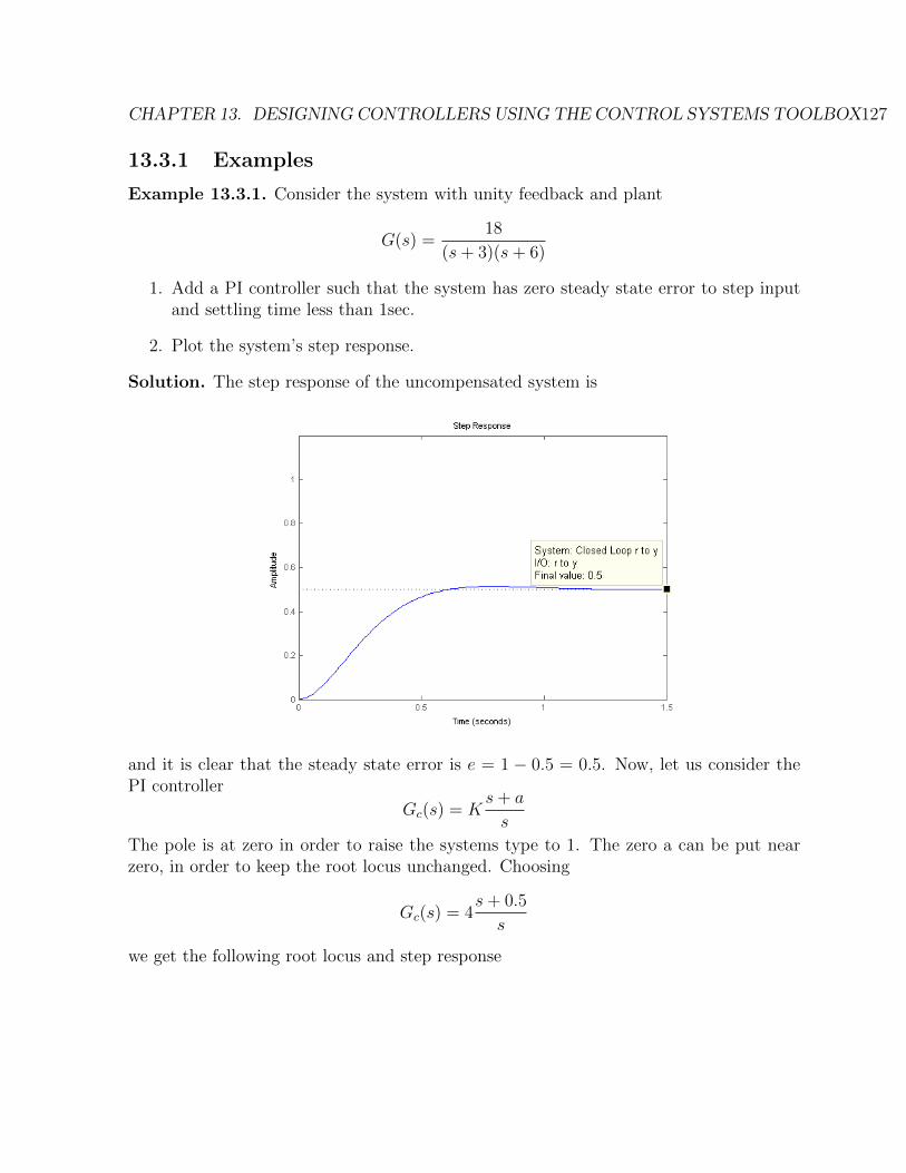
CHAPTER 13. DESIGNING CONTROLLERS USING THE CONTROL SYSTEMS TOOLBOX127
13.3.1 Examples
Example 13.3.1. Consider the system with unity feedback and plant
G(s) =18
(s+ 3)(s+ 6)
1. Add a PI controller such that the system has zero steady state error to step inputand settling time less than 1sec.
2. Plot the system’s step response.
Solution. The step response of the uncompensated system is
and it is clear that the steady state error is e = 1 − 0.5 = 0.5. Now, let us consider thePI controller
Gc(s) = Ks+ a
s
The pole is at zero in order to raise the systems type to 1. The zero a can be put nearzero, in order to keep the root locus unchanged. Choosing
Gc(s) = 4s+ 0.5
s
we get the following root locus and step response

CHAPTER 13. DESIGNING CONTROLLERS USING THE CONTROL SYSTEMS TOOLBOX128
which makes it clear that the error is equal to zero.
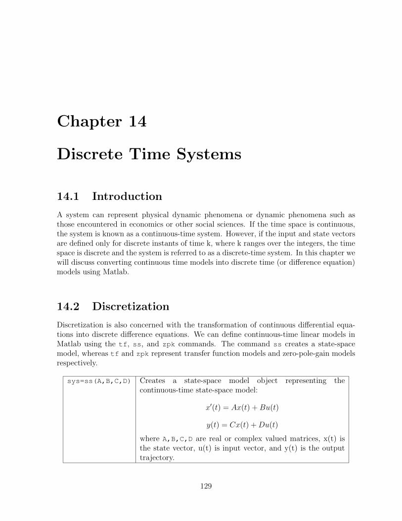
Chapter 14
Discrete Time Systems
14.1 Introduction
A system can represent physical dynamic phenomena or dynamic phenomena such asthose encountered in economics or other social sciences. If the time space is continuous,the system is known as a continuous-time system. However, if the input and state vectorsare defined only for discrete instants of time k, where k ranges over the integers, the timespace is discrete and the system is referred to as a discrete-time system. In this chapter wewill discuss converting continuous time models into discrete time (or difference equation)models using Matlab.
14.2 Discretization
Discretization is also concerned with the transformation of continuous differential equa-tions into discrete difference equations. We can define continuous-time linear models inMatlab using the tf, ss, and zpk commands. The command ss creates a state-spacemodel, whereas tf and zpk represent transfer function models and zero-pole-gain modelsrespectively.
sys=ss(A,B,C,D) Creates a state-space model object representing thecontinuous-time state-space model:
x′(t) = Ax(t) +Bu(t)
y(t) = Cx(t) +Du(t)
where A,B,C,D are real or complex valued matrices, x(t) isthe state vector, u(t) is input vector, and y(t) is the outputtrajectory.
129

CHAPTER 14. DISCRETE TIME SYSTEMS 130
The syntax for creating discrete-time models is similar to that for continuous-time models,except that we must also provide a sample time (sampling interval in seconds).
sys=ss(A,B,C,D,Ts) Creates the discrete-time state-space model:
x[n+ 1] = Ax[n] +Bu[n]
y[n] = Cx[n] +Du[n]
with sample time Ts (in seconds)sys=tf(num,den,Ts) Creates a discrete-time transfer function with sample time
Ts (in seconds). The input arguments num and den are asin the continuous-time case and must list the numerator anddenominator coefficients in descending powers of z.
sys=zpk(z,p,k,Ts) Creates a discrete-time zero-pole-gain model with sample timeTs (in seconds). The input arguments z,p,k are as in thecontinuous-time case.
For example, to specify the discrete-time transfer function: H(z) =z − 1
z2 − 1.85z + 0.9with
sampling period Ts = 0.2s, we type the following:
num=[1 -1];den=[1 -1.85 0.9];H=tf(num,den,0.2)
To specify the discrete-time state-space model:
x[k + 1] = 0.5x[k] + u[k]
y[k] = 0.2x[k],
with sampling period Ts = 0.1s, we type:
sys = ss(.5,1,.2,0,0.1)
In Matlab, the c2d command discretizes continuous-time models. Conversely, d2cconverts discrete-time models to continuous time. Commands c2d and d2c support thefollowing discretization and interpolation methods:• Zero-Order Hold (zoh): The Zero-Order Hold method provides an exact match betweenthe continuous and discrete-time systems in the time domain for staircase inputs. Thefollowing block diagram shows the zero-order-hold discretization Hd(z) of a continuous-time linear model H(s).
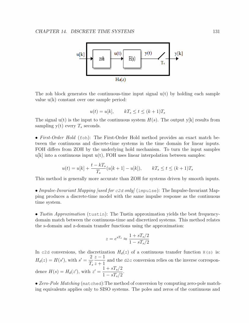
CHAPTER 14. DISCRETE TIME SYSTEMS 131
The zoh block generates the continuous-time input signal u(t) by holding each samplevalue u(k) constant over one sample period:
u(t) = u[k], kTs ≤ t ≤ (k + 1)Ts
The signal u(t) is the input to the continuous system H(s). The output y[k] results fromsampling y(t) every Ts seconds.
• First-Order Hold (foh): The First-Order Hold method provides an exact match be-tween the continuous and discrete-time systems in the time domain for linear inputs.FOH differs from ZOH by the underlying hold mechanism. To turn the input samplesu[k] into a continuous input u(t), FOH uses linear interpolation between samples:
u(t) = u[k] +t− kTsTs
(u[k + 1]− u[k]), kTs ≤ t ≤ (k + 1)Ts
This method is generally more accurate than ZOH for systems driven by smooth inputs.
• Impulse-Invariant Mapping [used for c2d only] (impulse): The Impulse-Invariant Map-ping produces a discrete-time model with the same impulse response as the continuoustime system.
• Tustin Approximation (tustin): The Tustin approximation yields the best frequency-domain match between the continuous-time and discretized systems. This method relatesthe s-domain and z-domain transfer functions using the approximation:
z = esTs ≈ 1 + sTs/2
1− sTs/2
In c2d conversions, the discretization Hd(z) of a continuous transfer function H(s) is:
Hd(z) = H(s′), with s′ =2
Ts
z − 1
z + 1and the d2c conversion relies on the inverse correspon-
dence H(s) = Hd(z′), with z′ =
1 + sTs/2
1− sTs/2.
• Zero-Pole Matching (matched):The method of conversion by computing zero-pole match-ing equivalents applies only to SISO systems. The poles and zeros of the continuous and

CHAPTER 14. DISCRETE TIME SYSTEMS 132
discretized systems are related by the transformation: zi = esiTs , where zi is the ith poleor zero of the discrete-time system, si is the ith pole or zero of the continuous-time systemand Ts is the sample time.
c2d(sys,Ts,method) Discretizes the continuous-time dynamic sys-tem model sys using the specified discretizationmethod method. We write: c2d(sys,Ts,'zoh'),c2d(sys,Ts,'foh'), c2d(sys,Ts,'impulse'),c2d(sys,Ts,'tustin') orc2d(sys,Ts,'matched'), according to the methodthat we want to use.
d2c(sys,method) Produces a continuous-time model that is equiva-lent to the discrete-time dynamic system modelsys using the specified conversion methodmethod. We write: c2d(sys,Ts,'zoh'),c2d(sys,Ts,'foh'), c2d(sys,Ts,'tustin')
or c2d(sys,Ts,'matched'), according to themethod that we want to use.
sys1=d2d(sys,Ts) Resamples the discrete-time dynamic system modelsys to produce an equivalent discrete-time modelsys1 with the new sample time Ts (in seconds), usingzero-order hold on the inputs.
sys1=d2d(sys,Ts,method) Resamples the discrete-time dynamic system modelsys to produce an equivalent discrete-time modelsys1 with the new sample time Ts (in seconds), us-ing the specified resampling method method, whichcan be 'zoh' (Zero-order hold) or 'tustin' (Tustinapproximation).
14.3 Examples
Example 14.3.1. Discretize the following state-space system with zero-order hold andfirst-order hold:
x′(t) =
(−0.5 2
0 −0.5
)x(t) +
(01
)u(t)
y(t) =(1 0
)x(t)
Solution.
A=[-0.5 2;0 -0.5];B=[0;1];C=[1 0];

CHAPTER 14. DISCRETE TIME SYSTEMS 133
D=0;sys=ss(A,B,C,D); % Creates the state-space modelsys d1=c2d(sys,1,'foh') % Discretizes sys using first-order holdsys d2=c2d(sys,1,'zoh') % Discretizes sys using zero-order hold
Example 14.3.2. [Kelley and Peterson, 2001] In a certain agricultural delta, populationsof owls and mice coexist under normal conditions in a predator and prey relationship, to astable equilibrium population of O thousand owls and M million mice. However, extremewinter conditions can reduce the owl population drastically. In the model below, the owland mouse populations are gradually restored to their normal equilibria.
Let x(k) and y(k) denote the deviations of the owl and mouse populations respectively,from their usual levels at the beginning of the k-th year, so that O+x(t) is the populationof owls (in thousands) and M+y(k) is the population of mice (in millions). Their relationis described by the following system of two difference equations(
x(k + 1)y(k + 1)
)=
(0.9 0.2−0.1 0.6
)(x(k)y(k)
)Define the following system as a discrete time state space system with a period of T=1
year and plot the two states for initial conditions x(0) = −5 and y(0) = 0 for a period of15 years.
Solution.
% First we define the discrete time systemsys=ss([0.9,0.2;-0.1,0.6],[0;0],eye(2),0,1);y=initial(sys,[-5,0],15);% The above vector y has two columns, one for each state of the systemyears=0:15;plot(years,y(:,1)','s')hold allplot(years,y(:,2)','s')legend('owl population deviation','mice population deviation')

CHAPTER 14. DISCRETE TIME SYSTEMS 134
From the figure we can observe that the deviations of the two populations tend to zeroafter a period of about 14 years.
Example 14.3.3. Consider a system with the following transfer function
G(s) =49
s2 + 2s+ 49
Discretize the following system, choosing a sampling period that accurately preserves itsdynamic characteristics.
Solution. We should choose a sampling frequency that is at least 2 times higher thanthe natural frequency of the system . Since ω = 7, a sampling time of
ωs = 3ω ⇒ 1/Ts = 3ω ⇒ Ts = 1/21 = 0.0476sec
will yield an accurate enough discrete time system.
sys=tf(49,[1 2 49])sysd=c2d(sys,0.0476)step(sys)hold allstep(sysd)legend('continuous system','discritized system')

CHAPTER 14. DISCRETE TIME SYSTEMS 135
Example 14.3.4. [Nise, 2013, Hardy, 1967] A six-degrees-of-freedom industrial robotequipped to perform arc welding and transfer objects according to a desired programcan be described by the following system:
1. If K=64510, define the system in Matlab using either the commands series, ...
feedback or Sisotool and find its transfer function.
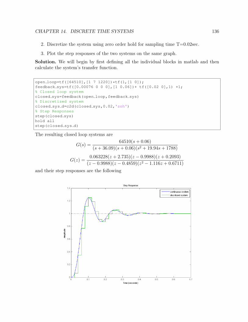
CHAPTER 14. DISCRETE TIME SYSTEMS 136
2. Discretize the system using zero order hold for sampling time T=0.02sec.
3. Plot the step responses of the two systems on the same graph.
Solution. We will begin by first defining all the individual blocks in matlab and thencalculate the system’s transfer function.
open loop=tf([64510],[1 7 1220])*tf(1,[1 0]);feedback sys=tf([0.00076 0 0 0],[1 0.06])+ tf([0.02 0],1) +1;% Closed loop systemclosed sys=feedback(open loop,feedback sys)% Discretized systemclosed sys d=c2d(closed sys,0.02,'zoh')% Step Responsesstep(closed sys)hold allstep(closed sys d)
The resulting closed loop systems are
G(s) =64510(s+ 0.06)
(s+ 36.09)(s+ 0.06)(s2 + 19.94s+ 1788)
G(z) =0.063228(z + 2.735)(z − 0.9988)(z + 0.2093)
(z − 0.9988)(z − 0.4859)(z2 − 1.116z + 0.6711)
and their step responses are the following
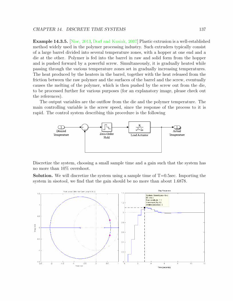
CHAPTER 14. DISCRETE TIME SYSTEMS 137
Example 14.3.5. [Nise, 2013, Dorf and Kusiak, 2007] Plastic extrusion is a well-establishedmethod widely used in the polymer processing industry. Such extruders typically consistof a large barrel divided into several temperature zones, with a hopper at one end and adie at the other. Polymer is fed into the barrel in raw and solid form from the hopperand is pushed forward by a powerful screw. Simultaneously, it is gradually heated whilepassing through the various temperature zones set in gradually increasing temperatures.The heat produced by the heaters in the barrel, together with the heat released from thefriction between the raw polymer and the surfaces of the barrel and the screw, eventuallycauses the melting of the polymer, which is then pushed by the screw out from the die,to be processed further for various purposes (for an explanatory image, please check outthe references).
The output variables are the outflow from the die and the polymer temperature. Themain controlling variable is the screw speed, since the response of the process to it israpid. The control system describing this procedure is the following
Discretize the system, choosing a small sample time and a gain such that the system hasno more than 10% overshoot.
Solution. We will discretize the system using a sample time of T=0.5sec. Importing thesystem in sisotool, we find that the gain should be no more than about 1.6878.
Chapter 15
Nonlinear Systems
15.1 Introduction
In this chapter examples of nonlinear systems will be presented. In linear systems, itis always possible to find the explicit solution using analysis methods. This is not thecase for nonlinear systems, where the computation of the solution can usually be achievedonly using numerical analysis methods. Additionally, new questions arise regarding theexistence of solution for given initial conditions.
Another notable feature of nonlinear systems is the high sensitivity to distrurbancesin the initial conditions. A small change in the initial condition of such a system (i.e. dueto rounding error) can yield a completely different response. This fact makes the longterm prediction of real life nonlinear phenomena an extremely tedious task.
An extensive analysis of nonlinear system theory can be found in [Hirsch et al., 2013]and [Khalil, 2002]. Here, we shall solve examples of nonlinear systems using Matlab andSimulink and present the dynamic behavior of their responses.
15.2 Examples
Example 15.2.1 (The Zaslavsky Map). The Zaslavsky Map [Zaslavsky, 1978] is a twodimensional discrete time dynamical system that exhibits chaotic behavior. It is describedby the following nonlinear equations
xn+1 =(xn + Ω
2π+ ( aΩ
2πΓ)(1− e−Γ)yn + K
Γ(1− e−Γ)cos(2πxn)
)mod1
yn+1 = e−Γ(yn + εcos(2πxn))
where K = aεΩ/2π, Ω, Γ, ε are the parameters of the system. Plot the points (xi, yi) ofthe system for the first 1500 terms of the sequence, for Ω = 100, ε = 0.3, Γ = 5, a = 1.885,K = 9.
Solution.
138

CHAPTER 15. NONLINEAR SYSTEMS 139
%% The Zaslavsky Map
%% Defining initial conditionsx(1)=0.1;y(1)=0.1;e=0.3;v=0.2;r=5;m=(1-exp(-r))/r;omega=100;k=9;a=1.885;
%% Computing the values for x(i),y(i)% We will compute the first 1500 values. They are more than enough to ...
get a clear view of the result.for i=2:1500
x(i)=mod(x(i-1)+omega/(2*pi)+(a*omega)/(2*pi*r)*(1-exp(-r))*y(i-1)+...(k/r)*(1-exp(-r))*cos(2*pi*x(i-1)),1);
% Since x(i) is computed mod1 we always have 0<=x(i)<1y(i)=exp(-r)*(y(i-1)+e*cos(2*pi*x(i-1)));
end
%% Plotting the resultsplot(x,y,'.','MarkerSize',1.4)axis([0 1 -0.003 0.003])
The map of the points (xi, yi) is the following

CHAPTER 15. NONLINEAR SYSTEMS 140
Example 15.2.2 (The Henon Map). The Henon Map [Henon, 1976] is a discrete timesystem that maps a point (xn, yn) using the following formula
xn+1 = 1− ax2n + yn
yn+1 = bxn(15.1)
Where a and b are the system parameters. Compute and plot the first 10000 points ofthis mapping for a=1.4 and b=0.3.
Solution.
%% We start by defining the initial valuesx(1)=0;y(1)=0;a=1.4;b=0.3;
%% Now we begin the iteration (10000 iterations):for i=2:10000
x(i)=1-1.4*(x(i-1)ˆ2)+y(i-1);y(i)=b*x(i-1);
endplot(x,y,'.','MarkerSize',4)title('Henon Map')
The plot of the above mapping is

CHAPTER 15. NONLINEAR SYSTEMS 141
Example 15.2.3 (The Lorenz Attractor). The Lorenz Attractor [Hirsch et al., 2013] isa famous nonlinear three dimensional system of differential equations that finds applica-tion in biology, circuit theory, mechanics, lasers and chemical reactions. The system isdescribed by the following differential equations
x′(t) =σ(y(t)− x(t)
)y′(t) =x(t)(ρ− z(t))− y(t)
z′(t) =βz(t) + x(t)y(t)
Where σ, ρ, β are the system parameters. Design the system in simulink and plot thepoints (xi, yi, zi) for σ = 10, ρ = 30, β = −3.
Solution. In order to solve the system, we choose here to design it first in Simulink andsave the simulation results in variables. For the parameter blocks σ, ρ, β we can choosedifferent values any time we run a simulation.
In order for the simulation results to be smooth, it is critical that we change the RefineFactor from Simulation Parameters of the model equal to 4. After the simulation is over(we can choose 70sec), we use the following commands to produce a rottating plot for thepoints (xi, yi, zi).
view(3)axis([-20,20,-30,30,0,50])f=plot3(x(1),y(1),z(1));

CHAPTER 15. NONLINEAR SYSTEMS 142
for i=2:length(tout)f=plot3(x(1:i),y(1:i),z(1:i));gridview(-37.5+i, 24)pause(0.01)
end
Example 15.2.4 (The Rossler Attractor). The Rossler Attractor [Rossler, 1976] is an-other three dimensional system of nonlinear differential equations
x′(t) =−y(t)− z(t)
y′(t) =x(t) + ay(t)
z′(t) =b+ z(t)(x(t)− c)
)Where a = 0.2, b = 0.2, c = 5.7 are the system parameters. Design this system in matlaband plot the points (xi, yi, zi).
Solution. Again changing the Refine Factor to 4 we design the nonlinear equations andsimulate the system for time T=300.

CHAPTER 15. NONLINEAR SYSTEMS 143
Again, we use the following commands to produce a rottating plot for (xi, yi, zi).
view(3)axis([-10,15,-15,10,-5,25])f=plot3(x(1),y(1),z(1));
for i=2:length(tout)f=plot3(x(1:i),y(1:i),z(1:i));gridview(-37.5+i, 24)pause(0.01)
end

CHAPTER 15. NONLINEAR SYSTEMS 144
Example 15.2.5 (Van der Pol Oscillator). The Van der Pol Oscillator [van der Pol, 1926]is a nonlinear equation that finds applications in various scientific fields like biology andseismology. It is described by the following differential equation
x′′(t)− µ(1− x(t)2)x′(t) + x(t) = 0 (15.2)
From the above equation it is clear that for µ = 0 the equation becomes linear. Simulatethe system for different values of µ and plot the values x(t), x′(t) against time, as well as(x(t), x′(t)).
Solution. Again changing the Refine Factor to 4 we design the nonlinear equations andsimulate the system for time T=200sec.

CHAPTER 15. NONLINEAR SYSTEMS 145
The functions x(t) and x′(t) for T = 50sec can be seen in the following figures
While the oscillation between these two functions for different values of µ can be seen inthe following figure

CHAPTER 15. NONLINEAR SYSTEMS 146
Acknowledgments
This book was typeset by the authors using LATEX, a free package of macro commandsbased on TEX, originally created by Leslie Lamport. The official page is http://www.
latex-project.org/
The authors would also like to acknowledge Florian Knorn for the creation of themcode package, which provided a handy way of visualizing Matlab code. It can be foundon Matlab Central.
Last but not least, many thanks goes to the online LATEX community of Stack-Exchangehttp://tex.stackexchange.com/ for being an encyclopaedia for LATEX debugging andproblem solving.
147

Bibliography
[Antsaklis and Michel, 2006] Antsaklis, P. J. and Michel, A. N. (2006). Linear systems.Boston: Birkhauser, 2nd corrected printing edition.
[Beucher and Weeks, 2008] Beucher, O. and Weeks, M. (2008). Introduction to MATLAB& SIMULINK: A Project Approach. Engineering series. Infinity Science Press.
[Brian Douglas, 2013] Brian Douglas (2013). Videos on the nyquist stability criterion.https://www.youtube.com/watch?v=sof3meN96MA. Accessed: 10-07-2015.
[Cavallo et al., 1992] Cavallo, A., Maria, G. D., and Verde, L. (1992). Robust flight con-trol systems - a parameter space design. Journal of Guidance, Control, and Dynamics,15(5):1207–1215.
[Chaturvedi, 2010] Chaturvedi, D. K. (2010). Modeling and simulation of systems usingMATLAB and Simulink. Boca Raton, FL: CRC Press.
[Cheever, 2005] Cheever, E. (2005). The nyquist plot online course. http://lpsa.
swarthmore.edu/Nyquist/Nyquist.html. Accessed: 10-07-2015.
[de Panne et al., 1992] de Panne, V., Fiume, and Vranesic (1992). A controller for thedynamic walk of a biped across variable terrain. In Proceedings of the 31st IEEEConference on Decision and Control, pages 2668–2673 vol.3.
[Digilent, 2010] Digilent (2010). Digital notes: Introduction to first order systemresponses. http://www.digilentinc.com/classroom/realanalog/text/Chapter_
2p4p1.pdf. Accessed: 10-07-2015.
[Dorf and Kusiak, 2007] Dorf, R. and Kusiak, A. (2007). Handbook of Design, Manufac-turing and Automation. John Wiley & Sons, Inc.
[Dorf and Bishop, 2009] Dorf, R. C. and Bishop, R. H. (2009). Modern control systems.Pearson Education, 11th edition.
[Elarafi and Hisham, 2008] Elarafi, M. and Hisham, S. (2008). Modeling and control ofpH neutralization using neural network predictive controller. In Control, Automationand Systems, 2008. ICCAS 2008. International Conference on, pages 1196–1199.
148
BIBLIOGRAPHY 149
[Fadali, 2015] Fadali, M. (2015). Root locus review. http://wolfweb.unr.edu/~fadali/ee472/RLocusRev.pdf. Accessed: 10-07-2015.
[Hardy, 1967] Hardy, H. (1967). Multi-Loop Servo Controls Programmed Robot. Instru-ments and Control Systems, page 105?111.
[Henon, 1976] Henon, M. (1976). A two-dimensional mapping with a strange attractor.Commun. Math. Phys., 50:69–76.
[Hespanha, 2009] Hespanha, J. P. (2009). Linear systems theory. Princeton, NJ: Prince-ton University Press.
[Hirsch et al., 2013] Hirsch, M. W., Smale, S., and Devaney, R. L. (2013). Differentialequations, dynamical systems, and an introduction to chaos. 3rd ed. Amsterdam: Aca-demic Press, 3rd ed. edition.
[Hong, 2015] Hong, X. (2015). Introduction to the nyquist criterion. http://www.
personal.reading.ac.uk/~sis01xh/teaching/CY2A9/Lecture7.pdf. Accessed: 10-07-2015.
[Houcque, 2005] Houcque, D. (2005). INTRODUCTION TO MATLAB FOR ENGI-NEERING STUDENTS, Northwestern University.
[Jiayu et al., 2009] Jiayu, K., Mengxiao, W., Linan, M., and Zhongjun, X. (2009). Cas-cade Control of the PH in an Anaerobic Wastewater Treatment System. In Bioinfor-matics and Biomedical Engineering , 2009. ICBBE 2009. 3rd International Conferenceon, pages 1–4.
[Kailath, 1980] Kailath, T. (1980). Linear Systems. Information and System SciencesSeries. Prentice-Hall.
[Kappos, 2002] Kappos, E. (2002). Classical Control Theory: A Course in the LinearMathematics of Systems and Control.
[Karris, 2011] Karris, S. (2011). Introduction to Simulink with Engineering Applications.Orchard Publications.
[Kelley and Peterson, 2001] Kelley, W. and Peterson, A. (2001). Difference equations. Anintroduction with applications. 2nd ed. San Diego, CA: Harcourt/Academic Press, 2nded. edition.
[Khalil, 2002] Khalil, H. K. (2002). Nonlinear systems. 3rd ed. Upper Saddle River, NJ:Prentice Hall, 3rd ed. edition.
[Kim et al., 2009] Kim, S., Kim, J., Yang, J., Yang, H., Park, J., and Park, Y. (2009).Tilt Detection and Servo Control Method for the Holographic Data Storage System.Microsyst Technol, 15:1695?1700.

BIBLIOGRAPHY 150
[Kuo et al., 2008] Kuo, C., Tsai, C., and Tu, H. (2008). Carriage speed control of across-lapper system for nonwoven web quality. Fibers and Polymers, 9(4):495–502.
[Liceaga-Castro and van der Molen, 1995] Liceaga-Castro, E. and van der Molen, G.(1995). Submarine H∞ depth control under wave disturbances. Control Systems Tech-nology, IEEE Transactions on, 3(3):338–346.
[Linkens, 1992] Linkens, D. (1992). Adaptive and intelligent control in anesthesia. ControlSystems, IEEE, 12(6):6–11.
[Liu et al., 2008] Liu, J.-H., ping Xu, D., and Yang, X.-Y. (2008). Multi-objective powercontrol of a variable speed wind turbine based H∞ on theory. In Machine Learning andCybernetics, 2008 International Conference on, volume 4, pages 2036–2041.
[M. Vajta, 2000] M. Vajta (2000). Some remarks on pade approximations. In Proceedingsof the 3rd TEMPUS-INTCOM Symposium, September 9-14, 2000, Veszpr?m, Hungary.Accessed: 10-07-2015.
[Magrab, 2011] Magrab, E. (2011). An Engineer’s Guide to MATLAB: With Applica-tions from Mechanical, Aerospace, Electrical, Civil, and Biological Systems Engineering.Pearson.
[Martin, 1999] Martin, F. (1999). The Art of Robotics. Prentice Hall.
[Mastascusa, 2015] Mastascusa, E. (2015). Online notes on nyquist plots, bucknell uni-versity course on electrical control systems. http://www.facstaff.bucknell.edu/
mastascu/econtrolhtml/Freq/Freq6.html. Accessed: 10-07-2015.
[Mathworks, 2015] Mathworks (2015). Mathworks documentation center. http://www.
mathworks.com/help/. Accessed: 10-07-2015.
[McMahon, 2007] McMahon, D. (2007). MATLAB Demystified. McGraw-Hill Education.
[Messner and Tilbury, 2015] Messner, B. and Tilbury, D. (2015). Control tutorials formatlab and simulink. introduction: System analysis. http://ctms.engin.umich.edu/CTMS/index.php?example=Introduction§ion=SystemAnalysis#8. Accessed:10-07-2015.
[Nise, 2013] Nise, N. S. (2013). Control Systems Engineering. John Wiley & Sons, Inc.,New York, NY, USA, 6th edition.
[Ogata, 2009] Ogata, K. (2009). Modern control engineering. Prentice Hall, 5th ed.edition.
[Ougrinovski, 2006] Ougrinovski, V. (2006). Nyquist stability criterion. http://seit.
unsw.adfa.edu.au/staff/sites/valu/teaching/ct2/nyquist.pdf. Accessed: 10-07-2015.

BIBLIOGRAPHY 151
[Palm III, 2011] Palm III, W. (2011). Introduction to MATLAB for Engineers. McGraw-Hill, 3rd edition.
[Paraskevopoulos, 1996] Paraskevopoulos, P. (1996). Digital Control Systems. PrenticeHall.
[Paraskevopoulos, 2001] Paraskevopoulos, P. (2001). Modern Control Engineering. Au-tomation and Control Engineering. Taylor & Francis.
[Rossiter, 2015] Rossiter, J. A. (2015). Videos on classical control analysis methods,department of automatic control and systems engineering, university of sheffield. http://www.sheffield.ac.uk/acse/staff/jar/bookmaster. Accessed: 10-07-2015.
[Rossler, 1976] Rossler, O. (1976). An equation for continuous chaos. Physics Letters A,57(5):397 – 398.
[Schneider, 1992] Schneider, R. (1992). Pneumatic robots continue to improve. Hydraulics& Pneumatics.
[Stefani, 1973] Stefani, R. (1973). Modeling human response characteristics. COED Ap-plication Note No. 33. Computers in Education Division ofASEE.
[Tari et al., 2005] Tari, C., Teufel, E., Pico, J., Bondia, J., and Pfleiderer, H. (2005).Comprehensive pharmacokinetic model of insulin glargine and other insulin formula-tions. Biomedical Engineering, IEEE Transactions on, 52(12):1994–2005.
[Tewari, 2002] Tewari, A. (2002). Modern Control Design: With MATLAB andSIMULINK. Wiley.
[Thomas et al., 2005] Thomas, B., Soleimani-Mosheni, M., and Fahlen, P. (2005). Feed-forward in Temperature Control of Buildings. Energy and Buildings, 37:755?761.
[Ton van den Boom, 2006] Ton van den Boom (2006). Discrete-time systems analysis,lecture notes on the course of Model Predictive Control, Delft Un. of Technology.http://www.dcsc.tudelft.nl/~sc4060/transp/discreteNOTES.pdf. Accessed: 10-07-2015.
[V. Hanta and A. Prochazka, 2009] V. Hanta and A. Prochazka (2009). Rational approx-imation of time delay. https://www.researchgate.net/publication/237396133_
RATIONAL_APPROXIMATION_OF_TIME_DELAY. Accessed: 10-07-2015.
[van der Pol, 1926] van der Pol, B. (1926). Lxxxviii. on relaxation-oscillations. The Lon-don, Edinburgh, and Dublin Philosophical Magazine and Journal of Science, 2(11):978–992.
BIBLIOGRAPHY 152
[Yan and Lin, 2003] Yan, T. and Lin, R. (2003). Experimental modeling and compensa-tion of pivot nonlinearly in hard disk drives. IEEE Transactions on Magnetics, 39:1064–1069.
[Zamboni, 2013] Zamboni, L. (2013). Getting Started with Simulink. Packt Publishing.
[Zaslavsky, 1978] Zaslavsky, G. (1978). The simplest case of a strange attractor. PhysicsLetters A, 69(3):145 – 147.


![[Donald E. Kirk] Optimal Control Theory an Introd(Bookos.org)](https://static.fdocuments.net/doc/165x107/552e04b64a7959035a8b484e/donald-e-kirk-optimal-control-theory-an-introdbookosorg.jpg)