An introduction to coding theory for mathematics students

John Kerl

September 29, 2004

Abstract

The following are notes for a lecture presented on September 29, 2004 as part of the ArizonaState University Department of Mathematics Graduate Student Seminar Series.

In this talk, intended for a general audience, I will give an introduction to coding theory.Error-control coding is the study of the efficient detection and correction of errors in a digitalsignal. The essential idea of so-called “block codes” is to divide a message into blocks of bits, thenadd just enough redundant bits to permit recovery of the original information after transmissionthrough a noisy medium. The required amount of redundancy depends, of course, on thestatistics of the transmission medium. The mathematics will be basic linear algebra over F2.I will construct a few simple codes, define terms such as rate and minimum distance, discusssome upper and lower bounds on both of these parameters, and present some algorithms forencoding and decoding.

1

Contents

Contents 2

1 Introduction 4

1.1 Motivation . . . . . . . . . . . . . . . . . . . . . . . . . . . . . . . . . . . . . . . . . 4

1.2 Non-topics . . . . . . . . . . . . . . . . . . . . . . . . . . . . . . . . . . . . . . . . . . 5

2 Fundamental terms and examples 6

2.1 The binary symmetric channel . . . . . . . . . . . . . . . . . . . . . . . . . . . . . . 6

2.2 Linear codes . . . . . . . . . . . . . . . . . . . . . . . . . . . . . . . . . . . . . . . . . 6

2.3 The repetition codes . . . . . . . . . . . . . . . . . . . . . . . . . . . . . . . . . . . . 7

2.4 Minimum distance . . . . . . . . . . . . . . . . . . . . . . . . . . . . . . . . . . . . . 7

2.5 Error detection and error correction . . . . . . . . . . . . . . . . . . . . . . . . . . . 8

2.6 The even-weight parity check codes . . . . . . . . . . . . . . . . . . . . . . . . . . . . 9

2.7 A graphical perspective . . . . . . . . . . . . . . . . . . . . . . . . . . . . . . . . . . 10

2.8 Rate, relative minimum distance, and asymptotics . . . . . . . . . . . . . . . . . . . 10

2.9 Code parameters; upper and lower bounds . . . . . . . . . . . . . . . . . . . . . . . . 11

3 Encoding 13

3.1 The generator matrix . . . . . . . . . . . . . . . . . . . . . . . . . . . . . . . . . . . 13

3.2 Systematic codes . . . . . . . . . . . . . . . . . . . . . . . . . . . . . . . . . . . . . . 14

4 Decoding 15

4.1 The parity-check matrix . . . . . . . . . . . . . . . . . . . . . . . . . . . . . . . . . . 15

4.2 Computing H for systematic codes . . . . . . . . . . . . . . . . . . . . . . . . . . . . 17

4.3 Brute-force decoding . . . . . . . . . . . . . . . . . . . . . . . . . . . . . . . . . . . . 18

4.4 The coat of arms . . . . . . . . . . . . . . . . . . . . . . . . . . . . . . . . . . . . . . 18

4.5 Standard-array decoding . . . . . . . . . . . . . . . . . . . . . . . . . . . . . . . . . . 19

5 The binary Hamming and simplex codes 22

2

6 Classification of codes 24

7 More information 25

8 Acknowledgements 25

References 26

Index 27

3

1 Introduction

1.1 Motivation

A mathematical problem originating in electrical engineering is the recovery of a signal which istransmitted over a noisy medium. Examples include electrical signals traveling down a wire (e.g.data networking), radio signals traveling through free space (e.g. cellular phones or space probes),magnetization domains on a hard disk, or pits on an optical disk. In the latter cases, the issue isstorage rather than transmission; for brevity we will use the term transmission nonetheless.

Abstractly, let Σ be a finite set, or alphabet, of symbols. Often, but not necessarily, Σ = {0, 1},in which case symbols are called bits. Let Σ∗ be the (infinite) set of all strings, or messages, ofzero or more symbols over Σ. Let M be an element of Σ∗, transmitted over some medium. Due tophysical phenomena occurring during transmission, the transmitted string M may differ from thereceived string M ′. For example, let Σ be the lower-case letters along with the space character.Errors include, but are not limited to, the following: insertion or duplication of symbols (e.g. “thehouse” is received as “the houuse”), deletion of symbols (e.g. “the huse”), and/or modified symbols(e.g. “the hopse”). When we type, a common error is transposition (“teh house”).

The essential idea is that protection against errors is accomplished by adding additional symbolsto M in such a way that the redundant information may be used to detect and/or correct theerrors in M ′. This insertion of redundant information is called coding. The term error controlencompasses error detection and error correction. We will be discussing so-called block codes, inwhich a message is divided into blocks of k symbols at a time. The transmitter will encode byadding additional symbols to each block of k symbols to form a transmitted block of n symbols.The receiver will decode by transforming each received block of n symbols back into a k-symbolblock, making a best estimate which k-symbol block to decode to. (Note that you can mentallyfix each misspelling of “the house” above, without needing redundant information. You do this (a)by context, i.e. those weren’t just random letters, and (b) by using your intelligence. Automatederror-control systems typically have neither context nor intelligence, and so require redundancy inorder to perform their task.)

Encoding circuitry is typically simple. It is the decoding circuity which is more complicated andhence more expensive in terms of execution time, number of transistors on a chip, power consump-tion (which translates into battery life), etc. For this reason, in situations with low error rateit is common for a receiver to detect errors without any attempt at correcting them, then havethe sender re-transmit. It is also for this reason that much of the effort in coding-theory researchinvolves finding better codes, and more efficient decoding algorithms.

Different media require different amounts of redundancy. For example, communications betweena motherboard and a mouse or keyboard are sufficiently reliable that they typically have no errordetection at all. The higher-speed USB protocol uses short cyclic redundancy checks (not discussedtoday) to implement light error detection. (For engineering reasons, higher-speed communicationsare more error prone. The basic idea is that at higher data rates, voltages have less time to cor-rectly swing between high and low values.) Compact disks have moderately strong error-correctionabilities (specifically, Reed-Solomon codes): this is what permits them to keep working in spite of

4

little scratches. Deep-space applications have more stringent error-correction demands ([VO]). Aninteresting recent innovation is home networking over ordinary power lines ([Gib]). Naturally, thisrequires very strong error correction since it must keep working even when the vacuum cleaner isswitched on.

1.2 Non-topics

What we are not talking about:

• The type of coding discussed here is technically referred to as channel coding. The termsource coding refers to data compression done at the receiver, independently of any error-control coding, in order to reduce transmission time or signal bandwidth.

• We are not talking about cryptographic codes.

• There exist tree codes, of which convolutional codes are a special case, which do notdivide a message into blocks. In engineering practice these are quite important, but they arebeyond the scope of today’s talk. See [PW] for information on tree codes.

• We are discussing systems designed to protect against random errors, i.e. we assume thatthe transmission medium is such that any given bit has some probability p of being incorrect.In practice, some but not all media are such. In particular, a burst error may occur whena nearby electrical motor is switched on, in which case several consecutive symbols may beincorrect.

• Insertion, duplication, and deletion of symbols are called synchronization errors, since atransmitted n-symbol block may be received with fewer or greater than n symbols.

• Codes exist to handle burst and synchronization errors, although they won’t be discussedtoday. Please see [MS], [Ber], and [PW] for more information on this topic.

5

2 Fundamental terms and examples

2.1 The binary symmetric channel

We are confining ourselves to communications channels in which only random errors occur, ratherthan burst or synchronization errors. Also, for today we will talk about binary codes, where thealphabet is {0, 1}. We can quantify the random-error property a bit more by assuming there isa probability p of any bit being flipped from 0 to 1 or vice versa. This model of a transmissionmedium is called the binary symmetric channel, or BSC: binary since the symbols are bits, andsymmetric since the probabilities of bit-setting and bit-clearing are the same.

The fundamental theorem of communication is Shannon’s theorem ([Sha]), which when re-stricted to the BSC says that if p < 1/2, reliable communication is possible: we can always make acode long enough that decoding mistakes are very unlikely. Shannon’s theorem defines the channelcapacity, i.e. what minimum amount of redundant data needs to be added to make communica-tion reliable. (See [Sud] for a nice proof.) Note however that Shannon’s theorem proves only theexistence of codes with desirable properties; it does not tell how to construct them.

In [MS] it is shown that if p is exactly 1/2 then no communication is possible, but that if p > 1/2then one may interchange 0 and 1, and then assume p < 1/2. (For example, if p = 1, then itis certain that all 0’s become 1’s and vice versa, and after renaming symbols there is no errorwhatsoever.)

If n bits are transmitted in a block, the probability of all bits being wrong is (1−p)n. The probabilityof an error in the first position is p(1 − p)n−1, and the same for the other single-position errors.Any given double error has probability p2(1− p)n−2, and so on; the probability of an error in all npositions is pn. Since we assume p < 1/2, the most likely scenario is no error at all. Each single-biterror case is the next likely, followed by each of the double-bit error cases, etc. (For example, withn = 3 and p = 0.1, these probabilities are 0.729, 0.081, 0.009, and 0.001.) So, when I send yousomething that gets garbled in transit, you can only guess what happened to the message. Butsince we assume that fewer bit errors are more probable, you can use the maximum likelihoodassumption to help guide your guesses, as we will see below.

2.2 Linear codes

In physics, to facilitate analysis of a problem one often makes certain simplifying assumptions. Forexample, orbital mechanics is simpler, but fractionally less accurate, if one assumes the earth is aperfect sphere rather than a lumpy oblate spheroid. In particular, one often makes assumptionsthat permit analysis of a system using linear rather than non-linear differential equations, since theformer are easy to solve. In engineering, by contrast, one designs systems rather than studying pre-existing systems: one has the liberty of designing in linearity (and other simplifying assumptions)from the start.

In this spirit, to facilitate analysis, we immediately replace the abstract alphabet Σ with the finitefield of q elements, Fq. (Recall that a finite field has a prime-power number of elements. See [LN]

6

for background on finite fields. For today, q will simply be 2 so you won’t need any particularexpertise in finite fields.) Furthermore, since we divide a message M into blocks of k symbols each,i.e. k-tuples over Fq, we have vectors over a field. This permits the application of the well-knownand powerful tools of linear algebra.

Definitions:

• A block code (here, we will just call it a code) is any subset of the set of all n-tuples overΣ, for some positive integer n. Since we take Σ = Fq, this means that a code is any subset Cof the vector space Fn

q .

• If C is not just a subset of Fnq but a subspace as well, then we say that C is a linear code.

In this case, we take k to be the dimension of C. (All codes discussed today will be linear.)

• The parameter k is called the dimension of the linear code C; n is called the length of C.

• The encoding problem is that of embedding the smaller vector space Fkq into the larger

vector space Fnq , in a maximal way as will be discussed below.

• A vector in Fkq is called a message word; its image in C is called a codeword.

• During transmission, a codeword may be turned into any element of Fnq . We will call this a

received word.

Notation. For brevity, we will often write n-tuples in the form 111 rather than (1, 1, 1). There isno ambiguity as long as each coordinate takes only a single digit, which is certainly the case overF2.

2.3 The repetition codes

Example. The three-bit repetition code embeds F2 into F32 via the following: 0 7→ 000 and

1 7→ 111. Here, k = 1 and n = 3. Note that there are 23 = 8 elements of F32, but only two of them

are codewords.

More generally, we have a family of n-bit repetition codes, embedding F2 into Fn2 : 0 maps to the

vector consisting of n zeroes, and 1 maps to n ones. Clearly, these are linear codes.

2.4 Minimum distance

Definition. The Hamming weight of a vector v in Fnq is given by the number of non-zero entries

in v. This is a function w : Fnq → Z. For example, w(101) = 2.

Definition. The Hamming distance between vectors u and v in Fnq is given by the number of

non-zero entries in their difference. That is, d : Fnq × Fn

q → Z is given by d(u,v) = w(u− v). Forexample, d(101, 110) = w(011) = 2.

Remark. When q = 2 this means we simply count the number of differing slots.

7

Definition. The minimum distance of a code C is the smallest distance between distinct pairsof vectors of C. If C is linear, then the difference of u and v is also in C, so the minimum distanceis then the minimum weight over all non-zero vectors in C. For example, the three-bit repetitioncode has minimum distance 3. We overload the letter d by writing the minimum distance of C asd(C), or simply d. From the context, it’s clear which meaning of d is intended.

(Note: For some codes it is clear what the minimum distance is. For others, while it may berelatively easy to compute a lower bound on a code’s minimum distance, the true minimumdistance may be much harder to find. For some families of codes, true minimum distances areunknown.)

2.5 Error detection and error correction

By example, we will see how error-detection and error-correction abilities of a code are related tothe code’s minimum distance. Suppose we are sending single 0’s and 1’s using a three-bit repetitioncode. You may trust me to encode only 0 or 1, as 000 or 111, respectively, but due to noise youmight receive any of 000, 001, 010, 011, 100, 101, 110 or 111. If you were to receive the block 111,then you may assume that either I sent 111 and all bits are intact, or I sent 000 and there was atriple bit error. Using the maximum likelihood assumption from above, the former conclusionis the more likely. Now suppose you receive the message 101 from me. Which is more likely: thatI sent 000 and two bits were flipped, or that I sent 111 and the middle bit was flipped? Again, thelatter is the more likely.

That is:

• If you receive 000 (weight 0), then you decode to 0, and you assume there were no errors intransmission.

• If you receive 100, 010, or 001 (weight 1), then you decode to 0, and you believe there was asingle bit error in transmission.

• If you receive 110, 101, or 011 (weight 2), then you decode to 1, and you believe there was asingle bit error in transmission.

• If you receive 111 (weight 3), then you decode to 1, and you assume there were no errors intransmission.

In the following figure I mark codewords with an open circle. Maximum-likelihood decoding involvesfinding the codeword which is nearest to a given received word:

000w = 0

����s �100, 010, 001

w = 1s110, 101, 011

w = 2s -

111w = 3

����s

8

For this 3-bit repetition code, you can correctly detect any one-bit error. If a triple bit erroroccurs, you won’t know it; if a double-bit error occurs, it will look like a single-bit error instead.In these latter two cases, you would have made a decoding error.

Now suppose we use a four-bit repetition code. I encode 0 as 0000 and 1 as 1111. If you receive avector of weight 0 or 1, you decode to 0; if you receive a vector of weight 3 or 4, then you decode to1. However, if you receive a vector with two zero bits and two one bits, then you know somethingis wrong (I can be trusted to only have sent 0000 or 1111, neither of which you got), but it’s a cointoss whether two bits got set by error, or two bits got cleared by error:

0000

w = 0

����s �

1000, 01000010, 0001

w = 1s

1100, 1010, 10010110, 0101, 0011

w = 2� -

? ?s

1110, 11011011, 0111

w = 3s -

1111

w = 4

����sFor this 4-bit repetition code, you can reliably correct any 1-bit error, but you can only detect a2-bit error.

More generally, we see intuitively that if the minimum distance d of a code C is odd, then C candetect and correct up to (d− 1)/2 errors per block. If d is even, then C can correct up to d/2− 1errors per block, and can detect up to d/2 errors per block.

Thus, when an error-control system is being designed, the error statistics of the transmissionmedium must be known so that the minimum distance can be made high enough that the chanceof d/2 or more errors occurring in a block is vanishingly small. (Shannon’s theorem guaranteesthe existence of such codes.) Any fixed code may be defeated by worse-than-expected noise: eithera system must be designed to handle worst-case noise, or it must be parameterized such thatparameters may be adaptively adjusted at run time to match changing channel conditions.

2.6 The even-weight parity check codes

Let n = k + 1. Embed Fk2 into Fn

2 by sending

(a0, a1, . . . , ak) to (a0, a1, . . . , ak, a0 + . . . + ak)

where the sum is taken mod 2. For example, with k = 4, 1110 maps to 11101. By construction,every codeword has even weight. The extra bit may be thought of as a parity bit: It is 0 whenthe input message word has an even number of 1 bits, and 1 when the input message word has anodd number of 1 bits. (Of course, we could define an odd-weight parity-check code as well. Sinceit would lack the zero vector, though, it would be not be a subspace of Fn

2 .) Thus, these are calledthe even-weight parity check codes.

Since Fk2 consists of all k-tuples, including those with 1 in a single position and zeroes elsewhere,

the code contains some (k+1)-tuples of weight 2. Since all codewords have even weight, this meansthat these parity-check codes have minimum distance 2. From the above discussion, this means

9

they can detect single-bit errors, but can’t correct any errors at all. These are useful in the casewhen the probability of a single bit error is quite small but non-zero, and the probability of adouble bit error is vanishingly small. They enable the receiver to flag a block as bad, and requestthe sender to retransmit it.

As with the repetition codes, these form a family of codes: the n-bit even-weight parity-checkcodes, embedding Fn−1

2 into Fn2 . Since q = 2, the difference of two even-weight vectors is another

even-weight vector. Thus these are linear codes.

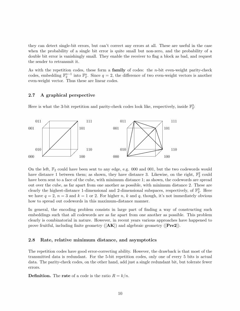
2.7 A graphical perspective

Here is what the 3-bit repetition and parity-check codes look like, respectively, inside F32:

��

��

��

��

000 100

001 101

010 110

011 111

����������

��

��

��

��

000 100

001 101

010 110

011 111

��������

����������

PPPPPP

BBBBBB

@@@

@@

@@@

On the left, F2 could have been sent to any edge, e.g. 000 and 001, but the two codewords wouldhave distance 1 between them; as shown, they have distance 3. Likewise, on the right, F2

2 couldhave been sent to a face of the cube, with minimum distance 1; as shown, the codewords are spreadout over the cube, as far apart from one another as possible, with minimum distance 2. These areclearly the highest-distance 1-dimensional and 2-dimensional subspaces, respectively, of F3

2. Herewe have q = 2, n = 3 and k = 1 or 2. For higher n, k and q, though, it’s not immediately obvioushow to spread out codewords in this maximum-distance manner.

In general, the encoding problem consists in large part of finding a way of constructing suchembeddings such that all codewords are as far apart from one another as possible. This problemclearly is combinatorial in nature. However, in recent years various approaches have happened toprove fruitful, including finite geometry ([AK]) and algebraic geometry ([Pre2]).

2.8 Rate, relative minimum distance, and asymptotics

The repetition codes have good error-correcting ability. However, the drawback is that most of thetransmitted data is redundant. For the 5-bit repetition codes, only one of every 5 bits is actualdata. The parity-check codes, on the other hand, add just a single redundant bit, but tolerate fewererrors.

Definition. The rate of a code is the ratio R = k/n.

10

The repetition codes have rate R = 1/n. As n increases, R approaches zero. The parity-checkcodes have rate R = (n− 1)/n, which approaches 1 as n increases.

Definition. The relative minimum distance of a code is the ratio δ = d/n.

The repetition codes have relative minimum distance δ = n/n = 1. The parity-check codes haverelative minimum distance 2/n, which approaches 0 as n increases.

Of course, R and δ are both confined to the unit interval. We say that asymptotically (as ngets big) the repetition-code family has R = 0 and δ = 1; asymptotically the parity-check familyhas R = 1 and δ = 0. For large n, the repetition codes carry vanishingly little actual data; theiroverhead is too large. For large n, the parity-check codes detect vanishingly few errors per block;their overhead is too small.

Definition. A good code (really, a good family of codes) is one whose asymptotic rate andasymptotic relative minimum distance are both bounded away from zero.

Clearly, the repetition and parity-check codes are not good. It can be shown that good codes exist;see [MS] for examples.

2.9 Code parameters; upper and lower bounds

A linear code is parameterized by the four integers n, k, d and q, or equivalently by the four rationalnumbers n, R, δ and q. Sometimes one says that C is an [n, k, d] code, or perhaps an [n, k, d]qcode. For example, the 5-bit binary repetition code is a [5, 1, 5]2 code. (Similarly, we might writean asymptotic parameterization of a family of codes as [R, δ] or [R, δ]q.)

We encode by embedding Fkq into Fn

q . Not any embedding will do: as we saw in section 2.7, thecanonical injection which appends n − k zeroes is an embedding, but it has minimum distance 1.We want to find an embedding which keeps the vectors as far apart from one another as possible,maximizing d, in order to maximize the code’s error-control ability. Or, given a fixed minimumdistance, we would like to minimize n or maximize k, to keep the code’s rate high. Ideally wewould like the rate and the relative minimum distance to both be high, but there are results (see[MS], [PW], [Wal]) which show that there are upper bounds on the asymptotic rate and relativeminimum distance.

Both R and δ are in the unit interval, so we may think of a parameter space which looks like theunit square:

Asymptotic Singleton upper bound�

Good codes exist�

Asymptotic Plotkin upper bound�

Unattainable ideal�s

Repetition codes�s

Parity-check codes - sR

@@@@@@@@

AAAAAAAA

δ

11

Note that there are particular codes with parameters in various places on this square. The zero-appending code, given by the map from Fq to Fn

q which appends n − 1 zeroes, has R = 1/n andδ = 1/n. Asymptotically, both are zero. Also, the identity code with n = k = 1 has R = 1 andδ = 1. However, this has no error-control ability at all.

The Singleton bound states that for all codes, d ≤ n− k + 1. Thus, for any code with n > 1, theR = 1, δ = 1 corner is unattainable. Asympotically, the Singleton bound shows that R + δ ≤ 1.This means that the asymptotic (R, δ) of a family of codes must be below the main diagonal.Clearly, this applies to even the identity codes, for which R = 1 but δ → 0. The Plotkin boundshows that the asymptotic (R, δ) must be below the lower diagonal as well, where the δ interceptis 1− 1/q. See [Wal] for a lucid discussion of these and other bounds.

The Singleton and Plotkin bounds provide upper limits on the best code families: no codes canbe asymptotically better. There are also lower bounds which specify how good the best codescan be, but don’t constrain how bad the worst codes can be (for example, the zero-appending codementioned above). One proves a lower bound, showing that there exist codes with (R, δ) abovesome curve in R, δ space; the problem of actually producing such codes is another problem entirely.Both of these issues are topics of research.

12

3 Encoding

3.1 The generator matrix

Up to now we haven’t really put much linear algebra to work. To facilitate analysis, we now requirenot only that we have linear block codes mapping injectively from Fk

q into Fnq , but furthermore that

the injective mapping is a vector-space homomorphism, i.e. a linear transformation. There aremany advantages to using a linear transformation, not the least of which is that instead of havingto remember qk images for all the message words, we need to remember only the images of k basisvectors.

Such a linear transformation exists for any linear code. For example, {000, 100, 010, 110} is asubspace of F3

2, but I can send F22 into it by 00 7→ 110, 01 7→ 100, 10 7→ 000, 11 7→ 010. This is

a 1-1 map but it isn’t linear since it doesn’t send zero to zero. As long as I don’t insist on whichelements of Fk

q map to which elements of C, though, I can produce a linear map: since Fkq and C

are vector spaces of the same dimensions over the same field, an isomorphism exists. To obtainit explicitly if only C is given, form a tall matrix the rows of which are all the vectors of C, thenrow-reduce and discard zero rows. The result is a basis for C. Then, send the ith standard basisvector in Fk

q to the ith basis vector of C.

However it is obtained, we write a generator matrix

G : Fkq → Fn

q

where C is the image of G in Fnq . For convenience later on (although it seems quite strange at the

moment), we write G as a k×n matrix: to encode the message word m, we write mG rather thanGm. (If this seems awkward, you may wish to temporarily think in terms of an n × k generatormatrix, then transpose it when you’re done. Also, from the context it is clear whether I’m treatingm as a row or column vector.)

What is a generator matrix for the repetition codes? Clearly, we write (n = 5 here)

G =[

1 1 1 1 1]

For the parity-check code, we want (with n = 5)

[a, b, c, d, a + b + c + d

]=

[a, b, c, d

] 1 0 0 0 10 1 0 0 10 0 1 0 10 0 0 1 1

so

G =

1 0 0 0 10 1 0 0 10 0 1 0 10 0 0 1 1

Of course, when εi is the ith standard basis vector for Fk

q , εiG is the ith row of G. Unless k = 1and q = 2, there will be more than one basis vector, hence more than one permutation of the

13

basis, along with various linear combinations of the basis vectors. Thus the generator matrix isgenerally not unique. Two different generator matrices are equivalent, though, if they generate thesame subspace C of Fn

q . To test for equivalence of two generator matrices, test for equality of theirrow-echelon forms.

(Computational note: finite fields have the property that computer arithmetic is exact. Thus, thereis no roundoff error, and algorithms such as row reduction may be implemented easily for finitefields, with naive pivoting.)

3.2 Systematic codes

We’ve been saying that a linear code C is a k-dimensional subspace of Fnq . From this definition,

G could take any form as long as it has rank k. However, our two examples so far (repetitionand parity-check codes) have an additional property: the first k bits of each n-bit codeword areidentical to the k bits of the corresponding message word.

Definition. A linear code is systematic if its generator matrix G is of the form [Ik|A] for somek × (n− k) matrix A, where Ik is the k × k identity matrix.

Any linear code can be made systematic: just put G in row-echelon form.

14

4 Decoding

4.1 The parity-check matrix

If a linear code C has been chosen, we’ve just seen that encoding is easy: it’s just matrix multipli-cation. But how do we decode, and moreover, how do we do so efficiently? This might seem to bea harder problem. In fact, in general it is. There have been codes which were published before anydecoding algorithm was known. And even for well-known codes, one area of current research is todevelop improved decoding algorithms.

Below, it will be useful to find a so-called parity-check matrix, H, such that C is precisely thekernel of H. (The terminology originally comes from parity-check codes, but it is a poor choice ofwords: all linear codes, not just the parity-check ones, have a parity-check matrix.) That is, wewill want Hv to be zero if and only if v is in C. By the rank-nullity theorem, H will necessarilybe (n− k)× n. Unlike with G, we post-multiply, i.e. we write Hv, not vH.

How can such a matrix H be constructed, given G? First, some terminology.

Definition. The dual code of C, written C⊥, is the set of vectors in Fnq which are orthogonal to

all vectors of C, using the standard dot product. (Note that the term dual code here has nothingto do with the term dual space from linear algebra.) That is,

C⊥ = {v ∈ Fnq : u · v = 0 for all u ∈ C}

(The Hamming weight is a vector-space norm, if we define |c| on Fq to have value 0 when c = 0,1 otherwise. If we use the standard dot product, then Fn

q satisfies all the axioms for an innerproduct space except for the positive-definiteness of the dot product. E.g. if Fq has characteristic2, the non-zero vector (1, 1) dotted with itself is 1 + 1 = 0. Note that the Hamming weight iscomputed in Z: it is the number of non-zero coordinates in a vector. However, the dot productis computed in Fq. Thus the Hamming weight and Hamming distance are positive definite, whilethe dot product is not. This means that inner-product-space results such as Fn

q = C ⊕ C⊥ do notapply: the intersection of a subspace and its perp can contain more than just the zero vector. Infact, a code can be self dual, i.e. C = C⊥. For example, {00, 11} is a self-dual subspace of F2

2.From the result immediately below, a self-dual code must have even n, and k must be n/2.)

We already have G; it remains to actually compute a matrix for H. Suppose that our problemwere reversed, i.e. if we had H, how would we compute G? That’s easy: since the kernel of His the image of G (which is C) we could just compute the kernel basis of H, which is a standardelementary linear algebra problem. G would have rows equal to the elements of that basis.

Now, I claim that, fortuitously, the generator matrix of C⊥ is H and the parity-check matrix ofC⊥ is G. That is, C⊥’s G and H are swapped from C’s. Also note that (C⊥)⊥ is just C. We aregiven G, which is C’s generator matrix as well as C⊥’s parity-check matrix. The kernel basis of Gis the generator matrix for C⊥, which is also the parity-check matrix for C. So this trick meansthat not only can we get a G by computing a kernel basis of an H, but vice versa as well.

It remains to prove that C⊥ has generator matrix H and parity-check matrix G. Remember the

15

convention that a generator matrix acts by post-multiplication and that a parity-check matrix actsby pre-multiplication. So in this role, H maps Fn−k

q to Fnq by sending z to zH, and G maps Fn

q toFk

q by sending v to Gv. To avoid confusion (only for the duration of this proof) we will write ·Gfor G : Fk

q → Fnq acting by post-multiplication and G· for G : Fn

q → Fkq acting by pre-multiplication.

Likewise, we will write H· for H : Fnq → Fn−k

q and ·H for H : Fn−kq → Fn

q . Plain G and H refer tothe matrices without respect to a linear transformation.

We want the following short exact sequences:

0→ Fkq

·G→ Fnq

H·→ Fn−kq → 0

0← Fkq

G·← Fnq

·H← Fn−kq ← 0

with im(·G) = C = ker(H·) and im(·H) = C⊥ = ker(G·). The short exactness means that ·G and·H are 1-1, while H· and G· are onto. Thus, it suffices to show: (1) im(·H) = C⊥; (2) ·H is 1-1,(3) ker(G·) = C⊥, and (4) G· is onto. Now, we already have that the matrix G has rank k and Hhas rank n − k. Since row rank equals column rank, (4) will follow from (3) by the rank-nullitytheorem. Likewise, (2) will follow from (1) since C⊥ has dimension n− k.

To prove (3), first let v ∈ C⊥. The rows of G form a basis for C; let gi be the ith row of G, fori = 1, . . . , k, where each gi is a vector of length n (since it is in Fn

q ). Also let v = (v1, . . . , vn). Thematrix-times-vector multiplication G · v consists of dot products of v with the rows of G:

G · v =

g1...

gk

v1

...vn

=

g1 · v...

gk · v

Since each gi is in C and since v is in C⊥, all the dot products are zero and so G · v = 0.

Conversely, let v ∈ ker(G·). Then G · v = 0. Again, this product consists of dot products of rowsof G with v, so gi · v = 0 for all gi’s. Let c be an arbitrary element of C. Since the gi’s are a basisfor C, c =

∑ki=1 cigi for some ci’s in Fq. Then

v · c = v ·k∑

i=1

cigi

=k∑

i=1

ci(v · gi) = 0

Therefore v ∈ C⊥.

To prove that im(·H) = C⊥, notice in general that when a matrix X acts on a standard basis byXεi, the image of that basis consists of the columns of X. Likewise, when X acts on a standardbasis by εiX, the image of that basis consists of the rows of X. It will suffice to show that the rows

16

of H are a basis for C⊥. Remember that we set up H to check the elements of C, and since G hasrows forming a basis for C, necessarily

HGt = 0

This means that the rows of H are orthogonal to the rows of G, which shows that the rows of Hare in C⊥. Since we know that H has rank n− k, the image of the standard basis for Fn−k

q under·H is linearly independent, and im(·H) must be all of C⊥.

Example. Let’s carry out this computation for the two families of codes we’ve seen so far. The5-bit repetition code has generator matrix

G =[

1 1 1 1 1]

We then compute the kernel basis (in row-echelon form)

H =

1 0 0 0 10 1 0 0 10 0 1 0 10 0 0 1 1

Intuitively, this makes sense: recalling that we are working mod 2, this means that Hv is 0 onlywhen v has all coordinates the same. The two possible cases are 00000 and 11111, which areprecisely the codewords of the 5-bit repetition codes.

Next, the 5-bit parity-check code has generator matrix

G =

1 0 0 0 10 1 0 0 10 0 1 0 10 0 0 1 1

We then compute

H =[

1 1 1 1 1]

Intuitively, this also makes sense: pre-multiplying v by H just adds up the bits of v mod 2. Theresult will be zero precisely when v has even parity, which is the case iff v is in C.

As an added bonus, since the first G is the same as the second H, and vice versa, we now see thatthe repetition and parity-check families are duals of one another.

4.2 Computing H for systematic codes

The parity-check matrix is particularly easy to compute when C is systematic, i.e. when G is inrow-echelon form. For example, take k = 3, n = 6 and suppose

G = [Ik|A] =

1 0 0 a14 a15 a16

0 1 0 a24 a25 a26

0 0 1 a34 a35 a36

17

Writing Gtm rather than mG to save horizontal space on the paper, a message word (m1,m2,m3)is encoded as

1 0 00 1 00 0 1

a14 a24 a34

a15 a25 a35

a16 a26 a36

m1

m2

m3

=

m1

m2

m3

a14m1 + a24m2 + a34m3

a15m1 + a25m2 + a35m3

a16m1 + a26m2 + a36m3

We want to write an H such that H times this codeword is zero, but that’s easy:

−a14 −a24 −a34 1 0 0−a15 −a25 −a35 0 1 0−a16 −a26 −a36 1 0 1

m1

m2

m3

a14m1 + a24m2 + a34m3

a15m1 + a25m2 + a35m3

a16m1 + a26m2 + a36m3

=

000000

We can generalize this example to see that if

G = [Ik|A]

thenH = [−At|In−k]

Thus, systematic G and H may be computed from one another by inspection.

4.3 Brute-force decoding

If I send you an encoded message, with errors in transit, how do you decode to find out what Ireally meant to say? If the message space is small, i.e. if q and n are small, then you could simplymake a list of all possible elements of Fn

q , with the nearest-neighbor codeword precomputed byhand for each. This is what we did in section 2.5. However this is infeasible for larger codes, whichmight have billions of codewords or more: it requires having a table of size qn.

4.4 The coat of arms

A useful diagram from [MS], attributed therein to David Slepian, is the following:

18

Sender - Encoder - Channel - Decoder - Recipient

m = m1 · · ·mk

Messageu = u1 · · ·un

Codeword

e = e1 · · · en

6

6

����

Error vector

v = u + e

Received vectore = e1 · · · en

Estimate oferror

m = m1 · · · mk

Estimate of message

Since we are assuming our channel only inserts random errors, without changing the block lengthby loss of synchronization, we can think of the error vector as being added to the codeword duringtransmission. Since we embed our Fk

q into Fnq using a linear transformation (rather than any old

injective map), and since Hu is zero for all codewords u, we have the following key fact:

v = u + e

Hv = H(u + e) = Hu + He = He

4.5 Standard-array decoding

Definition. The quantity Hv = He from the previous section is called the syndrome of v.

When we form the quotient space Fnq /C, from elementary algebra we know that the cosets of C

partition Fnq . Since C is precisely the kernel of H, if two received vectors are in the same coset,

u ∼ v

u− v ∈ C

H(u− v) = 0Hu = Hv

Thus, two vectors are in the same coset iff they share the same syndrome.

Now, u was transmitted; v = u+e was received, but the receiver can only guess at what e is. Sincev and e have the same syndrome, the true error vector e is somewhere in v’s coset. Furthermore,since we are using the maximum likelihood assumption mentioned in section 2.1, the most likelyerror vector e is the smallest-weight vector in v’s coset. (A decoding error means e 6= e.)

So, the standard-array decoding algorithm has two stages: the first stage is some precompu-tation before any data is received; the second is done as each block is received.

Precomputation stage:

• Write down the elements of Fkq and encode each element. This is a two-by-qk table, pairing

up message words and codewords. Sort this by codeword for easy lookup later.

19

• Write down the quotient space Fnq /C. This requires making, for the moment, a matrix of all

qn elements of Fnq . (Note that this algorithm is also not OK for large codes, although the

resulting tables will be smaller than for the brute-force method.)

• For each coset, search for the smallest-weight element in the coset. This is called the cosetleader. Compute and remember the syndrome of the coset leader; forget about the rest ofthe coset.

• Make a list pairing up syndromes and coset leaders. This is a two-by-qn−k table. Sort thisby syndrome for easy lookup later.

Decoding stage:

• Given a received vector v, compute its syndrome s.

• Look up this syndrome in the precomputed syndrome/leader table.

• Find the most likely error vector e corresponding to s.

• Compute u = v − e.

• Look up u in the precomputed message/codeword table to obtain m. This is our best guessof what the transmitter sent.

Note that both table lookups are done on sorted data. This means we don’t have to sequentiallyscan either table at run time. The syndromes are all of Fn−k

q , so we can use base-q arithmetic togo directly to the desired element of the syndrome/leader table. For the message/codeword table,we can use a binary search, with a number of lookups roughly log2 of the table size.

(Note that the message/codeword table isn’t necessary. Once we have a codeword u, we can solvethe linear system u = mG for m using row reduction. This reduces table space, at the expense ofmaking the decoding stage use more computation.)

Example. Let’s compute the standard array for the 3-bit repetition code. We have

G =[

1 1 1], H =

[1 0 10 1 1

]The message words are 0 and 1. Their images under G are 000 and 111. So, the message/codewordtable is as follows:

m u

0 0001 111

The possible received vectors (all of Fnq ) are:

000, 001, 010, 011, 100, 101, 110, 111

20

C is:000, 111

Fnq /C is:

{000, 111},{010, 101},{100, 011},{001, 110}

The coset leaders are the minimum-weight vectors of each coset. These are as follows, with corre-sponding syndromes:

e s

000 00010 01100 10001 11

Here is an example of using the standard array to decode a received vector:

• Receive v = 011.

• Compute s = Hv = 10

• 10 in binary is 2 in decimal, so go to row 2 (with row indices starting at 0) of the syn-drome/leader table.

• At that spot, find e = 100.

• Compute u = v − e = 011− 100 = 111.

• Match codeword 111 with message word 1 in the message/codeword table to obtain m = 1.

21

5 The binary Hamming and simplex codes

Having seen the repetition and parity-check codes, we will now round out our set of simple exampleswith two more families.

Above we saw that for a linear code C with parity-check matrix H, if v = u + e is the receivedvector, then Hv = He. In the special case q = 2, though, more may be said. In this case, all theerror bits are 0 or 1. Letting εj be the standard basis for Fn

q , i.e. εj has a 1 in the jth spot andzeroes elsewhere,

e =n∑

j=1

cjεj

where all the cj ’s are zero or one. Then

He = H

n∑j=1

cjεj

=n∑

j=1

cjHεj

=n∑

j=1

cjHj

where we write Hj for the jth column of H. That is, for a binary code, the syndrome is the sum ofthe columns of H where an error occurred. If we only wish to be able to correct a single-bit error,then we may assume that e has at most a single 1-bit. In that case, if v is a codeword, then Hvwill be the zero vector, but if v is not a codeword, then Hv will be Hj where j is the position ofthe error bit. One way to make this easy is to simply make a parity-check matrix whose columnsencode all possible error positions. For example,

H =

0 0 0 1 1 1 10 1 1 0 0 1 11 0 1 0 1 0 1

Column 1 is 001 which is binary for 1; column 2 is 010 which is binary for 2; etc. (There is nocolumn equal to 000, since a column of zeroes has no effect on the syndrome.)

Let r be the number of rows of H; the number of columns is 2r − 1. Since H is an (n − k) × nmatrix, the binary Hamming codes have k = 2r − 1− r and n = 2r − 1. As n gets big, R = k/ngoes to 1. The binary Hamming codes have minimum distance 3: notice that 1110 · · · 0 is alwaysa codeword, so d ≤ 3; meanwhile, the Hamming codes are single-error-correcting so d ≥ 3. Thisforces d = 3, and δ = d/n goes to zero as n gets big. Thus, Hamming codes are not good codes.However, the decoding algorithm is fantastically simple.

The duals of the binary Hamming codes are called binary simplex codes. As discussed in [MS],in the simplex codes all pairs of distinct non-zero vectors are the same distance from one another,namely, 2r−1. There are 2r elements in the r simplex code, so these are [2r − 1, r, 2r−1] codes.Asymptotically, they have R = 0 and δ = 1/2.

22

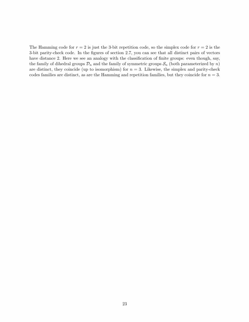
The Hamming code for r = 2 is just the 3-bit repetition code, so the simplex code for r = 2 is the3-bit parity-check code. In the figures of section 2.7, you can see that all distinct pairs of vectorshave distance 2. Here we see an analogy with the classification of finite groups: even though, say,the family of dihedral groups Dn and the family of symmetric groups Sn (both parameterized by n)are distinct, they coincide (up to isomorphism) for n = 3. Likewise, the simplex and parity-checkcodes families are distinct, as are the Hamming and repetition families, but they coincide for n = 3.

23

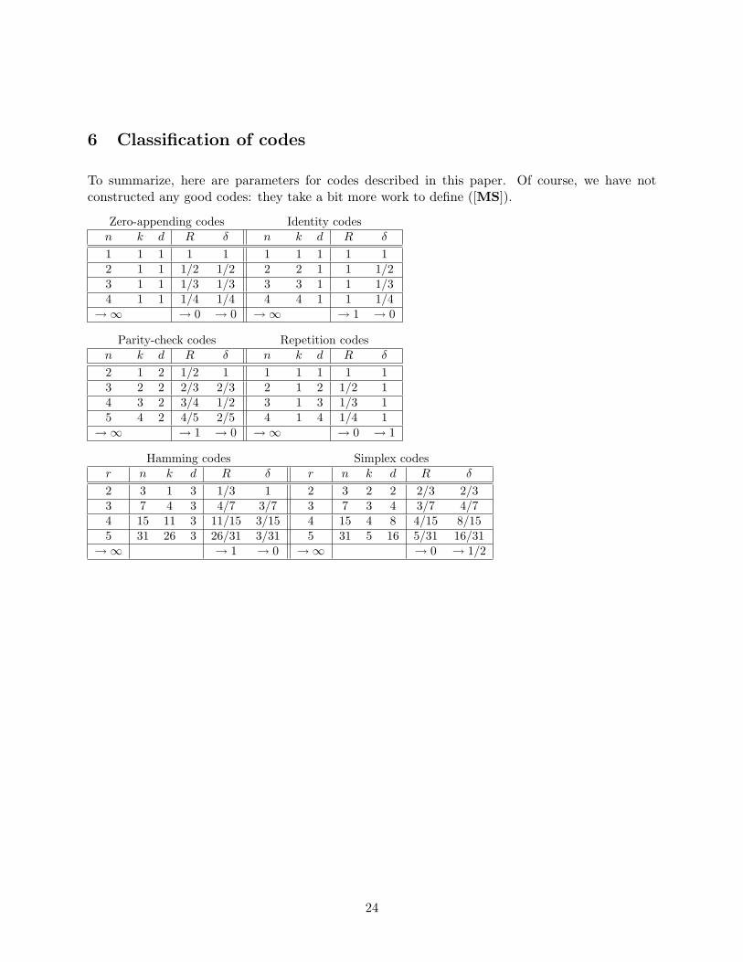
6 Classification of codes

To summarize, here are parameters for codes described in this paper. Of course, we have notconstructed any good codes: they take a bit more work to define ([MS]).

Zero-appending codes Identity codesn k d R δ n k d R δ

1 1 1 1 1 1 1 1 1 12 1 1 1/2 1/2 2 2 1 1 1/23 1 1 1/3 1/3 3 3 1 1 1/34 1 1 1/4 1/4 4 4 1 1 1/4→∞ → 0 → 0 →∞ → 1 → 0

Parity-check codes Repetition codesn k d R δ n k d R δ

2 1 2 1/2 1 1 1 1 1 13 2 2 2/3 2/3 2 1 2 1/2 14 3 2 3/4 1/2 3 1 3 1/3 15 4 2 4/5 2/5 4 1 4 1/4 1→∞ → 1 → 0 →∞ → 0 → 1

Hamming codes Simplex codesr n k d R δ r n k d R δ

2 3 1 3 1/3 1 2 3 2 2 2/3 2/33 7 4 3 4/7 3/7 3 7 3 4 3/7 4/74 15 11 3 11/15 3/15 4 15 4 8 4/15 8/155 31 26 3 26/31 3/31 5 31 5 16 5/31 16/31→∞ → 1 → 0 →∞ → 0 → 1/2

24

7 More information

The three most fundamental papers (dating from 1948-1950) are [Sha], [Ham], and [Gol].

There are many introductions to coding theory, of which I mention a few: see [MS] and [Ber] for athorough treatment of elementary as well as advanced topics. [VO] and [Pre1] are less encyclopedicand more elementary. [MS] discusses only block codes, and does so in depth; [PW] discusses blockand tree codes. See [Sud] for an algorithmic approach.

Topics of research in coding theory include the following:

• New families of codes, including some highly mathematical approaches (e.g. [Pre2]).

• Sharper bounds.

• More efficient decoding algorithms.

• Non-linear codes.

• Codes over non-fields (e.g. [HKCSS]).

[MS] contains many open problems. [Sud] has a large bibliography; [MS] has a huge bibliography.

8 Acknowledgements

The presentation here is more or less from the first chapters of [MS], [PW], [Ber], and [VO].However, given that my intended audience is mathematics students rather than electrical engineers,I have chosen to write a more algebraic treatment.

25

References

[AK] Assmus, E.F. and Key, J.D. Designs and Their Codes. Cambridge University Press, 1994.

[Ber] E. Berlekamp. Algebraic Coding Theory (revised 1984 edition). Aegean Park Press, 1984.

[Gol] Golay, M.J.E. Notes on digital coding. Proceedings of the IRE, 37:657, June 1949.

[Gib] Gibbs, W.W. The Network in Every Room. Scientific American, February 2002.

[Ham] Hamming, R.W. Error Detecting and Error Correcting Codes. Bell System TechnicalJournal, 29:147-160, April 1950.

[HKCSS] Hammons, A.R. et al. The Z4-Linearity of Kerdock, Preparata, Goethals and RelatedCodes. http://www.research.att.com/~njas/doc/linear.ps

[LN] R. Lidl and H. Niederreiter. Finite Fields. Cambridge University Press, 1997.

[MS] MacWilliams, F.J. and Sloane, N.J.A. The Theory of Error-Correcting Codes. ElsevierScience B.V., 1997.

[PW] Peterson, W.W. and Weldon, E.J. Error-Correcting Codes (2nd ed.). MIT Press, 1972.

[Pre1] Pretzel, O. Error-Correcting Codes and Finite Fields. Oxford University Press, 1996.

[Pre2] Pretzel, O. Codes and Algebraic Curves. Oxford University Press, 1998.

[Sha] Shannon, C.E. A mathematical theory of communication. Bell System Technical Journal,27:379-423, 623-656, 1948.

[Sud] Sudan, M. Algorithmic Introduction to Coding Theory.http://theory.lcs.mit.edu/~madhu/coding/ibm

[VO] Vanstone, S.A. and van Oorschot, P.C. An Introduction to Error Correcting Codes withApplications. Kluwer Academic Publishers, 1989.

[Wal] Walker, J. Codes and Curves.http://www.math.unl.edu/~jwalker/papers/rev.pdf

26

27

Index

Aalphabet . . . . . . . . . . . . . . . . . . . . . . . . . . . . . . . . . . . . . 4asymptotically . . . . . . . . . . . . . . . . . . . . . . . . . . . . . .11

Bbinary codes . . . . . . . . . . . . . . . . . . . . . . . . . . . . . . . . . 6binary symmetric channel . . . . . . . . . . . . . . . . . . . .6bits . . . . . . . . . . . . . . . . . . . . . . . . . . . . . . . . . . . . . . . . . .4block code . . . . . . . . . . . . . . . . . . . . . . . . . . . . . . . . . . . 7block codes . . . . . . . . . . . . . . . . . . . . . . . . . . . . . . . . . . 4burst error . . . . . . . . . . . . . . . . . . . . . . . . . . . . . . . . . . .5

Cchannel capacity . . . . . . . . . . . . . . . . . . . . . . . . . . . . . 6channel coding . . . . . . . . . . . . . . . . . . . . . . . . . . . . . . .5code . . . . . . . . . . . . . . . . . . . . . . . . . . . . . . . . . . . . . . . . . 7codeword . . . . . . . . . . . . . . . . . . . . . . . . . . . . . . . . . . . . 7coding . . . . . . . . . . . . . . . . . . . . . . . . . . . . . . . . . . . . . . . 4convolutional codes . . . . . . . . . . . . . . . . . . . . . . . . . . 5correct . . . . . . . . . . . . . . . . . . . . . . . . . . . . . . . . . . . . . . 9coset leader . . . . . . . . . . . . . . . . . . . . . . . . . . . . . . . . .20

Ddecode . . . . . . . . . . . . . . . . . . . . . . . . . . . . . . . . . . . . . . .4decoding error . . . . . . . . . . . . . . . . . . . . . . . . . . . 9, 19detect . . . . . . . . . . . . . . . . . . . . . . . . . . . . . . . . . . . . . . . 9dimension . . . . . . . . . . . . . . . . . . . . . . . . . . . . . . . . . . . 7dual code . . . . . . . . . . . . . . . . . . . . . . . . . . . . . . . . . . .15

Eembedding . . . . . . . . . . . . . . . . . . . . . . . . . . . . . . . . . . .7encode . . . . . . . . . . . . . . . . . . . . . . . . . . . . . . . . . . . . . . .4encoding problem . . . . . . . . . . . . . . . . . . . . . . . . . . . . 7error control . . . . . . . . . . . . . . . . . . . . . . . . . . . . . . . . . 4even-weight . . . . . . . . . . . . . . . . . . . . . . . . . . . . . . . . . . 9

Ffamily . . . . . . . . . . . . . . . . . . . . . . . . . . . . . . . . . . . 7, 10

Ggenerator matrix . . . . . . . . . . . . . . . . . . . . . . . . . . . 13good code . . . . . . . . . . . . . . . . . . . . . . . . . . . . . . . . . . 11

H

Hamming codes . . . . . . . . . . . . . . . . . . . . . . . . . . . . 22Hamming distance . . . . . . . . . . . . . . . . . . . . . . . . . . . 7Hamming weight . . . . . . . . . . . . . . . . . . . . . . . . . . . . 7

Llength . . . . . . . . . . . . . . . . . . . . . . . . . . . . . . . . . . . . . . . 7linear code . . . . . . . . . . . . . . . . . . . . . . . . . . . . . . . . . . .7lower bounds . . . . . . . . . . . . . . . . . . . . . . . . . . . . . . . 12

Mmaximum likelihood . . . . . . . . . . . . . . . . . . . 6, 8, 19message word . . . . . . . . . . . . . . . . . . . . . . . . . . . . . . . . 7messages . . . . . . . . . . . . . . . . . . . . . . . . . . . . . . . . . . . . 4minimum distance . . . . . . . . . . . . . . . . . . . . . . . . . . . 8minimum weight . . . . . . . . . . . . . . . . . . . . . . . . . . . . . 8

Pparity check . . . . . . . . . . . . . . . . . . . . . . . . . . . . . . . . . 9parity-check matrix . . . . . . . . . . . . . . . . . . . . . . . . . 15

Rrandom errors . . . . . . . . . . . . . . . . . . . . . . . . . . . . . . . 5rate . . . . . . . . . . . . . . . . . . . . . . . . . . . . . . . . . . . . . . . . 10received word . . . . . . . . . . . . . . . . . . . . . . . . . . . . . . . . 7relative minimum distance . . . . . . . . . . . . . . . . . . 11repetition code . . . . . . . . . . . . . . . . . . . . . . . . . . . . . . 7

Sself dual . . . . . . . . . . . . . . . . . . . . . . . . . . . . . . . . . . . . 15Shannon’s theorem . . . . . . . . . . . . . . . . . . . . . . . . . . 6simplex codes . . . . . . . . . . . . . . . . . . . . . . . . . . . . . . .22Singleton bound . . . . . . . . . . . . . . . . . . . . . . . . . . . . 12source coding . . . . . . . . . . . . . . . . . . . . . . . . . . . . . . . . 5standard-array decoding algorithm . . . . . . . . . .19synchronization errors . . . . . . . . . . . . . . . . . . . . . . . 5syndrome . . . . . . . . . . . . . . . . . . . . . . . . . . . . . . . . . . .19systematic . . . . . . . . . . . . . . . . . . . . . . . . . . . . . . . . . . 14

Ttree codes . . . . . . . . . . . . . . . . . . . . . . . . . . . . . . . . . . . 5true minimum distance . . . . . . . . . . . . . . . . . . . . . . 8

Uupper bounds . . . . . . . . . . . . . . . . . . . . . . . . . . . . . . .11

28