An Intertemporal General Equilibrium Model of Asset Prices - A short...
23
An Intertemporal General Equilibrium Model of Asset Prices A short review by Cox, Ingersoll, and Ross November 20, 2012 1 / 23
Transcript of An Intertemporal General Equilibrium Model of Asset Prices - A short...
An Intertemporal General EquilibriumModel of Asset Prices
A short review
by Cox, Ingersoll, and Ross
November 20, 2012
1 / 23

Introduction
• Merton (1973) analyzes a continuous time,consumption-based asset pricing model. It makesparametric assumptions on the price processes, andthere is no production in the economy.
• Lucas (1978) analyzes a discreet time,consumption-based model. It allows production, doesnot make parametric assumptions on how to priceassets, and is a general equilibrium model.
• There is a companion paper by the same authors thatdiscusses a specialization of the model in this paper.
2 / 23

The setup
The economy has
1. production processes; n of them
2. contingent claims; a lot of them, and the exactnumber is not important
Agents makes the following decisions
1. how to consume; {ct : t > 0} = c
2. how to invest in assets; {at : t > 0} = a
3. how to invest in claims; {bt : t > 0} = b
The economy equilibrates and determines
1. interest rate; r
2. expected rate of return of claims; β
3 / 23

Parametric assumptions of the economy
• The state variables Y has the dynamics
dY (t) = µ(Y, t)dt+ S(Y, t)dw(t)
• The production technology
I−1η dη(t) = α(Y, t)dt+G(Y, t)dw(t)
• The contingent claims
dF i(t) = [F i(t)βi(t)− δi(t)] + F i(t)hidw(t)
But note that β is an endogenous process.
4 / 23

The representative agent optimizes theinvestment and consumption
There is a state and time dependent utility function
U(ct, Yt, t),
and the agent makes the following decision at each t
1. at; investment in productive assets
2. bt; investment in auxiliary assets
3. ct; consumption
We refer to the triple (a, b, c) the control process andlabel it v = {vt : t ≥ 0}.
5 / 23
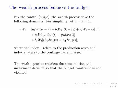
The wealth process balances the budget
Fix the control (a, b, c), the wealth process take thefollowing dynamics. For simplicity, let n = k = 1.
dWt = [atWt(α− r) + btWt(βt − rt) + rtWt − ct] dt+ atWt[g1dw1(t) + g2dw1(t)]
+ btWt[(h1dw1(t) + h2dw1(t)],
where the index 1 refers to the production asset andindex 2 refers to the contingent-claim asset.
The wealth process restricts the consumption andinvestment decision so that the budget constraint is notviolated.
6 / 23

The agent’s optimization problem
The agent solves the following stochastic control problem
supv
E[∫ ∞
0U(cs, Ys, s)ds
]subject to: W0 = w0 and Wt ≥ 0.
Use the hat to denote optimal policy, i.e. v denotes an
optimal control.
7 / 23

Solving agent’s problem (1): Dynamicprogramming principal (DPP)
Define the value function J as
J(t, w, y) = supv
E[∫ ∞
tU(cs, Ys, s)ds
]subject to: Wt = w and Yt = y
Then locally, the optimality condition becomes
J(t, w, y) = supv
E[∫ τ
tU(cs, Y
w,ys , s)ds+ J(τ,Ww,y
τ , Y w,yτ )
]
8 / 23

Solving agent’s problem (2): HJB-PDE
With DPP, Ito’s formula, and the assumption that J issmooth enough, we get the following non-linear PDE
supv
[LvJ + U(v, y, t)] = −Jt,
with some boundary conditions.
9 / 23

Solution of the PDE vs. solution to theoriginal stochastic control problem
lemma (1)
If J is a solution to the PDE and also J is C2, then
1. J is a value function.
2. the v s.t. LvJ +U(v, y, t) = −Jt is an optimal policy.
Note that the Bellman equation by itself is neithersufficient nor necessary.
To find the solution of the stochastic control problem:
1. Solve the PDE
2. Verification step
10 / 23
Solving agent’s problem (3): Resolution
Make the explicit assumption that the value solutiont, w, y 7→ J(t, w, y) exists and is unique.
lemma (2)
J(t, w, y) is increasing and strictly concave in w.
11 / 23

Towards an equilibrium
The equilibrium conditions are:
1.∑
i = ai = 1
2. bi = 0
Then, finding the solution to the agent’s problem andimposing the equilibrium conditions pin down thefollowing processes:
1. r; the interest rate
2. β; the expected return of claims
3. a investment strategy
4. c consumption
12 / 23

Key result (1): Interest rate
Theorem (1)
r(t, w, y) =
1. atα− −JwwJw
var(w)
w−
k∑i=1
−JwyiJw
cov(w, yi)
w
2. − Jwt + LJwJw
= −D[Jw]
Jw
3. atα+
[cov(w, Jw)
wJw
],
where the evaluation is w = Wt and y = Yt.
13 / 23

Key result (2): Determining β
Theorem (2)
(βi − r)F i =
1. [φWφYi · · ·φYk ][F iWFiY1 · · ·F
iYk
]T
2. − cov(F i, Jw)
F iJw
φ(·) is specified in equation (20).
14 / 23

Key result (3): Pricing contingent claims
Theorem (3)
The pricing formula F (t, w, y) satisfies the following PDE
LF (t, w, y) + δt = rtF (t, w, y),
where r is determined by Theorem (1) and L is thedifferential generator.
Note that this PDE and along with boundary conditions,which depends on each particular contingent claim, wouldyield the deterministic pricing formula F (t, w, y).
15 / 23

The equilibrium pricing formula is analogousto the Black-Scholes pricing formula)
In the BS setup, a contingent claim that pays h(XT ) atthe termination time T is priced at
F (t, s) = Et,x[e∫ Tt −rdsh(XT )
].
Then, a Feynman-Kac type argument would require thatF (t, s) would also satisfy the PDE
LF (t, s) = rF (t, s),
with terminal condition
f(T, s) = h(s), for all s.
16 / 23

Lemma 3 makes this connection precise
lemma (3)
The solution to the pricing PDE with the boundarycondition given in (34) can be calculated by the followingexpectation formula,
F (W,Y, t, T ) = E{ Θ(W (T ), Y (T ))[exp{−∫ T
tβudu}]1τ≥T
+ Φ(W (τ), Y (τ), τ)[exp{−∫ τ
tβudu}]1τ<T
+
∫ τ∧T
tδs[exp{−
∫ s
tβudu}]ds }.
17 / 23

Pricing in terms of marginal-utility-weightedexpected value
Theorem (4)
F (W,Y, t, T ) = E{ Θ(W (T ), Y (T ))JW (W (T ), Y (T ), T )
JW (W (t), Y (t), t)1τ≥T
+ Φ(W (τ), Y (τ), τ)JW (W (τ), Y (τ), τ)
JW (W (t), Y (t), t)1τ<T
+
∫ τ∧T
tδsJW (W (s), Y (s), s)
JW (W (t), Y (t), t)ds }.
Roughly, it states that the correct “pricing kernel” is theinter-temporal marginal rate of substitution:JW (W (s),Y (s),s)JW (W (t),Y (t),t) .
18 / 23

Comparing to the Lucas model of a single asset
The lucas model prices the asset with payment stream xtat
pt = Et ∞∑j=t
βju′(xj+1)
u′(xt)xj+1
.
Now consider a similar contingent claim in thecontinuous-time economy in which the asset pays thestream δt without a stopping rule. Then this asset ispriced at
pt = Et[∫ ∞
t
JW (W (s), Y (s), s)
JW (W (t), Y (t), t)δsds
].
The lack of a discounting factor here is due to theassumption on U(t, ·).
19 / 23

Let’s see an application/specialization
1. Restrict U to be log utility, state-independent, andtime-homogeneous after discounting in that
U(c, t) = e−∫ t0 rsdslog(c).
2. Let there be only one state variable with thefollowing dynamics
dY (t) = (ξY (t) + ζ)dt+ ν√Y (t)dw(t).
20 / 23

Solving this model yields theCox-Ingersoll-Ross interest rate dynamics
1. a = (GG′)−1α+ e−e′(GG′)−1αe′(GG′)−1e
(GG′)−1e
2. r satisfies the SDE
drt = κt(θt − rt)dt+ σ√rtdwt,
where κ and θ are defined by some SDEs (see (15) ofthe companionl paper.)
The key result here is that the interest rate process isendogenously determined by an equilibrium model.
21 / 23

The Cox-Ingersoll-Ross interest rate model (1)
The process satisfying
drt = κt(θt − rt)dt+ σ√rtdwt,
is known as a mean-reverting process, a.k.a.Ornstein-Uhlenbeck process.
Given this process, the price of a zero couple bond withduration T , f(t, r), can be valued by solving the followingPDE,
ft(t, r) + κt(θt − rt)fr(t, r) +1
2σ2rfrr(t, r) = rf(t, r).
22 / 23
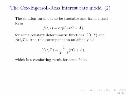
The Cox-Ingersoll-Ross interest rate model (2)
The solution turns out to be tractable and has a closedform
f(t, r) = exp{−rC −A},
for some constant deterministic functions C(t, T ) andA(t, T ). And this corresponds to an affine yield
Y (t, T ) =1
T − t(rC +A),
which is a comforting result for some folks.
23 / 23