AN INTERACTIVE SOFTWARE TOOL TO LEARN ROBUST …€¦ · An Interactive Software Tool to Learn...

An Interactive Software Tool to Learn Robust Control Design Using the QFT Methodology

February 16th, 2007 J.M. Díaz, S. Dormido and J. Aranda 1

AN INTERACTIVE SOFTWARE TOOL TO LEARN ROBUST CONTROL

DESIGN USING THE QFT METHODOLOGY

J. M. Díaz, S. Dormido , J. Aranda

Dpt. de Informática y Automática. ETSI Informática. UNED. Juan del Rosal nº 16. 28040 Madrid. Spain

E-mail: [email protected] [email protected] [email protected]

ABSTRACT

This work presents the main features of QFTIT a new interactive software tool for robust control design

using the QFT methodology. The main advantages of QFTIT compared to other existing tools are its ease

of use and its interactive nature. All that the end-user has to do is to place the mouse pointer over the

different items which the tool displays on the screen. Any action carried out on the screen are

immediately reflected on all the graphs generated and displayed by the tool. This allows the user to

visually perceive the effects of his or her actions during the design of the controller. QFTIT has been

designed bearing in mind the needs of a beginner who wants to learn the QFT methodology as well as the

needs of an advanced user. The tool is freely available in the form of an executable file for Windows or

Mac based platforms. In this paper, a robust control problem is solved with QFTIT in order to describe

the tool.

Keywords: Quantitative feedback theory (QFT); Robust control; Control Systems Computer-Aided

Design (CSCAD), Educational software

1. INTRODUCTION

In the nineties, the spectacular increase in the use of personal computers led to the development of new

software for very different areas. In the field of automatic control, Matlab is without a doubt the most

important software tool. Matlab has a broad set of library functions, “toolboxes”, to implement different

control techniques. In order to use these library functions, users have to write a script file. Users must



therefore have a basic programming knowledge. Once the script has been written, the next step is to

execute it from the Matlab command line and wait for the results. If users want to change some parameter

of their design, they must change some line of script code. Obviously, this way of working is rather

tedious.

From the end of the nineties it has been possible to build graphic user interfaces (GUIs) with Matlab,

which allow Matlab functions to be executed without writing any line of code. Many of the toolboxes

already include these GUIs as an alternative way of working. Basically, the only thing users have to do is

to fill some blank fields with the parameter values and press some button to start the computation.

Moreover, with the Matlab GUI the mouse pointer can drag some graphic element in just one plot.

There are thus two ways of working with the Matlab toolboxes: 1) Writing a script file and invoking it

from the Matlab command line. 2) Using a GUI. These are considered the traditional approach to

analyzing a system or designing a controller.

At present, a new generation of interactive software control packages allow to do an interactive design

with instantaneous performance display. They have created an interesting alternative, called interactive

approach, in comparison with the traditional approach. In this sense innovative and interesting ideas and

concepts were implemented by Prof. Åström and coll. at Lund such as the concept of dynamic pictures

and virtual interactive systems [1]. The main objective of these tools is to involve the users in a more

active way in the analysis and design processes.

In essence, a dynamic picture is a collection of graphical windows that are manipulated simply by using

the mouse. Users do not have to learn or write any sentences. If we change any active element in the

graphical windows an immediate recalculation and presentation automatically begins. In this way we

perceive how these modifications affect the result obtained.

These kinds of tools are based on objects that allow direct graphic manipulation. During these

manipulations, all the objects are immediately updated, not only one as in the Matlab’s GUI. Therefore



the relationship among the objects is continuously maintained. Ictools and CCSdemo [2, 1] developed at

the Department of Automatic Control at Lund Institute of Technology, SysQuake at the Lausanne Federal

Polytechnic School Automatics Institute [3, 4], and Easy Java Simulation developed at the

Department of Mathematics at the University of Murcia [5, 6] are good examples of this new

philosophy to produce a new family of interactive computer-aided design packages in automatic control.

Very often our work as control engineers is reduced to tune some design parameters using a trial and

error procedure following an iterative process. Specifications of the problem are not normally used to

calculate the value of the system parameters because there is not an explicit formula that connects them

directly. This is the reason for dividing, each iteration, into two phases. The first one, often called

synthesis, consists in calculating the unknown parameters of the system taking a group of design

variables (which are related to the specifications) as a basis. During the second phase, called analysis, the

performance of the system is evaluated and compared to the specifications. If they do not agree, the

design variables are modified and a new iteration is performed [7].

It is possible, however, to merge both phases into one and the resulting modification in the parameters

produces an immediate effect. In this way, the design procedure becomes really dynamic and the users

perceive the degree of change in the performance criteria given for the elements that they are

manipulating. This interactive capacity allows us to identify much more easily the objectives that can be

achieved [8, 9].

The interactive approach goes one step further. In many cases, it is not only possible to calculate the

position of a graphic element (be it a curve, a pole, a template or a bound) from the model, controller or

specifications, but also to calculate a new controller from the position of the element. For instance, a

closed loop pole can be computed by calculating the roots of the characteristic polynomial, which itself is

based on the plant and controller; and the controller parameters can be synthesised from the set of closed

loop poles if some conditions on the degrees are fulfilled [10].



This two-way interaction between the graphic representation and the controller allows the manipulation

of the graphical objects with a mouse in a very natural form. Since a good design usually involves

multiple objectives using different representations (time-domain or frequency-domain), it is possible to

display several graphic windows that can be updated simultaneously during the manipulation of the

active elements.

The philosophy of the interactive approach offers two main advantages when compared with the

traditional approach. In the first place, it introduces from the beginning the control engineer to a tight

feedback loop of iterative design. The designers can identify the bottlenecks of their designs in a very

easy way and can attempt to fix them. In second place, and this is probably even more important, not only

is the effect of the manipulation of a design parameter displayed, but its direction and amplitude also

become apparent. The control engineer learns quickly which parameter to use and how to push the design

in the direction of fulfilling better tradeoffs in the specifications. Fundamental limitations of the system

and the type of controller are therefore revealed [11, 12] giving way to finding an acceptable compromise

between all the performance criteria. Using this interactive approach we can learn to recognise when a

process is easy or difficult to control.

This paper describes the main features of the Quantitative Feedback Theory Interactive Tool (QFTIT).

This software tool applies the interactive approach to Quantitative Feedback Theory (QFT) for the first

time. QFT is a very useful robust control design methodology created by I. Horowitz [13]. QFT is a

frequency-domain design method based on two observations: (i) feedback is needed to achieve a desired

plant output response in the presence of plant uncertainty and/or unknown disturbances; and (ii) a

controller that produces less control effort is preferred, i.e., a controller whose bandwidth is smaller is

preferable. QFT is quantitative in the sense that it synthesizes a controller for the exact amount of plant

uncertainty, disturbances and specifications required.

QFT is a very versatile control design technique. It can be used in linear or non-linear systems, invariant

or variant time systems, continuous or discrete systems, and Single Input - Single Output (SISO) or



Multiple Input - Multiple Output (MIMO) systems [13, 14, 15, 16, 17, 18]. Moreover, it is possible to use

QFT on non-minimum phase systems and time-delay systems.

One additional very attractive feature of the QFT technique is the fact that generates narrow bandwidth

controllers, unlike with other robust control techniques (H∞, μ synthesis, LQG/LTR). Furthermore, QFT

usually leads to lower order controllers than other robust control techniques. QFT also deals non-

conservatively with parametric, non-parametric and mixed uncertainty models. It does not assume special

structures for plant uncertainties, disturbances and specifications such as norm-bounded uncertainties,

etc.

On the other hand, the speed at which a QFT design can be performed depends to a great extent on user

experience, while other robust control techniques are less user dependent. Accordingly, QFTIT, thanks to

its ease of use and interactive nature, helps to quickly learn and understand the main concepts of QFT

methodology.

Besides, QFTIT can also be used for advanced users to solve real robust control problem with QFT. In

fact, in [19] QFTIT was successfully used for designing a monovariable robust regulator for the reduction

of motion sickness incidence on a high-speed ferry.

This paper is organised as follows. In section 2 a description of the basic concepts of QFT is included.

Section 3 describes the main features of QFTIT, its advantages and limitations. A comparison of QFTIT

versus others software tool used to implement the QFT methodology is also included. Section 4 describes

the items of the tool and its use by means of the resolution of a simple but illustrative example, a robust

control problem proposed in [20]. Section 5 describes the educational application of QFTIT. Finally

section 5 offers some conclusions, future works and improvements to the tool.

2. BASIC CONCEPTS OF QUANTITATIVE FEEDBACK THEORY

The design procedure using QFT has been described in a wide variety of articles and books [13, 14, 15,

16, 17, 18]. QFT is a methodology used in the design of control systems including uncertainties in the



plant which is subject to external disturbance in the input and output of the plant as well as measurement

noise. Figure 1 illustrates the basic idea behind QFT applied to a SISO system with a control structure

with two degrees of freedom. F is the transfer function of a pre-filter acting on the reference input r. C is

the controller which, depending on an error signal e, generates a control signal u over the set of transfer

functions of the plant P. This set describes the uncertainty region of the plant’s parameters. P may be

subject to disturbances at its input v and/or at its output d. H is the measure sensor of the output signal y,

which may be affected by a measurement noise n.

The QFT method takes into consideration the quantitative information of the plant’s uncertainty, robust

operation requirements, robust tracking, expected disturbance amplitude and the associated damping

requirement.

The controller C must be designed in such a way that the output variations y, which are a consequence of

plant uncertainties P, are within specified tolerance boundaries. Furthermore, the effects of the

disturbances d and v on the output must be acceptably small. On the other hand the pre-filter F is

designed in order to perform the desired control of the reference signal r.

The design is performed using a Nichols diagram, defining a discreet set of trial frequencies Ω. This set is

taken around the desired crossover frequency. As we are treating a family of plant instead of a single

plant, the magnitude and phase of the plants in each frequency correspond to a set of points in the

Nichols diagram. These sets of points forms a connected region or a set of disconnected regions called

“template”. T(ωi) denotes a template computed at the frequency ωi ∈ Ω. A large template implies a

greater uncertainty for a given frequency. The templates and the working specifications are used to define

the domain bounds within the frequency domain. The domain bounds set the limit of the frequency

response of the open loop system.

Each specification contains bound definitions. Bounds are calculated using the corresponding templates

and specifications. The different types of bounds are calculated in the following way:



a) Stability Bounds. By using templates and the specified phase margin.

b) Control Bounds. By using templates and the upper and lower limits of the response in the frequency

domain.

c) Disturbance Bounds. By using the disturbance refusal specifications.

d) Effort control Bounds. By using templates and the specified control limits.

All the bounds computed at the same frequency ωi ∈Ω, associated at the different specifications are

intersecting to generate a final bound B(ωi) which includes the most restrictive regions of all the

considered bounds.

The controller is designed by means of a loop-shaping process in the Nichols diagram. This diagram

sketches the intersection of the bounds calculated for each of the trial frequencies and the characteristics

of the open loop nominal transfer function L0(jω)=C(jω)·P0(jω).

The design is carried out by adding gains, poles and zeroes to the frequency response of the nominal

plant, in order to change the shape of the open loop transfer function. By doing so, the boundaries B(ωi)

are kept for each ωi∈Ω. The controller is the set of all the aforementioned items (gain, poles and zeroes).

Should there be any specification which corresponds to the control of the reference signals, a pre-filter F

must be used. This pre-filter is designed in a similar way as the controller, the difference being in the use

of the limits imposed in the frequency response control. In this case, the shaping may be carried out in the

Bode diagram instead of the Nichols diagram.

The last step for the QFT design is the analysis and validation which includes not only the analysis in the

frequency domain but also the simulations in the temporary domain of the resulting closed loop system.

The benefits of QFT may be summarised as follows:

· The outcome is a robust controller design that is insensitive to plant variation



· There is only one design for the full envelope and it is not necessary to verify plants inside

templates

· Any design limitations are clear at the very beginning

· There is less development time in comparison to other robust design techniques

· QFT generalises classical frequency-domain loop shaping concepts to cope with simultaneous

specifications and plants with uncertainties

· The amount of feedback is adapted to the amount of plant and disturbance uncertainty and to the

performance specifications

· The design trade-offs in every frequency are transparent between stability and performance

specifications. It is possible to determine what specifications are achievable during the early

stages in the design process

· The redesign of the controller for changes in the specifications can be done very fast.

3. MAIN FEATURES OF THE QFTIT INTERACTIVE TOOL

There are currently many different CAD tools [21, 22, 23, 24, 25] all aimed towards helping the designer

to implement the different stages of the QFT methodology. These tools will typically be implemented as a

set of Matlab functions which the user can use to write his/her own scripts in accordance with the design

problem that needs to be solved. Thus, these tools require that the designer should not only have a

knowledge of robust control but also some type of programming knowledge.

On the other hand, the majority of these tools contain small graphic interactive programmes based on

Matlab’s Graphical User Interface which are more or less easy to use. These programmes have been

created especially for the controller synthesis stage (loop shaping) and the pre-filter synthesis. However,

the interaction of these programmes is reduced to either a simple interaction with a single graph, normally

the Nichols diagram or filling out the fields in a dialog box in order to configure the values of certain

parameters and continue with the different stages of the design.

The most extended and well known of all the existing CAD tools is, without a trace of doubt, the QFT

Frequency Domain Control Design Toolbox (FDCDT) written in Matlab by Borghesani, Chait and Yaniv



[22]. At present moment FDCDT is more powerful than QFTIT, as its goal falls beyond our scope.

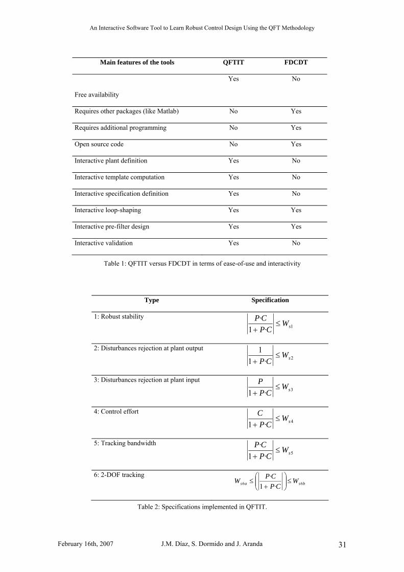
Table 1 briefly compares both tools while highlighting the differences between them, mainly those

related to interactivity and ease-of-use.

Thus the main difference between both tools is interactivity. Other differences between both tools are that

FDCDT requires the installation of Matlab. It thus offers more flexibility than QFTIT, but it is also more

difficult to use. On the other hand, QFTIT is freely available (http://ctb.dia.uned.es/asig/qftit/) and can

run under Windows-or Mac, without requiring any kind of programming to build an example (only

mouse operations or text insertion in dialog boxes have to be performed); in this way, the effort is

focused on understanding the fundamental concepts of the QFT technique without writing a line of code,

allowing the user to analyse interactively the effect that the modification of any plant/controller parameter

has on the stability of the closed-loop system and performance specifications, without requiring the

planning of iterative simulations. Therefore with QFTIT the user is very quickly visually aware of the

effects of his/her actions during the design.

3.1 Advantages of QFTIT

The present version of QFTIT offers the user, amongst others, the chance of observing the changes

instantly when some form of modification takes place in the available interactive objects:

1) Variations produced in the templates when a change of the uncertainties of the different components

of the plant or in the value of the template calculation frequency.

2) Individual, grouped or intersected variation in the bounds as a result of the configuration of

specifications, i.e., by adding zeroes and poles to the different specifications.

3) The motion of the controller’s zeroes and poles over the complex plane and the variation of its

symbolic transfer function when the open loop transfer function is modified in the Nichols diagram.

4) The change of shape of the open loop transfer function in the Nichols diagram and the variation of

the expression of the controller’s transfer function when any movement, addition or suppression of its

zeroes or poles in the complex plane.

5) The changes that take place in the temporary representation of the manipulated variable and in the

controlled variable due to the variation of the nominal values of the different elements of the plant.



6) The changes that take place in the temporary representation of the manipulated variable and of the

controlled variable due to the introduction of a step perturbation in the input of the plant. The

magnitude and the occurrence instant of the perturbation is configured by the user by means of the

mouse.

Further possibilities offered by QFTIT are:

7) Display of the points used in the sketch of the open loop transfer function in the Nichols diagram

during the loop-shaping stage.

8) Display of the points used to sketch the maximum and minimum values of the closed loop transfer

function in the Bode magnitude diagram during the pre-filter design stage.

9) Display of the points used to sketch the most unfavourable case of the system’s characteristic function

in the Bode magnitude diagram subject to validation and dependent of the selected type of

specification. It is also possible to emphasise the points in the curve associated to the frequencies for

which there are corresponding specifications. This feature helps the user to assess if the specification

is being fulfilled. This display takes place during the validation stage.

3.2. Current limitations of QFTIT

Obviously, the present version of QFTIT has some limitations:

a) Analysis and design of SISO systems. One of the most important limitations of the tool is that it can

only work with continuous SISO systems whose plant P is expressed in real factored form as follows:

( ) ( )

( ) ( )∏∏

∏∏

==

==

−

++⋅+⋅

++⋅+⋅= b

qqqq

n

ll

N

a

jjjj

m

ii

s

spss

szseKsP

1

200

2

1

1

200

2

1

τ

··2

··2·)(

ωωδ

ωωδ (1)

Where K, τ, zi, δj, ω0j, pl, δq, ω0q are independent variables which can take the following uncertainty in

their value:



[ ] +− ℜℜ⊂∈ oKKK maxmin , (2)

[ ] +ℜ⊂∈ maxmin ,τττ (3)

[ ] mizzz iii ,...,1, maxmin =ℜ⊂∈ (4)

[ ] nlzpp lll ,...,1, maxmin =ℜ⊂∈ (5)

[ ] ajojjj ,....,1, maxmin =ℜℜ⊂∈ +−δδδ (6)

[ ] ajjjj ,...,1, max0min00 =ℜ⊂∈ +ωωω (7)

[ ] bqoqqq ,....,1, maxmin =ℜℜ⊂∈ +−δδδ (8)

[ ] bqqqq ,...,1, maxmin =ℜ⊂∈ +ωωω (9)

b) Templates calculation. QFTIT only implements the algorithm by Gutman, Baril and Neunman [26] for

the calculation of templates. The maximum number of templates NT which the tool can support in the

current version is 10.

c) Specifications. The number of specifications in the frequency domain is also restricted (see Table 2).

The types of specifications implemented in QFTIT are similar to the FDCDT specifications [22]. In Table

2, Wsi, i=1,...,6. represents either a transform function or a vector where each of the elements is a certain

value expressed in decibels for a given frequency.

4. DESCRIPTION OF THE QFTIT INTERACTIVE TOOL

In this section in first place there is a description of the layout of the tool followed by a description, using

a design example, of the different elements displayed by the tool and the interactivity related to the

design stage. Finally there is a brief description of the Settings menu of the tool. A more detailed

description of QFTIT with several examples of robust control design using QFT methodology may be

obtained from the tools user guide available at http://ctb.dia.uned.es/asig/qftit/



4.1. Tool layout

QFTIT implements the QFT design methodology by considering a maximum of five design stages:

1) Templates computation. During this stage, the user defines the plant (1), by configuring the

uncertainty of its components. Furthermore, the user also selects the set of trial frequencies Ω.

{ } TN NN ≤=Ω ωωω ,...,, 21 (10)

The templates T(ωi) ωi ∈Ω are simultaneously computed and showed while user does these actions.

2) Specifications. In this stage, the user selects and configures the specifications (see Table 2) that

his/her design must fulfil. Each selected specification must configure the value of its associated W(s)

and select the frequencies under which each specification must be verified. There is also a

simultaneous generation, of associated bounds for each specification.

3) Loop-shaping. During this stage, the user performs the synthesis of the controller C(s) by shaping the

open loop transfer function L0(s) in the Nichols diagram.

4) Pre-filter design. In this stage the user performs the synthesis of the pre-filter F(s) if the Type 6

2-DOF tracking specification has been previously activated by shaping of the minimum and

maximum values of the closed loop transfer function in the Bode magnitude diagram.

5) Validation. In this stage the user makes sure that the specifications of his/her design are fulfilled.

When the user is working in a certain stage of the design, it is possible to advance on to the next stage or

return to any of the previous stages. Figure 2 shows these state transitions.



4.2 Description of the design stages: items and interactivity

The description of the different types of items displayed by the tool as well as the interaction amongst

them depending on the design stage will be done by means of an illustrative design example. A variation

of one of the robust control problems proposed in [20]. Let the family of plants:

P = [ ] [ ]⎭⎬⎫

⎩⎨⎧

∈∈+⋅

= 10,1,10,1)(

)( aKass

KsP (11)

Considering the nominal values Knom =9 and anom=8. The specifications that the system must fulfil are:

a) Type 1:Robust Stability. The desired phase margin is PM≥ 49.25º. An equation that relates PM with

Ws1 is given in [18]:

⎟⎟⎠

⎞⎜⎜⎝

⎛−−= 15.0acosº180º180 2

1sWPM

π º (12)

Clearing the previous expression yields Ws1=1.2 ∀ω≥0.

b) Type 6: 2-DOF tracking.

]15,0[10)4)(s3)(ss(

120)( (4.44) 4·s2·0.45·4.4 s

30) 0.7·(s )( 6226 ∈∀+++

=++

+= ωsWsW bsas

(13)

The set of trial frequencies considered is:

{ }100 15, 2, 1, 0.5, 0.1,=Ω (14)

The robust control problem consists in designing an adequate controller C(s) and pre-filter F(s) in order

for the closed loop system fulfilled the specifications.



4.2.1 Stage 1: Templates computation

In this stage of the design the display of the tool (see Figure 3) shows seven distinct areas: QFT design

steps, Options plot, Template frequency vector, Uncertainty plant description, Operations over plant P,

Templates and Status bar.

In the QFT design steps area the user has access to radio buttons which are associated to every previous

design stage, the present stage and the next stage. The present design stage is characterised by the

activation of its associated radio button. The user can select in the Options plot area different graphic

options associated to the figures shown in the windows such as the scaling types (automatic or fix) and

the type of line (solid or circle).

In the Template frequency vector area the user may configure the frequencies for the calculation of the

templates. There is a horizontal axis ω representing radians per seconds. It is possible to add, remove and

change the frequencies of the trial set Ω. Each of these frequencies is represented by a vertical segment

with an associated colour code which can be moved along the ω axis. For the proposed example six

frequencies must be added according to (14).

The Operations over plant P area is used to select the type of element of the plant (real-pole, real-zero,

complex-pole, complex-zero, integrator) on which we want to perform some type of action (move, add or

remove) in the Uncertainty Plant description area. It is also possible to configure it by using two sliders:

the uncertainty of the delay and the uncertainty of the gain of the plant, i.e., the specification of the

minimum, maximum and nominal values. For the proposed example the slider associated to the gain of

the plant would have to be moved in order to configure its minimum value kmin= 1, its maximum value

kmax=10 and its nominal value knom=9 .

The Uncertainty plant description area is used to graphically design the configuration of the uncertainties

of the poles and zeroes of the plant. This operation is carried out with the use of the mouse over the

selected pole or zero element. Figure 4 shows an example of how the uncertainty is represented for the



different types of possible elements of a plant. For the case of simple zeroes or poles the uncertainty is

represented by a segment whilst in the case of complex zeroes and poles it is represented by circular

sector limited by the maximum and minimum values of the damping factor and of the natural frequency

of each complex item (pole or zero). Both representations include the extreme values as well as the

nominal value.

In the proposed example, the elements of the plant (11) are the gain, which has already been configured

in the Operations over plant P area, an integrator and a simple pole with includes uncertainty. By

selecting the adequate options in the Operations over plant P area, it would be possible to add in the

Uncertainty plant description area an integrator and to configure by dragging the mouse the uncertainty

of the real pole a∈[1,10] and its nominal value anom=8. Figure 3 shows the final configuration of this area

for the proposed example.

The Templates area shows a Nichols diagram that includes the calculated templates T(ωi) ∈ Ω. For the

given example, Figure 3 shows in the Templates area six templates according to (14). The templates are

instantly recalculated each time one of the following items is changed:

a) The uncertainty of the zeroes and poles of the plant in Uncertainty plant description.

b) The gain of the plant in Operations over plant P.

c) The set Ω in Template frequency vector.

The Status bar area displays different types of messages and information depending on the position of the

mouse pointer within the window. For example, if the mouse pointer were to be situated over an item of

the plant in Uncertainty plant description zone, the maximum, minimum and nominal value would be

displayed in the Status bar.

4.2.2 Stage 2: Specifications



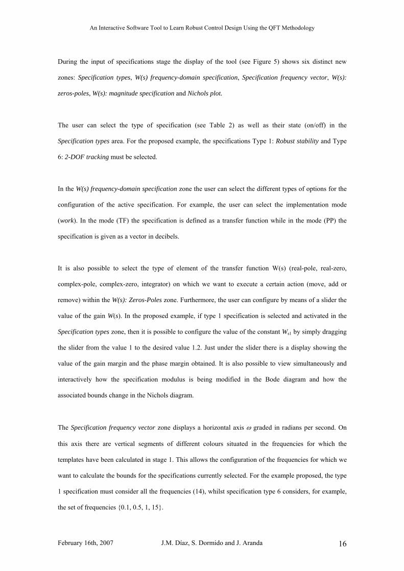
During the input of specifications stage the display of the tool (see Figure 5) shows six distinct new

zones: Specification types, W(s) frequency-domain specification, Specification frequency vector, W(s):

zeros-poles, W(s): magnitude specification and Nichols plot.

The user can select the type of specification (see Table 2) as well as their state (on/off) in the

Specification types area. For the proposed example, the specifications Type 1: Robust stability and Type

6: 2-DOF tracking must be selected.

In the W(s) frequency-domain specification zone the user can select the different types of options for the

configuration of the active specification. For example, the user can select the implementation mode

(work). In the mode (TF) the specification is defined as a transfer function while in the mode (PP) the

specification is given as a vector in decibels.

It is also possible to select the type of element of the transfer function W(s) (real-pole, real-zero,

complex-pole, complex-zero, integrator) on which we want to execute a certain action (move, add or

remove) within the W(s): Zeros-Poles zone. Furthermore, the user can configure by means of a slider the

value of the gain W(s). In the proposed example, if type 1 specification is selected and activated in the

Specification types zone, then it is possible to configure the value of the constant Ws1 by simply dragging

the slider from the value 1 to the desired value 1.2. Just under the slider there is a display showing the

value of the gain margin and the phase margin obtained. It is also possible to view simultaneously and

interactively how the specification modulus is being modified in the Bode diagram and how the

associated bounds change in the Nichols diagram.

The Specification frequency vector zone displays a horizontal axis ω graded in radians per second. On

this axis there are vertical segments of different colours situated in the frequencies for which the

templates have been calculated in stage 1. This allows the configuration of the frequencies for which we

want to calculate the bounds for the specifications currently selected. For the example proposed, the type

1 specification must consider all the frequencies (14), whilst specification type 6 considers, for example,

the set of frequencies {0.1, 0.5, 1, 15}.



The W(s): Zeros Poles zone displays a map of poles and zeroes that allows a configuration by means

changing the value with the mouse of the transfer function W(s) associated to a certain specification. It is

possible to add, move and suppress the zeros and the poles of W(s). As the transfer function W(s)

associated to the specification is configured, it is possible to view simultaneously and interactively in the

window how the modulus changes in the Bode diagram and how the bounds associated to the

aforementioned specification also changes in the Nichols diagram. For the proposed example, it would be

necessary to configure the transfer functions associated to the type 6 specifications in this specific zone.

In the case of Ws6a it would be necessary to configure a simple zero in –30, a pair of natural frequency

conjugated complex poles ω0=4.44 (rad/s) and dampening factor δ=0.45. On the other hand, for the case

of Ws6b it would be necessary to configure three simple poles in -3, -4 and -10. The gains of the transfer

functions would be configured in the W(s) frequency-domain specification zone

The modulus of the specification W(s) selected is represented in a Bode magnitude diagram in the W(s):

Magnitude specification zone. The contents of this graph are updated simultaneously and interactively

when the gain, zeros and poles of the specification W(s) change. For the proposed example, Figure 5

shows in this zone Ws6a(s) and Ws6b(s). Also shown the trial frequencies for Ws6a(s) (triangles) and for

Ws6b(s) (circles).

The Nichols Plot zone displays the bounds associated to the selected specification, the entire set of

bounds of the active specifications or the intersection of the bounds. Figure 5 shows in this zone how the

Nichols diagram represents the bounds associated to the type 6 specification once configuration has taken

place.

4.2.3 Stage 3: Loop-shaping

The display of the tool corresponding to the loop-shaping stage shows (see Figure 6) two new zones:

Operations over controller C and C(s): zeros -poles. In the first zone the user can select the type of item

(gain, real-pole, real-zero, complex-pole or complex-zero) associated to the controller C(s) subject to



input or manipulation in the zones C(s): Zeros-Poles and Nichols Plot. Also available is a slider by means

of which it is possible to configure the value of the gain of the controller.

In the C(s): Zeros-Poles zone it is possible to modify by dragging the object that represent the zeroes (o)

and poles (x) of the controller C(s). It is also possible to view the zeroes and poles of the nominal plant.

The actions carried out in this zone are reflected immediately in an interactive way in the representation

of the nominal open loop transfer function L0(jω) in the Nichols diagram as well as the symbolic

representation of the transfer function C(s).

During the design stage and in the Nichols Plot, further to the graphical representation of the final bounds

B(ωi) ωi ∈Ω associated to the specifications the function L0(jω) is also represented. The main

manipulation that the user can perform within this area of the programme is the displacement of L0(jω) in

certain directions in the Nichols diagram depending on the selected controller item in the Operations

Over Controller C zone.

The changes made to L0(jω) in the Nichols diagram are immediately reflected in an interactive way on the

zeroes-poles map corresponding to C(s) as well as in the symbolic expression of the transfer function

which appears under the Nichols Plot zone Likewise, the interactions performed by the user on the

zeroes-poles map of the controller will be reflected in the Nichols diagram. Thus, the user has a very

interactive and flexible tool to perform the synthesis of the controller. For the proposed example, Figure 6

displays the aspect of the QFTIT window after finishing the Loop-Shaping stage. The Nichols diagram

shows the bounds B(ωi) ωi ∈ Ω and the designed L0(jω). It can be observed how each point L0(jωi)

(circle) fulfil the boundary B(ωi). The expression of the designed controller is

(253.1) 1·s2·0.6·253. s 5) (s604541.66· )( 22 ++

+=sC (15)



This is a controller with a simple zero and a pair of conjugate complex poles which are represented in the

C(s): Zeros-Poles zone.

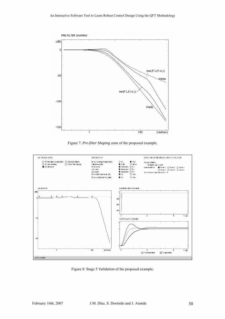
4. 2.4 Stage 4: Pre-Filter design

The zones of this stage and their interaction are very similar to the previous stage. Instead of the Nichols

plot zone appears Pre-Filter Shaping. In this zone the maximum and minimum values of the closed loop

transfer function F(s)·[L(s)/(1+L(s))] and the specifications W6a(s) and W6b(s) are represented in a Bode

magnitude diagram. The main manipulation that the user can perform within this area of the programme

is the displacement of the maximum and minimum values of F(s)·[L(s)/(1+L(s))] in certain directions in

the Nichols diagram depending on the selected F(s) item. Figure 7 shows the Pre-filter shaping zone at

the end of stage 4 for the proposed example. The display shows how the pre-filter

(4.4) s2·0.7·4.4· s 78.0) 0.25·(s )( 22 ++

+=sF (16)

made up of a single zero and a conjugate complex pole has been able to adjust the maximum and

minimum values of the closed loop transfer function F(s)·[L(s)/(1+L(s))] within the defined specifications

in (13).

4.2.5 Stage 5: Validation

The display of the tool corresponding to the Validation stage shows (see Figure 8) four new zones:

Selection of the specification to validate, Validation, Manipulated variable and Controlled variable. It is

also possible to show another additional zone: System: Zeros-Poles.

In the Selection of the specification to validate zone the user can select the chosen specification to be

validated. The Validation zone displays Bode magnitude diagram, which includes, depending on the

selected Type i specification, the modulus of its Wi(s) and the worst case modulus of the characteristic

function of the system (see Table 2) which is to validated. For the proposed example, Figure 8 displays a

horizontal line situated at 1.6 dB which is the representation of the robust stability specification Ws1=1.2.



Also displayed is the maximum value of the closed loop transfer function without considering the pre-

filter max{|L(jω)/(1+L(jω)|}. As max{|L(jω)/(1+ L(jω)|} does not surpass the horizontal line in any of the

frequencies the robust stability specification would be correct with the controller C designed during stage

3. With respect to the other specification established for this example. If the Type 6 specification is

selected for validation, the same figure that appears in stage 4 in the Pre-Filter shaping (see Figure 7)

appears now in the Validation zone, showing that with the designed pre-filter, the specification is

fulfilled.

The Manipulated Variable and Controlled variable zones show the manipulated variable u(t) and the

controlled variable y(t), respectively. It is possible to view the values of these variables for the case of the

non-compensated closed loop system (F=1, C=1) and/or for the case of a compensated closed loop

system. For the proposed example, Figure 8 shows the outputs of u(t) and y(t). Also displayed are the

upper level and the lower since the Type 6 specification was established in the controlled variable figure.

The user’s option regarding manipulation in this zone consists on the configuration of a manipulated

variable regarding the instant and the magnitude of a step type perturbation. This figure as well as the

controlled variable figure show simultaneously how this perturbation affects these variables.

The System: Zeros-Poles zone allows the display of a complex plane with the zeroes and poles of the

plant (including uncertainties), the controller, the pre-filter and the closed loop system. It is possible to

manipulated the nominal value of the plant’s zeroes and poles. Simultaneously and interactively the

display of the manipulated and controlled variables would be updated.

4.3 Settings menu

The QFTIT tool has a Settings menu that includes a total of thirty entries divided in nine groups. When

the user selects any of these entries a dialog box is displayed which includes a number of blank fields to

be completed. By doing so it is possible to perform the majority of the actions that could be performed by

only using the mouse as well as other additional functions, for example data input/output operations with

the tool.



5. EDUCATIONAL APLICATION OF QFTIT

QFTIT can be used with practical purposes to solve robust control problems, or with educational

purposes to teach the QFT methodology. From an educational point of view, the ease of use and

interactive nature of QFTIT are very useful for professors and students.

Professors can use QFTIT to illustrate their in-class QFT methodology explanations, and to make

laboratory work or homework for the students. Doing with QFTIT the tasks proposed by the professor,

students can intuitively learn QFT.

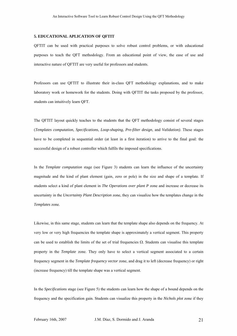
The QFTIT layout quickly teaches to the students that the QFT methodology consist of several stages

(Templates computation, Specifications, Loop-shaping, Pre-filter design, and Validation). These stages

have to be completed in sequential order (at least in a first iteration) to arrive to the final goal: the

successful design of a robust controller which fulfils the imposed specifications.

In the Template computation stage (see Figure 3) students can learn the influence of the uncertainty

magnitude and the kind of plant element (gain, zero or pole) in the size and shape of a template. If

students select a kind of plant element in The Operations over plant P zone and increase or decrease its

uncertainty in the Uncertainty Plant Description zone, they can visualize how the templates change in the

Templates zone.

Likewise, in this same stage, students can learn that the template shape also depends on the frequency. At

very low or very high frequencies the template shape is approximately a vertical segment. This property

can be used to establish the limits of the set of trial frequencies Ω. Students can visualise this template

property in the Template zone. They only have to select a vertical segment associated to a certain

frequency segment in the Template frequency vector zone, and drag it to left (decrease frequency) or right

(increase frequency) till the template shape was a vertical segment.

In the Specifications stage (see Figure 5) the students can learn how the shape of a bound depends on the

frequency and the specification gain. Students can visualize this property in the Nichols plot zone if they



drag the Kw slider in the W(s) frequency-domain specifications zone. The Nichols Plot zone shows the

bounds associated to the specifications in different colours. Each colour is associated to a certain

frequency. This feature helps students to distinguish the bounds.

Another idea that students can learn in this stage is that certain specifications can not be simultaneously

fulfil. If the Intersection option in the Options plot zone is selected then the Nichols Plot zone shows the

intersection of all the bounds associated to each established specification. If an intersection can not be

done at a certain frequency then QFTIT shows a message in the window to warn that it is not possible to

simultaneously fulfil all the specification established at such frequency. In this case, some of the

specifications must be relaxed or eliminated.

In the Loop-shaping stage (see Figure 6) students can quickly learn how a controller element (gain,

simple zero, simple pole, complex zeroes or complex poles) modifies the open-loop transfer function

L0(s) in the Nichols chart. Students only have to select a kind of element and the Add operation in the

Operations over controller C zone, place the mouse over L0, and drag it. The L0 shape is instantaneously

modified if the dragging is feasible with the kind of element. The QFTIT interactivity in this stage helps

students to gain skill in the synthesis of the controller G.

Besides, QFTIT interactivity also allows students to learn in the Pre-filter shaping stage how a pre-filter

element modifies the closed-loop transfer function T.

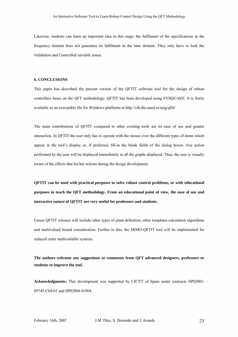
In the Validation stage (see Figure 8), students can determinate the frequencies where a specification is

not fulfilled. They only have to place the mouse over the characteristic function of the system (see Table

2) which is validated at the frequency where this fact occurs. The value of the frequency is displayed in

the Status bar.



Likewise, students can learn an important idea in this stage: the fulfilment of the specifications in the

frequency domain does not guarantee its fulfilment in the time domain. They only have to look the

Validation and Controlled variable zones.

6. CONCLUSIONS

This paper has described the present version of the QFTIT software tool for the design of robust

controllers bases on the QFT methodology. QFTIT has been developed using SYSQUAKE. It is freely

available as an executable file for Windows platforms at http://ctb.dia.uned.es/asig/qftit/

The main contributions of QFTIT compared to other existing tools are its ease of use and greater

interaction. In QFTIT the user only has to operate with the mouse over the different types of items which

appear in the tool’s display or, if preferred, fill-in the blank fields of the dialog boxes. Any action

performed by the user will be displayed immediately in all the graphs displayed. Thus, the user is visually

aware of the effects that his/her actions during the design development.

QFTIT can be used with practical purposes to solve robust control problems, or with educational

purposes to teach the QFT methodology. From an educational point of view, the ease of use and

interactive nature of QFTIT are very useful for professors and students.

Future QFTIT releases will include other types of plant definition, other templates calculation algorithms

and multivalued bound consideration. Further to this, the MIMO-QFTIT tool will be implemented for

reduced order multivariable systems.

The authors welcome any suggestions or comments from QFT advanced designers, professors or

students to improve the tool.

Acknowledgments: This development was supported by CICYT of Spain under contracts DPI2003-

09745-C04-01 and DPI2004-01804.



REFERENCES

1. B. Wittenmark, H. Häglund, and M. Johansson. Dynamic pictures and interactive learning. IEEE

Control Systems Magazine; 18(3), 26-32, (1998)

2. M. Johansson, M. Gäfvert, and K. J.Åström. Interactive tools for education in automatic control. IEEE

Control Systems Magazine, 18(3), 33-40, (1998).

3. Y. Piguet, U. Holmberg, and R. Longchamp. Instantaneous performance visualization for graphical

control design methods 1999, Proceedings of 14th IFAC World Congress, Beijing, China.

4. Y Piguet. SysQuake: User Manual. Calerga, (1999).

5. F. Esquembre. Easy Java Simulation: a software tool to create scientific simulations in Java.

Computer Physics Communications, 156, 199-204, (2004)

6. J. Sánchez, F.Esquembre, C.Martin, S.Dormido, S.Dormido-Canto, R.D.Canto, R.Pastor and

A.Urquia. Easy Java Simulations: an Open Source Tool for Develop Interactive Virtual Laboratories

using MATLAB/Simulink. The International Journal of Engineering Education 21(5), 798-813, (2005)

7. S. Dormido. Control learning: Present and future. Annual Reviews in Control, 28: 115-136, (2004).

8. S. Dormido, F. Gordillo, S. Dormido Canto S, and J. Aracil. An interactive tool for introductory

nonlinear control systems education. Proceedings of IFAC World Congress b’02 2002, Barcelona

(Spain).

9. S. Dormido. The role of interactivity in control learning (Plenary Lecture). Proceedings of the 6th



IFAC Symposium on Advances in Control Education ACE’03, Oulu (Findland). 2003, 1-12.

10. S. G. Crutchfield and W. J. Rugh. Interactive learning for signal, systems, and control. IEEE Control

Systems Magazine, 18(4), 88-91, (1998)

11. K. J. Åström, The future of control. Modeling, Identification and Control. 15(3), 127-134 (1994).

12. K. J. Åström, Limitations on control system performance. European Journal of Control;

6(1), 2–20, (2000).

13. I.M. Horowitz. Synthesis of feedback systems. Academic Press: New York, (1963).

14.I. M. Horowitz. Quantitative feedback design theory (QFT). QFT Publishers 660 South Monaco

Dorkway Denver, Colorado, (1992).

15. I. M. Horowitz. Survey of Quantitative Feedback Theory (QFT). International Journal of Robust and

Non-linear Control; 11(10): 887-921, (2001)

16. C. H. Houpis, R.R. Sating, S. Rasmussen, and S. Sheldon. Quantitative Feedback theory technique

and applications. International Journal of Control, 59: 39-70, (1992).

17. C. H. Houpis, S. J. Rasmussen, and M. García-Sanz. Quantitative Feedback Theory: fundamentals

and applications. 2nd Edition, CRC Taylor & Francis: Boca Ralen, (2006)

18. O. Yaniv. Quantitative feedback design of linear and nonlinear control systems. Kluwer Academic

Publishers : Norwell, Massachusetts, (1999).

19. J.M Díaz, S. Dormido, and J. Aranda. Interactive computer-aided control design using quantitative



feedback theory: the problem of vertical movement stabilization on a high-speed ferry. International

Journal of Control, 78 (11): 793-805, (2005).

20. J. D. D’Azzo and C. Houpis. Feedback control systems analysis and synthesis. Prentice Hall, (1998).

21. M. Barreras, P. Vital, M. García-Sanz, Interactive tool for easy robust control design. Proocedings of

the IFAC Internet Based Control Education 2001, Madrid (Spain), 83-88.

22. C. Borghesani, Y. Chait, and O. Yaniv, Quantitative Feedback Theory Toolbox - for use with

MATLAB. The MathWorks Inc, Natick, MA, (1995).

23. P. O. Gutman. Qsym User’s Guide and Reference Guide. Technion Israel Institute of Technology,

(1999).

24. C. H. Houpis and R. R. Sating RR. MIMO QFT CAD package (version 3). International journal of

robust and nonlinear control, 7: 533-549, (1997)

25. R. Nandakumar and G. D. Halikias. A new educational software tool for robust control design using

the QFT method. Proceedings of the 42nd IEEE Conference on Decision and Control 2003. Maui,

(Hawai USA), 803 -808.

26. P. O. Gutman, C. Baril, and L. Neumann. An algorithm for computing value sets of uncertain

transfer functions in factored real form. IEEE Transactions on Automatic Control; 29(6), 1268-1273,

(1995).



F C Pr e u

v d

y

n

-

H

Figure 1: Feedback System

STAGE 1

Templates computation

STAGE 2Specifications

STAGE 3Loop-shaping

STAGE 4Pre-filter design

STAGE 5Validation

Figure 2: Stage transitions in QFTIT.



Figure 3: Stage 1 Templates computation of the proposed example.

Figure 4: Uncertainty of the elements of the plant in QFTIT



Figure 5: Stage 2 Specifications of the proposed example.

Figure 6: Stage 3 Loop-shaping of the proposed example.



Figure 7: Pre-filter Shaping zone of the proposed example.

Figure 8: Stage 5 Validation of the proposed example.



Main features of the tools QFTIT FDCDT

Free availability

Yes No

Requires other packages (like Matlab) No Yes

Requires additional programming No Yes

Open source code No Yes

Interactive plant definition Yes No

Interactive template computation Yes No

Interactive specification definition Yes No

Interactive loop-shaping Yes Yes

Interactive pre-filter design Yes Yes

Interactive validation Yes No

Table 1: QFTIT versus FDCDT in terms of ease-of-use and interactivity

Type Specification

1: Robust stability 1·1

·sW

CPCP

≤+

2: Disturbances rejection at plant output 2·1

1sW

CP≤

+

3: Disturbances rejection at plant input 3·1 sW

CPP

≤+

4: Control effort 4·1 sW

CPC

≤+

5: Tracking bandwidth 5·1

·sW

CPCP

≤+

6: 2-DOF tracking bsas W

CPCPW 66 ·1·

≤⎟⎟⎠

⎞⎜⎜⎝

⎛+

≤

Table 2: Specifications implemented in QFTIT.

AN INTERACTIVE SOFTWARE TOOL TO LEARN ROBUST …€¦ · An Interactive Software Tool to Learn...

Documents

Transcript of AN INTERACTIVE SOFTWARE TOOL TO LEARN ROBUST …€¦ · An Interactive Software Tool to Learn...