An interactive real-time physics software for structural ...
118
Cover An interactive real-time physics software for structural analysis of space trusses Reydleon Paiva de Paulo Thesis to obtain the Master of Science Degree in Civil Engineering Supervisors: Prof. Dr. Vítor Manuel Azevedo Leitão Prof. Dr. Francisco Afonso Severino Regateiro Examination Committee Chairperson: Prof. Dr. António Manuel Figueiredo Pinto da Costa Supervisor: Prof. Dr. Vítor Manuel Azevedo Leitão Member of the Committee: Prof. Dr. José Paulo Moitinho de Almeida Sept 2020
Transcript of An interactive real-time physics software for structural ...

Cover
An interactive real-time physics software for
structural analysis of space trusses
Reydleon Paiva de Paulo
Thesis to obtain the Master of Science Degree in
Civil Engineering
Supervisors:
Prof. Dr. Vítor Manuel Azevedo Leitão
Prof. Dr. Francisco Afonso Severino Regateiro
Examination Committee
Chairperson: Prof. Dr. António Manuel Figueiredo Pinto da Costa
Supervisor: Prof. Dr. Vítor Manuel Azevedo Leitão
Member of the Committee: Prof. Dr. José Paulo Moitinho de Almeida
Sept 2020

Declaration
I declare that this document is an original work of my own authorship and that it fulfills all the
requirements of the Code of Conduct and Good Practices of the Universidade de Lisboa.

i
“FAOT – Facilitar, Alterar, Otimizar e Transformar” Reydleon Paulo 2014

ii

iii
Agradecimentos
Aos meus orientadores, Professor Vítor Leitão e Professor Francisco Regateiro, pela ajuda na
resolução de problemas ao longo das várias etapas deste trabalho, pelas suas correções e sugestões.
Agradeço a atenção que tiveram comigo durante este ano em que tive o privilégio de receber uma bolsa
de estudos "Eng. Augusto Ramalho-Rosa". A importância de uma bolsa de estudos na vida de um
estudante como eu é inexplicável e imensurável. Hoje e ao longo da minha vida sempre serei um
bolseiro agradecido à Dra. Berta Marinho, Dra. Rita Schreck e ao Eng. Augusto Ramalho-Rosa.
Agradeço também a atenção que me foi dada por todos os profissionais dos SAS Ulisboa e do NDA,
em particular ao Dr. José Barbosa e à Dra. Rita Wahl.
Agradeço a todos os meus amigos, em particular, ao Eng. Eduardo Lopes, à Sofia Alves, ao Eng. Andrei
Vodã e ao Eng. Bruno Alexandre Morais Ribeiro. Um especial agradecimento à Engenheira Ana Beatriz
Rodrigues e à sua família: José Ambrósio, José Miguel e Graciete Novais.
Agradeço à minha mãe, Derli, e aos meus irmãos Gabryel e Simão Paulo pelo apoio e por estarem
sempre do meu lado. Dedico esta dissertação à minha mãe por me encorajar e que, em fases decisivas
da minha vida, me tem apoiado e esclarecido como nenhuma outra pessoa.

iv

v
Abstract
Space truss is an important theme while learning the first concepts of statics. On the other hand, it has
real engineering applications. An example of the application of this technique is the Double Layer Grid
(DLG), which is generally the adopted solution in the roofing of factories and airport terminal halls, as it
can overcome large spans.
This work presents an interactive software entirely written in Python that aims to help students to
understand the behavior of space truss systems. The software allows the user to design structures,
analyze them, and then export the results. The CAD software was successfully created from scratch
and can perform nonlinear analysis.
The 3DParticleSystem software numerical method is based on the concept of physics engine. Physics
engines are widely used as middleware in game engines. In commercial software for structural analysis,
this approach is rarely used despite exhibiting some quite convenient features: it allows for new types
of analysis (namely, nonlinear and incremental analysis); also allowing to represent the time evolution
of a structure once calculations are made in real-time, responding to user input. Such features can be
important while learning structural engineering concepts.
The work carried out here further improves the application of physics engines in the field of structural
analysis: it first summarizes the implementation of the physically-based modeling/particle system
dynamics; it then gives an overview of the PyQt and the Panda3D game engine, tools that were used
to create an advanced GUI (Graphical User Interface) to render space trusses.
Keywords: Interactive Structural Analysis, Python 3D physics engine, Panda3D, Nonlinear Analysis,
Newton's Second Law, Particle System Dynamics.

vi
Resumo
A treliça espacial é um tema importante ao aprender os primeiros conceitos de estática. Por outro lado,
esta tem aplicações reais em engenharia. Um exemplo da utilização desta técnica é o Double Layer
Grid (DLG). Esta técnica é geralmente adotada em coberturas de fábricas e terminais de aeroporto,
pois pode superar vãos grandes.
Este documento apresenta um software interativo inteiramente escrito em Python que visa ajudar os
alunos a compreender o comportamento de treliças espaciais. O software permite criar estruturas,
analisá-las, em seguida, exportar os resultados. Este CAD foi criado de raiz e é capaz de realizar
análises não-lineares.
O método numérico do 3DParticleSystem software é baseado no conceito de physics engine. Physics
engine é uma abordagem normalmente utilizada em game engines. Porém, não tanto na área de
engenharia de estruturas. Sendo assim, não é a abordagem mais comum em software comerciais para
a análise de estruturas. A grande vantagem desta abordagem é que permite complexos tipos de
análises, tais como, análises não-lineares e incrementais. Além disso, permite representar a evolução
temporal de uma estrutura uma vez que os cálculos são feitos em tempo real. Tais vantagens podem
ser cruciais na aprendizagem de conceitos de engenharia de estruturas.
Este documento contribui numericamente na aplicação de physics engines na análise de estruturas.
Primeiramente, apresenta a implementação da metodologia physically based modeling/particle system
dynamics. Além disso, dá uma visão global do PyQt e do Panda3D, ferramentas utilizadas para
desenvolver a GUI (Graphical User Interface) capaz de representar treliças espaciais.
Palavras-chave: Análise estrutural interativa, Python 3D physics engine, Panda3D, Análise não linear,
Segunda Lei de Newton, Particle System Dynamics.

vii
Notation
𝑎 Acceleration vector [ms−2]
𝐴 Cross-sectional area [m2]
c Damping coefficient [kNm−1s]
𝜌 Density [ms−2]
𝐹 𝑜𝑟 𝑓 Generic force [kN]
𝐿 Length [m]
𝑚 Mass [kg]
𝜆 Mass per unit length [kgm−1]
𝛥𝑡 time-step [s]
𝑘 Stiffness [kNm−1]
𝜖 Strain [−]
σ Stress [MPa]
𝑡 time [s]
𝑣 Velocity vector [ms−1]
E Young’s modulus [GPa]

viii
Acronyms
CSV Comma-separated values
CAD Computer-aided design
DLG Double Layer Grid
𝐷𝑋𝐹 Drawing Exchange Format
FEM Finite Element Method
FPM Finite Particle Method
GE Game engine
GRE Graphics rendering engine
GUI Graphical user interface
PS Particle System approach
𝑃𝐸 Physics engine
TXT Text file
VFIFE Vector Form Intrinsic Finite Element method

ix
Contents
1 Introduction 1
1.1 Motivation 1
1.2 Physics engine and Game engine 2
1.2.1 Physics engine 2
1.2.2 Game engine 3
1.3 Real-time physics software in structural engineering 3
1.4 Particle-based methods in structural engineering 4
1.4.1 Vector Form Intrinsic Finite Element method 4
1.4.2 Finite Particle Method 5
1.5 Overview and objectives 7
1.6 Document outline 9
2 Particle System Approach 3D (The Physics Engine) 11
2.1 Mechanical behavior of materials 11
2.1.1 Stress and strain 11
2.1.2 Elastic behavior 13
2.1.3 Elastic-plastic behavior 13
2.2 Particle System Dynamics 14
2.2.1 Newton's second law 15
2.2.2 Particle definition and particle mass 16
2.2.3 Local deformation coordinate system of a space rod element 16
2.2.4 Calculation of the internal nodal forces 17
2.2.5 Convergence and stability 20
2.3 Numerical implementation of the PSA3D physics engine 23
2.3.1 Numerical method 23
2.3.2 Numerical process – Approach 1 24
2.3.3 Numerical process – Approach 2 27
2.4 Stopping criterion 29
3 The 3DParticleSystem Software 31
3.1 The 3DParticleSystem GUI 31
3.1.1 Units 31
3.1.2 Camera control 32
3.1.3 The 3DParticleSystem GUI overview 32
3.2 Software structure 38
3.2.1 Python and Anaconda 38

x
3.2.2 The 3DParticleSystem structure 38
3.2.3 Physics engine programming challenges 40
3.3 Qt framework and PyQt 40
3.4 Panda3D 40
3.4.1 Brief Panda3D description and basic features 40
3.4.2 ShowBase class 41
3.4.3 LineNodePath class 41
3.4.4 ElementaryLine, ElementaryArc and Arrow classes 42
3.4.5 GameEngine3DParticleSystem class 43
3.5 Elements 43
3.5.1 Particles 44
3.5.2 Rod 45
3.6 Simulation mode 46
4 Modeling 49
4.1 Relative difference 49
4.2 Numerical simulation – Approach 1 49
4.2.1 Axial force rod problem 49
4.2.2 7-bar plane truss 55
4.2.3 9-bar space truss 59
4.3 Numerical simulation – Approach 2 61
4.3.1 7-bar plane truss 61
4.3.2 24-bar Space Truss (shallow geodesic dome) 62
4.3.3 Double Layer Grid 65
4.4 Summary 67
4.5 Changing the model during the simulation 68
4.5.1 Removing rods in a statically indeterminate structure 68
4.5.2 Changing nodal constraints 69
4.5.3 Removing a rod in the 9-bar Space Truss 70
4.5.4 Analyzing a Double Layer Grid 71
5 Conclusions 73
5.1 Main conclusions 73
5.2 Directions for future work 73
5.2.1 Frame analysis 73
5.2.2 Numerical method 74
5.2.3 Nonlinearity 74
5.2.4 Programming improvements 74

xi
5.2.5 Usability 74
References 75
Annex A – Setting the 3DParticleSystem Software 81
A.1 Some installation notes 81
A.2 Setting the 3DParticleSystem software 82
A.2.1 Setting the input file 82
A.2.2 Setting the structural system file 83
Annex B – Parts of the 3DParticleSystem software code 84
B.1 The3DParticleSystem 84
B.2 The3DParticleSystemGUI 85
B.3 The3DPsDialog 85
B.4 GameEngine3DParticleSystem 86
B.4.1 GameEngine3DParticleSystem.__init__ (Class constructor) 86
B.4.2 GameEngine3DParticleSystem.__simulate__ (private method) 86
B.5 PSA3DElements 87
B.5.1 PSA3DElements.__initStructureSystem__ (private method) 87
B.5.2 PSA3DElements.__addParticle__ (private method) 87
B.5.3 PSA3DElements.__addRod__ (private method) 88
B.5.4 PSA3DElements.updateStructureSystem (public method) 88
B.6 PSA3DPhysicsEngine 89
B.6.1 PSA3DPhysicsEngine Numerical process 89
B.6.2 Approach 1 90
B.6.3 Approach 2 92
B.7 Graphics Rendering Engine 94
B.7.1 LineNodePath 94
B.7.2 ElementaryLine 95
B.7.3 GraphicsParticles 95
B.7.4 GraphicsRods 95
B.8 Utils functions 96
B.8.1 matrixOperations 96
B.8.2 TransformationFunctions 98

xii

xiii
List of Figures
Figure 1.1 – Pymunk and Pygame demonstration. Slide and pin joint [89]............................. 2
Figure 1.2 – Arcade (left side). PushMePullMe (right side). ................................................... 3
Figure 1.3 – Progressive deformation of a Vogel six-story frame with rigid connections,
adapted from [36]. ......................................................................................................... 5
Figure 1.4 – Progressive deformation of a Vogel six-story frame with linear semi-rigid
connections. Adapted from [36]. .................................................................................... 5
Figure 1.5 – Cantilever-framed structure: (a) structure in use (Image by Y. Yu); (b)
axisymmetric view; (c) plane view; (d) vertical view. Adapted from [6] ........................... 6
Figure 1.6 – Vertical view of cantilever structure failure process. Adapted from [6]. ............... 6
Figure 1.7 – FPM model of a planar frame. Adapted from [36]. ............................................. 7
Figure 1.8 – The 3DParticleSystem software Venn diagram. ................................................. 8
Figure 2.1 – Stress-strain curves. Typical ductile steel tensile test, on the left (adapted from
[90]). Compressive strength test, on the right (adapted from [91]). ................................12
Figure 2.2 – Symbolic one-dimensional models: (a) The elastic-perfectly plastic solid with the
yield limit Fy. (b) The elastic-plastic body with linear strain hardening. Adapted from [92].
.....................................................................................................................................14
Figure 2.3 – (a) space truss structure; (b) discretization of the structure by particles and
elements; (c) particles and forces. Adapted from [6]. ....................................................15
Figure 2.4 – Forces acting on a particle of a rigid space truss. Adapted from [30]. ...............15
Figure 2.5 – The local coordinate system of space rod – positive sign convention (left) and
negative sign convention (right). ...................................................................................16
Figure 2.6 – A simple rod element with its initial and current configuration. ..........................18
Figure 2.7 – (a) Reversed motion. (b) Forward motion. Adapted from [6]. ............................19
Figure 2.8 – The trace of a typical kinetic energy peak. Adapted from [93]. ..........................22
Figure 2.9 – Numerical method flow chart. ...........................................................................24
Figure 2.10 – Numerical process – Approach 1 flow chart. ...................................................24
Figure 2.11 – Numerical integration of the equation of motion – Trapezoidal rule flow chart. 26
Figure 2.12 – Flow chart for the calculation of rods’ axial forces in Approach 1. ...................26
Figure 2.13 – Numerical process – Approach 2. ...................................................................27
Figure 2.14 – Stage 1 of the Kinetic Damping approach - Numerical integration flow chart. .27
Figure 2.15 – Stage 2 of the Kinetic Damping approach – flow chart. ...................................28
Figure 2.16 – Flow chart for the calculation of rods’ axial forces in Approach 2. ...................29
Figure 3.1 – The 3DParticleSystem software menu. .............................................................33
Figure 3.2 – (a) space tower with a square base. (b) deformed shape with the original
structure in the back. (c) deformed shape. ....................................................................33

xiv
Figure 3.3 – Plane truss. Adapted from FTOOL....................................................................34
Figure 3.4 – Definition of particles and rods in the 3DParticleSystem software. ....................35
Figure 3.5 – An example of defining support constraints and external forces in the
3DParticleSystem software. ..........................................................................................35
Figure 3.6 – An example of defining the cross-sectional area and the material’s mechanical
properties in the 3DParticleSystem software.................................................................36
Figure 3.7 – The results of the particles in the 3DParticleSystem software. ..........................36
Figure 3.8 – The results of the rods in the 3DParticleSystem software. ................................37
Figure 3.9 – The results of stress and strain in the 3DParticleSystem software. ...................37
Figure 3.10 – Importing from AutoCAD 2018 to the 3DParticleSystem software. ..................37
Figure 3.11 – Communication among the user and different modules (GUI, GE, PE, and
GRE). ...........................................................................................................................39
Figure 3.12 – GUI window of Panda3D ShowBase. ..............................................................41
Figure 3.13 – Inheritance diagram for LineNodePath class. Adapted from [88]. ...................42
Figure 3.14 – Rendering an ElementaryLine object in a simple Panda3D application. ..........42
Figure 3.15 – Representation of lines, arrows, and circles in the 3DParticleSystem software.
.....................................................................................................................................43
Figure 3.16 – (a) plane truss structure; (b) discretization of the structure in particles and rods.
.....................................................................................................................................44
Figure 3.17 – Graphical representation of the particles, on the left, plane truss structure, on
the right. .......................................................................................................................44
Figure 3.18 – Different types of nodal constraints in the 3DParticleSystem software. From left
to right, ball joint in X0Y and Y0Z, roller along y and x, ball-and-socket joint. ................44
Figure 3.19 – Representation of external forces (left). Representation of a complete plane
truss with reaction support results (right). .....................................................................45
Figure 3.20 – The deformed and the original shape of a plane truss structure in the
3DParticleSystem software on the left. The deformed shape without the original shape
on the right. ..................................................................................................................46
Figure 3.21 – Axial force diagram of a plane truss structure in the 3DParticleSystem.
software. .......................................................................................................................46
Figure 4.1 – One-dimensional axially loaded rod problem, adapted from FTOOL. ................49
Figure 4.2 – Displacement at Particle B (Δt = 2x10⁻⁴ s and c = 200 kN ∙s/m). .......................50
Figure 4.3 – Nodal Forces in Particle B (Δt = 2x10⁻⁴ s and c = 200 kN ∙s/m). .......................51
Figure 4.4 – The deformed shape, amplified 100x (left). Stress-strain curve after 120
iterations (right). ............................................................................................................51
Figure 4.5 – Nodal Forces in Particle A (Δt = 2x10⁻⁴ s and c = 200 kN ∙s/m). .......................52
Figure 4.6 – Rod 1. Axial force (Δt = 2x10⁻⁴ s and c = 200 kN ∙s/m). ....................................52

xv
Figure 4.7 – Rod 1. Variation of the displacement with the stiffness. ....................................53
Figure 4.8 – Rod 1. Variation of the internal forces with the stiffness. ...................................53
Figure 4.9 – Rod 1. Damping force changing over the damping coefficient. time-step Δt =
2x10⁻⁴ s. ........................................................................................................................54
Figure 4.10 – Rod 1. Damping force changing over the damping coefficient. time-step Δt =
2.1x10⁻⁴ s. .....................................................................................................................54
Figure 4.11 – 7-bar plane truss problem (adapted from FTOOL). .........................................55
Figure 4.12 – Axial forces in the 7-bar plane truss problem. E A = 4 X 10⁵ kN. ....................56
Figure 4.13 – The deformed shape of the 7-bar plane truss, amplified 50x (left). Stress-strain
curve after 822 iterations (right). ...................................................................................57
Figure 4.14 – Rod 7. Axial Forces over the iterations. ..........................................................58
Figure 4.15 – Vertical relative displacement of Particle B over the iterations. .......................58
Figure 4.16 – 9-bar space truss. Adapted from [76]. .............................................................59
Figure 4.17 – 9-bar space truss. Axial forces. .......................................................................60
Figure 4.18 – 9-bar space truss. The deformed shape considering a scaling factor of 100. ..60
Figure 4.19 – 7-bar plane truss problem. E A = 4 X 10⁴ kN. .................................................61
Figure 4.20 – ASM International in Ohio, USA, [94] (left). Environment Museum in Montreal,
Canada, [95] (right). ......................................................................................................62
Figure 4.21 – 24-bar space truss (left). Axisymmetric view of the 24-bar space truss in the
3DParticleSystem software (right). ................................................................................63
Figure 4.22 – 24-bar space truss. The computed axial forces using the developed software
from a top view (left) and axisymmetric view (right). ......................................................64
Figure 4.23 – The deformed Shape. Lateral view (left). Axisymmetric view (right) ................64
Figure 4.24 – Double Layer Grid (DLG) analyzed by Vendrame. Axisymmetric view of the
DLG in the developed software. ....................................................................................65
Figure 4.25 – Double Layer Grid (DLG). Top view of the DLG showing the analyzed rods
(left). The deformed shape (right). ................................................................................66
Figure 4.26 – Axisymmetric view of DLG’s deformed shape in the 3DParticleSystem
software. .......................................................................................................................66
Figure 4.27 – Evolution of the structure system due to the removal of Rod 1. ......................69
Figure 4.28 – Axial forces for the resulting structure after removing Rod 1. ..........................69
Figure 4.29 – Static equilibrium situation of a 7-bar plane truss system. The deformed shape.
.....................................................................................................................................69
Figure 4.30 – Static equilibrium situation of a 7-bar plane truss system. Axial forces. ..........69
Figure 4.31 – Evolution of the system after changing the nodal constraint and removing a
rod. ...............................................................................................................................70

xvi
Figure 4.32 – Image sequence showing the collapse of 9-bar space truss when removing
Rod 9. The deformed shape scaled 100 times (right). ...................................................70
Figure 4.33 – DLG. After removing three zero-force members of the system .......................71
Figure 4.34 – Left to right. The label of the removed rods. DLG results after rods removal, top
view, and axisymmetric view. ........................................................................................71
Figure 4.35 – DLG mechanism after removing a fundamental rod. .......................................72

xvii
List of Tables
Table 3.1 – The units needed for the 3DParticleSystem software input. ...............................31
Table 3.2 – Default Panda3D’s camera control system. .......................................................32
Table 4.1 – Particles A and B, and their properties. ..............................................................50
Table 4.2 – Rod 1 and its properties. ....................................................................................50
Table 4.3 – Particles A and B, and their properties. ..............................................................55
Table 4.4 – Geometry and properties of the rods. .................................................................55
Table 4.5 – 7-bar plane truss. Axial forces. ...........................................................................56
Table 4.6 – Relative displacements in the 7-bar plane truss. ................................................57
Table 4.7 – 9-bar space truss. Axial forces. ..........................................................................59
Table 4.8 – 9-bar space truss. Relative displacements. ........................................................60
Table 4.9 – 7-bar plane truss. Axial forces. ...........................................................................61
Table 4.10 – 24-bar space truss. Stress and strain results. ..................................................62
Table 4.11 – Relative displacements in the 7-bar plane truss. ..............................................62
Table 4.12 – 24-bar space truss. Stress and strain results. ..................................................63
Table 4.13 – 24-bar space truss. Displacements results. ......................................................63
Table 4.14 – Double Layer Grid (DLG). Axial forces. ............................................................66
Table 4.15 – Double Layer Grid (DLG). Stress and strain results. ........................................67
Table 4.16 – Resume. Geometry and the respective number of iterations required to meet
the stopping criterion for several truss structures. .........................................................67
Table 4.17 – The total solution time for the simulation of the Double Layer Grid...................68

xviii

Page 1 of 98
1 Introduction
1.1 Motivation
As knowledge evolves, there is a natural increase in technical requirements for structural engineering
projects. Thus, software knowledge becomes essential when it comes to obtaining the best solution in
the shortest possible time. Therefore, this knowledge is fundamental at the professional level and should
be presented to the students during the academic period. Thus, several tools have been developed to
employ full numerical structural analysis and to handle structural phenomena, for example, commercial
programs such as ANSYS Inc. (2011) and SAP2000 (Computers and Structures Inc. 2011). These
programs, however, are designed for advanced users and are challenging to learn and use.
The analysis of trusses (structures composed of bars/rods connected at their ends by hinges and subject
to loads applied only at the nodes/hinges) is an important theme in learning the first concepts of
structural mechanics. The static equilibrium of plane (2D) trusses is generally presented in the first
semesters of engineering courses. During this stage, didactic software are usually introduced to support
learning the basics of structural engineering. Usually, these codes implement the linear static model and
the direct stiffness method [1]. This is suitable for academic purposes, but entails some limitations: if
the student attempts to model a structure that is hypostatic or if the configuration of supports in a model
does not render it externally isostatic, most of the didactic software will simply produce an error message
saying that the structure cannot be analyzed because it is an unstable structure [2]. Moreover, due to
its numerical simplifications, they are not suitable for teaching some topics, such as physical nonlinearity
and failure mechanisms, as they do not address these matters effectively or at all.
There are some numerical alternatives to the traditional Finite Element Method (FEM) that may be seen
to avoid some of the above difficulties. One such alternative resorts to particle-based methods. These
methods are widely used in the development of games and animations but also have applications in
structural engineering problems where methods have been devised for problems such as structural
form-finding problems [3], and others based on the dynamic relaxation method [4]. Unlike the methods
based on finite elements, there is no need to construct a global stiffness matrix and solve it [5]. Typically,
a particle-based approach is built on sets of particles that carry all the physical properties and conditions;
then, equilibrium is verified at each particle in an iterative process. This approach allows different
analyses to be carried out by simply enforcing Newton's laws at each particle, making it possible to
address kinematically indeterminate structures [1], discontinuities, failure mechanisms [6], and also
physically and geometrically nonlinear problems. For a student learning the basics of structural
engineering, the answer to some previous topics can be difficult to relate to the real world. Besides, it
takes time and experience to understand the behavior of structures. Thus, a software that allows real-
time physics interactive analyses can be a useful tool for an engineering student to start learning these
relevant engineering topics.

Page 2 of 98
1.2 Physics engine and Game engine
For the development of an interactive real-time physics software for structural analysis, there are several
possible approaches. The one favored here is to use concepts commonly used in computer games.
This thesis starts by describing two fundamental concepts: the physics engine and the game engine.
1.2.1 Physics engine
Physics engines are often described as game middleware that are integrated into a game engine to
handle some specialized aspects in physics simulation, such as collision detection and dynamics
simulation [7]. Physics engines are packages that provide specialized mechanical simulation and are
responsible for solving Newton's equation of motion. It handles certain physical systems such as rigid
body dynamics, soft body dynamics, fluid dynamics and collision detection. Havok [8], PhysX [9], Open
Dynamics Engine [10], and Chipmunk [11] are some of the most popular game-oriented physics
engines.
Some developer-friendly physics engines can be included in different applications, such as game
engines, digital content creation systems, and effects applications. An example of a developer-friendly
physics engine is Pymunk [12], which is built on top of the 2D physics library Chipmunk, for the Python
programming language [13]. This physics engine can handle rigid bodies, collision shapes, and
constraints/joints. In Figure 1.1, the Pymunk library is used to create an animation of randomly falling
balls over a rigid body, constrained by a slide and a pin joint. In this case, it is combined with PyGame
[14] as a graphics rendering middleware to render the simulation results.
In addition to video game applications, physics engines are widely used in physically-based animations
[15]. In the last decade, physics engines are also being used for robotic applications such as Mira –
Middleware for Robotic Applications [16] and MuJoCo – A physics engine for model-based control [17].
Figure 1.1 – Pymunk and Pygame demonstration. Slide and pin joint [89].

Page 3 of 98
1.2.2 Game engine
Game engines, all-in-one middleware, normally correspond to a Software Development Kit (SDK), which
integrates the functionalities needed to develop a game. These functionalities, also known as
middleware, can be graphics/rendering, audio, physics, Artificial Intelligence, multiplayer, synthesis,
among others [7]. Some popular commercial game engines with their representative games are
Renderware (Grand Theft Auto: San Andreas) [18], Unity (Assassin’s Creed: Identity) [19], and Unreal
(Borderlands) [20].
1.3 Real-time physics software in structural engineering
Real-time physics simulation has been extensively used in computer games, but its potential has yet to
be fully realized in design and education. It is suitable to simulate the behavior of structures under
different loading with engineering accuracy and giving real-time feedback [5]. Some didactic programs
aim to introduce the first structural engineering concepts and are directly related to the core of this thesis.
Of these, two programs stand out, namely, Arcade and PushMePullMe3D.
Arcade [21], created by Kirk Martini (latest release in 2009), is a structural analysis software program
for nonlinear dynamic simulation specially tailored for students and classes of architecture and structural
engineering courses. It is based on a computation method widely used in computer games to create an
interactive real-time linear and nonlinear physical simulation of simple structures.
PushMePullMe3D [22], which is part of the educational project Expedition Workshed, is written in Java
and is available online. It is based on the idea of using interactive real-time physics, where a co-rotational
approach is used to compute the resultant field of displacements in global coordinates, including the
effect of large deformations.
Figure 1.2 shows, on the left, the Arcade’s GUI, while analyzing an inelastic behavior of a cantilever; on
the right, the PushMePullMe3D’s GUI is shown while analyzing a space truss.
Figure 1.2 – Arcade (left side). PushMePullMe (right side).

Page 4 of 98
1.4 Particle-based methods in structural engineering
Particle-based methods have a real application in advanced civil engineering problems. In recent years,
some researchers have put effort into developing particle methods suitable for application to structural
analysis. Thus, this chapter provides an overview of two particle-based methods, the Vector Form
Intrinsic Finite Element method, VIFIFE, and the Finite Particle Method, FPM.
1.4.1 Vector Form Intrinsic Finite Element method
The Vector Form Intrinsic Finite Element method (VFIFE) is a mathematical calculation method based
on vector mechanics for structures with large deformation. The method appears to have been first
proposed by Ting, Wang, and Shi in 2002 and is based on an intrinsic modeling approach, an explicit
algorithm, and a co-rotational formulation of kinematic, meaning that it is a step-by-step and particle-by-
-particle cycling iteration computation that follows the motion of the particles.
In a series of three papers, Ting explains the fundamentals of the VFIFE method. In the first paper, the
author presents the basics of the method as applied to a plane frame element model [23]. In the second
work, the author introduces the formulation for plane solid elements and makes some remarks related
to convergence [24]. Finally, the author presents a convected material frame which is used to extend
the method for the large deformation and large displacement cases. Some interesting examples are
also presented, including the case of bending of a flexible cantilever with contact [25].
The VFIFE is based on some assumptions, which are:
a) the structural system is a finite collection of rigid and/or deformable bodies,
b) the motion of the bodies follows Newton's second law,
c) all the existing bodies must have mass,
d) each body mass is represented by a finite number of particles.
The VFIFE method can be applied to a broad spectrum of problems. For example, it was used to analyze
the snap-through of a space truss dome [26] as well as to simulate a 3D frame collapse [27]. With a
slightly different implementation, it was used to analyze the nonlinear behavior of steel structures
exposed to fire [28]. More recently, it has been used to analyze train and bridge dynamic interaction
responses [29].

Page 5 of 98
1.4.2 Finite Particle Method
The Finite Particle Method (FPM) is a numerical analysis method based on VFIFE that focuses more on
structural engineering. It was developed in 2008 by Ying Yu and Yao-Hi Luo and presented in two papers
[30] and [31] both in Chinese. Then, the principles of FPM are also described in English by Long et al.
in [32], which applied the method in the simulation of the collapse of a 3D space structure frame
subjected to earthquake excitation. A comparison with FEM results was also included in this last work.
The FPM has already shown its applicability in various types of problems, namely: analyzing
kinematically indeterminate bar assemblies [33] and deployable structures [34], making a progressive
failure simulation [6] and a collapse analysis of cable nets under dynamic loads [35]. Most recently, it
was used to analyze the nonlinear dynamic collapse analysis of semi-rigid steel frames [36]. The
following figures present the results of the progressive deformation of the Vogel six-story frame with
rigid connections, in Figure 1.3, and with linear semi-rigid connections, in Figure 1.4.
Figure 1.4 – Progressive deformation of a Vogel six-story frame with linear semi-rigid connections.
Adapted from [36].
Figure 1.3 – Progressive deformation of a Vogel six-story frame with rigid connections, adapted from
[36].

Page 6 of 98
One of the most interesting applications of FPM is the progressive failure simulation of truss structures
[6]. In this work, a cantilever-framed structure was analyzed to simulate the roof of an audience stand
at Sanmen in China that was destroyed by a typhoon in 2005. Figure 1.5 shows the roof modeled as a
cantilever truss structure. Each member of the structure was modeled by a 3D rod element and two
particles. The total numbers of particles and rod elements were 416 and 1456, respectively.
A typhoon is one of the most complicated types of dynamic loads. Because the focus of the work was
on the failure simulation algorithms, the wind loads were, for simplicity, taken as constant impact loads
in the analysis. Moreover, the deformations of the pillars were ignored in the analysis, and so fixed roof
supports were considered. The results of this analysis are shown in Figure 1.6.
Figure 1.5 – Cantilever-framed structure: (a) structure in use (Image by Y. Yu); (b) axisymmetric view;
(c) plane view; (d) vertical view. Adapted from [6]
Figure 1.6 – Vertical view of cantilever structure failure process. Adapted from [6].

Page 7 of 98
1.4.2.1 Particle definition
The bodies specified in the VFIFE method correspond in the Finite Particle Method to mass points, the
particles. The particles are connected by rods, and the motion of the particles follows Newton's second
law. The rod element, which has no mass, connects these particles with point values, and all internal
forces and external forces are added to the particles. Equilibrium is instead enforced on each particle,
resulting in the internal nodal force and external force being balanced continuously. Figure 1.7 presents
the FPM model of a planar frame [36].
1.4.2.2 Modeling material nonlinearity
The particle motion equation is the same for nonlinear materials and linear ones as well. Therefore, the
only difference between linear and nonlinear constitutive models in the FPM is how the internal force of
each particle is calculated, according to Newton's second law [6][35]. If a nonlinear constitutive model
σ = E(ε) is considered, the only extra task is that of recording the loading-unloading state of the rod
element at each time-step.
1.5 Overview and objectives
The objective of this project is to develop an interactive software that supports learning the fundamentals
of structural engineering and space trusses. The developed software should have some features
commonly found in advanced structural analysis software, but at the same time, be user-friendly and
didactic. Thus, one possible approach for the development of this tool is to use the concepts of game
engines and physics engines. Moreover, it can provide real-time simulation feedback about structural
performance, including internal forces and reactions, to the users [37]. Another advantage of this
approach is that it handles kinematically indeterminate structures as well as determinate ones. This
feature can be used to instantly see the effect of removing bars and changing nodal constraints during
the simulation; allowing even to analyze the instant when the structure becomes a mechanism.
This work is inspired by the work of Martini [38], which was followed by the works of Lopes [39] and
Matos [40]. In the project developed by Lopes, a physics engine was written to solve 2D truss problems.
Lopes successfully applied the fundamentals of particle system dynamics described by Witkin and
Baraff [41][42]. The physics engine was combined with an interactive graphical interface developed in
PyGame [14], allowing to explore some of the advantages of the presented approach. In the project
Figure 1.7 – FPM model of a planar frame. Adapted from [36].

Page 8 of 98
developed by Matos, Lopes’ physics engine was extended to 2D frame structure problems. Matos
implemented also an adaptation of the Kinetic Damping approach inspired by the approach presented
by Michael R. Barnes in [43].
The PSA3D physics engine was written from scratch in Python and was combined with a developed
graphics rendering middleware – our graphics rendering engine (GRE), created using the Panda3D
game engine [44]. The result of this combination is the game engine named 3DParticleSystem software
presented in this work, as summarized in Figure 1.8. The developed software gives the user a unique
game-like interaction environment where structural models respond to input in real-time.
The developed Graphical User Interface (GUI) has great importance in the developed work since the
real-time visualization, the usability of the software, the rendering quality of the structures and the quality
of the results are all very important for understanding the physical phenomena. To this end, the code is
optimized to follow Python best practices and advice from Python experts, while respecting the object-
-oriented programming paradigms. Subsequently, the 3DParticleSystem software results are validated
and compared against exact solutions (when available) or results obtained with other programs. The
project focuses on two cross-platform frameworks, PyQt [45] and Panda3D [44]. The first is related to
the user interface (UI), the second is related to the 3D computer graphics and the canvas.
Figure 1.8 – The 3DParticleSystem software Venn diagram.
The developed game engine is applied to express the numerical methods, with emphasis on solving the
equations of motion. This approach, as said above, may have some advantages over other numerical
methods such as the Finite Element Method (FEM), but it also presents some challenges, such as
setting the stopping criterion and the parameters for numerical integration, among others. These will be
discussed later
Despite using the game engine concept, the purpose of this work is not to develop a game. Instead, it
is intended to benefit from the interaction of games to get all the practical advantages these can give.

Page 9 of 98
There is also an attempt to design a software that resembles others used in civil engineering courses,
namely, FTOOL [46], ADINA [47], and SAP2000 [48]. Thus, when using the developed software, the
user is getting used to the interface and usability of advanced structural analysis software.
The tasks carried out during this work are summarized in chronological order:
a) Review of particle system dynamics;
b) Development of a physics engine and its validation with 2D truss problems;
c) Development of a Graphical User Interface and a 3D graphical environment;
d) Extension of the numerical approach to 3D problems.
1.6 Document outline
The following list describes the contents to be discussed in each of the chapters of this thesis, from a
state-of-the-art literature review to the conclusions drawn from the study. This document is divided into
five parts: Introduction, Particle System Approach 3D (The Physics Engine), the 3DParticleSystem
Software, Modelling, and Conclusions.
The first part, Introduction, includes the problem statement and critical literature review for the subject
under analysis in this thesis.
Chapter 2 – “Particle System Approach 3D (The Physics Engine)” – This chapter contains the
description of the developed physics engine. It reviews bar models and fundamental concepts of
structural mechanics, including the mechanical behavior of materials. In addition, this chapter contains
an overview of the work related to particle system dynamics tools. Then the developed physics engine
numerical approach is presented, followed by a review of numerical integration of the equations of
motion. Therefore, all steps for the correct implementation of this approach are presented.
Chapter 3 – “The 3DParticleSystem Software” – A computer-aided design software was developed from
scratch. Thus, this chapter explains some programming approaches to overcome the technical
difficulties faced but without going into much detail on object-oriented programming (OOP) in Python.
The fundamental concepts of the implemented procedure are presented on the perspective of a
programmer used to the OOP paradigm.
Chapter 4 – “Modeling” – This chapter is about modeling and is divided into two distinct parts. This
chapter begins by presenting the numerical results of Approach 1 and 2 of the PSA3D physics engine,
which are then compared with ADINA results. Finally, this chapter presents several features of the
3DParticleSystem software, useful in learning fundamental structural engineering concepts.
Chapter 5 – “Conclusions” – This chapter gives an overview of the achievements, along with advantages
and disadvantages of the implemented approach. Finally, it discusses some directions for future work.

Page 10 of 98

Page 11 of 98
2 Particle System Approach 3D (The Physics Engine)
This chapter presents the basic theoretical aspects related to the physics engine, together with its
implementation and can be summarized in:
• Presentation of the PSA3D physics engine
• Mechanical behavior of materials,
• The fundamentals of particle system dynamics,
• Numerical implementation of Particle System Approach 3D – physics engine,
• The stopping criterion is set.
The PSA3D physics engine, Particle System Approach 3D physics engine (PE), is a 3D physics engine
library written from scratch in Python for structural engineering applications. It is based on particle
system dynamics, which is a physically-based particle model that follows the laws of classical
mechanics. It is designed to solve trusses, from simple 2D trusses to complex 3D truss structures
composed by materials with linear and nonlinear behaviors and different stress and strain behaviors:
such as elastic and elastic-plastic behaviors. The PSA3D works without having a graphical component,
being the results written in the python console.
There are some open source physics engines that implement the particle system dynamics for a similar
purpose. Of these, there are two that stand out, ofxMSAPhysics in C ++ [49] and TRAER.PHYSICS 3.0
in Java [50].
2.1 Mechanical behavior of materials
The first step to create the PSA3D physics engine was to implement the mechanical behavior of the
materials. As a fundamental engineering theme, solid mechanics is the branch of continuum mechanics
that studies the behavior of solid materials when subjected to loads. This topic allows us to describe the
behavior of materials as simple laws that can be written as mathematical models, for example,
describing the behavior of solid material when subjected to an external load. These laws are commonly
known as constitutive laws or equations, and the simplest relationships characterize materials as having
elastic, plastic, or elastic-plastic behavior, among others. Compressive and tensile strength tests are
generally used to describe the constitutive equations of engineering materials.
2.1.1 Stress and strain
In teaching the fundamental concepts of mechanical behavior of materials in civil engineering, the
materials that come to mind are concrete and steel. Concrete resists far better to compressive stresses
than to tensile stresses, whereas steel is indifferent to the type of stress it is subjected to. The
combination of these two structural materials results in reinforced concrete, which takes advantage of
the good behavior of concrete under compression, leaving the task of resisting tensile stresses mainly
to the steel. To describe the behavior of these materials, compressive and tensile strength tests are
performed.

Page 12 of 98
Taking the simplest case of a thin bar or rod, its normal strain ε can be defined as the elongation per
unit length of the bar [51]. Thus, this quantity corresponds to the change in length divided by the original
length. It is dimensionless and can be defined as:
ε =l − l0l0
=δ
l0 (1)
where ε is the strain at a given point, δ is the elongation or extension of the gauge length, l0 is the initial
length, and l is the length of the rod after load P is applied.
The normal stress is defined as force per unit area and can be described as:
σ =P
A0
(2)
where σ is the stress at a given point, P is the applied force, and A0 is the original cross-sectional area
of the specimen/bar.
Tensile tests are applied to determine the behavior of materials subject to axial tensile load. These tests
are performed by fixing the specimen (a bar) on the test apparatus and applying a force to the specimen
separating the sleepers from the test machine [52]. By doing this, tensile tests determine how strong a
material is and how much it can elongate.
On the other hand, compression tests are applied to determine the behavior of materials subject to axial
compressive load. Compression tests are performed by loading the sample between two plates and
applying a force to the sample by approaching the crossheads [52].
The relationship between stress and strain can be described as a stress-strain curve. Figure 2.1 shows,
on the left, a typical result of a tensile strength test. On the right, it shows a typical stress-strain curve
for a compressive strength test.
Figure 2.1 – Stress-strain curves. Typical ductile steel tensile test, on the left (adapted from [90]).
Compressive strength test, on the right (adapted from [91]).

Page 13 of 98
2.1.2 Elastic behavior
Elastic behavior is a reversible stress/strain behavior, which means that materials undergoing
deformation when subjected to loads return to their undeformed shape after the loads are removed,
[53]. This reversible behavior may either be linear or nonlinear. The elastic behavior can be either linear
elastic or nonlinear elastic.
A rod made of elastic material may be described as an ideally elastic spring and uniaxial Hooke's law
states that for small deformations, the relationship between the stress and the strain can be expressed
as:
σ = E ∙ ε (3)
where σ is the stress (uniaxial force per surface), E is the Young's modulus, also referred to as the
modulus of elasticity, and ε is the strain.
Not all materials behave elastically. Therefore, it is necessary to understand the differences between an
elastic material, a plastic material, and an elastic-plastic material.
2.1.3 Elastic-plastic behavior
The plasticity of a material can be described as its ability to undergo some permanent deformation
without rupture. Generally, plastic behavior is conveniently simplified using idealized models. The most
common models are the elastic-perfectly plastic model and the bilinear hardening model [54][55].
The elastic-perfectly plastic model results from the combination in series of elastic and plastic behavior.
On the other hand, the bilinear hardening model assumes linear elastic behavior up to the yield limit.
Beyond the yield limit, the material exhibits linear plastic deformation. In both cases, the linear strain
tensor can be split additively into elastic εe and plastic εp parts [56]. Then, the total unit strain can be
expressed as:
휀 = 휀𝑝 + 휀𝑒 (4)
Recovering the result from Equation (3), the elastic strain in a material is linearly proportional to the
stress:
𝜎 = 𝐸 ∙ 휀𝑒 → 휀𝑒 =𝜎
𝐸. (5)
Then, the plastic strain can be calculated from the total strain as:
휀𝑝 = 휀 − 휀𝑒 = 휀 −𝜎
𝐸 (6)
Figure 2.2 presents the symbolic one-dimensional models for a better understanding of this idealized
model. On the left, it presents the elastic-perfectly plastic solid with the yield limit Fy; on the right, the
elastic-plastic body with linear strain hardening.

Page 14 of 98
2.2 Particle System Dynamics
The fundamentals of particle system dynamics (PS) were described by Witkin and Baraff, both from
Pixar Animation Studios, in [41][42], and are commonly used in physics-based animation [15]. The PS
is a particle-based approach where each particle carries properties such as mass, density, force, and
velocity.
Particles may be linked to other particles by means of massless springs (in the case being treated here,
mostly elastic truss members) that are in static equilibrium during motion. The forces acting on a particle
may be external forces (loads) or internal forces. The internal forces are due to the deformations of
members/springs connected to the particle. In this approach, the differential equations of motion of a
collection of particles are solved using a time-step simulation.
The main disadvantage of the PS approach is the computational cost as it requires significantly more
computational resources than conventional structural analysis [57]. The PS approach for three-
-dimensional structural models requires an even larger number of iterations. On the other hand, a
particle-based method differs from the conventional structural analysis since it does not form a global
stiffness matrix [5][57]. Instead, it enforces the equilibrium at each particle, at each step, making the
internal nodal force and external force always balanced, enabling new types of analysis such as
modeling unstable structures/mechanisms, also being suitable for modeling nonlinearities and
discontinuities [6]. A good example of the capabilities of the Particle System approach may be seen in
Arcade [21], a two-dimensional implementation developed by Kirk Martini.
In the following example, a complex space truss structure is discretized into simple objects, such as
particles and rods. Then, the rods are represented by their equivalent internal forces.
Figure 2.2 – Symbolic one-dimensional models: (a) The elastic-perfectly plastic solid with the yield
limit Fy. (b) The elastic-plastic body with linear strain hardening. Adapted from [92].

Page 15 of 98
2.2.1 Newton's second law
This chapter discusses the forces applied to the particles and how they affect their motion. The basic
issue in dynamics problems is solving the fundamental equation of dynamics, also known as Newton's
second law. First, to establish a consistent reading with recent literature, the notation used here is that
presented in [6] by Ying Yu. Thus, the motion of an arbitrary particle 𝑖 follows Newton's second law and
can be expressed as:
𝑚𝑖�̈�𝑖 = 𝐹𝑖𝑒𝑥𝑡 + 𝐹𝑖
𝑖𝑛𝑡 = 𝐹𝑖𝑢𝑛𝑏 (7)
where mi is the mass of particle 𝑖; 𝑥i is the displacement vector; �̈�𝑖 is the acceleration vector. F𝑖ext, F𝑖
int,
and F𝑖unb are the external force, internal nodal force, and unbalanced force, respectively.
The forces acting on a particle of a space rigid truss is shown in Figure 2.4.
The unbalanced force corresponds to the sum of the applied load with the forces of the rods meeting at
particle 𝑖, latter decomposed at each direction. After adding the support reaction contribution, the
unbalanced force is given by:
𝐹𝑖unb = F𝑖
ext + F𝑖int + F𝑖
reaction (8)
Equation (7) can also be written as:
𝑚𝑖 [
�̈�𝑖,𝑥
�̈�𝑖,𝑦
�̈�𝑖,𝑧
] = [
𝐹𝑖,𝑥𝑒𝑥𝑡
𝐹𝑖,𝑦𝑒𝑥𝑡
𝐹𝑖,𝑧𝑒𝑥𝑡
] + [
𝐹𝑖,𝑥𝑖𝑛𝑡
𝐹𝑖,𝑦𝑖𝑛𝑡
𝐹𝑖,𝑧𝑖𝑛𝑡
] + [
𝐹𝑖,𝑥𝑟𝑒𝑎𝑐𝑡𝑖𝑜𝑛
𝐹𝑖,𝑦𝑟𝑒𝑎𝑐𝑡𝑖𝑜𝑛
𝐹𝑖,𝑧𝑟𝑒𝑎𝑐𝑡𝑖𝑜𝑛
] = [
𝐹𝑖,𝑥𝑢𝑛𝑏
𝐹𝑖,𝑦𝑢𝑛𝑏
𝐹𝑖,𝑧𝑢𝑛𝑏
] (9)
Figure 2.3 – (a) space truss structure; (b) discretization of the structure by particles and elements;
(c) particles and forces. Adapted from [6].
Figure 2.4 – Forces acting on a particle of a rigid space truss. Adapted from [30].

Page 16 of 98
2.2.2 Particle definition and particle mass
The structure is divided into a set of particles as in Figure 2.3. The mass of the structure, that is the
mass of the rods/bars composing the structure, is divided proportionally between the particles, and these
can simulate the characteristics of the structure. The particles have mass and are connected by
massless rod elements. The mass of each rod element mrod is equally divided between the particles
defines the rod and this contribution is defined as an equivalent mass mα . Thus, the mass of a given
particle 𝑖 is defined as:
mi = ∑ mα
n
α=1
(10)
mα = 0.5 ∙ mrod ; mrod = λ ∙ L (11)
where n is the number of rods connected to the particle 𝑖, mα is the mass contributed from each rod
element and assigned to particle 𝑖. Moreover, λ is the mass per unit length of the rod element, and L is
the length of the rod element.
2.2.3 Local deformation coordinate system of a space rod element
The positive and the negative convention of the local coordinate system is set according to the space
rod unit vector. The figures below show three rods (rod1, rod2 and rod3) connected by three nodes (A,
B and C). On the left, it shows the positive sign convention. On the right, it shows the negative sign
convention.
For a generic 3D rod, connected by two nodes, M and N, the vector e1 is the normalized vector that
defines the rod and can be calculated with Equation (12). Then, to find the next orthogonal component,
an auxiliary vector e1′ should be calculated. Thus, if e1z ≠ 0, this vector may be the projection of the
vector e1 in the X0Y plane ( z = 0). Otherwise, it corresponds to e1′⃗⃗ ⃗⃗ = [0 , 0 , 1]. Next, the vector e3′ is
given by the normalized cross product between e1′ and e1, as follows in Equation (15).
𝑒1⃗⃗ ⃗ =𝑀𝑁⃗⃗⃗⃗⃗⃗ ⃗
‖𝑀𝑁⃗⃗⃗⃗⃗⃗ ⃗‖= [𝑒1𝑥 𝑒1𝑦 𝑒1𝑧] (12)
𝑒1′⃗⃗ ⃗⃗ = [𝑒1𝑥 𝑒1𝑦 0], 𝑖𝑓 𝑒1𝑧 ≠ 0 (13)
Figure 2.5 – The local coordinate system of space rod – positive sign convention (left) and negative
sign convention (right).

Page 17 of 98
𝑒1′⃗⃗ ⃗⃗ = [ 0 0 1], 𝑖𝑓 𝑒1𝑧 = 0 (14)
𝑒3′⃗⃗ ⃗⃗ ⃗ =𝑒1′⃗⃗ ⃗⃗ × 𝑒1⃗⃗ ⃗
‖𝑒1′⃗⃗ ⃗⃗ × 𝑒1⃗⃗ ⃗‖ (15)
Then, another auxiliary vector e2′ is calculated as the cross product between e3′ and e1:
𝑒2′⃗⃗ ⃗⃗ ⃗ = (𝑒3′⃗⃗ ⃗⃗ ⃗ × 𝑒1 ⃗⃗⃗⃗ ) = [𝑒2′𝑥 𝑒2′𝑦 𝑒2′𝑧]. (16)
To calculate vector e2⃗⃗ ⃗ there are two cases: the first case is when e2′z is equal to zero, where the positive
direction of e2⃗⃗ ⃗ corresponds to the unit vector in the negative y-direction (e2⃗⃗ ⃗ = [ 0, −1, 0]), as shown in
Figure 2.5 with rod2. The second case is when e2′z is nonzero (e2′z ≠ 0), where the positive direction of
e2⃗⃗ ⃗ is always the direction of gravity, as shown in Figure 2.5 with rod1 and rod3. Then, to ensure this
established convention, e2 is given by correcting vector e2′ with the following conditions:
𝑠𝑔𝑛 = −1, 𝑖𝑓 𝑒2𝑦 < 0, (17)
𝑠𝑔𝑛 = −1, 𝑖𝑓 𝑒2𝑦 ≥ 0, (18)
𝑒2⃗⃗ ⃗ = 𝑠𝑔𝑛 ∙ 𝑒2′⃗⃗ ⃗⃗ ⃗ = [𝑒2𝑥 𝑒2𝑦 𝑒2𝑧]. (19)
Finally, vector e2 corresponds to the cross product between e3 and e1 and can be expressed as
𝑒3⃗⃗ ⃗ = 𝑒1⃗⃗ ⃗ × 𝑒2⃗⃗ ⃗ = [𝑒3𝑥 𝑒3𝑦 𝑒3𝑧]. (20)
The relationship between the local coordinates and the global coordinates is described as:
X̂ = TX (21)
𝑇 = [
𝑒1⃗⃗ ⃗
𝑒2⃗⃗ ⃗
𝑒3⃗⃗ ⃗
] = [
𝑒1𝑥 𝑒1𝑦 𝑒1𝑧
𝑒2𝑥 𝑒2𝑦 𝑒2𝑧
𝑒3𝑥 𝑒3𝑦 𝑒3𝑧
] (22)
where X̂T = (x1, x2, x3 ) corresponds to the local coordinates, XT = (𝑥, y, z) to the global coordinates, and
T is the transformation matrix described in Equation (22).
2.2.4 Calculation of the internal nodal forces
In this work, two approaches are presented to calculate internal nodal force: one considering small
displacements and another considering large displacements.
2.2.4.1 Small Displacements
Recalling Hooke’s law for linear springs, the force is linearly proportional to the amount of
elongation/deformation (from the rest length) and acts in the opposite direction to the deformation. Thus,
the internal force in a given 3D rod k, connecting particles 1 and 2, can be written as in Equation (23):
[6][41].
𝑓 𝑘,𝑙𝑜𝑐𝑎𝑙 𝑎𝑥𝑖𝑠𝑖𝑛𝑡 = 휀𝑛+1 ∙ 𝐸𝐴; 휀𝑛+1 =
𝐿𝑛+1 − 𝑟
𝑟 (23)
𝐿𝑛+1 = ‖𝑋2′ − 𝑋1′‖ ; 𝑟 = ‖𝑋2 − 𝑋1‖ (24)
where r is the rest length of rod k. Ln+1 and εn+1 are the length and strain at the given time, respectively.
E is the Young’s modulus, and A is the cross-sectional area of rod 𝑘.

Page 18 of 98
Figure 2.6 shows the initial configuration and the current configuration used to calculate the deformation.
2.2.4.2 Large Displacements
Large displacements analysis can be achieved by using the approach described in [6][35][33], in which
Yu Yung presents the Finite Particle Method, suitable for modeling geometric nonlinearity behavior.
Figure 2.7 shows the process in which the fictitious motion is illustrated: firstly, it removes the rigid body
motion of rod k; then, the axial force of each particle are calculated, taking into account the geometric
nonlinearity. This process assumes a reversed motion, from 1′2′ to 12, and then a forward motion.
The reversed motion starts with a fictitious position at the time tb (a). The first step is a fictitious reversed
translation (−Δx1) (b); which is followed by a fictitious reversed rotation (−Δθ) (c), and then it calculates
the deformed shape in time ta (d). The forward motion starts with a known shape at time ta and can be
summarized as a rotation (Δθ) (e) and a translation (Δx1) (f). In this process, only the direction of the rod
axial force is changed.
The axial force in rod k can be written as:
𝑓 k,local axisint = 𝑓n+1 = 𝑓n + Δ𝑓n = (σnAn +
EnAn
Ln
ΔL) e1′2′ (25)
where 𝑓n is the axial force of rod k at time 𝑡a; Δ𝑓n is the incremental axial force of rod k at time 𝑡𝑏; 𝜎𝑛 is
the axial stress at time ta; An is the cross-sectional area of rod k; E𝑛 is the Young’s modulus; ΔL is length
variations of rod k between time 𝑡𝑎 and tb; 𝐿n is the length of rod k at time ta; e1′2′ is the directional
vector of rod 𝑘 at time 𝑡𝑏.
Figure 2.6 – A simple rod element with its initial and current configuration.

Page 19 of 98
2.2.4.3 Internal nodal force
The rod’s internal forces can be transformed from principal axes to the global axis with the following
linear transformation:
𝑓𝑘𝑖𝑛𝑡 = 𝑇𝑇𝑓 𝑘,𝑙𝑜𝑐𝑎𝑙 𝑎𝑥𝑖𝑠
𝑖𝑛𝑡 = [𝑓𝑘,𝑥𝑖𝑛𝑡 𝑓𝑘,𝑦
𝑖𝑛𝑡 𝑓𝑘,𝑧𝑖𝑛𝑡]
𝑇 (26)
The relationship between the rod’s internal forces and the forces acting on each particle is given by the
particle 1 (linked to the beginning of the rod) receiving the force 𝑓kint and particle 2 (at the end of the rod)
receiving the same force in the opposite direction, according to the static equilibrium condition [35].
Then, it can be stored in a 1x6 vector as follows:
𝑓𝑘𝑖𝑛𝑡 = [𝑓𝑘,1
𝑖𝑛𝑡𝑇 | 𝑓𝑘,2𝑖𝑛𝑡𝑇] = [𝑓𝑘
𝑖𝑛𝑡𝑇 | −𝑓𝑘𝑖𝑛𝑡𝑇] (27)
where 𝑓k,1int𝑇 = 𝑓k
intT and 𝑓k,2int𝑇 = −𝑓k
intT are the forces at 1 and 2, respectively.
Finally, the internal nodal force of the particle 𝑖 can be identified by the summation of the internal/axial
forces from all rods connected to it and can be given as follows in Equation (28).
𝐹𝑖𝑖𝑛𝑡 = [
𝐹𝑖,𝑥𝑖𝑛𝑡
𝐹𝑖,𝑦𝑖𝑛𝑡
𝐹𝑖,𝑧𝑖𝑛𝑡
] = [
𝑓1,𝑥𝑖𝑛𝑡
𝑓1,𝑦𝑖𝑛𝑡
𝑓1,𝑧𝑖𝑛𝑡
] + ⋯+ [
𝑓𝑛,𝑥𝑖𝑛𝑡
𝑓𝑛,𝑦𝑖𝑛𝑡
𝑓𝑛,𝑧𝑖𝑛𝑡
] = ∑ ([
𝑓𝑘,𝑥𝑖𝑛𝑡
𝑓𝑘,𝑦𝑖𝑛𝑡
𝑓𝑘,𝑧𝑖𝑛𝑡
])
𝑛
𝑘=1
(28)
where Fiint is the internal nodal force acting on the particle 𝑖, 𝑓𝑘 is the equivalent internal forces provided
by rod 𝑘 connected to particle 𝑖, and n is the number of rods connected to particle 𝑖.
Figure 2.7 – (a) Reversed motion. (b) Forward motion. Adapted from [6].

Page 20 of 98
2.2.5 Convergence and stability
The main idea of this approach is to "follow" the particle motion caused by the unbalanced forces. The
information regarding the position, velocity, and acceleration of each particle are calculated iteratively
[5]. The system converges to an equilibrium position around which it oscillates and eventually stabilizes
when the unbalanced forces become very small/zero. Convergence is usually achieved by damping the
nodal movements using artificial viscous damping [41] or considering a form of kinetic energy damping
[43].
2.2.5.1 Particle System Approach
In the Particle System approach (PS), the axial force in each rod results by adding the rod's damping
forces with its internal forces. The rod’s damping force, also described as the ideal viscous drag in
Witkin’s notation [41], can be considered as a way of extracting energy from the system to bring it to
rest. The damping coefficient, c, only affects how convergence is achieved. However, it must be chosen
to avoid slow convergence due to either over or under damping. The rod’s damping force depends on
the relative velocities between the particles and can be expressed as:
𝑓 𝑘,𝑙𝑜𝑐𝑎𝑙 𝑎𝑥𝑖𝑠𝑑𝑚𝑝
= 𝑐 ∙ 𝛥𝑣𝑙𝑜𝑐𝑎𝑙 𝑎𝑥𝑖𝑠 = 𝑐 ∙ (𝑣2,𝑙𝑜𝑐𝑎𝑙 − 𝑣1,𝑙𝑜𝑐𝑎𝑙 ) (29)
where c is the damping coefficient, 𝑣𝜇,𝑙𝑜𝑐𝑎𝑙 is the velocity on the local axis of edge μ linking nodes 1 and
2.
Rewriting the equation by using matrix notation, this amount is given by:
𝑓 𝑘,𝑙𝑜𝑐𝑎𝑙 𝑎𝑥𝑖𝑠𝑑𝑚𝑝
= 𝑐 ∙ 𝐴 𝑇(𝑣2 − 𝑣1) (30)
𝐴 = [1 0 00 0 00 0 0
] , 𝑇 = [
𝑒1⃗⃗ ⃗
𝑒2⃗⃗ ⃗
𝑒3⃗⃗ ⃗
] = [
𝑒1𝑥 𝑒1𝑦 𝑒1𝑧
𝑒2𝑥 𝑒2𝑦 𝑒2𝑧
𝑒3𝑥 𝑒3𝑦 𝑒3𝑧
] , 𝑣𝜇 = [
𝑣𝑥,𝜇
𝑣𝑦,𝜇
𝑣𝑧,𝜇
] (31)
where vμ is the velocity at end μ on the global axis, given by vμ,local = T vμ.
In this approach, the axial force of rod k can be written as:
𝑓 𝑘,𝑙𝑜𝑐𝑎𝑙 𝑎𝑥𝑖𝑠𝑎𝑥𝑖𝑎𝑙 = 𝑓 𝑘,𝑙𝑜𝑐𝑎𝑙 𝑎𝑥𝑖𝑠
𝑖𝑛𝑡 + 𝑓 𝑘,𝑙𝑜𝑐𝑎𝑙 𝑎𝑥𝑖𝑠𝑑𝑚𝑝
= 𝐸𝐴 ∙ 휀 + 𝑓 𝑘,𝑙𝑜𝑐𝑎𝑙 𝑎𝑥𝑖𝑠𝑑𝑚𝑝
(32)
where 𝑓 𝑘,𝑙𝑜𝑐𝑎𝑙 𝑎𝑥𝑖𝑠𝑎𝑥𝑖𝑎𝑙 is the resulting internal force. 𝑓 𝑘,𝑙𝑜𝑐𝑎𝑙 𝑎𝑥𝑖𝑠
𝑖𝑛𝑡 is the internal force given by Equation (23)
and 𝑓 𝑘,𝑙𝑜𝑐𝑎𝑙 𝑎𝑥𝑖𝑠𝑑𝑚𝑝
is the damping force.
The axial force evaluated in Equation (32) must be calculated on the global axis and stored as presented
in equations (27) and (28). This amount will then be transmitted to each particle as internal nodal forces.
Page 21 of 98
2.2.5.2 Kinetic Damping approach
Kinetic Damping approach is usually associated with the Dynamic Relaxation (DR) method. A detailed
overview of this approach can be found in “Form Finding and Analysis of Tension Structures by Dynamic
Relaxation” by Michael R. Barnes [43]. The DR method has been used in many works, such as,
“Fictitious Time Step for the Kinetic Dynamic Relaxation Method” [58]. Kinetic damping involves tracking
the kinetic energy of the system and setting the velocities of the particles to zero whenever a maximum
is detected (see [43]). Kinetic damping is based on the fact that, for a system made of masses in
harmonic motion, maximum kinetic energy corresponds to the minimum potential energy. The iterative
application of kinetic damping gradually brings the system to the stable equilibrium configuration [5].
This method can be divided into two stages: the first stage consists of solving the equation of motion.
The second stage consists of correcting the positions of all the particles whenever a peak of kinetic
energy occurs.
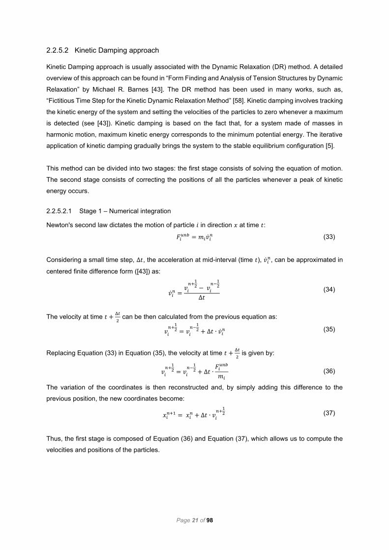
2.2.5.2.1 Stage 1 – Numerical integration
Newton's second law dictates the motion of particle 𝑖 in direction 𝑥 at time 𝑡:
𝐹𝑖𝑢𝑛𝑏 = 𝑚𝑖�̇�𝑖
𝑛 (33)
Considering a small time step, Δ𝑡, the acceleration at mid-interval (time 𝑡), �̇�𝑖𝑛, can be approximated in
centered finite difference form ([43]) as:
�̇�𝑖
𝑛 =𝑣𝑖
𝑛+12 − 𝑣
𝑖
𝑛−12
Δ𝑡
(34)
The velocity at time 𝑡 +Δ𝑡
2 can be then calculated from the previous equation as:
𝑣𝑖
𝑛+12 = 𝑣
𝑖
𝑛−12 + Δ𝑡 ∙ �̇�𝑖
𝑛 (35)
Replacing Equation (33) in Equation (35), the velocity at time 𝑡 +Δ𝑡
2 is given by:
𝑣𝑖
𝑛+12 = 𝑣
𝑖
𝑛−12 + Δ𝑡 ∙
𝐹𝑖𝑢𝑛𝑏
𝑚𝑖
(36)
The variation of the coordinates is then reconstructed and, by simply adding this difference to the
previous position, the new coordinates become:
𝑥𝑖𝑛+1 = 𝑥𝑖
𝑛 + Δ𝑡 ∙ 𝑣𝑖
𝑛+12 (37)
Thus, the first stage is composed of Equation (36) and Equation (37), which allows us to compute the
velocities and positions of the particles.

Page 22 of 98
2.2.5.2.2 Stage 2 – Kinetic Damping approach
Generally, the kinetic energy of undamped oscillations of the structure is traced when a peak in the total
kinetic energy of the system is detected; consequently, all velocities are set to zero. The kinetic energy
of the whole structure is calculated as follows in [58] and can be written as:
𝐾𝑛+1 =1
2∑𝑚𝑖 (𝑣
𝑖
𝑛+12)
2𝑞
𝑖=1
(38)
where 𝐾𝑛+1 is the kinetic energy of the system of particles. 𝑚𝑖 is the mass of particle 𝑖. 𝑣𝑖
𝑛+1
2 is the
velocity of particle 𝑖 and 𝑞 is the number of particles.
In Kinetic Damping approach formulation, a decrease of the kinetic energy indicates that a peak has
been passed [43][58]. At this time, the stored coordinates are 𝑥𝑖𝑛+1, as represented in the figure below.
For simplification, it is assumed that the kinetic energy attains its peak at 𝑡 −Δ𝑡
2 . All particles coordinates
must be then recalculated/restarted at this peak instant.
The coordinate at time 𝑡 −Δ𝑡
2 can be given by subtracting this difference from the previous position.
Thus, the coordinate backward returns to:
𝑥𝑖
𝑛−12 = 𝑥𝑖
𝑛 −Δ𝑡
2 𝑣
𝑖
𝑛−12 (39)
By reorganizing Equation (37), the previous position can be given as follows:
𝑥𝑖𝑛 = 𝑥𝑖
𝑛+1 − Δ𝑡 𝑣𝑖
𝑛+12 (40)
Replacing Equation (40) in Equation (39):
𝑥𝑖
𝑛−12 = (𝑥𝑖
𝑛+1 − Δ𝑡 𝑣𝑖
𝑛+12 ) −
Δ𝑡
2 𝑣
𝑖
𝑛−12 (41)
Finally, replacing Equation (36) in Equation (41), results:
𝑥𝑖
𝑛−12 = 𝑥𝑖
𝑛+1 −3
2 Δ𝑡 𝑣
𝑖
𝑛+12 +
1
2∙𝐹𝑖
𝑢𝑛𝑏
𝑚𝑖
∙ Δ𝑡2 (42)
Figure 2.8 – The trace of a typical kinetic energy peak. Adapted from [93].

Page 23 of 98
When the analysis is restarted, the velocities must be computed at the middle point of the previous
interval. Recalling that the velocity at time t is given by Equation (43), Equation (44) is obtained.
𝑣𝑖𝑛 =
1
2( 𝑣
𝑖
𝑛−12 + 𝑣
𝑖
𝑛+12 ) = 0 (43)
𝑣𝑖
𝑛−12 = −𝑣
𝑖
𝑛+12 (44)
By exploiting Equation (44) and Equation (36), the velocity becomes:
𝑣𝑖
𝑛+12 =
1
2∙𝐹𝑖
𝑢𝑛𝑏
𝑚𝑖
∙ Δ𝑡 (45)
where all unbalanced forces, 𝐹𝑖𝑢𝑛𝑏, must be evaluated at the 𝑥
𝑖
𝑛−1
2 position using Equation (42).
2.3 Numerical implementation of the PSA3D physics engine
This subchapter gives an overview of the numerical implementation of the PSA3D physics engine. It
can be summarized in the Numerical method and the Numerical process.
2.3.1 Numerical method
The Numerical method is the implementation of the Particle System approach (PS), which consists of
solving Newton's second law for a set of particles by numerical integration. The first step is to set the
geometry by defining the list of particles and the list of rods. Then, the equivalent mass for each rod, mα ,
is computed and allocated to each particle in accordance with equations (10) and (11), respectively.
Then, the initial conditions and the stopping criterion are set. Finally, the Numerical process (Annex
B.6.1) can occur until the stopping criterion is met, as summarized in Figure 2.9.
The Numerical process involves the list of particles and the list of rods. It can be summarized in two
fundamental parts, the numerical integration of the equation of motion and the calculation of axial forces
in each rod. The numerical integration of the equation of motion consists of transforming the unbalanced
forces acting on a particle into acceleration, and then, into motion of the particle. As will be explained
later, this process starts by calculating the unbalanced forces for a set of particles, followed by the
accelerations. Then, the new positions and velocities are calculated. Finally, the axial forces of the rods
are calculated.

Page 24 of 98
As follows, two approaches are presented for the implementation of the Numerical process. Approach
1 considers the small displacements formulation and a damping force approach; Approach 2 considers
the large displacements formulation and a kinetic energy damping approach. The following sections will
be considered: Numerical process for Approach 1 and Numerical process for Approach 2.
2.3.2 Numerical process – Approach 1
The Numerical process for Approach 1 consists of looping both the list of particles and the list of rods
(Annex B.6.1). First, the numerical integration is implemented for each particle by applying the
trapezoidal rule. Then, the axial force is calculated for each rod, considering the hypothesis of small
displacements. The figure below shows the Numerical process for Approach 1.
Figure 2.10 – Numerical process – Approach 1 flow chart.
Figure 2.9 – Numerical method flow chart.

Page 25 of 98
2.3.2.1 Numerical integration of the equation of motion
Several numerical integration techniques may be used for solving the equation of motion [59]. The most
common are the Euler’s Method, the Verlet Method, and the Runge-Kutta Method [60]. Sometimes it is
convenient to reformulate the second-order differential equation as a system of two coupled first-order
differential equations [61]. So, by introducing the auxiliary function v(t) into the system and considering
(for the sake of simplicity) the motion of a particle in one dimension, it is now possible to rewrite them in
explicit form as follows:
{
𝑑𝑣
𝑑𝑡= 𝑎(𝑡),
𝑑𝑥
𝑑𝑡= 𝑣(𝑡)
(46)
where 𝑥(𝑡) is the displacement, 𝑣(𝑡) is the velocity and 𝑎(𝑡) is the acceleration at time 𝑡. The differential
equations are to be solved with the initial conditions:
𝑥(𝑡0) = 𝑥0 ; 𝑣(𝑡0) = 𝑣0
Considering the Taylor series expansions for velocity, 𝑣𝑛+1 = 𝑣(𝑡 + 𝛥𝑡) and displacement, 𝑥𝑛+1 =
𝑥(𝑡 + 𝛥𝑡), it follows:
𝑣𝑛+1 = 𝑣𝑛 + 𝑎𝑛𝛥𝑡 + 𝑂((𝛥𝑡)2) (47)
𝑥𝑛+1 = 𝑥𝑛 + 𝑣𝑛𝛥𝑡 +1
2𝑎𝑛(𝛥𝑡)2 + 𝑂((𝛥𝑡)3) (48)
The Euler algorithm is obtained from the above series by truncating the O(∆t) terms (see [61]), resulting
in equations (49) and (50).
𝑣𝑛+1 = 𝑣𝑛 + 𝑎𝑛𝛥𝑡 (49)
𝑥𝑛+1 = 𝑥𝑛 + 𝑣𝑛𝛥𝑡 (50)
The trapezoidal rule is a refinement of Euler's method; it consists of using the mean velocity during the
interval to obtain a new position [60], and its application can be summarized as:
𝑣𝑛+1 = 𝑣𝑛 + 𝑎𝑛𝛥𝑡 (51)
𝑥𝑛+1 = 𝑥𝑛 +1
2(𝑣𝑛 + 𝑣𝑛+1)𝛥𝑡 (52)
All the steps must be repeated for the other directions.
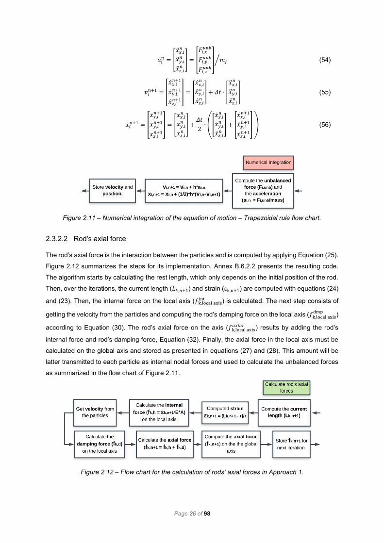
The numerical integration of the equation of motion algorithm in Approach 1 consists of applying the
trapezoidal rule. In this way, the unbalanced forces at the particle are transformed into motion, as shown
in Figure 2.11 and Annex B.6.2.1. In the first step, the unbalanced forces (𝐹𝑖𝑢𝑛𝑏) are calculated, Equation
(53), and then the acceleration (𝑎𝑖𝑛), Equation (54). Later, velocities (𝑣𝑖
𝑛+1) and positions (𝑥𝑖𝑛+1) are
calculated using equations (55) and (56), respectively.
𝐹𝑖𝑢𝑛𝑏 = [
𝐹𝑖,𝑥𝑢𝑛𝑏
𝐹𝑖,𝑦𝑢𝑛𝑏
𝐹𝑖,𝑧𝑢𝑛𝑏]
] = [
𝐹𝑖,𝑥𝑒𝑥𝑡
𝐹𝑖,𝑦𝑒𝑥𝑡
𝐹𝑖,𝑧𝑒𝑥𝑡
] + ∑ ([
𝐹𝑘,𝑥𝑖𝑛𝑡
𝐹𝑘,𝑦𝑖𝑛𝑡
𝐹𝑘,𝑧𝑖𝑛𝑡
])
𝑛
𝑘=1
+ [
𝐹𝑖,𝑥𝑟𝑒𝑎𝑐𝑡𝑖𝑜𝑛
𝐹𝑖,𝑦𝑟𝑒𝑎𝑐𝑡𝑖𝑜𝑛
𝐹𝑖,𝑧𝑟𝑒𝑎𝑐𝑡𝑖𝑜𝑛
] (53)
Page 26 of 98
𝑎𝑖𝑛 = [
�̈�𝑥,𝑖𝑛
�̈�𝑦,𝑖𝑛
�̈�𝑧,𝑖𝑛
] = [
𝐹𝑖,𝑥𝑢𝑛𝑏
𝐹𝑖,𝑦𝑢𝑛𝑏
𝐹𝑖,𝑧𝑢𝑛𝑏
] 𝑚𝑗⁄ (54)
𝑣𝑖
𝑛+1 = [
�̇�𝑥,𝑖𝑛+1
�̇�𝑦,𝑖𝑛+1
�̇�𝑧,𝑖𝑛+1
] = [
�̇�𝑥,𝑖𝑛
�̇�𝑦,𝑖𝑛
�̇�𝑧,𝑖𝑛
] + 𝛥𝑡 ∙ [
�̈�𝑥,𝑖𝑛
�̈�𝑦,𝑖𝑛
�̈�𝑧,𝑖𝑛
] (55)
𝑥𝑖𝑛+1 = [
𝑥𝑥,𝑖𝑛+1
𝑥𝑦,𝑖𝑛+1
𝑥𝑧,𝑖𝑛+1
] = [
𝑥𝑥,𝑖𝑛
𝑥𝑦,𝑖𝑛
𝑥𝑧,𝑖𝑛
] +𝛥𝑡
2∙ ([
�̇�𝑥,𝑖𝑛
�̇�𝑦,𝑖𝑛
�̇�𝑧,𝑖𝑛
] + [
�̇�𝑥,𝑖𝑛+1
�̇�𝑦,𝑖𝑛+1
�̇�𝑧,𝑖𝑛+1
] ) (56)
2.3.2.2 Rod's axial force
The rod’s axial force is the interaction between the particles and is computed by applying Equation (25).
Figure 2.12 summarizes the steps for its implementation. Annex B.6.2.2 presents the resulting code.
The algorithm starts by calculating the rest length, which only depends on the initial position of the rod.
Then, over the iterations, the current length (𝐿𝑘,𝑛+1) and strain (εk,n+1) are computed with equations (24)
and (23). Then, the internal force on the local axis (𝑓 k,local axisint ) is calculated. The next step consists of
getting the velocity from the particles and computing the rod’s damping force on the local axis (𝑓 k,local axisdmp
)
according to Equation (30). The rod’s axial force on the axis (𝑓 k,local axis𝑎𝑥𝑖𝑎𝑙 ) results by adding the rod’s
internal force and rod’s damping force, Equation (32). Finally, the axial force in the local axis must be
calculated on the global axis and stored as presented in equations (27) and (28). This amount will be
latter transmitted to each particle as internal nodal forces and used to calculate the unbalanced forces
as summarized in the flow chart of Figure 2.11.
Figure 2.11 – Numerical integration of the equation of motion – Trapezoidal rule flow chart.
Figure 2.12 – Flow chart for the calculation of rods’ axial forces in Approach 1.

Page 27 of 98
2.3.3 Numerical process – Approach 2
Similarly to Approach 1, the Numerical process for Approach 2 consists of looping in sequence the list
of particles and the list of rods (Annex B.6.1). First, the numerical integration is carried out for each
particle by applying the centered finite difference. Then, the Kinetic Damping step is applied. Finally, the
axial force is calculated for each of the rods, considering the formulation for large displacements. The
figure below shows the Numerical process for Approach 2.
2.3.3.1 Stage 1 – Numerical integration
As referred before, the relationship between the velocity, the position, and the unbalanced forces can
be obtained by performing a double numerical integration of the acceleration. For Approach 2, this step
can be performed using the central finite difference form [43].
Figure 2.14 and Annex B.6.3.1 summarize the implementation of the numerical integration in Approach
2. It starts by computing the unbalanced force (𝐹𝑖𝑢𝑛𝑏) and the acceleration (𝑎𝑖
𝑡 =𝐹𝑖
𝑢𝑛𝑏
𝑚𝑖). The next step is
to check if it is a peak. In case it is a peak, the velocity at the mid-point (𝑣𝑖
𝑛+1
2) is calculated with Equation
(45). Otherwise, the velocity is calculated with Equation (36). Finally, the position (𝑥𝑖𝑛+1) is computed
with Equation (37). As described in [43], the first iteration may be set as a peak and the velocity can be
calculated with Equation (45).
Figure 2.13 – Numerical process – Approach 2.
Figure 2.14 – Stage 1 of the Kinetic Damping approach - Numerical integration flow chart.

Page 28 of 98
2.3.3.2 Stage 2 – Kinetic Damping approach
The stage 2 of the Kinetic Damping approach consists of re-initializing the velocities at kinetic energy
peaks. The figure below summarizes its implementation, and Annex B.6.3.1 presents the resulting code.
The algorithm starts by computing the current kinetic energy (𝐾𝑛+1) according to Equation (38). Then,
the current kinetic energy is compared with the previous ones. If condition 𝐾𝑛−1 ≤ 𝐾𝑛 𝑎𝑛𝑑 𝐾𝑛 ≤ 𝐾𝑛+1 is
not met, it means that a peak occurs between t1 = 𝑡 − Δ𝑡 and t2 = 𝑡, and the position of each particle
must be reevaluated at the position 𝑥𝑖
𝑡−Δ𝑡
2 , according to Equation (42). Finally, the kinetic energy is reset
to zero.
2.3.3.3 Rod's axial force
Considering the formulation for large displacements, the rod’s axial force can be given by Equation (25)
and is conveniently recalled here as:
𝑓 k,local axisint = (σk,nAn + EnAnεk,n+1)e1′2′
εk,n+1 =ΔL
Lk,n
=Lk,n+1 − Lk,n
Lk,n
Figure 2.15 – Stage 2 of the Kinetic Damping approach – flow chart.

Page 29 of 98
The axial force in each rod can be summarized as presented in Figure 2.16. Annex B.6.3.2 presents the
resulting code. The algorithm starts by calculating the current length of the rod 𝑘, 𝐿𝑘,𝑛+1, and the
transformation matrix with the approach presented in Equation (22). Then, the strain (εk,n+1) is
computed. Finally, the axial force in the local axis (𝑓 k,local axisint ) can be calculated. As presented before,
the axial force must be calculated on the global axis and stored as presented in equations (27) and (28).
This amount will be latter transmitted to each particle as internal nodal forces and used to calculate the
unbalanced forces, as summarized in the flow chart of Figure 2.14. For further iterations, the current
stress, σk,n+1 = 𝑓𝑘,𝑛+1
𝐴𝑛, is calculated and stored along with 𝐿𝑘,𝑛+1.
2.4 Stopping criterion
An iterative numerical method is used to solve Newton's second law. Thus, this approach calculates
successive approximations for the solution of the differential equation (9), which is recalled here for
convenience.
𝑚𝑖 [
�̈�𝑖,𝑥
�̈�𝑖,𝑦
�̈�𝑖,𝑧
] = [
𝐹𝑖,𝑥𝑒𝑥𝑡
𝐹𝑖,𝑦𝑒𝑥𝑡
𝐹𝑖,𝑧𝑒𝑥𝑡
] + [
𝐹𝑖,𝑥𝑖𝑛𝑡
𝐹𝑖,𝑦𝑖𝑛𝑡
𝐹𝑖,𝑧𝑖𝑛𝑡
] + [
𝐹𝑖,𝑥𝑟𝑒𝑎𝑐𝑡𝑖𝑜𝑛
𝐹𝑖,𝑦𝑟𝑒𝑎𝑐𝑡𝑖𝑜𝑛
𝐹𝑖,𝑧𝑟𝑒𝑎𝑐𝑡𝑖𝑜𝑛
] = [
𝐹𝑖,𝑥𝑢𝑛𝑏
𝐹𝑖,𝑦𝑢𝑛𝑏
𝐹𝑖,𝑧𝑢𝑛𝑏
]
Such a method involves a sequence of generated steps, an error tolerance, and at each step, an amount
that may be related to the simulation error is estimated. Therefore, numerical methods for ordinary
differential equations have a stopping criterion that can be simply described as in Equation (57) [75].
|휀 − 휀𝑛| < 𝑇𝑜𝑙𝑒𝑟𝑎𝑛𝑐𝑒 (57)
In the case of the 3D force system, the cartesian approach first requires the definition of the x, y, and z
directions. Then, the equations of motion for each direction must be verified. Thus, the presented
stopping criterion uses the unbalanced force of each particle, 𝐹𝑢𝑛𝑏, as a numerical method convergence
indicator. This amount corresponds to the unbalanced forces at each particle that generates the nodal
acceleration, which keeps the numerical method working. However, it is a difficult task to choose a single
meaningful error tolerance, since it mainly depends on the geometry of the structural systems – besides,
the combination of different load scenarios may lead to very different results.
Figure 2.16 – Flow chart for the calculation of rods’ axial forces in Approach 2.
.

Page 30 of 98
The stopping criterion proposed here is:
|𝐹𝑖𝑢𝑛𝑏| ≤ 𝑇𝑜𝑙𝑒𝑟𝑎𝑛𝑐𝑒 (58)
𝐹𝑖𝑢𝑛𝑏 = 𝐹𝑖
𝑒𝑥𝑡 + 𝐹𝑖𝑖𝑛𝑡 + 𝐹𝑖
𝑟𝑒𝑎𝑐𝑡𝑖𝑜𝑛 (59)
where 𝐹𝑖𝑢𝑛𝑏 is the unbalanced force in axis 𝑖, 𝐹𝑖
𝑒𝑥𝑡 is the applied external force, 𝐹𝑖𝑖𝑛𝑡 is the internal nodal
force and 𝐹𝑖𝑟𝑒𝑎𝑐𝑡𝑖𝑜𝑛 is the contribution of the support reaction. The formulation of these quantities was
expressed before in this chapter.

Page 31 of 98
3 The 3DParticleSystem Software
Many commercial and didactic software allow static structural analysis through the direct stiffness
method or finite element analysis (FEA); notable examples are FTOOL [46], ADINA [47], and SAP 2000
[48]. On the other hand, it is not so common to find structural analysis software implemented with
numerical approaches usually found in computer games. The herein developed software, called
3DParticleSystem, adds some diversity to the didactic software commonly used in civil engineering
courses. It is noteworthy that the developed software allows physically nonlinear analysis by considering
nonlinear material models such as the elastic-perfectly plastic model and the bilinear hardening model.
In this chapter, the structure of the developed software and some of its features will be presented.
The PSA3D physics engine (PE) (see Chapter 2) is combined with a graphics rendering middleware –
our own graphics rendering engine, which uses the Panda3D rendering capabilities [44], and is
responsible for rendering the structural engineering phenomena, such as deformation, stress-strain
curves, and even collapse. The result of this combination is the 3DParticleSystem software developed
in this work. This software gives to the user a unique game-like interaction where structural models
respond to input in real-time.
3.1 The 3DParticleSystem GUI
The 3DParticleSystem graphical user interface (GUI) contains some features that are essential for
executing the numerical approach presented in Chapter 2. This section summarizes some important
features needed to use the developed software correctly. The first set of features is related to physical
units. Then the camera control is presented, followed by a general presentation of the 3DParticleSystem
GUI. Finally, some features of the 3DParticleSystem Canvas are presented.
3.1.1 Units
Typically, the software that handles physical phenomena requires the use of length, force, mass, and
time. Therefore, for the 3DParticleSystem software, the units of the physical quantities must be imported
and are exported as follows in Table 3.1.
Table 3.1 – The units needed for the 3DParticleSystem software input.
Units
Length meter (m)
Forces kilonewton (kN)
time second (s)
Mass kilogram (kg)
Area m2
Mass per unit volume kg/m3
Young's modulus GPa
Pressure, stress, etc. MPa

Page 32 of 98
3.1.2 Camera control
The 3DParticleSystem software’s mouse control is like the standard Panda3D’s camera control system.
Table 3.2 shows some keys to handling the navigation in the developed software.
Table 3.2 – Default Panda3D’s camera control system.
Key Action Alternative (Windows 10)
Left Button Pan left and right. -
Right Button Move forward and backward. Control+Left Button
Middle Button Rotate around the origin of the application.
Shift+Left Button
Right and Middle Buttons
Roll the point of view around the view axis.
Control+Shift+Left Button
3.1.3 The 3DParticleSystem GUI overview
The 3DParticleSystem software has two main windows, the menu window, and the canvas window. The
first deals with the menu commands, allowing the user to access the different options of software and
setting the different system variables. The latter deals with the graphical rendering of the structural
system.
3.1.3.1 The 3DParticleSystem menu
Figure 3.1 presents the main menu of the 3DParticleSystem. The menu is divided into several boxes,
namely, the simulation menu, the change structure menu, the choose particle menu, the stopping criteria
menu, the rendering menu, the output menu, and the physical parameters menu. The file option shows
some basic features for handling the input file, such as creating a new model, open file, save file, save
as, export, exit, open from CSV, import from DXF. The features on the left side allow the user to reset
and update the structural system. It also allows the user to remove rods and change support constraints.
On the right side, the user has several features to deal with the parameters of the physics engine and
with the parameters of the graphical rendering engine. The right-side features are combined as:
a) Stopping criterion, which allows setting the stopping criterion.
b) Rendering, which allows setting some auxiliary parameters, such as the axial diagram scale,
the deformed shape scale, the rendering frequency, and the text scale size.
c) Output, which allows the user to show/hide the original geometry of the structure. It also offers
an option to show the stress-strain curve of any rod.
d) Physical Parameter, which allows setting the damping coefficient and the time-step.

Page 33 of 98
3.1.3.2 The 3DParticleSystem Canvas
The 3DParticleSystem Canvas consists of a window with the Grid button and the Simulation button, in
which the structural system is rendered along with its output results. The Grid button allows the user to
show/hide the grid and the axes, being useful for designing the structures and analyzing the output
results. Each axis is represented with a different color; the red, green, and blue lines correspond to the
axes x, y, and z, respectively. The Simulation button controls the state of the simulation. When this
button is clicked, the simulation occurs until a given stopping criterion is met or the state of the simulation
is changed to pause. Figure 3.2 shows a space tower with a square base, and a horizontal load applied
to the top. The following figures sequence graphically shows the evolution of the space truss system
while using the 3DParticleSystem software. These figures show the support reactions as green arrows
and the loading force as a blue arrow. The red bars are subject to tensile stresses, and the blue bars
are subject to compressive stresses.
Figure 3.1 – The 3DParticleSystem software menu.
Figure 3.2 – (a) space tower with a square base. (b) deformed shape with the original structure in the
back. (c) deformed shape.

Page 34 of 98
3.1.3.3 Setting the 3DParticleSystem Software
The 3DParticleSystem's GUI aims to avoid the feeling of learning software from scratch by creating a
software-inspired GUI commonly used by civil engineering students. Thus, some software such as
FTOOL [46], ADINA [47], SAP2000 [48], and AutoCAD [62] played a key role in this creative process.
Before launching the 3DParticleSystem, the user must edit the main input file for the input parameters.
It consists of setting some essential parameters, as presented in Annex A.2. The user must then write
an input file that contains the desired geometry, Annex A.2 (this can be either TXT or CSV). During the
simulation, the user can edit the structure geometry, forces, and constraints using the GUI, and proceed
with the simulation, considering those changes.
When using structural analysis software, the first step is to define the geometry of the structure to be
analyzed. In the developed, it can also be done by editing tables in which points and lines are specified.
As with ADINA (Automatic Dynamic Incremental Nonlinear Analysis [63]), the definition of points and
lines in the 3DParticleSystem software is first given by defining the points and then the lines. Thus, for
each line, the user must choose the corresponding edges from the points already defined.
Figure 3.3 shows the plane truss structure that will be analyzed by the 3DParticleSystem software. All
rod elements are considered to have the same cross-sectional area of 20 cm2 , elastic modulus 𝐸 =
200 𝐺𝑃𝑎 and mass per unit volume 𝜌 = 7900 𝑘𝑔 𝑚3⁄ . Then, the mass per unit length of the rod element
is 𝜆 = 𝜌𝐴 = 15.8 𝑘𝑔 𝑚⁄ . The system is loaded with an applied force of 100 kN along the z-axis at nodes
B, C, E, F and G.
Figure 3.3 – Plane truss. Adapted from FTOOL.

Page 35 of 98
Figure 3.4 and Annex A.2 show the definition of the geometry of the plane truss structure by editing two
tables, one for particles and one for rods. Figure 3.4 in the left shows the particles named from A to G,
along with its coordinate. Figure 3.4 in the right shows the rod named from 1 to 11. Each rod is composed
by two particles, for exemple, rod10 results from the connection of ParticleC and ParticleE.
Then, it is just a matter of editing the input tables to define support constraints and external forces, as
shown in Figure 3.5. This step can be made at any time during the simulation.
Figure 3.5 – An example of defining support constraints and external forces in the 3DParticleSystem
software.
Figure 3.4 – Definition of particles and rods in the 3DParticleSystem software.

Page 36 of 98
The next step is to define the cross-sectional area, mass per unit volume, and the modulus of elasticity
or the stress-strain curve, Figure 3.6.
After the simulation, the numerical results can be displayed as output tables and graphs, as shown
below. Figure 3.7 shows the computed results for a set of particles. Figure 3.8 and Figure 3.9 show the
stress-strain curve for some bars (rod6 and rod10) with their results (axial force, strain, and stress).
Figure 3.7 – The results of the particles in the 3DParticleSystem software.
Figure 3.6 – An example of defining the cross-sectional area and the material’s mechanical properties
in the 3DParticleSystem software.

Page 37 of 98
The 3DParticleSystem software has some computer-aided design (CAD) capabilities. Still, it may be
more advantageous to use an advanced CAD/drafting software such as AutoCAD to design the structure
geometry. In this way, the resulting files in the DXF format (AutoCAD 2018 Drawing Exchange Format)
can be imported from AutoCAD applications to the 3DParticleSystem software, as shown in Figure 3.10.
Figure 3.9 – The results of stress and strain in the 3DParticleSystem software.
Figure 3.10 – Importing from AutoCAD 2018 to the 3DParticleSystem software.
Figure 3.8 – The results of the rods in the 3DParticleSystem software.
Exporting as .dxf Importing as .dxf

Page 38 of 98
3.2 Software structure
This subsection explains some topics related to the structure of the developed software. This subsection
starts by presenting the tools chosen for this task, Python and Anaconda. Then, the structure of the
3DParticleSystem is presented. Finally, some aspects related to the implementation of the physics
engine are presented.
3.2.1 Python and Anaconda
Python is often the first programming language engineering science students are exposed to. In
addition, it is one of the fastest-growing platforms for machine learning. This versatility is one of the
advantages of this programming language. Besides, Python has excellent online learning resources and
is becoming an increasingly popular programming language in many areas due to its large standard
library, expressive syntax, and focus on code readability [13]. Python is a high-level, interpreted, cross-
-platform, and dynamically typed programming language that supports different programming
paradigms, such as the functional paradigm and the object-oriented paradigm.
Despite all the advantages above described, a user with poor programming skills may have some
difficulties installing packages and programming libraries; these tasks can be daunting and even slow
the learning progress. However, these difficulties can be easily overcome by using the Spyder IDE and
Anaconda [64] or other similar environments. Anaconda is a highly recommended alternative to the
Python distribution for scientific computing, ideal for a novice user who does not know which packages
will be needed.
3.2.2 The 3DParticleSystem structure
The 3DParticleSystem software is entirely written in Python and allows the user to draw structures,
analyze them, and then export the results. The CAD software has been successfully created from
scratch. Thus, the developed software is organized into two distinct modules: one implementing the GUI
and the other implementing for the PSA3D physics engine, described in Chapter 2. The
3DParticleSystem GUI was created using two frameworks: PyQt framework and Panda3D game engine.
The first is responsible for managing the main features available to the user, such as buttons and menus.
The latter is responsible for handling the graphics rendering engine, rendering the geometry of the
structure, and presenting numerical results.
The 3DParticleSystem software starts with a simple main file, which is a Python Main function and is
presented in Annex B.1. This main method calls the Qt application and the 3DParticleSystem Graphical
User Interface (GUI) (class The3DParticleSystemGUI), Annex B.2. The 3DParticleSystem GUI launches
the 3DParticleSystem main menu, presented in Figure 3.1 (The3DPsDialog class, Annex B.3), starting
the event-loop [65] until the PyQt Application is closed. Then, the 3DParticleSystem Graphical User
Interface instantiates the game engine (class GameEngine3DParticleSystem). The game engine uses
its Elements‘ instance (PSA3DElements) to read the structural system file with the structural geometry

Page 39 of 98
and saves its content as a list of elements (particles and rods), Annex B.4.1. After reading the input file,
the class Element (PSA3DElements) calls the private method named initStructureSystem (Annex B.5.1),
which loops through the list of elements (particles and rods), and, for each element, two objects are
created, one that handles physical properties (Annex B.6.2 and B.6.3) and the other graphical properties
(Annex B.7.3 and B.7.4). After the graphical part element is created, it is also added to the canvas
(Annex B.5.2 and B.5.3).
Normally, the game engine has its own event-loop. The game loop of Panda3D is based on the concept
of tasks [66]. The tasks are like threads and state the game mode on each loop, for example, either the
game is running or not. Thus, the developed software uses a task to control whether the PSA3D physics
engine (PE) is running or not, and also to stop the numerical method once the stopping criterion is met
(Annex B.4.2 and B.6.1).
The 3DParticleSystem software interacts with the user from a simple window developed with the Qt
framework, namely, the 3DParticleSystem GUI main menu (Annex B.2). Then, by controlling the Qt, the
user has control of the game engine (Annex B.4), which handles the PSA3D PE (Annex B.6) and the
GRE (Annex B.7). Thus, the user can change the state of the simulation at any time, as well as using
all the features available in the developed software. Figure 3.11 summarizes the overall responsibilities
of each module. Besides, it presents the communication between the different modules.
The double arrow represents that the user can interact with the 3DParticleSystem GUI (Annex B.2). and
with the 3DParticleSystem GE (Annex B.4), throughout the canvas. Besides, it allows the user to control
features from the canvas, such as the deformed structural scale, axial diagram scale, grid, and camera.
Moreover, the PSA3D PE (Annex B.6) gets the properties from the elements and runs the numerical
simulation. Then, over the simulations, it updates the numerical data of each element. On the other
hand, the GRE handles all the logic behind rendering the space trusses in the canvas.
Figure 3.11 – Communication among the user and different modules (GUI, GE, PE, and GRE).

Page 40 of 98
3.2.3 Physics engine programming challenges
During the development of the PSA3D physics engine, there were some programming challenges, two
of which stand out: computational performance and maintaining a friendlier programming framework. In
this way, auxiliary functions have been written in Python to do basic algebraic operations, corresponding
to a thin layer between algebraic operations and Python NumPy [67], allowing for algebraic operations
such as sum, addition, and product of vectors and matrices. Among these functions, two stand out,
Matrix Operations and Transformation Functions.
Matrix Operations are a set of auxiliary functions that aim to create and manipulate Python arrays (Annex
B.8.1). These functions allow the PSA3D physics engine to perform matrix operations such as sum,
addition, and product. Transform Functions are a set of auxiliary functions that allow the PSA3D physical
engine to handle transformation matrices, allowing operations such as the calculation of unit vectors,
cross products, and transformation matrices (Annex B.8.2).
3.3 Qt framework and PyQt
The 3DParticleSystem GUI goal is to give the best usability in the fewest clicks possible. It also seeks
to reduce the learning curve of the developed software. Thus, the developed software uses the PyQt
framework for this purpose. Qt is a cross-platform framework to develop GUI in C++ that was produced
by the Norwegian company Trolltech and, since 2008, is owned by Nokia. The latest version of Qt is
5.12 LTS, released December 6, 2018, and supported for three years [68]. PyQt brings together the
cross-platform language Python and the Qt C++ cross-platform application framework [45].
Qt is based on a well-known Signal & Slot paradigm [69]. In this, the buttons have a callback that
corresponds to the function of the button. The simplest example is the "Exit" button, which calls the exit
method and allows the user to exit the program. Therefore, this paradigm links GUI features such as
buttons, tabs, and combo boxes to its respective callback. Thus, Python’s data structure, such as
dictionary and list, are widely used in the developed GUI, making easy some tasks such as the signal
and callback task, allowing to connect each widget to its respective callback directly.
3.4 Panda3D
This subchapter gives a brief description of Panda3D, introducing some of its essential features.
Besides, it gives an overview of the implementation of the drawing the elements: particles and rods.
3.4.1 Brief Panda3D description and basic features
The engine developed by Disney Interactive to create one of its attractions later became the Panda3D
game engine. Before that, some popular commercial games such as Toontown (2003), Pirates of the
Caribbean Online (2007), and A Vampyre Story (2008) were developed using this tool [70]. Panda3D is
a 3D game engine, a library of subroutines for 3D rendering and game development. It is open-source

Page 41 of 98
and free for any purpose, even commercial [70], allowing the creation of games through programs
written in Python or C ++ using Panda3D libraries. Annex A shows how to install Panda3D.
Although Panda3D has many features, the use of this framework in the 3DParticleSystem software is
minimal as it is not intended to limit the development of this software to the game engine used in this
release. The developed CAD software is based on rendering a set of organized lines, which makes it
possible to render arrows, circles, grids, nodes, and bars — then building all the needed modules to
represent structures with complex geometries.
One of the most important concepts of the graphics rendering engine is Canvas, shown in Figure 3.12.
This can be described as the area or screen in which all UI elements should be contained [71]. Thus, it
usually has several methods for drawing lines, boxes, circles, text, and adding images. In Panda3D,
ShowBase can be considered a Canvas.
3.4.2 ShowBase class
The ShowBase class or DirectStart ShowBase is a Panda3D application framework responsible for
opening the graphical display window, shown in Figure 3.12. In addition, it is responsible for setting up
the 3D scene graph, input devices, and other elements needed to render the scene graph to the window,
such as camera, keyboard, and mouse control [72]. Moreover, this class creates buttons, sliders, and
text.
3.4.3 LineNodePath class
LineNodePath class is a fundamental class from Panda3D packages, inheriting from the NodePath class
[73] and allowing the user to render lines by giving as input arguments, thickness, and color (Annex
B.7.1). It is then possible to set the starting and ending points for the line by using public methods of
LineNodePath class. Figure 3.13 shows the inheritance diagram for the LineNodePath class.
Figure 3.12 – GUI window of Panda3D ShowBase.

Page 42 of 98
It is now possible to extend the LineNodePath class to create smarter objects, empowering the
developed CAD with functionalities essential to its operation.
3.4.4 ElementaryLine, ElementaryArc and Arrow classes
By arranging lines using pure mathematical logic, it is then possible to render arrows, arcs, circles,
triangles, and rectangles. Then, by combining all these simple geometric elements, it is possible to
render structural systems with different complexities. Thus, the development of a graphics rendering
engine begins by creating the line class, called the ElementaryLine class.
3.4.4.1 ElementaryLine class
The ElementaryLine class is an extension of the LineNodePath class (Annex B.7.1) and receives not
only the starting and ending points for the line but also the color and thickness (Annex B.7.2). This
extension includes methods that allow changing color and thickness, as well as updating the
coordinates, making it easier to render the most crucial element in this graphical interface. Figure 3.14
shows a representation of the lines in a simple Panda3D application and the respective code is
presented in Annex B.7.1.
3.4.4.2 ElementaryArc and Arrow classes
The ElementaryArc class is an extension of the LineNodePath class and can render arcs and circles by
specifying a center and a radius. Moreover, the Arrow class is another extension of the LineNodePath
class and allows the developed CAD to graphically represent arrows by specifying the starting and
ending points, color, and thickness. Figure 3.15 shows the representation of lines, arrows, and circles
in the 3DParticleSystem software.
Figure 3.14 – Rendering an ElementaryLine object in a simple Panda3D application.
Figure 3.13 – Inheritance diagram for LineNodePath class. Adapted from [88].

Page 43 of 98
3.4.5 GameEngine3DParticleSystem class
The GameEngine3DParticleSystem class brings together all the elements that make up the graphics
rendering engine (Annex B.4). The function of the GameEngine3DParticleSystem can be summarized
in:
a) Start the DirectStart ShowBase,
b) Start and handle the Graphics Rendering Engine and the screen,
c) Start the grid and define Panda 3D events, such as the escape button, the simulation/stop
button, and the grid button,
d) From the resource files, obtain the input parameters, such as the stop/tolerance criteria for the
simulation, the Physics Engine parameters and the type of approach, Approach 1 or 2,
e) Start and handle the PSA3D physics engine.
3.5 Elements
The Particle System approach discretizes the space truss structure into simple elements such as
particles and rods, as described in Figure 3.16. Thus, for the computational implementation of these
elements, the Elements class was created (Annex B.5). When particles and rods are created, this class
divides each element into its graphical (Annex B.7.3 and B.7.4) and physical parts (Annex B.6.2.2 and
B.6.2.1), with the geometry being the linking attribute between these parts.
The first step in rendering a structure is to create particles that define it. Thus, the Element class must
receive the coordinates of each particle, being the result presented in Figure 3.17, on the left. Then it is
possible to create a bar/rod element. Figure 3.17 shows, on the right, the plane truss structure
representation in the 3DParticleSystem software.
Figure 3.15 – Representation of lines, arrows, and circles in the 3DParticleSystem software.

Page 44 of 98
3.5.1 Particles
The particle element carries properties such as coordinates, nodal constraints, and external forces.
Then, as a programming approach, each particle is implemented as having physical and graphical
components. Regarding the representation of particle elements, it can be a constraint or a loaded node.
This is organized into two distinct classes, NodalConstraint and ExternalForce (Annex B.7.3).
3.5.1.1 NodalConstraints class
Constraints are limits to the motion of particles. The most common 3D nodal constraints are roller
constraints, ball-and-socket joints, and ball joints. Therefore, the class that handles the graphical
representation of nodal constraints is called Nodal Constraint and imports classes such as
LineNodePath, ElementaryArc, and ArrowAlongAxis. Figure 3.18 shows the graphical representation of
different types of nodal constraints in the 3DParticleSystem software.
Figure 3.18 – Different types of nodal constraints in the 3DParticleSystem software. From left to right,
ball joint in X0Y and Y0Z, roller along y and x, ball-and-socket joint.
Figure 3.16 – (a) plane truss structure; (b) discretization of the structure in particles and rods.
Figure 3.17 – Graphical representation of the particles, on the left, plane truss structure, on the right.

Page 45 of 98
3.5.1.2 ExternalForce class
Force is an interaction between bodies and is typically represented by vectors. In addition, vectors are
a geometric object that has magnitude, direction, and an application point. The class that handles
external forces is called the ExternalForce class and imports the Arrow class. Figure 3.19 shows on the
left the external forces represented by blue arrows; On the right, the supports are also represented and
their respective reactions, by green arrows.
3.5.2 Rod
Each rod element can be discretized into two particles that contain all their intrinsic properties, namely,
original position, deformed position, nodal constraints, and external forces. These coordinates are then
used to calculate the rod’s length and the local-to-global transformation matrix. Furthermore, each rod
must also receive physical parameters, such as the cross-sectional area, the stress-strain curve, and
mass per unit volume. It is then possible to characterize the mass of the rod that will be used to compute
the mass of each particle, according to equations (10) and (11).
Rods are organized into three classes, namely, ElementaryRod, AxialDiagram, and DeformedRod
(Annex B.7.4). Even though having common attributes, they have very distinct meanings.
3.5.2.1 ElementaryRod class
The ElementaryRod class extends the ElementaryLine class, giving 3DParticleSystem software the
ability to render rods. This class takes as its argument two coordinates, along with its rendering
properties, color, and thickness. The graphical representation of any rod begins by specifying its original
geometry and can be updated at any time using its public methods.
3.5.2.2 DeformedRod class
DeformedRod class allows 3DParticleSystem software to render the deformed shape of any structure.
To do this, this class inherits basic rendering properties from ElementaryLine and ElementaryRod, to
control color and scale.
Figure 3.20 shows, on the left, the structure with its deformed shape; on the right, it shows the same
structure without the original form. The graphical representation of a deformed rod is usually based on
its axial force since the structure system changes color according to the magnitude of this parameter.
Besides, the DeformedRod class allows the user to amplify the deformed shape by controlling a single
Figure 3.19 – Representation of external forces (left). Representation of a complete plane truss with
reaction support results (right).

Page 46 of 98
amplification scale parameter. Then, as a property of the ElementaryRod class, it is possible to hide the
original form, which is very useful when graphically analyzing complex structural systems.
3.5.2.3 AxialDiagram
The next step is to render the axial force diagram. Such a diagram has a standard form of representation,
so some algebraic manipulation is required to do it properly. It is also useful to introduce a text along
with the diagram, which allows the user to track the values of axial forces throughout the evolution of
the system. Thus, the AxialDiagram class handles the axial force diagram representation, by importing
DeformedRod and RendText classes, the latter being responsible for rendering text in the canvas.
Figure 3.21 shows an example of an axial force diagram in the 3DParticleSystem software.
3.6 Simulation mode
The game loop is the overall flow control for the entire game program, where the game continues
performing a series of actions until the user quits [74]. The 3DParticleSystem software game loop
consists of the physical engine constantly doing the math according to the loop shown in Figure 2.9,
regardless of the graphics rendering engine, until a defined stopping criterion is met. On the other hand,
the graphics rendering engine is updated as often as the user deems necessary by controlling the GUI
parameter named rendering frequency, which quantifies how often the physics engine updates the
graphics rendering engine.
The communication between the physics engine (Annex B.6) and the graphics rendering engine (Annex
B.7) plays an essential role in the interactivity of the 3DParticleSystem software throughout the class
Elements. The PE refreshes the Elements’ GR. Later, the Element class updates the GRE. In this way,
the GRE updating is controlled by the physics engine simulation status. This updating is very
Figure 3.21 – Axial force diagram of a plane truss structure in the 3DParticleSystem.
software.
Figure 3.20 – The deformed and the original shape of a plane truss structure in the 3DParticleSystem
software on the left. The deformed shape without the original shape on the right.

Page 47 of 98
straightforward and involves numeric and graphic parts. The communication between these parts has
some complexity in the methods that are called. The rendering method starts by accessing the numeric
attributes of each element and then updates the graphical environment based on these values (Annex
B.5.4). It consists of two main loops, a loop in the rod list and another in the particle list. The first loop
consists of updating the axial force of the rods and refreshing the current position of the two particles
that make up the rod. The second loop consists of updating new support reaction arrows, according to
the support reaction values.

Page 48 of 98
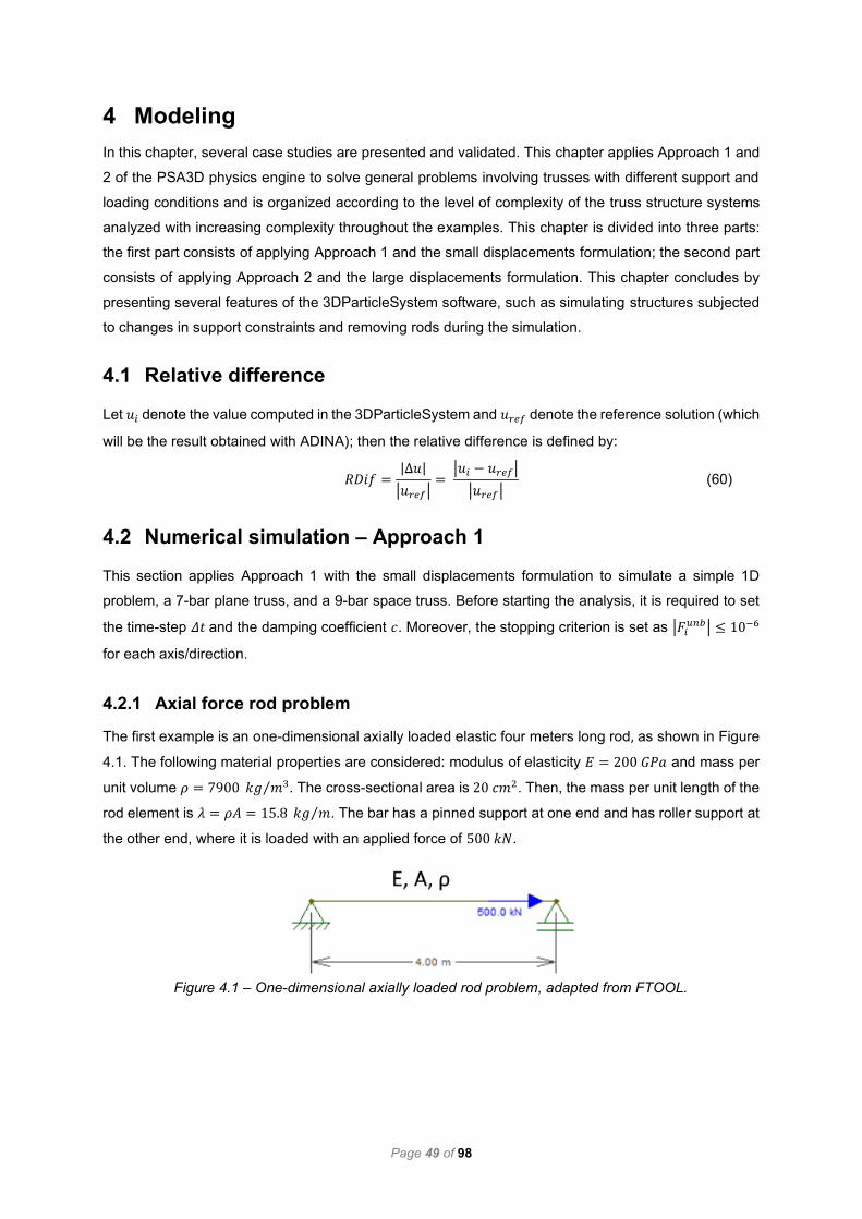
Page 49 of 98
4 Modeling
In this chapter, several case studies are presented and validated. This chapter applies Approach 1 and
2 of the PSA3D physics engine to solve general problems involving trusses with different support and
loading conditions and is organized according to the level of complexity of the truss structure systems
analyzed with increasing complexity throughout the examples. This chapter is divided into three parts:
the first part consists of applying Approach 1 and the small displacements formulation; the second part
consists of applying Approach 2 and the large displacements formulation. This chapter concludes by
presenting several features of the 3DParticleSystem software, such as simulating structures subjected
to changes in support constraints and removing rods during the simulation.
4.1 Relative difference
Let 𝑢𝑖 denote the value computed in the 3DParticleSystem and 𝑢𝑟𝑒𝑓 denote the reference solution (which
will be the result obtained with ADINA); then the relative difference is defined by:
𝑅𝐷𝑖𝑓 =|Δ𝑢|
|𝑢𝑟𝑒𝑓|=
|𝑢𝑖 − 𝑢𝑟𝑒𝑓|
|𝑢𝑟𝑒𝑓| (60)
4.2 Numerical simulation – Approach 1
This section applies Approach 1 with the small displacements formulation to simulate a simple 1D
problem, a 7-bar plane truss, and a 9-bar space truss. Before starting the analysis, it is required to set
the time-step 𝛥𝑡 and the damping coefficient 𝑐. Moreover, the stopping criterion is set as |𝐹𝑖𝑢𝑛𝑏| ≤ 10−6
for each axis/direction.
4.2.1 Axial force rod problem
The first example is an one-dimensional axially loaded elastic four meters long rod, as shown in Figure
4.1. The following material properties are considered: modulus of elasticity 𝐸 = 200 𝐺𝑃𝑎 and mass per
unit volume 𝜌 = 7900 𝑘𝑔 𝑚3⁄ . The cross-sectional area is 20 𝑐𝑚2. Then, the mass per unit length of the
rod element is 𝜆 = 𝜌𝐴 = 15.8 𝑘𝑔 𝑚⁄ . The bar has a pinned support at one end and has roller support at
the other end, where it is loaded with an applied force of 500 𝑘𝑁.
Figure 4.1 – One-dimensional axially loaded rod problem, adapted from FTOOL.

Page 50 of 98
The first step in applying the PS approach is to discretize the system into two (or more) particles and
one (or more) rod, as described in Chapter 2. Then, the particle masses should be calculated according
to Equation (10). In this case, it can be discretized into two particles and a rod. Some geometrical
parameters, such as position and mass, are presented in the tables below.
Table 4.1 – Particles A and B, and their properties.
Particle x (m) y (m) m (kg)
A 0 0 31.60
B 4 0 31.60
Table 4.2 – Rod 1 and its properties.
Rod PA PB L (m) m (kg)
1 A B 4 63.20
4.2.1.1 Particle B (roller support)
As expected, Particle B changes its position to solve Newton's equation of motion. As shown in Figure
4.2, the deformed position of the particle changes over iterations until it meets the stopping criterion.
Figure 4.2 shows that it takes around 50 iterations to compute a good approximation of the relative
displacement, with the relative difference being around 0.05% (4.98 mm).
The unbalanced force creates acceleration and velocity in Particle B, which constantly changes its
position. Figure 4.3. shows that, at the first iteration, the unbalanced force is the total external force
applied. Then, over iterations, this unbalanced force is transformed into the motion of the particle. This
motion leads to internal/axial forces that are then placed back at the particle, leading to a new and
smaller unbalanced force. After around 25 iterations, the motion is almost null, and the unbalanced force
is minimal.
Figure 4.2 – Displacement at Particle B (Δt = 2x10⁻⁴ s and c = 200 kN ∙s/m).

Page 51 of 98
Figure 4.4 shows, on the left, the deformed structure; on the right, the stress-strain curve of Rod 1, with
the blue dot being the stress-strain pair after 120 iterations.
4.2.1.2 Particle A (pinned support)
The system has a pinned support at Particle A. Thus, all the axial forces generated by the motion of the
Particle B are transmitted to Particle A throughout the rod. As Particle A is constrained, a support
reaction arises that balances out the axial force. Figure 4.5 shows two symmetric curves representing,
respectively, the axial force and the reaction at the support. After 25 iterations, there is already a good
approximation for the support reaction, which is 500 kN.
Figure 4.3 – Nodal Forces in Particle B (Δt = 2x10⁻⁴ s and c = 200 kN ∙s/m).
Figure 4.4 – The deformed shape, amplified 100x (left). Stress-strain curve after 120 iterations (right).

Page 52 of 98
4.2.1.3 Rod 1
Figure 4.6 shows the evolution of the axial force over the iterations. For a bar subjected to traction, the
damping force contribution decreases until it reaches zero. On the other hand, the internal force
increases until it reaches 500 kN. The axial force is simply the sum between damping and internal
forces, as described in Equation (32).
Figure 4.5 – Nodal Forces in Particle A (Δt = 2x10⁻⁴ s and c = 200 kN ∙s/m).
Figure 4.6 – Rod 1. Axial force (Δt = 2x10⁻⁴ s and c = 200 kN ∙s/m).

Page 53 of 98
4.2.1.4 Internal force
The internal force expressed in Equation (23) depends on the stiffness and on the particle displacement,
which also depends on the damping coefficient. The figures below show the numerical results while
changing the stiffness in three distinct cases, 𝐸𝐴 = 4 × 10⁵ 𝑘𝑁, 𝐸𝐴 = 1.2 × 10⁶ 𝑘𝑁 and 𝐸𝐴 = 4 × 10⁶ 𝑘𝑁
with the same parameters of time-step and damping coefficient. On the left, the figure shows a graph
with displacement on Particle B over the iterations; on the right, it shows the internal force in the rod
over the iterations.
The figure on the left shows that when 𝐸𝐴 = 4 × 10⁶ 𝑘𝑁, the internal force takes longer to compute a
good approximation for the nodal displacement of Particle B. This can be explained once the particle
moves slower and takes longer to equilibrate the nodal forces. On the other hand, when 𝐸𝐴 =
4 × 10⁵ 𝑘𝑁, the combination set for the time-step and the damping coefficient, produce faster results.
Figure 4.7 shows the relation between the number of iterations and the nodal displacement at Particle
B for the three stiffness cases. Figure 4.8 shows the relation between the number of iterations and the
internal force of Rod 1 for the three stiffness cases. As expected, the same internal force of 500 kN is
reached, but the number of iterations needed increases with increasing stiffness.
Figure 4.7 – Rod 1. Variation of the displacement with the stiffness.
Figure 4.8 – Rod 1. Variation of the internal forces with the stiffness.

Page 54 of 98
4.2.1.5 Damping force
The rod’s damping force depends on the damping coefficient and velocities, Equation (29). The damping
coefficient only affects how convergence is achieved. However, it should be set to avoid slow
convergence due to over or under damping [5].
To study the damping force, two time-steps, 𝛥𝑡 = 2 × 10⁻⁴ 𝑠 and 𝛥𝑡 = 2.1 × 10⁻⁴ 𝑠 were set, and for
each time-step, three damping coefficients were considered: 25, 200, and 300. The figures below show
the response of the rod’s damping force over the iterations by setting the time-step and changing the
damping coefficient. Both figures show that the curve that yields faster results is the curve that goes to
zero without oscillations (blue curve with c = 200), corresponding to an overdamped system. On the
other hand, after slightly increasing the time-step to 𝛥𝑡 = 2.1 × 10⁻⁴ 𝑠 the gray curve yields the worst
results, taking longer to converge to a stable position. It is possible to conclude that the best combination
of parameters for analyzing the current structure is 𝛥𝑡 = 2 × 10⁻⁴ 𝑠 and c = 200 kNm/s, which
corresponds to the blue curve combination.
Figure 4.9 – Rod 1. Damping force changing over the damping coefficient. time-step Δt = 2x10⁻⁴ s.
Figure 4.10 – Rod 1. Damping force changing over the damping coefficient. time-step Δt = 2.1x10⁻⁴ s.

Page 55 of 98
4.2.2 7-bar plane truss
To verify the 3DParticleSystem software for two-dimensional problems, a 7-bar plane truss system is
analyzed, Figure 4.11. All rod elements are considered to have the same cross-sectional area of 20 cm2 ,
mass per unit length of 𝜆 = 𝜌𝐴 = 15.8 𝑘𝑔 𝑚⁄ , and elastic modulus 𝐸 = 200 𝐺𝑃𝑎. The system is loaded
with an applied force of 200 kN along the z-axis at nodes B, D and E. The truss presented is a
symmetrical structure with symmetrical loads
Figure 4.11 – 7-bar plane truss problem (adapted from FTOOL).
For this analysis, the structure is discretized into five particles and seven rods. Furthermore, the rods
are oriented as described in Figure 4.11. The following tables present the summary of particle and rod
data for the application of the numerical method.
Table 4.3 – Particles A and B, and their properties.
Particle y (m) z (m) m (kg)
A 0 0 94.80
B 7 0 177.63
C 14 0 94.80
D 10 3 120.42
E 4 3 120.42
Table 4.4 – Geometry and properties of the rods.
Rod PA PB L (m) m (kg) Angle
1 A B 7 110.60 0
2 B C 7 110.60 0
3 E D 6 94.80 0
4 B D 4.243 67.03 45º
5 B E 4.243 67.03 -45º
6 C D 5 79.00 -36.87º
7 A E 5 79.00 36.87º

Page 56 of 98
4.2.2.1 Axial forces
The values of the axial forces in each rod are shown in Table 4.5 and in Figure 4.19. In addition, the
results of the ADINA analysis (considering small displacements) are presented to validate the reliability
and to obtain a quick assessment of the calculated values. The computed results show that it is not fair
to consider the hypothesis of small displacements, since the structure cannot support this amount of
load, without computing considerable deformations. From the modeling point of view, it would be
necessary to increase the stiffness of the structure to obtain smaller displacements, and, consequently,
smaller deformations.
The computed results after 822 iterations show that the axial forces in rods 1 and 2 are 𝐹𝑎𝑥𝑖𝑎𝑙 =
1.853 𝑘𝑁. This value is computed by applying Equation (23) which depends on the displacement of the
particles, but also on the stiffness. It is known that the relative displacement of Particle B along the
z-direction at the said instant is 𝛿𝑧 = 21.318 𝑚𝑚. The current length of Rod 1 is around 𝐿 =
√72 + (21.318 × 10⁻³)2 ≈ 7.0000325 𝑚, so the rod has lengthened 𝛥𝐿 = 3.25 × 10⁻⁵ 𝑚. Consequently,
the internal force is given by 𝐹𝐻𝑜𝑜𝑘𝑒 =𝐸𝐴
𝐿𝛥𝐿 =
200 𝐺𝑝𝑎 × 20𝑐𝑚2×10²
7 𝑚 × 3.25 × 10−5 𝑚 ≈ 1.85 𝑘𝑁. Finally, the
axial force corresponds to the sum of the internal force with the damping force. As a simplification, it can
be considered that 𝐹𝑎𝑥𝑖𝑎𝑙 ≈ 𝐹𝐻𝑜𝑜𝑘𝑒, even though there is a residual damping force generated by a
residual velocity in each particle according to Equation (32).
Table 4.5 – 7-bar plane truss. Axial forces.
Rods Axial Force (kN)
ADINA 3DParticleSystem RDif (%)
1 0.00 1.85 -
2 0.00 1.85 -
3 -500.00 -500.00 5.17E-08
4 141.42 141.42 2.52E-04
5 141.42 141.42 2.52E-04
6 -500.00 -500.00 1.76E-08
7 -500.00 -500.00 1.76E-08
Figure 4.12 – Axial forces in the 7-bar plane truss problem. E A = 4 X 10⁵ kN.
(left). 𝐸𝐴 = 4 × 10⁴ (right)

Page 57 of 98
4.2.2.2 Rod’s stress and strain and deformed structure
Even though the numerical method returns a good approximation for the axial force at an early stage,
it is only valid to compute the stress once the damping force corresponds to a substantial percentage
of the rod’s axial force (around 10−4 %).
Table 4.6 presents the relative displacements in the 7-bar plane truss. The results demonstrate that it
takes about 822 iterations to get a good approximation of the displacements. Moreover, it shows that
the relative difference of the nodal displacement is about 0.209% when comparing 3DParticleSystem
results with ADINA results (small displacements).
Figure 4.13 shows the deformed structure, on the left and stress-strain curve of Rod 3, on the right side.
The blue dot on the graph represents the stress-strain pair after 822 iterations.
Table 4.6 – Relative displacements in the 7-bar plane truss.
Particle ADINA 3DParticleSystem RDif (%)
Δy (mm) Δz (mm) Δy (mm) Δz (mm) Δy Δz
B 0.00 -21.29 0.00 -21.32 - 1.31E-01
D -3.75 -15.42 -3.75 -15.45 1.18E-05 2.09E-01
E 3.75 -15.42 3.75 -15.45 1.18E-05 2.09E-01
Figure 4.13 – The deformed shape of the 7-bar plane truss, amplified 50x (left). Stress-strain curve
after 822 iterations (right).

Page 58 of 98
4.2.2.3 Particle E and Rod 7
The physics engine is constantly correcting each particle velocities and positions throughout the
iterations until the unbalanced forces are null everywhere. The internal force in Rod 7 depends on the
strain therein. This quantity only corresponds to the relative displacements of Particle E since Particle
A has a fixed support, allowing neither motion nor velocity. With similar behavior, the damping force of
Rod 7 depends only on the y and z velocity of Particle E. Figure 4.14 shows the axial force in Rod 7
over the iterations, along with the contribution of internal and damping forces on the current structural
system.
4.2.2.4 Particle B
The results of the relative vertical displacement of Particle B are stored over the simulation and are
shown in Figure 4.15. After 300 iterations, the numerical method already presents a satisfactory result
since the relative vertical displacement of Particle B is already around δz = 21.316 mm.
Figure 4.15 – Vertical relative displacement of Particle B over the iterations.
Figure 4.14 – Rod 7. Axial Forces over the iterations.

Page 59 of 98
4.2.3 9-bar space truss
In order to verify the 3DParticleSystem software in three dimensions, a space truss system with 9 bars
has been analyzed. The truss has a ball-and-socket joint at nodes A, B, C, and D, as shown in Figure
4.16. As with the last validation model, all the rods are composed with the same cross-sectional area
with A = 20 cm2; the mass per unit length of the rod element is 𝜆 = 𝜌𝐴 = 15.8 𝑘𝑔 𝑚⁄ and modulus of
elasticity of E = 200 GPa. Furthermore, Figure 4.16 also presents the loading case.
Figure 4.16 – 9-bar space truss. Adapted from [76].
The computed axial forces and relative displacements are summarized in Table 4.7 and Table 4.8,
respectively. The 3DParticleSystem takes 1187 iterations to meet the stopping criterion. The maximum
relative difference is around 4.86 × 10⁻³ % when compared with ADINA results (small displacements).
This level of accuracy in the application of the 3DParticleSystem to the analysis of 3D trusses is quite
good and serves as a validation of the developed code.
Table 4.7 – 9-bar space truss. Axial forces.
Rods Axial Force (kN)
ADINA 3DParticleSystem RDif (%)
1 61.49 61.49 1.40E-03
2 -90.00 -90.00 5.57E-04
3 11.18 11.18 1.36E-03
4 0.00 0.00 -
5 -11.46 -11.46 4.86E-03
6 -33.54 -33.54 1.75E-04
7 -14.14 -14.14 9.63E-04
8 -40.00 -40.00 6.26E-07
9 -5.00 -5.00 1.92E-03

Page 60 of 98
Table 4.8 – 9-bar space truss. Relative displacements.
Particle 3DParticleSystem results
Δy (mm) Δz (mm) Δx (mm)
E -1.67 0.34 -0.45
F 0.05 0.34 -0.19
G 0.07 1.35 -0.20
The figures below show the 3DParticleSystem graphical simulation outcome. Figure 4.17 shows the
axial force diagram. Figure 4.18 shows the deformed shape.
Figure 4.17 – 9-bar space truss. Axial forces.
Figure 4.18 – 9-bar space truss. The deformed shape considering a scaling factor of 100.

Page 61 of 98
4.3 Numerical simulation – Approach 2
This section applies Approach 2 with the large displacements formulation to simulate the 7-bar plane
truss, a shallow geodesic dome, and a double layer grid. As presented before, Approach 2 applies the
kinetic damping to achieve convergence, and the internal forces are calculated using Equation (25).
This approach makes the PSA3D physics engine suitable for modeling large displacements, once it
follows the movement of the particles.
4.3.1 7-bar plane truss
In this example, the 7-bar plane truss is used to allow for large displacements. The stiffness is decreased
ten times. Consequently, the relative displacements increase, and the structure has large
displacements.
The values of the axial forces, stresses, and strain on each rod are shown in Table 4.9 and Figure 4.19.
The results presented are satisfactory when compared with ADINA results (large displacements mode).
Moreover, it shows that the maximum relative difference of the axial forces is about 1.19%, in rods 1
and 2.
Table 4.9 – 7-bar plane truss. Axial forces.
Rods Axial Force (kN)
ADINA 3DParticleSystem RDif (%)
1 20.48 20.24 1.19
2 20.48 20.24 1.19
3 -522.63 -522.48 0.03
4 138.26 138.28 0.02
5 138.26 138.28 0.02
6 -521.05 -520.91 0.03
7 -521.05 -520.91 0.03
Table 4.11 presents the relative displacements in the 7-bar plane truss. The results show that the
maximum relative difference of the nodal displacement is about 0.67%. Moreover, it shows that the
relative error in Rod 3 is 1.3062%, which corresponds to compression stress of 2612.41 𝑀𝑃𝑎.
Figure 4.19 – 7-bar plane truss problem. E A = 4 X 10⁴ kN.
(left). 𝐸𝐴 = 4 × 10⁴ (right)

Page 62 of 98
Table 4.10 – 24-bar space truss. Stress and strain results.
Rods ADINA 3DParticleSystem RDif (%)
ε (%) σ (MPa) ε (%) σ (MPa) σ
1 0.0512 102.40 0.0506 101.18 1.19
3 -1.3066 -2613.15 -1.3062 -2612.41 0.03
5 0.3456 691.28 0.3457 691.41 0.02
7 -1.3026 -2605.24 -1.3023 -2604.56 0.03
Table 4.11 – Relative displacements in the 7-bar plane truss.
Particle ADINA 3DParticleSystem RDif (%)
Δy (mm) Δz (mm) Δy (mm) Δz (mm) Δy Δz
B 0 -224.03 0. -222.71 - 0.59
D -39.20 -164.90 -38.95 -163.80 0.64 0.67
E 39.20 -164.90 38.95 -163.80 0.64 0.67
4.3.2 24-bar Space Truss (shallow geodesic dome)
A notable example of a Buckminster Fuller’s Geodesic Dome is the massive aluminum structure, known
as Materials Park, from ASM International in Ohio, USA, Figure 4.20, on the left. Another example of
the same architect is the Environment Museum in Montreal, Canada, Figure 4.20, on the right.
This type of structural system is commonly used to perform nonlinear analysis, as in large displacement
elastoplastic analysis of space trusses by Freitas et al. [77] and subsequently considering large strains,
damage, and plasticity in Driemeier’s work [78]. In addition, it is usually analyzed in particle-based
methods such as the FPM [6] and the VFIFE method [23]. To demonstrate the versatility of the
3DParticleSystem software, a 24-bar shallow geodesic dome space truss, shown in Figure 4.21, is
analyzed.
Figure 4.20 – ASM International in Ohio, USA, [94] (left). Environment Museum in Montreal, Canada,
[95] (right).

Page 63 of 98
All rod elements are considered to have the same cross-sectional area of 20 cm2, the mass per unit
length of the rod element is 𝜆 = 𝜌𝐴 = 15.8 𝑘𝑔 𝑚⁄ , and elastic modulus of E = 200 GPa. The central
particle is loaded with an applied force of 500 kN.
The numerical results of the 3DParticleSystem software are presented in the tables below and in Figure
4.22. The following results are validated by comparing them with the ADINA results. Table 4.13 shows
that the 3DParticleSystem software returns a very good approximation for the relative displacement of
the particles and rods’ axial forces. Furthermore, the developed software computes a maximum relative
difference in the stress results of only 2.18 × 10⁻²%.
Table 4.12 – 24-bar space truss. Stress and strain results.
Rods ADINA 3DParticleSystem RDif (%)
ε (%) σ (MPa) ε (%) σ (MPa) σ
2 0.1387 277.37 0.1386 277.27 3.50E-02
12 -0.2158 -431.66 -0.2158 -431.56 2.18E-02
17 -0.0654 -130.73 -0.0654 -130.72 1.78E-03
Table 4.13 – 24-bar space truss. Displacements results.
Particle ADINA 3DParticleSystem RDif (%)
Δx (mm)
Δy (mm)
Δz (mm)
Δx (mm)
Δy (mm)
Δz (mm)
Δx (mm)
Δy (mm)
Δz (mm)
A 0.00 3.47 -0.19 0.00 3.47 -0.19 - 0.06 4.30
B 3.00 1.73 -0.19 3.00 1.73 -0.18 0.12 0.24 4.16
C 3.00 -1.73 -0.19 3.00 -1.73 -0.18 0.12 0.24 4.16
D 0.00 -3.47 -0.19 0.00 -3.47 -0.19 - 0.06 4.30
E -3.00 -1.73 -0.19 -3.00 -1.73 -0.18 0.12 0.24 4.16
F -3.00 1.73 -0.19 -3.00 1.73 -0.18 0.12 0.24 4.16
G 0.00 0.00 -79.41 0.00 0.00 -79.35 - - 0.09
Figure 4.21 – 24-bar space truss (left). Axisymmetric view of the 24-bar space truss in the
3DParticleSystem software (right).

Page 64 of 98
Finally, Figure 4.23 shows the deformed shape in two different views.
Figure 4.22 – 24-bar space truss. The computed axial forces using the developed software from a top
view (left) and axisymmetric view (right).
Figure 4.23 – The deformed Shape. Lateral view (left). Axisymmetric view (right)

Page 65 of 98
4.3.3 Double Layer Grid
The Double Layer Grid (DLG), or flat surface space frame, is one of the most common examples of
space structures. DLG is a horizontal slab usually composed of interconnected square pyramids and
tetrahedral tubular steel struts [79][80].
The DLG used in this case study is based on the experimental model analyzed by Vendrame in [81]
and, more recently, by Oliveira [82]. The general scheme of the prototypes tested by Vendrame is shown
in Figure 4.24 on the left. This structure is usually denoted as the square-on-square offset space grid
system. In this case, it is made up of 2.5𝑚 × 2.5𝑚 orthogonal square pyramids with a height of 1.5𝑚.
The structures are supported on the four vertices with a span of 7.5𝑚.
A simplification is here considered as only one of the four supports is a ball and socket support, and all
the other three supports are roller supports. As the load case for this analysis, a total of 16000 𝑘𝑁 is
applied over four nodes highlighted in Figure 4.24 on the left side.
As with the last validation model, all rods are composed of the same cross-sectional area with A =
20 cm2 and elastic modulus of E = 200 GPa.
Figure 4.24 – Double Layer Grid (DLG) analyzed by Vendrame. Axisymmetric view of the DLG in the
developed software.

Page 66 of 98
4.3.3.1 Stress results
Stress results are summarized and compared with ADINA analysis in the tables below. Thus, the
maximum compression stress occurs in the diagonal Rod 72 with approximately 6001.13 𝑀𝑃𝑎. The
maximum tensile stress occurs in the lower grille flange 2 with approximately 4852.98 𝑀𝑃𝑎. Besides,
the maximum relative difference is around 0.175% (Rod 27). The figures below show the graphical result
of the DLG in different views.
Table 4.14 – Double Layer Grid (DLG). Axial forces.
Rods Axial Force (kN)
ADINA 3DParticleSystem RDif (%)
1 3428.79 3428.50 8.40E-03
2 4852.98 4850.46 5.19E-02
8 2039.07 2041.80 1.34E-01
16 267.60 267.39 8.00E-02
27 -3050.09 -3044.75 1.75E-01
36 -5187.12 -5190.09 5.72E-02
38 1124.88 1123.10 1.58E-01
39 -1557.57 -1554.95 1.68E-01
44 3377.71 3383.13 1.60E-01
72 -6001.13 -6001.69 9.26E-03
Figure 4.25 – Double Layer Grid (DLG). Top view of the DLG showing the analyzed rods (left). The
deformed shape (right).
Figure 4.26 – Axisymmetric view of DLG’s deformed shape in the 3DParticleSystem software.

Page 67 of 98
Table 4.15 – Double Layer Grid (DLG). Stress and strain results.
Rods ADINA 3DParticleSystem RDif (%)
ε (%) σ (MPa) ε (%) σ (MPa) σ
1 0.8572 1714.39 0.8571 1714.25 8.11E-03 2 1.2132 2426.49 1.2126 2425.23 5.19E-02 8 0.5098 1019.53 0.5104 1020.90 1.34E-01 16 0.0669 133.80 0.0668 133.69 8.00E-02 27 -0.7625 -1525.05 -0.7612 -1522.38 1.75E-01 36 -1.2968 -2593.56 -1.2975 -2595.04 5.72E-02 38 0.2812 562.44 0.2808 561.55 1.58E-01 39 -0.3894 -778.79 -0.3887 -777.48 1.68E-01 44 0.8444 1688.86 0.8458 1691.56 1.60E-01 72 -1.5003 -3000.56 -1.5004 -3000.84 9.43E-03
4.4 Summary
In this section, a stopping criterion is set as |𝐹𝑖𝑢𝑛𝑏| ≤ 10−6 for each axis and all previously analyzed
structures are re-analyzed, aiming to compare the various structures and to understand the numerical
performance of the 3DParticleSystem software. Table 4.16 summarizes a set of truss structures that
analyzes results, along with their geometry characteristics.
The number of iterations corresponds to how often the Numerical process occurs. In other words, a
complete iteration corresponds to a cycle in all particles and rods of the analyzed structure, Numerical
method, as before summarized in Figure 2.9. The number of iterations depends on the number of
particles and rods but also depends on the magnitude of the external force applied. Even though the
9-bar space truss can easily be solved numerically, the shallow geodesic dome turns out to be more
complex to solve due to its more demanding geometry.
Table 4.16 – Resume. Geometry and the respective number of iterations required to meet the
stopping criterion for several truss structures.
Study Case Approach Particles Rods Type Number of iterations
Axial force rod
problem 1 2 1 1D 162
7-bar plane truss
EA = 4E-5 kN 1 5 7 2D 822
9-bar space truss 1 7 9 3D 1187
Axial force rod
problem 2 2 1 1D 39
7-bar plane truss
EA = 4E-5 kN 2 5 7 2D 278
7-bar plane truss
EA = 4E-6 kN 2 5 7 2D 328
24-bar space truss 2 13 24 3D 507
Double layer grid 2 25 72 3D 729

Page 68 of 98
Table 4.17 summarizes the total times for the simulation of the Double Layer Grid. The analysis was
made using a computer with a processor Intel® Core™ i7-8550U CPU @ 1.80GHz 1.99GHz with RAM
16,0 (15,9 usable). Three scenarios are presented: ADINA, the 3DParticleSystem without GUI and the
3DParticleSystem with GUI. ADINA takes around 0.11 seconds to reach a solution (according to its .out
file). The 3DParticleSystem without GUI takes between 9 and 15 seconds to meet the stop criterion. In
this case, the total time for the simulation depends on the computer processor; after restarting the
computer, the 3DParticleSystem was launched using the Anaconda’s console, and the total time was
just 9 seconds. The 3DParticleSystem with GUI takes at least 17 seconds to meet the stopping criterion.
During the simulation, it is possible to check the particle system’s evolution and the deformed shape. In
this case, the total simulation time depends on the rendering frequency on the canvas. It also depends
on how often the results of the mid steps are saved in the output file. This feature is time-consuming,
once the positions of the 25 particles must be saved on each iteration, along with the resulting internal
forces of the 72 bars. On the other hand, this feature allows the user to easily compute graphs similar
to Figure 4.2 and Figure 4.3 presented in section 4.2.1.
Table 4.17 – The total solution time for the simulation of the Double Layer Grid.
ADINA 3DParticleSystem (without GUI) 3DParticleSystem (with GUI)
time (s) ~0.11 between 9 and 15 at least 17
4.5 Changing the model during the simulation
The work carried out by Martini with Arcade software [1][21] has proved to be particularly useful in
teaching unstable structures and large displacements. In this way, real-time interactive physics software
for structural analysis can help students understand some fundamental concepts of structural
engineering, such as statically determinate (isostatic,) statically indeterminate, and unstable structures
(mechanisms). These topics can be easily understood using two features of the 3DParticleSystem
software, namely:
a) Removing rods during the simulation and immediately see the response,
b) Changing the support constraint during the simulation.
4.5.1 Removing rods in a statically indeterminate structure
The 7-bar plane truss, analyzed in chapter 4.2.2, is adopted here to present the feature of removing
rods. Since this is a statically indeterminate structure of degree one, one rod may be removed from the
structural system without causing it to collapse.
As with Arcade software [21], it is possible to select and remove a rod during a simulation and
immediately see the system response to the structure change [83], Figure 4.27. In this example, the rod
1 is removed, which forces the particles to redistribute forces. However, since this structure is
one-degree statically indeterminate, the removal of the bar does not cause collapse, as shown in Figure

Page 69 of 98
4.27. Figure 4.28 shows the axial forces after removing Rod 1; in this figure, the color of the members
indicates the axial force, with the blue color indicating compression and the red color denoting tension.
4.5.2 Changing nodal constraints
Changing the constraint during simulation is another useful feature of the 3DParticleSystem software.
In this example, the nodal restriction of Particle C, right-side constraint, is changed; then, this change
causes the particles to redistribute the forces aiming to reach the state of equilibrium. Figure 4.29 shows
the deformed shape, and Figure 4.30 shows the axial forces.
The figures below show that upon suppressing the horizontal restriction, the system becomes a statically
determinate structure. Moreover, Figure 4.30 shows that the horizontal reaction of the suppressed
support was 400 kN, which now corresponds to the bar being subjected to traction with equal value.
Figure 4.30 – Static equilibrium situation of a 7-bar plane truss system. Axial forces.
Figure 4.28 – Axial forces for the resulting structure after removing Rod 1.
Figure 4.29 – Static equilibrium situation of a 7-bar plane truss system. The deformed shape.
Figure 4.27 – Evolution of the structure system due to the removal of Rod 1.

Page 70 of 98
Then, Rod 1 is removed. Consequently, the system becomes unstable, as shown in the figure below.
4.5.3 Removing a rod in the 9-bar Space Truss
An even more interesting feature is to remove rod elements in a three-dimensional structure system. To
demonstrate this option, the 9-bar space truss, previously presented in Figure 4.16, was analyzed.
Since the current system is a statically determined structure, the rod removal causes the structure to
become a partial mechanism; rods 3 and 8 cannot balance the loads applied to node G; thus, the results
are diverging out of any numerical solution, Figure 4.32.
Figure 4.32 – Image sequence showing the collapse of 9-bar space truss when removing Rod 9.
The deformed shape scaled 100 times (right).
Figure 4.31 – Evolution of the system after changing the nodal constraint and removing a rod.

Page 71 of 98
4.5.4 Analyzing a Double Layer Grid
The complexity of structural analysis increases when analyzing a Double Layer Grid (DLG). Thus, this
is commonly the subject of space truss analysis; however, the interpretation of these results may not be
trivial due to their spatial geometry. Thus, the user can benefit from the use of 3DParticleSystem
software features.
4.5.4.1 Removing rods in a DLG system
The following example shows what happens when several rods are removed in this complex structural
system. In this example, first, Rod 16 is removed, followed by rods 57 and 58, all of which are rods with
zero axial force, as shown in Figure 4.33. These changes do not cause large motions in the particles,
just enough to redirect the unbalanced forces at each node. Thus, the stress and strain results remain
unchanged, with equal value to the stage before the changes.
Then another nine rods corresponding to zero-force members are also removed, as shown in Figure
4.34. An impressive visual result is that this problem becomes equivalent to a typical form-finding
problem. In both cases, the structure system continually tries to find its equilibrium shape/form.
Figure 4.34 – Left to right. The label of the removed rods. DLG results after rods removal, top view,
and axisymmetric view.
Figure 4.33 – DLG. After removing three zero-force members of the system

Page 72 of 98
Later, by removing Rod 72, the collapse is instantaneous. Figure 4.35 shows the resulting computed
mechanism.
From the analysis presented above, it is possible to highlight some features of the 3DParticleSystem to
follow the failure of structures by removing rods. This is an advantage of particle-based methods since
it follows the motion of the particles. The 3DParticleSystem software is proving to be an interesting
teaching tool with the potential to analyze various structures.
Figure 4.35 – DLG mechanism after removing a fundamental rod.

Page 73 of 98
5 Conclusions
5.1 Main conclusions
The main objective of this thesis was to develop an interactive software that allows solving space
trusses. This document explains all the steps for the implementation of a physics engine. It also explains
the procedure to create a computer-aided design to render space trusses and their results. This
document shows that the approach used in games can be integrated to create an interactive real-time
physics software for structural analysis of space trusses and structural design applications. Even though
the present approach is limited when compared to the Finite Element Method (FEM), when combined
with a graphical rendering engine, it is possible to take advantage of its simplicity. Moreover, this
approach enables new types of analyses and modes of interactivity, such as performing linear,
nonlinear, and incremental analysis. Finally, it is possible to construct the temporal evolution of a
structure where calculations are done in real-time, responding to input from the user. Such advantages
are crucial for computer games that model some physical phenomena. The 3DParticleSystem software
has great educational potential since the user does not need to have advanced knowledge of structural
engineering or even prior knowledge of advanced commercial software to make the most of the
developed software.
In this document, the physically-based modeling/particle system dynamics has been revised and
implemented with a 3D graphical environment. The 3D graphical environment was developed using
cross-platform PyQt and Panda3D frameworks, considering the fundamental principles of the object-
oriented programming paradigm. In addition, this environment has some features that allow removing
rods and changing the support conditions during the simulation. Besides, a feature that should be
highlighted is the ability to display the stress-strain curve along with the simulation, which allows
students to learn fundamental concepts of structural analysis.
The analyses presented in this document show good results, especially for the more demanding cases,
the Double Layer Grid (DLG), and the shallow geodesic dome analyzes. Moreover, this software
contributes to the visual perception of these structures.
5.2 Directions for future work
As future work, some needs may be met, some of which are related to the graphics engine, others
related to the physics engine, and the numerical methods used. These needs can be divided into frame
analysis, numerical method, nonlinearity, programming improvements, and usability.
5.2.1 Frame analysis
Numerical models like the Particle System approach have been successfully implemented in the
analysis of 3D frames. Of these, two stand out. The first is an implementation that combines dynamic
relaxation and co-rotational formulation [5] and is the numerical basis of two computer codes,

Page 74 of 98
PushMePullMe [22] and the Catastrophe game [84]. The second corresponds to rotation formulations
for dynamic relaxation with application to 3D frame structures with large displacements and rotations
[85] presented by J. Li and J. Knippers. Therefore, the physics engine written so far can be upgraded to
the analysis of 3D frame structures. However, the graphical rendering engine should be enhanced to
handle the spatial frame, as there are some differences in representation, such as shear diagrams,
torsional moment diagrams, and bending moment diagrams. Moreover, the established local coordinate
system can be used to continue this project as it is designed to implement 3D bending and torsion [42].
In addition, it would be interesting to add beam elements with axial loading and torsion to the model.
Further developments should explore the beam-column bending analysis.
5.2.2 Numerical method
In the current version, the 3DParticleSystem software is using the trapezoidal rule to solve the ordinary
differential equation of motion. For future work, the implementation of the Runge-Kutta 4 method (RK4)
may be considered. To implement this method, a new way of looping should be considered as it requires
four structural evaluations per time-step [57]. Finally, it would be interesting to compare the two
numerical methods, although the RK4 method is expected to compute better results with fewer iterations
[38][60][57].
5.2.3 Nonlinearity
An advantage of the Particle System approach is its application in cases with geometrically nonlinear
and physically nonlinear behavior. Regarding the nonlinearity of the material, the 3DParticleSystem
software can be further improved by implementing other stress-strain curves, as this is a relatively
straightforward task.
5.2.4 Programming improvements
Without changing the physics engine written so far, it is suggested to use parallel computing and use
code objects. Code objects are a low-level detail of the CPython implementation [86] and represent a
piece of executable code that has not yet been bound to a function. This report also aims to give some
clues to change and leverage parallel computing for this type of numerical application [87]. Finally, it
would be interesting to rewrite the numerical method in another programming language, such as C ++,
aiming for better numerical performance.
5.2.5 Usability
Panda 3D game engine has many functionalities that were not explored in this document. Therefore, it
is essential to improve the 3DParticleSystem GUI, as it will give more versatility to the numerical method,
as well as allowing a better understanding of the physical phenomena involved in each analysis. Another
possible improvement is to connect 3DParticleSystem software with the pymunk physics engine [12].
This combination can add other physical phenomena to the developed software, such as particle
collisions, as well as improving numerical efficiency. Finally, the current version works for Desktop only.
It would be interesting to have the 3DParticleSystem available as an application for Android and IOS.

Page 75 of 98
References
[1] K. Martini, “Computational Issues in Non-linear Structural Analysis Using a Physics Engine,” in
Proceedings of the ASCE 17th Analysis and Computation Conference, 2006.
[2] K. Martini, “Nonlinear Dynamics: An Intuitive Digital Representation of Structure,” J. Educ. Built
Environ., vol. 8, no. 1, 2013.
[3] A. Kilian and J. Ochsendorf, “Particle-spring systems for structural form finding,” J. Int. Assoc.
Shell Spat. Struct. - IASS, vol. 46, no. 148, pp. 77–84, 2005.
[4] A. Day, An Introduction to Dynamic Relaxation. 1965.
[5] G. Senatore and D. Piker, “Interactive real-time physics: An intuitive approach to form-finding
and structural analysis for design and education,” CAD Comput. Aided Des., vol. 61, 2015.
[6] Y. Yu, G. H. Paulino, and Y. Luo, “Finite Particle Method for Progressive Failure Simulation of
Truss Structures,” J. Struct. Eng., vol. 137, no. 10, pp. 1168–1181, 2011.
[7] M. K. Yip, E. S. Liu, M. K. Cheung, R. M. Lung, and G. Yu, “Design Decisions in Game
Middleware Development : Experiences from Lucid Platform,” 2005.
[8] “Hanov®.” [Online]. Available: http://www.havok.com/. [Accessed: 22-Oct-2019].
[9] PhysX, “No Title.” [Online]. Available: http://www.ageia.com. [Accessed: 22-Oct-2019].
[10] “Open dynamics engine.” [Online]. Available: http://www.ode.org/. [Accessed: 22-Oct-2019].
[11] “Chipmunk.” [Online]. Available: https://chipmunk-physics.net/. [Accessed: 22-Oct-2019].
[12] “Pymunk.” [Online]. Available: http://www.pymunk.org. [Accessed: 22-Oct-2019].
[13] G. van Rossum, “Python,” 2018. [Online]. Available: https://python.org.
[14] “Pygame.” [Online]. Available: https://www.pygame.org. [Accessed: 23-Dec-2019].
[15] A. Bargteil and T. Shinar, An introduction to physics-based animation. 2018.
[16] E. Einhorn, T. Langner, R. Stricker, C. Martin, and H. M. Gross, “MIRA - Middleware for robotic
applications,” IEEE Int. Conf. Intell. Robot. Syst., pp. 2591–2598, 2012.
[17] E. Todorov, T. Erez, and Y. Tassa, “MuJoCo: A physics engine for model-based control,” IEEE
Int. Conf. Intell. Robot. Syst., pp. 5026–5033, 2012.
[18] “Renderware.” [Online]. Available: http://www.renderware.com/. [Accessed: 22-Oct-2019].
[19] “Unity.” [Online]. Available: https://unity.com/. [Accessed: 22-Oct-2019].
[20] “Unreal.” [Online]. Available: http://www.unrealtechnology.com/. [Accessed: 22-Oct-2019].
[21] K. Martini, “Arcade - Interactive Non-linear Structural Analysis and Animation.” [Online].
Available: http://web.arch.virginia.edu/arcade/. [Accessed: 22-Oct-2019].
[22] “PushMePullMe 3D.” [Online]. Available: https://expeditionworkshed.org/workshed/push-me-
pull-me-3d/. [Accessed: 22-Oct-2019].
[23] E. C. Ting, C. Shih, and Y. K. Wang, “Fundamentals of a vector form intrinsic finite element: Part
I. Basic procedure and a plane frame element,” J. Mech., vol. 20, no. 2, pp. 113–122, 2004.
[24] E. C. Ting, C. Shih, and Y. K. Wang, “Fundamentals of a vector form intrinsic finite element: Part
II. Plane Solid Elements,” J. Mech., vol. 20, no. 2, 2004.
[25] C. Shih, Y. K. Wang, and E. C. Ting, “Fundamentals of a vector form intrinsic finite element: Part
III. Convected material frame and examples,” J. Mech., vol. 20, no. 2, pp. 133–143, 2004.
[26] C. Y. Wang, C. C. Chuang, R. Z. Wang, and T. Y. Wu, “Nonlinear dynamic analysis of reticulated

Page 76 of 98
space truss structures,” J. Mech., vol. 22, no. 3, pp. 199–212, 2006.
[27] X. Lu, X. Lin, and L. Ye, “Simulation of Structural Collapse with Coupled Finite Element-Discrete
Element Method,” Comput. Struct. Eng., pp. 127–135, 2009.
[28] K. H. Lien, Y. J. Chiou, R. Z. Wang, and P. A. Hsiao, “Vector Form Intrinsic Finite Element
analysis of nonlinear behavior of steel structures exposed to fire,” Eng. Struct., vol. 32, no. 1, pp.
80–92, 2010.
[29] Y. F. Duan, S. M. Wang, R. Z. Wang, C. Y. Wang, J. Y. Shih, and C. B. Yun, “Vector Form
Intrinsic Finite-Element Analysis for Train and Bridge Dynamic Interaction,” J. Bridg. Eng., vol.
23, no. 1, p. 04017126, 2017.
[30] Y. Yu and Y. Luo, “Structural collapse analysis based on finite particle method I: Basic approach
(in Chinese),” Jianzhu Jiegou Xuebao/ J. Build. Struct., vol. 32, no. 11, pp. 17–2, 2011.
[31] Y. Yu and Y. Luo, “Structural collapse analysis based on finite particle method II: Key problems
and numerical examples (in Chinese),” Jianzhu Jiegou Xuebao/ J. Build. Struct., vol. 32, no. 11,
pp. 27–35, 2011.
[32] X.-H. Long, R. Yue, Y.-T. Ma, and J. Fan, “Finite Particle Method-Based Collapse Simulation of
Space Steel Frame Subjected to Earthquake Excitation,” Shock Vib., vol. 2018, pp. 1–19, 2018.
[33] Y. Yu and Y. Luo, “Finite particle method for kinematically indeterminate bar assemblies,” J.
Zhejiang Univ. A, vol. 10, no. 5, pp. 669–676, 2009.
[34] Y. Yu and Y. Z. Luo, “Motion analysis of deployable structures based on the rod hinge element
by the finite particle method,” Proc. Inst. Mech. Eng. Part G J. Aerosp. Eng., vol. 223, no. 7, pp.
955–964, 2009.
[35] Y. Yu, P. Xia, and C. Yang, “Form finding and collapse analysis of cable nets under dynamic
loads based on finite particle method,” C. - Comput. Model. Eng. Sci., vol. 117, no. 1, pp. 73–89,
2018.
[36] Y. Yu and X. Zhu, “Nonlinear dynamic collapse analysis of semi-rigid steel frames based on the
finite particle method,” Eng. Struct., vol. 118, pp. 383–393, 2016.
[37] C. T. Mueller, “Computational Exploration of the Structural Design Space. PhD. thesis MIT,”
2014.
[38] K. Martini, “Non-linear Structural Analysis as Real-Time Animation: Borrowing from the Arcade,”
in Proceedings of the Computer-Aided Architectural Design Futures 2001 Conference, 2001, pp.
643–656.
[39] P. M. A. da S. Lopes, “Software development for assistance in the learning of structural analysis,”
2015.
[40] J. E. M. de Matos, “Simulação de problemas da mecânica estrutural utilizando ‘physics engines’
(in Portuguese),” 2017.
[41] A. Witkin, “Physically Based Modeling: Principles and Practice,” 1997. [Online]. Available:
http://www.cs.cmu.edu/~baraff/sigcourse/. [Accessed: 01-Sep-2019].
[42] D. Baraff, “Rigid Body Dynamics - SIGGRAPH 2001 COURSE NOTES,” 2001. [Online].
Available: http://www.cs.cmu.edu/afs/cs/user/baraff/www/sigcourse/. [Accessed: 01-Sep-2019].
[43] M. R. Barnes, “Form Finding and Analysis of Tension Structures by Dynamic Relaxation,” Int. J.

Page 77 of 98
Sp. Struct., vol. 14, no. 2, pp. 89–104, 1999.
[44] “Panda3D.” [Online]. Available: https://www.panda3d.org/.
[45] “Pyqt.” [Online]. Available: https://riverbankcomputing.com. [Accessed: 29-Aug-2019].
[46] “Ftool.” [Online]. Available: https://www.tecgraf.puc-rio.br/ftool/.
[47] “ADINA.” [Online]. Available: http://www.adina.com/. [Accessed: 30-Oct-2019].
[48] “SAP2000 - CSI Portugal.” [Online]. Available: https://www.csiportugal.com/software/2/sap2000.
[Accessed: 02-Sep-2019].
[49] “ofxMSAPhysics.” [Online]. Available: http://www.memo.tv/2009/ofxmsaphysics/.
[Accessed: 22-Oct-2019].
[50] “TRAER.PHYSICS 3.0.” [Online]. Available: http://murderandcreate.com/physics/.
[Accessed: 09-Jan-2020].
[51] F.P. Beer, E. R. Johnston, and J. T. DeWolf, Mechanics of materials, 5th SI Edition. .
[52] “ADMET.” [Online]. Available: https://www.admet.com/testing-applications/test-types/tension-
testing/. [Accessed: 27-Dec-2019].
[53] H. A. Barnes, J. F. Hutton, and K. Walters, An Introduction to Rheology, vol. 3. 1989.
[54] University of Strathclyde, “Introduction to PV Design by Analysis.” [Online]. Available:
http://personal.strath.ac.uk/j.wood/ccopps_dba/notes/dba_intro_content_1.htm. [Accessed: 29-
Aug-2019].
[55] MechaniCalc, “Mechanical Properties of Materials.” [Online]. Available:
https://mechanicalc.com/reference/mechanical-properties-of-materials#stress-strain-approx.
[Accessed: 29-Aug-2019].
[56] R. G. Budynas and J. Keith Nisbett, Shigley’s Mechanical Engineering Design. .
[57] K. Martini, “A Particle-System Approach to Real-Time Non-Linear Analysis,” in Proceedings of
the 7th National Conference on Earthquake Engineering, 2002.
[58] M. Rezaiee-Pajand and H. Rezaee, “Fictitious time step for the kinetic dynamic relaxation
method,” Mech. Adv. Mater. Struct., vol. 21, no. 8, pp. 631–644, 2014.
[59] H. P. Gavin, “Numerical Integration in Structural Dynamics,” CEE 541. Struct. Dyn., 2014.
[60] H. Gould, J. Tobochnik, and W. Christian, Introduction to Computer Simulation Methods:
Applications to Physical Systems third edition. 2005.
[61] C. Preisinger and M. Heimrath, “Karamba - A toolkit for parametric structural design,” Struct.
Eng. Int. J. Int. Assoc. Bridg. Struct. Eng., vol. 24, no. 2, pp. 217–221, 2014.
[62] “AutoCad Autodesk.” [Online]. Available: https://www.autodesk.com/products/autocad-
lt/overview. [Accessed: 30-Oct-2019].
[63] ADINA R & D, “Theory and Modeling Guide,” vol. I, no. December, p. 1166, 2012.
[64] “Anaconda.” [Online]. Available: https://www.anaconda.com/.
[65] “QEventLoop Class Reference.” [Online]. Available:
https://doc.qt.io/archives/3.3/qeventloop.html#details.
[66] “The Task Function - Panda3D Manual.” [Online]. Available:
https://www.panda3d.org/manual/?title=Tasks. [Accessed: 16-Dec-2019].
[67] “NumPy.” [Online]. Available: https://numpy.org/. [Accessed: 31-Oct-2019].

Page 78 of 98
[68] Qt, “About Qt.” [Online]. Available: https://wiki.qt.io/About_Qt. [Accessed: 29-Aug-2019].
[69] “Qt Documentation Archives - Signals & Slots.” [Online]. Available: https://doc.qt.io/archives/qt-
4.8/signalsandslots.html.
[70] GameDesigning, “In-Depth Panda3D Engine Review.” [Online]. Available:
https://www.gamedesigning.org/engines/panda3d/. [Accessed: 29-Aug-2019].
[71] Unity, “Unity User Manual.” [Online]. Available: https://docs.unity3d.com/Manual/UICanvas.html.
[Accessed: 29-Aug-2019].
[72] Titangroupco, “Panda3D Manual.” [Online]. Available:
http://remote.titangroupco.com:6999/panda3d-manual-python-1.9.2/Main_Page.html.
[Accessed: 29-Aug-2019].
[73] Panda3d, “panda3d.core.NodePath.” [Online]. Available:
https://docs.panda3d.org/1.10/python/reference/panda3d.core.NodePath.
[Accessed: 26-Jul-2020].
[74] S. Madhav, Game Programming Algorithms and Techniques: A Platform-Agnostic Approach.
2013.
[75] L. R. Hellevik, “Numerical methods for engineers,” Math. Comput. Simul., vol. 33, no. 3, p. 260,
2003.
[76] Universiti Teknologi Malaysia, “Space Truss - Lecture 8,” Chapter 6 - Space Trusses. [Online].
Available: http://engineering.utm.my/civil/chapter-6/. [Accessed: 29-Aug-2019].
[77] J. A. T. de Freitas and A. C. B. S. Ribeiro, “Large displacement elastoplastic analysis of space
trusses,” Comput. Struct., vol. 44, no. 5, pp. 1007–1016, 1992.
[78] L. Driemeier, S. P. Baroncini Proença, and M. Alves, “A contribution to the numerical nonlinear
analysis of three-dimensional truss systems considering large strains, damage and plasticity,”
Commun. Nonlinear Sci. Numer. Simul., vol. 10, no. 5, pp. 515–535, 2005.
[79] T. T. Lan, “Structural Engineering Handbook - Space Frame Structures,” 2005.
[80] M. El-Shami, S. Mahmoud, and M. Elabd, “Effect of floor openings on the capacity of composite
space trusses,” J. King Saud Univ. - Eng. Sci., vol. 30, no. 2, pp. 130–140, 2018.
[81] A. M. Vendrame, “Contribution to the study of lattice domes using steel tubular elements (In
Portuguese) - MSc Thesis,” EESC - USP, p. 139, 1999.
[82] C. M. Oliveira, “Colapso Progressivo de Treliças Espaciais,” 2017.
[83] K. Martini, “Teaching Structural Behavior with a Physics Engine,” in Proceedings of 2005
Structures Congress, 2005.
[84] “Catastrophe game.” [Online]. Available: https://expeditionworkshed.org/workshed/catastrophe/.
[Accessed: 02-Nov-2019].
[85] J. Li and J. Knippers, “Rotation formulations for dynamic relaxation with application in 3D framed
structures with large displacements and rotations,” Int. Symp. IASS-APCS, 2012.
[86] “CPython - Python Software Foundation.” [Online]. Available: https://docs.python.org/2/c-
api/code.html. [Accessed: 29-Oct-2019].
[87] V. Rek and I. Němec, “Parallel Computing Procedure for Dynamic Relaxation Method on GPU
Using NVIDIA’s CUDA,” Appl. Mech. Mater., vol. 821, no. 1, pp. 331–337, 2016.

Page 79 of 98
[88] Panda3d, “Inheritance diagram for LineNodePath.” [Online]. Available:
https://docs.panda3d.org/1.10/python/reference/direct.directtools.DirectGeometry.
[Accessed: 26-Jul-2020].
[89] “Pymunk and Pygame.” [Online]. Available:
http://www.pymunk.org/en/latest/tutorials/SlideAndPinJoint.html. [Accessed: 22-Oct-2019].
[90] D. Yalcin, “Effect of Specimen Geometry on Tensile Testing Results,” 2017. [Online]. Available:
https://www.researchgate.net/publication/319773789_How_do_different_specimen_geometries
_affect_tensile_test_results. [Accessed: 29-Aug-2019].
[91] S. C. Sharma, “Strength of Materials - Lecture 12.” [Online]. Available:
https://nptel.ac.in/courses/112/107/112107146/. [Accessed: 29-Aug-2019].
[92] F. Ziegler, Mechanics of Solids and Fluids, vol. 15, no. 2. 1995.
[93] B. Topping and P. Ivanyi, “Computer Aided Design of Cable Membrane Structures,” Book
TMS/FF. 2007.
[94] archdaily, “ASM International in Ohio, USA.” [Online]. Available:
https://www.archdaily.com/212297/asm-international-world-headquarters-renovation-the-
chesler-group-and-dimit-architects/asm-international-world-headquarters-materials-park-ohio-
architect-john-terrence-kelly-r-buckminster-fuller-6. [Accessed: 29-Aug-2019].
[95] Wikipedia, “Montreal Biosphere.” [Online]. Available:
https://upload.wikimedia.org/wikipedia/commons/4/4b/17-08-islcanus-RalfR-DSC_3883.jpg.
[Accessed: 29-Aug-2019].

Page 80 of 98

Page 81 of 98
Annex A – Setting the 3DParticleSystem Software
A.1 Some installation notes
The 3DParticleSystem requires PyQt5 and Panda3D modules to be installed for correct operation. Both
can be installed via anaconda prompt as an administrator, with the steps below.
python -m pip install --upgrade pip
pip install pyqt5
conda install -c kitsune.one panda3d-rp-kitsunetsuki
Figure A.1 – Installing Panda3d via Anaconda Prompt, step 1.
Figure A.2 – Installing Panda3d via Anaconda Prompt, step 2.

Page 82 of 98
A.2 Setting the 3DParticleSystem software
Before launching the 3DParticleSystem software, the user must set two files: the main input file
(inputFileOptions.txt) and the structural system file (for example, planeTruss.txt).
A.2.1 Setting the input file
This section shows an example of an input file to set the plane truss shown in Figure 3.3. Here, it is
possible to set the directory of the structural system file, the stopping criterion, the parameters of the
physics engine (time-step and damping coefficient), and the approach of the desired analysis (either 1
or 2).
# -*- coding: utf-8 -*-
"""
Copyright (C) 2020
You should have received a copy of the GNU General Public License
along with this program. If not, see http://www.gnu.org/licenses/.
"""
#Global Var
import os.path
mainDirectory = os.path.realpath(os.path.dirname(__file__))
FilesInput = 'FilesInput'
filefolder = os.path.join(mainDirectory,FilesInput)
def PSA3DStrucureSystemGeometryAndLoads():
#--Define the input file directory here--#
filename = 'planeTruss.txt'
filenameFull = os.path.join(filefolder,filename)
return filenameFull
def PSA3DStoppingCriteria():
#--Set the stopping criterion here--#
tolerance = 10**-6
saveInterval = 100
ContadorLimite = 100000
return tolerance, saveInterval, ContadorLimite
def PSA3DPhysicsEngineParameters():
#--Set Physics Engine parameters here--#
timeStep = 2*10**-4
dampCoef = 200
return timeStep, dampCoef
def PSA3DPhysicsAnalysisType():
#--Set type of analysis here--#
Approach = 2 #1 or 2
#--Set if the mid steps axial forces should be printed in console and saved--#
printSimulationInConsole = = False
return Approach

Page 83 of 98
A.2.2 Setting the structural system file
The structural system file can be either a CSV or a TXT. This section shows an example of the structural
system file to set the plane truss shown of Figure 3.3.
Figure A.4 – An example of a TXT structural system input for the 3DParticleSystem software.
type:'Particle';tag:'ParticleA';position:[0 0 0];constraints:[1 1 1];ForceExternal:[0 0 0];appliedAccels:[]
type:'Particle';tag:'ParticleB';position:[0 4 0];constraints:[0 0 0];ForceExternal:[0 0 -100];appliedAccels:[]
type:'Particle';tag:'ParticleC';position:[0 8 0];constraints:[0 0 0];ForceExternal:[0 0 -100];appliedAccels:[]
type:'Particle';tag:'ParticleD';position:[0 12 0];constraints:[1 1 1];ForceExternal:[0 0 0];appliedAccels:[]
type:'Particle';tag:'ParticleE';position:[0 11 3];constraints:[0 0 0];ForceExternal:[0 0 -100];appliedAccels:[]
type:'Particle';tag:'ParticleF';position:[0 7 3];constraints:[0 0 0];ForceExternal:[0 0 -100];appliedAccels:[]
type:'Particle';tag:'ParticleG';position:[0 3 3];constraints:[0 0 0];ForceExternal:[0 0 -100];appliedAccels:[]
type:'Rods';tag:'Rod1';tagPA:'ParticleA';tagPB:'ParticleB';A:0.002;StressStrainCurve:[[-0.015,-254],[-
0.00125,-250],[0,0],[0.00125,250],[0.015,254];
type:'Rods';tag:'Rod2';tagPA:'ParticleB';tagPB:'ParticleC';A:0.002;StressStrainCurve:[[-0.015,-254],[-
0.00125,-250],[0,0],[0.00125,250],[0.015,254];
type:'Rods';tag:'Rod3';tagPA:'ParticleC';tagPB:'ParticleD';A:0.002;StressStrainCurve:[[-0.015,-254],[-
0.00125,-250],[0,0],[0.00125,250],[0.015,254];
type:'Rods';tag:'Rod4';tagPA:'ParticleG';tagPB:'ParticleF';A:0.002;StressStrainCurve:[[-0.015,-254],[-
0.00125,-250],[0,0],[0.00125,250],[0.015,254];
type:'Rods';tag:'Rod5';tagPA:'ParticleF';tagPB:'ParticleE';A:0.002;StressStrainCurve:[[-0.015,-254],[-
0.00125,-250],[0,0],[0.00125,250],[0.015,254];
type:'Rods';tag:'Rod6';tagPA:'ParticleA';tagPB:'ParticleG';A:0.002;StressStrainCurve:[[-0.015,-254],[-
0.00125,-250],[0,0],[0.00125,250],[0.015,254];
type:'Rods';tag:'Rod7';tagPA:'ParticleB';tagPB:'ParticleG';A:0.002;StressStrainCurve:[[-0.015,-254],[-
0.00125,-250],[0,0],[0.00125,250],[0.015,254];
type:'Rods';tag:'Rod8';tagPA:'ParticleB';tagPB:'ParticleF';A:0.002;StressStrainCurve:[[-0.015,-254],[-
0.00125,-250],[0,0],[0.00125,250],[0.015,254];
type:'Rods';tag:'Rod9';tagPA:'ParticleC';tagPB:'ParticleF';A:0.002;StressStrainCurve:[[-0.015,-254],[-
0.00125,-250],[0,0],[0.00125,250],[0.015,254];
type:'Rods';tag:'Rod10';tagPA:'ParticleC';tagPB:'ParticleE';A:0.002;StressStrainCurve:[[-0.015,-254],[-
0.00125,-250],[0,0],[0.00125,250],[0.015,254];
type:'Rods';tag:'Rod11';tagPA:'ParticleD';tagPB:'ParticleE';A:0.002;StressStrainCurve:[[-0.015,-254],[-
0.00125,-250],[0,0],[0.00125,250],[0.015,254];
Figure A.3 – An example of a CVS structural system input for the 3DParticleSystem software.

Page 84 of 98
Annex B – Parts of the 3DParticleSystem software code
This section presents parts of the 3DParticleSystem software code, namely: The3DParticleSystem,
GameEngine3DParticleSystem, PSA3DElements, PSA3DPhysicsEngine, Graphics Rendering Engine,
and Utils functions.
B.1 The3DParticleSystem
The following code corresponds to the initial method that runs the 3DParticleSystem software. It is
responsible for calling the The3DParticleSystemGUI, which launches the Graphical User Interface and
the canvas.
# -*- coding: utf-8 -*-
"""
Copyright (C) 2020
You should have received a copy of the GNU General Public License
along with this program. If not, see http://www.gnu.org/licenses/.
"""
import subprocess
import sys
def installPackage(package):
subprocess.check_call([sys.executable, "-m", "pip", "install", package])
try:
import PyQt5
except:
installPackage('pyqt5')
try:
import panda3d
except:
installPackage('panda3d')
from PyQt5.QtWidgets import QApplication
from src.srcThe3DParticleSystemGUI.The3DParticleSystemGUI import The3DParticleSystemGUI
def main():
app = QApplication(sys.argv)
The3DParticleSystemGUIRef = The3DParticleSystemGUI() #call Engine
"""
IMPORTANT:
called by the The3DParticleSystem.py file
#Force Panda3D Window ShowBase to Init here (after The3DParticleSystemGUI.show())
#Merging Qt with Panda
#from src.GameEngine3DParticleSystem import GameEngine3DParticleSystem #Merging Qt with Panda
#It must be after PyQt.The3DParticleSystemGUI.show()
see
https://www.panda3d.org/reference/python/classdirect_1_1showbase_1_1ShowBase_1_1ShowBase.html
"""
The3DParticleSystemGUIRef.showGE()
sys.exit(app.exec_())
if __name__ == "__main__":
main()

Page 85 of 98
B.2 The3DParticleSystemGUI
This section shows constructor of the class The3DParticleSystemGUI.
class The3DParticleSystemGUI():
def __init__(self , parent = None):
#Call the The3DPsDialog and keep its reference
self.__PyQtReferente = The3DPsDialog()
#Merging Qt with Panda
self.GERef = GameEngine3DParticleSystem(self)
self.The3DPsNodesDialogRef = The3DPsNodesDialog(The3DParticleSystemGUIRef=self)
self.PSA3DResultsRef = The3DPsResultsDialog(The3DParticleSystemGUIRef=self)
#
self.__btnStyle()
#Setting connections between the UI and the respective actions
self.__initReferences()
self.__IteratingOverComboboxDictionary()
self.__initConnections() #set table and connections
self.__initConnections2()
#Calls the sample case structure from the resource file
self.GERef.sampleCaseStructureFromInputFile()
#Setting some labels of the interface
self.__PyQtReferente.slider1_axial.setValue(0)
self.__PyQtReferente.slider2_deformed.setValue(2*100)
self.__PyQtReferente.slider2_renderingFrequency.setValue(2)
self.__PyQtReferente.slider2_textScale.setValue(35)
self.__PyQtReferente.l_textScale.setText(str(35))
self.__PyQtReferente.slider2_SaveInterval.setValue(self.__PyQtReferente.slider2_SaveInterval.value
())
#
self.__PyQtReferente.show() #PyQt.The3DParticleSystemGUIRef.show()
B.3 The3DPsDialog
This section shows constructor of the class The3DPsDialog.
FORM_CLASS,TYPE_CLASS= get_ui_class('The3DPsGUI.ui')
class The3DPsDialog(TYPE_CLASS, FORM_CLASS):
"""Load "Plugin Interface" from file "*.ui".
:param TYPE_CLASS: ??.
:type TYPE_CLASS: ??
"""
closingPlugin = pyqtSignal()
def __init__(self, parent=None,titulo=''):
"""Constructor."""
super(The3DPsDialog, self).__init__(parent)

Page 86 of 98
B.4 GameEngine3DParticleSystem
This section shows some relevant methods of the class GameEngine3DParticleSystem: the class
constructor and the simulate method.
B.4.1 GameEngine3DParticleSystem.__init__ (Class constructor)
class GameEngine3DParticleSystem(DirectObject):
def __init__(self, PSA3DGUIEngine = None): (…)
#Save reference of PyQt Menu/ Interface
self.__PSA3DGUIEngine = PSA3DGUIEngine
self.__PyQtReferente = self.__PSA3DGUIEngine.getPyQtReference()
#(1) ----Graphics Rendering Engine------#
#Set base
self.__base = base #Instance from Panda3d Showbase; responsible for camera, rendering,...
self.__base.setBackgroundColor(212, 212, 212) #Set background color to white
self.__base.setFrameRateMeter(True)
#Graphics Rendering Engine
#Set Grid
self.__grid__ = Grid()
self.__grid__.setStatus(5)
self.callBackGrid()
#Set Panda events. Create the escape event
self.accept('escape', exit)
#Set Canvas buttons
self.__setCanvasFeatures__()
#Global GameEngine vars
self.__mouseRunStatus = 'isRunning'
self.__mouseHideShowStatus = 'isNotHidden'
#(2) ----Input parameters from resource file------#
self.__setStoppingCriteriaGUI__() #Setting Global Input values for the stopping criterion
self.__setPhysicsEngineInputParameters__() #Calling Physics Engine parameters and keeping
its reference
self.__setPhysicsEngineAnalysisTypeGUI__() #Setting Physics Engine Analysis Type
#(3) ----Physics Engine------#
#Auxiliary vars
self.__lastHighlightRod = None
self.__lastHighlightParticle = None
#Starts the PSA3D Physics Engine
self.__PhysicsEngine__()
#The window starts empty
self.filenameDirCSV = None
self.__setStructure__("")
def __setStructure__(self,filenameDir = None):
(…)
self.__PSA3DElementsRef__.loadMode(self.filenameDir)
B.4.2 GameEngine3DParticleSystem.__simulate__ (private method)
class GameEngine3DParticleSystem(DirectObject):
(…)
def __simulate__(self, mode = None):
(…)
if self.__mouseRunStatus == 'isPaused': #True:
self.__mouseRunStatus = 'isRunning'
if self.__PSA3DPhysicsEngine__.gameTask != "Pause":
self.__PSA3DPhysicsEngine__.simulate("Pause")
(…)
else:
self.__mouseRunStatus = 'isPaused'
(…)
if self.__PSA3DPhysicsEngine__.gameTask != "gameLoop":
self.__PSA3DPhysicsEngine__.simulate("gameLoop")

Page 87 of 98
B.5 PSA3DElements
This section presents the implementation of the PSA3DElements class. After reading the input file, this
class calls the private method named initStructureSystem. This private method consists of looping into
the list of particles and calling the addParticle private method. Later, it loops into the list of rods and calls
the addRod private method. The PSA3DElements also contains the method responsive for updating the
canvas, named, updateStructureSystem, which is explained in section 3.6.
B.5.1 PSA3DElements.__initStructureSystem__ (private method)
class PSA3DElements():
(…)
def __initStructureSystem__(self):
#
for t, vP in self.__ParticleGeometryListInString_.items():
#Design the structure and setting its properties
#Defining Particles
(…)
#
self.__addParticle__(tag = tag, pos = position, constraints = constraints,
ForceExternal = ForceExternal, appliedAccels = appliedAccels)
for t, vR in self.__RodGeometryListInString.items():
(…)
self.__addRod__(tag = tag, PA = PA, PB = PB,
E = E, #= 200 #Gpa #Steel
A = A, #m^2
massPerUnitVolume = massPerUnitVolume, #(kg/m^3)
StressStrainCurve = StressStrainCurve
) #(kN/(m/s))
B.5.2 PSA3DElements.__addParticle__ (private method)
class PSA3DElements():
(…)
def __addParticle__(self, tag = '', pos = [0,0,0], constraints = [0,0,0], ForceExternal =
[0,0,0], appliedAccels = [0,0,0]):
self.ParticleGeometryList.update({tag: {'tag' : tag, 'pos': pos,'constraints':
constraints, 'RefGREngine': None, 'RefPSA3DPE': None, 'ForceExternal':
ForceExternal,'appliedAccels': appliedAccels}})
#Graphical Settings
ParticleGraphics = GraphicsParticles(pos, constraints, ForceExternal)
(…)
#Numerical Equations
ParticleNumerical = PSA3DParticles(original_pos = pos,
constraint = constraints,
FextGlobalAxis = ForceExternal,
appliedAccels = appliedAccels
)
#Save Particle Reference
self.ParticleGeometryList[tag]['RefGREngine'] = ParticleGraphics
self.ParticleGeometryList[tag]['RefPSA3DPE'] = ParticleNumerical
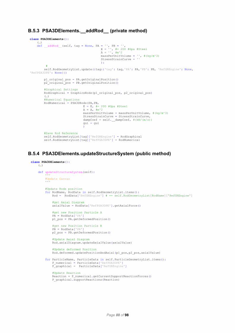
Page 88 of 98
B.5.3 PSA3DElements.__addRod__ (private method)
class PSA3DElements():
(…)
def __addRod__(self, tag = None, PA = '', PB = '',
E = '', #= 200 #Gpa #Steel
A = '', #m^2
massPerUnitVolume = '', #(kg/m^3)
StressStrainCurve = ''
):
#
self.RodGeometryList.update({tag:{'tag': tag,'PA': PA,'PB': PB, 'RefGREngine': None,
'RefPSA3DPE': None}})
p1_original_pos = PA.getOriginalPosition()
p2_original_pos = PB.getOriginalPosition()
#Graphical Settings
RodGraphical = GraphicsRods(p1_original_pos, p2_original_pos)
(…)
#Numerical Equations
RodNumerical = PSA3DRods(PA,PB,
E = E, #= 200 #Gpa #Steel
A = A, #m^2
massPerUnitVolume = massPerUnitVolume, #(kg/m^3)
StressStrainCurve = StressStrainCurve,
dampCoef = self.__dampCoef, #(kN/(m/s))
gui = gui
)
#Save Rod Reference
self.RodGeometryList[tag]['RefGREngine'] = RodGraphical
self.RodGeometryList[tag]['RefPSA3DPE'] = RodNumerical
B.5.4 PSA3DElements.updateStructureSystem (public method)
class PSA3DElements():
(…)
def updateStructureSystem(self):
"""
#Update Canvas
"""
#Update Rods position
for RodName, RodData in self.RodGeometryList.items():
Rod = RodData['RefGREngine'] # == self.RodGeometryList[RodName]['RefGREngine']
#get Axial Diagram
axialValue = RodData['RefPSA3DPE'].getAxialForce()
#get new Position Particle A
PA = RodData['PA']
p1_pos = PA.getDeformedPosition()
#get new Position Particle B
PB = RodData['PB']
p2_pos = PB.getDeformedPosition()
#Update Axial Diagram
Rod.axialDiagram.updateAxialValue(axialValue)
#Update deformed Position
Rod.deformed.updatePositionAndAxial(p1_pos,p2_pos,axialValue)
for ParticleName, ParticleData in self.ParticleGeometryList.items():
P_numerical = ParticleData['RefPSA3DPE']
P_graphical = ParticleData['RefGREngine']
#Update Reaction
Reaction = P_numerical.getCurrentSupportReactionForces()
P_graphical.supportReactions(Reaction)

Page 89 of 98
B.6 PSA3DPhysicsEngine
This section presents the classes related to the PSA3DPhysicsEngine, namely: PSA3DPhysicsEngine,
PSA3DRods, and PSA3DParticles.
B.6.1 PSA3DPhysicsEngine Numerical process
This section shows the implementation of the numerical process, presented in Figure 2.10 and
Figure 2.13. Notice that, Approach 2 has one more step, which consists of computing the kinetic energy
in each iteration.
class PSA3DPhysicsEngine():
(…)
def __numericalProcess__(self):
#Step 1 - Part 1
for ii, item in self.currentParticleGeometryList.items():
Pii = item['RefPSA3DPE']
Pii.numericalIntegration()
#Step 1 - Part 2 - Computing kinetic energy and execute Kinetic Damping Schema
if self.__kineticdampingschemeOPT == True:
#Computing kinetic energy
Uk_n_plus_1 = 0
for ii, item in self.currentParticleGeometryList.items():
Pii = item['RefPSA3DPE']
Uk_i = Pii.calculateKineticEnergy()
Uk_n_plus_1 = Uk_n_plus_1 + Uk_i
#Kinetic Damping Approach
#get Uk_n_less_1 and Uk_n
Uk_n_less_1 = self.Uk_n_less_1
Uk_n = self.Uk_n
#Check if it is a peak Kinetic Energy
if (Uk_n_less_1 <= Uk_n_plus_1) and (Uk_n <= Uk_n_plus_1):
#save Ec
self.Uk_n_less_1 = self.Uk_n
self.Uk_n = Uk_n_plus_1
itsPeak = False
else:
#Case - peak Kinetic Energy
for ii, item in self.currentParticleGeometryList.items():
Pii = item['RefPSA3DPE']
Pii.kineticDamping()
#Reset Ec
self.Uk_n_less_1 = 0
self.Uk_n = 0
itsPeak = True
#Step 2 - Calculate Rod's axial force
for ii, item in self.currentRodGeometryList.items():
Rii = item['RefPSA3DPE']
converge = Rii.calculateRodsAxialForce()
#Step 3 - check the stopping criterion
if converge == False: #Step 3b - Auxiliar, break if strain>>1!
print('\nDivergence results. Lower the value of damping coefficient and time-step!')
stoppingCriterionStatus = True
self.contador = 1000000
else:
FunbMax = 0
for ii, item in self.currentParticleGeometryList.items():
Pii = item['RefPSA3DPE']
Funb = Pii.checkStoppingCriterionStatus()
FunbMax = max(FunbMax,Funb)
if FunbMax <= self.tolerance:
stoppingCriterionStatus = True

Page 90 of 98
else:
stoppingCriterionStatus = False
#Step 3a - Is it a peak? Needs one more iteration!
if self.__kineticdampingschemeOPT == True:
if itsPeak == True:
stoppingCriterionStatus = False
return stoppingCriterionStatus
B.6.2 Approach 1
Approach 1 is implemented with two classes: PSA3DParticlesTrapezoidalRule and
PSA3DRodsSmallDisplacements.
B.6.2.1 PSA3DParticlesTrapezoidalRule
This section shows the implementation of the trapezoidal rule, presented before in Figure 2.11. class PSA3DParticlesTrapezoidalRule(PSA3DParticlesElementary):
def __init__(self,original_pos = [0,0,0],
constraint = [0,0,0],
FextGlobalAxis = [0,0,0],
appliedAccels = [0,0,0]
):
super(PSA3DParticlesArtificialDampingTrapezoidalRule, self).__init__(original_pos =
original_pos,
constraint = constraint,
FextGlobalAxis = FextGlobalAxis,
appliedAccels = appliedAccels
)
def __trapezoidalRuleFunction__(self, xn, vn, an, h):
#
vn1 = vn + an*h
xn1 = xn + (1/2)*h*(vn+vn1) #kN #Returns a row
return xn1, vn1
def __NumericalIntegration__(self):
#-------Numerical Method--------
#
xn = self.xn
vn = self.__vn
tn = self.tn
h = self.timeStep
#Trapezoidal rule
an = self.__computeAcceleration__( tn )
[xn1,vn1] = self.__trapezoidalRuleFunction__(xn, vn, an, h)
#Store results
self.tn += h #time t(n+1)
self.__vn = vn1 #Velocity in time t(n+1)
self.xn = xn1 #Position in time t(n+1)
return None

Page 91 of 98
B.6.2.2 PSA3DRodsSmallDisplacements
This section shows the implementation of the internal force calculation considering small displacements,
presented in Figure 2.12.
class PSA3DRodsSmallDisplacements(PSA3DRodsElementary):
def __init__(self, ParticleA = '', ParticleB = '',
E = None, #GPa #Steel
A = None, #m**2
massPerUnitVolume = None, #(kg/m^3)
StressStrainCurve = None,
dampCoef = None, #(kN/(m/s))
gui = False
):
super(PSA3DRodsSmallDisplacements, self).__init__(ParticleA = ParticleA, ParticleB =
ParticleB,
E = E, #GPa #Steel
A = A, #m**2
massPerUnitVolume = massPerUnitVolume, #(kg/m^3)
StressStrainCurve = StressStrainCurve,
gui = gui
)
self.__dampCoef = dampCoef
def __axialForce__(self):
'''
PSA3D Physics Engine by Paulo, Reydleon 2020 (20190528)
Calculates axial force
'''
#Compute the current length (Lk,n+1)
currentLength = self.__calculateCurrentLength__()
#Computed strain εk,n+1 = (Lk,n+1 - r)/r
strain = self.__calculateStrain__(self.restLength, currentLength)
#Calculate the internal force (fk,h = εk,n+1*E*A) on the local axis
Fint = self.Fint = self.__calculateInternalForce__(strain)
#Get velocity from the particles
v1 = self.ParticleA.getCurrentVelocity()
v2 = self.ParticleB.getCurrentVelocity()
#Calculate the damping force (fk,d) on the local axis
Fdmp = self.__calculateDampingForce__(v1,v2)
#Calculate the axial force (fk,n+1 = fk,h + fk,d)
Fa = Fint + Fdmp
#Compute the axial force (fk,n+1) on the global axis #(kN)
ForceAxialGlobal = LocalAxis2Global(self.T_Global2Local,tuple2NpArray([Fa,0,0]))
#(1x6 vector)
axialForceGlobal = set1x6SizeVector(ForceAxialGlobal, -ForceAxialGlobal)
#Store fk,n+1 for next iteration and save for graphical output
self.axialForceGlobal = axialForceGlobal
#Compute current Stress in MPa and save for graphical output
self.__computeCurrentStressAndAxialForce__(axialForceGlobal = axialForceGlobal,
currentTMatrix = self.T_Global2Local)
return self.converge

Page 92 of 98
B.6.3 Approach 2
Approach 2 is implemented with two classes: PSA3DParticlesKineticDamping and
PSA3DRodsLargeDisplacements.
B.6.3.1 PSA3DParticlesKineticDamping
This section shows the implementation of flow charts presented in Figure 2.14 and Figure 2.15. class PSA3DParticlesKineticDamping(PSA3DParticlesElementary):
def __init__(self,original_pos = [0,0,0],
constraint = [0,0,0],
FextGlobalAxis = [0,0,0],
appliedAccels = [0,0,0]
):
#NOTE: In the case of the Kinetic Damping the velocities are calculated in the midpoint
time (t = t+(1/2)Δt
super(PSA3DParticlesKineticDamping, self).__init__(original_pos = original_pos,
constraint = constraint,
FextGlobalAxis = FextGlobalAxis,
appliedAccels = appliedAccels
)
#set Auxiliary var
self.isPeak = True
def __NumericalIntegration__(self):
#-------Numerical Method--------
#
xn = self.xn
vn_less_f5 = self.vn_plus_f5
tn = self.tn
h = self.timeStep
#kinetic Damping
#Calculate acceleration
self.a_n = a_n = self.__computeAcceleration__(tn)
#Calculate velocity
if self.__isPeak == True:
#next iteration
vn_plus_f5 = (1/2)*h*a_n
#set Auxiliary var
self.__isPeak = False
else:
vn_plus_f5 = vn_less_f5 + h*a_n
#Calculate position
x_n_plus_1 = xn + h*vn_plus_f5 #m #Returns a row
#Store results
self.tn = self.tn + h #time t(n+1)
self.vn_plus_f5 = vn_plus_f5 #Velocity in time t(n+1)
self.xn = x_n_plus_1 #Position in time t(n+1)
return None

Page 93 of 98
B.6.3.2 PSA3DRodsLargeDisplacements
This section shows the implementation of the internal force calculation considering large displacements,
presented before in Figure 2.16.
class PSA3DRodsLargeDisplacements(PSA3DRodsElementary):
def __init__(self, ParticleA = '', ParticleB = '',
E = None, #GPa #Steel
A = None, #m**2
massPerUnitVolume = None, #(kg/m^3)
StressStrainCurve = None,
dampCoef = None, #(kN/(m/s))
gui = False
):
super(PSA3DRodsLargeDisplacements, self).__init__(ParticleA = ParticleA, ParticleB =
ParticleB,
E = E, #GPa #Steel
A = A, #m**2
massPerUnitVolume = massPerUnitVolume, #(kg/m^3)
StressStrainCurve = StressStrainCurve,
gui = gui
)
def __axialForce__(self):
'''
PSA3D Physics Engine by Paulo, Reydleon 2020 (20190528)
Calculates axial force
'''
#Last iteration
Ln = self.restLength
#Compute the current length (Lk,n+1), the Transformation Matrix and the rod unit vector
e1'2'
#(auxiliary step) get current position
posA = self.ParticleA.getDeformedPosition()
posB = self.ParticleB.getDeformedPosition()
#
Ln_1 = norm3D(posA,posB)
RodvectorGlobalUCS = posB - posA #tuple2NpArray
UnitVector, TMatrix = setTransformationMatrixGlobal2Local(RodvectorGlobalUCS) #Local to
global
#Computed strain εk,n+1 = (Lk,n+1 - Lk,n)/Lk,n
strain = self.__calculateStrain__(Ln,Ln_1)
#Calculate the internal force on the local axis
Fint = self.Fint = self.__calculateInternalForce__(strain)
#Compute the internal force (fk,n+1) on the global axis
#Global Axis #(kN) #Note E is in GPa and A in m**2. For that reason, E*A*10^6 == kN/m
ForceInternalGlobal = Fint*UnitVector #Global2LocalAxis
#(1x6 vector)
axialForceGlobal = set1x6SizeVector(ForceInternalGlobal, -ForceInternalGlobal)
#Calculate the current stress σk,n+1
currentStress = self.__computeCurrentStressAndAxialForce__(axialForceGlobal =
axialForceGlobal, currentTMatrix = TMatrix)
#Store Lk,n+1, fk,n+1 and σk,n+1 for next iteration
self.restLength = Ln_1
self.axialForceGlobal = axialForceGlobal
self.__LastStressMPa = currentStress
return self.converge

Page 94 of 98
B.7 Graphics Rendering Engine
This section presents the classes related to the Graphics Rendering Engine, namely: LineNodePath,
ElementaryLine, GraphicsParticles, and GraphicsRods.
B.7.1 LineNodePath
LineNodePath [88] is one of the basic drawing classes available in Panda3D. It inherits all the features
and properties of the NodePath class [73]. Some of the methods of this class are: drawLines, moveTo,
drawTo, reset, setColor, and create.
class LineNodePath(NodePath):
(…)
def __init__(self, parent = None, name = None,
thickness = 1.0, colorVec = VBase4(1)):
# Initialize the superclass
NodePath.__init__(self)
# Create a lineSegs object to hold the line
ls = self.lineSegs = LineSegs()
(…)
def drawLines(self, lineList):
"""
Given a list of lists of points, draw a separate line for each list
"""
for pointList in lineList:
self.moveTo(*pointList[0])
for point in pointList[1:]:
self.drawTo(*point)
(…)
def moveTo(self, *_args):
(…)
def drawTo(self, *_args):
(…)
def reset(self):
(…)
def setColor(self, *_args):
(…)
def create(self, frameAccurate = 0):
self.lineSegs.create(self.lineNode, frameAccurate)
The following script is an example of how to draw two lines and the result is shown in Figure 3.14.
import direct.directbase.DirectStart
from direct.directtools.DirectGeometry import LineNodePath
from pandac.PandaModules import Point3,Vec4
def drawLine(Name,p1 = (0,0,0),p2 = (0,0,0),Color = Vec4(0,0,0,0)):
#p1 and p2
arr_ = (p1[0],p1[1],p1[2]); p1 = Point3(arr_[0],arr_[1],arr_[2])
arr_ = (p2[0],p2[1],p2[2]); p2 = Point3(arr_[0],arr_[1],arr_[2])
rod = LineNodePath(render,Name,3,Color)
rod.moveTo(p1)
rod.drawTo(p2)
rod.create()
return rod
def main():
#Rod1
rod1 = drawLine(Name = 'Rod1', p1 = (0,0,0), p2 = (3,3,0), Color = Vec4(1,0,0,1))
#Rod2
rod2 = drawLine(Name = 'Rod2', p1 = (0,0,0), p2 = (4,3,0), Color = Vec4(0,0,1,0))
main()
run()

Page 95 of 98
B.7.2 ElementaryLine
This section introduces the constructor method of the ElementaryLine class. It inherits all the properties
and methods of the LineNodePath class (Annex B.7.1 and [88]). It receives as input the coordinates p1,
p2, the color and thickness.
class ElementaryLine(LineNodePath):
(…)
def __init__(self,p1,p2,strCOLOR = '',thickness = 3):
(…)
#Init
super().__init__( parent = None, name = '',
thickness = 3, colorVec = Vec4(0,0,0,0))
B.7.3 GraphicsParticles
The GraphicsParticles class is called whenever a particle is created. As explained in 3.5.1, the particle
element carries properties such as coordinates, nodal constraints, and external forces. The following
code presents the implementation of the graphical part of each particle.
class GraphicsParticles():
(…)
def __init__(self,originalPosition, constraints = [0,0,0],externalForce = [0,0,0]):
(…)
self.NodalConstraint = NodalConstraint(self.__originalPosition, self.__constraints)
self.ExternalForce = ExternalForce(self.__originalPosition, self.__externalForce,color =
'ColorBlue')
B.7.4 GraphicsRods
The GraphicsRods class is called whenever a rod is created. As explained in 3.5.2, the rod element is
organized into three classes, namely, ElementaryRod, AxialDiagram, and DeformedRod. Each rod
carries properties such as two particles that contain all their intrinsic properties, namely, original position,
deformed position, nodal constraints, and external forces. The following code presents the
implementation of the graphical part of each rod.
class GraphicsRods(ElementaryRod): (…)
def __init__(self,p1,p2,axialDiagramScale = 0.0, RodDeformedScale = 1.0 , strCOLOR =
'ColorBlack', thickness = 1.5):
#Converts to type (x,y,z)
p1 = (p1[0],p1[1],p1[2])
p2 = (p2[0],p2[1],p2[2])
#Rod
super().__init__(p1,p2,strCOLOR,thickness)
#Deformed Rod
self.deformed = DeformedRod(p1 = p1,p2 = p2, Scale = RodDeformedScale, strCOLOR =
'ColorBlue')
#Axial Diagram
self.axialDiagram = AxialDiagram(p1 = p1,p2 = p2, Scale = axialDiagramScale)

Page 96 of 98
B.8 Utils functions
Utils functions are a collection of small Python functions, which makes it easier to handle repetitive
tasks. It is divided into Matrix Operations and Transformation Functions.
B.8.1 matrixOperations
Matrix Operations functions are a collection of small Python functions based on the Python NumPy [67].
It makes it easier to handle the algebraic operations such as sum, addition, and product of vectors and
arrays. The resulting code can be summarized as: matrixLine2NPArray, tuple2Vec, getSize,
MatrixTranspose, Vecs2Matrix, matrixDot, isEqual, set1x6SizeVector, and multiplyAandB.
def __matrixLine2NPArray(vecMatrix):
"""
receive: tupleVec = matrix([x,y,z])
returns: array([x,y,z])
"""
def __tuple2Vec(tupleVec):
"""
receive: tupleVec = [1,2,3]
returns:
"""
def getSize(vecLine):
"""
receive:
a) vecLine = [48,54,60]
b) vecLine =
[[48]
[54]
[60]]
c) vecLine = Matrix
returns:
[numRows , numCols]
#see https://www.mathworks.com/help/matlab/ref/size.html
"""
def MatrixTranspose(MatrixM):
"""
receive:
MatrixM =
[[ 4 7 10]
[ 5 8 11]
[ 6 9 12]]
returns:
MatrixM =
[[ 4 5 6]
[ 7 8 9]
[ 10 11 12]]
"""
def Vecs2Matrix(a1,a2,a3):
"""
receive:
a1 = [4,5,6]
a2 = [7,8,9]
a3 = [10,11,12]
returns:
MatrixM =
[[ 4 5 6]
[ 7 8 9]
[ 10 11 12]]
"""
def matrixDot(MatrixM,vecT):

Page 97 of 98
"""
receive:
MatrixM =
[[ 4 7 10]
[ 5 8 11]
[ 6 9 12]]
vecT = [1 2 3]
vector line type Size = 1x3
returns:
vecRes = [48,54,60]
"""
def isEqual(v1,v2):
"""
Parameters: a1 ,a2 : array_like Input arrays.
returns: varBool: bool
Returns True if the arrays are equal
"""
def set1x6SizeVector(v1, v2):
"""
Parameters: v1 ,v2 : array_like
Input arrays.
returns: z3_: array_like
Outputs 1x6 array.
"""
def multiplyAandB(A,B):
"""
Parameters: z3: array_like
Outputs 1x6 arrays.
returns: z3: array_like
Outputs 1x3 array.
#See https://stackoverflow.com/questions/25573298/math-error-when-multiplying-float-by-
integer-in-python
"""

Page 98 of 98
B.8.2 TransformationFunctions
This section presents some relevant methods of the TransformationFunctions class, such as
setTransformationMatrixGlobal2Local, LocalAxis2Global, Global2LocalAxis, crossProduct, and
normalize3D.
def setTransformationMatrixGlobal2Local(RodvectorGlobalUCS):
'''
input:
RodvectorGlobalUCS = <e1,||RodvectorGlobalUCS||> = [x,y,z]
Receives a row 1x3 array
output:
principalAxisMatrix 3x3 = [e1,e2,e3]
example:
RodvectorGlobalUCS = [x y z] = [0, 0.8, 0.6]
TGlobal2Local = principalAxisMatrix 3x3 =
[[0.0 0.8 0.6]
[1.0 0.0 0.0]
[ 0 +0.6 -0.8]]
RodvectorGlobalUCS = [x y z] = [0, .5*sqrt(2), .5*sqrt(2)]
TGlobal2Local = principalAxisMatrix 3x3 =
[[0.0 .5*sqrt(2) .5*sqrt(2)]
[1.0 0.0 0.0]
[ 0 +.5*sqrt(2) -.5*sqrt(2)]]
'''
def LocalAxis2Global(TGlobal2Local, VlocalSectionAxis):
'''
Transform local Axis to Global
Return a column 3x1
'''
def Global2LocalAxis(TGlobal2Local,vGlobal):
'''
Transform Global Axis to local Axis
Return a column 3x1
'''
#----------------- AUXILIAR METHODS------------------
def __crossProduct(c1,c2):
'''
see https://www.mathworks.com/help/matlab/ref/cross.html
'''
def __normalize3D(vec):
'''
see https://www.mathworks.com/help/matlab/ref/cross.html
'''