An Integrative Model of Insect Flight Control

William B. Dickson∗

Andrew D. Straw∗

Christian Poelma∗

Michael H. Dickinson †

California Institute of Technology, 1200 E. California Boulevard, Pasadena, CA, 91125, US

This paper presents a framework for simulating the flight dynamics and control strategies

of the fruit fly Drosophila melanogaster. The framework consists of five main components;

an articulated rigid-body simulation, a model of the aerodynamic forces and moments, a

sensory systems model, a control model, and an environment model. In the rigid-body

simulation the fly is represented by a system of three rigid-bodies connected by a pair

of actuated ball-joints. At each instant of the simulation, the aerodynamic forces and

moments acting on the wings and body of the fly are calculated using an empirically derived

quasi-steady model. The pattern of wing kinematics is based on data captured from high-

speed video sequences. The forces and moments produced by the wings are modulated by

deforming the base wing kinematics along certain characteristic actuation modes. Models

of the fly’s visual and mechanosensory systems are used to generate inputs to a controller

that sets the magnitude of each actuation mode, thus modulating the forces produced by

the wings. This simulation framework provides quantitative test-bed for examining the

possible control strategies employed by flying insects. Examples demonstrating visual and

mechanosensory based pitch rate, velocity, altitude and flight speed control, as well as

visually guided flight down a tunnel, are presented.

I. Introduction

Flight, like all forms of locomotion, involves a complex interaction between an animal and its environment.Although neural circuits, muscles, and wings make up the central physical plant of an animal’s motor system,flight behavior does not result from a simple set of feed-forward commands. For example, most of an insect’snervous system is dedicated to the sensory information that is generated as the animal moves through itsenvironment.1 The insect’s brain rapidly processes and fuses this rich information stream to create a motorcode that can modify wing motion on a stroke by stroke basis.2 Sensory feedback is essential both for short-term stability as well as long-term guidance and navigation. What we view as behavior, such as a fly flittingacross the room to land on the window, represents the output of a complex set of sensory-motor circuits thatoperates through the dynamics of muscles, skeleton, aerodynamics forces, and the environment. Althoughbiologists have appreciated the central role of feedback in flight,3 conventional biological disciplines such asneurobiology or biomechanics are not endowed with the mathematical framework to deal with the feedbackin a rigorous manner. Fortunately, recent progress in insect aerodynamics has fostered new engineeringapproaches such as the application of control theory to animal flight.4, 5 Such work will be critical in furtherdeveloping an integrative view of flight biology, if for no other reason that it will provide a rigorous frameworkfor incorporating observations from multiple disciplines within a single context, as well as permit experimentsthat are not possible on a real animal. Indeed, the very nature of feedback dominated systems is that theyare robust to ablation and perturbation, a fact that renders them resistant to standard reductionist methods.

In this paper we present our first attempts at constructing a 3D dynamic model of the flight system ofa flying insect, the fruit fly, Drosophila melanogaster. Flies provide a convenient scaffold for an integratedcontrol model, because they have been subject to extensive investigations of aerodynamics, sensory process-ing, and motor control.6–22 In constructing this model, we target both short-term and long-terms goals.Immediately, we can ask if our understanding of fly aerodynamics, neurobiology, and biophysics is sufficient

∗Postdoctoral Scholar, Bioengineering, California Institute of Technology.†Esther M. and Abe M. Zarem Professor, Bioengineering, California Institute of Technology.

1 of 19

American Institute of Aeronautics and Astronautics

to create a simulated entity that can fly stably in a manner that captures some of the salient features ofa real fly. Towards this end, we must be careful not to bias our conclusions by deliberately choosing freeparameters that result in satisfactory performance but are not justified physiologically. The challenge hereis that certain features of our model are well constrained by detailed observation and experiment and easilyformulated (e.g. wing and body aerodynamics), while other components are poorly understood and may beonly roughly hewed in mathematical terms (e.g. neural circuitry and wing hinge mechanics). Despite thislimitation, we feel that enough is known regarding this particular organism to warrant such an attempt.The long-term goal, which is not contingent on immediate success, is to construct a model that will serveas a framework for future studies. As research on flight biology continues, black box simplifications thatare currently necessary will be replaced by more rigorous “bottom up” formulation, advancing both thepredictive power and physical reality of the model. The most satisfying result would be to create a usefulresearch tool that, in conjunction with experiments on real animals, provides new insight into the underlyingbiology.

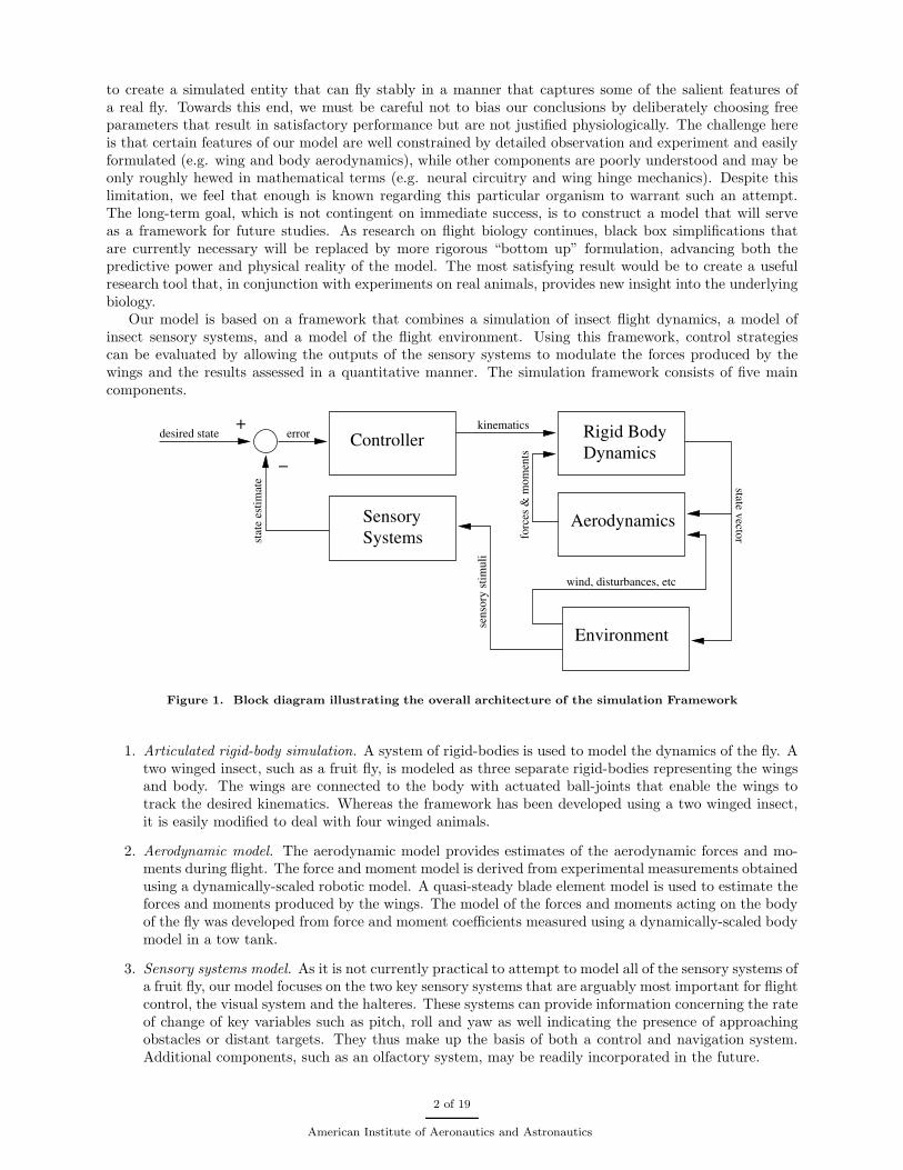
Our model is based on a framework that combines a simulation of insect flight dynamics, a model ofinsect sensory systems, and a model of the flight environment. Using this framework, control strategiescan be evaluated by allowing the outputs of the sensory systems to modulate the forces produced by thewings and the results assessed in a quantitative manner. The simulation framework consists of five maincomponents.

Sensory

−

+desired state error

Controller

wind, disturbances, etc

state vecto

r

kinematics

stat

e es

tim

ate

Aerodynamics

Rigid Body

Dynamics

Systems

Environment

senso

ry s

tim

uli

forc

es &

mom

ents

Figure 1. Block diagram illustrating the overall architecture of the simulation Framework

1. Articulated rigid-body simulation. A system of rigid-bodies is used to model the dynamics of the fly. Atwo winged insect, such as a fruit fly, is modeled as three separate rigid-bodies representing the wingsand body. The wings are connected to the body with actuated ball-joints that enable the wings totrack the desired kinematics. Whereas the framework has been developed using a two winged insect,it is easily modified to deal with four winged animals.

2. Aerodynamic model. The aerodynamic model provides estimates of the aerodynamic forces and mo-ments during flight. The force and moment model is derived from experimental measurements obtainedusing a dynamically-scaled robotic model. A quasi-steady blade element model is used to estimate theforces and moments produced by the wings. The model of the forces and moments acting on the bodyof the fly was developed from force and moment coefficients measured using a dynamically-scaled bodymodel in a tow tank.

3. Sensory systems model. As it is not currently practical to attempt to model all of the sensory systems ofa fruit fly, our model focuses on the two key sensory systems that are arguably most important for flightcontrol, the visual system and the halteres. These systems can provide information concerning the rateof change of key variables such as pitch, roll and yaw as well indicating the presence of approachingobstacles or distant targets. They thus make up the basis of both a control and navigation system.Additional components, such as an olfactory system, may be readily incorporated in the future.

2 of 19

American Institute of Aeronautics and Astronautics

4. Control model. The control model consists of a set of control laws specifying the behavior of the insectwith regard to sensory input. The control model provides a means by which the outputs of the sensorysystem modulate the wing kinematics thus providing actuation. Using this framework different controlstrategies can be systematically evaluated and compared with the results of laboratory experiments toprovide insight into insect flight control and behavior. Although the changes in wing motion generatedby the control model are based on observation of real flies20 the control model nevertheless representthe most coarsely rendered component of the model. No attempt was made, for example, to accuratelymodel neural circuitry or musculoskeletal dynamics.

5. Environment model. The environment model provides input to both the sensory systems and theaerodynamics model. By providing different visual information to the sensory organs, the environmentmodel enables us the flexibility of placing the insect in different virtual habitats, simulating both fieldand laboratory conditions. We can also add physical features such as wind gusts to provide realisticor arbitrary perturbations.

A schematic block diagram illustrating the interconnections between the components of the insect flightsimulation framework is shown in Figure 1.

II. Simulation Framework

The simulation framework consists of four separate software components encapsulating the aerodynamics,sensory, control, and environmental models. In addition the framework provides an Application ProgrammingInterface (API) through which the model parameters can be accessed and the interaction between the variouscomponents can specified. An overall goal is to provide a unified interface for rapidly developing insect flightmechanics and control simulations. In this section we briefly describe the models underlying the maincomponents of the simulation framework.

A. Articulated Rigid-Body Dynamics

The dynamics of the fly are provided by an articulated rigid-body simulation. Articulated rigid-body simu-lation is an extension of rigid-body simulation where the bodies are attached to each other using joints.23, 24

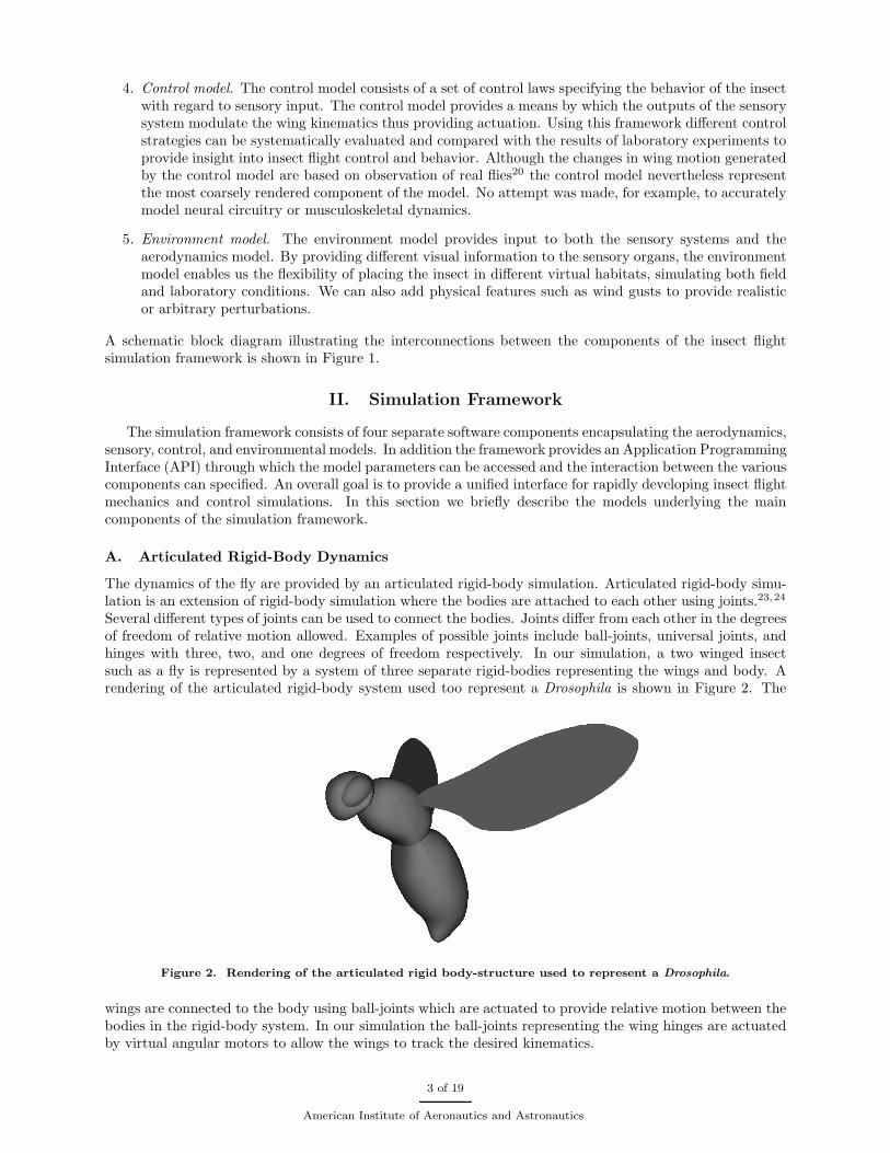
Several different types of joints can be used to connect the bodies. Joints differ from each other in the degreesof freedom of relative motion allowed. Examples of possible joints include ball-joints, universal joints, andhinges with three, two, and one degrees of freedom respectively. In our simulation, a two winged insectsuch as a fly is represented by a system of three separate rigid-bodies representing the wings and body. Arendering of the articulated rigid-body system used too represent a Drosophila is shown in Figure 2. The

Figure 2. Rendering of the articulated rigid body-structure used to represent a Drosophila.

wings are connected to the body using ball-joints which are actuated to provide relative motion between thebodies in the rigid-body system. In our simulation the ball-joints representing the wing hinges are actuatedby virtual angular motors to allow the wings to track the desired kinematics.

3 of 19

American Institute of Aeronautics and Astronautics

1. Physics Engine

At the heart of the articulated rigid-body simulation is a high performance physics library or physics engine.The physics engine provides a simulation of Newtonian physics for the rigid-body systems. For an introduc-tion to the mathematical methods used in physics engines and articulated rigid-body dynamics the readeris referred to Ref. 23 and Ref. 24. Physics engines are commonly used in the computer gaming industry fordeveloping interactive games as well as by the engineering community for studying manipulation and controlstrategies for robotic systems. For this reason there are many high quality physics engines available bothcommercially (Havok, Meqon, Novodex) and as open source software (Open Dynamics Engine, Dynamechs).

Several criteria were evaluated when selecting a physics engine for the project including the existenceusable API, good documentation, bindings to high level languages such as Python or Ruby, an active devel-oper community, and the availability of source code. Open Dynamics Engine (ODE) developed by RusselSmith and released under the LGPL open source license was found to be an excellent fit to these criteria.25

ODE is a full featured industrial quality physics engine which includes many advanced joint types, integratedcollision detection and a C/C++ API. Bindings to ODE are available in both Python and Ruby enablingrapid scripting using a high-level languages. In addition to several commercial computer games, ODE hasbeen used in both biomechanics and robotics research.26–28 The equations of motion for rigid-body systemsare derived from a Lagrange multiplier velocity based model.29

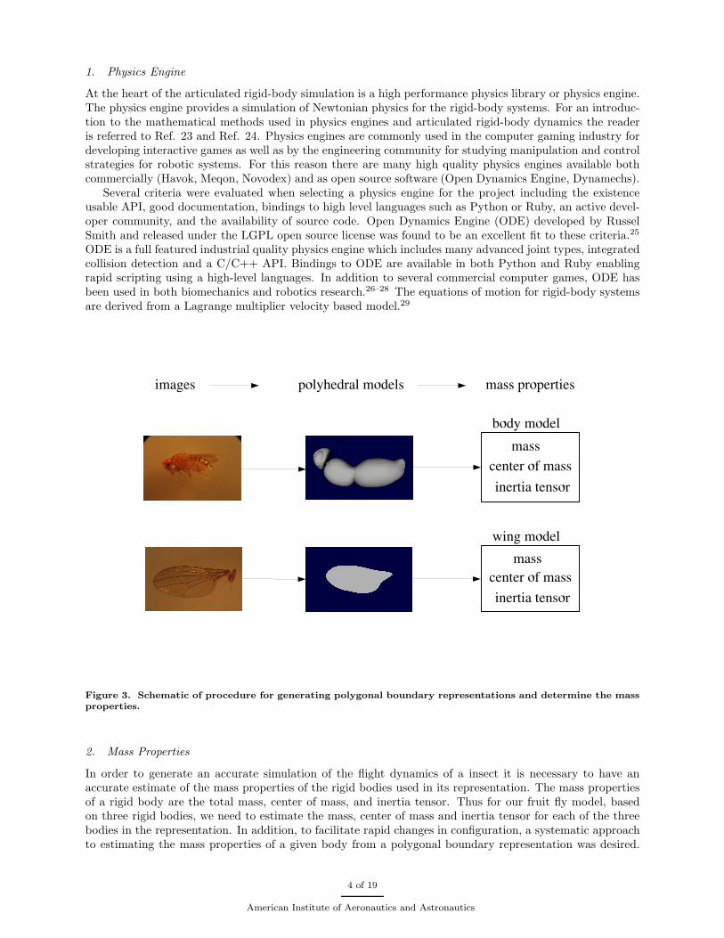
Figure 3. Schematic of procedure for generating polygonal boundary representations and determine the massproperties.

2. Mass Properties

In order to generate an accurate simulation of the flight dynamics of a insect it is necessary to have anaccurate estimate of the mass properties of the rigid bodies used in its representation. The mass propertiesof a rigid body are the total mass, center of mass, and inertia tensor. Thus for our fruit fly model, basedon three rigid bodies, we need to estimate the mass, center of mass and inertia tensor for each of the threebodies in the representation. In addition, to facilitate rapid changes in configuration, a systematic approachto estimating the mass properties of a given body from a polygonal boundary representation was desired.

4 of 19

American Institute of Aeronautics and Astronautics

Our basic strategy for generating polygonal models and estimating their mass properties is outlined below.

i.) Image Collection. Calibrated digital images of the object are collected from sufficient of vantage pointsto enable reconstruction of the object.

ii.) Boundary Model. Using the collected images a polygonal boundary representation of the object isdeveloped with a CAD program (e.g. SolidWorks) or 3D modeling software (e.g. Blender).

iii.) Mass Properties. From the polygonal boundary representation of the object and an estimate its densitythe mass properties are calculated using Mirtich’s algorithm.30

The use Mirtich’s algorithm restricts this approach to objects or bodies which have uniform density. Forthe Drosophila simulation all three rigid-bodies in the representation are assumed to have a uniform densityequal to that of water. This produces a mass value similar to those measured in real flies. A schematicoverview of the procedure outlined above is shown in Figure 3.

B. Aerodynamic Forces and Moments

The aerodynamic model is used to calculate the forces and moments acting on the body and wings of theinsect during flight. The model is quasi-steady and is based on empirically determined force and momentcoefficients. The quasi-steady assumption that is based on the observation the flow pattern and forces actingon a revolving wing display little time dependence even at angles of attack high enough to generate an leadingedge vortex.18, 31 The aerodynamics forces and moments generated by the wings and body are consideredseparately and it is assumed that they are not influenced by wing-wing and wing-body interactions.

1. Wing Aerodynamics

The wing aerodynamics model is based on prior work using a dynamically scaled physical model.16, 18, 19

In this model the wing is approximated by a flat plate with planform based on a Drosophila wing. Usinga standard blade element method, the wing is divided spanwise into a finite number of blade elements onwhich the forces and moments are calculated. The force on each blade element is calculated as the sum ofthe steady state, rotational, and added mass components

F = Fs + Fr + Fa. (1)

The total force on the acting on the wing is given by the sum of the blade element forces. However, in orderto generate the appropriate moments acting on the wing, the force produced by each blade element must beapplied to the rigid-body representing the wing in the appropriate location. This location for a given bladeelement is roughly approximated by mean spanwise location of the element and the chordwise position of thecenter of pressure for the element. The methods used for calculating the three force components in equation(1) as well for predicting the chordwise position of the center of pressure are summarized below.

The steady state component of the force acting on a blade element is convienently expressed in terms oflift and drag. The steady state lift and drag are proportional to the product of the air density ρ, the elementchord length c, the element width ∆r, and the square of the incident flow velocity in the plane of the bladeelement, ue. Note, the plane of the a blade element is defined as the subspace spanned by the wing normaland wing chord vectors that intersects the center line of the element. Expressions for the magnitudes of thesteady state lift and drag are given as follows

Fs,lift =1

2ρ c ||ue||2 CL(α)∆r and Fs,drag =

1

2ρ c ||ue||2 CD(α)∆r (2)

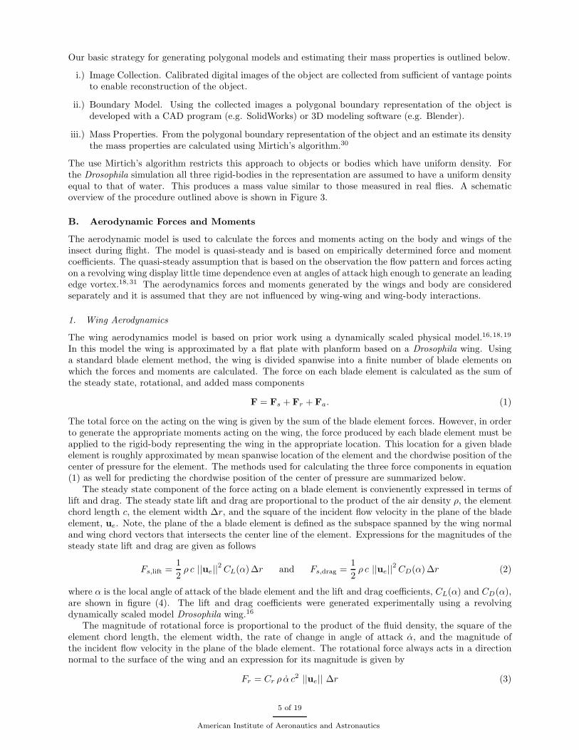
where α is the local angle of attack of the blade element and the lift and drag coefficients, CL(α) and CD(α),are shown in figure (4). The lift and drag coefficients were generated experimentally using a revolvingdynamically scaled model Drosophila wing.16

The magnitude of rotational force is proportional to the product of the fluid density, the square of theelement chord length, the element width, the rate of change in angle of attack α, and the magnitude ofthe incident flow velocity in the plane of the blade element. The rotational force always acts in a directionnormal to the surface of the wing and an expression for its magnitude is given by

Fr = Cr ρ α c2 ||ue|| ∆r (3)

5 of 19

American Institute of Aeronautics and Astronautics

Figure 4. Steady state lift (blue) and drag (red) coefficients for revolving model Drosophila wing.

where Cr is the rotational force coefficient. A value of Cr = 1.55 is suggested by Sane in Ref. 19 asappropriate for Drosophila wing. This value is essentially equivalent to the value derived by Fung32 usingthin airfoil theory and assuming that rotational axis of the wing is located at 1/4 chord.

The added mass force acting on a blade element is proportional to the density of the fluid, the square ofthe element chord length, the element width, and the acceleration of the incident flow normal to the surfaceof the element. The added mass force is assumed to always act normal to the surface of the wing. Anexpression for the magnitude of the added mass force is given by

Fa =ρπc2

4

{

ue · ue

||ue||sinα+ ||ue|| α cosα

}

∆r (4)

This estimate for the added mass force acting on blade element is based on an approximation for the motionsof an infinitesimally thin flat plate in an inviscid fluid, for example see Sedov.33

Measurements using a model Drosophila wing demonstrate that the spanwise location of the center ofpressure is approximately constant with respect changes angle of attack. This is in good agreement withpredictions by the quasi-steady model as shown in Figure 5(a).

An approximately linear relationship is found between angle of attack and the chordwise location of thecenter of pressure as shown in Figure 5(b). This linear relationship is well approximated by the followingequation

xcp(α) = c

[

0.82|α|π

+ 0.05

]

. (5)

In order to generate the appropriate moments acting on the entire wing, the force acting on each blade elementis applied at the spanwise location (or center) of the element and at the center of pressure determined byxcp(α) where α is the local angle of attack of the element.

2. Body Aerodynamics

The body aerodynamics model is used to calculate the forces and moments acting on the body of the insectduring flight. During the rigid-body simulation all the separately calculated body forces and moments areapplied at the center of mass of the insect’s body. The model assumes that the body of the insect is bilaterallysymmetric. Under this assumption the force and moment coefficients for the body are a function of the angleof attack of the body α, the sideslip angle β, and the Reynolds number (Re). In practice, the dependenceof force and moment coefficients on Re can be generally be ignored. This is due to the fact that variation

6 of 19

American Institute of Aeronautics and Astronautics

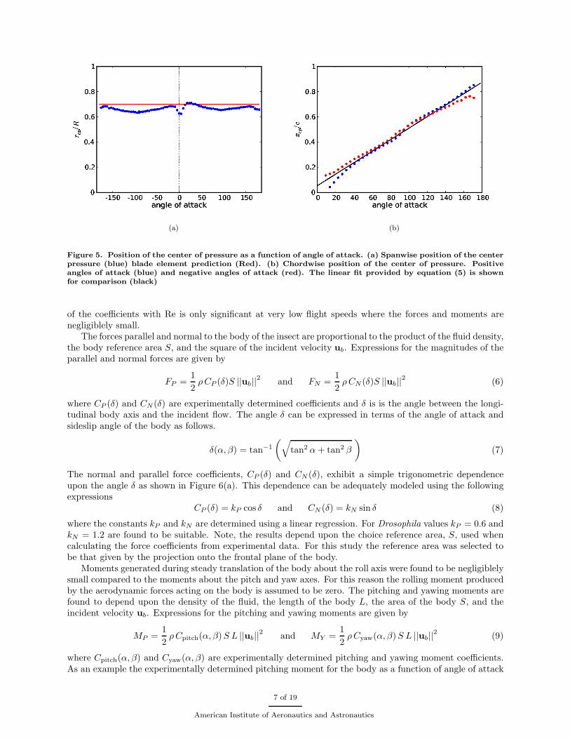
(a) (b)

Figure 5. Position of the center of pressure as a function of angle of attack. (a) Spanwise position of the centerpressure (blue) blade element prediction (Red). (b) Chordwise position of the center of pressure. Positiveangles of attack (blue) and negative angles of attack (red). The linear fit provided by equation (5) is shownfor comparison (black)

of the coefficients with Re is only significant at very low flight speeds where the forces and moments arenegligiblely small.

The forces parallel and normal to the body of the insect are proportional to the product of the fluid density,the body reference area S, and the square of the incident velocity ub. Expressions for the magnitudes of theparallel and normal forces are given by

FP =1

2ρCP (δ)S ||ub||2 and FN =

1

2ρCN (δ)S ||ub||2 (6)

where CP (δ) and CN (δ) are experimentally determined coefficients and δ is is the angle between the longi-tudinal body axis and the incident flow. The angle δ can be expressed in terms of the angle of attack andsideslip angle of the body as follows.

δ(α, β) = tan−1

(

√

tan2 α+ tan2 β

)

(7)

The normal and parallel force coefficients, CP (δ) and CN (δ), exhibit a simple trigonometric dependenceupon the angle δ as shown in Figure 6(a). This dependence can be adequately modeled using the followingexpressions

CP (δ) = kP cos δ and CN (δ) = kN sin δ (8)

where the constants kP and kN are determined using a linear regression. For Drosophila values kP = 0.6 andkN = 1.2 are found to be suitable. Note, the results depend upon the choice reference area, S, used whencalculating the force coefficients from experimental data. For this study the reference area was selected tobe that given by the projection onto the frontal plane of the body.

Moments generated during steady translation of the body about the roll axis were found to be negligiblelysmall compared to the moments about the pitch and yaw axes. For this reason the rolling moment producedby the aerodynamic forces acting on the body is assumed to be zero. The pitching and yawing moments arefound to depend upon the density of the fluid, the length of the body L, the area of the body S, and theincident velocity ub. Expressions for the pitching and yawing moments are given by

MP =1

2ρCpitch(α, β)S L ||ub||2 and MY =

1

2ρCyaw(α, β)S L ||ub||2 (9)

where Cpitch(α, β) and Cyaw(α, β) are experimentally determined pitching and yawing moment coefficients.As an example the experimentally determined pitching moment for the body as a function of angle of attack

7 of 19

American Institute of Aeronautics and Astronautics

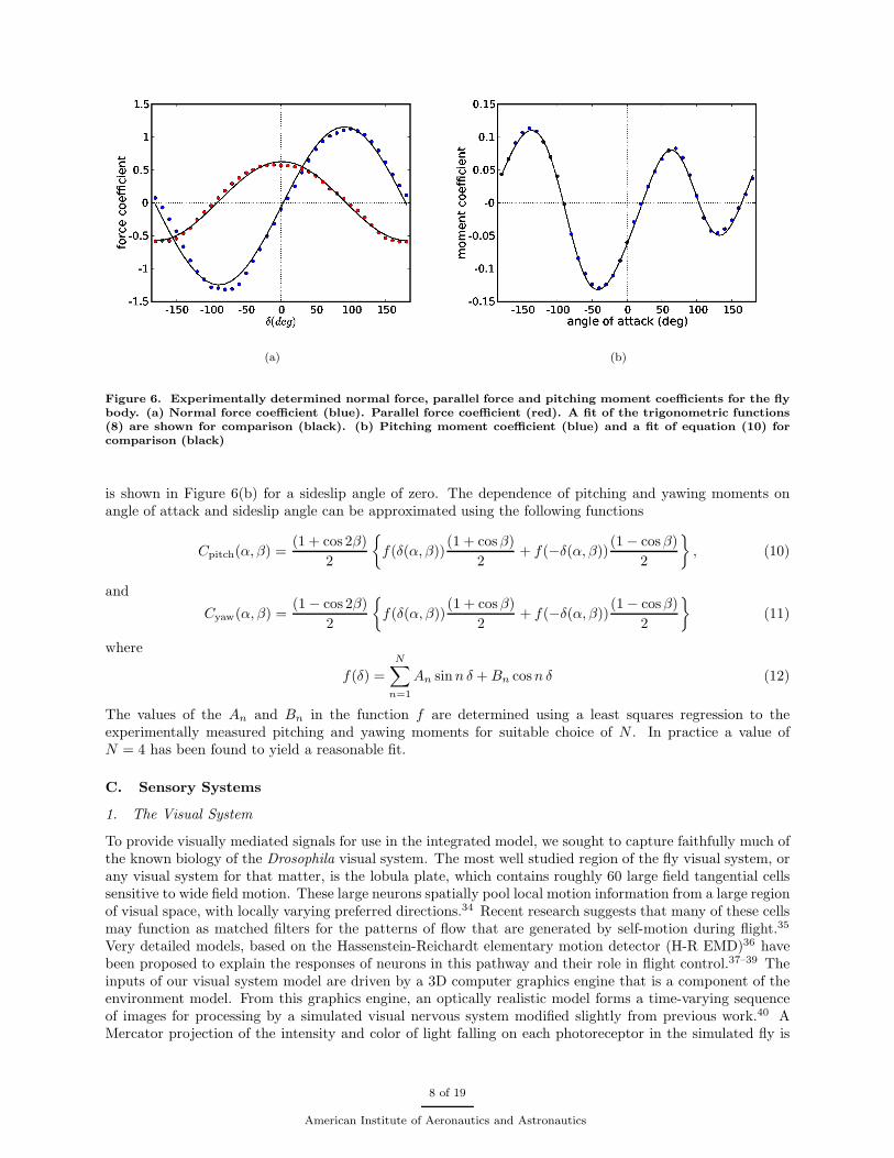
(a) (b)

Figure 6. Experimentally determined normal force, parallel force and pitching moment coefficients for the flybody. (a) Normal force coefficient (blue). Parallel force coefficient (red). A fit of the trigonometric functions(8) are shown for comparison (black). (b) Pitching moment coefficient (blue) and a fit of equation (10) forcomparison (black)

is shown in Figure 6(b) for a sideslip angle of zero. The dependence of pitching and yawing moments onangle of attack and sideslip angle can be approximated using the following functions

Cpitch(α, β) =(1 + cos 2β)

2

{

f(δ(α, β))(1 + cosβ)

2+ f(−δ(α, β))

(1 − cosβ)

2

}

, (10)

and

Cyaw(α, β) =(1 − cos 2β)

2

{

f(δ(α, β))(1 + cosβ)

2+ f(−δ(α, β))

(1 − cosβ)

2

}

(11)

where

f(δ) =

N∑

n=1

An sinn δ +Bn cosn δ (12)

The values of the An and Bn in the function f are determined using a least squares regression to theexperimentally measured pitching and yawing moments for suitable choice of N . In practice a value ofN = 4 has been found to yield a reasonable fit.

C. Sensory Systems

1. The Visual System

To provide visually mediated signals for use in the integrated model, we sought to capture faithfully much ofthe known biology of the Drosophila visual system. The most well studied region of the fly visual system, orany visual system for that matter, is the lobula plate, which contains roughly 60 large field tangential cellssensitive to wide field motion. These large neurons spatially pool local motion information from a large regionof visual space, with locally varying preferred directions.34 Recent research suggests that many of these cellsmay function as matched filters for the patterns of flow that are generated by self-motion during flight.35

Very detailed models, based on the Hassenstein-Reichardt elementary motion detector (H-R EMD)36 havebeen proposed to explain the responses of neurons in this pathway and their role in flight control.37–39 Theinputs of our visual system model are driven by a 3D computer graphics engine that is a component of theenvironment model. From this graphics engine, an optically realistic model forms a time-varying sequenceof images for processing by a simulated visual nervous system modified slightly from previous work.40 AMercator projection of the intensity and color of light falling on each photoreceptor in the simulated fly is

8 of 19

American Institute of Aeronautics and Astronautics

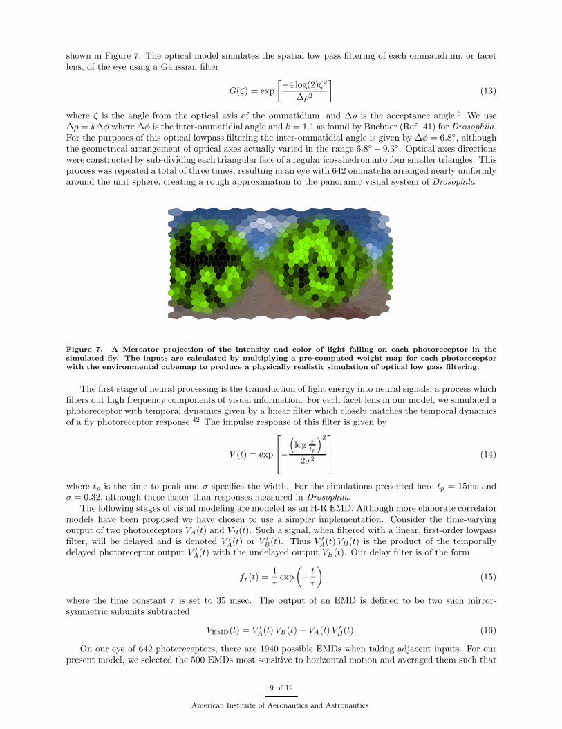
shown in Figure 7. The optical model simulates the spatial low pass filtering of each ommatidium, or facetlens, of the eye using a Gaussian filter

G(ζ) = exp

[−4 log(2)ζ2

∆ρ2

]

(13)

where ζ is the angle from the optical axis of the ommatidium, and ∆ρ is the acceptance angle.6 We use∆ρ = k∆φ where ∆φ is the inter-ommatidial angle and k = 1.1 as found by Buchner (Ref. 41) for Drosophila.For the purposes of this optical lowpass filtering the inter-ommatidial angle is given by ∆φ = 6.8◦, althoughthe geometrical arrangement of optical axes actually varied in the range 6.8◦ − 9.3◦. Optical axes directionswere constructed by sub-dividing each triangular face of a regular icosahedron into four smaller triangles. Thisprocess was repeated a total of three times, resulting in an eye with 642 ommatidia arranged nearly uniformlyaround the unit sphere, creating a rough approximation to the panoramic visual system of Drosophila.

Figure 7. A Mercator projection of the intensity and color of light falling on each photoreceptor in thesimulated fly. The inputs are calculated by multiplying a pre-computed weight map for each photoreceptorwith the environmental cubemap to produce a physically realistic simulation of optical low pass filtering.

The first stage of neural processing is the transduction of light energy into neural signals, a process whichfilters out high frequency components of visual information. For each facet lens in our model, we simulated aphotoreceptor with temporal dynamics given by a linear filter which closely matches the temporal dynamicsof a fly photoreceptor response.42 The impulse response of this filter is given by

V (t) = exp

−

(

log ttp

)2

2σ2

(14)

where tp is the time to peak and σ specifies the width. For the simulations presented here tp = 15ms andσ = 0.32, although these faster than responses measured in Drosophila.

The following stages of visual modeling are modeled as an H-R EMD. Although more elaborate correlatormodels have been proposed we have chosen to use a simpler implementation. Consider the time-varyingoutput of two photoreceptors VA(t) and VB(t). Such a signal, when filtered with a linear, first-order lowpassfilter, will be delayed and is denoted V ′

A(t) or V ′

B(t). Thus V ′

A(t)VB(t) is the product of the temporallydelayed photoreceptor output V ′

A(t) with the undelayed output VB(t). Our delay filter is of the form

fτ (t) =1

τexp

(

− t

τ

)

(15)

where the time constant τ is set to 35 msec. The output of an EMD is defined to be two such mirror-symmetric subunits subtracted

VEMD(t) = V ′

A(t)VB(t) − VA(t)V ′

B(t). (16)

On our eye of 642 photoreceptors, there are 1940 possible EMDs when taking adjacent inputs. For ourpresent model, we selected the 500 EMDs most sensitive to horizontal motion and averaged them such that

9 of 19

American Institute of Aeronautics and Astronautics

we had a single, wide-field motion sensitive neuron. We foresee implementing a more realistic network ofsimilar neurons in future models. We confirmed that the outputs of this neuron generate a strong outputsignal upon rotation and that the sign reversed when rotating in the opposite direction. Further the responseis near zero when there is equal and opposite optic flow on the two sides of the eye such as during forwardtranslation in the middle of a tunnel. Although flies have roughly 60 wide field cells in the lobula plate, ourpresent model incorporates only this single element.

2. The Halteres

In Diptera, including fruit flies, the pair of hindwings are modified into pair of dumb-bell shaped shapeorgans with a knob-like end and a stiff stalk. These organs are called halteres play an import role in flightstabilization. It has long been known that flies are unable to fly when their halteres are removed or immobi-lized.43 During flight the halteres oscillate in antiphase with the wings in planes that are tilted back from thesagital plane by approximately 30◦. The stalk of the haltere is heavily innervated with approximately 400mechanoreceptors.44–46 A subset of these mechanorecptors transduce information concerning the rotationalvelocity of the fly because they are exclusively sensitive the lateral deflections of the haltere within its strokeplane. Lateral forces are not caused by the back and forth beating of the haltere, but are generated byCoriolis forces caused by the angular rotation of the fly.47 An expression for the Coriolis force acting thehaltere of a fly during flight is given by

F = −2m (ω × v) (17)

where m is the mass of the haltere end knob, ω is the angular velocity of the fly, and v is the velocity of theend knob of the haltere relative to the fly.47 Note, a subscript L or R will be used when referring specificallyto left or right haltere respectively.

The haltere model assumes that the mass of the haltere is located in the end knob which is approximatedas a point mass. The angular position of the haltere within the stroke plane is given by the periodic functionψ(t) which is antiphase with the wing stroke position. The velocity of the left and right haltere end knobsrelative to the fly are given by

vL(t) =[

ψ(t) d cos θ sinψ(t), ψ(t) d cosψ(t), ψ(t) d sin θ sinψ(t)]T

(18)

and

vR(t) =[

−ψ(t) d cos θ sinψ(t), ψ(t) d cosψ(t), ψ(t) d sin θ sinψ(t)]T

(19)

respectively, where d is the length of the haltere and θ is the angle between the haltere stroke plane and thesagital plane. In this description the pitch, yaw, and roll axes of the fly are given by the x, y, and z bodyaxes respectively. The lateral components of the Coriolis forces acting on the left and right halters halteresare then given by

FL(t) = −2mψ(t) d [ωx(t) cos θ cosψ(t) − ωy(t) sinψ(t) + ωz(t) sin θ cosψ(t)] (20)

andFR(t) = −2mψ(t) d [ωx(t) cos θ cosψ(t) + ωy(t) sinψ(t) − ωz(t) sin θ cosψ(t)] (21)

respectively where ωx, ωy and ωz are the x, y and z components of the angular velocity vector. Fromequations (20) and (21) it is apparent that the Coriolis force acting on the haltere is complex waveformwhose value at any given instant depends upon the velocity of the haltere, the stoke position of the haltere,and the three components of the angular velocity vector.

A region of the haltere stalk, called the basal plate, contains numerous fields of companiform sensilla nearthe base of the haltere. One field in particular (dF2) is known to be particularly sensitive to lateral deflectionand is thought to act as the Coriolis detector.48 In this manner the fly is able to sense the lateral componentof the Coriolis forces. The neural processing of these signals is poorly understood. However, it is thoughtthat flies can sense all three components of the angular velocity vector using both of their halteres.49, 50 Inorder to use the halteres for sensory feedback in our integrated flight control model a scheme for convertingthe forces sensed by the halteres into changes in wing kinematics is required. As the neural processing bywhich this is done in the fruit fly is in general not well understood it is necessary for us posit a plausiblescheme instead. A first step in such a scheme is an estimate of the angular velocity from the Coriolis forces

10 of 19

American Institute of Aeronautics and Astronautics

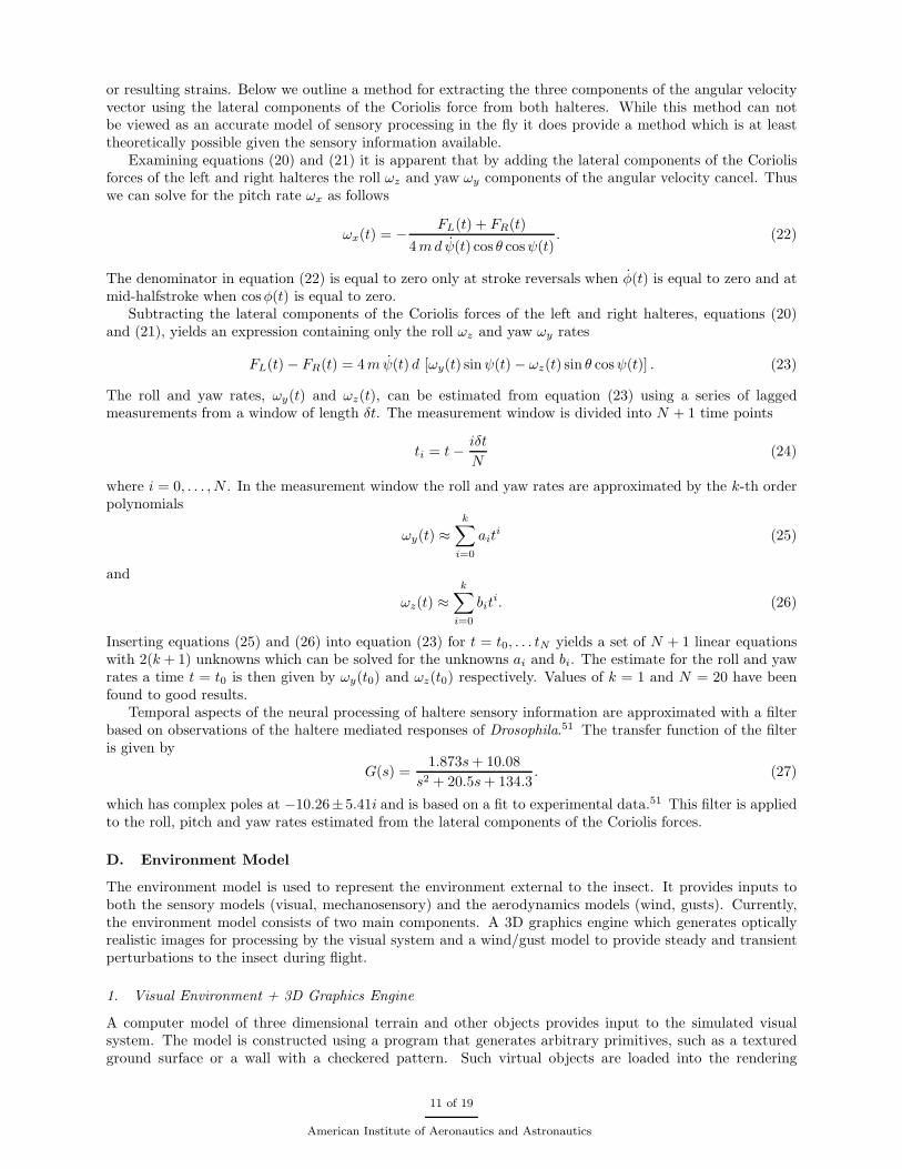
or resulting strains. Below we outline a method for extracting the three components of the angular velocityvector using the lateral components of the Coriolis force from both halteres. While this method can notbe viewed as an accurate model of sensory processing in the fly it does provide a method which is at leasttheoretically possible given the sensory information available.

Examining equations (20) and (21) it is apparent that by adding the lateral components of the Coriolisforces of the left and right halteres the roll ωz and yaw ωy components of the angular velocity cancel. Thuswe can solve for the pitch rate ωx as follows

ωx(t) = − FL(t) + FR(t)

4md ψ(t) cos θ cosψ(t). (22)

The denominator in equation (22) is equal to zero only at stroke reversals when φ(t) is equal to zero and atmid-halfstroke when cosφ(t) is equal to zero.

Subtracting the lateral components of the Coriolis forces of the left and right halteres, equations (20)and (21), yields an expression containing only the roll ωz and yaw ωy rates

FL(t) − FR(t) = 4mψ(t) d [ωy(t) sinψ(t) − ωz(t) sin θ cosψ(t)] . (23)

The roll and yaw rates, ωy(t) and ωz(t), can be estimated from equation (23) using a series of laggedmeasurements from a window of length δt. The measurement window is divided into N + 1 time points

ti = t− iδt

N(24)

where i = 0, . . . , N . In the measurement window the roll and yaw rates are approximated by the k-th orderpolynomials

ωy(t) ≈k

∑

i=0

aiti (25)

and

ωz(t) ≈k

∑

i=0

biti. (26)

Inserting equations (25) and (26) into equation (23) for t = t0, . . . tN yields a set of N + 1 linear equationswith 2(k + 1) unknowns which can be solved for the unknowns ai and bi. The estimate for the roll and yawrates a time t = t0 is then given by ωy(t0) and ωz(t0) respectively. Values of k = 1 and N = 20 have beenfound to good results.

Temporal aspects of the neural processing of haltere sensory information are approximated with a filterbased on observations of the haltere mediated responses of Drosophila.51 The transfer function of the filteris given by

G(s) =1.873s+ 10.08

s2 + 20.5s+ 134.3. (27)

which has complex poles at −10.26±5.41i and is based on a fit to experimental data.51 This filter is appliedto the roll, pitch and yaw rates estimated from the lateral components of the Coriolis forces.

D. Environment Model

The environment model is used to represent the environment external to the insect. It provides inputs toboth the sensory models (visual, mechanosensory) and the aerodynamics models (wind, gusts). Currently,the environment model consists of two main components. A 3D graphics engine which generates opticallyrealistic images for processing by the visual system and a wind/gust model to provide steady and transientperturbations to the insect during flight.

1. Visual Environment + 3D Graphics Engine

A computer model of three dimensional terrain and other objects provides input to the simulated visualsystem. The model is constructed using a program that generates arbitrary primitives, such as a texturedground surface or a wall with a checkered pattern. Such virtual objects are loaded into the rendering

11 of 19

American Institute of Aeronautics and Astronautics

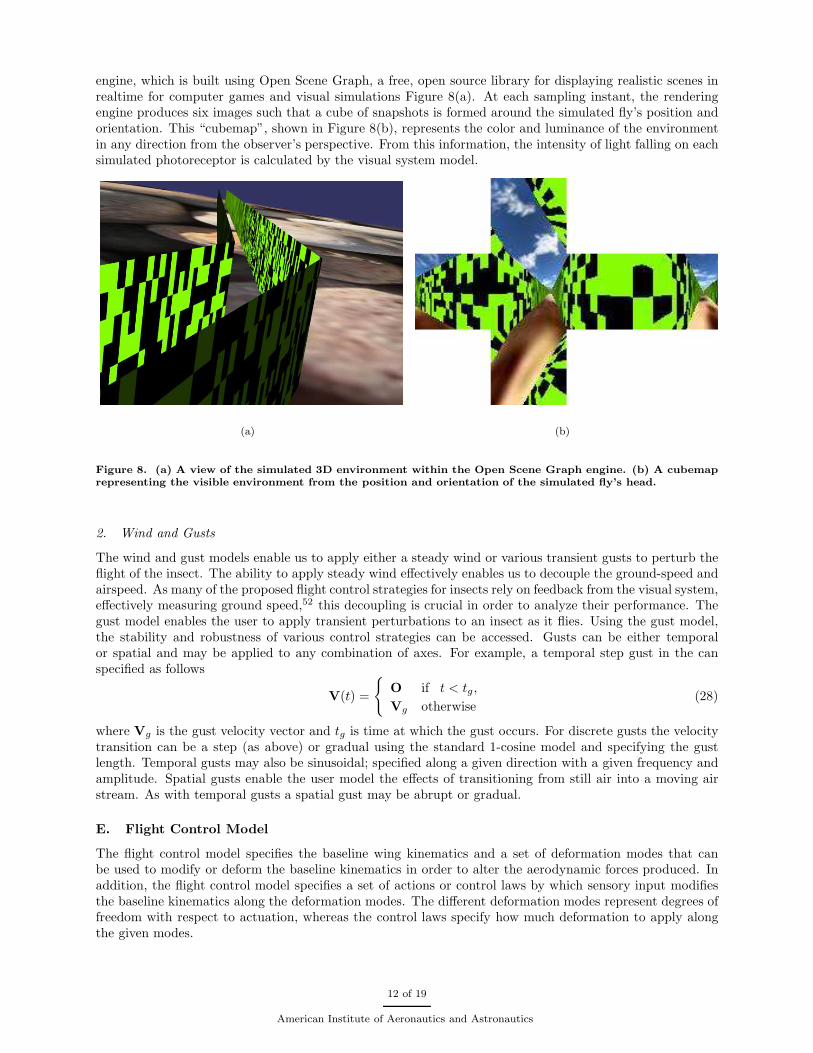
engine, which is built using Open Scene Graph, a free, open source library for displaying realistic scenes inrealtime for computer games and visual simulations Figure 8(a). At each sampling instant, the renderingengine produces six images such that a cube of snapshots is formed around the simulated fly’s position andorientation. This “cubemap”, shown in Figure 8(b), represents the color and luminance of the environmentin any direction from the observer’s perspective. From this information, the intensity of light falling on eachsimulated photoreceptor is calculated by the visual system model.

(a) (b)

Figure 8. (a) A view of the simulated 3D environment within the Open Scene Graph engine. (b) A cubemaprepresenting the visible environment from the position and orientation of the simulated fly’s head.

2. Wind and Gusts

The wind and gust models enable us to apply either a steady wind or various transient gusts to perturb theflight of the insect. The ability to apply steady wind effectively enables us to decouple the ground-speed andairspeed. As many of the proposed flight control strategies for insects rely on feedback from the visual system,effectively measuring ground speed,52 this decoupling is crucial in order to analyze their performance. Thegust model enables the user to apply transient perturbations to an insect as it flies. Using the gust model,the stability and robustness of various control strategies can be accessed. Gusts can be either temporalor spatial and may be applied to any combination of axes. For example, a temporal step gust in the canspecified as follows

V(t) =

{

O if t < tg,

Vg otherwise(28)

where Vg is the gust velocity vector and tg is time at which the gust occurs. For discrete gusts the velocitytransition can be a step (as above) or gradual using the standard 1-cosine model and specifying the gustlength. Temporal gusts may also be sinusoidal; specified along a given direction with a given frequency andamplitude. Spatial gusts enable the user model the effects of transitioning from still air into a moving airstream. As with temporal gusts a spatial gust may be abrupt or gradual.

E. Flight Control Model

The flight control model specifies the baseline wing kinematics and a set of deformation modes that canbe used to modify or deform the baseline kinematics in order to alter the aerodynamic forces produced. Inaddition, the flight control model specifies a set of actions or control laws by which sensory input modifiesthe baseline kinematics along the deformation modes. The different deformation modes represent degrees offreedom with respect to actuation, whereas the control laws specify how much deformation to apply alongthe given modes.

12 of 19

American Institute of Aeronautics and Astronautics

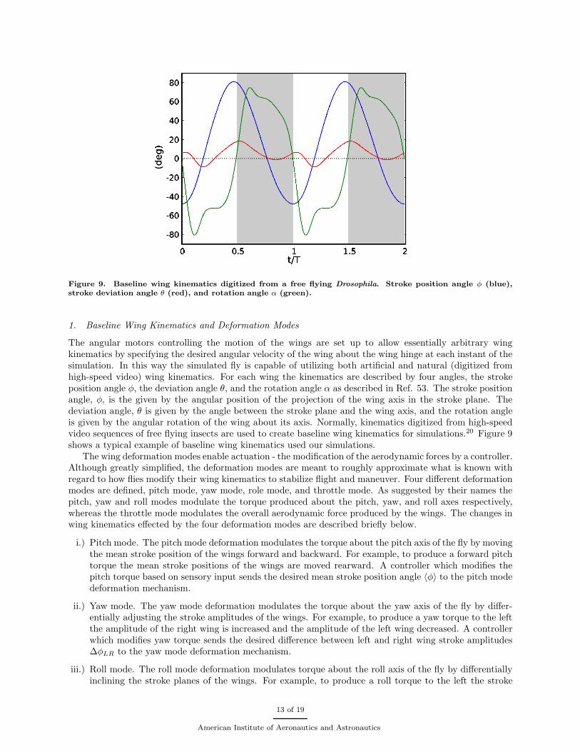
Figure 9. Baseline wing kinematics digitized from a free flying Drosophila. Stroke position angle φ (blue),stroke deviation angle θ (red), and rotation angle α (green).

1. Baseline Wing Kinematics and Deformation Modes

The angular motors controlling the motion of the wings are set up to allow essentially arbitrary wingkinematics by specifying the desired angular velocity of the wing about the wing hinge at each instant of thesimulation. In this way the simulated fly is capable of utilizing both artificial and natural (digitized fromhigh-speed video) wing kinematics. For each wing the kinematics are described by four angles, the strokeposition angle φ, the deviation angle θ, and the rotation angle α as described in Ref. 53. The stroke positionangle, φ, is the given by the angular position of the projection of the wing axis in the stroke plane. Thedeviation angle, θ is given by the angle between the stroke plane and the wing axis, and the rotation angleis given by the angular rotation of the wing about its axis. Normally, kinematics digitized from high-speedvideo sequences of free flying insects are used to create baseline wing kinematics for simulations.20 Figure 9shows a typical example of baseline wing kinematics used our simulations.

The wing deformation modes enable actuation - the modification of the aerodynamic forces by a controller.Although greatly simplified, the deformation modes are meant to roughly approximate what is known withregard to how flies modify their wing kinematics to stabilize flight and maneuver. Four different deformationmodes are defined, pitch mode, yaw mode, role mode, and throttle mode. As suggested by their names thepitch, yaw and roll modes modulate the torque produced about the pitch, yaw, and roll axes respectively,whereas the throttle mode modulates the overall aerodynamic force produced by the wings. The changes inwing kinematics effected by the four deformation modes are described briefly below.

i.) Pitch mode. The pitch mode deformation modulates the torque about the pitch axis of the fly by movingthe mean stroke position of the wings forward and backward. For example, to produce a forward pitchtorque the mean stroke positions of the wings are moved rearward. A controller which modifies thepitch torque based on sensory input sends the desired mean stroke position angle 〈φ〉 to the pitch modedeformation mechanism.

ii.) Yaw mode. The yaw mode deformation modulates the torque about the yaw axis of the fly by differ-entially adjusting the stroke amplitudes of the wings. For example, to produce a yaw torque to the leftthe amplitude of the right wing is increased and the amplitude of the left wing decreased. A controllerwhich modifies yaw torque sends the desired difference between left and right wing stroke amplitudes∆φLR to the yaw mode deformation mechanism.

iii.) Roll mode. The roll mode deformation modulates torque about the roll axis of the fly by differentiallyinclining the stroke planes of the wings. For example, to produce a roll torque to the left the stroke

13 of 19

American Institute of Aeronautics and Astronautics

plane of the right wing is inclined forward and stroke plane of the left wing is inclined rearward. Acontroller which modifies the roll torque sends the desired difference in stoke plane inclination ∆η tothe roll mode deformation mechanism.

iv.) Throttle mode. The throttle mode deformation modulates the overall aerodynamic force produced bythe wings by adjusting the wing beat frequency and stroke amplitude of both wings simultaneously.A controller that modifies the overall aerodynamic forces sends the desired change (from the baselinekinematics) in wing beat frequency ∆f and stroke amplitude ∆φ to the throttle mode deformationmechanism.

2. Angular Velocity Control

It is known that flies control angular velocity in compensatory manner, counter steering in response visual andmechanical stimulation.54 A basic control strategy developed for our framework emulates this by controllingthe angular velocity of the fly via a simple set of proportional controllers acting directly on the pitch, yawand roll deformation modes. Suppose the desired or set-point angular velocity vector is given by

ω∗ = (ω∗

x, ω∗

y , ω∗

z)T . (29)

In order to control the pitch rate, the input to the pitch mode deformation mechanism is set to valueproportional to the difference between the set-point pitch rate ω∗

x and the pitch rate as estimated from thehalteres ωx as follows

〈φ〉 = Gp (ω∗

x − ωx) (30)

where Gp is the gain of the controller. The difference in the set-point and estimated pitch rates is referredto as the pitch rate error. In a similar fashion the inputs to the yaw and roll deformation mechanisms areset to values proportional to the yaw rate and roll rate errors respectively

∆φLR = Gy

(

ω∗

y − ωy

)

and ∆η = Gr (ω∗

z − ωz) (31)

where Gy, and Gr are the gains of the controllers. This simple strategy produces a compensatory angularvelocity control similar to that seen in experiments54 when given set-point angular velocity where the pitch,yaw and roll rates are all equal to zero. In addition, by setting the angular velocity set-point to a nonzero ortime varying value, simple flight maneuvers can be effected. Figure 10 demonstrates tracking of a sinusoidallyvarying pitch rate command by this simple controller. The oscillations in pitch rate, seen in the figure, aredue to the time varying forces and torques produced by the flapping wings rather than instability in thecontroller.

3. Rate Based Velocity Control

Forward flight velocity in flies in known to be strongly correlated with the pitch angle of the body whichsuggests that forward velocity may be controlled by adjusting pitch or pitch rate.52 One control schemebeing tested using our framework employs this idea to control forward velocity using pitch rate. This isachieved by adjusting the pitch rate set-point of the angular velocity controller using the error between thedesired forward velocity v∗f and the perceived forward velocity vf as follows

ω∗

x = Gf,0

(

v∗f − vf

)

+Gf,1

(

v∗f − vf

)

(32)

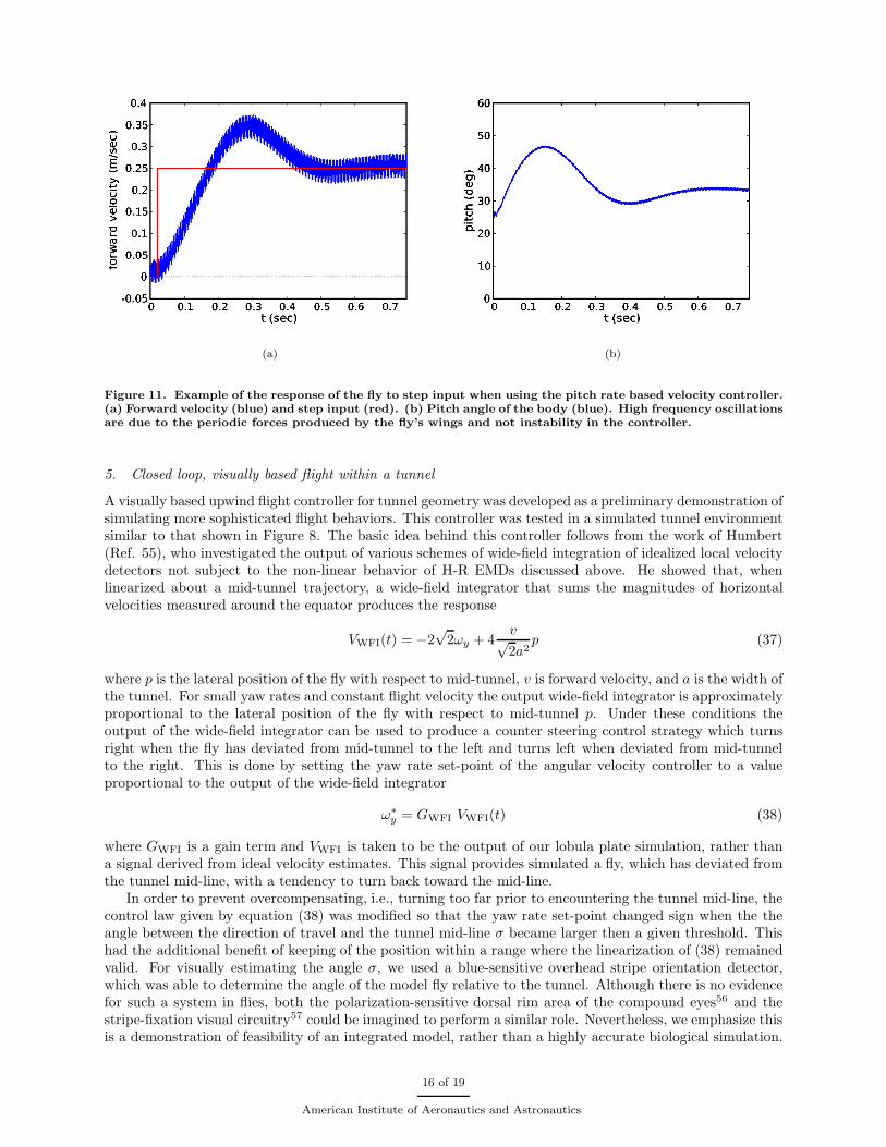
where the constants Gf,0 and Gf,1 are the controller gains. The first term in (32) is proportional to thevelocity error and the second is proportional to the derivative of the velocity error. The derivative term hasbeen found necessary to damp a stable limit cycle oscillation which occurs if only the proportional term isused. For a suitable choice of gains this controller has been found to yield stable forward flight at the desiredvelocity. In addition it provides pitch stability, effectively eliminating the slow drift in pitch that occurswhen only pitch rate control is used. The response of this controller to a step input in forward velocity isshown in Figure 11. In response to the step input the fly, initially at rest, pitches forward and accelerates. Itgains forward velocity and, as it approaches the set-point velocity, pitches back eventually reaching a stablepitch angle. The final pitch angle depends upon the set-point velocity in a manner similar to that found inexperiments with flies in a wind tunnel.52 Using an analogous controller the lateral velocity of the fly canalso be controlled by setting the yaw rate set-point using the error between the desired lateral velocity andthe perceived lateral velocity. Combining, these two control schemes gives a method by which the simulatedfly can perform simple maneuvers.

14 of 19

American Institute of Aeronautics and Astronautics

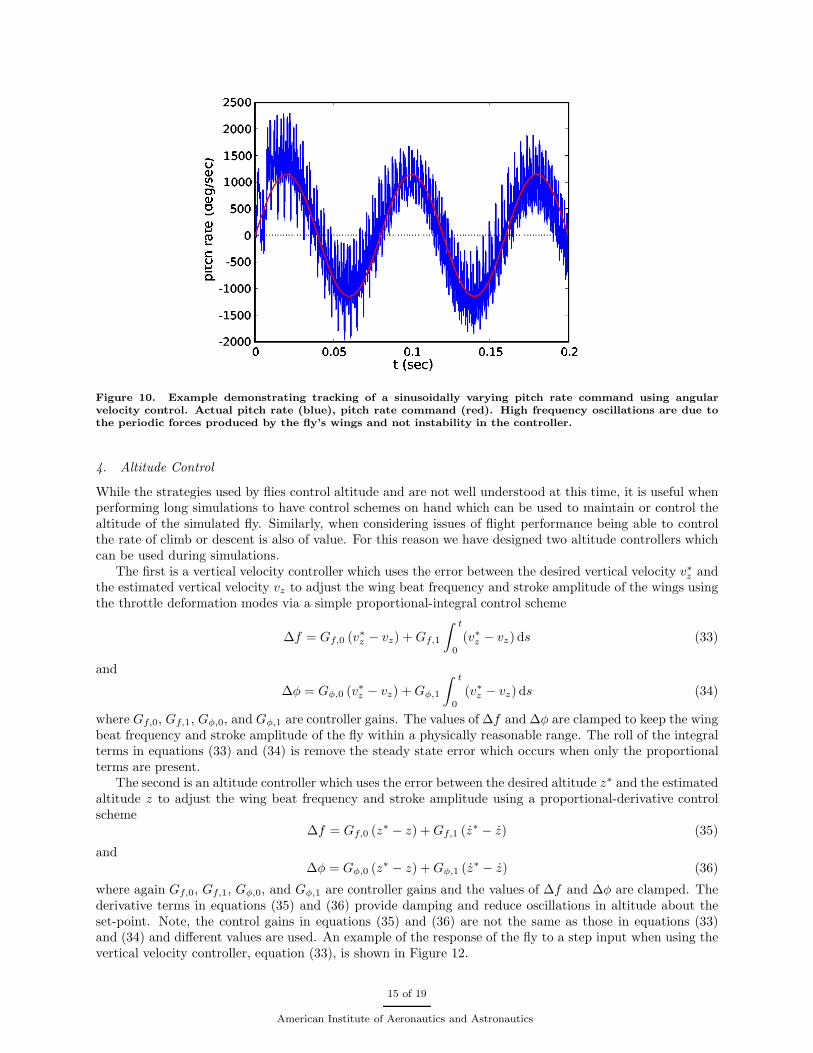
Figure 10. Example demonstrating tracking of a sinusoidally varying pitch rate command using angularvelocity control. Actual pitch rate (blue), pitch rate command (red). High frequency oscillations are due tothe periodic forces produced by the fly’s wings and not instability in the controller.

4. Altitude Control

While the strategies used by flies control altitude and are not well understood at this time, it is useful whenperforming long simulations to have control schemes on hand which can be used to maintain or control thealtitude of the simulated fly. Similarly, when considering issues of flight performance being able to controlthe rate of climb or descent is also of value. For this reason we have designed two altitude controllers whichcan be used during simulations.

The first is a vertical velocity controller which uses the error between the desired vertical velocity v∗z andthe estimated vertical velocity vz to adjust the wing beat frequency and stroke amplitude of the wings usingthe throttle deformation modes via a simple proportional-integral control scheme

∆f = Gf,0 (v∗z − vz) +Gf,1

∫ t

0

(v∗z − vz) ds (33)

and

∆φ = Gφ,0 (v∗z − vz) +Gφ,1

∫ t

0

(v∗z − vz) ds (34)

where Gf,0, Gf,1, Gφ,0, and Gφ,1 are controller gains. The values of ∆f and ∆φ are clamped to keep the wingbeat frequency and stroke amplitude of the fly within a physically reasonable range. The roll of the integralterms in equations (33) and (34) is remove the steady state error which occurs when only the proportionalterms are present.

The second is an altitude controller which uses the error between the desired altitude z∗ and the estimatedaltitude z to adjust the wing beat frequency and stroke amplitude using a proportional-derivative controlscheme

∆f = Gf,0 (z∗ − z) +Gf,1 (z∗ − z) (35)

and∆φ = Gφ,0 (z∗ − z) +Gφ,1 (z∗ − z) (36)

where again Gf,0, Gf,1, Gφ,0, and Gφ,1 are controller gains and the values of ∆f and ∆φ are clamped. Thederivative terms in equations (35) and (36) provide damping and reduce oscillations in altitude about theset-point. Note, the control gains in equations (35) and (36) are not the same as those in equations (33)and (34) and different values are used. An example of the response of the fly to a step input when using thevertical velocity controller, equation (33), is shown in Figure 12.

15 of 19

American Institute of Aeronautics and Astronautics

(a) (b)

Figure 11. Example of the response of the fly to step input when using the pitch rate based velocity controller.(a) Forward velocity (blue) and step input (red). (b) Pitch angle of the body (blue). High frequency oscillationsare due to the periodic forces produced by the fly’s wings and not instability in the controller.

5. Closed loop, visually based flight within a tunnel

A visually based upwind flight controller for tunnel geometry was developed as a preliminary demonstration ofsimulating more sophisticated flight behaviors. This controller was tested in a simulated tunnel environmentsimilar to that shown in Figure 8. The basic idea behind this controller follows from the work of Humbert(Ref. 55), who investigated the output of various schemes of wide-field integration of idealized local velocitydetectors not subject to the non-linear behavior of H-R EMDs discussed above. He showed that, whenlinearized about a mid-tunnel trajectory, a wide-field integrator that sums the magnitudes of horizontalvelocities measured around the equator produces the response

VWFI(t) = −2√

2ωy + 4v√2a2

p (37)

where p is the lateral position of the fly with respect to mid-tunnel, v is forward velocity, and a is the width ofthe tunnel. For small yaw rates and constant flight velocity the output wide-field integrator is approximatelyproportional to the lateral position of the fly with respect to mid-tunnel p. Under these conditions theoutput of the wide-field integrator can be used to produce a counter steering control strategy which turnsright when the fly has deviated from mid-tunnel to the left and turns left when deviated from mid-tunnelto the right. This is done by setting the yaw rate set-point of the angular velocity controller to a valueproportional to the output of the wide-field integrator

ω∗

y = GWFI VWFI(t) (38)

where GWFI is a gain term and VWFI is taken to be the output of our lobula plate simulation, rather thana signal derived from ideal velocity estimates. This signal provides simulated a fly, which has deviated fromthe tunnel mid-line, with a tendency to turn back toward the mid-line.

In order to prevent overcompensating, i.e., turning too far prior to encountering the tunnel mid-line, thecontrol law given by equation (38) was modified so that the yaw rate set-point changed sign when the theangle between the direction of travel and the tunnel mid-line σ became larger then a given threshold. Thishad the additional benefit of keeping of the position within a range where the linearization of (38) remainedvalid. For visually estimating the angle σ, we used a blue-sensitive overhead stripe orientation detector,which was able to determine the angle of the model fly relative to the tunnel. Although there is no evidencefor such a system in flies, both the polarization-sensitive dorsal rim area of the compound eyes56 and thestripe-fixation visual circuitry57 could be imagined to perform a similar role. Nevertheless, we emphasize thisis a demonstration of feasibility of an integrated model, rather than a highly accurate biological simulation.

16 of 19

American Institute of Aeronautics and Astronautics

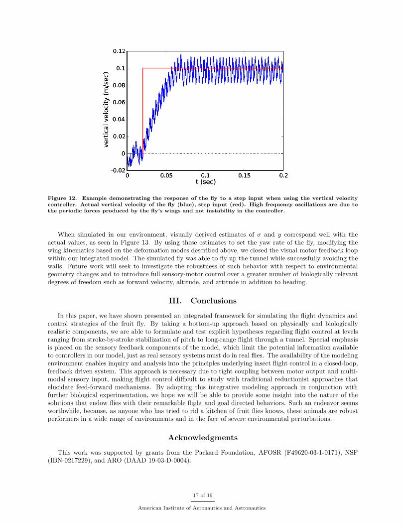
Figure 12. Example demonstrating the response of the fly to a step input when using the vertical velocitycontroller. Actual vertical velocity of the fly (blue), step input (red). High frequency oscillations are due tothe periodic forces produced by the fly’s wings and not instability in the controller.

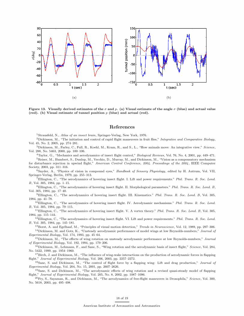
When simulated in our environment, visually derived estimates of σ and y correspond well with theactual values, as seen in Figure 13. By using these estimates to set the yaw rate of the fly, modifying thewing kinematics based on the deformation modes described above, we closed the visual-motor feedback loopwithin our integrated model. The simulated fly was able to fly up the tunnel while successfully avoiding thewalls. Future work will seek to investigate the robustness of such behavior with respect to environmentalgeometry changes and to introduce full sensory-motor control over a greater number of biologically relevantdegrees of freedom such as forward velocity, altitude, and attitude in addition to heading.

III. Conclusions

In this paper, we have shown presented an integrated framework for simulating the flight dynamics andcontrol strategies of the fruit fly. By taking a bottom-up approach based on physically and biologicallyrealistic components, we are able to formulate and test explicit hypotheses regarding flight control at levelsranging from stroke-by-stroke stabilization of pitch to long-range flight through a tunnel. Special emphasisis placed on the sensory feedback components of the model, which limit the potential information availableto controllers in our model, just as real sensory systems must do in real flies. The availability of the modelingenvironment enables inquiry and analysis into the principles underlying insect flight control in a closed-loop,feedback driven system. This approach is necessary due to tight coupling between motor output and multi-modal sensory input, making flight control difficult to study with traditional reductionist approaches thatelucidate feed-forward mechanisms. By adopting this integrative modeling approach in conjunction withfurther biological experimentation, we hope we will be able to provide some insight into the nature of thesolutions that endow flies with their remarkable flight and goal directed behaviors. Such an endeavor seemsworthwhile, because, as anyone who has tried to rid a kitchen of fruit flies knows, these animals are robustperformers in a wide range of environments and in the face of severe environmental perturbations.

Acknowledgments

This work was supported by grants from the Packard Foundation, AFOSR (F49620-03-1-0171), NSF(IBN-0217229), and ARO (DAAD 19-03-D-0004).

17 of 19

American Institute of Aeronautics and Astronautics

(a) (b)

Figure 13. Visually derived estimates of the σ and p. (a) Visual estimate of the angle σ (blue) and actual value(red). (b) Visual estimate of tunnel position p (blue) and actual (red).

References

1Strausfeld, N., Atlas of an insect brain, Springer-Verlag, New York, 1976.2Dickinson, M., “The initiation and control of rapid flight maneuvers in fruit flies,” Integrative and Comparative Biology ,

Vol. 45, No. 2, 2005, pp. 274–281.3Dickinson, M., Farley, C., Full, R., Koehl, M., Kram, R., and S., L., “How animals move: An integrative view,” Science,

Vol. 288, No. 5463, 2000, pp. 100–106.4Taylor, G., “Mechanics and aerodynamics of insect flight control,” Biological Reviews, Vol. 76, No. 4, 2001, pp. 449–471.5Reiser, M., Humbert, S., Dunlop, M., Vecchio, D., Murray, M., and Dickinson, M., “Vision as a compensatory mechanism

for disturbance rejection in upwind flight,” American Control Conference, 2004. Proceedings of the 2004 , IEEE ComputerSociety, 2003, pp. 311–316.

6Snyder, A., “Physics of vision in compound eyes,” Handbook of Sensory Physiology , edited by H. Autrum, Vol. VII,Springer-Verlag, Berlin, 1979, pp. 255–313.

7Ellington, C., “The aerodynamics of hovering insect flight. I. Lift and power requirements.” Phil. Trans. R. Soc. Lond.B , Vol. 305, 1984, pp. 1–15.

8Ellington, C., “The aerodynamics of hovering insect flight. II. Morphological parameters.” Phil. Trans. R. Soc. Lond. B ,Vol. 305, 1984, pp. 17–40.

9Ellington, C., “The aerodynamics of hovering insect flight. III. Kinematics.” Phil. Trans. R. Soc. Lond. B , Vol. 305,1984, pp. 41–78.

10Ellington, C., “The aerodynamics of hovering insect flight. IV. Aerodynamic mechanisms.” Phil. Trans. R. Soc. Lond.B , Vol. 305, 1984, pp. 79–115.

11Ellington, C., “The aerodynamics of hovering insect flight. V. A vortex theory.” Phil. Trans. R. Soc. Lond. B , Vol. 305,1984, pp. 115–144.

12Ellington, C., “The aerodynamics of hovering insect flight. VI. Lift and power requirements.” Phil. Trans. R. Soc. Lond.B , Vol. 305, 1984, pp. 145–181.

13Borst, A. and Egelhaaf, M., “Principles of visual motion detection,” Trends in Neuroscience, Vol. 12, 1989, pp. 297–306.14Dickinson, M. and Gotz, K., “Unsteady aerodynamic performance of model wings at low Reynolds-numbers,” Journal of

Experimental Biology , Vol. 174, 1993, pp. 45–64.15Dickinson, M., “The effects of wing rotation on unsteady aerodynamic performance at low Reynolds-numbers,” Journal

of Experimental Biology , Vol. 192, 1994, pp. 179–206.16Dickinson, M., Lehmann, F., and Sane, S., “Wing rotation and the aerodynamic basis of insect flight,” Science, Vol. 284,

No. 5422, 1999, pp. 1954–1960.17Birch, J. and Dickinson, M., “The influence of wing-wake interactions on the production of aerodynamic forces in flapping

flight.” Journal of Experimental Biology , Vol. 206, 2003, pp. 2257–2272.18Sane, S. and Dickinson, M., “The control of flight force by a flapping wing: Lift and drag production,” Journal of

Experimental Biology , Vol. 204, No. 15, 2001, pp. 2607–2626.19Sane, S. and Dickinson, M., “The aerodynamic effects of wing rotation and a revised quasi-steady model of flapping

flight,” Journal of Experimental Biology , Vol. 205, No. 8, 2002, pp. 1087–1096.20Fry, S., Sayaman, R., and Dickinson, M., “The aerodynamics of free-flight maneuvers in Drosophila,” Science, Vol. 300,

No. 5618, 2003, pp. 495–498.

18 of 19

American Institute of Aeronautics and Astronautics

21Birch, J., Dickson, W., and Dicksinson, M., “Force production and flow structure of the leading edge vortex on flappingwings at high and low Reynolds numbers.” Journal of Experimental Biology , Vol. 207, 2004, pp. 1063–1072.

22Dudley, R., The Biomechanics of Insect Flight , Princeton University Press, Princeton, New Jersey, 2000.23Shabana, A., Computational Dynamics, John Wiley and Sons Inc., New York, 2001.24Coutinho, M., Dynamic Simulations of Multibody Systems, Springer-Verlag, New York, 2001.25“http://www.ode.org/,” .26Durikovic, R. and Numata, K., “Human hand model based on rigid body dynamics,” IV ’04: Proceedings of the Infor-

mation Visualisation, Eighth International Conference on (IV’04), IEEE Computer Society, Washington, DC, USA, 2004, pp.853–857.

27Pollard, N. and Zordon, V., “Physically based grasping and control from example,” ACM SIGGRAPH / EurographicsSymposium on Computer Animation 2005 , Association for Computing Machinary, Inc., New York, 2005, pp. 311–358.

28Go, J., Browning, B., and Veloso, M., “Accurate and flexible simulation for dynamic, vision centric robots,” AutonomousAgents and Multiagent Systems (AAMAS 2004), IEEE Computer Society, New York, 2004, pp. 1386–1387.

29Stewart, D. and Trinkle, J., “An implicit time-stepping scheme for rigid body dynamics with inelastic collisions andCoulomb friction,” International J. Numer. Methods Engineering , Vol. 39, 1996, pp. 2673–2691.

30Mirtich, B., “fast and accurate computation of polyhedral mass properties,” Journal of Graphics Tools, Vol. 1, No. 2,1996.

31Birch, J. and Dickinson, M., “Spanwise flow and the attachment of the leading- edge vortex on insect wings.” Nature,Vol. 412, No. 6848, 2001, pp. 729–733.

32Fung, Y., An Introduction to the Theory of Aeroelasticity, New York: Dover, 1969.33Sedov, L., Two-Dimensional Problems in Hydrodynamics and Aerodynamics, Interscience Publishers, New York, 1965.34Hausen, K., “The lobula complex of the fly: Structure, function and significance in visual behavior,” Photoreception and

Vision in Invertebrates, edited by M. Ali, Plenum Press., New York, 1984, pp. 523–559.35Krapp, H. and Hengstenberg, R., “Estimation of self-motion by optic flow processing in single visual interneurons,”

Nature, Vol. 384, 1996, pp. 463–466.36Hassenstein, B. and Reichardt, W., “Systemtheoretische Analyse der Zeit-, Reihenfolgen- und Vorzeichenauswertung bei

der Bewegungsperzeption des Russelkafers Chlorophanus,” Zeitschrift Fur Naturforschung , Vol. 11b, 1956, pp. 513–524.37Egelhaaf, M., “Visual Afferences to Flight Steering Muscles Controlling Optomotor Responses of the Fly,” Journal of

Comparative Physiology A, Vol. 165, No. 6, 1989, pp. 719–730.38Shoemaker, P., O’Carroll, D., and Straw, A., “Velocity constancy and models for wide-field visual motion detection in

insects,” Biological Cybernetics, Vol. 93, No. 4, 2005, pp. 275–287.39Lindemann, J., Kern, R., van Hateren, J., Ritter, H., and Egelhaaf, M., “On the computations analyzing natural optic

flow: Quantitative model analysis of the blowfly motion vision pathway,” Journal of Neuroscience, Vol. 25, No. 27, 2005,pp. 6435–6448.

40Neumann, T., “Modeling insect compound eyes: Space-variant spherical vision,” Biologically Motivated Computer Vision,Proceedings, Vol. 2525, Springer-Verlag, Berlin, 2002, pp. 360–367.

41Buchner, E., “Behavioral analysis of spatial vision in insects,” Photoreception and vision in invertebrates, edited byM. Ali, Plenum Press., New York, 1984, pp. 561–621.

42Howard, J., Dubs, A., and Payne, R., “The dynamics of phototransduction in insects,” Journal of Comparative PhysiologyA, Vol. 154, 1984, pp. 707–718.

43Derham, W., “Boyle Lecture for 1711,” 1713.44Pflugsteadt, H., “Die Halteren der Dipteren,” Z. Wiss Zool., 1912, pp. 1–59.45Gnatzym, W., Grunert, U., and Bender, M., “Companoform sensilla of Calliphora vicina (Insecta Diptera) I. Topography,”

Zoomorphology , Vol. 106, 1987, pp. 312–319.46Hengstenberg, R., “Mechanosensory control of compensatory head rolling during flight in the blowfly Calliphora erythro-

cephala,” Meig. J. Comp. Physiol. A., Vol. 163, 1988, pp. 151–165.47Nalbach, G., “The Halteres of the blowfly Calliphora,” Journal of Comparative Physiology A, Vol. 173, 1994, pp. 293–300.48Fayyazuddin, A. and Dickinson, M., “Haltere afferents provide direct, electrotonic input to a steering motor neuron in

the blowfly Calliphora,” Journal of Neuroscience, Vol. 16, No. 16, 1996, pp. 5225–5232.49Faust, R., “Untersuchungen zum halterenproblem,” Zool. Jahrb. Physiol., Vol. 63, 1952, pp. 325–366.50Dickinson, M., “Haltere-mediated equilibrium reflexes of the fruit fly, Drosophila melanogaster,” Philos. Trans. R. Soc.

Lond., Vol. 354, No. 1385, 1999, pp. 903–916.51Sherman, A., The integration of visual and haltere feedback in Drosophila flight control , Ph.D. thesis, University of

California, Berkeley, 2003.52David, C., “Relationship between body angle and flight speed in free-flying Drosophila,” Physiological Entomology , Vol. 3,

No. 3, 1978, pp. 191–195.53Dickson, W. and Dickinson, M., “The effect of advance ratio on the aerodynamics of revolving wings,” Journal of

Experimental Biology , Vol. 207, 2004, pp. 4269–4281.54Sherman, A. and Dickinson, M., “Summation of visual and mechanosensory feedback in Drosophila flight control,” Journal

of Experimental Biology , Vol. 207, 2004, pp. 133–142.55Humbert, J., Bio-Inspired Visuomotor Convergence in Navigation and Flight Control Systems, Ph.D. thesis, California

Institute ofTechnology, 2005.56von Philipsborn, A. and Labhart, T., “A Behavioral-Study of Polarization Vision in the Fly, Musca-Domestica,” Journal

of Comparative Physiology a-Sensory Neural and Behavioral Physiology , Vol. 167, No. 6, 1990, pp. 737–743.57Gotz, K., “Course-Control, Metabolism and Wing Interference During Ultralong Tethered Flight in Drosophila-

Melanogaster,” Journal of Experimental Biology , Vol. 128, 1987, pp. 35–46.

19 of 19

American Institute of Aeronautics and Astronautics