Noname manuscript No.(will be inserted by the editor)

An Instantiation Scheme for Satisfiability Modulo Theories

Mnacho Echenim · Nicolas Peltier

May 2010

Abstract State-of-the-art theory solvers generally rely on an instantiation of the ax-

ioms of the theory, and depending on the solvers, this instantiation is more or less

explicit. This paper introduces a generic instantiation scheme for solving SMT prob-

lems, along with syntactic criteria to identify the classes of clauses for which it is

complete. The instantiation scheme itself is simple to implement, and we have pro-

duced an implementation of the syntactic criteria that guarantee a given set of clauses

can be safely instantiated. We used our implementation to test the completeness of our

scheme for several theories of interest in the SMT community, some of which are listed

in the last section of this paper.

1 Introduction

Most formal verification tools rely on procedures that decide the validity or, dually, the

satisfiability of logical formulas. In general, the considered formula (or set of clauses)

is ground and its validity needs only be tested modulo a background theory T . In

formal software verification for example, the background theory can define one or a

combination of data structures such as arrays or lists. These problems are known as T -

decision problems or more commonly, SMT problems, and the tools capable of solving

these problems are known as T -decision procedures, or SMT solvers (SMT stands for

Satisfiability Modulo Theories).

A lot of research has been devoted to the design of SMT solvers that are both

efficient and scalable. Generally, state-of-the-art SMT solvers rely on algorithms based

on the DPLL procedure [16,15] to deal with the boolean part of the SMT problems.

These solvers deal with the theory reasoning by applying methods ranging from the

eager approach, which consists in applying sophisticated techniques to reduce the entire

Mnacho EchenimUniversite de GrenobleE-mail: Mnacho.Echenim@imag.fr

Nicolas PeltierUniversite de Grenoble, CNRSE-mail: Nicolas.Peltier@imag.fr

2

SMT problem to an equisatisfiable SAT problem, to the lazy approach, which consists

in searching for a conjunction of literals satisfying the boolean part of the formula,

and testing whether this conjunction of literals is satisfiable modulo the background

theory. A survey on SMT solvers and the different approaches can be found in [6].

Quantifier reasoning is meant to tackle the issue of solving SMT problems with

formulas involving quantifiers. Most approaches rely on the original work of [21] on

the Simplify prover, in which heuristics for quantifier instantiation are devised. State-

of-the-art techniques include [25,18]. Of course, these heuristics are not complete in

general, and the class for which completeness is ensured is not precisely characterized.

Complete quantifier elimination can be efficiently performed for some particular the-

ories, such as linear arithmetic (see for instance [14]) or a subclass of the theory of

arrays [13].

The rewrite-based approach to solving SMT problems, initiated by [3], consists

in employing a theorem prover for first-order logic with equality to solve the SMT

problems. This approach is appealing, since by feeding any finitely axiomatized theory

along with a set of ground clauses, one obtains a system that is refutationally complete.

If the theorem prover is guaranteed to terminate on the input set, then it acts as a

decision procedure for the background theory. Thus, much research on this subject is

devoted to determining results on termination for the theorem prover [2,11,33,9]. The

main issue with the rewrite-based approach is that theorem provers are not designed to

handle the boolean part of a formula as efficiently as possible. Therefore, they do not

perform well on SMT problems with a large boolean part. A solution to this problem

consists in integrating the theorem prover with a DPLL-based tool, and although this

raises new issues, such an integration was accomplished in, e.g., [35,37,17].

Another solution to this problem was investigated in [10], which consists in decom-

posing the SMT problem into a definitional part, made up of a conjunction of ground

literals, and an operational part, containing the boolean structure of the problem. Dur-

ing the first stage, the theorem prover is fed the definitional part of the SMT problem

along with the background theory, and the saturation process compiles the theory

away. During the second stage, the saturated set generated by the theorem prover is

fed to a DPLL-based tool, along with the operational part of the SMT problem. This

approach allows to exploit the full power of the theorem prover and the DPLL-based

tool, without requiring a tight integration between them. However, in the theory of

arrays for example, the set of clauses obtained after compiling the theory away is not

ground, and requires an additional instantiation before being fed to the DPLL-based

tool.

The goal of this paper is to investigate how the instantiation phases of the saturation

process can be singled out in order to devise a generic instantiation scheme for solving

SMT problems. Solving an SMT problem modulo a background theory for which the

instantiation scheme is complete would thus reduce to testing the satisfiability of a

ground formula in first-order logic with equality, with no mention to any background

theory. This scheme is meant to be as efficient as possible, i.e., instantiate the non-

ground clauses under consideration as little as possible.

This approach is close to that of [13] for the theory of arrays. However, contrary to

that of [13] which is model-theoretic, this one is proof-theoretic, and is not restricted

to just one theory or its extensions. The efficiency requirement comes at the expense

of completeness, and contrary to the schemes of [24,34,28], it is not always guaranteed

that the original set of clauses and the instantiated one are equisatisfiable. However,

3

the class of theories for which the scheme is complete is large enough to capture several

theories of interest in the SMT community.

This paper presents the instantiation scheme that was devised, along with two sets

of syntactic criteria on clauses, that guarantee the instantiated set of clauses and the

original one are equisatisfiable. The first set of criteria is simpler to implement, and

the other is more general. The imposed conditions have a common characteristic: they

are based on syntactic properties of the arguments of function symbols. Depending on

their positions, the former may be required to be ground, or to have a limited depth.

These conditions come up quite naturally in our proof-theoretic setting, and are general

enough for many theories of data structures from SMT problems to comply by them.

These criteria have been implemented1, and have allowed us to verify automatically

that the instantiation scheme can be applied to several theories such as arrays, records

or lists.

The rest of the paper is organized as follows.

– Section 2 reviews some usual definitions and basic results on equational clausal logic

and superposition-based theorem proving. Most definitions are standard although

we introduce some additional notations that are useful in our context. We also

introduce two classes of terms that play a central role in the paper: the classes of

I0-flat and Inv-closed terms, and several properties of these classes are proven.

– In Section 3 a new instantiation scheme is devised which reduces a set of first-

order clauses S to a set of ground instances Sλ. Sλ is always finite, which implies

that, in contrast to other approaches (e.g. [32,34,24]), our instantiation scheme

is not complete (S and Sλ are not always equisatisfiable). Some simple semantic

conditions are proposed in order to ensure completeness. These conditions are proof-

theoretic: the instantiation scheme is complete if S admits a particular kind of

refutation, called a simple refutation. Clause sets admitting simple refutations are

called simply provable clause sets.

– In Section 4 we introduce the syntactic class of so-called controlled clause sets, and

we prove that they are always simply provable, which implies that the satisfiability

problem is decidable for controlled sets.

– Controlled clause sets are not expressive enough to include usual theories of interest

such as the theory of arrays. Section 5 shows that the conditions of Section 4 can

be relaxed to handle a larger class of theories. The basic idea is that we only

need to ensure that the relevant consequences of the considered clause set will be

controlled, even if the parent clauses are not controlled. The clause sets satisfying

these conditions are called controllable clause sets.

– Section 6 contains examples of controllable theories (including all the theories that

can be handled by the superposition-based approach), additional algorithms and

practical remarks.

– Finally, Section 7 concludes the paper.

Due to the length of the paper, some of the proofs (in particular the most technical

ones) have been shifted to the appendix in order to improve readability. Also, our

results extend in a straightforward manner to a many-sorted framework, but we have

chosen to present them in a single-sorted framework for the sake of clarity.

1 http://membres-lig.imag.fr/peltier/fish.html

4

2 Preliminaries

2.1 Basic definitions

In this section we briefly review some usual definitions and notations in Logic and

Automated Theorem Proving. The results are standard and their proofs are omitted;

we refer the reader to, e.g., [5,4] for details.

We assume given a set of variables V, a set of function symbols Σ (containing at

least a constant symbol) and an arity function mapping each element of Σ to a natural

number. Σn denotes the set of symbols of arity n in Σ. Throughout this paper, a, b, c

always denote constant symbols, f, g, h denote function symbols and x, y, z denote

variables (possibly with indices). The symbol true denotes a special constant symbol

used to encode predicate symbols.

The sets of terms, atoms, literals and clauses are defined in the standard way on

Σ and V, using the equality symbol ≃. The notions of interpretations, models and

satisfiability are defined as usual. Two sets of clauses S, S′ are equisatisfiable if either

S, S′ are both unsatisfiable or S, S′ are both satisfiable.

A substitution is a function mapping every variable to a term. The set of variables

x such that xσ 6= x is called the domain of σ and denoted by dom(σ). A substitution

σ of domain x1, . . . , xn such that xiσ = ti for i = 1, . . . , n is usually denoted by

{xi 7→ ti | i ∈ [1..n]}. As usual, a substitution can be extended into a homomorphism

on terms, atoms, literals and clauses. The image of an expression e by a substitution σ

will be denoted by eσ. If E is a set of expressions, then Eσ denotes the set {eσ | e ∈ E}.The composition of two substitutions σ and θ is denoted by σθ. A substitution σ is

more general than θ if there exists a substitution η such that θ = ση. The substitution

σ is a renaming if it is injective and ∀x ∈ dom(σ), xσ ∈ V; and it is a unifier of two

terms t, s if tσ = sσ. Any unifiable pair of terms (t, s) has a most general unifier, unique

up to a renaming, and denoted by mgu(t, s). A term or clause containing no variable is

ground. A substitution σ is ground if xσ is ground, for every variable x in its domain.

A position is a finite sequence of natural numbers. ǫ denotes the empty se-

quence and p.q denotes the concatenation of p and q. p is a position in t if either

p = ǫ or p = i.q, t = f(t1, . . . , tn) and q is a position in ti. t|p and t[s]p re-

spectively denote the subterm at position p in t and the term obtained by replac-

ing the term at position p by s: t|ǫdef

= t, f(t1, . . . , tn)|i.qdef

= ti|q , t[s]ǫdef

= s and

f(t1, . . . , tn)[s]i.qdef

= f(t1, . . . , ti−1, ti[s]q , ti+1, . . . , tn). These notions extend straight-

forwardly to atoms, literals or clauses.

Flatness

A term is flat if it is a variable or a constant symbol. The set of flat terms is denoted

by T0: T0def

= V ∪Σ0. A non-flat term is complex. A clause C is flat2 if for every literal

t ≃ s or t 6≃ s occurring in C, t, s ∈ T0. A substitution σ is flat if ∀x ∈ V, xσ ∈ T0. A

clause C is a flat instance of D if there exists a flat substitution σ such that C = Dσ;

note that C is not necessarily flat. Flat substitutions are stable by composition:

Proposition 1 Let σ and µ be flat substitutions. Then σµ is also flat.

2 Note that we depart from the definition of, e.g., [3], where a flat literal can be of the formf(a1, . . . , an) ≃ b for some flat terms a1, . . . , an, b ∈ T0.

5

Any set of ground clauses can be flattened, by introducing fresh constants that serve

as names for complex terms. This operation produces a set of ground clauses such that

the only non-flat clauses are of the form f(a1, . . . , an) ≃ b, for constants a1, . . . , an, b.

For example, S = {f(a) 6≃ f(c)∨a ≃ c, f(b) 6≃ f(c)∨b ≃ c} is flattened by introducing

the fresh constants a′, b′ and c′, and replacing S by

{f(a) ≃ a′, f(b) ≃ b′, f(c) ≃ c′, a′ 6≃ c′ ∨ a ≃ c, b′ 6≃ c′ ∨ b ≃ c}.

The original set of ground clauses and the flattened one are equisatisfiable.

2.2 Superposition

We review some basic notions about superposition-based theorem proving, following

the formalism of [5].

Selection and Inference

Let < denote a reduction ordering which is substitution-monotonic (i.e. for every σ,

(t < s) ⇒ (tσ < sσ)). We assume that if a is a constant and t is a complex term,

then a < t. This property on orderings is termed as the goodness property in [2]. The

ordering < is extended to atoms, literals and clauses using the multiset extension. A

literal L is maximal in a clause C if for every L′ ∈ C, L 6< L′.

We consider a selection function sel which maps every clause C to a set of selected

literals in C. A term t is eligible in a clause C if t is not a variable and there exist two

terms u, v such that u 6< v, t occurs in u and sel(C) contains either u ≃ v or u 6≃ v.

Definition 1 A clause C is variable-eligible if sel(C) contains a literal of the form

x ≃ t or x 6≃ t, where x ∈ V and x 6< t.

For example, assume that sel(C) is the set of maximal literals in clause C. Then

(x ≃ y) ∨ (f(z) ≃ a) and (x ≃ a) ∨ (y ≃ b) are variable-eligible whereas the clause

(f(x) ≃ x) ∨ (y 6≃ z) ∨ (g(y, z) ≃ a) is not.

This notion is strongly related to the one of variable-inactive clauses that is defined

in [2]. The properties of the reduction ordering we consider imply that:

Proposition 2 Every flat clause is either ground or variable-eligible.

Redundancy

A tautology is a clause containing two complementary literals, or a literal of the form

t ≃ t. A clause C is subsumed by a clause D if there exists a substitution σ such that

Dσ ⊆ C. A ground clause C is redundant in S if there exists a set of clauses S′ such

that S′ |= C, and for every D ∈ S′, D is an instance of a clause in S such that D < C.

A non ground clause C is redundant if all its instances are redundant. In particular,

every (strictly) subsumed clause and every tautological clause is redundant.

In practice, one has to use a decidable approximation of this notion of redundancy.

We will assume that a clause C is redundant if it can be rewritten (using equational

axioms) to either a tautology or to a subsumed clause (all the clauses satisfying this

property are redundant in the previous sense).

The following stability result holds for redundant clauses:

6

Superposition calculus:

Superposition C ∨ t ≃ s,D ∨ u ≃ v → (C ∨D ∨ t[v]p ≃ s)σif σ = mgu(u, t|p), uσ 6< vσ, tσ 6< sσ, t|p is not a variable,(t ≃ s)σ ∈ sel([C ∨ t ≃ s]σ), (u ≃ v)σ ∈ sel([D ∨ u ≃ v]σ).

Paramodulation C ∨ t 6≃ s,D ∨ u ≃ v → (C ∨D ∨ t[v]p 6≃ s)σif σ = mgu(u, t|p), uσ 6< vσ, tσ 6< sσ, t|p is not a variable,(t 6≃ s)σ ∈ sel([C ∨ t 6≃ s]σ), (u ≃ v)σ ∈ sel([D ∨ u ≃ v]σ).

Reflection C ∨ t 6≃ s → Cσif σ = mgu(t, s), (t 6≃ s)σ ∈ sel([C ∨ t 6≃ s]σ).

Eq. Factorisation C ∨ t ≃ s ∨ u ≃ v → (C ∨ s 6≃ v ∨ t ≃ s)σif σ = mgu(t, u), tσ 6< sσ, uσ 6< vσ, (t ≃ s)σ ∈ sel([C ∨ t ≃ s ∨ u ≃ v]σ).

Fig. 1 The superposition calculus

Proposition 3 If a clause C is redundant w.r.t. a set of clauses S ∪ {D} and if D is

redundant w.r.t. S, then C is redundant w.r.t. S.

Derivation Relations and Saturated Sets

We consider the calculus (parameterized by < and sel) of Figure 1. If S is a set of

clauses, we write S →σsel,< C when C can be deduced from S in one step by applying

one of the rules of Figure 1, using the m.g.u. σ. We denote by Ssel< (S) the set of clauses

C such that S′ →σsel,< C where all the clauses in S′ are pairwise variable-disjoint

renamings of clauses in S.

For technical convenience, we adopt the convention in the definition of S →σsel,< C

that S contains only the premises of the rule and that the clauses in S are not renamed

(they are treated as rigid variables). This implies that, for instance, we may construct

the derivation {f(x) ≃ g(y), f(x) ≃ h(y)} →idsel,< (h(y) ≃ g(y)) but not the derivation

{f(x) ≃ g(y), f(x) ≃ h(y)} →idsel,< (h(y) ≃ g(y′)), because the two occurrences of y are

not renamed. Similarly, {f(x) ≃ a, f(g(x)) ≃ b} 6→σsel,< (a ≃ b), for any substitution σ

because x and g(x) cannot be unified. This does not destroy refutational completeness

because the clauses are always renamed before applying →σsel,<. In some sense, this

version of the superposition calculus separates the renaming step from the application

of the inference rules.

A derivation of a clause Cn from a set of clauses S (w.r.t. an ordering < and a

selection function sel) is a sequence of clauses C1, . . . , Cn such that for every i ∈ [1..n],

Ci ∈ S ∪Ssel< ({C1, . . . , Ci−1}). A refutation is a derivation C1, . . . , Cn such that Cn is

the empty clause (Cn = �).

A set of clauses S is saturated if every clause C ∈ Ssel< (S) is redundant in S. If S

is saturated and if for every clause C ∈ S, sel(C) either contains a negative literal, or

contains all the literals L ∈ C such that there exists a ground substitution σ such that

Lσ is maximal in Cσ, then S is satisfiable if � 6∈ S (see [5] for details).

7

The relation ≡SC

This relation relates some pairs of terms (or atoms, clauses, . . .) (t, s) that have the

same value in every interpretation in which S holds but not C. This is the case for

instance when S contains a clause of the form (t ≃ s)∨C. It is first defined on constant

symbols, and then extended to other expressions by substitutivity.

Definition 2 Let S denote a set of clauses and C be a flat, ground clause. We denote

by ≡SC the smallest reflexive relation on constant symbols such that a ≡S

C b if there

exists a clause (a ≃ b) ∨D ∈ S where D ⊆ C.

This relation is extended to every expression (term, atoms or clause) as the least

relation such that f(t1, . . . , tn) ≡SC g(s1, . . . , sm) if f = g, n = m and for every

i ∈ [1..n], ti ≡SC si (here, f and g denote either function symbols or logical symbols).

Example 1 Let S = {a ≃ b ∨ c 6≃ d, a ≃ c ∨ e ≃ d} and C = c 6≃ d ∨ e ≃ d. We have

a ≡SC b, a ≡S

C c and f(a, a) ≡SC f(b, c). Notice that we do not have b ≡S

C c: the relation

≡SC is reflexive and symmetric, but not transitive in general.

If t ≡SC s, then t and s are identical up to a renaming of constant symbols, but the

converse does not hold: the authorized renamings of constant symbols is restricted by

S and C.

2.3 I0-flat and Inv-closed Terms

In this section we characterize two syntactic classes of terms and we prove some useful

properties of these classes. The classes are defined by imposing that some of the argu-

ments of function symbols are not variables, and that others are flat. Informally, I0(f)

denotes the set of indices of the arguments of f that must be flat and Inv(f) denotes

the set of indices that must not be variables.

2.4 Definition

Definition 3 We associate to every function symbol f of arity n two sets of indices

I0(f) and Inv(f) in [1..n] such that I0(f) ∪ Inv(f) = [1..n]. A term t is:

– I0-flat if it is not a variable, and for every subterm f(t1, . . . , tn) of t and for every

i ∈ I0(f), ti ∈ T0.

– Inv-closed if it is not a variable, and for every subterm f(t1, . . . , tn) of t and for

every i ∈ Inv(f), ti 6∈ V.

A set of clauses S is I0-flat (resp. Inv-closed) if all non-variable terms occurring in S

are I0-flat (resp. Inv-closed).

8

Example 2 Let f be a function symbol of arity 3. Assume that I0(f) = {1, 2} and that

Inv(f) = {2, 3}. Then:

– f(x, a, b) and f(a, b, f(a, b, c)) are Inv-closed and I0-flat,

– f(x, x, a) is I0-flat but not Inv-closed because of index 2,

– f(f(a, b, c), a, b) is Inv-closed but not I0-flat because of index 1,

– f(f(a, a, b), x, b) is neither I0-flat nor Inv-closed because of indices 1 and 2.

Remark 1 Since I0(f)∪Inv(f) = [1..n] where n is the arity of f , there is a close relation

and balance between I0-flat and Inv-closed terms. For example, we can easily ensure

that every non-variable term is I0-flat by taking I0(f) = ∅. But in this case we must

have Inv(f) = [1..n] thus no such term is Inv-closed, except if it is ground. Similarly,

if Inv(f) = ∅ then every non-variable term is Inv-closed, but the only terms that are

I0-flat are those of depth 0 or 1. The actual trade-off between I0(f) and Inv(f) is to

be fixed according to the axioms that are handled.

As we shall see in the next sections, the terms that we consider in the paper are

always I0-flat. The terms considered in Section 4 are also Inv-closed, but this is not the

case in Sections 3 and 5 in which we use a refined condition which is less restrictive.

We prove that I0-flatness and Inv-closedness are preserved by flat substitutions and

by replacements.

Lemma 1 Let σ be a flat substitution. If t is a I0-flat (resp. Inv-closed) term then tσ

is I0-flat (resp. Inv-closed).

Proof Since σ is flat, any complex subterm in tσ is of the form f(t1, . . . , tn)σ, where

f(t1, . . . , tn) occurs in t. Moreover, we have obviously ti ∈ T0 ⇒ tiσ ∈ T0 (since σ is

flat) and ti 6∈ V ⇒ tiσ 6∈ V. Thus the conditions of Definition 3 are preserved by flat

substitutions.

Lemma 2 Let t, s be two non-variable terms and let p be a non-variable position in t

such that t|p ∈ Σ0 ⇒ s ∈ Σ0. If t, s are I0-flat (resp. Inv-closed) then t[s]p is I0-flat

(resp. Inv-closed).

Proof We prove the result by induction on the length of p. If p = ε, then the result is

obvious, since t[s]p = s. Otherwise, p = i.q, which means that t = f(t1, . . . , tn) and

t[s]p = f(t1, . . . , ti−1, ti[s]q , ti+1, . . . , tn). By definition of p, ti cannot be a variable,

thus since t is I0-flat (resp. Inv-closed), so is ti; furthermore, t|p ∈ Σ0 ⇒ ti|q ∈ Σ0. We

can therefore apply the induction hypothesis: ti[s]q is I0-flat (resp. Inv-closed), and so

is t[s]p.

The next lemma states that the m.g.u. of two I0-flat and Inv-closed terms is neces-

sarily flat.

9

Lemma 3 Let s and t be two I0-flat and Inv-closed terms that are unifiable, and let σ

denote an m.g.u. of s and t. Then σ is flat.

Proof By definition, neither s nor t can be a variable, and if they are both constants

then the result is obvious. Now assume that s = f(s1, . . . , sn), and t = f(t1, . . . , tn),

we prove the result by induction on the size of s.

Let θ0 = ∅, and for i ∈ {1, . . . , n}, let µi be an m.g.u. of {siθi−1 =? tiθi−1} and

θi = θi−1µi. Obviously, θn is an m.g.u. of {s =? t}. We prove that for all i ∈ {1, . . . , n},

µi is flat. Since θ0 is trivially flat, a simple induction using Proposition 1 allows to prove

that every θi is also flat. Suppose θi−1 is flat. Then by Lemma 1 sθi−1 and tθi−1 are

both I0-flat and Inv-closed, and there are two cases to consider.

– If siθi−1 is of the form g(u1, . . . , um), where m ≥ 1, then i cannot be in I0(f) since

sθi−1 is I0-flat. Thus i ∈ Inv(f), since I0(f) ∪ Inv(f) = [1..n] (see Definition 3).

Since tθi−1 is Inv-closed, this implies that tiθi−1 is not a variable, thus it is also of

the form g(v1, . . . , vm). Since the size of siθi−1 is strictly smaller than that of s,

by the induction hypothesis, µi is I0-flat.

– If siθi−1 is a variable, then i ∈ I0(f), since sθi−1 is Inv-closed. Since tθi−1 is I0-flat

tiθi−1 is either a variable or a constant. Thus, µi = {siθi−1 7→ tiθi−1} is flat. The

case where tiθi−1 is a variable is similar. Finally, if tiθi−1 and siθi−1 are both

constant symbols then µi = id and θi = θi−1.

3 An instantiation-based proof procedure

A close inspection of the instantiation phases of the superposition calculus in the

rewrite-based approach to SMT problems revealed that for the considered background

theories, it is sufficient to instantiate the axioms of the theory using only the ground

terms appearing in the original problem. The main idea we exploit in our instantiation

scheme is the fact that the flattening operation permits to view constants as names for

complex terms. This is why we focus on instantiations based only on constants.

Let S be a set of clauses whose satisfiability we wish to test by considering a finite

set of its ground instances. A first, intuitive way to instantiate the non-ground clauses

in S consists in replacing all variables by the constants appearing in S in every possible

way. A formal definition of the resulting set follows.

Definition 4 Given a set of clauses S, we let Sc denote the set

Sc = {Cθ | C ∈ S, ∀x, xθ is a constant in S}.

If Sc is unsatisfiable, then so is S; yet, it is clear that in general, Sc may be

satisfiable although S is not. However, it is possible to determine a sufficient condition

of the equisatisfiability of Sc and S, based on the inferences that derive the empty

clause starting from S.

10

Definition 5 Given a set of clauses S, we denote by SFsel< (S) the set of clauses

C ∈ Ssel< (S) such that the mgu of the inference that generated C is flat.

A derivation C1, . . . , Cn is flat if and only if for every i ∈ [1..n], the clause Ci is in

S ∪ SFsel< ({C1, . . . , Ci−1}).

The instantiation of the clauses with all the constants occurring in the original set

of clauses is complete if the latter admits a flat refutation:

Theorem 1 If S admits a flat refutation, then Sc is unsatisfiable.

Proof Let C1, . . . , Cn denote a flat refutation of S. Let S′1, . . . , S

′n denote the sequence

such that:

– S′1 = Sc;

– for all i = 2..n, S′i = S′

i−1 ∪ Ssel< (S′

i−1).

We prove by induction on k that for any flat ground substitution θ the clause Ckθ is

in S′k. Thus, since Cn = � ∈ Sn, then � ∈ S′

n, which proves that Sc is unsatisfiable.

If k = 1 then the result is obvious: C1 is a clause in S, hence, by construction,

Cθ is a clause in Sc. Now assume the result is true for some k ≥ 1, consider a flat

ground substitution θ. We assume that Ck+1 is obtained by a paramodulation from

D1 = u ≃ v ∨ E1 into D2 = l[u′] ≃ r ∨ E2 occurring in C1, . . . , Ck; the proof in all

the other cases is similar. Here, Ck+1 = (l[v] ≃ r ∨E1 ∨E2)σ, and by hypothesis, σ is

flat. Let µ = σθ, then µ is also a flat ground substitution; therefore, by the induction

hypothesis, both D1µ and D2µ are in S′k (since the sequence (S′

k) is monotonic). Since

the paramodulation of D1µ into D2µ generates Ck+1µ, the latter is in S′k+1, which

concludes the proof.

The main inconvenience is that Sc can be a very large set. We thus define an

instantiation scheme which generates a set of ground clauses potentially much smaller

than Sc, while still restricting ourselves to instantiations based on constants.

3.1 Definition of the instantiation scheme

The basic idea of our instantiation scheme is close to the one of existing instantiation-

based methods (see for instance [32,24]): namely, to use unification in order to generate

relevant instances. For example, from the clauses f(x) ≃ a, f(b) 6≃ a, we shall generate,

by unifying the terms f(x) and f(b), the instance f(b) ≃ a of the first clause, yielding

the unsatisfiable ground set {f(b) ≃ a, f(b) 6≃ a}. More generally, if C is a clause

containing a (non variable) term t and if s is a term occurring in the clause set, we

shall derive the instance Cσ such that σ is a unifier of t and s. This naive instantiation

procedure has two drawbacks: first it is not complete in the sense that the obtained

set of instances may be satisfiable even if the initial clause set is unsatisfiable and has

a flat refutation (e.g. f(x, a) ≃ a, f(c, b) 6≃ a, a ≃ b}). Second, it does not terminate

in general, as exhibited by the set {¬p(x) ∨ p(f(x))} from which the infinite set of

instances {¬p(f i(x))∨ p(f i+1(x))} can be generated. Thus, it needs to be refined, and

this is done as follows.

11

First we restrict ourselves to flat unifiers, which guarantees that the instantiation

scheme always terminates. This is possible since the clause sets we consider will always

admit flat refutations. Second, we use a relaxed (pseudo-)unification algorithm which

only compares the head symbol of the terms. More precisely, two (proper) subterms

of t, s are always taken to be identical, except if one of them is a variable x and the

other is a constant symbol c, in which case we add the binding x 7→ c into the resulting

substitution σ. If two such bindings occur, namely x 7→ a, x 7→ b, where a 6= b, then

the unification algorithm still succeeds (a and b are taken to be identical), and by

convention, the smallest constant symbol among a, b according to the ordering < is

chosen as the value of x. Bindings of the form x 7→ f(t1, . . . , tn) where n > 0 are

simply ignored: the unification succeeds and an empty pseudo-unifier is returned.

The underlying idea is that we do not want to compute only the unifiers of t and

s, but rather all the flat unifiers of the terms t′, s′ that can (at least potentially) be

obtained from t and s after some superposition steps below the root. For instance the

clauses f(a, x) ≃ a and f(c, b) ≃ c would yield the instance f(a, b) ≃ a, although the

terms f(a, x) and f(c, b) are not unifiable, because they may become so later in the

derivation, e.g. if a is replaced by c by superposition. Similarly the clauses f(x, x) ≃ a

and f(b, c) ≃ c should yield the instance f(b, b) ≃ a (or f(c, c) ≃ a but not both).

On the other hand f(x) and g(y) are still not unifiable, but f(f(x)) and f(g(y)) are,

with an empty unifier, since they can be reduced to the same term by superposition

below the root, e.g. using f(a) ≃ a, g(b) ≃ a. Similarly f(x, g(x)) and f(g(y), y) have

an empty pseudo-unifier.

The reason for this rather unusual decision is that we cannot use the superposition

calculus to compute an “exact” set of substitutions (as is done in [24]). Indeed, we wish

to devise an always-terminating instantiation procedure and the superposition calculus

does not terminate in general on the classes we consider. We need to reason only on the

set of terms that already occur in the original clause set, using an over-approximation

of the set of flat unifiers, which as we shall see is sufficient in our context.

The fact that clauses are only instantiated with flat substitutions is not such a

limitation since in practice, fresh constants that serve as names for ground terms can

be introduced during the flattening operation. Thus, in a sense, the only limitation of

this scheme is that instantiations only involve ground terms occurring in the original

set of clauses.

Definition 6 Let t = f(t1, . . . , tn) and s = f(s1, . . . , sn) be two terms. We denote by

∼(t,s) the smallest equivalence relation on T0 for which ti ∼(t,s) si, for all i ∈ [1..n]

such that ti, si ∈ T0.

The pseudo-unifier of two terms t, s with the same head symbols is the substitution

σ defined as follows: dom(σ)def

= {x ∈ V | ∃c ∈ Σ0, x ∼(t,s) c}, and for all x ∈ dom(σ),

xσdef

= min<

{c | c ∈ Σ0, x ∼(t,s) c}.

The agreement condition of two terms f(t1, . . . , tn) and f(s1, . . . , sn) is the dis-

junction of the disequations c 6≃ d, where c and d are distinct constants such that

c ∼(t,s) d.

Example 3 Consider the terms t = f(g(x), a, x, b, x, z, z′) and s = f(h(y), y, c, d, b, z′, z)

and the ordering a ≺ b ≺ c ≺ d ≺ x ≺ y ≺ z′ ≺ z. Then there are three equivalence

12

classes: a ∼(t,s) y, x ∼(t,s) b ∼(t,s) c ∼(t,s) d, and z ∼(t,s) z′. Thus, the pseudo-unifier

of t and s is {x 7→ b, y 7→ a}. The agreement condition of t and s is b 6≃ c∨b 6≃ d∨c 6≃ d.

Intuitively, if t and s are two terms of depth 1, then their agreement condition encodes

equality conditions on constants that make these terms unifiable.

The relation ∼(t,s) is preserved by a particular class of substitutions:

Proposition 4 Let t, s be two terms and σ be a substitution that maps every variable

in its domain to another variable. If u ∼(t,s) v then uσ ∼(tσ,sσ) vσ.

Definition 7 The Instantiation Rule (I) is defined as follows:

S → S ∪ {Cσ ∨ E}

if the following conditions hold:

– C is a clause in S.

– D is a renaming of a clause in S (possibly C), sharing no variable with C.

– σ is the pseudo-unifier of two terms t = f(t) and s = f(s) occurring in C,D

respectively.

– E is the agreement condition of t and s.

We denote by S the set of clauses that can be generated from S using the instan-

tiation rule above. By definition, every clause in S is subsumed by an instance of a

clause in S.

Example 4 Let S denote the set of clauses containing the clauses

1 : cons(car(x), cdr(x)) ≃ x, 2 : car(cons(x, y)) ≃ x, 3 : cdr(cons(x, y)) ≃ y,

4 : car(a) ≃ b, 5 : cons(a, c) ≃ d, 6 : car(cdr(b)) ≃ c.

The clauses other than those in S that are generated by the instantiation scheme are

represented in Figure 2. The first column of the table contains the complex terms that

are considered for the pseudo-unification, the second column contains the numbers of

the clauses in which these terms occur, and the third column contains the instantiated

clause. Note that the pairs of terms that are considered do not generate any agreement

condition.

The rule (I) should be compared with existing instantiation schemes such as the

one in [26]. In [26], sets of instances are computed by assigning a set of ground terms

to each variable and to each argument of function symbols. Set constraints are then

generated to encode the relations between these sets of instances (propagating uni-

fication conditions between the terms) and a minimal solution of these constraints is

constructed. The instantiation scheme of [26] is more general in some respect than ours

because non-flat instantiation can be constructed. But termination is not ensured, ex-

cept for some particular classes of formulae for which the depth of the non-interpreted

terms is bounded, such as the one of stratified clause sets (this class can be also cap-

tured by our approach, see Section 6.2). However, the approach in [26] generates much

13

Complex terms Involved clauses Instantiated clausecar(x), car(a) (1), (4) cons(car(a), cdr(a)) ≃ acdr(x), cdr(b) (1), (6) cons(car(b), cdr(b)) ≃ b

cons(x, y), cons(a, c) (2), (5) car(cons(a, c)) ≃ acons(x, y), cons(a, c) (3), (5) cdr(cons(a, c)) ≃ c

Fig. 2 Instantiated clauses of Example 4.

more instances than the rule (I) (thus may be less efficient) because each variable is

instantiated independently from the others. Consider for instance a formula containing

the terms f(x1, . . . , xn) and f(a1, . . . , a1), . . . , f(ak, . . . , ak). Applying the instantia-

tion scheme of [26] yields to consider the following set constraints: {a1, . . . , ak} ∈ Af,i

(meaning that each constant aj for j ∈ [1..k] may occur as the i-th argument of f).

Since the variable xi also occurs as the i-th argument of f , this entails that xi must be

instantiated by a1, . . . , ak. But then we get kn possible instances. In contrast, our pro-

cedure generates only k instances f(a1, . . . , a1), . . . , f(ak, . . . , ak). On the other hand,

[26] performs instantiation modulo arithmetic, which is not tackled by the approach

described in the present paper (instantiation modulo integers is considered in [23]).

Our technique is closer from the one originated by [32], except that non-flat in-

stances are simply ignored.

In general the set S is not ground, since it contains S. We assume that Σ contains

a special constant symbol λ, not occurring in S; all the variables occurring in S are

instantiated with this constant.

Definition 8 Given a set of clauses S, we denote by Sλ the set of clauses obtained by

replacing all variables in S by λ.

We provide another example of an application of the instantiation scheme.

Example 5 We consider the following clause set S:

1 p(a, x) ≃ true ∨ q(x, x) 6≃ true

2 p(c, d) 6≃ true

3 q(f(x), x) ≃ true

4 a ≃ b

5 b ≃ c

6 f(x) ≃ x

The instantiation rule generates the following clauses. We specify for each clause

the clause from which it is obtained and the considered term.

7 p(a, d) ≃ true ∨ q(d, d) 6≃ true ∨ a 6≃ c 1, p(c, d)

8 q(f(d), d) ≃ true 3, q(d, d)

9 f(d) ≃ d 6, f(d)

It is simple to verify that the set of ground clauses {2, 4, 5, 7, 8, 9} is unsatisfiable;

hence so is Sλ, which contains clauses 1 through 9 where all variables are instantiated

with λ. Thus it happens that the instantiation scheme is complete on this clause set.

Section 3.2 will show that it is not always the case and provide tractable conditions

ensuring completeness.

14

Getting rid of Agreement Conditions

It is clear from the definition that the clauses in S are obtained from instances of S

by adding flat ground clauses. The addition of these flat ground clauses is actually not

necessary: all the results in this paper still hold if they are not added at all. Indeed,

if S′ denotes the set of clauses obtained from S by removing agreement conditions,

then soundness is obvious since S′ only contains instances of clauses in S, so that

S |= S′, and (partial) completeness follows from the fact that the clauses in S are logical

consequences of S′. Since different agreement conditions can be added to the same

instance of a clause in S, the set S may be significantly larger than S′. We nevertheless

prefer to add these conditions explicitly for two reasons. Firstly this makes the clause

sets more general hence significantly strengthens the completeness result, which is of

some theoretical interest. Secondly, from a practical point of view, S′ may actually be

easier to refute than S by an SMT-solver, since agreement conditions may enable to

identify and discard useless clauses. For instance if S′ contains a clause C ∨ (a 6≃ b),

where a 6≃ b is a agreement condition, and if the system is considering a partial model

in which a 6≃ b holds, then the clause C can simply be discarded, since it is subsumed. If

the agreement condition is dropped, then C must be considered although it is actually

useless. Of course, practical experimentations are needed to investigate the effect of the

removal/addition of these conditions, and one may probably have to find a trade-off

depending of the number of clauses that must be added.

A good compromise would be to remove these agreement conditions, in order to

keep the size of the clause set as low as possible, but for every disequation a 6≃ b occur-

ring in the agreement condition, to replace any occurrence of a by b (or conversely),

provided that this occurrence was introduced by instantiation using a pseudo-unifier

(i.e. that constant a does not occur in the initial clause). This technique ensures that

soundness and (partial) completeness are preserved since the obtained clause set is still

less general than S but more general than S. Constants already occurring in the initial

clause should not be replaced, otherwise soundness would be lost.

This compromise is used in the complexity results of the following section and in

the experiments.

Complexity Results

If C is a clause in S containing n distinct variables and there are m constant symbols

occurring in S, then there are at most mn pseudo-unifiers that can be applied to C.

This entails the following result:

Theorem 2 Given a set of clauses S, let n denote the maximal number of distinct

variables appearing in a clause in S, and m denote the number of constants occurring

in S. Then the maximal number of clauses that can be generated by the instantiation

rule (without agreement conditions) is O(|S|mn).

This result is important from a complexity point of view, especially when consid-

ering T -satisfiability problems (i.e. testing the satisfiability of a conjunction of ground

literals modulo a theory T ). Indeed, if theory T is fixed and it is guaranteed that the

instantiation scheme is correct for any set of clauses of the form T ∪ S, where S is a

set of ground unit clauses, then the number of distinct variables appearing in a clause

15

is a constant, which means that a polynomial set of ground clauses is generated. If T

is Horn, then the generated set of ground clauses is also Horn, and its satisfiability

can be tested in polynomial time. This result shows an advantage of the instantiation

scheme compared to rewrite-based approaches: this scheme avoids the generation of

exponentially many clauses in, e.g., the theory of arrays [3], contrary to the original

rewrite-based approach [2], or the more recent decompositional approach [10]. For the

theory of records with extensionality [2], the instantiation scheme generates a polyno-

mial set of ground Horn clauses, whose satisfiability can be tested in polynomial time.

We thus obtain a polynomial satisfiability procedure for this theory with no effort,

a result that had already been obtained for this specific theory in [9]. Note that the

original rewrite-based approach is an exponential satisfiability procedure for the theory

of records with extensionality [2].

3.2 Completeness of the instantiation scheme

Since the set S obtained by our instantiation scheme only contains flat instances of

S along with agreement conditions, it is obviously possible for S to be unsatisfiable

whereas S is satisfiable. For example, this is the case if no refutation for S is flat.

Even if S admits a flat refutation, Sλ may be satisfiable, as evidenced by the set of

clauses S = {f(g(x)) ≃ a, g(y) ≃ b, f(z) 6≃ a}. Here, S and S are identical, and

Sλ = {f(g(λ)) ≃ a, g(λ) ≃ b, f(λ) 6≃ a} is satisfiable. But S admits a flat refutation:

f(b) ≃ a (superposition, y 7→ x)

a 6≃ a (paramodulation, z 7→ b)

� (reflexivity)

Such a behaviour may occur even if S contains no function symbol, as evidenced by

the set of clauses S = {x 6≃ a, b ≃ a}.

We introduce some semantic conditions on a set of clauses S which ensure that the

instantiation scheme is complete, i.e. that S and Sλ are equisatisfiable. This result is

a first step towards the definition of syntactic conditions that ensure completeness.

A semantic criterion ensuring completeness

Roughly speaking, the instantiation scheme is complete when S admits a derivation

satisfying particular properties. Firstly, all the unifiers occurring in the derivation must

be flat and all the clauses must be non-variable-eligible (see Definition 1). Furthermore,

no superposition step replacing a term by a variable can occur in the derivation. Finally

all the clauses must be I0-flat (see Definition 3), and the inferences involving clauses

that are not Inv-closed must be strongly restricted: either the non-Inv-closed premise

occurs in the initial clause set, or the inference is ground (with an empty unifier).

Definition 9 (Simple Derivation) Let S be a set of clauses. A derivation δ of S is

simple if it satisfies the following conditions:

1. All the unifiers occurring in δ are flat.

16

2. All the clauses occurring in δ are I0-flat and non-variable-eligible.

3. If two terms t, s are unified in δ with mgu σ and if there is a position p such that

t|p = f(t1, . . . , tm) (resp. s|p = f(t1, . . . , tm)) and tj ∈ V for some j ∈ Inv(f), then

either s|p (resp. t|p) occurs in S or σ = id.

4. If an application of the superposition/paramodulation rule replaces a term uσ by

vσ, then vσ 6∈ V.

A set of clauses S is simply provable if for all clauses C, if there exists a derivation

of C from S, then there also exists a simple derivation of C from S. A class of clause

sets S is simply provable if every set of clauses in S is simply provable.

Condition 4 forbids inferences such as f(a) ≃ b, a ≃ x ⊢ f(x) ≃ b (replacement

of a term by a variable). Condition 3 states that the subterms that are not Inv-closed

can only be unified with terms already occurring in the initial clause set. Notice that

Conditions 2 and 3 are strongly related. It is easy to guarantee that all the terms in

the derivation are I0-flat by taking I0(f) = ∅ for every f ∈ Σ but then we must have

Inv(f) = [1..n], where n is the arity of f , thus Condition 3 cannot hold, unless the

premises of every non-ground inference step are in S. Conversely, Condition 3 always

holds if Inv(f) = ∅ but then by Condition 2 all the terms must be of depth 1 (see also

Remark 1, page 8).

By Condition 1, every simple derivation is flat, but the converse does not hold.

Condition 4 prevents replacement of a term by a variable which guarantees that infer-

ences preserve Condition 2. Condition 3 is the less natural one. Intuitively it ensures

that a variable is never unified with a constant symbol that has previously replaced a

complex term by superposition. This allows us to discard derivations such as the one in

Figure 3. In Figure 3, the term f(x2) is unified with f(b) but since the latter does not

occur in the original set of clauses, we cannot compute the substitution x 7→ b using

the Instantiation rule only. For this purpose, we ensure that the subterms that are not

Inv-closed (f(x2) in this example) are unified only with terms occurring in the original

set of clauses. Notice that if we assume that every term occurring in the derivation is

Inv-closed, then Condition 4 always holds, because by definition of Inv-closed terms, tjcannot be a variable if j ∈ Inv(f). However, our condition is less restrictive, and this

will be useful in Section 5.

The following definition imposes an additional restriction on the unifiers occurring

in a derivation:

Definition 10 (Pure Derivation) A substitution σ is pure if for every variable x,

xσ ∈ V. A derivation δ is pure if it is simple and if every unifier occurring in δ is pure.

For instance, the inference f(x) ≃ a, f(y) ≃ b ⊢ a ≃ b is pure, whereas f(x) ≃a, f(c) ≃ b ⊢ a ≃ b is not (the unifier is x 7→ y in the first case and x 7→ c is the second

one).

The following key result relates the two previous notions and will ensure complete-

ness of the instantiation scheme.

Theorem 3 If δ is a simple derivation of a clause C from a set of clauses S, then

there exists a pure derivation of C from S.

17

f(g(x1)) ≃ a g(a) ≃ b

f(b) ≃ a f(x2) 6≃ a

a 6≃ a

�

{x1 → a}

{x2 → b}

∅

Fig. 3 A non-simple refutation.

Proof (Sketch) This result may seem surprising because pure derivations are strongly

restricted. However, one can prove that all the instantiations that take place in the

derivation δ can actually already be applied on the initial clause set, using only the

instantiation rule of Definition 7. Assume that a variable x is instantiated by a non-

variable term t at some point in the derivation. Then since δ is simple, t must be a

constant symbol. Since the clauses occurring in the derivation are non-variable-eligible,

x and t must occur in two terms f(. . . , x, . . .) and f(. . . , t, . . .) respectively, and the

mapping x 7→ t is generated by unification. These two terms are necessarily obtained

from two terms f(. . . , x, . . .) and f(. . . , s, . . .) occurring in parent clauses in the initial

clause set (s may be distinct from t since the superposition rule can be applied on s,

and x may actually be renamed). Moreover, by Condition 3 in Definition 9 the index

of x in the term f(. . . , x, . . .) cannot be in Inv(f), thus s cannot be a complex term

(if it were, since f(. . . , s, . . .) is I0-flat, the index of the term s would not be in I0(f),

thus f(. . . , x, . . .) would not be Inv-closed, which contradicts our hypothesis). Thus the

instantiation rule of Definition 7 can be applied to replace x by s.

The detailed proof is actually much more complex and highly technical since one has

to handle properly all the necessary transformations on the derivation δ, in particular

the swapping of variables and the replacement of constant symbols. We provide a very

detailed proof in Appendix A.2.

We may therefore prove the completeness of the instantiation scheme for the class

of simply provable sets of clauses:

Corollary 1 If S is a simply provable and unsatisfiable set of clauses then Sλ is un-

satisfiable.

18

Proof This is a simple consequence of Theorem 3: since S is simply provable and

unsatisfiable, it admits a simple derivation of �. By Theorem 3, S admits a pure

derivation of �, and by instantiating all the variables in this derivation by λ, we obtain

a refutation of the set Sλ which is therefore unsatisfiable.

Although we have proved the completeness of the scheme for the class of simply

provable sets of clauses, there remains the issue of being able to detect such sets of

clauses, since this condition is semantic. The following two sections are devoted to the

description of syntactic conditions ensuring that a clause set is simply provable.

4 A syntactic characterization of simply provable clause sets

In order to determine syntactic conditions that are general enough to be satisfied by

several theories of interest, the potential inferences that can take place in a derivation

need to be restrained. This is done by considering a particular selection function that

satisfies some additional properties which guarantee that it is sufficiently restrictive.

The idea is that a literal must be selected only if one of its ground instances is selected

and that nonmaximal positive literals cannot be selected (the corresponding inferences

are obviously useless). This selection function will be used throughout this section and

the following ones.

Definition 11 We consider a selection function sel such that:

1. For every ground clause C, sel(C) contains a unique literal L, and if L is positive

then L is maximal in C.

2. For every non-ground clause C, sel(C) is the least set of literals such that L ∈ sel(C)

if there exists a ground substitution σ of the variables in C such that Lσ ∈ sel(Cσ)3.

These conditions are strong, but such a selection function always exists. Condition 1

imposes some constraints on the selection of literals in ground clauses (this condition is

easy to fulfill, for instance by selecting the maximal literal). Condition 2 actually defines

the selection function on non-ground clauses, assuming that the function is defined for

ground clauses. Note that the selection function is not intended to be employed in

practice: it will be used only to show the existence of simple derivations.

4.1 Variable-Preserving clause sets

According to Definition 9 the first step towards determining conditions that guarantee

the equisatisfiability of S and Sλ is ensuring that no derivation starting from S can

generate a clause that is variable-eligible. Note that it is not sufficient to check that

the initial clause set contains no variable-eligible clause, and that it is necessary to

ensure that no variable-eligible clause can appear during proof search. An easy solution

would be to discard all clauses containing variables at the root level, but this is much

too restrictive (the theory of arrays for instance contains such clauses). Thus we first

3 Note that sel(C) may contain several literals.

19

define a syntactic class of clauses, the class of variable-preserving clauses, for which the

inference rules of the superposition calculus are guaranteed never to generate a variable-

eligible clause. Other approaches ensuring the absence of variable-eligible clauses in

derivations include [2,31,33]. Our approach consists in defining syntactic conditions

that are tested on the original set of clauses, to guarantee the required property. This

is done by defining variables that are Ivp-constrained in a clause, a condition that

depends on the positions of their occurrences in the clause. Intuitively, no matter the

inference, an Ivp-constrained variable cannot become eligible in a generated clause,

because it always occurs as a strict subterm of a maximal literal in the clause.

Definition 12 We associate to each function symbol f of arity n a set of indices Ivp(f)

in [1..n]. A variable x is Ivp-constrained in a term t if t contains a subterm of the form

f(t1, . . . , tn) such that ti = x and i ∈ Ivp(f). A variable x is Ivp-constrained in a literal

L if L is of the form t ≃ s or t 6≃ s and x is Ivp-constrained in t or in s. A variable

is Ivp-constrained in a clause C if it is Ivp-constrained in at least one literal in C. If e

is an expression (term, literal, or clause), we denote by IV(e) the set of variables that

are Ivp-constrained in e.

Example 6 Let Σ = {f, g}, where f is of arity 2 and g of arity 1, and suppose that

Ivp(f) = Ivp(g) = {1}. If C = x ≃ y∨f(g(x), y) ≃ f(g(x), x), then x is Ivp-constrained

in C and y is not.

In particular, if for all n ∈ N and for all f ∈ Σn we have Ivp(f) = [1..n], and if e

is a nonvariable expression, then IV(e) is the set of variables in e. If Ivp(f) = ∅ for all

f ∈ Σ, then IV(e) = ∅. The sets of variable-preserving literals and clauses are defined

by imposing constraints that ensure Ivp-constrained variables remain so.

Definition 13 A literal L is variable-preserving in a clause C = L ∨D if:

1. L is a negative literal t 6≃ s, and one of the following conditions is satisfied:

(a) s ∈ IV(t) or t ∈ IV(s);

(b) t, s 6∈ V and either IV(t) or IV (s) is empty;

(c) t, s 6∈ V and IV(t) ∪ IV (s) ⊆ IV (D);

2. L is a positive literal t ≃ s, and one of the following conditions is satisfied:

(a) t, s 6∈ V and IV(t) = IV (s);

(b) {t, s} ⊆ T0 and {t, s} ∩ V ⊆ IV (D).

A clause C is variable-preserving if every literal L ∈ C is variable-preserving in C, and

a set of clauses S is variable-preserving if every clause in S is variable-preserving.

In particular, equations of the form id(x) ≃ x are forbidden. Just as in the case of

I0-flat and Inv-closed terms, there is a trade-off between Conditions 2a-1b and 1a-2b.

The former are easy to fulfill by assuming that Ivp(f) is empty for every f , but in this

case the latter never hold.

Intuitively, Condition 2a ensures that the set of Ivp-constrained variables will be

preserved during superposition: if x is Ivp-constrained in a term t and if s is obtained

from t by superposition, then either x is instantiated or x is Ivp-constrained in s. Then

a literal of the form x ≃ t (resp. x 6≃ t), where x ∈ V, is allowed only if x is not eligible

20

in C, or in the descendants of C, unless x is instantiated by unification. This is ensured

either by checking that x occurs in t (Condition 1a) or that their always exists a literal

in D that is greater than x ≃ t (Condition 2b). These conditions will be preserved

during the derivation because the set of Ivp-constrained variables is preserved.

Example 7 Let C = f(x, y) ≃ f(a, y), D = v ≃ a ∨ f(u, v) 6≃ b. Assume that Ivp(f) =

{2}. The reader can verify that IV(f(x, y)) = IV(f(a, y)) = {y} and IV(f(u, v)) = {v}.Thus C,D are both variable-preserving. The clause E = u ≃ a ∨ f(u, v) 6≃ b is not

variable-preserving, because u 6∈ IV(f(u, v)). Notice that if we take Ivp(f) = {1, 2}

then we have IV (f(u, v)) = {u, v} thus E is variable-preserving, but then C is not

variable-preserving because IV(f(a, y)) = {y} 6= IV(f(x, y)) = {x, y}, and Condition

2a does not hold. The application of the superposition rule between C and E generates

the clause u ≃ a ∨ f(a, v) 6≃ b that is variable-eligible, thus not variable-preserving.

This illustrates the importance of Condition 2a.

The following proposition is an immediate consequence of the definition.

Proposition 5 Let C,D be two variable-preserving clauses. Then C ∨D is variable-

preserving.

The main property of interest satisfied by variable-preserving clauses are that these

clauses cannot be variable-eligible.

Proposition 6 All variable-preserving clauses are non-variable-eligible.

Proof Let C be a variable-preserving clause. First assume that C is of the form x 6≃ t∨D

where x is a variable. By Definition 13, x 6≃ tmust satisfy Condition 1a, thus necessarily

x < t. Now, assume that C is of the form x ≃ t ∨D, where x is a variable such that

x 6< t, and assume that x ≃ t is an eligible literal. Then, by Definition 13, one of

Conditions (2a) or (2b) must hold. However, x is a variable, hence Condition (2a)

cannot hold. Thus, Condition (2b) holds, t ∈ T0 and x ∈ IV(D). Furthermore, if t is a

variable, then t ∈ IV(D).

Since x ≃ t ∈ sel(D), there exists a ground substitution σ such that ∀L ∈ D,

xσ ≃ tσ 6< Lσ by the conditions on the selection function (see Definition 11). Now

since x ∈ IV (D), there exists a term of the form f(t1, . . . , tn) occurring in D such

that ti = x. Thus, xσ < f(t1, . . . , tn)σ and necessarily, since (x ≃ t)σ is maximal,

tσ 6< f(t1, . . . , tn)σ. This implies that tσ cannot be a constant, and since t ∈ T0, we

must have t ∈ V. But in this case, t must also be in IV(D), which means that t occurs at

a non-root position in a literal L′ ∈ D. But then (x ≃ t)σ < L′σ, which is impossible.

An essential property of the class of variable-preserving clause sets, that is not

satisfied by the class of non-variable-eligibleclauses, is that it is stable by superposition,

if the associated unifier is flat:

Theorem 4 Let S be a variable-preserving clause set. Assume that S′ →σsel,< C, where

all the clauses in S′ are pairwise variable-disjoint renamings of clauses in S, and sup-

pose that σ is flat. Then C is also variable-preserving.

21

Proof (Sketch) A careful inspection of the different cases permits to show that the

set of variable-preserving clauses is closed by disjunction, flat instantiation and by

replacement of a term t by a non-variable term s such that IV (t) = IV(s). Then the

proof follows from the definition of the calculus. The detailed proof can be found in

Appendix C. The proof is not difficult, but it is rather long because there are many

cases to check.

4.2 Controlled sets of clauses

We now define the class of controlled sets of clauses. These sets do not generate variable-

eligible clauses, and the additional constraints they satisfy intuitively ensure the mgus

occurring in any derivation are flat. In order to ensure that the latter property holds,

we shall use the results in Section 2.3: according to Lemma 3, it is sufficient to assume

that all the terms occurring in the derivation are both I0-flat and Inv-closed.

Definition 14 A clause C is controlled if it is variable-preserving, I0-flat and Inv-

closed. A set of clauses is controlled if all the clauses it contains are controlled.

Stability of controlled clauses

We provide conditions guaranteeing the stability of controlled clauses under certain

conditions.

Lemma 4 Let C be a variable-preserving clause and let σ be a flat substitution. Then

Cσ is also variable-preserving.

Proof See Appendix B

Lemma 5 The following properties hold:

1. Every flat and ground clause is controlled.

2. If C and D are controlled, then so is C ∨D.

3. If σ is a flat substitution and C is a controlled clause, then so is Cσ.

Proof Item 1 is obvious, and item 2 is an immediate consequence of Proposition 5. For

item 3, we verify that the conditions of Definition 14 are preserved:

– The clause Cσ remains variable-preserving by Lemma 4.

– By Lemma 1, I0-flatness and Inv-closedness are preserved by flat instantiations;

thus, all controlled literals remain controlled after instantiation.

22

We also show that controlled clauses remain so after particular replacement oper-

ations, and that particular inference steps are guaranteed to generate such clauses.

Lemma 6 Let C be a clause and let t, s be two non-variable terms. Assume that:

– s is I0-flat and Inv-closed;

– IV(s) = IV(t);

– if t ∈ Σ0, then s ∈ Σ0.

If C[t]p is controlled, then C[s]p is controlled.

Proof By Theorem 4, C[s]p is variable-preserving, and by Lemma 2, all its non-flat

literals are I0-flat and Inv-closed (notice that p cannot be a variable position).

Lemma 7 Let D1,D2 denote (not necessarily distinct) controlled clauses. If

{D1,D2} →σsel,< C, then σ is flat and C is controlled.

Proof Since D1 and D2 are variable-preserving, by Theorem 4, if σ is flat then C is

variable-preserving. We distinguish three cases, according to the rule used to derive C.

C is generated by the superposition or paramodulation rule. Then D1 is of the form

L[t]p ∨D′1, D2 of the form u ≃ v ∨D′

2, and C is of the form (L[v]p ∨D′1 ∨D′

2)σ,

where σ = mgu(t, u). By hypothesis, t and u are I0-flat and Inv-closed, and by

Lemma 3, σ must be flat. By applying Lemma 5 (3), we deduce that (L[t]p ∨D′1)σ

and (u ≃ v ∨ D′2)σ are both controlled. Since D2 is variable-preserving, one of

the conditions of Definition 13 must hold. If Condition 2a holds, then v cannot

be a variable. If Condition 2b holds, then v cannot be a variable either, since

u ≃ v is selected. Furthermore, if u is a constant, the head symbol of v cannot

be a function symbol, since otherwise, we would have v > u. Therefore, we have

u ∈ Σ0 ⇒ v ∈ Σ0, and by Lemma 6, (L[v]p ∨D′1)σ is controlled. By Theorem 4,

C = (L[v]p ∨ D′1 ∨ D′

2)σ is variable-preserving, and it is simple to verify that C

satisfies the I0-flatness and Inv-closedness conditions.

C is generated by the reflection rule. This means that C is of the form D′1σ, where

D1 = (t 6≃ s) ∨ D′1 and σ = mgu(t, s). If t ≃ s is flat, then σ is obviously flat.

Otherwise, since D1 is controlled, t and s must be I0-flat and Inv-closed, thus, σ

must be flat by Lemma 3. By Theorem 4, C = D′1σ is variable-preserving, and it

is controlled by Lemma 5 (3).

C is generated by the equational factorisation rule. This means that C is of the form

(D′1 ∨ s 6≃ v ∨ t ≃ s)σ, where D1 = (D′

1 ∨ u ≃ v ∨ t ≃ s), the selected literal

is t ≃ s, and σ = mgu(t, u). Since t ≃ s is variable-preserving, one of Conditions

2a or 2b of Definition 13 must hold. First assume that Condition 2a holds, so

that t is not a variable. If u is a variable, then it must occur in a complex term

in D′1 ∨ t ≃ s, which would prevent tσ from being an eligible term. If u is a

constant, then t must also be a constant, and σ = id is flat. Otherwise, t and u

must both be I0-flat and Inv-closed since D1 is controlled, and again, σ must be

flat by Lemma 3. Now assume that Condition 2b holds. Then t and s cannot be

variables since otherwise the clause would be variable-eligible.This implies that u, v

are flat (otherwise the literal t ≃ s would not be selected). Then σ is flat. Therefore,

C is variable-preserving by Theorem 4, and controlled by Lemma 5 (3).

23

Completeness

We obtain the main result of this section:

Theorem 5 Every set of clauses that is controlled is simply provable.

Proof We prove that all derivations for S are simple and only contain controlled clauses,

by induction on their length. Let δ = C1, . . . , Cn be a derivation from S. By the induc-

tion hypothesis, the derivation C1, . . . , Cn−1 is simple and the clauses C1, . . . , Cn−1

are controlled. Then by Lemma 7, Cn is controlled, and we now verify that δ satisfies

the conditions of Definition 9. Let σ be the unifier corresponding to the last inference

of δ.

1. The clauses occurring in T are controlled, hence by Lemma 7, σ is flat.

2. Since Cn is controlled, it is variable-preserving, and by Proposition 6, it is not

variable-eligible. Furthermore, every controlled clause is I0-flat by definition.

3. Since Cn is controlled, every term it contains is Inv-closed, which means that Con-

dition 3 trivially holds.

4. Suppose Cn is generated by superposition/paramodulation of D1 = u ≃ v∨D′1 into

a clause D2, with the term uσ being replaced by the term vσ. Then by hypothesis,

D1 is variable-preserving, and one of Conditions (2a) or (2b) of Definition 13 must

hold. If Condition (2a) holds, then neither v nor vσ is a variable. If Condition (2b)

holds, both u and v are flat, and if they are variables, then they must appear in

IV(D′1). Thus, the only way for u ≃ v to be maximal in D1 is for u and v to both

be constants, hence vσ cannot be a variable.

Therefore, δ is simple, which completes the proof.

If S is a controlled set of clauses that is unsatisfiable, then it is simply provable by

Theorem 5. We deduce by Corollary 1 that Sλ is also unsatisfiable, which proves that

our instantiation scheme is correct when applied to S.

5 C-controllable clauses

Theorem 5 makes the class of controlled clause sets a good candidate for applying the

instantiation method described in Section 3. However, several theories of interest are

non-controlled. For instance, one of the axioms of the theory of arrays is (see, e.g., [3]):

∀x, z, v, w. z ≃ w ∨ select(store(x, z, v), w) ≃ select(x,w),

and this axiom is not controlled. Indeed, either index 1 is in I0(select) and in this

case select(store(x, z, v), w) is not I0-flat, or 1 ∈ Inv(select) and select(x,w) is not

Inv-closed.

The goal of this section is to overcome this problem by introducing a more general

class that allows us to handle such theories. The idea is that non-controlled sets of

24

clauses may be transformed into controlled ones using superposition from particular

equations. For instance, in the above theory, by applying the superposition rule on the

term store(x, z, v), we shall ensure that the variable x is instantiated by a constant

symbol, so that select(x,w)σ becomes Inv-closed.

5.1 Overview

We introduce the more general class of C-controllable clauses, which is obtained by

relaxing the variable-preservation and Inv-closedness conditions on some of the terms

that occur in the clauses. The terms for which the conditions can be relaxed are those

that contain distinguished function symbols of Σ.

Definition 15 We denote by C a subset of Σ containing no constant symbol. A clause

C is strongly controlled if it is controlled and contains no occurrence of symbols in C.

We start by an informal description of our approach. The basic idea is that a non-

controlled clause may be reduced to a controlled one by applying the superposition

rule from a particular class of ground clauses, called C-equations:

Definition 16 A C-equation is a clause of the form f(a1, . . . , an) ≃ b ∨ D, where

a1, . . . , an, b ∈ Σ0, f ∈ C and D is flat and ground.

Example 8 Consider the following axiom in the theory of arrays:

∀x, z, v, w. z ≃ w ∨ select(store(x, z, v), w) ≃ select(x,w).

We have seen in the introduction of this section that this clause is not controlled.

Assume that store is in C. Because the theory of arrays is saturated, if the only

clauses containing the function symbol store and not occurring in the axioms are

C-equations (i.e. are of the form store(a, i, e) ≃ b ∨ D where D is flat and ground),

then the only non-redundant inference that can be applied on the previous axiom is

superposition from a C-equation into store(x, z, v). The obtained clauses are of the

form ∀w. i ≃ w ∨ select(b,w) ≃ select(a,w), and these clauses are controlled.

More generally, let S be a set of clauses. We can decompose the set of clauses

that are deducible from S into three disjoint (possibly infinite) clause sets: a set of

clauses Ssc that are strongly controlled (i.e. that are controlled and do not contain

any symbol in C), a set of C-equations SC ⊆ S and the remaining clauses S′. Initially,

S ⊆ Ssc ∪ SC ∪ S′.

The inferences within Ssc ∪ SC are not problematic because they are simple by

Theorem 5. Moreover, one can show that the obtained clauses are still in Ssc ∪ SC .

This property is proven in Section 5.2.

The remaining inferences involve clauses in S′: they are either inferences within S′

or inferences between S′ and Ssc ∪ SC . The inferences between Ssc and S′ are hard to

monitor because Ssc may be infinite. Thus we define syntactic conditions that ensure

that no inference is possible between Ssc and S′. Informally, this is done by imposing

25

that every eligible term in S′ contains an occurrence of a function symbol in C, at a

position where it cannot be unified with a variable. This obviously prevents unification

with a term in Ssc because by definition Ssc contains no symbol in C. The terms

satisfying these restrictions are called C-restricted. The formal definitions and results

showing that no inference is possible between a clause with C-restricted terms and one

in Ssc are presented in Section 5.3.

Then we explicitly compute the set S′ in order to check that (i) all eligible terms

in S′ are C-restricted, (ii) no non-redundant inference is possible within S′ (this is

guaranteed, e.g., when S′ is saturated). This is done as follows. We start from a clause

set containing all the clauses in S that occur neither in Ssc nor in SC , and we check that

(i) and (ii) hold. If this is the case then the only remaining inferences are those between

clauses in SC and clauses in S′. It turns out that those inferences always terminate since

they replace a complex term by a constant symbol (by superposition from C-equations).

Thus it is possible to compute the entire set S′ explicitly and check that (i) and (ii)

still hold. Note that the clauses generated during the superposition process are not

always added to S′: they may actually occur in Ssc if they are strongly controlled.

We do not need to test Conditions (i) and (ii) on such clauses, thus they are simply

ignored. In other words, we apply superposition from SC into S′ until S′ is partially

saturated, in the sense that all the deducible clauses are in Ssc. The corresponding

algorithm is provided in Section 5.4. It is actually slightly more complicated than

the one just sketched because we also take into account the fact that some inferences

within S′ may produce clauses that are actually redundant w.r.t. SC (but not w.r.t.

S′). Moreover we do not need to compute the clauses in S′ themselves but only the

part of these clauses that is not flat and ground. Thus, the only inferences are either

those within Ssc ∪SC (the generated clause are necessarily in Ssc ∪SC) or applications

of the superposition/paramodulation rule into elements in S′ from elements in SC (the

generated clauses are either in Ssc or in S′). All these inferences are simple.

Although finite, S′ can be extremely large. Furthermore, it depends on the set of

constant symbols, which is not acceptable in practice. However, an explicit computation

of S′ can be avoided, and this issue is discussed in Section 6.

5.2 Monitoring inferences on controlled clauses and C-equations

The results of Section 4.2 on controlled clauses can be transposed to C-equations and

strongly controlled clauses. In this section we prove that the clauses that are deducible

from strongly controlled clauses and C-equations are necessarily strongly controlled,

except if they are obtained from a C-equation by ground flat superposition.

Lemma 8 Let C and D be clauses, and σ denote a substitution:

1. If C is flat and ground then C is strongly controlled.

2. If C and D are strongly controlled, then so is C ∨D.

3. If σ is flat and C is a C-equation (resp. a strongly controlled clause), then so is Cσ.

Proof Item 1 results from the fact that C only contains function symbols, and Item 2

is an immediate consequence of Lemma 5 (2). For Item 3, if C is a C-equation then

26

the result is obvious, since C is ground. Otherwise, the result is a direct consequence

of Lemma 5 (3), since C only contains function symbols, and σ is a flat substitution.

Lemma 9 Let C be a clause and let t, s be two non-variable terms such that:

1. s is I0-flat, Inv-closed, and contains no symbol in C;

2. IV(s) = IV(t);

3. if t ∈ Σ0, then s ∈ Σ0.

If C[t]p is either a C-equation or a strongly controlled clause, then so is C[s]p.

Proof First assume that C[t]p is a C-equation, and is therefore of the form

f(a1, . . . , an) ≃ b∨C′, where a1, . . . , an, b ∈ Σ0, and C′ is flat and ground. Necessarily,

t is either a constant or the term f(a1, . . . , an). If t is a constant, then s ∈ Σ0 by hypoth-

esis and C[s]p is also C-equation. Otherwise, t = f(a1, . . . , an), thus C[s]p = s ≃ b∨C′,

and by Item 1, this clause is strongly controlled.

Now assume that C is a strongly controlled clause. Then by Lemma 6, C[s]p is con-

trolled, and since s contains no symbol in C by hypothesis, C[s]p is strongly controlled.

Lemma 10 Let D1,D2 denote (not necessarily distinct) clauses that are either C-

equations or strongly controlled clauses. If {D1,D2} →σsel,< C, then C is either a

C-equation or a strongly controlled clause. Furthermore, if neither D1 nor D2 is flat

and ground, then C is strongly controlled.

Proof Assume that the clause C is generated by a unary rule from a C-equation

D1 = D′1 ∨ f(a1, . . . , an) ≃ b. If C is obtained by Reflection then, since D1 is ground,

by definition of the Reflection rule, C is of the from D′′1 ∨ f(a1, . . . , an) ≃ b where

D′1 = D′′

1 ∨ c 6≃ c, for some c ∈ Σ0. Thus C is a C-equation. If C is obtained by Eq.

Factorisation then the literal on which the rule is applied must be selected. By Defini-

tion 11, this implies that this literal is maximal (since it must be positive by definition

of the rule). Since we assume that f(a1, . . . , an) is greater than any constant c (by the

goodness property) this implies that this literal must be f(a1, . . . , an) ≃ b, and that

the term t in the definition of the rule is f(a1, . . . , an). But this is impossible since

there is no other term in D1 that is unifiable with f(a1, . . . , an).

By Lemma 7, if neither D1 nor D2 is a C-equation, then C is strongly controlled.

Now assume that C is generated by the superposition or paramodulation rule, where

D1 or D2, possibly both, is a C-equation. This means that D1 is of the form L[t]p∨D′1,

D2 of the form u ≃ v∨D′2, and C is of the form (L[v]p∨D

′1∨D

′2)σ, where σ = mgu(t, u).

If D2 is a C-equation, then necessarily, u is of the form f(a1, . . . , an) where f ∈ C,

v is a constant, and D′2 is flat and ground. By hypothesis, D1 is either a C-equation or

contains no symbols in C. Thus, since u and t are unifiable, it must be a C-equation of

the form u ≃ s∨D′1, where s ∈ Σ0, and D′

1 is flat and ground. Therefore, in this case,

C = s ≃ v ∨D′1 ∨D′

2 is flat and ground, hence strongly controlled.

If D1 is a C-equation and D2 is not, then L must be the literal of the form

f(c1 . . . , cn) ≃ d, and t must be a subterm of f(c1, . . . , cn). We cannot have t =

27

f(c1, . . . , cn) since otherwise u would have to contain a symbol in C, thus t is a con-

stant. Since D2 is strongly controlled, it is also variable-preserving, and by Proposition

6, it is not variable-eligible. Thus, u is necessarily a constant, andD2 must be flat by the

conditions in Definition 11 for the selection function. Since D2 is non-variable-eligible,

it must be ground. In this case, C is also a C-equation.

5.3 C-restricted terms

The goal of C-restricted terms is to control the inferences that can be performed on a

given non-controlled clause C, in order to ensure that the following conditions hold: (i)

Superposition from a C-equation is possible, in order to transform C into a controlled

clause; and (ii) No inference is possible between C and a controlled clause D that is

not a C-equation.

In order to guarantee that (i) holds, it suffices to assume that every eligible term

t in C contains a subterm of the form f(t1, . . . , tn) where f ∈ C, and t1, . . . , tn ∈ T0.

For (ii), we exploit the fact that the term s in D that t is unified with is necessarily

Inv-closed since D is controlled, thus there are some positions in s along which variables

cannot occur (see Definition 3). We shall assume that the term f(t1, . . . , tn) occurs in t

at such a position. By making sure D does not contain the symbol f , we shall prevent

t and s from being unifiable (since t contains an occurrence of f at a position in which

no variable occurs in s). This will guarantee that no inference is possible between C

and D.

In the following definition, recall that Inv(f) denotes the set of indices of f that

must not be variables.

Definition 17 The set of C-restricted terms is the least set of terms of the form

f(t1, . . . , tn) such that one of the following conditions holds:

1. f ∈ C, and f(t1, . . . , tn) is of depth 1 and linear, i.e. contains at most one occurrence

of each variable.

2. There exists at least an i ∈ Inv(f) such that ti is C-restricted, and for all j ∈ [1..n],

if j ∈ Inv(f) then either tj ∈ Σ0 or tj is C-restricted.

The fact that i is in Inv(f) ensures that no inference is possible with a controlled

term except with a C-equation (see Lemma 11). The second subcondition in Point 2

ensures the term will become Inv-closed after all symbols in C have been eliminated by

superposition. The fact that f(t1, . . . , tn) is linear is not really restrictive; furthermore

it is useful for technical reasons (see the proof of Theorem 6): informally it ensures that

superposition into f(t1, . . . , tn) can be restricted to the equations already occurring in

the initial clause set: the replacement of constant symbols by ground flat superposition

can be postponed to after the application of the superposition rule into f(t1, . . . , tn).

This is useful to ensure that the derivation satisfies Condition 3 of Definition 9.

Example 9 Assume that C = {f, g} and that Inv(h) = {1}. Then:

– f(x), h(f(x), a), h(f(x), g(x)) and h(h(g(x), y), x) are C-restricted.

– h(x, a) and h(h(x, y), f(x)) are not.

28

Proposition 7 Let t be an I0-flat and C-restricted term, and let s = f(s1, . . . , sn) be

a subterm of t. If si ∈ V for some i ∈ Inv(f), then f ∈ C and s1, . . . , sn ∈ T0.

Proof The proof is by induction on the size of t. If t = s then since we have i ∈ Inv(f)

and si ∈ V, the second item in Definition 17 cannot hold. Thus we have f ∈ C and t is

of depth 1 which completes the proof.

Otherwise, t = g(t1, . . . , tm) where s is a subterm of tj , for some j ∈ [1..m]. Since

s is a subterm of tj , the latter cannot be in T0, and since t is I0-flat, j 6∈ I0(g). Since

I0(g)∪Inv(g) = [1..m], we deduce that j ∈ Inv(g). By hypothesis t is C-restricted, hence

tj must be either a constant symbol or a C-restricted term. Since s is a subterm of tj ,

the latter cannot be a constant symbol, and is therefore a C-restricted term. Since t is

I0-flat, so is tj , thus we can apply the induction hypothesis to obtain the result.

The following lemma allows to control the inferences that can be performed on

C-restricted terms.

Lemma 11 Let t /∈ V be an Inv-closed term such that for every position p in t distinct

from ǫ, the head symbol of t|p is not in C. Let s be a C-restricted term of depth at least

2. Then t and s are not unifiable.

Proof The proof is by induction on the size of s. By definition s must be of the form

f(s1, . . . , sn). Since t is not a variable, we may assume that t is of the form f(t1, . . . , tn),

otherwise t and s are obviously not unifiable. Since the depth of s is strictly greater

than 1, the subterms s1, . . . , sn cannot all be flat. Thus by the second item of Definition

17, there exists an i ∈ Inv(f) such that si is C-restricted; necessarily, si is of depth at

least 1. Assume that si is of depth 1. In this case, it must satisfy the conditions of the

first item of Definition 17, thus its head symbol must be in C. Since i ∈ Inv(f) and

t is Inv-closed, ti cannot be a variable; furthermore, by hypothesis, the head symbol

of ti does not belong to C, hence ti and si are not unifiable. If si is of depth strictly

greater than 1, then since ti is Inv-closed, we may apply the induction hypothesis and

conclude that si and ti cannot be unifiable. Hence the result.

5.4 Monitoring superposition into non-controlled clauses

As was previously mentioned, we need to ensure that two non-controlled clauses cannot

interfere with each other using one of the binary inference rules of the superposition

calculus. We have to check that this property holds not only for the clauses occurring

in S, but also for all clauses that can be derived by superposition. This is done by

considering all the clauses that can be derived from S by superposition from C-equations

and from ground flat clauses. Such a set will be denoted by [S]. This set is finite

(although very large), thus it is easy, at least in theory, to check whether it is saturated.

The equations used during the superposition process will be collected and explicitly

added as “constraints” to the clause. This provides useful information and permits to

29

discard some possible inferences from non-controlled clauses, if they are redundant with

the C-equations that were used to derive them. The following example illustrates this

point.

Example 10 Consider the theory of lists, axiomatized by

S = {cons(car(x),cdr(x)) ≃ x, car(cons(x, y)) ≃ x, cdr(cons(x, y)) = y},

and let C = {cons, car, cdr}. It is easy to verify that S is not controlled. In order to

monitor the derivations starting from S, we need to consider the way the clauses it

contains interact with C-equations. Using the C-equation car(a) ≃ b we can generate

cons(b, cdr(a)) ≃ a. A problem arises: the obtained clause is still not controlled, and

it interferes with the clause car(cons(x, y)) = x, which contradicts the property we

require (no inference within non-controlled clauses). However, the clause generated by

this inference is car(a) ≃ b, and it is redundant with (actually identical in this case)

the clause used to derive cons(b, cdr(a)) ≃ a.

In order to formalize this idea, we introduce the notion of e-clauses.

Definition 18 An e-clause is a pair [C | φ] where C is a clause and φ is a set (or

conjunction) of equations. The clausal part of the e-clause is the clause C, and its

constraint part is the set of equations φ.

The conjunction of equations φ in an e-clause [C | φ] intuitively denotes a set of

literals that have been paramodulated into a clause that is not necessarily controlled,

to generate the clause C. The set φ will be used to harness the inferences that admit

C as a premise. Note that e-clauses are similar to constrained clauses (see, e.g., [30])

but the equations in φ do not constrain the variables appearing in C.

The following relation computes new e-clauses by superposition from C-equations

and flat ground clauses, and simultaneously adds the corresponding equations to the

set of constraints.

Definition 19 We denote by the smallest reflexive and transitive relation on e-

clauses satisfying the following condition: For all e-clauses [C | φ] and for all terms

f(t1, . . . , tn) occurring at a position p in C, if f ∈ C ∪Σ0 and t1, . . . , tn ∈ T0 then

[C | φ] [C[c]p | φ ∪ {t ≃ c}]θ,

where c ∈ Σ0 and θ is a substitution mapping all variables in t to constant symbols.

Example 11 Consider the following axiom from the theory of arrays:

C : z ≃ w ∨ select(store(x, z, v), w) ≃ select(x,w).

Assume that store ∈ C. Then we have

[C | ∅] [i ≃ w ∨ select(b, w) ≃ select(a,w) | store(a, i, e) ≃ b],

where a, b, i, e denotes distinct constant symbols.

30

The relation permits to generate e-clauses containing fewer symbols in C and

to rewrite constant symbols. This relation resembles the flattening operation described

previously, but is not applied to all the function symbols in the signature, and it also

serves as a renaming operation for constants. Among the clauses that are generated by

the relation, it will not be necessary to constrain those that are controlled. The whole

set of e-clauses that can be deduced in this way, omitting controlled clauses, is denoted

by [S].

Definition 20 If S is a set of clauses, we denote by [S] the smallest set of e-clauses

such that the following conditions hold:

– If C ∈ S and C is neither strongly controlled nor a C-equation then [C | ∅] ∈ [S].

– If [C | φ] is in [S], [C | φ] [D | ψ] and D is not strongly controlled, then

[D | ψ] ∈ [S].

Example 12 Let S = {cons(car(x),cdr(x)) ≃ x}. Assume that car, cdr, cons ∈ C.The reader can check that [S] consists of the following e-clauses:

1 [cons(car(x), cdr(x)) ≃ x | ∅] % the clause in S2 [cons(b, cdr(a)) ≃ a | car(a) ≃ b] % from E-Clause 13 [cons(car(a), b) ≃ a | cdr(a) ≃ b] % from E-Clause 14 [cons(b, c) ≃ a | car(a) ≃ b, cdr(a) ≃ c] % from E-Clause 25 [cons(a, cdr(a)) ≃ a | car(a) ≃ b, b ≃ a] % from E-Clause 26 [cons(car(a), a) ≃ a | cdr(a) ≃ a, b ≃ a] % from E-Clause 37 [cons(b, b) ≃ a | car(a) ≃ b, cdr(a) ≃ c, c ≃ b] % from E-Clause 48 [cons(b, b) ≃ b | car(a) ≃ b, cdr(a) ≃ c, c ≃ b, a ≃ b] % from E-Clause 7

The remaining e-clauses are equivalent to the ones above, modulo a renaming of con-

stant symbols. For instance, one could generate [cons(c, b) ≃ a | cdr(a) ≃ b, car(a) ≃ c]

using E-Clause 3 and car(a) ≃ c, but this e-clause is equivalent to E-Clause 4, up to

a renaming of the constant symbols.

Note that the e-clause [d ≃ a | car(a) ≃ b, cdr(a) ≃ c, cons(b, c) ≃ d], that can be

generated from E-Clause 4 (replacing cons(b, c) by d) does not occur in [S] because it

is strongly controlled.

We provide a link between the relations ≡SC of Definition 2 and .

Proposition 8 Let [C | φ] be an e-clause. If C ≡SD C′ then [C | φ] [C′ | φ ∨ ψ],

where ∀e ∈ ψ, e is flat and ground, and e ∨D is redundant w.r.t. S.

Proof This follows immediately from Definitions 2 and 19. Indeed, since C ≡SD C′,

this means several terms occurring in C are replaced to yield C′, and if a constant t

is replaced by s, then there is a clause D′ ⊆ D such that t ≃ s ∨D′ occurs in S. The

equation t ≃ s occurs in ψ, and obviously, t ≃ s ∨D is subsumed by t ≃ s ∨D′.

31

5.5 Definition of the class of C-controllable clauses

We define the class of C-controllable sets of clauses, which, as we shall show, are simply

provable.

Definition 21 A set of clauses S is C-controllable if:

1. S is I0-flat.

2. If [C | φ] ∈ [S] then C is not variable-eligible.

3. If [C | φ] ∈ [S] then every eligible term in C that is not a constant is C-restricted.

4. If [C | φ] and [D | ψ] are two (variable-disjoint renamings of) e-clauses in [S] and

if {C,D} →σsel,< E, then:

– either E is redundant w.r.t. φ ∪ ψ ∪ S,

– or σ = id and E is strongly controlled.

Example 13 Consider the following axioms from the theory of arrays.

(a1) select(store(x, z, v), z) ≃ v

(a2) z ≃ w ∨ select(store(x, z, v), w) ≃ select(x,w)

Let S = {(a1), (a2)}∪S′ where S′ only contains flattened ground clauses. We have

seen that (a2) [i ≃ w ∨ select(b, w) ≃ select(a,w) | store(a, i, e) ≃ b], where

a, b, i, e are constant symbols (see Example 11). Similarly, it is simple to verify that

(a1) [select(b, i) ≃ e | store(a, i, e) ≃ b]. Assume that Ivp(select) = {2}. Then

IV(select(a,w)) = IV(select(b, w)) = {w}, thus i ≃ w∨select(b, w) ≃ select(a,w)

is variable-preserving. Furthermore, if I0(select) = {2} and Inv(select) = {1} then

it is simple to check that i ≃ w ∨ select(b, w) ≃ select(a,w) and select(b, i) ≃ e

are controlled (hence strongly controlled since these clauses are not C-equations). The

clauses in S′ are also controlled, since they are either flat and ground or of the form

f(a1, . . . , an) ≃ b∨C where C is flat and ground. Therefore, we have [S] = {(a1), (a2)}.

We now check that Conditions 1-4 of Definition 21 are satisfied.

1. All the terms in (a1) and (a2) are I0-flat, since the second arguments of select are

flat (and I0(select) = {2}).

2. (a1) and (a2) are not variable-eligible, since the literal z ≃ w cannot be selected

(indeed, it is positive and non-maximal).

3. The only eligible terms are select(store(x, z, v), z), select(store(x, z, v), w) and

store(x, z, v), which are C-restricted.

4. No non-redundant inference can be applied on [S], thus Condition 4 holds.

Consequently, S is controllable.

Now, consider the following axiom, that defines symmetry of (bidimensional) arrays.

(a3) symm(x) 6≃ true ∨ select(select(x, z), w) ≃ select(select(x,w), z).

Let S′′ = {(a1), (a2), (a3)}∪S′. The axiom (a3) is I0-flat and non-variable-eligible.

However, (a3) is not controlled, since for instance the first argument of select(x,w) is

a variable. Assume that symm is in C. If the selection function is arbitrary, then S′′ is

not controllable, since for instance the term select(x, z) is obviously eligible and not

C-restricted, thus Condition 3 in Definition 21 is violated. However, if we assume that

32

sel(a3) = {symm(t) 6≃ true} (which is possible since this literal is negative), then S′′

becomes controllable. Indeed, symm(x) is clearly C-restricted. Furthermore, we have:

(a3) [b 6≃ true ∨ select(select(a, z), w) ≃ select(select(a,w), z) | symm(a) ≃ b].

Obviously, the clause b 6≃ true ∨ select(select(a, z), w) ≃ select(select(a,w), z) is

strongly controlled. Furthermore, the axiom (a3) cannot interact with (a1), (a2), be-

cause symm(x) 6≃ true is the only selected literal. Hence all the conditions of Definition

21 are fulfilled. This example shows the importance of the choice of both the set of

symbols C and the selection function.

Condition 2 ensures that the clauses are not variable-eligible which is necessary to

guarantee that a simple derivation exists. Condition 3 ensures that the only possible

inferences are superpositions from C-equations or flat, ground clauses, as explained in

Section 5.3. Condition 4 ensures that no (non-trivial) inference is possible within the

set. We make a useful exception (second item) for inferences yielding a clause that is

controlled and that is not a C-equation, provided it is ground. This is possible because

ground inferences are always simple. This exception is useful for some theories because

[S] may contain C-equations generated by superposition from non-controlled sets and

interfering with each other. For instance, for the theory of lists, one can generate

equations car(a) ≃ b and car(a) ≃ c. These two equations interfere, yielding b ≃ c.

However: (i) the result is strongly controlled, and (ii) the inference is ground. Relaxing

the condition to allow non-ground inferences (e.g. flat inferences) would be incorrect

as the following example shows.

Example 14 Let S = {p(x, f(x), y) ≃ true, p(u, u, f(v)) 6≃ true, f(a) ≃ a}, where

f ∈ C. Then our instantiation scheme instantiates variables x, u, v with a, but not

variable y. Indeed, the instantiation rule generates the following clauses:

1 p(x, f(x), y) ≃ true (given)

2 p(u, u, f(v)) 6≃ true (given)

3 f(a) ≃ a (given)

4 p(u, u, f(a)) 6≃ true (clause 2, using the term f(a) from 3)

5 p(a, f(a), y) ≃ true (clause 1, using the term f(a) from 3)

6 p(a, a, f(a)) 6≃ true (clause 4, using the term p(a, f(a), y) from 5)

7 p(a, a, f(v)) 6≃ true (clause 2, using the term p(a, f(a), y) from 5)

The clause set obtained from this set by instantiating the remaining variables by

λ is clearly satisfiable.

On the other hand, up to a renaming of the constant symbols, the set [S] contains

the clauses (we assume that Inv(p) = {1, 2, 3}, thus these clauses are not controlled).

[S] = {[p(c, c, y) ≃ true | f(c) ≃ c], [p(c, d, y) ≃ true | f(c) ≃ d]}

∪ {[p(u, u, d) 6≃ true | f(c) ≃ d]},

and the only clause that can be generated from clauses in [S] is �, which is obviously

strongly controlled, thus S would satisfy the conditions of Definition 21 if condition

σ = id were not included.

33

The conditions in Definition 21 are obviously decidable if S and Σ0 are finite, since

[S] is finite in this case. The class of C-controllable sets of clauses contains the class of

controlled sets of clauses:

Proposition 9 A set of clauses is controlled if and only if it is ∅-controllable.

Proof Let S denote a set of clauses, and assume S is ∅-controllable. Then in particular,

Condition 3 must hold for S. Thus, if there is an e-clause [C | φ] in [S], then all the

eligible terms in C must be C-restricted. This is impossible since C is empty, thus, [S]

must be empty, and every clause in S must be controlled.

Conversely, if S is controlled, then [S] is empty and Conditions 2, 3 and 4 trivially

hold. By hypothesis, S is I0-flat, and we have the result.

Another simple but important result is that a C-controllable set of clauses remains

so after a union with a ground set of clauses, modulo the flattening operation:

Proposition 10 If S is C-controllable and S′ is a flattened set of ground clauses, then

S ∪ S′ is C-controllable.

Proof It suffices to remark that the clauses in S′ are either flat, or of the form

f(a1, . . . , an) ≃ b, where a1, . . . , an, b are constants. Thus S′ is trivially controlled,

and the clauses in which symbols from C occur are C-equations.

Thanks to this property, it is only necessary to test whether a theory is C-

controllable once and for all. Once this is done, the instantiation scheme is guaranteed

to be correct, no matter what ground clauses are added to the theory, as long as they

are flattened.

This result also permits us to consider applying the instantiation scheme in two

ways: it can be applied eagerly, by instantiating the entire original problem, or it can

be applied lazily, in a more DPLL(T)-like manner, on a conjunction of unit clauses

that is a candidate model for the problem. It would be worthwhile to investigate which

of the two manners is the more efficient.

5.6 Completeness for C-controllable sets of clauses

In this section, we prove that every C-controllable set of clauses is simply provable. In

order to do so, we first introduce a class of clause sets that interact in a particular way

with C-controllable sets of clauses.

The set of clauses that can be generated by the superposition calculus starting

from a C-controllable set of clauses S may be infinite, and is not controlled in general.

However, all these clauses satisfy the same property: either they are strongly controlled,

or they are obtained from C-equations in S or clauses occurring in [S] by flat ground

superposition. These conditions will be sufficient to guarantee the existence of simple

34

derivations starting from S. We define the clauses satisfying these conditions as S-

constricted : intuitively, all important properties of an S-constricted set of clauses are

consequences of the properties of S ∪ [S].

Definition 22 Let S be a set of clauses. A set of clauses S′ is S-constricted if for all

C ∈ S′ such that C is not strongly controlled, C is of the form C1∨C2 where C2 is flat

and ground, and there exists a clause D such that D ≡S′

C2C1 (see Definition 2) and:

1. either D is a C-equation in S,

2. or [S] contains an e-clause [D | φ] such that for every equation (t ≃ s) ∈ φ, the

clause t ≃ s ∨ C2 is redundant w.r.t. S′.

If Point 1 holds, this obviously implies that C is a C-equation. Case 2 does not

cover case 1 because [D | ∅] does not occur in [S] when D ∈ S and D is controlled.

The following propositions state some useful properties of S-constricted clause sets.

Proposition 11 If S1 and S2 are two sets of clauses that are S-constricted, then so

is S1 ∪ S2.

Proposition 12 Let S, S′ be two sets of clauses. Suppose that S is C-controllable and

that S′ is S-constricted. If C is a clause in S′ that is not strongly controlled, then every

eligible term t in C is either a constant or is C-restricted.

Proof By hypothesis, C is of the form C1 ∨C2, where C2 is flat and ground, and there

exists a clause D such that D ≡S′

C2C1. If D is a C-equation then so is C, hence t

must be of the form f(c1, . . . , cn) where f ∈ C and c1, . . . , cn ∈ Σ0, and the proof is

obvious. Otherwise, by Point 2 of Definition 22, there exists a set of equations φ such

that [D | φ] ∈ [S]. By Proposition 8, [D | φ] [C1 | φ∨ψ] for some set of equations ψ.

SinceD is not strongly controlled, it must contain a symbol in C, and so must C1, which

is not strongly controlled either. Thus by definition of [S], the e-clause [C1 | φ ∨ ψ]

is in [S]. If t occurs in C2 then t is necessarily a constant. Otherwise, t is eligible in

C1 hence must be C-restricted by Point 3 of Definition 21, since S is C-controllable by

hypothesis.

Proposition 13 Let S, S′ be two sets of clauses. Suppose that S is I0-flat and that S′

is S-constricted. Then every clause in S′ is I0-flat.

Proof Let C ∈ S′. If C is strongly controlled then all its non-flat literals are controlled,

hence I0-flat by Definition 14. Otherwise, C is obtained from an I0-flat clause by adding

literals that are flat and ground, by instantiating some variables by constant symbols

and by replacing some subterms by constant symbols. Obviously, the obtained clause

is still I0-flat.

35

Proposition 14 Let S, S′ be two sets of clauses. Suppose that S is C-controllable and

that S′ is S-constricted. Then the clauses in S′ are not variable-eligible.

Proof Let C ∈ S′. We consider the conditions that may be satisfied by C:

– If C is controlled, then it is variable-preserving by Definition 14, and by Proposition

6, it is not variable-eligible.

– Otherwise C is of the form C1 ∨ C2, where C2 is flat ground and ∃[D | φ] ∈ [S]

such that D ≡S′

C2C1. By Point (2) of Definition 21, D is not variable-eligible, thus

neither are C1 and C.

The next lemma shows that the application of an inference rule between two clauses

satisfying Condition 2 of Definition 22 generates a clause satisfying strong properties.

Lemma 12 Let S, S′ be two sets of clauses such that S is C-controllable and that S′ is

S-constricted. Let D1,D2 ∈ S′ be two clauses that satisfy Condition 2 of Definition 22,

and are not flat and ground. If {D1,D2} →σsel,< C, then one of the following conditions

holds:

– C is redundant in S ∪ S′;

– C is strongly controlled and σ = id;

Proof By Point (2) of Definition 22 for i = 1, 2, Di is of the form D′i ∨D

′′i where D′′

i

is flat and ground, and there exists an e-clause [Ei | φi] ∈ [S] such that Ei ≡S′

D′′

i

D′i,

and ∀e ∈ φi, e∨D′′i is redundant in S′. By definition of [S], neither E1 nor E2 can be

strongly controlled.

The flat and ground literals in D1,D2 cannot be selected, otherwise the clauses

would be flat and ground. Therefore C must be of the form C′ ∨ D′′1 ∨ D′′

2 , where

{D′1,D

′2} →σ

sel,< C′. By Proposition 8, [Ei | φi] [D′i | φi ∪ ψi], where ∀e ∈ ψi, e

is flat and ground and e ∨ D′′i is redundant in S′. Since E1 and E2 are not strongly

controlled, neither are D′1 and D′

2, thus for i = 1, 2, the e-clause [D′i | φi ∪ψi] is in [S].

Since S is C-controllable, by Point (4) of Definition 21, one of the following condi-

tions holds:

– C′ is redundant in φ1∪φ2∪ψ1∪ψ2∪S. In this case, C′∨D′′1 ∨D

′′2 must be redundant

in {e ∨ D′′1 ∨D′′

2 | e ∈ φ1 ∪ ψ1 ∪ φ2 ∪ ψ2} ∪ S. But for all e ∈ φ1 ∪ ψ1 ∪ φ2 ∪ ψ2,

e ∨D′′1 ∨D′′

2 is redundant in S′, hence C is redundant in S ∪ S′ by Proposition 3.

– C′ is strongly controlled and σ = id. Then C is also strongly controlled and satisfies

the second condition of the lemma.

The following proposition states that S-constricted clause sets are stable by ground

flat superposition.

Proposition 15 Let S and S′ be sets of clauses such that S is C-controllable and S′

is S-constricted. If D1,D2 ∈ S′, D2 is flat and ground, and {D1, D2} →σsel,< C, then

σ is flat and S′ ∪ {C} is S-constricted.

36

Proof Assume that D1 is flat. By Proposition 14 it cannot be variable-eligible, thus it

must be ground by Proposition 2. Hence both D1 and D2 are flat and ground and so

is C, thus C is strongly controlled by Lemma 8 (1), and S′ ∪ {C} is S-constricted.

Now assume that D1 is not flat. Then D1 6= D2 hence C is deduced by superposi-

tion. Note that since D1 is not variable-eligible, the selected literal in D1 cannot be of

the form x ≃ t with x 6< t. This selected literal cannot be of the form a ≃ b with a, b

constant symbols either, since such a literal cannot be maximal in D1 by definition of

the ordering <.

If the superposition rule is applied from D1 into D2, then since D2 is flat and

ground, the selected term in D1 must also be flat. But we have just seen that this case

is impossible. Therefore, C is deduced by superposition from D2 into D1, and since

there is no superposition into variables, C is of the form D1[b]p ∨D′2, where D1|p = a

and D2 = a ≃ b∨D′2. IfD1 is strongly controlled, then C is also strongly controlled. We

now assume that D1 is of the form D′1 ∨D′′

1 where D′′1 is flat ground and D′

1 ≡S′

D′′

1

E.

Necessarily, p must be a position in D′1. Indeed, D1 is not flat, hence the literals in D′′

1

cannot be selected. Thus C is of the form (D′1[b]q ∨D′′

1 ∨D′2). Furthermore,

D′1[b]q ≡S′

D′

2

D1[a]q ≡S′

D′′

1

E,

thus D′1[b]q ≡S′

D′′

1∨D′

2

E. Finally, D′′1 ∨D′

2 is flat and ground, and if e∨D′′1 is redundant

w.r.t. S′, then so is e ∨D′′1 ∨D′

2. This completes the proof.

We now prove that S-constricted clause sets are stable by superposition, and that

all the inferences correspond to flat substitutions.

Lemma 13 Let S and S′ be sets of clauses such that S is C-controllable and S′ is

S-constricted. Let S′′ denote a set of pairwise variable-disjoint renamings of clauses in

S′. If S′′ →σsel,< C and C is not redundant in S ∪ S′, then σ is flat and S′ ∪ {C} is

S-constricted.

Proof We assume that no clause in S′′ is flat and ground (otherwise the proof follows

by Proposition 15). If all the clauses in S′′ are controlled, then by Lemma 10, σ is flat

and C is strongly controlled; hence S′ ∪ {C} is S-constricted. If the clauses in S′′ are

not controlled, then they must satisfy Condition 1 of Definition 22, hence C is strongly

controlled and σ is flat by Lemma 12 (because C is not redundant by hypothesis).

We now assume that one clause in S′′ is controlled, and the other is not. Thus,

S′′ contains two clauses of the form L[t]p ∨ D and u ≃ v ∨ D′, and C is of the form

(L[v]p∨D∨D′)σ, where σ is the mgu of t and u. Since no clause in S′ is variable-eligible

by Proposition 14, u is not a variable, and by definition of the calculus, neither is t.

Furthermore, u cannot be a constant since, by definition of the ordering, that would

imply u ≃ v ∨D is flat and ground. Thus t and u are terms of the form f(t1, . . . , tn)

and f(u1, . . . , un) respectively. We distinguish two cases, depending of which of the

clauses in S′′ is controlled.

The clause L ∨D is controlled, but u ≃ v ∨D′ is not. We assume that either L is neg-

ative, or p is not a root position (otherwise the roles of L∨D and u ≃ v∨D′ can be

swaped and the proof follows from the next point). By Definition 14, this implies

37

that t is both I0-flat and Inv-closed, and that it cannot contain any symbol in C.

By Proposition 12, u must be C-restricted. If u is of depth 1 then f ∈ C, which is

impossible since t contains no symbol in C. Thus u is of depth at least 2 and by

Lemma 11, t and u cannot be unifiable; we obtain a contradiction.

u ≃ v ∨D′ is controlled and L ∨D is not. Since S′ is S-constricted, by Definition 22,

L∨D must be of the form E1 ∨E2, where E2 is flat and ground, and there exists a

clause E such that E1 ≡S′

E2E. Since L ∨D is not a C-equation, neither is E, thus,

there exists an e-clause [E | φ] ∈ [S], and for all e ∈ φ, e∨E2 is redundant w.r.t. S′.

Obviously, L must occur in E1, since L contains t which is not flat. Therefore, L∨D

is of the form L ∨ D1 ∨ E2, where E1 = L ∨ D1. Consequently, since E1 ≡S′

E2E,

the latter is of the form L′ ∨D′1, where L ≡S′

E2L′, and D1 ≡S′

E2D′

1.

Since u ≃ v ∨ D′ is controlled, u contains no symbol in C, except possibly at its

root position if u ≃ v ∨ D′ is a C-equation. By Point (3) of Definition 21, every

eligible term in E that is not a constant is C-restricted; thus, in particular, t must

be C-restricted. Since t and u are unifiable, t must be of depth 1 by Lemma 11, and

therefore, f ∈ C. By Definition 14, this implies that u ≃ v∨D′ is a C-equation. Thus

D′ is flat and ground, and v ∈ Σ0. Moreover, u is of the form f(u1, . . . , un) where

u1, . . . , un ∈ Σ0. Consequently, σ must be flat, and xσ ∈ Σ0 for every variable x

occurring in t.

Since L′ ∨D′1 ≡S′

E2L∨D1, by Proposition 8 [L′ ∨D′

1 | φ] [L∨D1 | φ∪ψ], where

∀e ∈ ψ, e ∨ E2 is redundant in S′. Moreover, it is clear that [L ∨ D1 | φ ∪ ψ]

[L[v]p ∨D1 | φ∪ψ ∪ {t ≃ v}]σ. By definition of [S], since [L′ ∨D′ | φ] ∈ [S], either

[(L[v]p ∨ D1)σ | φ ∪ ψ ∪ {t ≃ v}] is strongly controlled, in which case C is also

strongly controlled, or it is in [S]. Since tσ = u, the clause (tσ ≃ v) ∨D′ is in S′.

Furthermore, for every e ∈ φ∪ψ, e∨E2 is redundant in S′ (this follows immediately

from the definition of φ and ψ), hence C = L[v]p ∨D1 ∨E2 ∨D′ satisfies Condition

2 in Definition 22.

We are now in a position to prove the main result of this section:

Theorem 6 If S is a C-controllable set of clauses, then S is simply provable.

Proof Let δ be a derivation of clause C starting from S, and let Sδ denote the set of

clauses occurring in δ. We prove by induction on the length of δ that there exists a

simple derivation δ′ of C from S such that Sδ′ is S-constricted.

If C ∈ S then the proof is immediate: it suffices to take δ = δ′ = ε. Assume

now that C is deduced by applying an inference rule between two clauses D1,D2

(possibly with D1 = D2) using the substitution σ = mgu(t, s), where t, s are terms

occurring respectively in D1 and D2. Let δ1, δ2 be the derivations of D1,D2, and let

S′ = Sδ1∪ Sδ2

. We may assume that C is not redundant w.r.t. S ∪ S′, since otherwise

the inference is useless.

By the induction hypothesis, we may assume that δ1, δ2 are simple, and that Sδ1

and Sδ2are both S-constricted. This implies that S′ is S-constricted by Proposition

11. By Lemma 13, σ is flat and S′ ∪ {C} is S-constricted; thus Sδ = S′ ∪ {C} is also

S-constricted. By Proposition 14, C is not variable-eligible, and by Proposition 13, C

is I0-flat. Hence Conditions 1 and 2 of Definition 9 hold for δ.

Assume that Condition 4 does not hold, i.e. that a superposition rule is applied

from a clause of the form D2 = u ≃ v ∨D′2 ∈ S′, where v is a variable. In this case,

38

u ≃ v ∨D′2 cannot be variable-preserving, hence this clause is not controlled. But we

have seen in the proof of Lemma 13 that superposition from a non-controlled clause is

impossible.

There remains to prove that Condition 3 of Definition 9 is satisfied. This is actually

not the case for δ in general. When this is not the case, we show how to construct

another derivation δ′ with the same root as δ, and such that Condition 3 holds for δ′.

Assume that t|p = f(t1, . . . , tn), where ti ∈ V, for some i ∈ Inv(f); the other case

is symmetrical. This implies that t is not Inv-closed, i.e. that D1 is not controlled.

By Proposition 12, t is therefore C-restricted. Furthermore, since S′ is S-constricted,

necessarily, D1 must satisfy Point 2 of Definition 22. If D2 satisfies Point 2 of Definition

22, then by Lemma 12, we must have σ = id, since C is not redundant in S∪S′. Thus,

Condition 3 of Definition 9 holds for δ which is simple. We now assume that D2 does

not satisfy Point 2 of Definition 22; this implies that D2 is controlled.

By Proposition 7, since t is C-restricted and I0-flat, t|p must be of depth 1 and f

must belong to C. Since D2 is controlled, s cannot be variable-eligible in D2, and the

symbol f must occur in s. Thus, since f ∈ C occurs in D2, the latter must be a C-

equation, and be of the form f(s1, . . . , sn) ≃ c∨E, where s = f(s1, . . . , sn). Therefore,

C must be of the form (D1[c]q∨E)σ. Furthermore, since S′ is S-constricted,D2 satisfies

Point (1) of Definition 22, so that S contains a clause D′2 = f(s′1, . . . , s

′n) ≃ c′ ∨ E′

such that D′2 ≡S′

E D2. In particular, for all j ∈ [1..n], sj ≡S′

E s′j , hence sj ≃ s′j ∨ Eis redundant w.r.t. S′. For j ∈ [1..n], if tj ∈ Σ0, then we must have sj = tj , since

t, s are unifiable, and s1, . . . , sn ∈ Σ0. If tj 6= s′j , then ti can be replaced by s′i by

an unordered superposition from the clause sj ≃ s′j ∨ E. We obtain a term that is

necessarily unifiable with f(s′1, . . . , s′n), since t is linear by Definition 17. Consequently,

we can apply the superposition rule between D1 and the resulting clause, to obtain a

clause that subsumes (D1[c′]q∨E∨E′)σ. Using the superposition rule again on constant

symbols, we can transform E′ into E, since E ≡S′

E E′, and c′ into c, since c ≡S′

E c′.

Therefore, the derivation thus constructed generates C. In this derivation, t is unified

with the term f(s′1, . . . , s′n) that occurs in S. Thus Condition 3 holds for this inference.

The additional inference steps are ground, thus trivially satisfy the desired conditions.

This proves that the obtained derivation δ′ is simple, and Sδ′ is S-controlled, since the

clauses in Sδ′ are obtained from clauses in Sδ by replacing constant symbols by other

constant symbols.

6 Implementation and examples

6.1 Algorithms

Testing whether a set S is C-controllable is not an obvious task, since it requires deter-

mining the subset of function symbols C ⊆ Σ and the sets of indices I0(f), Inv(f), Ivp(f)

for every function symbol f ∈ Σ, in order to compute the set [S] and verify that the

conditions of Definition 21 are satisfied. This task can of course be automated, and has

been implemented at http://membres-lig.imag.fr/peltier/fish.html. A CAML-

like pseudo-code description of the algorithm is provided in Figure 4. Our current

39

Is C-Controllable(S) =for all sets Ivp(f), I0(f), Inv(f) associated to symbol f of arity n

such that Ivp(f) ⊆ [1..n] and I0(f) ∪ Inv(f) = [1..n] dofor all sets C ⊆ Σ \Σ0 do

if Is C-Controllable aux(S,Ivp,I0,Inv,C) then return true

return false

Is C-Controllable aux(S,Ivp,I0,Inv,C) =// test of Condition 1if S is not I0-flat then return false

else let S′ = Compute E-Clauses(S) infor all [C | φ] in S′ do// test of Conditions 2 and 3

if C is variable eligible orC contains an eligible term that is not C-restricted thenreturn false

for all [C | φ], [D | ψ] in S′ such that {C,D} →σsel,< E do

// test of Condition 4if (E is not redundant w.r.t. φ ∪ ψ ∪ S) and

(σ 6= id or E is not strongly controlled) thenreturn false

return true

Compute E-Clauses(S) =let S′ = {[C | ∅] | C ∈ S is not strongly controlled and not a C-equation}and T = S′ in

while T 6= ∅ dolet [C | φ] ∈ T inT := T \ {C}for all terms t of depth at most 1 occurring at position p in C do

if the head symbol of t is in C ∪Σ0 thenfor all flat ground substitutions θ of domain V(t),for all constants c ∈ Σ0 do

let [D | ψ] = [C[c]p | φ ∪ {t ≃ c}] inif D is not strongly controlled thenS′ := S′ ∪ {[D | ψ]}T := T ∪ {[D | ψ]}

return S′

Fig. 4 Testing whether a set is C-controllable

program only implements the procedure Is C-Controllable aux, i.e. Ivp, I0, Inv

and C are assumed to be given (as well as the selection function and the ordering).

This information must be provided in the input file, together with the theory (see for

instance http://membres-liglab.imag.fr/peltier/smt).

The algorithm of Figure 4 is a direct translation of the previous definitions, and

can clearly be optimized. A few obvious optimizations can be applied to procedure

Is C-Controllable(S). For example, any function symbol f that never occurs in a

non-ground term can be handled immediately: it suffices to set Ivp(f) = I0(f) = ∅and Inv(f) = [1..n], and there is no need to consider the subsets C that contain f .

As it is defined, procedure Compute E-Clauses(S) is hugely inefficient because of

the nested for loops, which generate a very large set, especially if Σ contains many

constant symbols. In practice, it is actually useless to generate S′ explicitly. Instead, in

our implementation, [S] is computed in a symbolic way, replacing constant symbols by

special variables, and the conditions are checked directly on this abstract representation

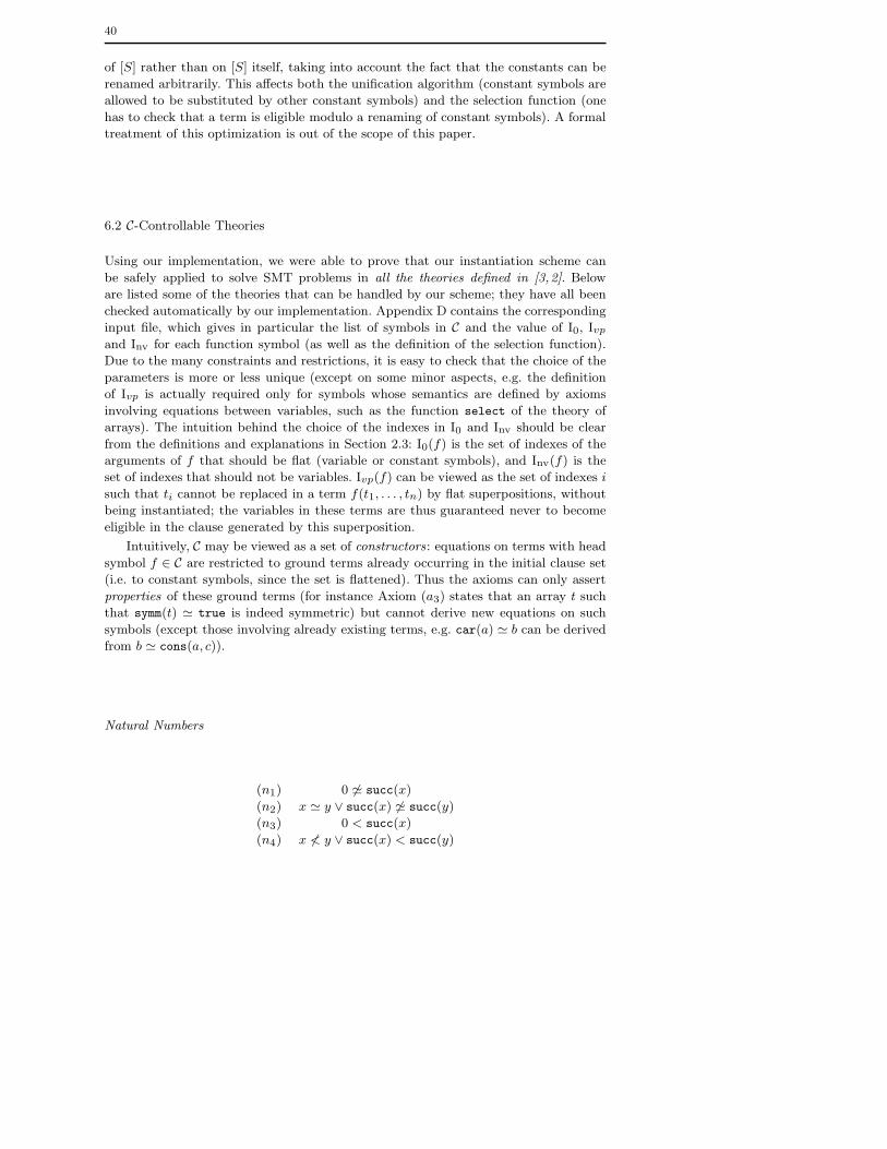
40

of [S] rather than on [S] itself, taking into account the fact that the constants can be

renamed arbitrarily. This affects both the unification algorithm (constant symbols are

allowed to be substituted by other constant symbols) and the selection function (one

has to check that a term is eligible modulo a renaming of constant symbols). A formal

treatment of this optimization is out of the scope of this paper.

6.2 C-Controllable Theories

Using our implementation, we were able to prove that our instantiation scheme can

be safely applied to solve SMT problems in all the theories defined in [3,2]. Below

are listed some of the theories that can be handled by our scheme; they have all been

checked automatically by our implementation. Appendix D contains the corresponding

input file, which gives in particular the list of symbols in C and the value of I0, Ivp

and Inv for each function symbol (as well as the definition of the selection function).

Due to the many constraints and restrictions, it is easy to check that the choice of the

parameters is more or less unique (except on some minor aspects, e.g. the definition

of Ivp is actually required only for symbols whose semantics are defined by axioms

involving equations between variables, such as the function select of the theory of

arrays). The intuition behind the choice of the indexes in I0 and Inv should be clear

from the definitions and explanations in Section 2.3: I0(f) is the set of indexes of the

arguments of f that should be flat (variable or constant symbols), and Inv(f) is the

set of indexes that should not be variables. Ivp(f) can be viewed as the set of indexes i

such that ti cannot be replaced in a term f(t1, . . . , tn) by flat superpositions, without

being instantiated; the variables in these terms are thus guaranteed never to become

eligible in the clause generated by this superposition.

Intuitively, C may be viewed as a set of constructors: equations on terms with head

symbol f ∈ C are restricted to ground terms already occurring in the initial clause set

(i.e. to constant symbols, since the set is flattened). Thus the axioms can only assert

properties of these ground terms (for instance Axiom (a3) states that an array t such

that symm(t) ≃ true is indeed symmetric) but cannot derive new equations on such

symbols (except those involving already existing terms, e.g. car(a) ≃ b can be derived

from b ≃ cons(a, c)).

Natural Numbers

(n1) 0 6≃ succ(x)

(n2) x ≃ y ∨ succ(x) 6≃ succ(y)

(n3) 0 < succ(x)

(n4) x 6< y ∨ succ(x) < succ(y)

41

Integer Offsets

(i1) p(s(x)) ≃ x

(i2) s(p(x)) ≃ x

(i3) sn−i(x) 6≃ pi(x) n > 0

The theory of Integer Offsets Modulo k can also be handled.

Ordering

(o1) x 6≺ y ∨ y 6≺ z ∨ x ≺ z

(o2) x 6≺ y ∨ y 6≺ x

Arrays

(a1) select(store(x, z, v), z) ≃ v

(a2) z ≃ w ∨ select(store(x, z, v), w) ≃ select(x,w)

(a3) symm(x) 6≃ true ∨ select(select(x, z), w) ≃ select(select(x,w), z)

(a4) injective(x) 6≃ true ∨ z ≃ w ∨ select(x, z) 6≃ select(x,w)

The theory of records can be handled in a similar way. The literals symm(t) 6≃ true

and injective(t) 6≃ true must be selected in the clauses above.

Encryption

(e1) dec(enc(x, y), y) = x

(e2) enc(dec(x, y), y) = x

These axioms encode encryption and decryption with a symmetric key. The encryp-

tion operation takes a clear-text and a key and produces a cipher-text. The decryption

operation inverses the encryption by extracting a clear-text from a cipher-text using

the same key.

(Possibly Empty) Lists

(l1) car(cons(x, y)) ≃ x

(l2) cdr(cons(x, y)) ≃ y

(l3) x ≃ nil ∨ cons(car(x),cdr(x)) ≃ x

(l4) cons(x, y) 6≃ nil

42

(Possibly Empty) Doubly Linked Lists

(ll1) x = nil ∨ next(x) = nil ∨ prev(next(x)) = x

(ll2) x = nil ∨ prev(x) = nil ∨ next(prev(x)) = x

(ll3) prev(x) ≃ nil ∨ prev(y) ≃ nil ∨ x ≃ y ∨ x ≃ nil ∨ y ≃ nil

∨prev(x) 6≃ prev(y)

(ll4) next(x) ≃ nil ∨ next(y) ≃ nil ∨ x ≃ y ∨ x ≃ nil ∨ y ≃ nil

next(x) 6≃ next(y)

ll3 and ll4 are logical consequence of ll1, ll2, but it is necessary to include these

axioms explicitly in order to satisfy the conditions of Definition 21.

Other recursive data-structures can be handled in a similar way.

Others

The union of these theories is also C-controllable. Furthermore, if a theory T is C-

controllable, and if S is a set of clauses containing only C-equations and ground flat

clauses, then T ∪S is also C-controllable (see Proposition 10). This property is essential

in practice, because one only has to check the controllability condition once and for all

on T .

One interesting point is that the superposition calculus does not necessarily ter-

minate on C-controllable clause sets. For instance, g(x) ≃ f(g(y)) is obviously C-

controllable (even controlled), but the superposition calculus deduces an infinite num-

ber of clauses of the form g(x) ≃ fn(g(y)). This shows evidence of the interest of the

instantiation method introduced in Section 3.

Sometimes non-controlled clauses may be reduced to controlled ones by simple

equivalence-preserving transformations. For instance, assume that the signature is

sorted and that an ordering ≺ on the sort symbols is given. Assume furthermore that

there exists a sort s such that for every function f : s1 × . . . × sn → s and for every

i ∈ [1..n]: si ≺ s. Then every quantified formula ∀x : s.φ can be replaced by the (equiv-

alent) conjunction:∧

f :s→s ∀x : s.φ{x → f(x)}. f ranges over the set of functions of

range s and x denotes a vector of distinct fresh variables of sort s. This process nec-

essarily terminates since a variable of sort s is replaced by variables of sorts strictly

lower than s.

If the previous property holds for every sort symbol (i.e. the clause set is stratified

in the sense of [1]), then the clause set can be transformed into an equivalent controlled

one by repeating this transformation for every non-minimal sort. It is easy to check

that the obtained formula is controlled (it suffices to take for every function symbol of

arity n, Inv(f) = [1..n] if the range of f is not minimal and I0(f) = [1..n] otherwise).

Another interesting case is when S contains terms of depth at most 1. S is nec-

essarily I0-flat and Inv-closed (it suffices to take I0(f) = [1..n] for every symbol f of

arity n). Then S is controlled if and only if it is variable-preserving. Thus the class of

variable-preserving clauses of depth 1 is decidable, although the superposition calculus

does not terminate on this class and the corresponding Herbrand universe is infinite in

the general case.

43

6.3 An Example of Application: the Theory of Arrays

It is worth investigating how our approach applies to well-known theories, such as the

theory of arrays, for which efficient instantiation schemes are already known (see for

instance [36,27,8,19]). Let φ be a ground formula built on a signature containing only

constant symbols and the functions select and store, as defined by Axioms (a1) and

(a2). By flattening and (structural) transformation into clausal normal form, φ can

be reduced to an equisatisfiable set of ground clauses S1 ∪ S2 where S2 is flat and S1

only contains equations of the form select(a, i) ≃ e and store(a, i, e) ≃ b (a, b, i, e are

constant symbols). As seen before, {(a1), (a2)} ∪S1 ∪S2 is C-controllable. The instan-

tiation scheme can be applied as follows. Obviously, the instantiation rule (I) applies

on the clauses (a1) and (a2), using the terms store(x, z, v) and store(a, i, e) and gen-

erates instances select(store(a, i, e), i) ≃ e and i ≃ w ∨ select(store(a, i, e), w) ≃

select(a,w), for every equation of the form store(a, i, e) ≃ b occurring in S2. This

step is rather standard and similar to what is done in existing approaches (see for

instance [12,7]). Then the rule may be applied to the term select(a,w), to gener-

ate the following ground clause: i ≃ i′ ∨ select(store(a, i, e), i′) ≃ select(a, i′), for

each previously generated clause and for each term of the form select(a′, i′) ≃ e′

occurring in S1. If the clauses are normalized during the instantiation step, replac-

ing the terms store(a, i, e) by b, then one could obtain instead: select(b, i) ≃ e and

i ≃ i′ ∨ select(b, i′) ≃ select(a, i′).

Note that variable w is only instantiated by the indices really occurring in a select

term. This is (probably) not very significant if the instantiation scheme is applied

eagerly (i.e. once and for all on the initial clause set), because in this case it is very

likely that every constant of sort index will appear as the second argument of a select

(besides pathological cases). However, if the instantiation scheme is applied lazily then

since the current branch does not contain in general all literals of head select, many

potential indexes may be discarded.

Obviously, the instantiation rule can also be applied the other way round. First

the term select(store(x, z, v), z) in (a1) can be pseudo-unified with select(a′, i′),

yielding a clause select(store(x, i′, v), i′) ≃ v, and then the rule can be applied to

the term store(x, i′, v), which produces: i ≃ i′ ∨ select(store(a, i′, e), i′) ≃ e. But

obviously the resulting clause is less general than select(store(a, i, e), i) ≃ e, thus it

is redundant.

To summarize, the non-ground axioms (a1) and (a2) can be replaced by the ground

set consisting of (a1) and (a2) instantiated by λ, along with select(store(a, i, e), i) ≃ e

and i ≃ i′∨select(store(a, i, e), i′) ≃ select(a, i′) (or, if clauses are normalized on the

fly, by select(b, i) ≃ e and i ≃ i′ ∨ select(b, i′) ≃ select(a, i′)), for every equations

store(a, i, e) ≃ b and select(b′, i′) ≃ e′ occurring in S1.

6.4 Experimental Results

We illustrate our approach by applying it on a standard example (see for instance [2]),

namely the commutativity of the store operation: the result of storing a set of elements

at distinct positions in an array does not depend on the ordering on the elements.

Formally, if γ is a permutation of [1..n], then {(a1), (a2),∧

0≤j<k≤n ij 6≃ ik} |= tn ≃ sn,

where tn and sn are defined inductively as follows:

44

– t0def

= s0def

= t,

– tk+1def

= store(tk, ik+1, uk+1),

– sk+1def

= store(sk, iγ(k+1), uγ(k+1)).

This is encoded by considering 4 lists of constant symbols: i1, . . . , in, j1, . . . , jn,

u1, . . . , un, v1, . . . , vn. Intuitively jk and vk denote iγ(k) and uγ(k) respectively. One

has to state that (jk, vk)k∈[1..n] is a permutation of (ik, vk)k∈[1..n] which is stated as

follows:∧n

l=1

∧nk=i+1(il 6≃ ik) ∧

∧nl=1

∨nk=1(il ≃ jk) ∧ (ul ≃ vk).

Since there are exponentially many possible distinct permutations, the difficulty of

the problem increases very quickly. For instance, for n = 2, we obtain the conjunction

of the following formulae:

(a1)

(a2)

store(store(t, i1, u1), i2, u2) ≃ store(store(t, j1, v1), j2, v2)

i1 6≃ i2

[(i1 ≃ j1) ∧ (u1 ≃ v1)] ∨ [(i1def

= j2) ∧ (u1 ≃ v2)]

[(i2 ≃ j1) ∧ (u2 ≃ v1)] ∨ [(i2def

= j2) ∧ (u2 ≃ v2)]

We provide the results (in seconds) obtained with our instantiation scheme com-

bined with the SMT-solver Yices [22] which is used to check the validity of the resulting

set of ground instances (in the empty theory) and with Yices alone, using built-in im-

plementation for the theory of arrays. Yices uses E-matching [20] and the method

described in [12] as heuristics for instantiating universally quantified variables. The

instantiation time is included, but it is very short (a few ms), even on the larger in-

stances.

n (I)+Yices Yices alone

5 0.078 0.063

7 0.391 0.344

8 1.234 1.094

9 7.781 6.828

10 38.375 98.563

11 1033.06 2018.5

As can be seen from the above table, our instantiation scheme (applied eagerly) is

fully competitive with Yices’s lazy instantiation technique. It is even more efficient on

harder instances. This may be due to the fact that when n is large enough, the number

of branches in the DPLL tree becomes so important that it is more efficient to perform

the instantiation once and for all at the root level.

Of course, our generic approach is more relevant and useful when applied on the-

ories (or combination of theories) for which no semantic instantiation scheme is avail-

able. Consider the following example. Obviously, a symmetric array stays so when the

following operations are performed:

– Replacement of the elements on the diagonal by arbitrary values.

– Replacement of the symmetrical elements at positions [i, j] and [j, i] by the same

value.

The formula below encodes these properties for a sequence of n operations. Starting

from an array t, we successively replace the element at position [ei, e′i] by vi and the

45

element at position [e′i, ei] by v′i, where for every i ∈ [1..n], either ei = e′i or vi = v′i.

More precisely, for every n ∈ N, we have

{(a1), (a2), (a3), symm(t), E} |= select(select(tn, z), w) ≃ select(select(tn, w), z),

where:

– Edef

=∧n

i=1 ei ≃ e′i ∨ vi ≃ v′i;

– tn is defined as follows:

– t0def

= t,

– t′idef

= store(ti, ei+1, store(select(ti, ei+1), e′i+1, vi+1)).

– ti+1def

= store(t′i, e′i, store(select(t

′i, e

′i), ei, v

′i)),

Bidimensional arrays are encoded as arrays whose elements are 1-dimensional ar-

rays. Of course, it would be possible (and actually much more natural and conve-

nient) to extend the axioms (a1), (a2) in order to handle pairs of indexes. We prefer

to use bidimensional arrays to make the problem artificially more difficult. Solving the

same problem with bidimensional arrays is actually a trivial task, since only one non-

redundant instance of Axiom (a3) may be generated (both our instantiation scheme

and Yices’s quantifier elimination heuristics detect this).

For instance, for n = 2, we obtain:

(a1)

(a2)

(a3)

symm(t)

e1 ≃ e′1 ∨ v1 ≃ v′1e2 ≃ e′2 ∨ v′2 ≃ v′2

t′0 = store(t, e′1, store(select(t, e1), e′1, v1))

t1 = store(t′0, e1, store(select(t, e′1), e1, v

′1))

t′1 = store(t1, e′2, store(select(t, e2), e

′2, v2))

t2 = store(t′1, e2, store(select(t, e′2), e2, v

′2))

select(select(t, i), j) 6≃ select(select(t, j), i)

The results are summarized in the following table. They show that our instanti-

ation scheme is less efficient than the one used by Yices on this example. However

completeness is not guaranteed for the latter. Other systems (such as CVC3 or Z3)

that fully implement the instantiation procedure described in [12] for extensions of the

theory of arrays are also complete on these benchmarks.

n (I)+Yices Yices alone

3 0.093 0.078

4 0.14 0.312

5 3.094 1.672

6 19.844 14.062

7 82.703 40.703

8 255.718 88.094

We now provide a simple example that is outside the scope of Yices’s quantifier

elimination heuristics. ¿From an n-dimensional array t, one can construct n arrays

of dimension n − 1: t′1, . . . , t′n by considering successively the projections of t on the

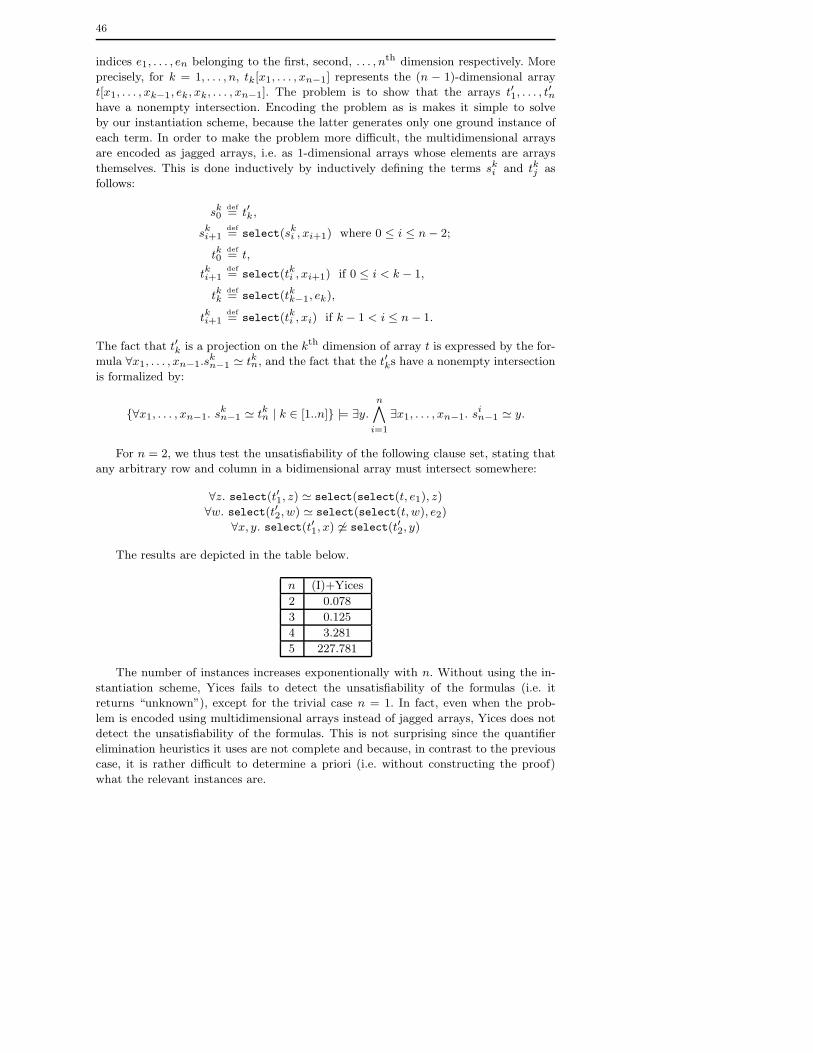
46

indices e1, . . . , en belonging to the first, second, . . . , nth dimension respectively. More

precisely, for k = 1, . . . , n, tk[x1, . . . , xn−1] represents the (n − 1)-dimensional array

t[x1, . . . , xk−1, ek, xk, . . . , xn−1]. The problem is to show that the arrays t′1, . . . , t′n

have a nonempty intersection. Encoding the problem as is makes it simple to solve

by our instantiation scheme, because the latter generates only one ground instance of

each term. In order to make the problem more difficult, the multidimensional arrays

are encoded as jagged arrays, i.e. as 1-dimensional arrays whose elements are arrays

themselves. This is done inductively by inductively defining the terms ski and tkj as

follows:

sk0def

= t′k,

ski+1def

= select(ski , xi+1) where 0 ≤ i ≤ n− 2;

tk0def

= t,

tki+1def

= select(tki , xi+1) if 0 ≤ i < k − 1,

tkkdef

= select(tkk−1, ek),

tki+1def

= select(tki , xi) if k − 1 < i ≤ n− 1.

The fact that t′k is a projection on the kth dimension of array t is expressed by the for-

mula ∀x1, . . . , xn−1.skn−1 ≃ tkn, and the fact that the t′ks have a nonempty intersection

is formalized by:

{∀x1, . . . , xn−1. skn−1 ≃ tkn | k ∈ [1..n]} |= ∃y.

n∧

i=1

∃x1, . . . , xn−1. sin−1 ≃ y.

For n = 2, we thus test the unsatisfiability of the following clause set, stating that

any arbitrary row and column in a bidimensional array must intersect somewhere:

∀z. select(t′1, z) ≃ select(select(t, e1), z)

∀w. select(t′2, w) ≃ select(select(t, w), e2)

∀x, y. select(t′1, x) 6≃ select(t′2, y)

The results are depicted in the table below.

n (I)+Yices

2 0.078

3 0.125

4 3.281

5 227.781

The number of instances increases exponentionally with n. Without using the in-

stantiation scheme, Yices fails to detect the unsatisfiability of the formulas (i.e. it

returns “unknown”), except for the trivial case n = 1. In fact, even when the prob-

lem is encoded using multidimensional arrays instead of jagged arrays, Yices does not

detect the unsatisfiability of the formulas. This is not surprising since the quantifier

elimination heuristics it uses are not complete and because, in contrast to the previous

case, it is rather difficult to determine a priori (i.e. without constructing the proof)

what the relevant instances are.

47

7 Discussion

In this paper we presented an instantiation scheme that permits to solve SMT problems

in several theories of interest by simply testing the satisfiability of a set of ground

clauses in first-order logic with equality. We also provided a set of syntactic conditions

that guarantee the completeness of the scheme; these conditions have been implemented

and were used to prove the scheme can be applied to the theories of Section 6. Note

that these conditions do not assume that the set of axioms is saturated, although some

partial saturation is sometimes required (see Section 5). The present paper is mostly

focused on theoretical issues although some preliminary experiments are presented.

The scheme itself can be integrated into any SMT solver. Such an integration would

permit to test which of the eager or lazy instantiation modes is the more efficient in

practice. It will also be interesting to see whether model generation techniques can be

applied to our setting, to generate relevant counter-examples for SMT problems.

There are some theories that are quite simple to define, but cannot be handled

by our scheme. One such example is the theory of arrays, augmented with a constant

predicate. This theory is defined by the axioms (a1), (a2) of Section 6, along with

axioms of the form

(cst) ¬cst(a, v) ∨ select(a, x) ≃ v.

The predicate cst(a, e) expresses the fact that the array a only contains the value e.

This theory cannot be controlled. Indeed, since the equation z ≃ w occurs in (a2), w

must occur in IV (select(store(x, z, v), w) ≃ select(x,w)), according to Definition

13. But in this case, index 2 must be in Ivp(select), and the clause select(a, x) ≃ v

cannot be variable-preserving, since x ∈ IV(select(a, x)) but x does not occur in the

term v. This theory is not C-controllable either, since this would imply that select ∈ C,

so that (a2) or (cst) can be reduced into a controlled clause by superposition from a

C-equation, (see Point 3 of Definition 21). But obviously, in this case new C-equations

can be derived (e.g. by superposition into the term store(x, z, v) of (a1)). These C-

equations are not strongly controlled by Definition, and this is explicitly forbidden by

Point 4 of Definition 21. It turns out that the instantiation scheme is not complete for

this theory. For example, the set of ground equations

1 : cst(a, 0),

2 : cst(b, 1),

3 : b ≃ store(a, 0, 1),

4 : 0 6≃ 1

is unsatisfiable. Indeed, clauses 1 and 2 imply that select(a, 1) ≃ 0, select(b, 1) ≃ 1.

But since b ≃ store(a, 0, 1) and 0 6≃ 1 we have by (a2): select(b, 1) ≃ select(a, 1) ≃0 6≃ 1. However, it is easy to check that the instantiation scheme cannot instantiate

the variable w in (a2) by 1, since 1 does not occur on the scope of a function symbol

select. Thus the clause set obtained by instantiation is satisfiable. A closer inspection

of this example shows that the theory of arrays augmented with a constant predicate

can entail a finite cardinality clause, and our scheme does not handle these clauses,

since they are trivially variable-eligible. We intend to investigate how such problematic

cases can be avoided by applying the instantiation scheme to only a limited number of

the clauses under consideration, in order to reason modulo the remaining clauses. This

might allow us to handle specific theories such as bitvectors, or infinitely axiomatized

theories, such as Presburger arithmetic or acyclic data structures.

48

Another direction to explore is how to raise the restriction that the instantiation

rule only takes into account ground terms that occur in the original set of clauses.

We intend to investigate how the heuristic techniques for quantifier reasoning may

permit to consider new complex terms that can be used by the instantiation rule.

Hopefully, taking these new terms into account will lead to a new scheme which will be

incomplete, as it may falsely assert that a set is satisfiable, but will be able to perform

more quantifier reasoning.

Another point that also deserves further investigation is the definition of an efficient

algorithm for computing, for a given a clause set S, all the necessary parameters that

make S controllable: selection function, ordering, set of function symbols C and index

functions I0, Inv and Ivp. Our current implementation assumes that all these parameters

are given, and we intend to implement several optimizations in an upcoming version

of our program. Actually, the difficult point is to compute the selection function (a

crucial point, as evidenced by Example 13) and the set of symbols C. Then the index

functions may be easily derived from the definitions.

Acknowledgements

We wish to thank the anonymous referees for their insightful comments which helped

improve an earlier version of this paper.

References

1. A. Abadi, A. Rabinovich, and M. Sagiv. Decidable fragments of many-sorted logic. Journalof Symbolic Computation, 45(2):153 – 172, 2010.

2. A. Armando, M. P. Bonacina, S. Ranise, and S. Schulz. New results on rewrite-based satis-fiability procedures. ACM Transactions on Computational Logic, 10(1):129–179, January2009.

3. A. Armando, S. Ranise, and M. Rusinowitch. A rewriting approach to satisfiability pro-cedures. Information and Computation, 183(2):140–164, 2003.

4. F. Baader and W. Snyder. Unification theory. In A. Robinson and A. Voronkov, editors,Handbook of Automated Reasoning, volume I, chapter 8, pages 445–532. Elsevier Science,2001.

5. L. Bachmair and H. Ganzinger. Rewrite-based equational theorem proving with selectionand simplification. Journal of Logic and Computation, 3(4):217–247, 1994.

6. C. Barrett, R. Sebastiani, S. Seshia, and C. Tinelli. Satisfiability modulo theories. InA. Biere, M. J. H. Heule, H. van Maaren, and T. Walsh, editors, Handbook of Satisfiability,volume 185 of Frontiers in Artificial Intelligence and Applications, chapter 26, pages 825–885. IOS Press, 2009.

7. C. W. Barrett, D. L. Dill, and A. Stump. Checking satisfiability of first-order formulasby incremental translation to sat. In E. Brinksma and K. G. Larsen, editors, CAV 2002,volume 2404 of LNCS, pages 236–249. Springer, 2002.

8. M. Bofill, R. Nieuwenhuis, A. Oliveras, E. Rodrıguez-Carbonell, and A. Rubio. A write-based solver for sat modulo the theory of arrays. In FMCAD ’08: Proceedings of the2008 International Conference on Formal Methods in Computer-Aided Design, pages 1–8, Piscataway, NJ, USA, 2008. IEEE Press.

9. M. P. Bonacina and M. Echenim. On variable-inactivity and polynomial T-satisfiabilityprocedures. Journal of Logic and Computation, 18(1):77–96, 2008.

10. M. P. Bonacina and M. Echenim. Theory decision by decomposition. Journal of SymbolicComputation, 45(2):229–260, 2010.

49

11. M. P. Bonacina, S. Ghilardi, E. Nicolini, S. Ranise, and D. Zucchelli. Decidability and un-decidability results for Nelson-Oppen and rewrite-based decision procedures. In U. Furbachand N. Shankar, editors, Proc. IJCAR-3, volume 4130 of LNAI, pages 513–527. Springer,2006.

12. A. R. Bradley and Z. Manna. The Calculus of Computation: Decision Procedures withApplications to Verification. Springer-Verlag New York, Inc., Secaucus, NJ, USA, 2007.

13. A. R. Bradley, Z. Manna, and H. B. Sipma. What’s decidable about arrays? In E. A.Emerson and K. S. Namjoshi, editors, Proc. VMCAI-7, volume 3855 of LNCS, pages427–442. Springer, 2006.

14. G. B. Dantzig and B. C. Eaves. Fourier-motzkin elimination and its dual. J. Comb.Theory, Ser. A, 14(3):288–297, 1973.

15. M. Davis, G. Logemann, and D. Loveland. A Machine Program for Theorem Proving.Communication of the ACM, 5:394–397, 1962.

16. M. Davis and H. Putnam. A Computing Procedure for Quantification Theory. Journal ofthe ACM, 7(3):201–215, July 1960.

17. L. de Moura and N. Bjørner. Engineering DPLL(T) + saturation. In A. Armando,P. Baumgartner, and G. Dowek, editors, IJCAR-4, volume 5195 of LNAI, pages 475–490.Springer, 2008.

18. L. M. de Moura and N. Bjørner. Efficient E-Matching for SMT Solvers. In F. Pfenning,editor, CADE-21, volume 4603 of LNCS, pages 183–198. Springer, 2007.

19. L. M. de Moura and N. Bjørner. Generalized, efficient array decision procedures. InFMCAD, pages 45–52. IEEE, 2009.

20. L. M. de Moura and N. Bjrner. Efficient e-matching for smt solvers. In F. Pfenning,editor, 21st International Conference on Automated Deduction, volume 4603 of LNCS,pages 183–198. Springer, 2007.

21. D. L. Detlefs, G. Nelson, and J. B. Saxe. Simplify: a theorem prover for program checking.Journal of the ACM, 52(3):365–473, 2005.

22. D. Dutertre and L. de Moura. The YICES SMT-solver, 2006. In SMT-COMP: SatisfiabilityModulo Theories Competition. Available at http://yices.csl.sri.com.

23. M. Echenim and N. Peltier. Instantiation of SMT problems modulo Integers. In AISC2010 (10th International Conference on Artificial Intelligence and Symbolic Computa-tion), LNCS. Springer, 2010.

24. H. Ganzinger and K. Korovin. Integrating equational reasoning into instantiation-basedtheorem proving. In Computer Science Logic (CSL’04), volume 3210 of LNCS, pages71–84. Springer, 2004.

25. Y. Ge, C. W. Barrett, and C. Tinelli. Solving quantified verification conditions usingsatisfiability modulo theories. Annals of Mathematics and Artificial Intelligence, 55(1-2):101–122, 2009.

26. Y. Ge and L. M. de Moura. Complete instantiation for quantified formulas in satisfiabilibymodulo theories. In A. Bouajjani and O. Maler, editors, CAV 2009, volume 5643 of LNCS,pages 306–320. Springer, 2009.

27. A. Goel, S. Krstic, and A. Fuchs. Deciding array formulas with frugal axiom instantiation.In SMT ’08/BPR ’08: Proceedings of the Joint Workshops of the 6th International Work-shop on Satisfiability Modulo Theories and 1st International Workshop on Bit-PreciseReasoning, pages 12–17, New York, NY, USA, 2008. ACM.

28. S. Jacobs. Incremental instance generation in local reasoning. In F. Baader, S. Ghi-lardi, M. Hermann, U. Sattler, and V. Sofronie-Stokkermans, editors, Notes 1st CEDARWorkshop, IJCAR 2008, pages 47–62, 2008.

29. J. Jouannaud and C. Kirchner. Solving equations in abstract algebras: a rule based surveyof unification. In J.-L. Lassez and G. Plotkin, editors, Essays in Honor of Alan Robinson,pages 91–99. The MIT-Press, 1991.

30. C. Kirchner, H. Kirchner, and M. Rusinowitch. Deduction with symbolic constraints.Revue Francaise d’Intelligence Artificielle, 4(3):9–52, 1990.

31. H. Kirchner, S. Ranise, C. Ringeissen, and D.-K. Tran. Automatic combinability ofrewriting-based satisfiability procedures. In M. Hermann and A. Voronkov, editors, Proc.LPAR-13, volume 4246 of LNCS, pages 542–556. Springer, 2006.

32. S. Lee and D. A. Plaisted. Eliminating duplication with the hyper-linking strategy. Journalof Automated Reasoning, 9:25–42, 1992.

33. C. Lynch and D.-K. Tran. Automatic decidability and combinability revisited. In F. Pfen-ning, editor, CADE-21, volume 4603 of LNAI, pages 328–344. Springer, 2007.

50

34. D. A. Plaisted and Y. Zhu. Ordered semantic hyperlinking. Journal of Automated Rea-soning, 25(3):167–217, October 2000.

35. S. Ranise and D. Deharbe. Applying light-weight theorem proving to debugging andverifying pointer programs. In Proc. of the 4th Workshop on First-Order Theorem Proving(FTP’03), volume 86 of Electronic Notes in Theoretical Computer Science, 2003.

36. A. Stump, C. W. Barrett, D. L. Dill, and J. Levitt. A decision procedure for an extensionaltheory of arrays. In LICS ’01: Proceedings of the 16th Annual IEEE Symposium on Logicin Computer Science, page 29, Washington, DC, USA, 2001. IEEE Computer Society.

37. U. Waldmann and V. Prevosto. SPASS+T. In G. Sutcliffe, R. Schmidt, and S. Schulz,editors, Proc. ESCoR Workshop, FLoc 2006, volume 192 of CEUR Workshop Proceedings,pages 18–33, 2006.

The following technical appendices contain additional definitions and detailed proofs ofimportant theorems used in the paper.

A Proof of Theorem 3

A.1 Derivation trees

Handling derivations in the usual sense is not really convenient for proving Theorem 3 becauseone has to apply complex transformations on derivations, involving for instance renamingsof variables and propagations of instantiations. In order to properly handle these issues, weintroduce the notion of derivation trees. These derivation trees allow us to keep track of thevariables involved in derivations in a simple way.

We first fix a special deduction relation:

Definition 23 We denote by →σ the relation →σ

sel,<, where < denotes the smallest mono-

tonic ordering such that t < s if either t is a proper subterm of s or if t ∈ Σ0 and s 6∈ Σ0 andsel denotes the selection function defined as follows:

– sel(C) = C if C is flat.– Otherwise, sel(C) is the set of literals in C that are either not flat or not ground4.

This relation corresponds to a (partially) unrestricted version of the calculus (in the sensethat the conditions on the inferences are as weak as possible), which is of course inefficient,but correct.

Definition 24 (Derivation tree) The class of derivation trees for a set of clauses S is thesmallest set of expressions of the form τ = [C,T , σ], such that:

– C is a clause, called the root of the tree and denoted by root(τ);– T is a (possibly empty) set of pairwise variable-disjoint derivation trees for S;– σ is a substitution;– if T 6= ∅ then root(T ) →σ C; otherwise, C is of the form Dσ, where D ∈ S and σ is a

renaming.

The notation root(T ) is defined in a standard way as follows:

root(T )def

= {root(τ) | τ ∈ T }.

A derivation tree [C,T , σ] is flat if σ is flat and every derivation tree τ ∈ T is flat. A refutationtree is a derivation tree of root �.

51

[f(x1) ≃ g(x1), ∅, {x 7→ x1}] [f(x2) ≃ a, ∅, {x 7→ x2}]

[g(x1) ≃ a, •, {x2 7→ x1}] [g(x4) 6≃ a, ∅, {y 7→ x4}]

[a 6≃ a, •, {x1 7→ x4}]

[�,•, id]

{x2 → x1}

{x1 → x4}

id

Fig. 5 Derivation tree of Example 15

The set of clauses S may remain implicit, in which case we will simply talk about derivationtrees.

Example 15 Let S = {f(x) ≃ g(x), f(x) ≃ a, g(y) 6≃ a}. Then starting with the derivationtrees

τ1 = [f(x1) ≃ g(x1), ∅, {x 7→ x1}] and τ2 = [f(x2) ≃ a, ∅, {x 7→ x2}],

we may construct the derivation tree τ3 = [g(x1) ≃ a, {τ1, τ2}, σ], where σ = {x2 → x1}.Consider τ4 = [g(x4) 6≃ a, ∅, {y 7→ x4}] and σ′ = {x1 → x4}, then τ = [a 6≃ a, {τ3, τ4}, σ′]

and τ ′ = [�, {τ}, id] are derivation trees for S, which is unsatisfiable.A graphical representation of τ ′ is provided in Figure 5. The black dots denote the deriva-

tion trees immediately below.

When clear from the context, we will keep the substitutions implicit in the graphicalrepresentations.

A.2 Restricted classes of derivation trees

We now restate the conditions on the derivations using the more precise formalism of deriva-tion trees. The definition is actually slightly weaker than Definition 9 since the ordering andselection function are less restrictive.

Definition 25 (Simple Derivation Tree) Let S be a set of clauses. A derivation treeτ = [C,T , σ] of S, where σ is an mgu of two terms t, s, is simple if it satisfies the followingconditions:

1. σ is flat.2. C is I0-flat (see Section 2.3), and not variable-eligible (see Section 2.2).3. If there is a position p such that t|p = f(t1, . . . , tn) (resp. s|p = f(t1, . . . , tn)) and ti ∈ V

for some i ∈ Inv(f), then either s|p (resp. t|p) occurs in S or σ = id.

4 Obviously sel(C) contains all the maximal literals in C.

52

4. If C is obtained using superposition/paramodulation by replacing a term uσ by vσ, thenvσ 6∈ V .

5. Every derivation tree in T is simple.

A set of clauses S is simply provable if for all clauses C, if S admits a derivation tree ofroot C then S also admits a simple derivation tree of root C. A class of clause sets S is simplyprovable if every set of clauses in S is simply provable.

We first need to introduce additional definitions and results about derivation trees.

Definition 26 The depth of a derivation tree is inductively defined as follows:

depth([C, ∅, σ])def

= 0, and depth([C, T , σ])def

= 1 + maxτ∈T

depth(τ).

The set of variables occurring in a derivation tree τ , denoted by V(τ), is the set of variablesdefined as follows:

V([C, T , σ])def

= V(C) ∪⋃

τ ′∈T

V(τ ′)

where V(C) denotes the set of variables in C.

Example 16 In Example 15, the derivation tree τ ′ is of depth 3, and the set of variablesoccuring in τ ′ is V(τ ′) = {x1, x2, x4}.

We also define the composition of the unifiers over a derivation tree.

Definition 27 Given a derivation tree τ , the substitution µτ denotes the composition of theunifiers in τ , which is formally defined as follows:

µ[C,∅,σ]def

= id,

µ[C,T ,σ]def

= (⋃

τ∈T

µτ )σ.

This notation is well-defined since the trees in T are mutually variable-disjoint. Note thatthe initial renamings of clauses are not taken into account in the construction of µτ . Thus,these substitutions only make sense when applied to the clauses of S that have already beenrenamed.

Example 17 In Example 15, we have σ = {x2 → x1} and σ′ = {x1 → x4}, hence µτ = σσ′ ={x2 → x4, x1 → x4}, and µτ ′ = µτ .

We obtain a first result for keeping track of a variable in a derivation tree.

Proposition 16 Let τ = [C,T , σ] be a derivation tree. If x ∈ V(C) then x 6∈ dom(µτ ).

Proof By an immediate induction on the depth of the tree. The variable x cannot occur indom(σ), since by definition of the calculus, σ is applied to the clauses in T to generated C,and is idempotent.

We define a subclass of simple derivation trees that will serve as a link between a derivationtree for S and one for Sλ.

Definition 28 (Pure Derivation Trees) A derivation tree τ is pure if it is simple and ifµτ is pure (this implies that every subtree of τ is pure).

53

We define the notions of instantiated and uninstantiated hypotheses in a derivation tree.These sets represent the clauses occurring in the original set of clauses, in their instantiatedand uninstantiated versions.

Definition 29 Given a derivation tree τ , we denote by hyp(τ) the set of uninstantiated hy-potheses of τ , and by hypinst(τ) the set of instantiated hypotheses of τ . Formally:

hyp([C, ∅, σ])def

= hypinst([C, ∅, σ])def

= {Cσ},

hyp([C,T , σ])def

=⋃

τ∈T

hyp(τ),

hypinst([C,T , σ])def

=⋃

τ∈T

hypinst(τ)σ.

A clause C is a main hypothesis of a flat tree τ if C ∈ hyp(τ) and if for any variable x ∈ V(C)and for any unifier σ occuring in τ , we have xσ ∈ V(C) ∪Σ0.

Example 18 Suppose τ = [�,T , {x → a}], where T = {[p(x, b), ∅, id], [¬p(a, y), ∅, id]}. Thenhyp(τ) = {p(x, b),¬p(a, y)} and hypinst(τ) = {p(a, b),¬p(a, b)}.

It will sometimes be useful to replace a subtree in a simple or pure derivation tree byanother one. This operation is harmless. Consider for example a derivation tree τ = [C,T , σ]that is simple (resp. pure), and let τ ′ ∈ T . Let τ ′′ be a simple (resp. pure) derivation treewith the same root as τ ′, and such that the only variables τ and τ ′′ have in common are thoseoccurring in root(τ ′′). Then [C,T ′, σ], where T ′ = (T \ {τ ′}) ∪ {τ ′′}, is a simple (resp. pure)derivation tree with the same root as τ . This result can be generalized to any subtree of τ :

Proposition 17 Let τ be a simple (resp. pure) derivation tree for a set of clauses S, andτ ′ = [C,T , σ] be a subtree of τ . Let τ ′′ be a simple (resp. pure) derivation tree for S suchthat:

– τ ′ and τ ′′ have the same root,– the only variables τ and τ ′′ have in common are those occurring in C.

Then the derivation tree obtained by replacing τ ′ by τ ′′ in τ is also a simple (resp. pure)derivation tree for S, with the same root as τ .

If τ and τ ′′ have more variables in common than those in C, then the other variablescan of course be renamed, thus yielding a derivation tree that satisfies all the conditions ofProposition 17.

Example 19 Consider the set of clauses

S = {f(x) ≃ f ′(x), f(x) ≃ g′(x), f ′(x) ≃ h(x), h(x) ≃ g′(x), g(x) ≃ h(x)}.

The derivation trees τ (top) and τ ′ (bottom) of Figure 6 have the same root and are bothpure; τ ′ was obtained from τ by replacing the subtree of root f(x2) ≃ h(x2), with the dashedlines, by the subtree with the bold lines. Note that these subtrees only have x2 as a commonvariable.

We define a last class of derivation trees, the most constrained one, which permits onlybasic inferences to be carried out on a set of clauses. This class will allow us to discard thebasic inferences in the construction of a derivation tree.

Definition 30 (Elementary Derivation Tree) A derivation tree [C,T , σ] is elementary ifT = ∅ or T = {τ, τ ′}, where τ is elementary and τ ′ is pure and has a ground root.

Note that every elementary tree is pure. We introduce the following measure on derivationtrees:

54

[f(x4) ≃ f ′(x4), ∅] [f ′(x2) ≃ h(x2), ∅]

[f(x2) ≃ h(x2), •] [g(x3) ≃ h(x3), ∅]

[f(x3) ≃ g(x3), •]

[f(x2) ≃ g′(x2), ∅] [h(y1) ≃ g′(y1), ∅]

[f(x2) ≃ h(x2), •] [g(x3) ≃ h(x3), ∅]

[f(x3) ≃ g(x3), •]τ

τ ′

Fig. 6 Derivation trees of Example 19 (the substitutions are omitted for the sake of readabil-ity)

Definition 31 Given a derivation tree τ , the measure δ(τ) is defined inductively by:

– δ(τ)def

= 0 if τ is elementary.

– δ([C, T , σ])def

= 1 + maxτ∈T δ(τ) otherwise.

In particular, this measure is unaffected by the adjunction of a flat ground clause to ahypothesis in a pure derivation trees:

Proposition 18 Let τ = [C,T , σ] be a pure derivation tree for a set of clauses S, D ∈ hyp(τ),and consider a flat, ground clause E. Then there exists a pure derivation tree τ ′ of root C∨Efor S ∪ {D ∨E}, such that δ(τ ′) = δ(τ).

Proof We prove the result by induction on the depth of τ . If T = ∅, then the result is obvious,since necessarily C = D. Now assume T = {τ1, τ2}, where D1,D2 are the respective rootsof τ1, τ2, and w.l.o.g., suppose D ∈ hyp(τ1). Then by definition {D1, D2} →σ C, and by theinduction hypothesis, there is a pure derivation tree τ ′1 of root D1 ∨E for S ∪ {D ∨E}. Sinceno ordering conditions are considered in the calculus, the literals in E have no influence onthe derivation, and it is clear that {D1 ∨ E,D2} →σ C ∨ E. Thus, τ ′ = [C ∨ E, {τ ′1, τ2}, σ] isa pure derivation tree for S ∪ {D ∨ E}, and obviously, δ(τ ′) = δ(τ).

A.3 Swapping variables in pure derivation trees.

Given a pure derivation tree, we will sometimes construct a new derivation tree with the sameproperties as the original one, by swapping some of its variables, as in the following example.

55

Example 20 Let S = {f(x, y) ≃ g(x, y), f(y, y) ≃ h(y)}, and consider the clauses

C1 = f(x1, x2) ≃ g(x1, x2),C2 = f(y1, y1) ≃ h(y1),C = g(y1, y1) ≃ h(y1),

and the substitutions

σ1 = {x 7→ x1, y 7→ x2},

σ2 = {y 7→ y1}.

Let τ1 = [C1, ∅, σ1], τ2 = [C2, ∅, σ2], and σ = {x1 → y1, x2 → y1}; then τ = [C, {τ1, τ2}, σ] isa pure derivation tree for S.

Another pure derivation tree for S with root C can also be constructed by swapping x1

and y1. This tree is obtained by taking the clauses

C′1 = f(y1, x2) ≃ g(y1, x2),

C′2 = f(x1, x1) ≃ h(x1),

the substitutions

σ′1 = {x 7→ y1, y 7→ x2},

σ′2 = {y 7→ x1},

and the derivation trees τ ′1 = [C′1, ∅, σ

′1] and τ ′2 = [C′

2, ∅, σ′2]. Then τ ′ = [C, {τ ′1, τ

′2}, σ] is also

a pure derivation tree for S, and has the same root as τ .

To formalize the intuition of this example, we define the renaming of a derivation tree.

Definition 32 If τ = [C,T , σ] is a derivation tree and π is a renaming, then τπ denotes the

derivation tree defined as follows: τπdef

= [Cπ,T π, π−1σπ].

The next lemma shows that τπ is indeed a derivation tree with the same properties as τ .We prove the result in the case where τ is a pure derivation tree, along with some additionalproperties on its structure.

Lemma 14 Let τ = [C,T , σ] be a pure derivation tree for S and π be a renaming. Then τπis a pure derivation tree τ ′ for S such that root(τ ′) = Cπ, µτ ′ = π−1µτπ, hyp(τ ′) = hyp(τ)πand δ(τ ′) = δ(τ).

Proof The result is proven by induction on the depth of τ . If τ = [C, ∅, σ], then the resultis obvious. Now assume τ = [C,T , σ]. Let T = {τ1, τ2} (we may have τ1 = τ2) and let

τ ′idef

= τiπ (i = 1, 2). By the induction hypothesis, τ ′1 and τ ′2 are derivation trees, and we have

root(τi) = Ciπ, µτ ′

i

= π−1µτiπ, hyp(τ ′i ) = hyp(τi), δ(τ ′i ) = δ(τi) (for i = 1, 2). Then by

definition, σ is the mgu of two terms s and t, so that σ′ = π−1σπ is an mgu of sπ and tπ.

Thus, if T ′ = {τ ′1, τ′2}, then τ ′

def

= [Cπ,T ′, σ′] is a pure derivation tree for S (since π is arenaming, τ ′1 and τ ′2 do not share any variables). Furthermore, by definition,

µτ ′ = (⋃

τ ′

i∈T ′

µτ ′

i

)σ′

= (⋃

τ ′

i∈T ′

µτ ′

i

)σ′

= (⋃

τi∈T

π−1µτiπ)σ′ (by the induction hypothesis)

= π−1(⋃

τi∈T

µτi)πσ′

= π−1(⋃

τi∈T

µτi)σπ (because σ′ = π−1σπ)

= π−1µτπ

56

It is simple to verify that δ(τ ′) = δ(τ).

The previous lemma shows how pure derivation trees are preserved by renamings. In thesequel, we will sometimes need to rename variables in a pure derivation tree, without modifyingthe root of this derivation tree. The following lemma provides a sufficient condition for safelyperforming such an operation.

Lemma 15 Let τ = [C,T , σ] be a pure derivation tree for a set of clauses S, let x ∈ dom(σ)and consider π = {x→ xσ, xσ → x}. Then τ ′ = [C,T π, π−1σ] is a pure derivation tree for Ssuch that root(τ ′) = C, µτ ′ = π−1µτ , hyp(τ ′) = hyp(τ)π and δ(τ ′) = δ(τ).

Proof The proof is immediate if T = ∅. By Lemma 14, τ ′′ = [Cπ,T π, π−1σπ] is a purederivation tree for S of root Cπ, such that hyp(τ ′′) = hyp(τ)π, µτ ′′ = π−1µτπ, δ(τ ′′) = δ(τ),where π−1σπ is an mgu of two terms sπ and tπ. But since π is a renaming, (π−1σπ)π−1 =π−1σ is also an mgu of sπ and tπ, and the clause generated with this mgu is (Cπ)π−1 = C.Thus τ ′ = [C,T π, π−1σ] is a pure derivation tree for S. We have µτ ′ = µτ ′′π−1 = π−1µτ .

In Example 20, C1 and C2 are hypotheses of τ , but none of them is a main hypothesis.But by swapping variables x1 and y1, the new derivation tree we obtain is such that C′

1 is amain hypothesis for this tree. We show that it is possible to generalize this example.

Lemma 16 Let τ be a pure derivation tree for a set of clauses S, let D ∈ hyp(τ) and let udenote a term appearing in D. If θ is a ground substitution such that dom(θ) ⊆ V(u), thenthere exists a pure derivation tree τ ′ for S with the same root as τ , a substitution η, a clauseD′ = Dη ∈ hyp(τ ′) and a term u′ occurring in D′ such that:

– D′µτ ′ = Dµτ and u′µτ ′ = uµτ ,– D′ a main hypothesis,– the substitution θ′ = η−1θη corresponding to θ is such that dom(θ′)µτ ′ ⊆ dom(θ′).

Proof Assume that τ,D, u, θ do not satisfy the property above. In particular, ηdef

= id, D′ def

= D

and u′def

= u cannot be a solution, thus there must exist a variable x such that one of thefollowing conditions holds:

– either x ∈ V(D) and xµτ 6∈ V(D) (i.e. D is not a main hypothesis of τ),– or x ∈ dom(θ) and xµτ 6∈ dom(θ).

We denote by E(τ,D, u, θ) the set of variables x satisfying one of these properties. Bydefinition, for every x ∈ E(τ,D, u, θ), we have x ∈ dom(µτ ), thus there exists a (unique)subtree τx = [C,T , σ] of τ such that x ∈ dom(σ). Let m(τ,D, u, θ) denote the multiset definedby:

m(τ,D, u, θ)def

= {δ(τ) − δ(τx) | x ∈ E(τ,D, u, θ)}.

This measure m(τ,D, u, θ) is clearly well-founded, thus we may assume w.l.o.g. that the tuple(τ,D, u, θ) is the minimal one (according to m) such that the above property does not hold.

Let x ∈ E(τ,D, u, θ). Let τx = [C,T , σ] and x′ = xσ. We can safely replace τx by thepure derivation tree obtained as in Lemma 15. Let τ ′ be the pure derivation tree obtained by

replacing τx with this new derivation tree in τ . Let π = {x 7→ x′, x′ 7→ x} and θ′def

= π−1θπ.

By Lemma 15, hyp(τ ′) contains the clause D′ def

= Dπ and the term u′def

= uπ. We have D′µτ ′ =Dπµτ ′ . By Lemma 15, µτ ′ = π−1µτ thus D′µτ ′ = Dµτ and uµτ = u′µτ ′ .

By definition, we have x 6∈ E(τ ′,D′, u′, θ′), since x does not occur in D′. Let y be avariable distinct from x′, occurring in E(τ ′, D′, u′, θ′). We show that y ∈ E(τ,D, u, θ). Sinceτ ′ is obtained from τ by swapping x and x′ in some part of the tree and since xσ = x′σ = x′, wehave yµτ ′ = yµτ . We assume that y 6∈ E(τ,D, u, θ) to derive a contradiction. We distinguishtwo possibilities:

– If y ∈ V(D′) and yµτ ′ 6∈ V(D′), then since y 6= x, x′ we have y ∈ V(D) and sinceyµτ ′ = yµτ , yµτ 6∈ V(D′). If yµτ ∈ V(D) this would imply that yµτ = x, which isimpossible since xσ = x′.

57

– If y ∈ dom(θ′) and yµτ ′ 6∈ dom(θ′), then we have y ∈ dom(θ) (since y 6= x, x′) andyµτ 6∈ dom(θ′). If yµτ ∈ dom(θ), then necessarily yµτ = x′, thus x′ 6∈ dom(θ′), andx 6∈ dom(θ). This means that both x and x′ occur in D (x occurs in D since it is inE(τ,D, u, θ) by definition and x′ ∈ dom(θ) ⊆ V(D)). Moreover since yµτ = x′ we havex′µτ = x′ and xµτ = x′. Consequently, x and xµτ both occur in D and xµτ ∈ dom(θ).This contradicts the fact that x ∈ E(τ,D, u, θ).

Consequently, the only variable that may occur in E(τ ′, D′, u′, θ′) but not in E(τ,D, u, θ) isx′. If x′ ∈ E(τ ′, D′, u′, θ′) then δ(τ ′

x′) > δ(τx). Thus m(τ ′,D′, u′, θ′) < m(τ, D, u, θ). Since

τ is minimal, there exists a tree τ ′′ a clause D′′ and a term u′′ in D′′ satisfying the desiredproperties for τ ′,D′, u′. By transitivity, this also holds for τ,D, u.

Given a simple derivation tree τ of root C and a substitution θ, we provide a character-ization based on the main hypotheses of τ that guarantees the existence of another simplederivation tree whose root is Cθ. We first prove a unification property that will be used toguarantee the existence of this simple derivation tree.

Lemma 17 Let t, s be two unifiable terms and let σ = mgu(t, s) be a flat substitution. Let θ bea flat and ground substitution such that ∀x ∈ dom(θ), xθ = xσθ. Then tθ and sθ are unifiable.Furthermore, if η = mgu(tθ, sθ), then dom(η) = dom(σ) \ dom(θ) and for all x ∈ dom(η),xη = xσθ.

Proof A unification problem is a conjunction of equations (or false). If φ, ψ are two unificationproblems, then we write φ →unif ψ if ψ is obtained from φ by applying the usual replacement

or decomposition rules [29].σ is of the form {xi 7→ ui | i ∈ [1..m]}, where x1, . . . , xm are pairwise distinct variables not

occurring in u1, . . . , um. Moreover, there exists a sequence of unification problems (φi)i∈[1..n]

such that φ1 = (t =? s), ∀i ∈ [1..n− 1], φi →unif φi+1 and φn =∧m

i=1(xi =? ui). We assume

that the unification rules are applied with the following priority: decomposition first, thenreplacement by terms w such that wθ ∈ T0 and finally the remaining replacements.

Let k be an index in [1..n]. We shall prove that φkθ →∗unif

φk+1θ.

If φk+1 is obtained from φk by decomposition, then φk, φk+1 are respectively of the formf(t) =? f(s) ∧ ψ and t =? s ∧ ψ. Then φkθ is of the form f(t)θ =? f(s)θ ∧ ψθ, thus thedecomposition rule applies and deduces tθ =? sθ ∧ ψθ i.e. φk+1θ.

If φk+1 is obtained from φk by replacement then φk, φk+1 are respectively of the formx =? w ∧ ψ and x =? w ∧ ψ{x → w} where x is a variable in x1, . . . , xm and w is a term notcontaining x. By definition, x ∈ dom(σ). φkθ is xθ =? wθ ∧ ψθ.

If x 6∈ dom(θ) then xθ = x. x 6∈ V(wθ) (since x 6∈ V(w) and θ is ground). Thus thereplacement rule applies and deduces x =? wθ ∧ ψθ{x → wθ} i.e. φk+1θ.

Now assume that x ∈ dom(θ). We have, by definition, xσ = wσ, thus xσθ = wσθ and bythe above condition, since x ∈ dom(θ), xθ = wσθ. If w ∈ dom(θ), or if w 6∈ V then we havewσθ = wθ, thus xθ = wθ and φkθ = φk+1θ. If w ∈ V \ dom(θ) then we must have xσ 6= w(otherwise we would have wθ = xθ hence w ∈ dom(θ)). This means that w ∈ dom(σ) and wis replaced at some step. Thus there exists in the unification problem an equation of the formy =? xσ, where y ∈ V . But then, according to the above strategy, the replacement rule shouldhave been applied first on this equation before x =? w (since xσθ ∈ T0).

Therefore, we have tθ =? sθ →∗unif

∧mi=1(xiθ =? uiθ). By the above reasoning, for every

i, j ∈ [1..m], we have either xiθ = xi and xi 6∈ V(ujθ), or xi ∈ dom(θ) and xiθ = uiθ. Thus{xi 7→ uiθ | i ∈ [1..m], xi 6∈ dom(θ)} = mgu(tθ, sθ).

Lemma 18 Let S be a set of clauses and τ = [C,T , σ] be a simple derivation tree for S ofroot C. Consider a clause D that is a main hypothesis of τ and a flat and ground substitutionθ such that dom(θ) ⊆ V(D) and for all variables x ∈ dom(θ), xθ = xµτ θ. Assume furtherthat there exists a variable x0 ∈ V(D) such that x0µτ ∈ V(C). Then there exists a simplederivation tree τ ′ for S ∪ {Dθ}, of root Cθ, such that δ(τ ′) ≤ δ(τ).

58

Proof Let S′ = S ∪ {Dθ}, we will prove the result by induction on the depth of τ .

If T = ∅, necessarily, C = D, and Cθ ∈ S′. Thus τ ′def

= [Cθ, ∅, id] satisfies the requirements.Now assume that T = {τ1, τ2}, where root(τ1) = C1 = (t1 ≃ v) ∨ C′

1 and root(τ2) = C2[t2]p,and suppose that C is generated by superposition or paramodulation from C1 into C2, i.e.,σ = mgu(t1, t2) and C = (C′

1 ∨ C2[v]p)σ. By definition, there exists an i ∈ {1, 2} such thatD ∈ hyp(τi). Moreover, x0µτi

must occur in the root of τi, since x0µτ = x0µτiσ ∈ V(C) by

hypothesis, and V(C) ⊆ V(C1σ) ⊎ V(C2σ).Let θ′ be the restriction of σθ to the variables in D; note that θ and θ′ coincide on all

the variables not occurring in dom(σ). We check that we can apply the induction hypothesison the derivation tree τi and the substitution θ′. First, it is clear that D is a main hypothesisof τi, since τi is a subtree of τ . Now let x be a variable occurring in dom(θ′), we show thatxθ′ = xµτi

θ′. If xµτi= x, then the proof is obvious. If xµτi

is a constant, then x cannot belongto dom(σ) and of course, xµτi

θ′ = xµτi. Since x ∈ dom(θ′) ⊆ dom(σ) ∪ dom(θ), necessarily

x ∈ dom(θ), and by hypothesis, xθ = xµτ θ. This entails that

xθ′ = xσθ = xθ = xµτ θ = xµτiσθ = xµτi

.

Now assume xµτiis a variable other than x, and let y = xµτi

6= x. Note that y ∈ V(D) sinceD is a main hypothesis of τi. Since y 6= x, necessarily, x 6∈ dom(σ) (by Proposition 16, becausex ∈ dom(µτi

)). Furthermore, by definition, xµτ = yσ, thus:

xθ′ = xσθ = xθ = xµτ θ = yσθ = yθ′ = xµτiθ′.

Therefore, we may apply the induction hypothesis on τi and θ′: there exists a simple derivationtree τ ′i for S′, of root Ciθ

′, where δ(τ ′i ) ≤ δ(τi).Let j = 3−i, and let τ ′j = τjη be a renaming of τj that contains no variable occurring in τi

or τ ′i . Then of course, C′j = Cjη is the root of τ ′j . Since σ is a unifier of t1, t2 which are variable-

disjoint, the substitution σ′ such that ∀x ∈ V(Ci), xσ′def

= xσ and ∀x ∈ V(C′j), xσ

′ def

= xη−1σ

is well-defined, flat, and is an mgu of ti, tjη. We now prove that tiθ and tjηθ are unifiableby verifying that the application conditions of Lemma 17 are satisfied for ti, tjη and θ. Byhypothesis, θ is flat and ground, and ∀x ∈ dom(θ), xθ = xµτ θ. Furthermore, for all x ∈ V(ti),we have xµτ = xσ, and since σ and σ′ are identical on V(ti), xµτ = xσ′. Thus, for allx ∈ dom(θ), xθ = xσ′θ. Consequently, we can apply Lemma 17: tiθ and tjηθ are unifiable, andhave an m.g.u. γ such that dom(γ) = dom(σ′) \ dom(θ) and xγ = xσ′θ for all x ∈ dom(γ).

Since dom(θ) ⊆ V(D) and D is a main hypothesis, for all x ∈ V(ti) ∩ dom(θ), xσ ∈ V(D)and xσθ = xθ′. Hence,

tjηθ = tjη, and

tiθ = tiσθ = tiθ′.

Therefore, γ is a flat, ground mgu of tiθ′ and tjη, and the paramodulation rule is applicable

on the clauses Ciθ′ and Cjη.

We now prove that the generated clause is Cθ. To this aim, it suffices to show that Ciθ′γ =Ciσθ and Cjηγ = Cjσθ, since we use the unordered version of the calculus the inference stepare stable by instantiation.

Let x ∈ V(Ci). If x ∈ V(D) then xθ′ = xσθ. By definition of γ, this implies that xθ′γ =xσθ. If x 6∈ V(D), then xθ′ = xθ = x, hence xθ′γ = xγ = xσ′θ′. By definition of σ′, we havexσ′ = xσ. Furthemore, xσθ′ = xσθ.

Now, let x ∈ V(Cj ). By definition x 6∈ dom(θ), hence xθ = x. If xη 6∈ dom(σ′), thenxηγ = x. Moreover, this implies that x 6∈ dom(σ) thus xσθ = xθ = x, and the proof iscompleted. Otherwise, by definition of γ, xηγ = xσθ.

Thus {Ciθ′, Cjη} →γ Cθ and the derivation tree τ ′ = [Cθ, {τ ′1, τ

′2}, γ] satisfies the desired

result. This derivation tree is simple since it is obtained by instantiating simple derivation treesby a flat substitution (it is easy to verify that all the conditions in Definition 25 are satisfied).

If τ is nonelementary then δ(τ) = 1 + max(δ(τ1), δ(τ2)) ≥ 1 + max(δ(τ ′1), δ(τ ′2)) = δ(τ ′).Otherwise, since the root of τi cannot be ground (since it contains the variable x0µτi

), τimust be elementary. Since δ(τ ′i ) ≤ δ(τi), necessarily, τ ′i is elementary. Furthermore, τj mustbe pure and have a ground root, hence, τ ′j is also pure and has a ground root. Therefore, τ ′ is

elementary and δ(τ) = δ(τ ′) = 0.The proof is similar if C is deduced using a unary inference step (reflection or equational

factorisation).

59

A.4 Some properties of the relations ≡SC

We state some properties of the relation ≡SC

of Definition 2.

Definition 33 A set of clauses S is Σ0-stable if for every pair of clauses (C[a]p, a ≃ b ∨ D)occurring in S, the clause C[b]p ∨D also occurs in S.

Lemma 19 Let S be a set of clauses and C be a flat ground clause. If S is Σ0-stable then≡S

C is an equivalence relation.

Proof ≡SC is reflexive by definition. Moreover it is symmetric by the commutativity of ≃. We

only have to show that it is transitive. Assume that a ≡SD c and c ≡S

D b, for some terms

a, b, c. We show that a ≡SDb. The proof is by induction on the depth of the terms. If a = c

or c = b the proof is trivial. If a = f(a1, . . . , an) is complex, then by definition c must be ofthe form f(c1, . . . , cn) where ∀i ∈ [1..n].ai ≡S

D ci. Similarly, we have b = f(b1, . . . , bn) and

∀i ∈ [1..n].ci ≡SDbi. By the induction hypothesis, we have ∀i ∈ [1..n].ai ≡S

Dbi hence a ≡S

Db.

If a is flat, then we must have a, b, c ∈ Σ0 and S contains two clauses (a ≃ c) ∨ D1 and(c ≃ b) ∨D2 where D1,D2 ⊆ D. By ground superposition (since the constant are unordered)we can derive (a ≃ b)∨D1 ∨D2 from (a ≃ c)∨D1 and (c ≃ b)∨D2. Since S is Σ0-stable, thisclause must occur in S. Therefore, a ≡S

Cb.

The relation �SC

below provides a link between any complex term occurring in the root ofa pure derivation tree, and the complex terms occurring in the original set of clauses.

Definition 34 Let S denote a set of clauses and C be a flat, ground clause.Given two terms t = f(t1, . . . , tn) and s = f(s1, . . . , sn), we write t �S

Cs if for all i ∈ [1..n],

if ti ∈ T0 or si ∈ V , then ti ≡SC si.

We prove some simple results on the relation �SC

: this relation is stable by instantiationand inclusion, and it is transitive.

Proposition 19 Let C be a flat ground clause and S be a Σ0-stable set of clauses. Then �SC

is transitive.

Proof Assume that t �SC s �S

C u. By definition of �SC we have t = f(t1, . . . , tn), s =

f(s1, . . . , sn), u = f(u1, . . . , un). Let i ∈ [1..n]. If ti ≡SCsi and si ≡S

Cui then ti ≡S

Cui

by transitivity of ≡SC . If ti ≡S

C si and si 6∈ T0 then by definition of ≡SC we must have ti = si

thus ti 6∈ T0. If ti 6∈ T0 and si 6∈ V and si ≡SC ui then we have either si = ui and the proof is

obvious, of si, ui ∈ Σ0 thus ui 6∈ V .

Proposition 20 Let t, s be terms, C be a flat ground clause, S be a set of clauses and σ bea flat substitution. If t �S

Cs, then tσ �S

Csσ.

Proof By definition, we have t = f(t1, . . . , tn), s = f(s1, . . . , sn). Let i ∈ [1..n]. By definitionof �S

C , one of the two following conditions holds:

60

– ti ≡SCsi. By definition of ≡S

C, we have either ti = si and in this case tiσ = siσ or

ti, si ∈ Σ0 hence tiσ = ti, siσ = si and tiσ ≡SC siσ.

– ti 6∈ T0 and si 6∈ V . Obviously tiσ cannot be flat and siσ cannot be a variable.

Proposition 21 Let t, s be terms, C,D be two ground flat clauses, S be a set of clauses. Ift �S

Cs and C ⊆ D, then t �S

Ds.

Proof It suffices to remark that by definition of ≡SC

, we have: u ≡SCv ⇒ u ≡S

Dv. Then the

result follows immediately by definition of �SC .

Definition 35 Given a clause C, we denote by C0 the disjunction of the literals in C thatare both flat and ground.

Lemma 20 Let S be a set of clauses and S′ be the set of clauses that can be deduced from Susing a pure derivation tree. If τ is a pure derivation tree of root C for S and t is a complexterm appearing in C, then there exists a clause C′ ∈ hypinst(τ) containing a term s such that

s �S′

C0 t.

Proof The proof is by induction on the depth of τ . If τ = [C, ∅, id], then the result is obvious(by taking C′ = C and s = t). Now assume that τ = [C,T , σ] and that t = f(t1, . . . , tn)occurs in C. Note that since τ is pure, σ must be pure. By definition of the calculus, one ofthe following condition holds:

– either t = t′σ, where t′ occurs in a clause D ∈ root(T ) (paramodulation “outside” of t′,replacement by t′, equational factoring or reflexivity rule),

– or t = t′[v]pσ, where p 6= ǫ and t′ occurs in a clause D ∈ root(T ) (paramodulation “inside”t′).

In both cases, since σ is pure, t′ must be of the form f(t′1, . . . , t′n). Consider the derivation

tree τ ′ = [D,T ′, µ] ∈ T ; since τ ′ is pure, by the induction hypothesis, hypinst(τ ′) contains a

term s = f(s1, . . . , sn) such that s �S′

D0 t′. By definition, sσ ∈ hypinst(τ), and sσ �S′

D0 t′σ

by Proposition 20. The clause D cannot be flat since it contains s, thus sel(D) ∩D0 = ∅ andthe literals in D0 are not affected by the inference step. This implies that D0 ⊆ C0, and by

Proposition 21, sσ �S′

C0 t′σ.

In Case 1, t = t′σ and the result is immediate. In Case 2, if position p is of length strictlygreater than 1, then the flat arguments of t′σ are not affected by the inference step and it is

simple to check that t′σ �S′

C0t; by Proposition 19, sσ �S′

C0t (since S′ is obviously Σ0-stable).

Otherwise, p = i for some i ∈ [1..n], root(τ) contains a clause (u ≃ v) ∨ E, and t is obtainedfrom f(t′1, . . . , t

′n)σ by replacing t′iσ = uσ by vσ. By Condition 4 in Definition 25, vσ cannot

be a variable.

– If uσ is a complex term, then t′i must also be a complex term since σ is flat. Since t′i /∈ T0,si must also be complex, and the proof is complete.

– Otherwise, since u is eligible, u and v must be constant symbols, and E must be flat.Since (u ≃ v)∨E is not variable eligible, E must be ground. By definition of the calculus,

E ⊆ C0, hence u ≡S′

C0 v and sσ �S′

C0 t.

Lemma 21 provides a link between the relations ≡SC

, �SC

, and the relation employed todefine pseudo-unifiers (see Definition 6).

Lemma 21 Let S be a Σ0-stable set of clauses, C be a ground clause, and consider the termss, t, u and v such that:

– u �SC t and v �S

C s,

61

– t and s are unifiable, with flat unifier σ.

For all terms s′, t′ ∈ T0 such that s′ ∼(u,v) t′, we have s′σ ≡S

C t′σ.

Proof By definition of �SC

, s, t, u and v are respectively of the formf(s1, . . . , sn), f(t1, . . . , tn), f(u1, . . . , un) and f(v1, . . . , vn). We prove the result by in-duction on ∼(u,v).

– Suppose t′ = uj and s′ = vj for some j ∈ [1..n]. Then uj , vj ∈ T0, and since σ is flat,

ujσ, vjσ ∈ T0. Since u �SC

and v �SC

, by Proposition 20, uσ �SCtσ and vσ �S

Csσ, hence

ujσ ≡SC tjσ and vjσ ≡S

C sj . Since tjσ = sjσ, we have the result by transitivity (Lemma19).

– Suppose t′ ∼(u,v) t′′ and t′′ ∼(u,v) for some t′′ ∈ T0. Then by the induction hypothesis,

t′σ ≡SCt′′σ and t′′σ ≡S

Cs′σ; by transitivity, t′σ ≡S

Cs′σ.

A.5 Completeness of the instantiation scheme

Now, we have all what we need to prove Theorem 3. Let τ = [C,T , σ] be a simple derivationtree for S. Let S′ be the set of clauses that can be deduced from S by a pure derivation tree.We shall prove by induction on δ(τ) that there exists a pure derivation tree τ ′ for S, with rootC, and such that δ(τ ′) ≤ δ(τ). If τ is elementary then it is also pure, and there is nothingto prove. Otherwise, C must be deduced from (at most) two clauses D1,D2 (we may takeD1 = D2 in case the rule is unary) and we have {D1,D2} →σ C. Moreover the two simplederivation trees τ1, τ2 for S, of respective roots D1, D2 are such that δ(τi) < δ(τ) (i = 1, 2).

By the induction hypothesis, there exist two pure derivation trees τ ′1 and τ ′2 of respectiveroots D1 and D2, such that δ(τ ′i ) ≤ δ(τi) (i = 1, 2). In particular, D1,D2 ∈ S′. By definitionof the calculus, σ is the mgu of two terms s, t occurring in D1,D2 respectively. If σ is pure thenthe proof is obvious, since [C, {τ ′1, τ

′2}, σ] is a pure derivation tree for S and δ([C, {τ ′1, τ

′2}, σ]) ≤

δ(τ). We now assume that σ is not pure, which implies that there exists a position p such thatexactly one of the two terms t|p, s|p is a variable. We consider the case where t|p is a variable,the other case is symmetrical. W.l.o.g. we suppose that D1,D2 are the clauses with a minimalnumber of variables such that {D1, D2} →σ C and there exist pure derivation trees τ ′1, τ

′2 for

S of roots D1,D2 with δ(τ ′i ) ≤ δ(τi) (i = 1, 2).The proof proceeds as follows. We show that p is of the form q.i, and by applying Lemma

20, we identify terms u′, v′ appearing in S such that u′µτ ′

1�S′

C0 t|q and v′µτ ′

2�S′

C0 s|q. Then

we consider a substitution θ′ based on the pseudo-unifier of u′ and v′, and apply Lemma 18and the induction hypothesis to determine a pure derivation tree for S of root D1θ′∨E, whereE ⊆ C0. Finally, we will see that {D1θ′ ∨E,D2} →σ C, thus exhibiting a contradiction withthe fact that the number of variables in D1 is minimal.

Determination of u′ and v′. Since σ is flat, s|p must be a constant symbol. Furthermore, t, scannot be variables, because D1,D2 are not variable-eligible (by Point 2 in Definition 25),and paramodulation into variables is forbidden by definition of the calculus. Thus p = q.i,and the terms t|q and s|q are of the form f(t1, . . . , tm) and f(s1, . . . , sm) respectively, withti ∈ V and si ∈ Σ0.By Lemma 20, hypinst(τ ′1) and hypinst(τ ′2) contain two clauses C1, C2 respectively con-

taining terms of the form u = f(u1, . . . , um) and v = f(v1, . . . , vm) such that u �S′

D01

f(t1, . . . , tm) and v �S′

D02

f(s1, . . . , sm). In particular, note that ui = ti. By definition of the

selection function sel, since D1,D2 are not flat, D01 ∩ sel(D1) = D0

2 ∩ sel(D2) = ∅, and theliterals inD0

1 and D02 are not affected by the inference step yielding C. Thus, D0

1 ,D02 ⊆ C0,

and by Proposition 21, we conclude that u �S′

C0 f(t1, . . . , tm) and v �S′

C0 f(s1, . . . , sm).

Since τ ′1 and τ ′2 are pure, there exist clauses C′1 and C′

2 in S such that for i ∈ {1, 2}, C′iµi =

Ci, where µi = µτ ′

i

is a pure substitution; let u′ = f(u′1, . . . , u′m) and v′ = f(v′1, . . . , v

′m) be

62

the terms in C′1, C

′2 such that u′µ1 = u and v′µ2 = v, then u′µ1 �S′

C0t|q and v′µ2 �S′

C0s|q.

Let θ be the restriction of the pseudo-unifier of u′ and v′ to the variables in u′, and θ′ bethe restriction of µσ to dom(θ). By Lemma 16, up to swapping some variables in τ ′1, wemay assume that C′

1 is a main hypothesis of τ ′1, and that dom(θ′)µτ ′

1⊆ dom(θ′).

A pure derivation tree of root D1θ′. We assume that C′1, C

′2 share no variable and denote by µ

the substitution µ = µτ ′

1∪µτ ′

2. If x ∈ dom(θ), then xθ is a constant such that x ∼(u′,v′) xθ.

Thus by Proposition 4, xµ ∼(u,v) xθ because µ is pure, and since S′ isΣ0-stable, by Lemma21,

xµσ ≡S′

C0 xθ. (⋆)

By (⋆), C′1θ

′ is obtained from C′1θ by replacing some constant symbols c1, . . . , cl by con-

stant symbols c′1, . . . , c′l

such that ∀j ∈ [1..l], cj ≡S′

C0 c′j . By definition of ≡S′

C0 , for all

j ∈ [1..l], S′ contains a clause of the form cj ≃ c′j ∨ Ej , for some Ej ⊆ C0. Clearly, there

exists a flat ground clause E ⊆ C0 such that the clause C′1θ

′ ∨ E is obtained by l appli-cations of the (propositional, unordered) paramodulation rule into C′

1θ from cj ≃ c′j ∨Ej

(1 ≤ j ≤ l). By definition of S, since C′1, C

′2 ∈ S and S is closed for the Instantiation rule,

C′1θ ∨ E

′ ∈ S, where E′ is the agreement condition of u′ and v′. Thus S′ also contains aclause C′

1θ′ ∨ E′ ∨ E. By Lemma 21 for every disequation c 6≃ d occurring in E′ we must

have c ≡S′

C0 d (since by definition c ∼(u′,v′) d). But then the clause C′1θ

′ ∨E must be also

in S′ (each disequation c 6≃ d can be deleted by a sequence of superposition steps followedby an application of the reflection rule).Since τ ′1 is a pure derivation tree for S′ of root D1 and C′

1 ∈ hyp(τ ′1), by Proposition18, there also exists a pure derivation tree for S′ ∪ {C′

1 ∨ E} of root D1 ∨ E, with thesame measure δ(τ ′1). Furthermore, since we assumed that C′

1 is a main hypothesis of τ ′1,we conclude that C′

1 ∨ E is a main hypothesis of this new tree. We now check that theapplication conditions of Lemma 18 are satisfied for D1∨E, with substitution θ′ and mainhypothesis C′

1∨E. By definition, θ′ is flat and ground, and dom(θ′) ⊆ dom(θ) ⊆ V(C′1∨E).

Moreover, C′1 ∨E contains the variable u′i, which is such that u′iµ = ui = ti occurs in D1.

Now, let x ∈ dom(θ′), we show that xµτ ′

1θ′ = xθ′. We assumed that dom(θ′)µτ ′

1⊆ dom(θ′),

which entails that xµτ ′

1= xµ is also in dom(θ′), thus, xµτ ′

1θ′ = xµθ′ = xµµσ = xµσ = xθ′

(because µ is idempotent).Therefore, we may apply Lemma 18: there exists a simple derivation tree τ ′′1 for S′ ∪{C′

1θ′ ∨ E} = S′ of root D1θ′ ∨ E, and such that δ(τ ′′1 ) ≤ δ(τ ′1) < δ(τ). By the induction

hypothesis, D1θ′∨E admits a pure derivation tree τp for S such that δ(τp) ≤ δ(τ ′′1 ) < δ(τ).Exhibiting the contradiction. Let x be a variable in D1, then by Proposition 16, x 6∈ dom(µ)

(since µ = µτ1∪ µτ2

). By definition, θ′ is the restriction of µσ to dom(θ); hence, ifx ∈ dom(θ) then xθ′ = xµσ = xσ, and xθ′σ = xσσ = xσ, since σ is idempotent. Ifx 6∈ dom(θ) then xθ′ = x, and xθ′σ = xσ. Thus {D1θ′ ∨E,D2} →σ C (since E ⊆ C0).

Since v �S′

C0f(s1, . . . , sm), by definition, if vi ∈ T0, then vi ≡S′

C0si. Thus, if vi ∈ T0, then

it must be a constant, since si is a constant. If vi 6∈ T0, then, since every clause occurringin τ is I0-flat by Condition 2 of Definition 25, index i cannot be in I0(f). Thus, this indexis necessarily in Inv(f). Since ti ∈ V and σ 6= id, by Condition 3 of Definition 25, s mustoccur in the initial clause set S, and we can safely replace C′

2 with the clause containing s.Hence, we may assume w.l.o.g. that vi is a constant, and therefore that v′i, which is suchthat vi = v′iµτ ′

2, is also a constant.

Since ti ∈ V and u �S′

C0f(t1, . . . , tm), we have ui = ti, i.e., u′iµ = ti. In particular, u′i is

a variable, and since v′i is a constant, by definition of a pseudo-unifier, u′iθ ∈ Σ0. Now, by

(⋆), u′iµσ ≡S′

C0u′iθ, which means that u′iµσ = u′iθ

′ is a constant. Since µ is idempotent,

u′iθ′ = u′iµσ = u′iµµσ = tiθ′, hence tiθ′ ∈ Σ0. Consequently, D1θ′ is a strict instance of

D1, which contradicts the fact that the number of variables in D1 is minimal.

B Proof of Lemma 4

We first show the following:

63

Lemma 22 Let t be a term and σ be a flat substitution. Then IV(tσ) = IV(t)σ ∩ V.

Proof We prove the result by induction on the depth of t. Note that t and tσ must have thesame depth, since σ is flat. If t is a variable or a constant, then by Definition 12, IV(t) = ∅.Moreover tσ is also flat, thus IV(tσ) = ∅.

If t = f(t1, . . . , tn) then IV(t)def

= {ti | i ∈ Ivp(f), ti ∈ V} ∪⋃n

i=1 IV(ti), and IV(tσ)def

={tiσ | i ∈ Ivp(f), tiσ ∈ V} ∪

⋃ni=1 IV(tiσ). If tiσ is a variable, then so is ti, thus {tiσ | i ∈

Ivp(f), tiσ ∈ V} = {ti | i ∈ Ivp(f), ti ∈ V}σ ∩ V . Also, by the induction hypothesis, fori ∈ [1..n], IV(tiσ) = IV(ti)σ ∩ V . Consequently IV(tσ) = IV (t)σ ∩ V .

Let C be a variable-preserving clause and let σ be a flat substitution. We have to show thatfor all L ∈ C, Lσ is variable-preserving in Cσ. Let C = L∨D. Since C is variable-preserving,L is variable-preserving in C, thus one of the following conditions holds:

– L is of the form t 6≃ x (or x 6≃ t), where x ∈ IV(t). Since σ is flat, xσ is either avariable or a constant symbol. If xσ ∈ V then by Lemma 22, xσ ∈ IV(tσ) thus tσ 6≃ xσ isvariable-preserving in Cσ. Otherwise xσ is ground hence IV(xσ) = ∅ and tσ 6≃ xσ is alsovariable-preserving by Condition (1b).

– L is of the form t 6≃ s, where IV(t) = ∅ or IV(s) = ∅. Say IV(t) = ∅. Then by Lemma 22we have IV(tσ) = ∅, hence Lσ is variable-preserving in Cσ by Condition (1b).

– L is of the form t 6≃ s, where IV (t)∪IV (s) ⊆ IV(D). Let y be a variable in IV (tσ)∪IV (sσ).By Lemma 22, y = xσ for some x ∈ IV(t) ∪ IV(s). Then x ∈ IV(D) by hypothesis, and byLemma 22, xσ = y ∈ IV(Dσ). Thus Condition (1c) holds and Lσ is variable-preserving inCσ.

– L is of the form t ≃ s, where t, s /∈ V and IV(t) = IV(s). By Corollary 2, IV(tσ) = IV(sσ).Moreover since t, s 6∈ V , necessarily, tσ, sσ 6∈ V Therefore Lσ is variable-preserving in Cσ.

– If L is of the form t ≃ s, where t, s ∈ T0 and {t, s} ∩ V ⊆ IV(D). Then since σ is flat,tσ, sσ ∈ T0. Let x ∈ {tσ, sσ} ∩ V . Obviously, x is of the form yσ for some y ∈ {t, s}, andy ∈ IV(D) by hypothesis. Hence, x ∈ IV(Dσ) by Lemma 22.

C Proof of Theorem 4

We need some preliminary results.

Proposition 22 If s is a subterm of t, then IV(s) ⊆ IV(t).

We obtain as a simple consequence:

Corollary 2 Let t, s be two terms such that IV(t) = IV(s) and let σ be a flat substitution.Then IV(tσ) = IV(sσ).

The following lemmata provide exhibit conditions that guarantee variable-preservation ismaintained by operations such as disjunctions, instantiations and replacements.

Definition 36 A literal L is dominated in a clause L ∨ C if IV(L) ⊆ IV(C).

Lemma 23 If L is dominated in a clause L∨C and L ∨C is variable-preserving, then C isvariable-preserving.

Proof Assume that C is not variable-preserving. Then there exists a literal L′ ∈ C that is notvariable-preserving in C. Since L′ is variable-preserving in L ∨ C, this implies by Definition13 that one of Conditions (1c) or (2b) does not hold for the clause C. Hence, there exists avariable x occurring in IV(L) but not in IV(C). But this is impossible since L is dominated.

64

We show that the sets IV(t) are stable by replacement.

Lemma 24 Let t, s be two terms, p be a position in t, and assume that t|p and s are notvariables. If IV(s) = IV(t|p) then IV(t[s]p) = IV(t).

Proof We prove the result by induction on the length of p. Note that since t|p is not a variable,t cannot be a variable.

If p = ǫ, then t|p = t and t[s]p = s. Thus we have IV(t) = IV(t[s]p) = IV(s).If p = i.q, then t is of the form f(t1, . . . , tn), thus t|p = ti|q and t[s]p =

f(t1, . . . , ti−1, ti[s]q, ti+1, . . . , tn). Since t|p and s are not variables, ti and ti[s]q cannot bevariables. By the induction hypothesis IV(ti[s]q) = IV(ti), hence by Definition 12,

IV(t[s]p) = {tj | j ∈ Ivp(f), tj ∈ V} ∪⋃

j∈[1..n]\{i}

IV(tj ) ∪ IV(ti[s]p)

= {tj | j ∈ Ivp(f), tj ∈ V} ∪⋃

j∈[1..n]

IV(tj)

= IV(t).

Lemma 24 implies that variable-preserving clauses are also stable by replacement:

Lemma 25 Let C be a variable-preserving clause, u = C|p be a non-variable term occurringin C and v be a non-variable term such that:

– IV(u) = IV (v),– if u ∈ Σ0 then v ∈ Σ0.

Then C[v]p is variable-preserving.

Proof Let L be the literal containing the term t such that u = t|q for some position q. ByLemma 24, IV(t) = IV(t[v]p), and since u and v are not variables, it is simple to check that ifL satisfies one of Conditions (1a)-(2a), then so does the literal obtained after replacing u byv. If L satisfies Condition (2b), then necessarily u is a constant, hence by hypothesis, so is v.Again, the literal obtained after replacing u by v satisfies Condition (2b).

We are now in position to give the proof of Theorem 4. We distinguish several casesaccording to the rule used to derive C. Note that in all cases, by Proposition 6, none of thepremisses of the inference step are variable-eligible.

C is generated by the superposition or paramodulation rule. This means that C is of the formD1[v]pσ ∨ D′

2σ, where D1 and D2 = u ≃ v ∨ D′2 are clauses in S′, t = D1|p, and σ =

mgu(t, u). Since D1 and D2 are variable-preserving, by Lemma 4, D1σ and D2σ are alsovariable-preserving. Since there is no superposition/paramodulation into variables, D1|p 6∈V , and since u ≃ v ∨ D′

2 is not variable-eligible, u 6∈ V . Since D2 is variable-preserving,one of Conditions (2a) or (2b) must hold for literal u ≃ v.– If Condition (2a) holds, then IV(u) = IV(v), and v cannot be a variable. By definition

of the ordering, if uσ is a constant, then vσ must also be a constant (since constantsare strictly smaller than complex terms).

– If Condition (2b) holds, then u is necessarily a constant. If v were a variable, then wewould have v ∈ IV(D′). Thus, D′ would contain a term f(t1, . . . , tn) of which v is asubterm, and we would have u < f(t1, . . . , tn), contradicting the fact that u ≃ v is amaximal literal in D2. Thus, v must be a constant, and IV(u) = IV(v) = ∅.

By Lemma 4, D1σ is variable-preserving. Since σ is an mgu of u and t, we have IV(tσ) =IV(uσ), and by Corollary 2, IV(tσ) = IV(vσ). Therefore, by Lemma 25,D1[v]pσ is variable-preserving, and by Proposition 5, D1[v]pσ ∨D2σ is also variable-preserving.Since IV(uσ) = IV(vσ) and vσ occurs inD1[v]pσ, by Proposition 22, (u ≃ v)σ is dominatedin D1[v]pσ ∨D2σ. By Lemma 23, D1[v]pσ ∨D′

2σ is variable-preserving.

65

C is generated by the reflection rule. C is of the form Dσ, where S′ contains a clause of theform t 6≃ s ∨D and σ = mgu(t, s). By Lemma 4, (t 6≃ s ∨ D)σ is variable-preserving, weshow that tσ 6≃ sσ is dominated in (t 6≃ s ∨D)σ.Let x ∈ IV(tσ) ∪ IV(sσ); by Lemma 22, x = yσ, where y ∈ IV(t) ∪ IV(s). Since t 6≃ s isvariable-preserving in t 6≃ s ∨D, one of Conditions (1a)-(1c) must hold.

– If Condition (1a) holds, then we have, say, s ∈ IV(t). By Definition 12, this impliesthat s is a strict subterm of t, which is impossible since t, s are unifiable.

– If Condition (1b) holds, then IV(t) = ∅ or IV(s) = ∅, say IV(t) = ∅. By Lemma 22IV(tσ) = ∅, and since tσ = sσ, we conclude that IV(sσ) = ∅. This contradicts the factthat x ∈ IV(tσ) ∪ IV(sσ).

– If Condition (1c) holds, then y ∈ IV(L′), for some L′ ∈ D. But in this case, by Lemma22, x = yσ ∈ IV(L′σ) ⊆ IV(Dσ).

Thus tσ 6≃ sσ is dominated in (t 6≃ s ∨D)σ and by Lemma 23, Dσ is variable-preserving.C is generated by the equational factorisation rule. C is of the form (D ∨ s 6≃ v ∨ t ≃ s)σ,

where S′ contains a clause of the form (D ∨ u ≃ v ∨ t ≃ s), and σ = mgu(u, t).By definition, since D ∨ u ≃ v ∨ t ≃ s is variable-preserving, we have IV(t) = IV(s) andIV(u) = IV (v), regardless of which of Conditions (2a) or (2b) holds. Thus IV(vσ) = IV(uσ)by Corollary 2, and since σ is a unifier of u and t, we deduce that IV(vσ) = IV(tσ) andIV(sσ) ∪ IV(vσ) ⊆ IV(sσ) ∪ IV(tσ). Therefore, (s 6≃ v)σ satisfies Condition (1c), and isvariable-preserving in C.We now show that (D ∨ t ≃ s)σ is variable-preserving. By Lemma 4, (D ∨ u ≃ v ∨ t ≃ s)σis variable-preserving. But since IV(uσ) = IV(vσ) and uσ = tσ, we conclude that IV((u ≃v)σ) ⊆ IV((s ≃ t)σ), which means that (u ≃ v)σ is dominated in (D ∨ u ≃ v ∨ t ≃ s)σ,thus (D ∨ t ≃ s)σ is variable-preserving, by Lemma 23. We conclude that C is variable-preserving.

D Input File

/***************************************************************************/

/* SMT *//***************************************************************************/

/***************************************************************************/

/* function declaration */

/***************************************************************************/

/* nonvar, flat and preserving respectively denote the indexes

in I0, Inv and Inst */

function select : [nonvar = [1], flat = [2], preserving = [2] ].function ord : [flat = [1,2]].

function inf : [nonvar = [1,2]].

function car : [nonvar = [1] ].

function cdr : [nonvar = [1] ].

function prev : [nonvar = [1] ].function next : [nonvar = [1] ].

function cons : [nonvar = [1,2]].

function enc : [nonvar = [1,2]].

function dec : [nonvar = [1,2]].

function s : [nonvar = [1]].function p : [nonvar = [1]].

function succ : [nonvar = [1]].

function ia : [nonvar = [1]].

function sa : [nonvar = [1]].

function store : [nonvar = [1,2,3]].

66

%constants = [nil, true]. % not necessary

/* The following list contains all the symbols in C */

restricted_symbols = [enc,dec,s,succ,p,sa,ia,eqa,partitioned,bsorteda,

beqa,cons,car,cdr,store,next,prev].

/***************************************************************************/

/* Theories *//***************************************************************************/

/* The syntax is straightforward. */

/* <clause> = <cl_id> : [ <lit_list> ] | [] *//* <lit_list> = <literal> {, literal}* */

/* <literal> = <atom> | not(<atom>) */

/* <atom> = <term> = <term> */

/* terms are written using Prolog conventions, in particular variables

start with a capital letter */

/* sets of clauses can be constructed from cl_id or other clause sets */

/* ordering */

o1 : [not(ord(X,Y) = true), not(ord(Y,X) = true)].

o2 : [not(ord(X,Y) = true), not(ord(Y,Z) = true), ord(X,Z) = true].

ord = [o1,o2].

/* natural number */

n1 : [not(0 = succ(_Y))].

n2 : [X = Y, not(succ(X) = succ(Y))].

nat = [n1,n2].

/* inf on nat */

inf1 : [not(inf(X,Y) = true), not(inf(succ(X),succ(Y))= true)].

inf2 : [inf(0,succ(_X)) = true].

inf = [inf1,inf2].

/* integer offset */

i1 : [p(s(X)) = X].

i2 : [s(p(X)) = X].

i3 : [not(s(X) = X)].i4 : [not(p(X) = X)].

integeroffset = [i1,i2,i3,i4].

/* list */

l1 : [car(cons(X,_Y)) = X].

l2 : [cdr(cons(_X,Y)) = Y].

l3 : [X = nil, cons(car(X),cdr(X)) = X].

l4 : [not(cons(X,Y) = nil)].

67

list = [l1,l2,l3,l4].

/* encryption */

e1 : [enc(dec(X,Y),Y) = X].e2 : [dec(enc(X,Y),Y) = X].

encrypt = [e1,e2].

/* linked list */

ll1 : [X = nil, next(X) = nil, prev(next(X)) = X].

ll2 : [X = nil, prev(X) = nil, next(prev(X)) = X].

ll3 : [not(prev(X) = prev(Y)), prev(X) = nil, prev(Y) = nil, X = Y, X = nil, Y = nil].

ll4 : [not(next(X) = next(Y)), next(X) = nil, next(Y) = nil, X = Y, X = nil, Y = nil].

ll = [ll1,ll2,ll3,ll4].

/* array */

array1 : [select(store(_T,I,V),I) = V].

array2 : [I = J, select(store(T,I,_V),J) = select(T,J)].

array3 : [not(sa(T) = true), select(select(T,I),J) = select(select(T,J),I)].

array4 : [not(ia(T) = true), I = J, not(select(T,I) = select(T,J))].

array5 : [not(eqa(T,S) = true), select(T,I) = select(S,I)].array6 : [not(beqa(T,S,L,U) = true), not(inf(L,I) = true),

not(inf(I,U) = true), select(T,I) = select(S,I)].

array7 : [not(bsorteda(T,L,U) = true), not(inf(L,I) = true), not(inf(I,U) = true),

inf(select(T,I),select(S,I)) = true].

array8 : [not(bsorteda(T,L,U) = true), not(inf(L,I) = true), not(inf(I,J) = true),not(inf(J,U) = true),inf(select(T,I),select(S,J)) = true].

array9 : [not(partitioned(T,L1,U1,L2,U2) = true), not(inf(L1,I) = true),

not(inf(I,U1) = true), not(inf(U1,L2) = true),not(inf(L2,J) = true), not(inf(J,U2) = true),

inf(select(T,I),select(S,J)) = true].

array = [array1,array2,array3,array4,array5,array6,array7,array8,array9].

/***************************************************************************/

all = [ord,nat,integeroffset,inf,array,ll,encrypt,list].

/***************************************************************************/

/* Specify the negative literal that should be selected */

/* (ordering is built-in LPO) */

select_lit not(sa(T) = true).

select_lit not(ia(T) = true).

select_lit not(eqa(T,S) = true).

select_lit not(beqa(T,S,L,U) = true).select_lit not(bsorteda(T,L,U) = true).

select_lit not(partitioned(T,L,U,LL,UU) = true).