an infeasibility certificate for non-linear programming based on ...

Universidade Federal de Minas Gerais

Programa de Pós-Graduação em Engenharia Elétrica

Tese de Doutorado

AN INFEASIBILITY CERTIFICATE FOR NON-LINEAR PROGRAMMINGBASED ON PARETO-CRITICALITY CONDITIONS

Author: Shakoor Muhammad

Advisor: Prof. Ricardo H. C. TakahashiCo-Advisor: Prof. Frederico G. Guimarães

July 16th, 2015

Acknowledgements

First and foremost, I thank to my supervisor, professor Ricardo Hiroshi CaldeiraTakahashi without whose guidance, this work would not have been possible. I wouldalways be deeply indebted for his encouragement, caring, patience, support anda source of inspiration throughout my research work in the Electrical EngineeringDepartment at Universidade Federal de Minas Gerais.

I am also very grateful to my co-advisor, professor Frederico Gadelha Guimaraesfor their invaluable advice, numerous stimulating discussions and suggestions.

I also thank to my professors in the Graduate Program in Electrical Engineeringof the Universidade Federal de Minas Gerais, in particular, the professors Dr. OrianeMagela Neto, Dr. Felipe Campelo, Dr. Lucas de Souza Batista, Dr. Eduardo GontijoCarrano, Dr. Rodney Rezende Saldanha and Dr. Reinaldo Martinez Palhares, whocontributed to this work to some extent and to my education and stay in Brazil to agreat extent. To the secretaries of the Graduate Program in Electrical Engineering,Anete Vieira, Arlete Vieira and Jeronimo Coelho, who were always kind and helpfulwith me and others.

On a more personal note, I thank all my colleagues and fellow graduate studentsat Universidade Federal de Minas Gerais for their friendship, advice, and help; manyhave graduated and gone their separate ways. I would especially like to thank to all,including Vitor Nazario, Regina Carla Lima Correa de Sousa, Denny Collina, DimasAbreu Dutra, Victor Costa , Gilson Fernandes and Sajad Azizi.

The financial support of National Council for Scientific and Technological Devel-opment (CNPq) Brazil is gratefully acknowledged.

Finally, I would like to express my sincere gratitude to my mother, Sabira Muham-mad, and my brothers and sisters for their loving support and encouragement. Ithank my wife for her love, support and patience.

I dedicate this work to my mother and to the loving memory of my late father Mr.Ghani Muhammad.

3

Abstract

This thesis proposes a new necessary condition for the infeasibility of non-linearoptimization problems (that becomes necessary under convexity assumption) whichis stated as a Pareto-criticality condition of an auxiliary multiobjective optimizationproblem. This condition can be evaluated, in a given problem, using multiobjectiveoptimization algorithms, in a search that either leads to a feasible point or to a point inwhich the infeasibility conditions holds. The resulting infeasibility certificate, whichis built with primal variables only, has global validity in convex problems and hasat least a local meaning in generic nonlinear optimization problems. In the case ofnoisy problems, in which gradient information is not available, the proposed conditioncan still be employed in a heuristic flavor, as a by-product of the expected featuresof the Pareto-front of the auxiliary multiobjective problem.

Key-words: nonlinear programming, multiobjective programming, infeasibility cer-tificate, noisy problems.

4

Resumo

Esta tese propõe uma nova condição necessária para a infactibilidade de problemasde otimização não lineares (que se torna necessária sob suposição de convexi-dade) que é estabelecida como uma condição crítica de Pareto de um problema deotimização multi-objetivo auxiliar. Esta condição pode ser avaliada, em um dadoproblema, utilizando algoritmos de otimização multi-objetivo, em uma busca queleva ou para um ponto viável ou para um ponto em que as condições de inviabili-dade são asseguradas. O certificado de inviabilidade resultante, que é construídosomente com variáveis primais, possui validade global em problemas convexos epossui no mínimo um significado local em problemas genéricos de otimização nãolinear. No caso de problemas ruidosos, em que a informação de gradiente não édisponível, a condição proposta ainda pode ser aplicada sob uma noção heurís-tica, como um produto das características da fronteira-Pareto do problema auxiliarmulti-objetivo.

Palavras-chave: programação não linear, programação multi-objetivo, certificaçãode inviabilidade, problemas ruidosos.

5

List of Symbols

The following notations are employed here.

1. (. ≤ .) Each coordinate of the first argument is less than or equal to the corre-sponding coordinate of the second argument.

2. (. < .) Each coordinate of the first argument is smaller than the correspondingcoordinate of the second argument.

3. (. ≺ .) Each coordinate of the first argument is less than or equal to the cor-responding coordinate of the second argument, and at least one coordinate ofthe first argument is strictly smaller than the corresponding coordinate of thesecond argument.

4. the operators (. ≥ .), (. > .) and (. .) are defined in the analogous way.

5. R is the set of real numbers.

6. AT is the transpose of matrix A.

7. N (·), stands for the null space of a matrix.

8. K+, denotes the cone of the positive octant of suitable dimension.

6

Contents

1 Introduction 101.1 Research Contributions and Objectives . . . . . . . . . . . . . . . . . 121.2 Thesis Outline . . . . . . . . . . . . . . . . . . . . . . . . . . . . . . . . 12

2 Prelliminary Discussion 152.1 Multiobjective Optimization . . . . . . . . . . . . . . . . . . . . . . . . 15

2.1.1 Dominance concept . . . . . . . . . . . . . . . . . . . . . . . . 162.1.2 Pareto Optimality . . . . . . . . . . . . . . . . . . . . . . . . . . 172.1.3 Methods for the Solution of Multiobjective Optimization . . . . . 17

2.2 The Nonlinear Simplex Search . . . . . . . . . . . . . . . . . . . . . . 18

3 Infeasibility Certificates 233.1 The Farkas’ certificate of primal infeasibility . . . . . . . . . . . . . . . 243.2 Validity of Farkas’ certificate for relaxed problems . . . . . . . . . . . 263.3 Primal or Dual infeasibility in Linear Case . . . . . . . . . . . . . . . . 273.4 Infeasibility certificate for monotone complementarity problem . . . . . 293.5 Infeasibility certificate in homogenous model for convex optimization . 313.6 Infeasibility detection in Nonlinear Optimization Problems . . . . . . . 343.7 Modified Lagrangian Approach . . . . . . . . . . . . . . . . . . . . . . 37

4 A new Certificate of Infeasibility for Non-linear Optimization Problems 404.1 Preliminary Statements . . . . . . . . . . . . . . . . . . . . . . . . . . 404.2 Infeasibility Condition . . . . . . . . . . . . . . . . . . . . . . . . . . . . 41

5 Results and Discussions 465.1 Verification of INF Condition . . . . . . . . . . . . . . . . . . . . . . . . 46

5.1.1 Noise-free problems . . . . . . . . . . . . . . . . . . . . . . . . 465.1.2 Noisy problems . . . . . . . . . . . . . . . . . . . . . . . . . . . 48

5.2 Illustrative Examples . . . . . . . . . . . . . . . . . . . . . . . . . . . . 505.3 Algorithms . . . . . . . . . . . . . . . . . . . . . . . . . . . . . . . . . . 53

7

5.4 Performance on Test Problems . . . . . . . . . . . . . . . . . . . . . . 55

6 Conclusion 59

Bibliography 61

8

Chapter 1

Introduction

What will happen when an optimization algorithm is unable to find a feasible solu-tion? How could we know what went wrong? The question about feasibility andinfeasibility of an optimization problem in order to know it’s status is the main themeof this thesis.

There has been a lot of work related to feasibility and infeasibility in optimizationin the last two decades. This effort is still going on even today. Why are we inter-ested in feasibility and infeasibility of an optimization problem? Certainly it is mostimportant according to the situation to find the best (optimum or efficient) solution,in place of any feasible solution. The detection of an optimization problem to befeasible or infeasible are indeed the two sides of the same coin. The existence ofa feasible solution of a constrained optimization problem precedes the question ofdetermining the best solution.

In recent years, the question of establishing if a problem is feasible or infeasiblehas grown in importance as the optimization models have grown larger and morecomplex in step with the phenomenal increase in expensive computing power. Oneof the approaches for such problems is to isolate an irreducible subset (IIS) of theconstraints. In other words a subset of constraints that is itself infeasible, but thatbecomes feasible by removing one or more constraints. This type of approach ishelpful in large optimization problems.

Certificates of infeasibility can be useful, within optimization algorithms, in orderto allow the fast determination of the inconsistency of the problem constraints, avoid-ing spending large computational times in infeasible problems, and also providing aguarantee that a problem is indeed not solvable. A series of results in interior-point based linear programming has been related to the construction of infeasibilitycertificates (Ben-Tal and Nemirovskiı, 2001). The issue of detecting infeasibility inoptimization problems has been particularly important in the context of mixed inte-

10

1. INTRODUCTION 11

ger linear programming (Andersen et al., 2008). In recent convex analysis literature,some infeasibility certificates have been derived for conic programming (Nesterovet al., 1999; Ben-Tal and Nemirovskiı, 2001) and for the monotone complementarityproblem (Andersen and Ye, 1999). This last result has been extended to generalconvex optimization problems (Andersen, 2000). More general studies involvinggeneral nonlinear programming were presented in (Nocedal et al., 2014).

The problem of quick infeasibility detection has been considered by Byrd et al.(2010) in the context of sequential quadratic programming (SQP) method. The de-tection of minimizer of infeasibility has been presented in (Benson et al., 2002), (Byrdet al., 2006), (Fletcher et al., 2002) and (Wächter and Biegler, 2006), which applySQP filters or interior point procedures. In (Martínez and da Fonseca Prudente,2012), an augmented Lagrangian algorithm is presented to enhance asymptotic in-feasibility. Their algorithm preserve the property of convergence to stationary pointsof the sum of squares of infeasibility without harming the convergence to Karush-Kuhn-Tucker (KKT) points in the feasible cases. In (Byrd et al., 2010), a nonlinearprogramming algorithm is presented which provide fast local convergence guaran-tees regardless if a problem is feasible or infeasible.

The main purpose of this thesis is to characterize infeasibility of non-linear op-timization problems as a Pareto-criticality of an auxiliary problem. It is shown herea structural similarity between the Kuhn-Tucker condition for Efficiency (KTE) and anew necessary condition for infeasibility (INF) which also becomes sufficient underthe assumption of problem strict convexity. The infeasibility condition proposed inthis thesis is a new infeasibility certificate in finite-dimensional spaces, and uses theoriginal (primal) variable only. The application of the proposed certificate is straight-forward even in the case of generic non-linear functions, without the assumption ofconvexity. In such cases, the certificate has local meaning only. The procedure usedin this thesis will be carried in this way: (i) An auxiliary unconstrained multiobjectiveoptimization problem is defined. (ii) A Pareto-critical point of this auxiliary problem isdetermined. (iii) This point is either a feasible point of the original problem or a pointin which the (INF) condition holds. (iv) In the case of (INF) being satisfied at anypoint, a necessary condition for the problem infeasibility becomes established (suchcondition is also sufficient in convex problems). Such verification is straightforward,leading to a potentially useful primal variable infeasibility certificate.

The procedure used in this thesis will be carried in this way: (i) An auxiliary un-constrained multiobjective optimization problem is defined. (ii) A Pareto-critical pointof this auxiliary problem is determined. (iii) This point is either a feasible point ofthe original problem or a point in which the (INF) condition holds. (iv) In the caseof (INF) being satisfied at any point, a necessary condition for the problem infea-

1. INTRODUCTION 12

sibility becomes established (such condition is also sufficient in convex problems).Such verification is straightforward, leading to a potentially useful primal variableinfeasibility certificate.

Finally, this thesis also considers the situation in which no gradient information isavailable, what occurs, for instance, in noisy problems. In this case, no usual infea-sibility certificate can be applied. However, the auxiliary multiobjective optimizationproblem still holds, and the verification of its regularity can still be performed (in aheuristic sense). This allows to define another version of the proposed infeasibilitycertificate.

1.1 Research Contributions and Objectives

This study consider a constrained non-linear optimization problem and characterizeits infeasibility as a Pareto-criticality condition of an auxiliary problem. This con-dition is evaluated by the use of non-linear unconstrained algorithms, in a searchthat either leads to a feasible point or to a point in which the infeasibility conditionholds. The proposed new infeasibility certificate showed global validity in the case ofconvex problems and has at least a local meaning in generic nonlinear optimizationproblems. The following, to the best of author’s knowledge, are the basic contribu-tions that this dissertations incorporates.

1. The proposed algorithm generates either a solution converging towards feasi-bility and complementarity simultaneously or a certificate providing infeasibility.

2. If the original optimization problem is feasible, then this algorithm provides asingle feasible optimal solution. On the other hand, if the original problem isinfeasible then the proposed algorithm provide a certificate of infeasibility.

3. This algorithm provides an infeasibility certificate on primal variables, differentfrom other existing certificates of infeasibility, which may be important both fortheoretical and practical reasons.

1.2 Thesis Outline

This thesis is divided into six chapters. In this chapter, the importance of infeasibilitycertificates in optimization problems is introduced. The present chapter also high-lights the benefits of certification in order to avoid spending a lot of computationaltime on infeasible problems. In the next chapter, a brief introduction has been in-cluded about multiobjective optimization and about a numerical method for solving

1. INTRODUCTION 13

optimization problems. This material is necessary in order to provide the tools thatare used in the problem formulation to be presented later. Chapter three describessome infeasibility certificates that were presented in literature. Chapter four presentsthe infeasibility certificates proposed here, which constitute the main results of thisthesis. Chapter five presents the actual algorithms that are constructed on the basisof the proposed infeasibility certificate. Numerical tests are also conducted in thatchapter. The sixth and final chapter summarizes and concludes this work. A fewsuggestions regarding further possible exploration of this research area have beenincluded too.

1. INTRODUCTION 14

Chapter 2

Prelliminary Discussion

This chapter presents some prelliminary material that is necessary for the develop-ment of the infeasibility certificates that are proposed in this thesis. The issue ofmultiobjective optimization is discussed first. A specific method of numerical opti-mization that will be employed in the numerical experiments to be presented later isalso discussed.

2.1 Multiobjective Optimization

Problems which involve simultaneous optimization of more than one objective func-tion that are competing are called multiobjective optimization problems. Mathemat-ically, the general form of a multiobjective optimization problem (MOOP) is givenby,

(MOOP) min /max fk(x) k = 1, 2, . . . , t, (2.1)

s.t. gj(x) ≤ 0 j = 1, 2, . . . , m,

hj(x) = 0 j = m+ 1, . . . ,m,

xLi ≤ xi ≤ xUi i = 1, 2, . . . , n.

The vector x is a vector of n decision variables: x = (x1, x2, ...xn)T . The decisionvariable search region is bounded by a set of box constraints i.e. xLi and xUi are thelower and upper bounds for the decision variable xi respectively. Those points whichsatisfy all the constraints and variables are said to be feasible solutions and in thecase of violations of the constraints they are said to be infeasible solutions. The setof points which satisfy all constraints is said to be the feasible region.

The above MOOP has t objective functions f(x) = (f1(x), f2(x), . . . , ft(x))T , eachof them can be either minimized or maximized at the same time. By convention,

15

2. PRELLIMINARY DISCUSSION 16

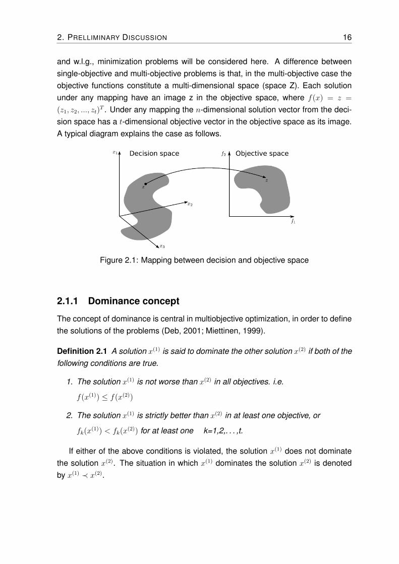
and w.l.g., minimization problems will be considered here. A difference betweensingle-objective and multi-objective problems is that, in the multi-objective case theobjective functions constitute a multi-dimensional space (space Z). Each solutionunder any mapping have an image z in the objective space, where f(x) = z =

(z1, z2, ..., zt)T . Under any mapping the n-dimensional solution vector from the deci-

sion space has a t-dimensional objective vector in the objective space as its image.A typical diagram explains the case as follows.

Figure 2.1: Mapping between decision and objective space

2.1.1 Dominance concept

The concept of dominance is central in multiobjective optimization, in order to definethe solutions of the problems (Deb, 2001; Miettinen, 1999).

Definition 2.1 A solution x(1) is said to dominate the other solution x(2) if both of thefollowing conditions are true.

1. The solution x(1) is not worse than x(2) in all objectives. i.e.

f(x(1)) ≤ f(x(2))

2. The solution x(1) is strictly better than x(2) in at least one objective, or

fk(x(1)) < fk(x

(2)) for at least one k=1,2,. . . ,t.

If either of the above conditions is violated, the solution x(1) does not dominatethe solution x(2). The situation in which x(1) dominates the solution x(2) is denotedby x(1) ≺ x(2).


2.1.2 Pareto Optimality

The solutions of a multiobjective optimization problem are defined using the conceptof dominance.

Definition 2.2 Non-Dominated set: Considering a set of solutions P, the non-dominatedset P ′ contains those solutions that are not dominated by any member of the set P.

When P is the entire set of feasible solutions, the resulting non-dominated setP ′ is called the Pareto-optimal set. The solutions in P ′ are called Pareto-optimalsolutions, or efficient solutions.

2.1.3 Methods for the Solution of Multiobjective Optimization

Several formulations can be used for dealing with multiobjective optimization prob-lems. In this subsection, we present the ones which are relevant for the develop-ments that are presented in this thesis.

2.1.3.1 The Scalarization Method

A multiobjective optimization problem can be approached by combining its multi-ple objectives into one single scalar objective function. This approach is knownas scalarization or weighted sum approach. More specifically, the weighted summethod minimizes a positively weighted convex sum of the objectives, that is, thatrepresents a new optimization problem with a unique objective function. The mini-mizer of this single objective function is an efficient solution for the original multiob-jective problem, i.e. its image belongs to the Pareto curve.

mint∑

k=1

γk · fk(x)

t∑k=1

γk = 1

γk ≥ 0, k = 1, . . . , t

x ∈ S

Particularly we can say that if the γ weight vector is strictly greater than zero,then the minimizer of the problem is a strict Pareto optimum. While in the case ofat least one γk = 0, then the minimizer of the problem may become a weak Paretooptimum.


The result by Geoffrion (1968) states necessary and sufficient conditions in thecase of convexity as: If the solution set S is convex and the t-objectives fk are convexon S, then x∗ is a strictly Pareto optimum if and only if it exists γ such that x∗ is anoptimal solution of problem P (γ). Similarly: If the solution set S is convex and thet objectives fk are convex on S, x∗ is a weakly Pareto optimum if and only if thereexists γ, such that x∗ is an optimal solution of problem P (γ).

If the convexity hypothesis does not hold, then only the necessary condition re-mains valid, i.e., the optimal solutions of P (γ) is strict Pareto optimum if γ > 0 andon the other hand it’s weak Pareto optimum if at least one γ ≤ 0.

2.1.3.2 ε-constraints Method

Another solution technique to multiobjective optimization is the ε-constraints method(Chankong and Haimes, 1983). Here, the decision maker chooses one objectiveout of t to be minimized; the remaining objectives are constrained to be less than orequal to given target values. In mathematical terms, if we let f1(x) to be the objectivefunction chosen to be minimized, we have the following problem:

min f1(x)

fk(x) ≤ εk, for all k ∈ 1, . . . , t

x ∈ S

The solution for this problem is called an weak solution, which may be, underadditional conditions, an efficient solution.

2.2 The Nonlinear Simplex Search

In this section, we present the specific optimization method that will be employed inthe numerical experiments that are conducted in this thesis.

The simplex search method was firstly proposed by Spendley, Hext, and Himsworthin 1962, (Spendley et al. (1962)) and later refined by Nelder and Mead (1965), itis also known as Nelder Simplex Search (NSS) or Downhill Simplex Search. Themethod was introduced for the minimization of multi-dimensional and non-linear un-constrained optimization problems. It is an algorithm based on the simplex algorithmof Spendley et al. (1962)). The geometrical structure of a simplex is composed of(n + 1) points in n dimensions. If any point x of a simplex is taken as the origin,the n other points define vector directions which span the n-dimension vector space


(Durand and Alliot (1999)). By taking successive elementary geometric transforma-tions, the initial simplex converges towards a minimum value at each iteration. Thismethod is carried out by four movements, namely reflection, expansion, contractionand shrinkage in a geometric shape called simplex.

Definition 2.3 A simplex or n-simplex ∆ is a convex hull of a set of n + 1 affineindependent points ∆i (i=1, . . . ,n+1), in some Euclidean space of dimension n.

Definition 2.4 A simplex is called non-degenerated, if and only if, the vectors inthe simplex denote a linearly independent set. Otherwise, the simplex is calleddegenerated, and then, the simplex will be defined in a lower dimension than n.

If the vertices of the simplex are all mutually equidistant, then the simplex is saidto be regular. Thus, in two dimensions, a regular simplex is an equilateral triangle,while in three dimensions a regular simplex is a regular tetrahedron. The conver-gence towards a minimum value at each iteration of Nelder and Mead’s method isconducted by four scalar parameters to control the movements performed in thesimplex: Reflection (α), Expansion (γ), Contraction (β) and shrinkage σ. At eachiteration, the n + 1 vertices ∆i of the simplex represent solutions which are evalu-ated and sorted according to monotonicity value f(∆1) ≤ f(∆2) ≤ . . . ≤ f(∆n+1).In which ∆ = ∆1,∆2, . . .∆n+1 is a set of vertices that define a nondegeneratesimplex. According to Nelder and Mead, these parameters should satisfy:

α > 0, γ > 1, γ > α, 0 < β < 1 and 0 < σ < 1 (2.2)

Actually, there is no method that can be used to establish these parameters. How-ever, the nearly universal choices used in Nelder and Mead’s method (Nelder andMead (1965)) are:

α = 1, γ = 2, β = 0.5 and σ = 0.5 (2.3)

The transformations performed into the simplex by the Nelder and Mead method aredefined as:

1. Reflection: xr = (1 + α)∆c − α∆n+1

2. Expansion: xe = (1 + αγ)∆c − αγ∆n+1

3. Contraction:

a) Outside Contraction: xoc = (1 + αβ)xc − αβ∆n+1


b) Inside Contraction: xic = (1− β)xc + β∆n+1

4. Shrinkage: Each vertex of the simplex is transformed by the geometric shrink-age defined by: ∆i = ∆1 + σ(∆i−∆1), i= 1, . . . , n+1, and the new vertices areevaluated, see figure (2.2).

Where xc = 1n

∑ni=1 ∆i is the centroid of the n best points except ∆n+1, which is the

worst function value and ∆1 is the best solution identified within the simplex. Thefigure (2.2) shows all the possible movements performed by the method.

Figure 2.2: Geometrical representation illustrate all possible movements in the sim-plex performed by the NSS method. This simplex corresponds to an optimizationproblem with two decision variables.

The simplex corresponds to an optimization problem with two decision variables,where ∆1 and ∆3 are the best and worst points respectively. At each iteration, thesimplex is modified by one of the above movements, according to the following rules:

1. If f(∆1) ≤ f(xr) ≤ f(∆n), then ∆n+1 = xr

2. If f(xe) < f(xr) < f(∆1), then ∆n+1 = xe, otherwise ∆n+1 = xr

3. If f(∆n) ≤ f(xr) < f(∆n+1) and f(xoc) ≤ f(xr) then ∆n+1 = xoc


4. If f(xr) ≥ f(∆n+1) and f(xic) < f(∆n+1), then ∆n+1 = xic; otherwise, performshrinkage.

The stopping criteria employed by Nelder and Mead, and commonly adopted inmany optimization problems is defined by:√√√√ 1

n+ 1

n+1∑i=1

(f(∆i)− f)2 ≤ ε (2.4)

In which f = 1n+1

∑n+1i=1 f(∆i) and ε is a predefined constant. When equation (2.4)

satisfies, then ∆c of the smallest simplex can be taken as the optimum point.

Chapter 3

Infeasibility Certificates

In this chapter, some existing approaches for the formulation of infeasibility certifi-cates are presented.

As an optimization model becomes larger and more complex, infeasibility hap-pens more often during the process of model formulation, and it becomes moredifficult to diagnose the problem. A linear program may have thousands of con-straints or even more: which of these are causing the infeasibility and how shouldthe problem be repaired? In the case of nonlinear programs the issue becomesmore complex. The problem may be entirely infeasible or the solver may just havebeen given a poor starting point from which it is unable to reach feasibility.

In modern optimization models, it is necessary to diagnose and repair infeasi-bility in face of the complexity of the models. In the last two decades, algorithmicapproaches have been introduced for the solution of such problems. The followingthree main approaches are used to handle such issues (Greenberg, 1983):

(i) Identification of irreducible subset (IIS) within the larger set of constraints definingthe model. This approach has the property that the IIS is irreducible, but itbecomes feasible if one or more of its constraints are removed. Identifying anIIS permits the modeler to focus attention on a small set of conflicting functionswithin the larger model. Further improvement of the base algorithms try toreturn IISs that are of small cardinality.

(ii) The second approach of analyzing infeasibility is to identify the maximum feasi-ble subset of constraints within the larger set of constraints defining the prob-lem, or the minimum cardinality set of constraints that must be removed so thatthe remainder constitutes a feasible set.

(iii) The third approach seeks to suggest the best repair for the problem, where’best’ can be defined in various ways that can be handled algorithmically, e.g.

23

3. INFEASIBILITY CERTIFICATES 24

the fewest changes to constraint right hand side values. The suggested repaircan of course be accepted, modified or rejected by the modeler.

The above methods for analyzing infeasibility as described above mostly dependon the ability of the solver to determine the feasibility or infeasibility of a problemsubject to an arbitrary set of constraints with very high accuracy. This ability andskills are easily available for a linear problem, but on the other hand it is much moreproblematic for mixed integer and nonlinear problems.

This chapter starts from the result known as Farkas lemma, that certifies that anoptimization problem is indeed infeasible. An easy example deals with the case indetail. The rest of the chapter presents different methods and infeasibility certificatesfor linear and non-linear optimization problems. This part is a gateway to our workwhich is described in the next chapters.

Example 3.1 The linear optimization problem given by:

minimize x1 (3.1)

subject to x1 ≤ 1,

x1 ≥ 2,

This problem is clearly infeasible, i.e. the problem has no solution. In otherwords the problem does not have a solution. To find the possible solution for theabove problem, there are several possible ways to repair the problem. For example,the right hand side of the constraints may be changed appropriately, or one of theconstraints may be removed. In the above simple example it is easy to discover theinfeasibility and figure out a repair. Generally infeasibility problems are much morelarger and complex to figure out it by hand.

3.1 The Farkas’ certificate of primal infeasibility

If (3.1) is feasible, then it will be enough to have a feasible solution x to certify thisclaim. On the other hand, if (3.1) is not feasible, how can somebody claim that itis infeasible? Luckily there exist a well known certificate of infeasibility to answerthis question, known as Farkas’ lemma (Erling D. Andersen, 2011). Lets explain thiscertificate of infeasibility by taking a linear optimization problem.


(P ) minimize cTx (3.2)

subject to Ax = b,

x ≥ 0,

In which b ∈ Rm, A ∈ Rm×n, and c, x ∈ Rn. The problem (3.2) is infeasible if andonly if there exist a y such that

bTy > 0 (3.3)

ATy ≤ 0

In other words any y satisfying (3.3) is a certificate of primal infeasibility. Noticethat it is easy to verify that a Farkas’ certificate y∗ is valid because it corresponds tochecking the conditions

bTy∗ > 0 (3.4)

and

ATy∗ ≤ 0 (3.5)

Which shows that y∗ is a certificate of infeasibility. It is easy to prove that in-deed it is the case. Therefore, if an infeasibility certificate exists, then (3.2) can’tbe a feasible problem since we would have a contradiction of proving them. Thegeneralization of (3.2) is given by

minimize cTx (3.6)

subject to A1x = b1,

A2x ≤ b2,

A3x ≥ b3,

x ≥ 0,

The equation (3.6) is infeasible if and only if there exists a (y1, y2, y3) such that


bT1 y1 + bT2 y2 + bT3 y3 > 0, (3.7)

AT1 y1 + AT2 y2 + AT3 y3 ≤ 0,

y2 ≤ 0,

y3 ≥ 0.

The above generalized Farkas’ certificate of infeasibility for (3.1) is given by

y1 + 2y2 > 0, (3.8)

y1 ≤ 0,

y2 ≥ 0.

And hence the valid certificate for it is y1 = −1 and y2 = 1. It is notable herethat an infeasibility certificate is not unique because if it is multiplied by any strictlypositive number, then it is still a certificate of infeasibility. Actually the infeasibilitycertificate of an optimization problem is a property of it rather than of the algorithm.Therefore it is good enough to request an infeasibility certificate from an algorithmwhenever it claims a problem is infeasible. Since the properties of an infeasibilitycertificate are algorithm independent, decision based on infeasibility certificates willbe similarly algorithm independent.

3.2 Validity of Farkas’ certificate for relaxed

problems

Farkas’ certificate is not only used to certify that an optimization problem is infeasi-ble, it can also be used to find out the case of infeasibility. In common practice if aproblem is infeasible we would like to repair it, or on the other hand to know at leastwhich part of the problem causing infeasibility. For example a simple approach isthe case of problem (3.1). If we change the right-hand of the second constraint to


x1 ≥ 1.2 then the revised Farkas’ conditions are

y1 + 2y2 > 0, (3.9)

y1 ≤ 0,

y2 ≥ 0.

It is still very clear that the previous certificate of infeasibility y1 = −1 and y2 = 1 isstill a valid certificate for the changed problem as well. If we further change the right-hand side of the second constraint to 1, then the Farkas’ certificate of infeasibilityis no longer valid. Generally, when repairing an infeasibility problem it should bechange as much as the infeasibility certificate remain invalid because otherwise theproblem stays infeasible. All yi are non zero in the infeasibility certificate. If anyyi = 0, then the i-th constraint is not involved in the infeasibility since if the i-thconstraint is removed from the problem and yi is removed from the vector y, thenthe reduced y is still an infeasibility certificate.

3.3 Primal or Dual infeasibility in Linear Case

In this section, the certificate of primal and dual infeasibility (Andersen, 2001) isdiscussed. Furthermore, a definition of a basis certificate and strongly polynomialalgorithm of Farkas’ type for the computation of the basis certificate of infeasibilityhave been included.

Generally, if a linear program has an optimal solution, then the certificate of feasi-bility status are the primal and dual optimal solutions. It is well known, in the solvablecases that the linear program must have a basic optimal solution. We know that if alinear program is primal or dual infeasible, then the Farkas lemma (as discussed inthe previous section) provides the basic infeasibility certificate.

Interior-point methods have emerged as an efficient alternative to simplex basedsolution methods for linear programming. Unluckily some of these methods such asthe primal-dual algorithms discussed in (Wright, 1997) do not handle primal or dualinfeasible linear programs very well, but interior-point methods based on the homo-geneous model find a possible infeasible status both in theory and practice (Ander-sen and Andersen, 2000; Roos et al., 1997). In their approach they used Farkas’lemma to generate these infeasibility certificates from the interior-point methods.

Consider problem (3.2). For convenience and without loss of generality the rankof A is assumed as rank(A) = m. The dual problem corresponding to (3.2) is


(D) maximize bTy

subject to ATy + s = c

s ≥ 0,

In which y ∈ Rm and s ∈ Rn. Problem (3.2) is said to be feasible if a solutionthat satisfies the constraints of (3.2) exists. Similarly (D) is said to be feasible if (D)

has at least one solution satisfying the constraints of (D). The following Lemma is awell-known fact of linear programming.

Lemma 3.3.1

a. (P ) has an optimal solution if and only if there exist (x∗, y∗, s∗) such that

Ax∗ = b, ATy∗ + s∗ = c, cTx∗ = bTy∗, x∗, s∗ ≥ 0.

b. (P ) is infeasible if and only if there exists y∗ such that

ATy∗ ≤ 0, bTy∗ > 0. (3.10)

c. (D) is infeasible if and only if there exists x∗ such that

Ax∗ = 0, cTx∗ < 0, x∗ ≥ 0. (3.11)

Proof See (Roos et al., 1997).

Therefore, (P ) has an optimal solution if and only if (P ) and (D) are both feasible.Apart from this, a primal and dual optimal solution is a certificate that the problemhas an optimal solution. If the problem is primal or dual infeasible, then any y∗ satis-fying (3.10) and any x∗ satisfying (3.11) is a certificate of primal and dual infeasibility.A linear programming problem may be both primal and dual infeasible and in thatcase both a certificate for the primal and dual infeasibility exists. It is interesting tonote that, if a linear optimization problem is solved by the method of column gen-eration, and for example the first sub-problem is infeasible, then any column of thissub-problem having a positive inner product with the infeasibility certificate y∗ of pri-mal infeasibility is suitable to be included in the next sub problem. At the end of thissearch, if no such a column exists, then the whole problem can be concluded to beinfeasible with the non-unique infeasibility certificate y∗.


In the following, the definition of an optimal basic partition of the indices of thevariables for a primal infeasible program is taken from (Andersen, 2001) in orderto know that whether an LP has a feasible or an infeasible solution. The phase 1problem corresponding to (3.2) is

maximize z1p = eT t+ + eT t− (3.12)

subject to Ax+ It+ − It− = b,

x, t+, t− ≥ 0.

in which e is a vector of appropriate dimension containing all ones. Problem (3.13)has clearly a feasible solution and the purpose of the objective function in this form isto minimize the sum of infeasibility. The primal problem (3.2) has a feasible solutionif and only if z∗1p = 0. The basic partition (β,N) of the indices of the variables takenfrom (Andersen, 2001) is a certificate of primal infeasibility if it satisfies the followingdefinition.

Definition 3.1 A basic partition (β,N) of the indices of the variables to (3.2) is acertificate of primal infeasibility if

∃i : eTi B−1A ≥ 0, eTi B

−1b < 0 (3.13)

It is notable that any infeasible linear program has a basic partition of the indicesof the variables which satisfies the above definition. The following result is stated in(Andersen, 2001).

Theorem 3.3.2 Given any certificate (y∗, s∗) of primal infeasibility (Andersen andAndersen, 2000), then a basis certificate satisfying definition (3.1) can be computedin strongly polynomial time.

3.4 Infeasibility certificate for monotone

complementarity problem

Andersen and Ye (1999) presented the generalization of a homogeneous self-duallinear programming (LP) algorithm for the solution of monotone complementarityproblem (MCP). Their algorithm generates either a solution converging towards fea-sibility and complementarity or a certificate proving infeasibility of the problem. The


monotone complementarity problem in the standard form is given by

(MCP ) minimize xT s (3.14)

subject to s = f(x), (x, s) ≥ 0

In the above equation f(x) is a continuous monotone mapping i.e. f : Rn+ → Rn,

where Rn+ := x ∈ Rn : x ≥ 0 and x, s ∈ Rn. Equation (3.14) can be written as: for

every x1, x2 ∈ Rn+, we have

(x1 − x2)T (f(x1)− f(x2)) ≥ 0

The problem (3.14) is said to be (asymptotically) feasible if and only if there exista bounded sequence (xt, st) ⊂ R2n

++, t = 1, 2 . . . , such that

limt→∞

st − f(xt) −→ 0,

Any limit point (x, s) of the above sequence is called an (asymptotically) feasi-ble point for the monotone complementarity problem (3.14). Moreover the prob-lem (3.14) has an interior feasible point if it has an (asymptotically) feasible point(x > 0, s > 0). Equation (3.14) is called to be (asymptotically) solvable if there existan (asymptotically) feasible point (x > 0, s > 0) such that xT s = 0, where (x, s) iscalled optimal or the monotone complementarity solution for (3.14). The monotonecomplementarity problem (3.14) is said to be strongly infeasible if and only if thereis no sequence (xt, st) ⊂ R2n

++, t = 1, 2 . . . , such that

limt→∞

st − f(xt) −→ 0,

The monotone complementarity problem (MCP) algorithm (Andersen and Ye,1999) has the following features:

• It achieves O( n√

log(1/ε)) iteration complexity if f satisfies the scaled Lipschitzcondition.

• It solves the problem without any regularity assumption concerning the exis-tence of optimal, feasible, or interior feasible points.

• It can start at a positive point, feasible or infeasible, near the central ray ofthe positive orthant (cone), and it does not need to use any big-M penaltyparameter or lower bound.


• If (MCP) has a solution, the algorithm generates a sequence that approachesfeasibility and optimality simultaneously; if the problem is (strongly) infeasible,the algorithm generates a sequence that converges to a certificate provinginfeasibility.

3.5 Infeasibility certificate in homogenous model for

convex optimization

The previous section was about the certificate of monotone complementarity prob-lem (MCP). The good thing about (MCP) is that it is either solvable or (strongly) infea-sible, which provides a certificate of optimality or infeasibility. In (Andersen, 2000),the suggested formulation of (Andersen and Ye, 1999) is applied to the Karush-Kuhn-Tucker optimality condition corresponding to a homogenous model for convexoptimization problem which provides an infeasibility certificate. This (MCP) corre-sponding certificate provides information about whether the primal or dual problemis infeasible given certain assumptions.

The convex optimization problems have an optimal solution that can be foundby most of the interior point methods. If the problem is primal or dual infeasible,then the optimal solution is not possible. Andersen and Ye (1999) handled this issueand generalized it for the linear problems as a monotone complementarity problem(MCP). This larger class contains all convex optimization problems, because theKarush-kuhn-Tucker conditions corresponding to a convex optimization problemsform an MCP. In the previous section, in the certificate of (Andersen and Ye, 1999),it is not stated whether an infeasibility certificate indicates primal or dual infeasibilitywhen the homogenous model is applied to the optimality conditions of a convexoptimization problem. This issue is handled in (Andersen, 2000), which shows thatan infeasibility certificate in some cases indicates whether the primal or dual problemis infeasible. The optimization problem in (Andersen, 2000) is given by

minimize c(x) (3.15)

subject to ai(x) ≥ 0, i = 1, . . . ,m,

in which x ∈ Rn. The function c : Rn → R is assumed to be convex, and thecomponent function ai : Rn → R, i = 1, . . . ,m, are assumed to be concave. Allfunctions in (3.15) are assumed to be once differentiable. Hence, the problem (3.15)minimizes a convex function over a convex set. The Lagrange function is defined


as:

L(x, y) := c(x)− yTa(x)

The Wolf dual corresponding to (3.15) is defined as

maximize L(x, y) (3.16)

subject to ∇xL(x, y)T = 0

y ≥ 0

The combined equations (3.15) and (3.16) give the MCP

minimize yT z (3.17)

subject to ∇xL(x, y)T = 0

a(x) = z

y, z ≥ 0

in which z ∈ Rm is a vector of slack variables. A solution to (3.17) is said to becomplementarity if the corresponding objective value is zero.

In the following, the homogenous model suggested in (Andersen and Ye, 1997;Andersen, 2000) is applied to this problem, the obtained homogenized MCP is

minimize zTy + τκ (3.18)

subject to τ∇xL(x/τ, y/τ)T = 0,

τa(x/τ) = z

−xT∇xL(x/τ, y/τ)T − yTa(x/τ) = κ,

z, τ, y, κ ≥ 0

in which τ and κ are additional variables. From (Andersen and Ye, 1999), equation(3.18) is said to be asymptotically feasible if and only if a convergent sequence(xk, zk, τ k, yk, κk) exists for k = 1, 2 . . . such that

limk→∞

τ k∇xL(xk/τ k, yk/τ k)T ,

τ ka(xk/τ k)− zk,−(xk)T∇xL(xk/τ k, yk/τ k)T − (yk)Ta(xk/τ k)− τ k

= 0 (3.19)


and

(xk, zk, τ k, zk, κk) ∈ Rn ×Rm+ ×R++ ×Rm

+ ×R++ ∀k, (3.20)

in which the limit point of the (xk, zk, τ k, yk, κk) is called an asymptotically feasiblepoint. Also this limit point is said to be asymptotically complementary if

(y∗)T z∗ + τ ∗κ∗ = 0

Theorem 3.5.1 Equation (3.18) is asymptotically feasible, and every asymptoticallyfeasible point is an asymptotically complementarity solution.

Proof . See (Andersen and Ye, 1997)

This result implies that the objective function (3.18) is redundant, and hence theproblem is a feasibility problem. The following lemma from (Andersen, 2000) possi-bly concludes that either the primal or the dual problem is infeasible.

Lemma 3.5.2 Let (xk, zk, τ k, yk, κk) be any bounded sequence satisfying (3.20) suchthat

limk→∞

(xk, zk, τ k, yk, κk) = (x∗, z∗, τ ∗, y∗, κ∗)

is an asymptotically feasible and maximally complementarity solution to (3.18). Given

limk→∞−(xk)T∇xL(xk/τ k, yk/τ k)T − (yk)Ta(xk/τ k) = κ∗ > 0, (3.21)

then

limk→∞

sup (∇a(xk/τ k)(yk/τ k)− a(xk/τ k))T (yk) > 0 (3.22)

or

limk→∞

sup −∇c(xk/τ k)xk > 0 (3.23)

holds true. Moreover, if

limk→∞

τ k∇c(xk/τ k) = 0, (3.24)

then the primal problem (3.15) is infeasible if (3.22) holds and the dual (3.16) isinfeasible if (3.23) holds.


Proof . (Andersen, 2000)

3.6 Infeasibility detection in Nonlinear Optimization

Problems

Byrd et al. (2010) address the need for optimization algorithms that can solve fea-sible problems and detect when a given optimization problem is infeasible. Forthis purpose an active-set sequential quadratic programming method was proposed,which is derived from an exact penalty approach that adjusts the penalty parameterappropriately to emphasize optimality over feasibility. In this approach, the updatingprocess of penalty parameter is used in every iteration, particularly in the case ofinfeasible problems. The optimization problem in (Byrd et al., 2010) is given by

minx∈Rn

f(x)

s.t. gi(x) ≥ 0, i ∈ I = 1, . . . , t (3.25)

in which f : Rn → R and gi : Rn → R are smooth functions. When there is nofeasible point of (3.25), then the algorithm returns a solution of the problem

minxν(x) ,

∑x∈I

max−gi(x), 0 (3.26)

When problem (3.25) is infeasible, the iterations converge quickly to an infeasiblestationary point x, which is defined as a stationary point of problem (3.26) such thatν(x) ≥ 0. The problem (3.25) is locally infeasible if there is an infeasible stationarypoint x for it. The general form of the Penalty-SQP framework in (Byrd et al., 2010)is given below:

φ(x; ρ) = ρf(x) + ν(x)

in which ν is the infeasibility measure as defined in (3.26) and ρ > 0 is a penaltyparameter updated dynamically within the approach. If the penalty parameter is verysmall, then the stationary points of the non-linear program (3.25) are also stationarypoints of the penalty function φ as in (Han and Mangasarian, 1979). Given a valuefor ρk and an iterate xk, the appropriate step dk is defined as a solution to the sub-problem


minx∈Rn

qk(d; ρk) (3.27)

in which

qk(d; ρk) = ρk∇f(xk)Td+ 1/2dTW (xk, λK ; ρk)d+

∑x∈I

max−gi(xk)

−∇gi(xk)Td, 0 (3.28)

is a local model of the penalty function φ(.; ρ) about xk. W (xk, λk; ρk) is the Hessianmatrix given as follows

W (xk, λk; ρk) = ρk∇2f(xk)−∑x∈I

λik∇2gi(xk) (3.29)

The Hessian used here is different from that used in the standard penalty meth-ods (Nocedal and Wright, 2006) in that the penalty parameter only multiplies theHessian of the objective but not the term involving the Hessian of the constraints.The smooth reformulation of (3.27) is given below

minx∈Rn,s∈Rt

ρk∇f(xk)T + 1/2dTW (xk, λ; ρk)d+

∑i∈I

si (3.30a)

s.t. gi(xk) +∇gi(xk)Td+ si ≥ 0, i ∈ I, (3.30b)

si ≥ 0, i ∈ I, (3.30c)

in which si are slack variables. The sub-problem (3.30) is the focal point of thisapproach which seeks optimality and feasibility with evolution of the value for ρ.With a solution dk to problem (3.30), the iterate is updated as

xk+1 = xk + αkdk

in which αk is a steplength parameter that ensures sufficient reduction in (φ(.; ρk)).The constraints (3.30) are always feasible, which was one of the main motivations

for the Sl1QP approach proposed by Fletcher in 1980s.The rules described by Byrd et al. (2008b) were designed to ensure global con-

vergence (even in the infeasible case) and (Byrd et al., 2003, 2008a) show the ef-


fectiveness in practice. However the problem was that it did not produce a fast rateof convergence in the infeasible case.

Properties for penalty SQP algorithms applied to feasible problems have beenstudied in (Fletcher, 1987), but in (Byrd et al., 2010), the authors focused their anal-ysis on the infeasible case. In the infeasible case, many others like Gill et al. (2002)make no attempt to make a fast rate of convergence to stationary points. For this,Byrd et al. (2010) focused their analysis on the infeasible case for the followingpenalty problem.

minx,r

ρf(x) +∑i∈I

ri

s.t. gi(x) + ri ≥ 0, ri ≥ 0, i ∈ I (3.31)

in which ri are slack variables. If xρ is defined as a first-order optimal solution ofproblem (3.31) for a given value of ρ, then there exist slack variables rρ and Lagrangemultipliers λρ, σρ such that (xρ, λρ, rρ, σρ) satisfy the KKT system

ρ∇f(x)−∑i∈I

λi∇gi(x) = 0, (3.32a)

1− λi − σi = 0, i ∈ I, (3.32b)

λi(gi(x) + ri) = 0, i ∈ I, (3.32c)

σiri = 0, i ∈ I, (3.32d)

gi(x) + ri ≥ 0, (3.32e)

r, λ, σ ≥ 0. (3.32f)

Particularly, if ρ > 0 such a solution has rρ = 0, then xρ is a first order optimalsolution for the non-linear problem (3.25). The following lemma (Byrd et al., 2010) isan alternative way of characterizing solutions of the penalty problem (3.31).

Lemma 3.6.1 Suppose that (xρ, λρ, rρ, σρ) is a primal-dual KKT point for problem(3.31) and that the strict complementarity conditions

rρ + σρ > 0, λρi + (gi(xρ) + rρi ) > 0 (3.33)


hold for all i ∈ I. Then (xρ, λρ) satisfy the system

ρ∇f(x)−∑i∈I

λi∇gi(x) = 0, (3.34a)

and either 1− λi − σi = 0, i ∈ I, (3.34b)

gi(x) < 0, and λi = 1, or (3.34c)

gi(x) > 0, and λi = 0, or (3.34d)

gi(x) = 0, and λi ∈ (0, 1). (3.34e)

Conversely, if (x, λ) satisfy (3.34), it also satisfies (3.32) together with ri = max(0,−gi(x))

and σi = 1− λi

Proof See (Byrd et al., 2010)

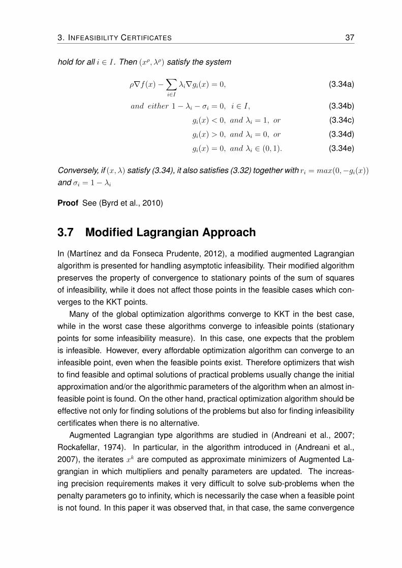
3.7 Modified Lagrangian Approach

In (Martínez and da Fonseca Prudente, 2012), a modified augmented Lagrangianalgorithm is presented for handling asymptotic infeasibility. Their modified algorithmpreserves the property of convergence to stationary points of the sum of squaresof infeasibility, while it does not affect those points in the feasible cases which con-verges to the KKT points.

Many of the global optimization algorithms converge to KKT in the best case,while in the worst case these algorithms converge to infeasible points (stationarypoints for some infeasibility measure). In this case, one expects that the problemis infeasible. However, every affordable optimization algorithm can converge to aninfeasible point, even when the feasible points exist. Therefore optimizers that wishto find feasible and optimal solutions of practical problems usually change the initialapproximation and/or the algorithmic parameters of the algorithm when an almost in-feasible point is found. On the other hand, practical optimization algorithm should beeffective not only for finding solutions of the problems but also for finding infeasibilitycertificates when there is no alternative.

Augmented Lagrangian type algorithms are studied in (Andreani et al., 2007;Rockafellar, 1974). In particular, in the algorithm introduced in (Andreani et al.,2007), the iterates xk are computed as approximate minimizers of Augmented La-grangian in which multipliers and penalty parameters are updated. The increas-ing precision requirements makes it very difficult to solve sub-problems when thepenalty parameters go to infinity, which is necessarily the case when a feasible pointis not found. In this paper it was observed that, in that case, the same convergence


results are obtained using bounded away from zero tolerances for solving the sub-problems. This fact motivates the employment of dynamic adaptive tolerances thatdepend on the degree of infeasibility and complementarity at each iterate xk. Adap-tive precision control for optimality depending on infeasibility measures has beenconsidered, with different purposes. The problem in (Martínez and da Fonseca Pru-dente, 2012) is given by:

Minimize f(x) (3.35)

subject to h(x) = 0

g(x) ≤ 0

x ∈ Ω

in which h : Rn → Rm, g : Rn → Rp, f : Rn → R are smooth and Ω ⊂ Rn is abounded n-dimensional box given by:

Ω = x ∈ Rn | ai ≤ xi ≤ bi ∀ i = 1, . . . , n

The Augmented Lagrangian function given in (Rockafellar, 1974) is defined as:

Lp(x, λ, µ) = f(x) +ρ

2m∑i=1

[hi(x) +λiρ

]2 +

p∑i=1

[max(0, gi(x) +µiρ

)]2

for all x ∈ Ω, ρ > 0, λ ∈ Rm, µ ∈ Rp+

This algorithm (Martínez and da Fonseca Prudente, 2012) is similar to the onein (Andreani et al., 2007), but the difference is in the stopping criterion for the sub-problem. The original algorithm imposes that the convergence tolerance εk for thesub-problems should tend to zero while this condition on stopping criteria is relaxedin (Martínez and da Fonseca Prudente, 2012).

Chapter 4

A new Certificate of Infeasibility forNon-linear Optimization Problems

In this chapter we propose a new necessary condition for the infeasibility of non-linear optimization problems which is stated as Pareto-criticality condition of an aux-iliary multiobjective optimization problem.

4.1 Preliminary Statements

Consider the optimization problem defined by:

minxf(x)

subject to: g(x) ≤ 0(4.1)

in which f(·) : Rn 7→ Rp and g(·) : Rn 7→ Rm are vector functions. The set of feasiblepoints is denoted by

Ω , x ∈ Rn | g(x) ≤ 0 (4.2)

In particular case if p = 1, the problem (4.1) is a conventional mono-objective op-timization problem. When p > 1 the problem becomes multi-objective. In this lastcase, a feasible point x ∈ Rn of the decision variable space is said to be dominatedby another feasible point x ∈ Rn if f(x) ≺ f(x). The solution set of the multiob-jective optimization problem is defined as the set P ⊂ Ω of feasible points that arenot dominated by any other feasible point. This set is called the efficient solutionset, or the Pareto-optimal set. In order to state general results, the solution set of amono-objective problem is also denoted by P.

The following compactness assumption will be necessary for the derivation ofour results:

40

4. A NEW CERTIFICATE OF INFEASIBILITY FOR NON-LINEAR OPTIMIZATIONPROBLEMS 41

Assumption 4.1.1 Assume that there is a subset of the constraint functions, g1(·), g2(·), . . . , gk(·),with k ≤ m, such that the set Ωc ⊂ Rn defined by

Ωc = x | g1(x) ≤ 0, g2(x) ≤ 0, . . . , gk(x) ≤ 0

is a non-empty compact set. ♦

This assumption holds in a large class of problems, for instance when there isa “box” in the decision variable space in which the search is to be conducted. Theissue of feasibility/infeasibility can become a difficult question only w.r.t. the otherconstraint functions, gk+1(·), . . . , gm(·).

4.2 Infeasibility Condition

Let λ ∈ Rp and µ ∈ Rm. The Kuhn-Tucker conditions for efficiency at a solution x ofproblem (4.1) is stated as (Luc, 1988; Marusciac, 1989):

(KTE)

F (x)λ+G(x)µ = 0

λ 0 , µ ≥ 0

g(x) ≤ 0

µi gi(x) = 0 ; ∀ i = 1, . . . ,m

(4.3)

Notice that the Karush-Kuhn-Tucker conditions for optimality of the single-objectivecase is a particular case of KTE.

For problem (4.1), given a point x ∈ Rn, one of the four possibilities below musthappen (by exhaustion):

(a) x ∈ P, it means that the Kuhn-Tucker necessary conditions for Efficiency (KTE)hold

(b) x ∈ Λ, with Λ defined as the set of points for which hold:

(INF)

∃ i | gi(x) > 0

G(x)µ = 0

µ 0

gj(x) < 0 ⇒ µj = 0

(4.4)

for some vector of multipliers µ ∈ Rm.

(c) x ∈ Ω and x 6∈ P.

(d) x 6∈ Ω and x 6∈ Λ.


Points that satisfy the condition (KTE) are Pareto-critical for problem (4.1). Thecondition (INF) is very similar to (KTE). It will be shown that points that satisfy (INF)are also Pareto-critical w.r.t. another auxiliary problem. For this we define the fol-lowing vector function g(·) : Rn 7→ Rm as follows:

gi(x) =

0 , ∀ x | gi(x) ≤ 0

gi(x) , ∀ x | gi(x) > 0

i = 1, . . . ,m

(4.5)

The following unconstrained auxiliary problem is defined:

minxg(x) (4.6)

and the corresponding efficient solution set of this problem is denoted by A:

A = x ∈ Rn | 6 ∃ x ∈ Rn such that g(x) ≺ g(x) (4.7)

In the case of feasibility of problem (4.1), the efficient solution setA have feasible so-lution points only. On the other hand, if (4.1) is strictly infeasible then A is composedon those points for which the INF condition holds.

It should be noticed that, under assumption 4.1.1, it can be stated that: A 6= ∅and A ⊂ Ωc. Denote by g(A) the image set of function g(·) over A. The followinglemma comes directly from the definition of the function g(·):

Lemma 4.2.1 The following statements hold:

(i) Ω 6= ∅ ⇒ g(A) ≡ 0 , Ω ≡ A

(ii) Ω = ∅ ⇒ g(x) 0 ∀ x ∈ A

♦

The next lemma states a relation between the set Λ and the set A.

Lemma 4.2.2 The following statement holds:

Ω = ∅ ⇒ Λ ⊃ A

♦

Proof The condition (INF), which holds for the points of Λ, corresponds to the KTE neces-sary condition for the Pareto-optimality w.r.t. problem (4.6) when problem (4.1) is infeasible,which holds for the points of A.


Under convexity assumption, a stronger result can be obtained as:

Lemma 4.2.3 Suppose that the functions f(·) : Rn 7→ Rp and g(·) : Rn 7→ Rm areconvex. In this case, the following statements hold:

(i) Ω = ∅ ⇒ Λ ≡ A

(ii) Ω 6= ∅ ⇒ Λ = ∅

♦

Proof Both statements come from the fact that A is the Pareto-optimal set of the auxiliaryproblem (4.6), which means that the points in this set must satisfy a Pareto-criticality con-dition for this problem. If the problem (4.1) is infeasible, as in case (i), the Pareto-criticalitycondition becomes (INF). In this case, the problem convexity leads to the sufficiency of thePareto-criticality for a point to belong to A. Otherwise, in case (ii), the Pareto-criticality con-dition only holds for feasible points (see Lemma 4.2.1-(i)), and (INF) does not hold for anypoint.

The following Corollary of Lemmas 4.2.1 and 4.2.2 can be stated, without as-suming convexity:

Corollary 4.2.4 Consider any point x ∈ Rn. The following relations hold:

(i) x ∈ (Λ ∩ A)⇒ Ω = ∅

(ii) Ω = ∅ ⇒ (Λ ∩ A) 6= ∅

♦

It should be noticed that the verification of criticality condition x ∈ Λ depends onlyon local gradient evaluation on point x. On the other hand, the efficiency conditionx ∈ A has a global meaning, and cannot be evaluated on the basis of local informa-tion only. However, an assumption of convexity leads to an equivalence of criticalityand efficiency. In this way, the following Corollary of Lemmas 4.2.1 and 4.2.3 holdsunder convexity:

Corollary 4.2.5 Consider any point x ∈ Rn. Suppose that the functions f(·) : Rn 7→Rp and g(·) : Rn 7→ Rm are convex. The following relations hold:

(i) x ∈ Λ⇒ Ω = ∅

(ii) Ω = ∅ ⇒ A = Λ 6= ∅

♦


The main result of this work is stated, in the version without convexity, as theconjunction of the Lemmas 4.2.1, 4.2.2 and Corollary 4.2.4:

Theorem 4.2.6 Consider the optimization problem defined by (4.1). Then:

A = Ω 6= ∅ ⇔ (Λ ∩ A) = ∅

(A ∩ Λ) 6= ∅ ⇔ Ω = ∅(4.8)

♦

The stronger version of this theorem, assuming convexity, is the conjunction ofthe Lemmas 4.2.1, 4.2.3 and Corollary 4.2.5:

Theorem 4.2.7 Consider the optimization problem defined by (4.1), and assumethat the functions f(·) : Rn 7→ Rp and g(·) : Rn 7→ Rm are convex. Then:

A = Ω 6= ∅ ⇔ Λ = ∅

A = Λ 6= ∅ ⇔ Ω = ∅(4.9)

♦

As a consequence of theorem 4.2.7, valid for the convex case, the search for apoint inside the feasible set Ω of problem (4.1) can be stated as a multiobjective op-timization on the auxiliary problem (4.6), which performs a search for Pareto-criticalpoints xa ∈ A. Once any point xa ∈ A has been found, there are two possibilities: (i)xa ∈ Ω, or (ii) xa ∈ Λ. At this point, either xa is feasible, or a certificate of infeasibilityhas been found.

Chapter 5

Results and Discussions

This chapter deals with the numerical implementation of the proposed infeasibilitycertificate.

5.1 Verification of INF Condition

In this work, we applied a scalarization strategy for solving the auxiliary problemwhich is related to the infeasibility certificate. A mathematical programming methodis employed for finding a Pareto optimal solution.

5.1.1 Noise-free problems

First, consider the usual situation of noise-free problems (problems for which it ispossible to obtain gradient information), which is the traditional setting of optimiza-tion problems. This means that it will be possible to calculate the function deriva-tives, which will allow the definition of gradient-based tests. In order to implementthe search for a point xa inside the set A leading either to a feasible point or to acertificate of infeasibility, it is enough to find a single Pareto-optimal solution to theauxiliary problem. A scalarized version of the multi-objective auxiliary problem (4.6)

is stated as:

minx

maxiwi gi(x) (5.1)

Each optimal solution of (5.1) is a Pareto-optimal solution of (4.6). For each Paretooptimal point x there exists a weight vector wi such that x is the optimum solutionof (5.1). The meaning of the solutions of problem (5.1), in its non-convex flavor, isstated as:

46

5. RESULTS AND DISCUSSIONS 47

Theorem 5.1.1 Consider a solution xa of problem (5.1). Then:

xa 6∈ Ω⇒ Ω = ∅ (5.2)

♦

Under the assumption of convexity:

Theorem 5.1.2 Consider a solution xa of problem (5.1). Then:

xa ∈ Ω⇔ Ω 6= ∅ (5.3)

♦

To check the feasibility or infeasibility of the original problem on the basis of thissolution, it is necessary to check the conditions described in section 4.2. If theobtained solution x is feasible, then the feasibility problem is solved. Otherwise, if xsolution is infeasible, it is necessary to check the INF conditions numerically on x.Define:

G(x) =[∇g1 ∇g2 . . . ∇gk

](5.4)

in which k denotes the number of violated constraints in point x, which were as-sumed to occupy the first k indices of the constraint set, w.l.g.. Suppose x ∈ Λ, thenit comes from equation (4.4):

G(x) µ = 0 (5.5)

Suppose w.l.g. that ∇g1 6= 0, and assume that µ1 = 1. Then:

[∇g2 . . . ∇gk

] µ2

...µk

= −∇g1 (5.6)

Now, assume provisionally that matrix H =[∇g2 . . . ∇gk

]has full column rank.

The case in which n = k − 1 leads to a straightforward solution:µ2

...µk

= −[∇g2 . . . ∇gk

]−1∇g1 (5.7)


In the case of n > k − 1 a least-squares solution can be expressed as:µ2

...µk

= −([∇g2 . . . ∇gk

]T [∇g2 . . . ∇gk

])−1 [∇g2 . . . ∇gk

]T∇g1

(5.8)In both cases, if all the components of µ given by equations (5.7) and (5.8) are

positive, then the condition (INF) will hold and the problem will be strictly infeasible.On the other hand, if there is at least one negative multiplier, it is not possible to de-clare that the original problem is infeasible. In order to remove the assumption of fullcolumn rank of H, consider the submatrices composed by subsets of the columnsof H, such that they attain the largest possible column rank. All such matrices canbe evaluated, using the suitable criterion, either (5.7) or (5.8). If the INF condition isverified for any such a matrix, then the problem can be declared to be infeasible.

Now, in the case of n < k − 1,

[∇g1 ∇g2 . . . ∇gk

]µ1

µ2

...µk

= 0 (5.9)

which means that µ ∈ N (G), in which N (·) stands for the null space of the argumentmatrix. Let K+ denote the cone of the positive octant of suitable dimension. In thiscase, if

N (G) ∩ K+ 6= 0 (5.10)

then the condition (INF) will hold, and the problem will be strictly infeasible.

5.1.2 Noisy problems

Now, consider the situation of noisy problems, in which the function values are sup-posed to be corrupted by some noise. In this case, the computation of derivativesshould be avoided, since the noise would be amplified in that computation. In thissituation, the proposed indicator is still suitable for providing an infeasibility certifi-cate. The kind of evidence to be employed, in this case, relies on the description ofthe Pareto-front of the auxiliary problem (4.6) (the image of the set A, in the spaceof constraint function values), denoted by g(A). The following theorem states thefacts that support the proposed procedure.

Theorem 5.1.3 Let y = g(x) for some x ∈ A. The following statements hold:


(i) y ≺ 0 ⇒ x ∈ Ω

(ii) 0 ≺ y ⇒ Ω = ∅

♦

The reasoning that was implicit, in the former subsection, was that: (i) An op-timization algorithm should be executed in order to solve problem (5.1). (ii) Afterthe solution is found, if it is not feasible, a criticality test is performed, in order toensure that it is indeed a solution. Once the criticality test returns a positive answer,the (INF) condition is considered to hold, and the infeasibility of the problem (4.1) isdeclared.

Now, in order to replace the criticality test as the additional evidence that sup-ports the declaration of infeasibility of problem (4.1), it is adopted a regularity test.

Definition 5.1 Let F denote the intersection of the Pareto-front of 4.6 with the pos-itive orthant of the space of constraint function values:

F = g(A) ∩ K+ (5.11)

Let C(F) denote the convex hull of F , and let ∂C(F) denote the boundary of the setC(F). The surface F is said to be regular if:

(i) It has no holes.

(ii) Every point y ∈ F belongs to ∂C(F).

♦

Of course, the regularity is not a necessary attribute of F . However, the features(i) and (ii) are rather usual in the context of constraint functions. Therefore, theregularity provides support to the declaration of infeasibility of problem (4.1).

The regularity test procedure is stated as:

(a) Find a description of the Pareto-front of the auxiliary problem (4.6) in the positiveorthant.

(b) If such a description is consistent with a regular Pareto-front surface, then de-clare that the (4.1) is infeasible.

Step (a) should be performed using a derivative-free multiobjective optimizationalgorithm. For this purpose, the evolutionary multiobjective algorithms are well-suited. For instance, the NSGA-II algorithm (Deb et al., 2002) and the SPEA-2


algorithm (Zitzler et al., 2002) both provide suitable mechanisms for producing auniform sampling of F . However, for problems with a large number of constraintfunctions, a better choice would be a decomposition-based evolutionary algorithm,such as MOEA-D (Zhang and Li, 2007), due to the many-objective degradation ef-fect on algorithms that use Pareto-based selection (such as NSGA-II or SPEA-2).

Step (b) can be performed according to the following steps: (i) The existenceof holes is tested with the use of a goal attainment scalarization, defining a testdirection pointing to the region in which there could be a hole. If a new point isfound by this procedure, there is no hole, and the point is added to the Pareto-setsampling. Otherwise, there is a hole, and the surface is not regular. (ii) The conditionthat every point belonging to the Pareto-front sample also belongs to the boundaryof its convex hull is tested by verifying if every point has a hyperplane that separatesit from the other ones.

If step (b) finishes with a positive answer about the regularity of the F surface,the problem (4.1) is declared infeasible.

5.2 Illustrative Examples

In order to perform computational tests involving the proposed infeasibility condition,a simple computational framework has been defined. Since problem (5.1) is a singleobjective problem involving non-differentiable functions, the Non-linear Nelder-MeadSimplex Method Nelder and Mead (1965) can be used to solve it, as discussed inchapter two. For this purpose, a random starting point x0 is considered. The non-linear programming problem results into a solution x. Finally, the obtained solutionx is checked for the infeasibility certificate.

Here, the proposed algorithm is explained graphically with the help of some sim-ple examples. Each example show that the problem is feasible or strictly infeasibleat the solution point x and consequently the obtained solutions belong to the feasibleset Ω or to the set of points Λ respectively.

Example 5.1 Consider the following optimization problem with three constraints:

minxf(x)

subject to:

g1(x) = −x1 + x22 ≤ 0

g2(x) = x12 + 3x2

2 − 4 ≤ 0

g3(x) = x12 + (x2 − 5)2 − 4 ≤ 0


In this example, f(x) could be a single or multiobjective function.For this, we can define the vector function like (4.5) as follows;

gi(x) =

0 , ∀ x | gi(x) ≤ 0

gi(x) , ∀ x | gi(x) > 0

i = 1, . . . , 3

From the above vector function, the following auxiliary problem is defined as:

minxg(x)

The auxiliary problem for the above example is given by

minxg(x) = min

g1(x)

g2(x)

g3(x)

Using minmax formulation we have

minx

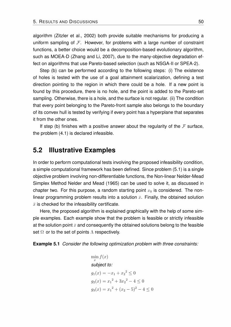
maxiwigi(x)

Applying Nelder Mead Simplex method to solve this minmax problem, we getdifferent solutions depending on the values of weights wi. In the following figure, thedense area shows the INF solutions of this problem.

Figure 5.1: Pareto critical solutions of the problem

This problem is strictly infeasible with trade off solutions near to the boundariesof the constraints.


Example 5.2 Consider the same example with the first two constraints:

minxf(x))

Subject to:

g1(x) = −x1 + x22 ≤ 0

g2(x) = x12 + 3x2

2 − 4 ≤ 0

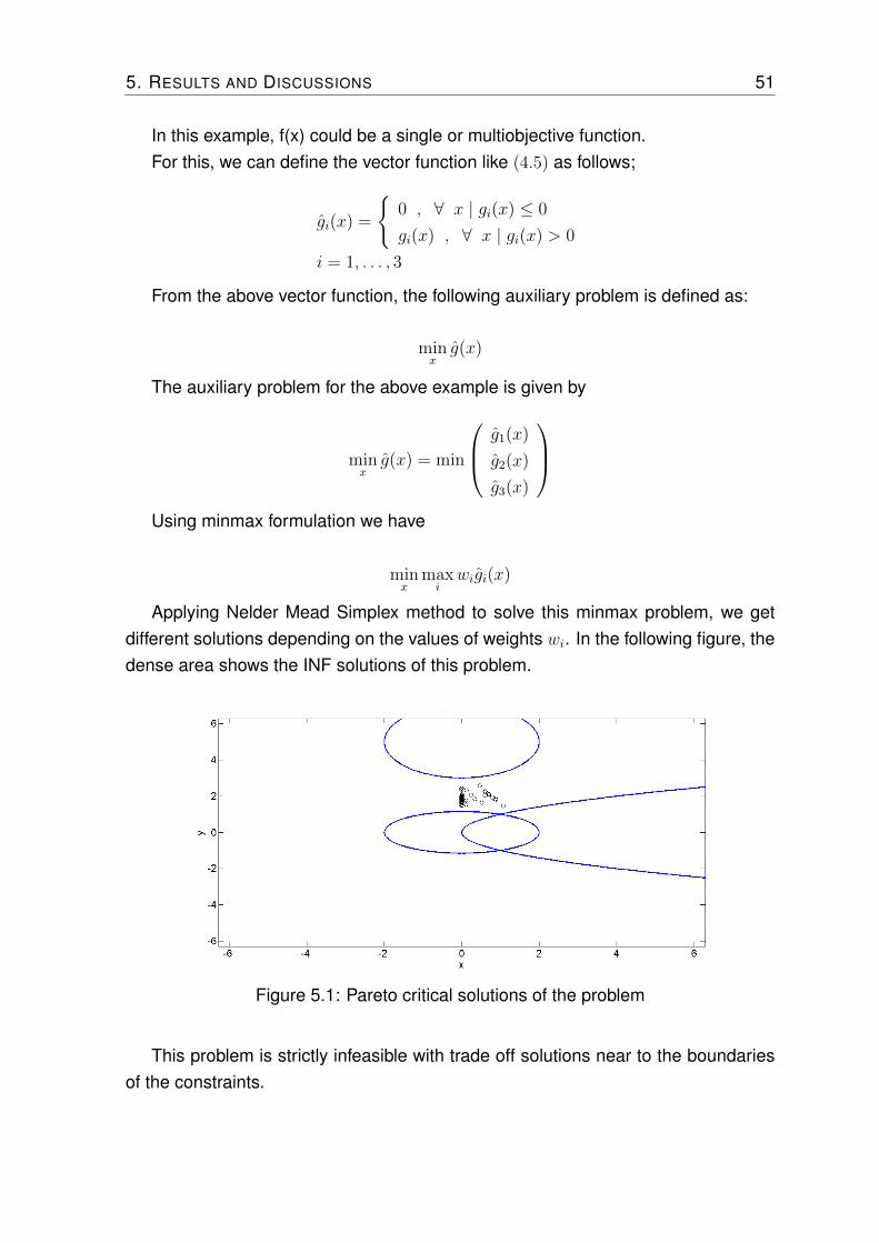
Applying the same procedure as in the previous example, we have the followingfigure.

Figure 5.2: Shows a single feasible solution of the problem

Figure (5.2), shows that the problem is feasible and we end up with one feasiblesolution. Here we can write A = Ω 6= ∅ and Λ = ∅

Example 5.3 Consider the same example with the last two constraints.

minxf(x)

subject to:

g2(x) = x12 + 3x2

2 − 4 ≤ 0

g3(x) = x12 + (x2 − 5)2 − 4 ≤ 0

Figure 5.3 shows a beam of INF solutions, and consequently the problem isstrictly infeasible again.


Figure 5.3: The dense area in the figure shows a beam of INF solutions.

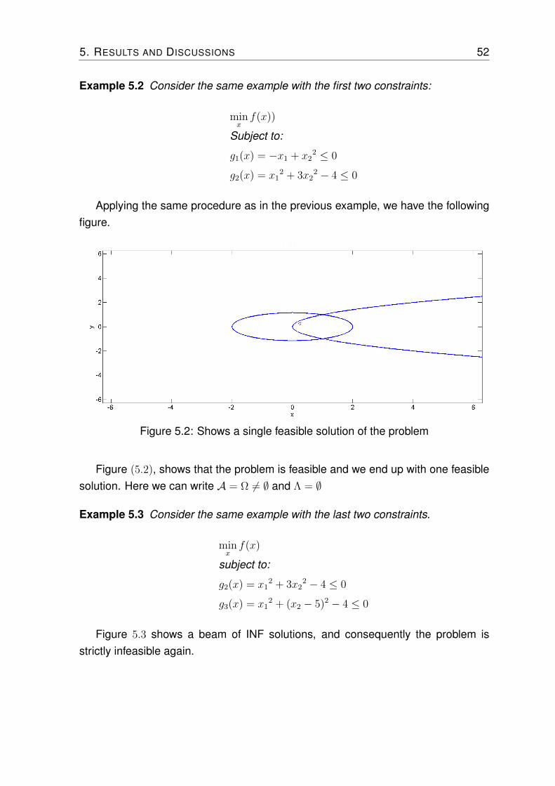
Example 5.4 Consider the following optimization problem taken from (Byrd et al.,2010) with four constraints:

minxf(x)

subject to:

g1(x) = x12 + x2 + 1 ≤ 0

g2(x) = x12 + x2 + 1 ≤ 0

g3(x) = −x12 + x22 + 1 ≤ 0

g4(x) = x1 + x22 + 1 ≤ 0

Figure 5.4 shows that the problem is strictly infeasible with four objective func-tions.

5.3 Algorithms

The whole computational procedure is summarized in the following algorithms.


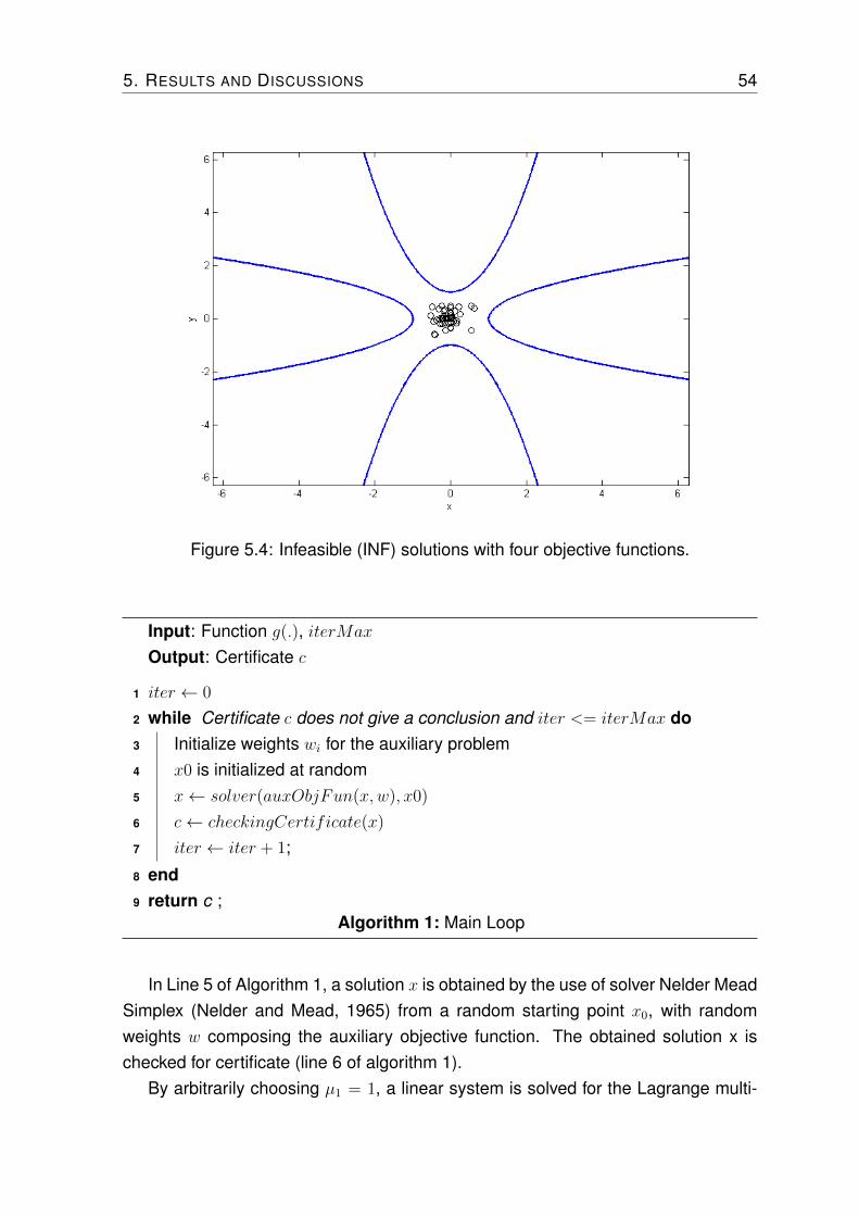
Figure 5.4: Infeasible (INF) solutions with four objective functions.

Input: Function g(.), iterMax

Output: Certificate c

1 iter ← 0

2 while Certificate c does not give a conclusion and iter <= iterMax do3 Initialize weights wi for the auxiliary problem4 x0 is initialized at random5 x← solver(auxObjFun(x,w), x0)

6 c← checkingCertificate(x)

7 iter ← iter + 1;

8 end9 return c ;

Algorithm 1: Main Loop

In Line 5 of Algorithm 1, a solution x is obtained by the use of solver Nelder MeadSimplex (Nelder and Mead, 1965) from a random starting point x0, with randomweights w composing the auxiliary objective function. The obtained solution x ischecked for certificate (line 6 of algorithm 1).

By arbitrarily choosing µ1 = 1, a linear system is solved for the Lagrange multi-


pliers. If all the Lagrange multipliers are greater than 0 then the solution x will resultinto an infeasible certificate.

5.4 Performance on Test Problems

The proposed algorithm was implemented in MATLAB (2013). Computational exper-iments were carried out on a Pentium Core 2 Quad (Q6600) computer with 8GB ofRAM and operating system of Windows 7. The algorithm is tested on five examplesas introduced in Section 5.2 on a batch of different number of executions for eachinstance. The initial points were selected at random.

The computational results of batches of 30 executions are given in Tables 5.1, 5.2and 5.3 for four different scenarios, with maximum number of iterations (iterMax)equal to 30, 50, 200 and 500. In the tables of computational results, lines “FC”and “IC” indicate the number of feasibility and infeasibility certificates obtained foreach problem. Line “NC” indicates the number of iterations in which any certificate isobtained. Line “#x” indicates the average number of solutions obtained for achievingthe feasibility or infeasibility certificates for each example.

Example 5.5 Consider the following example with 6 constraints.

minxf(x)

Subject to:

g1(x) = x21 − x2 + 1 ≤ 0

g2(x) = x21 − x42 ≤ 0

g3(x) = 2x21xexpx12 − x42 ≤ 0

g4(x) = −x1 + x22 ≤ 0

g5(x) = x21 + (x2 − 5)2 − 4 ≤ 0

g6(x) = x21 + 3x22 − 4 ≤ 0


Example 5.6 Consider the following example with 7 constraints.

minxf(x)

Subject to:

g1(x) = xx34 ex4 ≤ 0

g2(x) = +x21 + x2 + x53 + x24 + 1 ≤ 0

g3(x) = x21 − x42 ≤ 0

g4(x) = 2x21xexpx42 − x42 ≤ 0

g5(x) = −x1 + x22 ≤ 0

g6(x) = x21 + (x3 − 5)2 − 4 ≤ 0

g7(x) = x21 + 3x22 − 4 ≤ 0

Finally, three more examples are included in order to further validate the pro-posed algorithm. These quadratic examples are taken from Byrd et al. (2010) having2, 4 and 5 constraints respectively, and so-known as example 1, 3 and 5, and calledin this thesis as Byrd 1, 2 and 3 respectively.

Table 5.1: Computational results for maximum 30 iterations

Ex. 5 Ex. 6 Byrd 1 Byrd 2 Byrd 3FC 0 0 0 0 0IC 0 6 30 28 30NC 30 24 0 2 0#x 3,00 2,90 1,00 1,86 1,00

Table 5.2: Computational results for maximum 50 iterations

Ex. 5 Ex. 6 Byrd 1 Byrd 2 Byrd 3FC 0 0 0 0 0IC 15 29 30 30 30NC 15 1 0 0 0#x 36,93 13,83 1,00 2,03 1,00

Analyzing tables 5.1, 5.2 and 5.3 it can be seen that the proposed algorithmis capable to provide feasibility or infeasibility certificates for the given maximumnumbers of iterations. When the number of iteration is 30 i.e. iterMax = 30, thealgorithm produces 100% of accuracy for instances Byrd 1 and Byrd 3. Considering50 iterations, the algorithm results into 50% of its executions in infeasibility for Ex.5and this percentage is 99% in case of example Ex.6. Table 5.3 is considered for 500


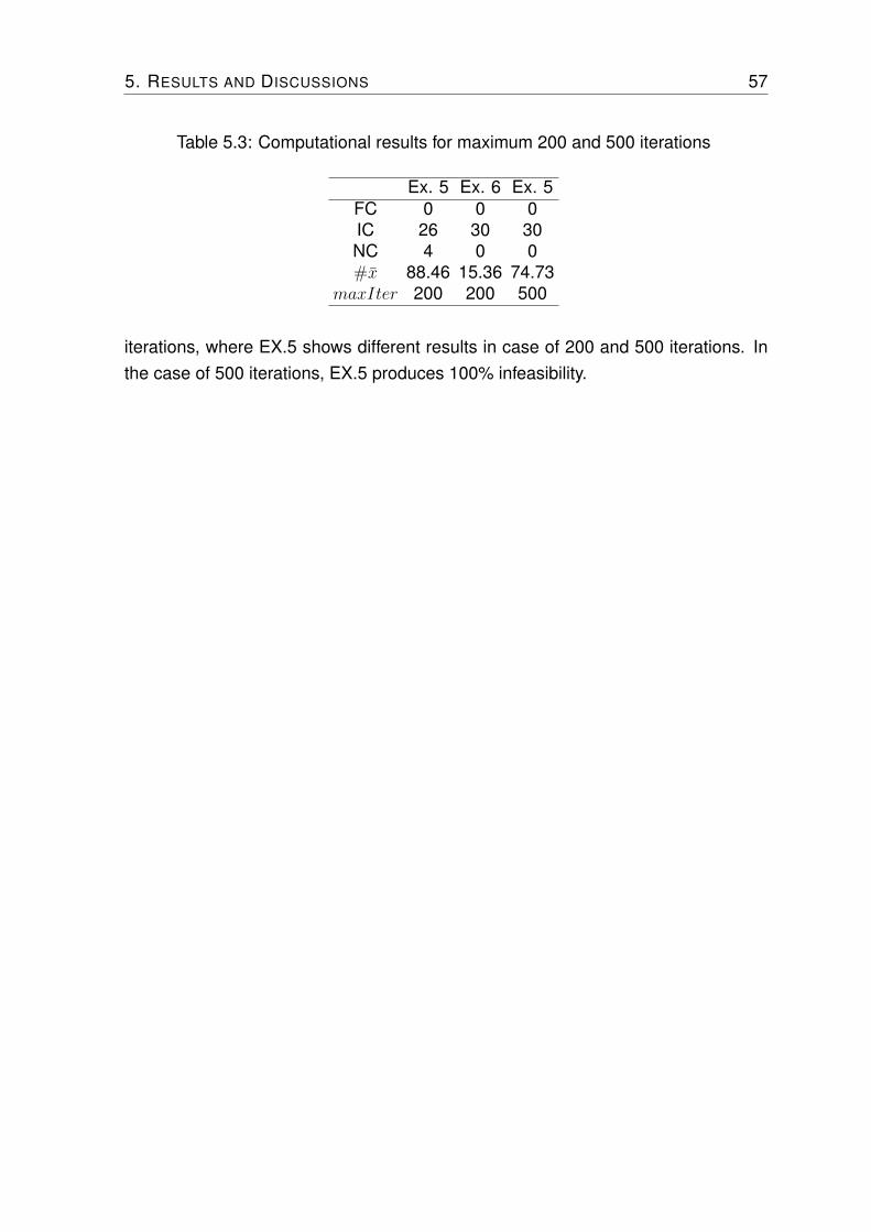
Table 5.3: Computational results for maximum 200 and 500 iterations

Ex. 5 Ex. 6 Ex. 5FC 0 0 0IC 26 30 30NC 4 0 0#x 88.46 15.36 74.73

maxIter 200 200 500

iterations, where EX.5 shows different results in case of 200 and 500 iterations. Inthe case of 500 iterations, EX.5 produces 100% infeasibility.

Chapter 6

Conclusion

In this thesis, a new infeasibility certificate for non-linear optimization problems onthe basis of Pareto-criticality condition of an auxiliary multiobjective optimizationproblem was developed. The main result presented here is a new necessary con-dition (that becomes necessary and sufficient under convexity assumptions) for theinfeasibility of finite-dimensional optimization problems, which is related to the Kuhn-Tucker conditions for efficiency in multi-objective problems. By defining a suitableauxiliary vector function, the search for the feasible set can be stated as the searchfor a point that is Pareto-critical for such an auxiliary problem. Once a Pareto-criticalpoint w.r.t. the auxiliary problem is found, it is either a feasible solution of the orig-inal problem or brings a certificate of infeasibility (which is globally valid for convexproblems). Differently from other existing certificates of infeasibility, the proposedone relies on primal variables only.

Another important difference of the proposed methodology is that it admits amodified version that does not rely on gradient information. In this case, the criticalitytest is replaced by a heuristic regularity test.

The performance of the proposed methodology was tested on some functions,and it delivered promising results.

59

Bibliography

Andersen, E. D. (2000). On primal and dual infeasibility certificates in a homoge-neous model for convex optimization. SIAM Journal on Optimization, 11(2):380–388.

Andersen, E. D. (2001). Certificates of primal or dual infeasibility in linear program-ming. Computational Optimization and Applications, 20(2):171–183.

Andersen, E. D. and Andersen, K. D. (2000). The MOSEK interior point optimizer forlinear programming: an implementation of the homogeneous algorithm. In HighPerformance Optimization, pages 197–232. Springer.

Andersen, E. D. and Ye, Y. (1997). On a homogeneous algorithm for a monotonecomplementarity problem with nonlinear equality constraints. In Complementarityand Variational Problems: State of the Art, pages 1–11. SIAM Philadelphia, PA.

Andersen, E. D. and Ye, Y. (1999). On a homogeneous algorithm for the monotonecomplementarity problem. Mathematical Programming, 84(2):375–399.

Andersen, K., Louveaux, Q., and Weismantel, R. (2008). Certificates of linear mixedinteger infeasibility. Operations Research Letters, 36(6):734–738.

Andreani, R., Birgin, E. G., Martínez, J. M., and Schuverdt, M. L. (2007). On aug-mented Lagrangian methods with general lower-level constraints. SIAM Journalon Optimization, 18(4):1286–1309.

Ben-Tal, A. and Nemirovskiı, A. S. (2001). Lectures on Modern Convex Optimization:analysis, algorithms, and engineering applications. SIAM.

Benson, H. Y., Vanderbei, R. J., and Shanno, D. F. (2002). Interior-point methods fornonconvex nonlinear programming: Filter methods and merit functions. Compu-tational Optimization and Applications, 23(2):257–272.

Byrd, R. H., Curtis, F. E., and Nocedal, J. (2010). Infeasibility detection and SQPmethods for nonlinear optimization. SIAM Journal on Optimization, 20(5):2281–2299.

61

REFERENCES 62

Byrd, R. H., Gould, N. I., Nocedal, J., and Waltz, R. A. (2003). An algorithm fornonlinear optimization using linear programming and equality constrained sub-problems. Mathematical Programming, 100(1):27–48.

Byrd, R. H., Lopez-Calva, G., and Nocedal, J. (2008a). A line search penalty methodfor nonlinear optimization. Technical report, Technical Report 08/05, OptimizationTechnology Center, Northwestern University.

Byrd, R. H., Nocedal, J., and Waltz, R. A. (2006). Knitro: An integrated packagefor nonlinear optimization. In Large-scale nonlinear optimization, pages 35–59.Springer.

Byrd, R. H., Nocedal, J., and Waltz, R. A. (2008b). Steering exact penalty methodsfor nonlinear programming. Optimization Methods and Software, 23(2):197–213.

Chankong, V. and Haimes, Y. (1983). Multiobjective Decision Making: theory andmethodology. Noth-Holland.

Deb, K. (2001). Multi-objective Optimization Using Evolutionary Algorithms, vol-ume 16. John Wiley & Sons.

Deb, K., Pratap, A., Agarwal, S., and Meyarivan, T. (2002). A fast and elitist multiob-jective genetic algorithm: NSGA-II. Evolutionary Computation, IEEE Transactionson, 6(2):182–197.

Durand, N. and Alliot, J.-M. (1999). A combined Nelder-Mead simplex and geneticalgorithm. In GECCO’99: Proceedings of the Genetic and Evolutionary Compu-tation Conference, pages 921–928.

Erling D. Andersen, M. A. (2011). How to use Farkas’ lemma to say somethingimportant about infeasible linear problems.

Fletcher, R. (1987). Practical Methods of Optimization. Wiley.

Fletcher, R., Gould, N. I., Leyffer, S., Toint, P. L., and Wächter, A. (2002). Globalconvergence of a trust-region SQP-filter algorithm for general nonlinear program-ming. SIAM Journal on Optimization, 13(3):635–659.

Geoffrion, A. M. (1968). Proper efficiency and the theory of vector maximization.Journal of Mathematical Analysis and Applications, 22(3):618–630.

Gill, P. E., Murray, W., and Saunders, M. A. (2002). SNOPT: An SQP algorithm forlarge-scale constrained optimization. SIAM Journal on Optimization, 12(4):979–1006.

REFERENCES 63

Greenberg, H. (1983). A functional description of ANALYZE: A computer-assistedanalysis system for linear programming models. ACM Transactions on Mathemat-ical Software (TOMS), 9(1):18–56.

Han, S.-P. and Mangasarian, O. L. (1979). Exact penalty functions in nonlinearprogramming. Mathematical programming, 17(1):251–269.

Luc, D. T. (1988). Theory of Vector Optimization. Springer-Verlag, Berlin.

Martínez, J. M. and da Fonseca Prudente, L. (2012). Handling infeasibility in a large-scale nonlinear optimization algorithm. Numerical Algorithms, 60(2):263–277.

Marusciac, I. (1989). On Fritz-John-type optimality criterion in multi-objective opti-mization. Revue d ’Analyse Numerique et de Theorie de l’Approximation, 11:109–114.

MATLAB (2013). version 7.10.0 (R2013a). The MathWorks Inc., Natick, Mas-sachusetts.

Miettinen, K. (1999). Nonlinear Multiobjective Optimization. Springer.

Nelder, J. A. and Mead, R. (1965). A simplex method for function minimization. TheComputer Journal, 7(4):308–313.

Nesterov, Y., Todd, M., and Ye, Y. (1999). Infeasible-start primal-dual methods andinfeasibility detectors for nonlinear programming problems. Mathematical Pro-gramming, 84(2):227–267.

Nocedal, J., Öztoprak, F., and Waltz, R. A. (2014). An interior point method for non-linear programming with infeasibility detection capabilities. Optimization Methodsand Software, 29(4):837–854.

Nocedal, J. and Wright, S. J. (2006). Penalty and Augmented Lagrangian Methods.Springer.

Rockafellar, R. T. (1974). Augmented Lagrange multiplier functions and duality innonconvex programming. SIAM Journal on Control, 12(2):268–285.

Roos, C., Terlaky, T., and Vial, J.-P. (1997). Theory and algorithms for linear opti-mization: an interior point approach. Wiley Chichester.

Spendley, W., Hext, G. R., and Himsworth, F. (1962). Sequential application of sim-plex designs in optimisation and evolutionary operation. Technometrics, 4(4):441–461.

REFERENCES 64

Wächter, A. and Biegler, L. T. (2006). On the implementation of an interior-pointfilter line-search algorithm for large-scale nonlinear programming. MathematicalProgramming, 106(1):25–57.

Wright, S. J. (1997). Primal-Dual Interior-Point Methods. SIAM.

Zhang, Q. and Li, H. (2007). MOEA/D: A multiobjective evolutionary algorithm basedon decomposition. Evolutionary Computation, IEEE Transactions on, 11(6):712–731.

Zitzler, E., Laumanns, M., and Thiele, L. (2002). SPEA 2: Improving the StrenghtPareto Evolutionary Algorithms. In EUROGEN 2001. Evolutionary Methods forDesign, Optimization and Control with Applications to Industrial Problems, pages95–100.

an infeasibility certificate for non-linear programming based on ...

Documents

Transcript of an infeasibility certificate for non-linear programming based on ...