Linköping University Post Print

An inexact interior-point method for system

analysis

Janne Harju Johansson and Anders Hansson

N.B.: When citing this work, cite the original article.

This is an electronic version of an article published in:

Janne Harju Johansson and Anders Hansson, An inexact interior-point method for system

analysis, 2010, INTERNATIONAL JOURNAL OF CONTROL, (83), 3, 601-616.

INTERNATIONAL JOURNAL OF CONTROL is available online at informaworldTM

:

http://dx.doi.org/10.1080/00207170903334813

Copyright: Taylor and Francis

http://www.tandf.co.uk/journals/default.asp

Postprint available at: Linköping University Electronic Press

http://urn.kb.se/resolve?urn=urn:nbn:se:liu:diva-54505

RESEARCH ARTICLE

An Inexact Interior-Point Method for System Analysis

Janne Harju Johansson' and Anders Hansson

Automatic Control, Linkoping University, 5E-581 83 LinkQping, Swedenf..mail: {harju.hansson}may.Jiu.se

(Rece;"cd 00 Monlh 20Ox; final ...,rsiaH recei"ed 00 Monlh £OOX)

In this paper a primal-dual interior-point algorithm for semidefinite programming that can be used for analrzinge.g_ polytopic linear difleTential indusions is tailored in order to be more computationally efficient. The keyto th" speedup is to allow for inexact ..,,,rch directions in the inteciOT_point algorithm. Th.,..., are obtained beaborti"g IU' itenl.tive so"'er for colllputing the ..,,,,<;11 dir.,.,t;"", prior to <;o!l\-erger,,:~. A cnm..,,.egellce proof forthe algorithm is gi,-en. 1''''0 different preconditioner, for the iterative soh'"r ase propoood. Th" speedup ill inmany ca.>cs more than an order of magnitude. Moroover. the propoood algorithm can be used to analyze muchlarger problems"" compared to what is poossible with off-the-shelf interior-j>oiot ""Ivers.

Keywords, Optimization; Linear Matrix Inequalities; Semidefinite programming; Interior-point methods;Iterativ" methods

1 Introduction and rnotivatiOll

In this work a structured semidcfinite programming (SOP) problem is investigated and a tailoredalgorithm is proposed and evaluated. The problem formulation, can for example be appliedto analysis of polytopic linear differential inclusions (LOIs). The reformulation from systemsanalysis problems to SOPs is described in Boyd (19911) and Cahinet (1996). Another areaof application is cOlltroller sYllthesis for parameter-dependent systems described in Wang andBalakrishnrm (2002).

The software pflckages availfl.ble to solve SOP problems are numerous. For example, if YALrvIIP,wiberg (2004), is used as an interface, nine available solvers can be applied. Some examples ofsolvers are SDPT3, 'lbh (2006), DSDP, Benson and Yinyu (2005) and SeDuMi, Sturm (2001),Palik (2005), all of which are interior point based solvers. These solvers solve the optimizationproblenl on a general form. The problem size will increase with the llumber of constraints andthe number of mfltrix vflriables. Hence, for large scale problems, generic solvers will not lmvean flcceptable solution time or terminate within an flcceptable number of function calls. It isnccessary to utilize the problem structure to speed up the performance. Here an algorithm isdescribed that uses inexact search dircctions for an infeasible interior-point method. A memoryefficient iterative solver is used to compute the search directions in each step of the interior-pointmethod. In each step of the algoritllm, the error tolerance for the iterative solver decreases, andhence the initial steps are less expensive to calculate than the last Olles.

Iterative solvers for linear systems of equations flre well studied in the literature. For flpplica-­tions to optimization and preconditioning for interior-point methods sec Chai and 'lbh (2007),Bonettini and Ruggiero (2007), Cafieri (2007), Bergamaschi (2004), GiIIbcrg and Hansson(2003), Hansson and Vandenberghe (2001) and Vandenberghe and Boyd (1995). Here a SOP

problem is studied and hence the algorithms in Chai and 'lbh (2007), Bonettini and Ruggiero(2007), Calleri (2007) and Bergamaschi (20011) are not applicable. In Gillberg and Hansson(2003), Hallsson alld Vandenberghe (2001) and Vandellberghe alld Boyd (1995) a potential re­duction method is cOllsidered and all iterative solver for the search directions is used. In Gillbergand Hansson (2003) a feasible interior-point method is used, and hence t.he inexact. solut.ions tothe search direction equations need to be projected onto the feasible set which is costly. In Hflns­son and Vandenberghe (2001) and Vandenberghe and Boyd (1995) this was circumvented bysolving one linear system of equatioll5 for the primaJ search direction and another linear systemof equations for the dual search direction, however also at a higher computational cost. Further­more, solving the normal equations ill Gillberg and Hansson (2003) resulted ill an increasingnumber of iterations in the iterative solver when tellding towards tile optimum. III this paperthe flugmented equat.ions are solved, which results in fln indefinite linear system of equat.ions.The number of outer iterations in the iterative solver does not increase close to the solution.The behavior of constant number of iterations in the iterative solver has also been observed inHansson (2000) and Cafieri (2007). In Chai and 'lbh (2007) the same behavior was noted forlinear programming. There the augmented equations are solved only when the iterate is close tothe optimum.

The set of real-valued vectors with n rows is denoted IR". The space of symmetric matricesof size n x n is denoted S". The space S" ha.." the inner product (X, V)S" = Tr(XVT ). We willwith abuse of notation use the same notation (-,.) for inner products defined on different spaceswhen the inner product used is clear from context.

2 Problem Definition

Define the optimization problem to be solved as

min cT x + (C, P)

5.1.. fi(P)+9i(X) + M;,o = S;, i = 1, ... ,11;

Si ~ 0

( 1)

where the decision variables are PES", x E IR'" and Si E S"+"'. The variables Si are slflck­variables and only used to obtain equalit.y constraints. Fut.hermore c E IR", flnd C E $". Eflchconstraint is composed of the operators

F(PI ~ [,,(PI PB,]I BTp 0, [

ATP+ PAi PBi]BTp 0, (2)

".Yi(X) = LX/;1If;,j;,

/;=J

(3)

wit.h Ai E lR"x", Bi E IR nxm and M i,/; E s,,+m. The inner product. (C, P) is Tr(C P), andCi S" -+ S" is the Lyapunov operator Ci(P) = AT P+ P Ai with adjoint Ci(X) = AiX + X AT.Furthermore, the adjoint operators of fi and Yi arc

(4 )

and

[(AI,,>, Z')]

9;(Zi) = :

(AI;."" Z;)

respectively, where the dual variable Zi E $"+"'.When we study (1) on a higher level of abstmction the opemtor

A(P, x) ~ EIl?~, (F,IP) + g,(x))

is used. Its adjoint is

(5)

(6)

(7);=1 i=l

where Z = $;:IZ;, Also define 5 = $7~15; and Alo = EIl7~lAli.O'

Por notational convenicncc, dcfine z = (x, P, 5, Z) and thc corresponding finite-dimcnsional\"cctor spacc Z = R'" x $" x $n,("+,,,} x $"«n+,,,) with its inncr product (', ·)z. Furthcrmorc,define the corresponding 2-norm II· liz ; Z -----> R by Ilzll~ = (z,zl' We notice that the 2-norm ofa matrix with this definition will be the Frobenius norm and not the induced 2-norm.

Throughout the preselltation it is assumed that the mapping A has full rank. Furthermore,the duality measure 1/ is defined f\S

3 Inexact interior-point method

(Z,5)v - ::cE'c'-'",- ni(n + m)'

(8)

In this work a primal-dual interior-point mcthod is implcmcnted. For such algorithms thc primaland dual problcms are solved simultaneously. Thc primal and dual for (1) with thc highcr lc\"clof notation are

min cT x + (G, P) (9)

5.1, A(P,x) + All) = 5

5::0

and

max - (Alo, Z) (10)

s.tA*(Z) = G$c

ZtO

respectively. If strong duality holds, the Karush-K uhn-Tucker conditions defines the solution tothc primal and dnal optimization problcms, Boyd and Vandcnbcrghe (2004). Thc Karush-Kuhn-

Tuckcr conditions for the optimization problems in (9) and (10) are

A(P,x) + Mo = 5

A'(Z) ~ CEIl,

Z5=0

5tO,ZtO

(11 )

(12)

(13)

(14)

Interior-point methods are iterative methods which compute iterates that approach solutions to(11)-(14). The equatioll in (13) is relaxed by replacillg it with

Z5 = 1//. (15)

The set of solutions defined by 1/ 2': 0 is called t.he central-path. Interior-point met.hods proceedby computing search direction for the relaxed equations for smaller and smaller values of 1/.

To derive the equations for the seareh directions in the next iterate, z+ = z + 6z, is definedand inserted into (11)-(12) and (15). Then a linearization of these equations is made. In orderto obtain a symmetric update of the matrix variables we introduce the symmetrizatioll operator'H. : lR"x" --+ $" that is defined as

(16)

where R E R"x" is a so called scaling matrix and (15) is replaced with

'H.(Z5) = vI. (17)

For a thorough descriptioll of scaling matrices, see Wolkowic<l (2000) and Zhang (1998). Thedescribed procedure results in a linear system of equations for t.he search directions

AI"P,'h) - "S ~ -(A(P,x) + M, - S) (18)

A'("Z)~CEIl,-A'(Z) (19)

"H(6Z5 + Z65) = UI/l - 'H.(Z5) (20)

Here the centering parameter Q has been introduced to enable the algorithm to reduce theduality measure or to take a step towards the central path. For values of (J close to zero, a stepto decrease the duality measure is taken, and for values of (J close to I a step to find all iteratecloser to t.he cent.ral path is tnken. These type of methods are called predictor-COf1'ector methods.

3.1 Computing the Search Direction

'Ib summarize the discussion so far, the resulting lineur system of equations that is to be solvedto obtain the search direction in an infeasible interior-point method is in the form

A(.6.x) - 65 = 0 1

A"(.6.Z) = O2

'H.(.6.Z5 + Z65) = 0 3 ,

(21 a)

(2Ib)

(2Ic)

for some residuals 01, 0'1 and D3. The residuals depend on t.he chosen method, e.g., infensibleor feasible method. Now an important. lemma that makes the solution of the search directionswell-defined is presented.

Lemma 3.1: If the opcmtol> A has full milk, i.e. A(x) = 0 implies that x = 0, and if Z ;- 0and S;- 0, then the linear system of equations in (18)-(20) has a unique solution_

Proof See Theorem 10.2.2 in Wolkowicz (2000) or (lbdd 1998, p. 777). o

Solving (21a)-(21c) is a well-studied problem. The fact that it is a linear system of equationsenable a vcctoriwtion of the equations to obtaill a more insightful description. If the symmetric\·cctori:w.tion is applied to (2Ia)-(2lc) the following linear system is obt.ained:

(

A -I"'"H)/' 0) (Vee(AX)) ("ee(o,»)o 0 AT svec(dS) = svec(D:.do H~s H~z svec(dZ) svec(D3 )

where A E tR,,{,,+ll/2xn. is the vectorization of the operator A, Le.,

A· vec(dx) = svec(A(dx)).

(22)

(23)

Since only real valued funct.ions and variables are studied t.he vcctorization of t.he adjointfunction A corresponds to cocfficient matrices for the transposed matrix AT. Purthermore,I-I~s = R-1Z 0 3 Rand H~z = R- 1 0 3 S R are the vectorizations of the symmetrization operator?t.

It is easily seen that a non-singular scaling matrix R make the function ?t invertible andhence are H~s alld H~z invertible. The systelll to be solved, (22), is a system of equations with1lx + n(n + 1) variables. The invertibilit.y of the symmet.rization operator implies the eliminationof either t.he slack variable dS or t.he dual variable dZ. Eliminating the slack variable dS andreordering the vcctorized variables results in

( Hc;.1H~Z A) (sveC(dZ)) = (0. -0I-~c;.1D3).AT 0 vec(dx) "

(24)

The system of equations in (24) is referred to as the augmented equations. The matrix Hc;.1H~zis positive def111ite. This is all indefinite linear system of l..-"quatiolls, i.e., it has a coefficient matrixwith both positive and llegative eigellvalues.

The question of how to solve the augmented equations in opt.imization algorit.hms ha.<; receivedan increased research interest.. A linear system of equations in the form (24) is also known asa saddle point problem in the literature and is a well-analyzed problem. Presenting a completereference list in this subject is impossible, though Bemi (2005) give a very thorough discussionof saddle-point problems. Furthermore, an extensive overview of solution strategies is presented.

Although, (24) seelllS to have many tractable properties as was pointed out in the introduction,it has some disadvantages. Solving an illdefinite system of e<[uatiolls might not be preferred. Thenumber of variables is quite large, and t.he symmetric coefficient matrix enable a reduction ofvariables. Eliminating the dual variable dZ in (24) result in

This system of equatiolls is referred to as the normal equations. The coefficient matrix in thenor1l1al equations is a positive defillite matrix. Tllis can be seen ill (25), since Hc;.1H~z is positivedefmite and A has full rank. However, the advantages with t.he augmented system of equations,as mentioned in the int.roduction, are lllore importnnt than the disadvant.ages pointed out above,and hence we will in this work usc the augmented equations.

4 Algorithm

Now the optimizatioll algorithm will be presented. The algorithm is an inexact infeasible primal­dual predictor-corrector interior-point method. Using all infeasible method allow the use ofinexact search directions since the solution does not need to be exact or projected into the spaceof solutions. In order to make the algorithm converge, it is based on a neighborhood whichdecreases as the algorithm proceeds. The solver for the search directions solve a linear systemof equations in each iterate with a decreasing error bound. Hence, the algorithm increases theaccuracy in the solution of the search direction when tending toward the optimum.

For later use and to obtain all easier notatioll define K. ; Z --t S";(tl+m) x S" x f(tl, x Stl,(tl+,.,)

M

(26)

Now we define the set fl that will be used in the algorithm to define a neighborhood for aniterate. Define the set fl as

where the scalal1l {J, l' and '1 will be dellned later on. Pinally dellne the set S for which theKarush-Kuhn-Tucker conditions are fullliled.

S = {z I Kp(z) = 0, Kd(z) = 0, Kdz) = O,S ~ 0, Z ~ OJ. (28)

This is the set the algorithm is to converge toward. Por a convex problem, it is noted that S isa single poillt.

In Algorithm 1 the overall algorithm is sUllllnarized, which is taken frOIll Ralph and \\fright(1997), flnd adapted to semidefinite programming.

Algorithm 1 Inexact primal-dufll method

I: Choose 0 < 1/ < 1/,.,,,,, < 1, 1'2': n;(n+ m), {J > 0, f{, E (0,1),0 < O",.,itl < O"",a",:'::: 1/2, (> 0,o< X < 1 and z(O) E fl.

2:j+-O

3: while min((rel,tabs) > (bre"k do4' if j even then5' 0" +- 0"",,,",

6: else;: 0" +- O""'in5: end if9: Compute the scaling matrix n

10: Solve (18)-(20) for search direction Llz(j) with a residual tolerance (O"/3v/2II: Choose a step length 0{j) as the fil1lt clement in the sequence {I, X, X2, ... } such that

Z(j+l) = z(j) + u(j)Llz(j) Efland such that 1/(1+1) :'::: (I - ul;;(1 - O"))V(j).

12: Updflte the variable, z(j+l) = z(jl + u(j)LlZ(j)13: j+-j+114: end while

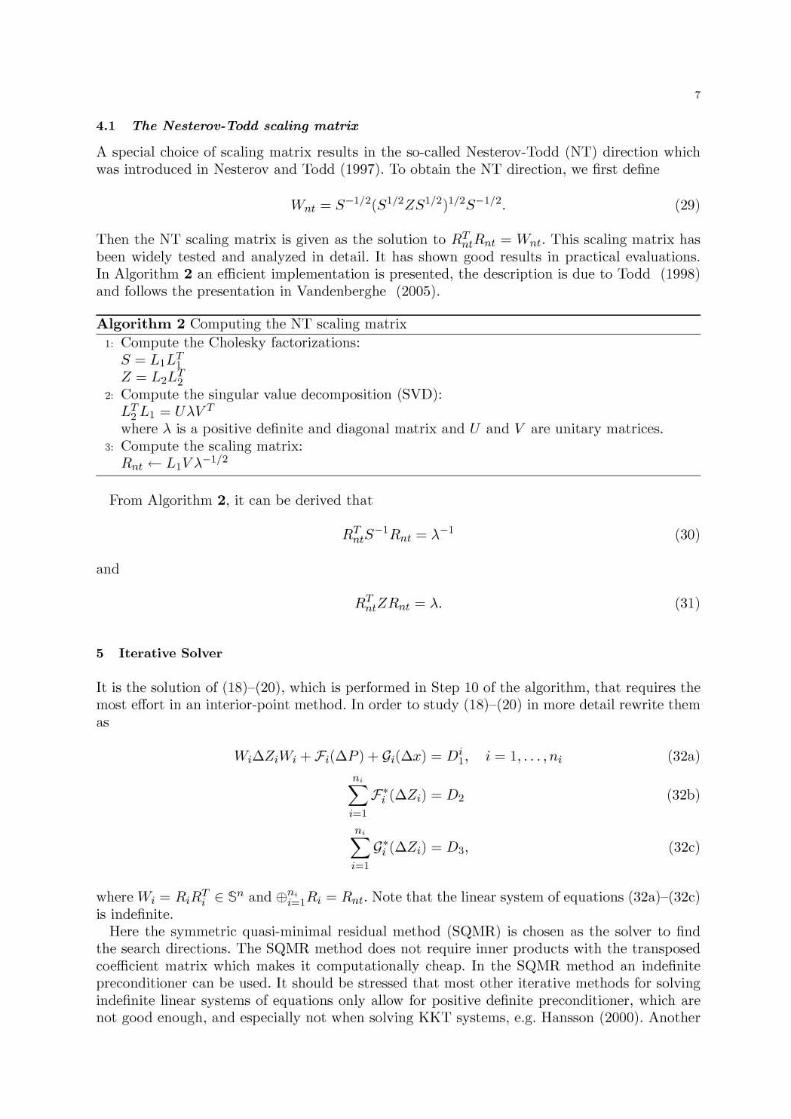
,4.1 The NeJlterov-Todd scaling matrix

A special choice of scaling matrix results ill the so-called Nestcrov-Todd (NT) direction whichwas introduced in Nestcrov and 'lbdd (1997). To obtain the NT direction, we first define

(29)

Theil the NT scaling matrix is given as the solution to rt[t F4.t = IV"t. This scaling matrix hasbeen widely tested and analyzed in detail. It has shown good results in practical evaluations.In Algorithm 2 an efficient implementation is presented, the description is due to 'lbdd (1998)and follows the presentation in Vandenberghe (2005).

Algorithm 2 Computing the NT scaling matrix1: Compute the Cholesky factorizations:

S = L1Lrz= ['Z['2

2' Compute the singular value decomposition (8VD):LfL I = U)..vT

where A is a positive definite and diagonal matrix and U and V are unitary matrices.3: Compute the scaling matrix:

Rnt +- L1VA-1jZ

Prom Algorithm 2, it can be derived that

(30)

and

(31 )

5 Iterative Solver

II is the solution of (18)-(20), which is performed in Step 10 of the fllgorithm, thflt requires themost effort in an interior-point method. In order to study (18)-(20) in morc detail rewrite them~

W;.6..Z;W;+F;(.6..P)+G;(.6..x) = DC i= 1, ... ,11;

!1;

LF;("Z.) ~ D,;=1

".L g;("Z.) ~ D,.;=1

(32fl)

(32b)

(32c)

where W; = R;RT E 5" and EB~~l R; = Rut. Note that the linear system of equations (32a)-(32c)is indefinite.

Here the symmetric quasi-minimal residual method (SQro.1R) is chosen as the solver to findthe searcll directions. The SQl'\'IR method does uot require iuner products with the transposc-'dcoefficieut matrix which makes it computationally cheap. In tile SQ!vIR method au iudefinitepreconditioner cun be used. It should be stressed that most other iterative met.hods for solvingindefinite linear systems of equations only allow for positive definite preconditioner, which arenot good enough, and especially not when solving KKT systems, e.g. Hansson (2000). Another

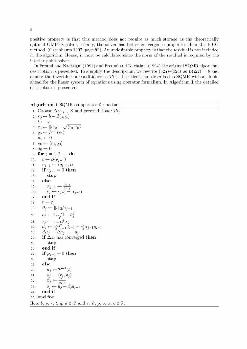
p08itive property is that this method does not require as much storage as the theoreticallyoptimal GMRES solver. Finally, the solver has better convergence properties than the BiCGmethod, (Greenbaum 1997, page 92). An undesirable property is that the residual is not includedin the algorithm. Hence, it must be calculated since the norm of the residual is required by theinterior-point solver.

In F'reund and Nachtigal (1991) and Freund and Nachtigal (1994) the original SQJ'·..IR algorithmdescription is presented, 'lb simplify the description, we rewrite (32a)-(32c) as B(tl.z) = banddenote the invertible preconditioner as P(·). The algorithm described is SQMR without look­ahead for the linear system of equations using operator formalism. In Algorithm 1 the detaileddescription is pre5ellted.

Algorithm 1 SQl"dR on operator formalism

3Z:

24:

27:

23'

t +- rjaj +- Il t I12/7 j_1

Cj+-l/Jl+t9]

7j .- 7j_1 ajCj

dj +- cjt9;_ldj - 1 + cjaj_lqj_1tl.zj +- tl.Zj _ 1+ djif tl.zj has converged then

stopend ifif Pj_1 = 0 then

stopelse

Uj+-p-I(t)Pj +- (Tj,tlj)

/3' +-...£LJ P,_l

;\3: qj +- 11j + /3jqj-1

34: end if35: end for

;11:

25:

I: Choose tl.Z(O) E Z and preconditioner P(·)z: ro +- b- B(z(o))3' f +-ro4' 70 +-lltllz = V(TO,TO)5: (/0 +- p-l(ro)6: ao +- 07: Po +- (ro, qo)8: do'-O9' for j = 1,2, ... do

10' t +- B(qj-tl

11: tij_1 +- (1)_1, f)IZ: if tij_l = 0 then13: stop14: else15' (\"_1 +- PI-'

J "i-l16' Tj +- Tj_1 - OJ_If17: end if18:

19:

28:

"w

21:

"

Hereb,p, T, t,q, dE Z and 7, {), P, u,a, cE lR.

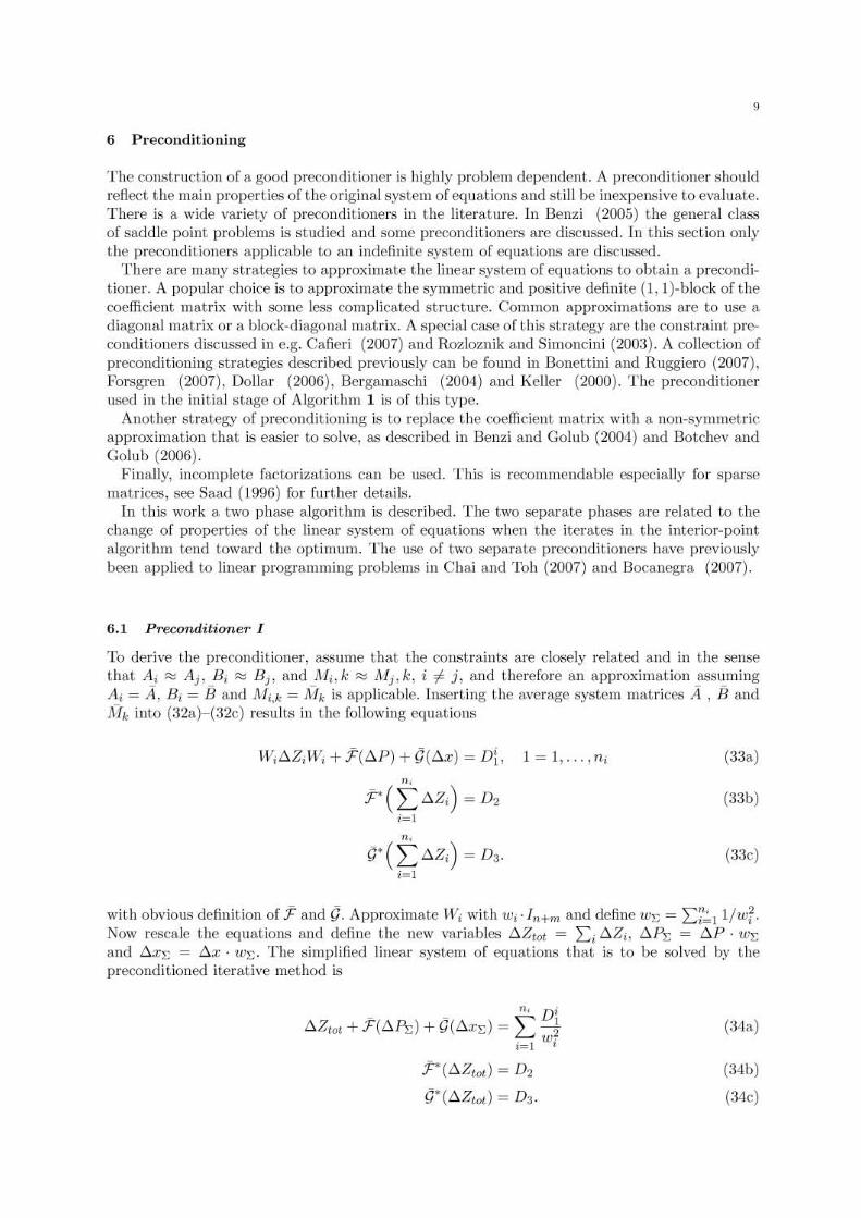
6 Preconditioning

The construction of a good precollditioner is highly problem dependellt. A precollditioller shouldreflect the main properties of the originnl system of equations and still be inexpensive to evaluate.There is a wide variety of preconditioners in the literature. In Bemd (2005) the general c1as.<;of saddle point problems is studied and some preconditioners are discussed. In this section onlythe preconditioners applicable to an indefinite system of equations are discussed.

There are many strategies to approximate the linear system of equations to obtain a precondi­tioner. A popular choice is to approxinlate the synlnletric and positive defiltite (1,1 )-block of thecoefficiellt matrix witll some less complicated structure. CommOll approximations are to use adiagonal matrix or a block-diagonal matrix, A special case of this strategy are the constraint pre­conditioners discussed in e.g. Cafieri (2007) and Rozloznik and Simoncini (2003). A collection ofpreconditioning strategies described previously can be found in Bonettini and Ruggiero (2007),Forsgren (2007), Dollar (2006), Bergamaschi (2004) and Keller (2000). The preconditioner1lSt--'d in the illitial stage of Algorithm 1 is of this type.

Another strategy of preconditiollillg is to replace the coefficient matrix with a lion-symmetricapproximation that is easier to solve, as described in Benzi and Golub (2004) and Botchev andGolub (2006).

Pinally, incomplete factorizations can be used. This is recommendable especially for sparsematrices, see Saad (1996) for further details,

In this work a two phase algorithm is described. The two separate phases are related to thechange of properties of the linear system of equations wilen the iterates ill the interior-poilltalgorithm tend toward the optimum. The lise of two separate preconditioners have previouslybeen applied to linenr programming problems in Cllfli and Toh (2007) and Bocanegra (2007).

6.1 Preconditioner I

To derive the precollditioner, assume that the constraints are dosely related and ill the sensethat Ai "" A j , Bi "" B j , and Mi,k "'" Mj,k, i #- j, and therefore an approximation assumingAi = A, B i = Band Mi,j; = !a~. is applicable. Inserting the average system matrices A , BandRj; into (32a)-(32c) results in the following equations

W;t:.Z;lV; + :F(t:.P) + g(t:.x) = Di, 1 = 1,. ,. ,n;

",p(I>,Z,)=D,

;=1

'I,

a"(L"z,) = D,;=1

(33a)

(33b)

with obvious definition of:F and g. Approximate W; with 'w;·[,,+m and define WE = L7':'1 l/wr.Now rescale the equations and define the new variables t:.Z!ot = L; t:.Z;, t:.Pr; = t:.p. 'WEand t:.:r,;; = t:.x - 'WI> The simplified linear systelll of eqllatiolls that is to be solved by thepreconditioned iterative method is

- - 'I'D;t:.Ztot + :F(t:.Pr;) + 9(t:.XE) = L ----t

1J!,;=1 '

F(t:.Ztot) = D2

g·(t:.Ztotl = D3·

(311a)

(34b)

(34c)

w

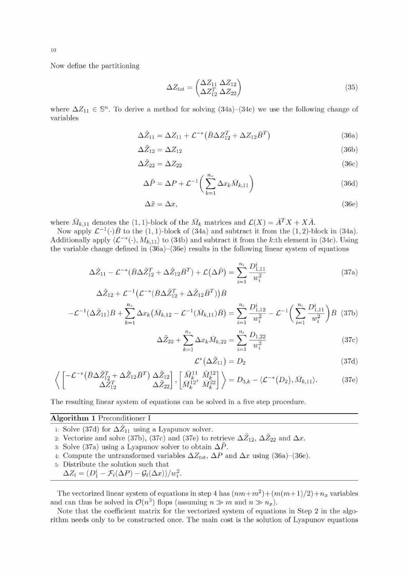
Now define the partitioning

(35)

where ~Zll E $". To derive a met.hod for solving (3'la)-(34c) we lise t.he following change ofvariables

AZl! = AZli + C'(BAZ~; + 6Z12£]")

.:.\Z12 = 6212

AZ22 = AZ:12

6P = 6P + [-1 (I=AXkJfh:.l1)k=l

Ai: = Ax,

(36a)

(36b)

(;loe)

(36d)

(30e)

where A-h,ll denotes the (1, I)-block of the Jfh matrices and [(Xl = ATX + X A.Now apply £.-l(-)B to the (1, I)-block of (34a) and subtract it from the (1,2}-block in (34a).

Additionally apply (l:-*O,Ah"ll) to (34b) and subtract it from the k:th element in (34c). Usingthe variable change dcllned in (36a)-(36e) results ill the following linear system of equations

6211 - c*(Bt.2iz + AZ12 jjT) + C(t.?) = t D~;l1=1 '

A212 + C- 1 (c·(fu::..2iz + 6.Z12 iF)) B

". '" D' ( '" D' )-1 ~ - - -I - - 1,12 _] 1,11--C (AZll)B + L>i.xk(Mk,12 - £. (Mk,lJ)B) = L w~ - C L w~ B

k=1 ,=1' ,=1'

The resulting linear system of equations can be solved in a five step procedure.

Algorithm 1 Preconditioner I

I: Solve (37d) for ~211 miing a Lyapunov solver.2: Vectorize and solve (37b), (37c) and (37e) to retrieve ~ZIZ, ~Zzz and ~x.

3: Solve (37a) using a Lyapunov solver to obtain ~P.

4: Compute the untransformed variables ~Ztot, ~p and ~x using (36a)-(3OO).5: Distribute the solution such that

~Z; = (Dl - :F;(t:.P) - y;(t:.x))jw;'

(37a)

(37b)

(37c)

(37d)

(37e)

The vc-'Ctorized Iillear system of equations in step 4 has (nm+mZ)+ (m(m+ I)/2) +n", variablesand can thus be solved in O(n3) flops (assuming n» m and 11» 11",).

Note that the coefiicient matrix for the vectorized system of equations in Step 2 in the algo­rithm needs only to be constructed once. The main cost is the solution of Lyapunov equations

u

and the solution of the vectorized linear system of equations ill step 4. This can be done at atotal cost of 0(113).

It is noted that the 8SSuniptiollS made to derive the preconditioner is not guarullteed to befulfilled for a geneml problem. it, is obviolls that if these assumption." are violated the convergencespeed will deteriorate for t.he itemtive soker.

6.2 PreconditiQner IT

The illspiratioll to Preconditioller II is found in Gill (1992). [n that work the ullalysis does!lot cOllsider block structure ill the coefficient matrix. Furthermore, the problem is reformulatedto obtain a definite coefficient. matrix since t.he chosen solver requires a definite preconditioner.Here we will construct an indefinite preconditioncr by identifying the constraints that indicatelarge eigenvalues for the scaling matrices and look at the linear system of equations and theblock structure introduced by the constraints.

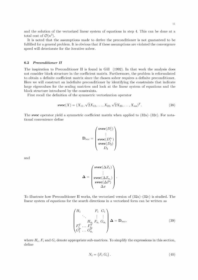
First recall the definition of the symmetric vectorizatioll operator

svec(X) = (X ll , V2X12 , ... , Xn , V2Xn , ... , X",,)T. (38)

The svec operator yield a symmetric coefficient matrix when applied to (32a)-(32c). For not&­tional cOllvenience defille

svec(DJ)

D"·~c = svec(Di")svec(D2 )

03

svec(~Zd

.6. = svec(~Zn,)

svec(~P)

~:r

'lb illustrate how Preconditioner II works, the vectorized version of (32a)-(32c) is studied. Thelillear system of c"quatiolls for the search directions ill a vectorized form can be written as

H,

/ ./ C G ~ = D,.__ ,Il, t"", Il, ~~

P'l pTI· Tor ... Gn ;

(39)

where Hi, Pi and G i denote appropriate sub-matrices. 'Ib simplify the expressiolls in this section,define

N i = (Pi Gi ).

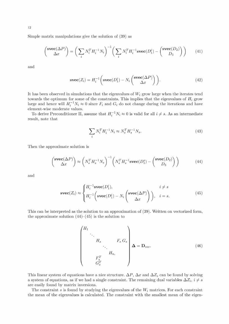
Simple matrix manipulations give the solution of (39) as

and

It has been observed in simulations that the eigenvalues of W; grow large when the iterates tendtowards the optimum for some of the COllstraints. This implies that the eigellvalues of H; growlflrge and hence will H;-IN; ~ 0 since F; flnd G'; do not change during the itemtions and lmveelement-wise llloderate values.

To deriye Prcconditioner II, assullle that Hi lN i ~ 0 is valid for all i =f:. s. As an intermediateresult, note that

Then the approximate solution is

{

H,',v~(DD,

svec(Z;) ~ Hil (sveC(D() _N; (.'lve;:p)) ),i =f:. s

i = s.(45)

This can be interpreted as the solution to an approximation of (39). Written on yectorized form,the approximate solution (44)-(45) is the solution to

("6)

TF,aT,

This lillear system of equations have a nice structure. tJ.P, 6.x and tJ.Z, can be found by solvinga system of equations, as if we had a single COllstraint. The remaining dual variables 6.Zi , i '" S

are easily found by matrix im·ersions.The constraint s is found by studying t.he eigenvalues of t.he W; matrices. For each constraint

the mean of the eigenvalues is calculated. The constraint with the smallest mean of the cigen-

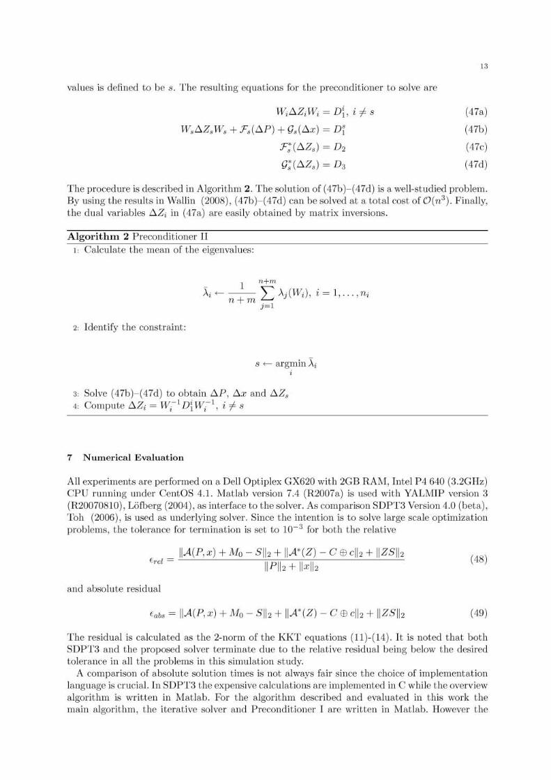
values is defined to bc s. The resulting equations for the preconditioner to solve are

W;IlZ,IV; = DL i # s

W~IlZ~W$ + F~(IlP) + 9Allx) = DfF;(IlZ.) = D2

g;(IlZ~) = D3

(47a)

(47b)

(47c)

(47d)

The procedure is describc-'d in AIgOritlllll 2. 'rhe solutio!l of (47b)-(47d) is a well-studied problem.By using the results in Wfl.llin (2008), (47b)-(47d) CRn besoh-ed at a total cost ofO(n3). Finfl.lly,the dual variables llZ; in (47a) are easily obtained by matrix inversions.

Algorithm 2 PreCOllditioner III: Calculate the mean of the eigellvalues:

_ I n+m

-\ +- -- '" Aj(Wil, i = I, ... ,n,n+m~

j=1

2: Identify the constraint:

s +- argmin Xi;

3: Solve (47b)-(47d) to obtain llP, llx and llZ$4: Compute llZi = lV;-l D( lV;-I, i # s

7 Numerical Evaluation

All experiments are performed 011 a Dell Optiplex GX620 witll 2GB RA1'I'I, Intel P4 640 (3.2GHz)CPU running under CentOS 4.1. 1'1'latiab version 7.4 (R2007a) is used with YALi\UP \'ersion 3(R20070810), LOfuerg (2004), as interface to the solver. A$ comparison SDPT3 Version 4.0 (beta),'lbh (2006), is used as underlying solver. Since the intention is to solye large scale optimizationproblcms, the tolerance for termination is set to 10-3 for both the relativc

and absolute residual

IIAIP, xl + AI, - 511, + IIA'IZ) - C Ell ,Ib + IIZSlbIWlld II xll,

(48)

(49)

The residual is calculated as thc 2-norm of the KKT equations (11)-(14). It is noted that bothSDP'l'3 and the proposed solver terminate due to the relative residual being below the desiredtolerance ill all the problems in this shnulatioll study.

A comparison of absolute solution times is not always fair since the choice of illlplementatiolllfl.nguage is crucifl.1. In SDPT3 the expensive calculations fl.re implemented in C while the overviewalgorithm is written in !vlatlab. For the algorithm described and eVfl.luated in this work themain algorithm, the iterative solvcr and Preconditioncr I arc writtcn in r-.htlab. Howcvcr the

construction of the coefficient matrix in Preconditioner II is implemented in C and that is theoperation that requires the most computational effort. Obviously an implementation in C of allsul>-steps would improve the described solver. The similarity in the level of implemelltation in Cmakes a comparison in absolute computational time applicable. At least is the proposed solvernot in favour in such a comparison.

The parameters in the algorithm are set to ,.., = 0.01, O"ma", = 0.9, O"",i" = 0.01, r/ = 10-6,X = 0.9, ( = 10-8 and f3 = 107. f3li"', where f31im = max(IIA(P, xl + Alo- Sllz, IIA*(Z) - C$cllz).The choice of parameter values are based on knowledge obtained during the development of thealgorithm and through continuous evaluation. Note that the choice of 0"",= is not within therange of values in the COllvergence proof givell in the appelldix. However, the choice is motivatedby as good convergence as if 0"",,,,,, E (0"",;,,,0.51. This can be motivated by the fact that valuesclose to zero and one correspond to predictor and corrector steps respecth·ely.

Switching betwccn the preconditioners is made after ten iterations. This is equivalent to fivepredictor-corrector steps. A more elaborate switching technique could improve the convergencebut for practical use, the result is satisfactory.

The only ill formation that PrecOllditiOller [1 is givell, is if the active constraillt has changed.This information is obtained from the main algorithm.

10 obtain the solution times, the i\'1atlab command cputime is lISed. Input to the soh-ers arethe system matrices, so any existing preprocessing of the problem is included in the totnl solutiontime.

In order to monitor the progress of the algorithm the residual for the search directions iscalculated in each iteration in the iterative solver. '10 obtain further improvement in practice,one could use the in SQMR for free available bi-colljugate gradient (BCG) residual. Howeverthis results in that the exact residual is not kllown and hence the convergence might be afk"Cted.

Initialization

For comparable results, the initiali,.;ation scheme givell in 'Ioh (2006) is used for the dualvariables,

((n+ln)(l+ICJ.,I))

Zi=max 1O,vn+ m, -.!uax 11\1 II I,,+m,k_I, ... ,,,, 1 + j l.k Z

where II . liz denotes the Frobenius norm of a matrix. The slack variables arc choscn as Si = Ziwhile the primal variables are initialized us P = I" and x = 0,

Examples

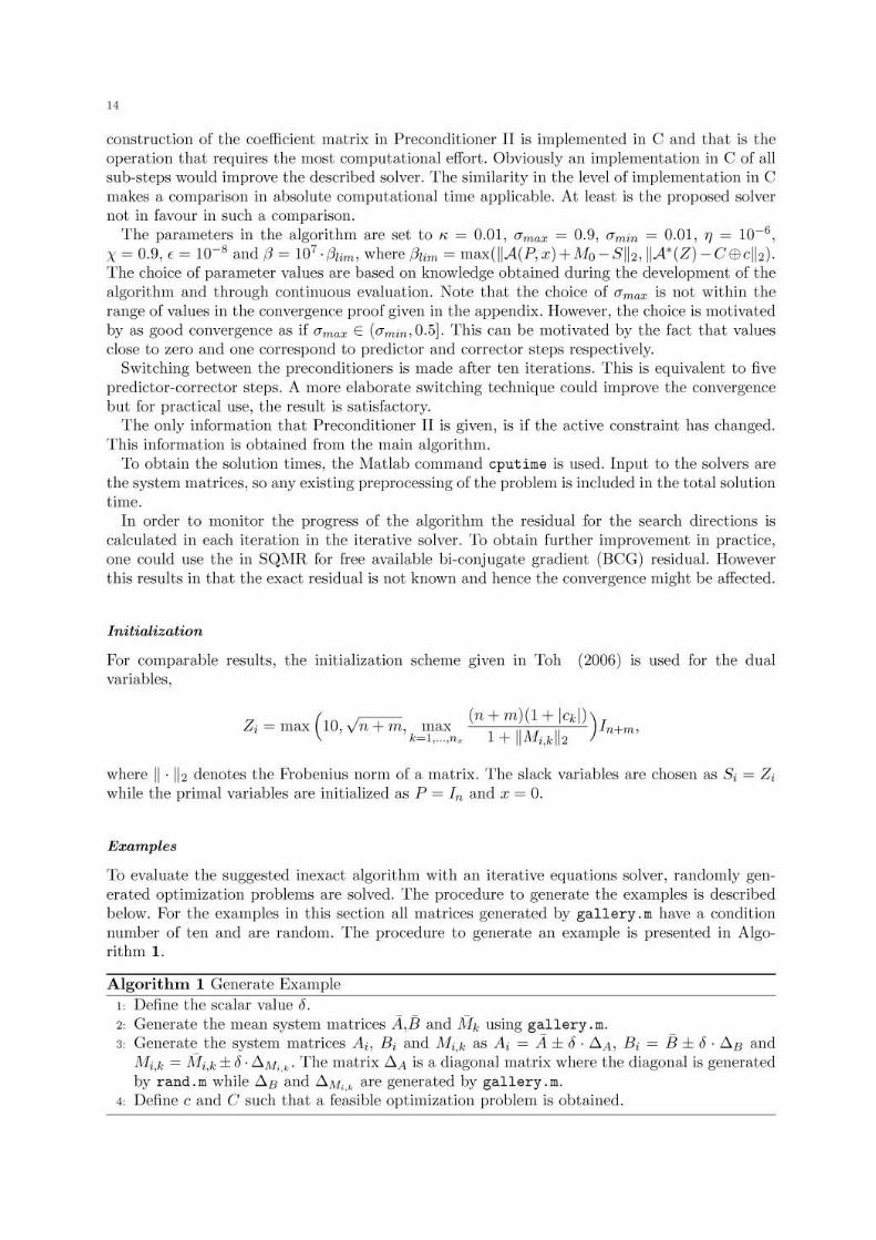
'10 evaluate the suggested inexact algorithm with an iterative equations solver, randomly gen­erated optimization problems are solved, The procedure to generate the examples is describedbelow. For the examples in this section all matrices gellerated by gallery.m have a conditiOllnumber of ten and are random. The procedure to gellerate an example is prcscllted in Algo­rithm 1.

Algorithm 1 Generate ExampleI; Define the scalar value 6.z: Generate the mean system matrices it,ll and A-Ik using gallery.m.3: Generate the system matrices Ai, B i and Mi,k as Ai = .4 ± 6· toA, B i = B ± 6· toB and

Mi•k = Ini,k ± 6 - toM;,., The matrix toA is a diagollal matrix where the diagonal is generatedby rand.m while to8 and toM;. are generated by gallery.m.

4: Define c and C such that a feasible optimization problem is obtained.

Results

'lb make an exhaustive investigation, different problem parameters have been invcstigated:

n E {10, 16,25,35,50, 75, 100,130, 165}

mE {I,3,7}

n; E {2,5}

J E {0.01,O.02,0.05}

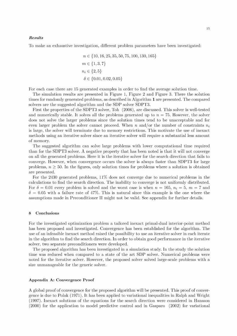
For each case there are 15 generated examples in order to find the average solution time.The simulatioll results are presented ill Figure I, Figure 2 and Figure 3. There the solutioll

times for ralldomly generated problelllS, as described in Algorithm 1 are presented. The comparedsolvers are the suggested algorithm and the SOP solver SOPTa,

First the propertics of the SDPT3 solver, Ibh (2006), are discussed. This solver is \\"ell-tcstedand numerically stable. It solvcs all the problems generated up to n = 75. However, the solverdoes not solve the larger problems since the solution timcs tend to be unacceptable and foreven larger problem the solver cannot proceed. \Vhen n and/or the number of constraints n;is large, the solver will terminate due to memory restrictiolls. This motivate the use of inexactmethods using an iterative solver since an iterative solver will require a sl1bst.antialless amountof memory.

The suggcsted algorithm can solve large problems with lo\\"er computational time requiredthan for the SDP'l'3 solver. A negative property that has bccn noted is that it will not convergeon all the generated problems. Here it is the iterative solver for the search direction that fails toconverge. However, when convergence occurs the solver is always faster than SOPT3 for largeproblems, n ~ 50. In the figures, only solution times for problems where a solution is obtainedare presented.

For t.he 24;10 generated problems, 11% does not converge due to numerical problems in thecalculations to find the search direction. The inability to converge is not uniformly distributed.For J = 0.01 every problem is solved and the worst case is when n = 165, n; = 5, In = 7 andJ = 0,05 with a failure rate of 47%. This is natural since this example is the one where theassumptiolls made in PreconditiOller II might 1l0t be valid. See appendix for furtller details.

8 Conclusiolls

For the investigated optimization problem a tailored inexact primal-dual interior-point methodhas been proposed and investigated. Convergence has bccn established for the algorithm. Theuse of an infeasible inexact method raised the possibility to use an iterative solver in each iteratein the algorithm to find the search direction, In order to obtain good performance in the iterativesolver, t\\"o separate preconditioners were developed.

The proposed algorithm has been investigated in a simulation study. In the study the solutiolltime was reduced when compared to a state of t.he art SOP soh-cr. Numerical problems werenoted for the iterative solver. However, the proposed solver solved large-scale problems with asize unmanageable for the generic solver.

Appendix A: Convergence Proof

A global proof of convergence for the proposed algorithm will be presented. This proof of conver­gence is due to Polak (1971). It has been applied to variational inequalities in Ralph and Wright(1997). Inexact solutions of the equat.ions for the senrch direct.ion were considered in Hansson(2000) for the application to model predictive control and in Gasparo (2002) for variational

"1"2,m- ,

00' rr==c==",-'--'--'---'----,1-'"""'1- - -$DPT3

00'

.,, .

i! ;/1'

",:,,,,,

00'

"I"S,m-,

00' rr==c==",,'--'--'---'----,1-'"'''"1- - -$DPT3,

!; ,,,,,,,,,

--00'

00'

SiZe of A malnx00'

00' 00'

,,,

"I'" 5, m "'3

00' ir=='7.'::';o;,--"---,1- '""'" I "---SDPT3 I

I . ..,, ; ";, ­,,,,,

S'ze 01 A mallix00'

!FlO'

"I'" 2, m "'3

00' 1'=='7.':::;0;---'----,"1- ,""~octI '- - -SDPT3

;,,,,,,,,,00' 1----.,-,;.--

"00'

S'ze of A malnx

. ,,,,',',,,

,,

"I"S,m-7

00' ir=='7.':::;o;'---:---7'11-'""'"1- - -SOPTJ

00'

!FlO' 1---:",,

,,,,,

,,,

00'

"1"2,m-7

00' ir=='7.':::;o;----:---"1-'"""'1- - - SDPT3

!FlO'

00'

00' 00' 00' 00'Size of A matrix Size 01 A matrix

Figure 1. Solution tin"", for randomly generated problc1IIlI. The sugg""too inexact primal-dual interior-point method iscompare<! to the SDPT3 soh..". [n the example; 6 = 0.01. For ca.ch plot the solubon time is plotted as a function ofsr'tcrnorder fl.

inequalities. The convergence result is that either the sequence gCllerated by the algorithm ter­minates at a soluUon to the Kflrush-Kuhn-Tucker conditions in fl. finite llumber of iterations, orall limit points, if any exist, flre solutions to the Karush-Kuhn-Tucker conditions. Here t.he proofis cxtcndcd to the casc of scmidefinite programming.

"1- 2,m-! "I-S,m-,

,,' ,,'1-'"""'1 I-'","ctl ,

- - -SDPT3 - - -SDPT3~., ..

,,' "i ,,' ,, ,, ,.~ , ~ ,~

,.! ", ,,,' , " ,,' ,, ,, ,,

,,' , ,,',,-,,' ,,' ,,' ,,'

$geo1A malri. $geo1 A malri.

"1- 2,m-3 "I- S,m-3

,,' ,,'1-'"""'1 I-'""'ctl ,

- - -SDPT3 - - -SDPT3 ,,,' , ,,' ,, ,, ,

~ , ~,

!-- 'r

!,, ,

" ,,' ,." ,,' ,, , ,,

,,,' " ,,' "

,,' ,,' ,,' ,,'Sge of A matrix Sge of A matrix

".-2,m-7 ".-S,m-7

,,' , ,,' ,

1-"'""'"1 1-'",",,,ct1 .: ,- - -SDPT3 - - -SDPT3

"", .. ,,,' , ,,' ,

!; , ;! ,~

,~

,, ,!

,!

" ,,' " ,,', ,, ,, , ,,,,,' -- ,,'" ,

,,' ,,' ,,' ,,'Sge 01 A main. Sgeo1 A malO.

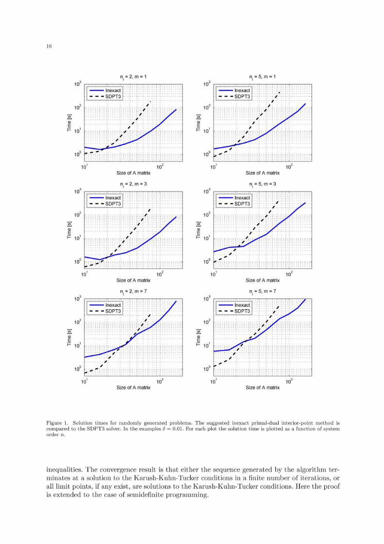
Figure 2, Solution timet< [or randomly generate<! problem". The "ugge,te<! inexact primal_dual interior_point method iscompare<! to the SDPT3 ",,"..,r. In the exampl"" 6 = 0.02. For each plot the ""Iu<ion time i" plotte<! as .. function of "rstemorder n,

A.I Convergence of Inexact Interior-Point Method

In order to prove cOllvergellce some preliminary results are presented in the following lemmas.First we define the set n+ as

11+ = {z E 1115;- O,Z ;-O}. (A I)

n, - 2, m- , n,-5,m-j

00'

1-""'"""'1" 00'

1-"'"""'1 .- - -SDPT3 - - -SDPT3 ",

00',

00' , i;, ,~

,~

,, ,! :, , ! ,, ,F 00' " F 00' ,, ,, ,,

00' 00'

00' 00' 00' 00'SiZe of A mallix Size of A mallix

n, - 2, m_' n, - 5, m_'00' 00'

1-'"·''''1 1-'"·''''1 :,- - -SDPT3 - - -SDPT3 ,00'

,00'

,, ,

"

,, ,~ , ~ ,~

,~

,, ,00' , 00' ,,, ,,-- ,00' 00'

,,

00' 00' 00' 00'SiZe of A mallix Size of A mallix

n, _ 2, m_ , n, _ 5, m_ ,00' 00'

1-'"·-1 1-'"·-1 :'- - - SDPT3 - - -SDPT3 ,'r . ,

00',

00' ,, " ' "~

,~

,,! ! ,F 00' F 00'

,, ,, ,, ----,

00' , , , 00' , , ,00' 00' 00' 00'

Size of A matrix Size of A matrix

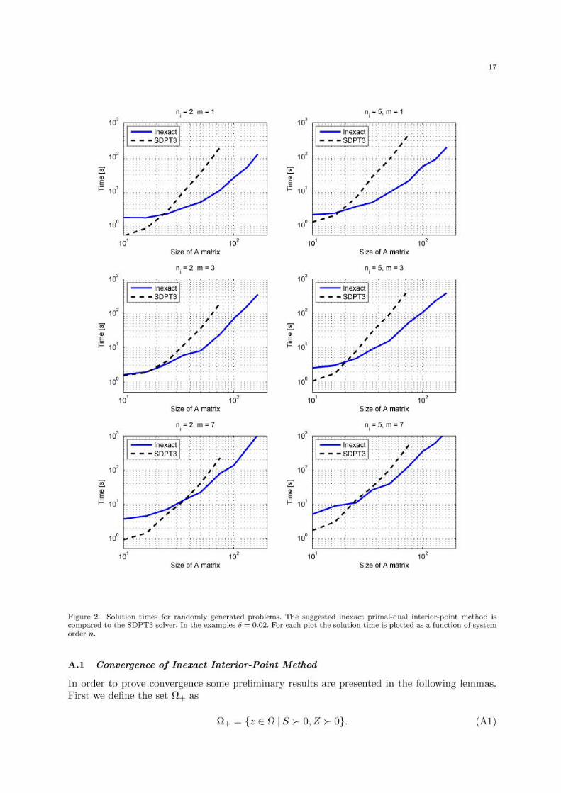
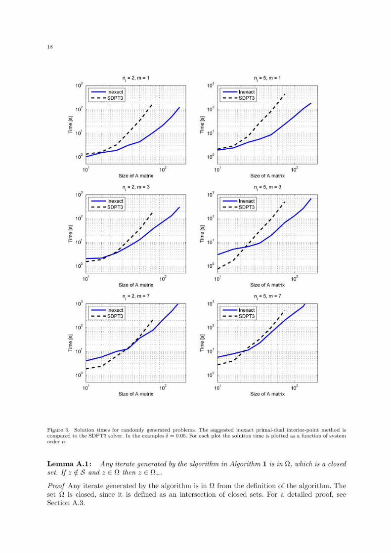
Figure 3. Solution tiJI>e!l for randomly genera.ted problems. The sugg.,,;ted inexa.et prima.l-dual interior-point method iscompared to the SDP'/'3 soh·cr. In the cxample; 6 = 0.05. For c""h plot the solution time is plotted M" function of systemorder" .

Lenm-rn A.I: Any itemte generated by the a(qorithm in Algorithm 1 is in n, which is (I closedset./fzif-S andzEIl lhenzEl!+.

Proof Any iterate generated by t.he algorithm is in 11 from t.he definition of t.he algorithm. Theset. 11 is dosed, since it is defined a.<; an intersection of dosed sets. For a detailed proof, seeScct.ion A.3.

The rest of the proof follows by contradiction, Assume that z rt s, zEn and z rt n+. Nowstudy the two cases v = 0 and v > 0 separately, Note that v '2: 0 by definition,

First assume that v = O. Since v = 0 and zEn it follows that A:dz) = 0, IIKp(z)lIz = 0 andIIKd(z)llz = O. This implies that Kp(s) = 0 flnd Kd(s) = O. Note that zEn also implies thatZ t 0 and S t O. Combing these concl1L~ions gives that z E 5, which is a contradiction.

Noll' assume that v > O. Since v > 0 and zEn it follows that K,otz) = 1t(ZS) >- O. 'lbcomplete the proof two inequalities are needed. First note that det(1t(ZS)) > O. To find thesecond inequality the Ostrowski-Taussky inequality, see page 56 in Lutkepohl (1996),

x+xT

det ( 2 ) ~ Idet(X)I,

is applied to the symmetry trallsfonnation. This gives

det(1t(ZS)) ~ Idet(R- 1ZSR)I = Idet(Zll·1 det(S)1 = det(Z)· det(S),

where the last equality follows from zEn. Combining the two inc"'qualities gives

0< det(1t(ZS)) ~ det(Z)· det(S).

(A2)

(A3)

Since t.he determinflnt is the product of all eigenvfllues and zEn, (A;1) shows that the eigenvflluesare nonzero flnd therefore Z >- 0 and S >- 0, This implies that. Z E n+, which is fl cont.mdiction.o

The linear system of equat.ions in (18)-(20) for the step direct.ion is now rewrit.t.en flS

&vec(K:(z))&vec(z) vec(t:.z) = vec(r). (M)

Note that the vectori<:ation is only used for the theoretical proof of convergence. In practicesolving the equations is preferably made with a solver based on the operator formalism.

Lemma A.2: Assume that A has full rank. Let i E n+, and let (0 E (0,1). Then there existscalars &> 0 and 6: E (0, II SllCh that if

11

8vec(K:(,)) II '&vec(z) vec(t:.z) - vec(r) 2 ~ 'ia{3v,

iJvec(I(,(,))Clvec(z) vec(t:.z) - vec(rc) = 0,

and if the algorilhm lakes a step from any poillt in

(A5)

(AB)

(A 7)

othen the calculated step lenglh a will satisfy a '2: 6:.

P1"()()f See Section A.2.

Now the global convergence proof is presented.

Theorem A.3: Assume that A has full rank. Then for the iterates genemted by the interior­point al.qorithm either

z(j) E 5 for some finite j.- all limit points of fz{j}} belongs to 5.

Remark Al: Note that nothing is said about the existence of a limit point. It is only statedthat if a convergent subsequence exists, then its limit point is in 5. A sufficient condition for theexistence of ulimit point is that {z(j)} is uniformly bounded, Polak (1971).

pT(l()f Suppose that the sequence {z(j)} is infinite and it has a subsequence wldch converges to£ rt 5, Denote t.he corresponding subsequence {j;} with K.. Then for all 8' > 0, there exist a ksuch that. for j 2': k and j E K. it holds t.hat.

lAS)

Since £ rt 5 it holds by Lemma A.I that £ E n+ and hence from Lemma A.2 and (8) that thereexist a 3 > 0 and ii E (0, I] such that for all z(j), j 2': k such that Ilz(jl - £112:::: 6 it holds that

Now take <5' = 6, Then for two consecutive points z(jl' z(j+i) of the subsequence with j :::: k andj E K. it holds that

V(j+i) - v(j) = (V(j+i) - vU+i-l)) + (I/(i+i-l) - V(j+i_2) + ... )+ (I/(j+l) - v{j))

, "< 1/(j+1) - v(jl :::: -0:"'( I - (Tmax)<5 < O.lAg)

Since K. is infinite it holds that {/J(jl}iE"': diverges to -00. The assumption £ E n+ gives thatf) > 0, whicll is a contradiction. 0

10 simplify the proof of Lemma A,2, two preliminary lemmas are presented,

Lemma A.4: Assume A E S~· is symmetdc. If IIAI12:::: 0, then

Pmof Denote the i:th largest eigenvalue of a matrix A with Ai(A). Then the norm fulfills

,II All; ~ L AC(A),

i=l

sec (Boyd and Vandenberghe 2004, p. 647). Then

IA 10)

IA II)

,IIAI12 :::: a ¢9 L A?(A)::; a2 => A?(A)::; a2 => IAi(A)1 ::; a ¢9 -a::; Amin(A)::; Ai(A) :::: A",ax(A)::; a

;=1(AI2)

and hence

IA13)

oLemma A.5: Assume z E 6 as defined in (AJ). Then Z >- Z - 61".(tl+",} and S ~ 5­61";(,,+,,,).

pT(l()f We have liz - i11 2 ::; J. Hence liz - ill~:::: 62 and

'2 "22'2liS - SII, + liZ - ZII, + Ilx - ill, ~, . IA 14)

Therefore liS -Sll~ ~ 32 and liZ - Zll~ ~ 62. Hence by Lemma A.4 above -6/11 ;(I1+m) ~ S-S ~

61,,«,,+m) and -61".{,,+m) ':':: Z - 2 ':':: 61,,«,,+m). 0

A.2 Proof of Lemma A.2

Here a proof of Lemma A.2 is presented. What is needed to show is that there exist an 0 suchthat 0 :::: it > °so that z(o) = z + ot.z E n and that

/1(0) ~ (1- 01,;(1- 0"))/1.

First a property for symmetric matrices is stated for later use in the proof.

A:: B, C:: D => {A,C}:::: (B,D),

where A, B, C, D E S't-, page 44, Property (18) in Liitkepohl (1996).Define

(AI5)

(AI6)

(A 17)

Notice that z E B by Lemma A.5 implies that S ~ S- 31",("+,,,) and Z ~ Z - 31",("+,,,). Thenit holds that

(Z,S)v~

11;(n+m)(2 - 31,,«,,+m), S- 31".("+,,,»)

:::: ::::n;(n + m)

(3 I",(n+m), 31".{,,+m»)n;(n+m)

=32 >0, (A 18)

where the first inequality follows from (AI6) flnd what was mentioned above. The second in­equality is due to (AI7) and (AW). Similarly as in the proof of Lemma A.1 it also holds thatZ,S >- 0.

Now since A has full rank it follows by Lemma 3.1 that (8vec(K:(z))/&vec(z)) is invertible inan open set containing B. Furthermore, it is dear that (&vec(K:(z)) /&vec(z)) is a continuousfunction of z, and that r is a continuous functiOH of z and 0". Therefore, for all z E B, 0" E(o-m;n, 1/21, it holds that t.he solution t.zo of

8vec(K:(z))&vec(z) vec(t.zo) = vec(r), (A 19)

satisfies lIt.zoll z ~ Co for a constant Co > O. Introduce 05t.z = t.z - t.zo. Then from the boundon the residual in the assumptions of this lemma it follows that

(A20)

is bOllllded. Hence there nlust be a constallt 05C > 0 such that 1105t.zllz ~ 05C. Let C = Co +05C >O. It now holds that IIt.zll:.! ~ C for all z E B, 0" E (o-m;n, 1/2]. Notice that it also holds thatIIt.Zllz ~ C aHd IIt.Sllz ':':: C. Define &(1) = 6/2C. TheH for all 0 E (0,6:(1)1 it holds that

Z(o) = Z + ot.Z ~ t - 3'n,(n+",) + ut.Z ~

, , J261";(11+,,,) - 6I";(I1+m} - 2/";(n+,,,) >- 0,

(A21 )

where the first inequality follows by Lemma A.5 and z E B, and where the second inequalityfollows from (A17). The proof for 5(0:) ~ 0 is analogous. Hence is is possible to take a positivestep without violating the constraint 5(0:) ~ 0, Z(o:) ~ O.

Now we prove that

Kc(z) = H(Z(0)5(a)) t: 'Iv(o)/",(,,+mj

for some positive 0:. This follows from two inequalities that utilizes the fact that

avec(Kc(z))" () .dz-vec(rc)=O¢}vvec z

H(6.Z5 + Z6.5) + H(Z5) - o-vl",("+,,,) = 0

(A22)

(A23)

and the fact that the previous iterate z is in the set fl. Note that H(·) is a linear operator. Hence

H(Z(0:)5(0)) = H(Z5 + 0(.6.Z5 + Z.6.5) + 02.6.Z6.5)

= (1 - 0)H(Z5) + 0(H(Z5) + H(.6.Z5 + Z6.5)) + a 2H(6.Z.6.5)

t (1 - o)rwl",("+,,,j + oo-v1",("+,,,) + a 2H(.6.Z6.5)

t ([(1 - 0)'1 +ao-)v - a21..\~;T\I)/",("+,,,j,

(A24)

where ..\~;" = min; ..\;(H(.6.Z6.5)). Note that ..\~;" is bounded. 'Ib show this we note that ineach iterate in the algorithm Z and 5 arc bounded and hence is R bounded since it its calculatedfrom Z and 5. Hence H(6.Z.6.5) is bounded since II6.ZI12 < C and 116.5112 < C.

Moreover

n;(n+m)v(o:) = (Z(o:),S(a)) = (H(Z(a)S(a)),I"dn+m))

= ((1- a)H(ZS) + o:o-vln,{n+",} + cr'U(.6.Z6.S), In,("+,,,j)

= (1 - 0: )(Z, 5) + n;(n + m)ao-v + 0:2 (.6.Z, 6.5)

:::; (1- o:)n;(n + m)v + n;(n + m)o:o-v +a 2C 2.

(A25)

The last inequality follows from (.6.Z,6.5):::; II.6.ZII:;1I1.6.5112:::; C 2 . Rewriting (A25) gives that

(o'C' )

rw(a)$ (l-o:+o:o-)v+ ( ) 'I·n; n+m

Clearly

implies (A22), which (assuming that a > 0) is fulfilled if

0-1.'(1 - 'I)a< _ Il. .

- C2r,/n,(n + m) + P,,,,;,,I

(A26)

(A27)

(A28)

Recflll that 0- 2': <Tm;n > 0, 1/ < 11max < I by assumpt.ion and that. 0 < 62 $ v by (A 18). Hence

with

(A22) is satisfied for all 0 E (0,&(2)1.We now show that

1'/.'(0:)1>1;(>1+"') t 1i(Z(0:)5(0:)).

First notc that l' ;::: n; (n + m). Then

(" ) L'.(H(Z(aIS(a))) ~ 'm=(HIZla)S(a))) '*H; n+m .,

(1' ) L)";(1i(Z(0)5(0)))1" (,,+m) ~ '>'maz(1i(Z(0)5(o)))1,,;(,,+m) <=}n; n+m . .,

n;(n:.. m) Tr(1i(Z(o)5(0))) 1";(>1+mj ~ '>'max (1i(Z(o )5(0:))) 1";(>1+mj,

(A29)

(A30)

where the first expression is fulfilled by definiti01I. The second c"quivulellce follows fronl a propertyof the trace of a nlatrix, see page 41 ill Liitkepohl (1996). FrOl1l the definiti01I of dualilty Illeasurein (8) it now follows that (A30) holds.

Now wc provc that (AI5) is satisfied. Let

Then for all 0: E [0, &l3}] it holds that

0 20 2 :s; a"ni(n + m)( 1 - ",)62/2

:s; on;(n + m)(l - 1i)/.'/2

:S;oni(n+m)(I-",j(I-a)v,

(A31)

(A32)

where the second inequality follows from (A18) and the third inequality follows from the as­sumption Q:S; 1/2. This inequality together with (A25) implies that

0 20 2

/.'(0) :s; ((1 - 0) + oa)/.' + -2-

:s; ((1- 0:) + oa)/.' + 0(1 - 1i)(1 - a)

~ (1 - a.(1 - al),

whcrc thc second inequality is due to Q < 1/2 and hcnce (AI5) is satisfied.It now remains to prove that

IIK,I*I)II, ~ ~"(al

IIK,I,(al)lb ~ ~"(al,

(A3'la)

(A;3'lb)

Since thc proofs arc similar, it will only be proven that (A34a) holds true. Use Taylor's thcorcm

to write

&vee(K (z))vee(Kp(z(a))) = vee(Kp(z)) + a ? r) vee(llz) + oR

(vee z

where

R = t (&vec(K,,(z(Oa))) _ ovec(Kp(z))) . vec(llz)<iO.io ovec(z) ovec(z)

Using Ilz = Ilzo +6Ilz and the fact that

8vec(Kp(z))o () vec(llzo) = -vec(K,,(z)),uvec z

it follows that

(A35)

&vec(Kp(z))vee(Kp(z(a))) = (I - a)vec(Kp(z)) + a &vec(z) vec(6Ilz) + aR. (A36)

Furthernlore

IIRllz:5 max II&vec(Kp(z(Oa))) - &vec(Kp(z)) II ·llvec(llz)11z. (A37)Oe(o,l) &vec(z) Glvec(z) z

Since IIIlzllz :5 C and since &vec(Kp(z))/&vec(z) is continuous, there exists an 0(4) > 0 suchthat for a E (0,0(4)], (E (0, I) and z E B it holds that

1-,IIRllz < -,-u{3v,

Using the fact that IIKp(z)112 :5 {3v, it now follows that

for all a E [0,0(4}]. By reducing 0,(4), if necessary, it follows that

aC2 < ~ni(n + m)v,

for all a E [0,0(4)] . Similar to (A25), but bounding belo\\' instead, it holds that

(A38)

(A39)

(A40)

( n'c' ) a (nO'IIKp (z(a))1I2:5 {3 v(a)-ouv+ ( ) +a-f3v = {3v(a)-a{3 uv- ( )ni n+m 2 nj n+m

Hence

av)2 :5 {3v(a),

(A42)where the last inequality follows from (A40). The proof for Kd(z(a)) :5 {3v(a) is done analogously,which gi\"cs an 0(5) > O.

REFERENCES

A.3 Pruof of Closed Set

Here the proof of that the set n defined in (27) defines a closed set is presented.

Definition A.6: Let X and Y denote two metric spaces and define the mapping j; X ----> Y,Let C';;; Y, Then the inverse imagerl(C) ofC is the set {x 1J(x) E C, xE X}.

Lemma A.7: A mapping oj a metric space X into a metric space Y is contimwus ij and onlyif rl(C) is closed in X JOT every closed set C.;;; Y.

Proof See page 81 in Rudin (1970). 0

Lemma A.S: 'rhe set {z IIIK:p (z)112 ::; fill, z E Z} is a closed set.

P1"Oof Consider the mapping K:p(z) : Z ---+ S" and the set C = {C IIICllz ::; fill, C E S"} thatis closed since the norm defines a closed set. This follows from that we have C = J- I ([0, ,Bv]),where J(-) = II· liz· Now the claim follows by Lemma A.7. To see tlds lIote that the mappillgK:p(z) is continuous. Then the inverse image {zlK:,,(z) E C, z E Z} = {zlllK:p (z)1I2::; (:JII, z E Z}is a closed set. 0

Lemma A.9: 'rhe set {z 11IK:(J(z)llz::; ,Bv, z E Z} is a closed set.

P1"Oof Analogous with the proof of Lemma A.8. oLemma A.tO: The set {z I,vl,,;(,,+m) ~ H(ZS)::: 1WI",(,,+m), Z E Z} is a closed set,

Proof Define the mapping h(z) = H(ZS); Z ---t S" and the set Cl = {CdCl :::/Wl,,;(n+m), C l ES"} that is closed, page 43 in Boyd and Vandenberghe (20t)4). Since the mapping is continuousthe inverse image {z 1H(ZS) ::: 1/111",("+,,,), z E Z} is a closed set. Now defIne the set Cz ={CzICz :::; 1/111";(,,+,,,), Cz E S"}. Using continuity again gives that {zIH(ZS) :::; ,vl".{,,+m), Z EZ} is a closed set. Since the intersection of closed sets is a closed set, Theorem 2.24 in Rudin(1976), {z 1~(/II,,;(,,+m) ~ 1i(ZS)::: J/v1n,{,,+m), Z E Z} is a closed set. 0

Lemma A.ll: The set n is a closed set.

Proof Note that (Z,p) is a metric space with distance p(l1,ti) = 1111-1)112. Hence is Z a closedset. Lemmas A.8, A.9 and A.IO gh'es that each constraint in 11 defmes a closed set. Since theintersection of closed sets is a closed set, Theorem 2.24 in Rudin (1976), shows that 11 is a closedset. 0

Referellces

Boyd, S., Laurent, E.G., Feron, E., and Balakrishnan, V., Linear Matrix inequalities in Systemand Control Theory, SIAM (1994).

Gahinet, P., Apkarian, P., and Cbilali, M. (1996), UParameter-Dependent Lyapunov Functionsfor Real Parametric Uncertainty," IEEE Transactions on Automatic Cont1"01, 41(3), 436­442.

Wallg, F., and Balakrisllllan, V. (2002), ulmproved stability analysis and gaill-scheduled COll­troller synthesis for parameter-dependent systems," Alltomatic Control, IBBB Transae/io/ISon, '17(5), 720-734.

LOlberg, J. (2004), "YALMrp : A 'lbolbox for ~'1odcling and Optimization in !'.Iatlab," in Pro­ceedings of the CACSD Confe7Y311ce, Taipei, Taiwan.

'lbh, K.C., 'lbdd, M.J., and Tiltiincil, RH. (2006), "On the implementation and usage of SDPT3- a !\'Iatlab software puckuge for sentideflnite-quadratic-linear programming, version 4.0,"

Benson, S..1., and Yinyu, Y. (2005), "DSDP5; Software For Semideflnile Programming," Tech­nical report, I\'lathematics and Computer Science Division, Argonne National Laboratory,Argonne, IL.

REFERENCES

Sturm, J.P., UUsing ScDuMi 1.02, a matlab toolbox for optimization over symmetric cones,"(W01).

P61ik, 1., uAddendum to the SeDul'l'li user guide, version 1.1," (2005).Chai, J .S., and Toh, K.C. (2007), "Preconditioning and iterative solution of symmetric indefinite

linear systems flrising from interior point methods for linear programming," ComputationalOptimization and Applications, 36(2-3), 221-247.

Bonettini, S., and Ruggiero, V. (2007), uSome iterativc methods for the solution of a symmctricindefinite KKT system," Computational Optimization and Applications, 38(1), 3 - 25.

Cafieri, S., D'Apuzzo, !'Il, De Simone, V., and di Scrafino, D. (2007), "On the iterative solu­tion of KKT systems in potential reduction software for large-scale quadratic problems,"Com.putational Optimization and A ppIications, 38( 1), 27 - 45.

Bergflmaschi, L., Condzio, J., and Zilli, G. (2004), uPrecondit.ioning indefinite systems in interiorpoint mcthods for optimization," Computational Optimization and Applications, 28(2), 149- 171.

Gillberg, J., and Hansson, A. (2003), "Polynomial Complexity for a Nesterov-Todd Potential­Reduction i'dethod with Inexact Search Directions," ill P1"(xeedings of the 42mllEEE Con­ference on Decision and Control, Dc-'C., tI'ltnti, Hawaii, USA, p. 6.

Hansson, A., flnd Vandenberghe, L. (2001), "A primfll-dual potential reduction method for inte­gral quadratic constmints," in Proceedings of the American Control COll!enmce, Arlington,Virginia, USA, pp. 3013-3017.

Vandenberghe, L., and Boyd, S. (1995), "A primal-dual potential reduction method for problemsinvolving matrix inequalities," Mathematical Progmmming, 69, 205 - 236.

Hansson, A. (2000), "A primal-dual interior-poillt method for robust optimal control of lineardiscrete-t.ime systems," Alltomatic COlltrol, IBBB TmnsactiollS on, 45(9), 1639-1fJ55.

Boyd,S., flnd Vandenberghe, L., Convex optimization, Cnmbridge Universit.y Press (2004).Wolkowicz, H., Saigal, R., and Vandenberghe, L. (cds.) lIandbook of Semidefinite Progmmming;

'J'heOly, Algorithms, and Applications, Vol. 27 of International series in opcmtions resean:hfj management science, KLUWER (2000).

Zhang, Y. (1998), "On Extendillg Some Primal-Dual Interior-Poillt Algorithms From LinearProgramming to Semidefillite Programming," SIAM Joumal on Oplimizution, 8(2), 365­38G,

Todd, fvl.J., Toh, K.C., and Tiitiincii, rU-l. (1998), "On the Nesterov-'lbdd direction in semidef­initc programming," SIAM Journal on Optimization, 8(3), 769-796.

Benzi, r-.'1., Golub, G.H., and Liesen, J. (2005), "Numerical solution of saddle point problems,"Acta numerica, 14, 1 - 137.

Ralph, D., alld Wright, S.J. (1997), "Superlinear convergence of an interior-point method formonotone variational inequalities," Complementarity and Variutionul Problems: State of theAI'/.

Nesterov, Y., and 'lbdd, M.J. (1997), uSelf-scaled barriers and interior-point methods for convexprogramming," Mathematics of Operations Research, 22(1), 1 - 42.

Vandenberghe, L., Balakrishnan, V.R., Wallin, H., Hansson, A., and Roh, T. (2005), LectureNotes on Control alld Information Sciences, "Illterior-poillt algorithms for semidefiniteprogramming problems derived from the KYP lemma," Positive Polynomiuls in Control,Springer Verlag.

Greenbaum, A., /lemtille methods for soluillg linear systems, Philadelphia, PA, USA: Society forIndustrial and Applied Mathematics (1997).

Freund, R.W., and Nachtigal, N.!\1. (1991), "QMH: a quasi-minimal residual method for non­Hermitian linear systems," Numerische Muthematik, 60(3), 315 - 339.

Freulld, R.W., and Nachtigal, N.~'l. (1994), "A New Krylov-Subspace Method for SymmetricIndefinite Linear Systems," ill Proceedings of the 14th IMACS World COn.9TCSS on Compu­tational and Applied Mathematics, I~'IACS, pp. 1253-125G,

Hozloznik, r-.t, and Simoncini, V. (2003), "Krylov subspace mcthods for saddle point problems

REFERENCES

with indefinite preconditioning,~ SIAM journal on matrix analysis and applications, 24(2),368 - 391.

Forsgren, A., Gill, P.E., alld Griffin, J.D. (2007), "Iterative Solution of Augmellted SystemsArising in Interior !\'1etho(l",~ SIAM Journal on Optimization, 18(2),660-690.

Dollar, H.S., Gould, N.l.1'vl., Schilders, \V.H.A., and Wal.hen, A,J. (2006), "Implicil.-FaclorizationPreconditioning and Itcratiyc Solvcrs for Rcgularized Saddle-Point Systcms," SIAM Journalon Matrix Analysis and Applications, 28(1), 170-189.

Keller, C., Could, N.I.M., and Wathen, A.J. (2000), "Constraint Preconditioning for IndefiniteLillear Systems," SIAM J01l1T1al on MatTil; Analysis aml Applications, 21(4),1300 - 1317.

Bem>;i, rd., and Golub, G.H. (2004), "A Preconditioner for Gellerali,.;ed Saddle Poillt Problems,"SIAM Journal on Matrix Analysis and Applications, 26(1), 20-41.

Botchcv, I\"-A., and Golub, C.H. (2000), "A Class of Nonsymmctric Prcconditioncrs for SaddlcPoint Problcms," SIAAl Journal on Matrix Analysis and Applications, 27(4), 1125-1149.

Saad, Y., Itemtive Methods for Sparse Linear Systems, Boston, USA: P\VS Publishing Company(1996).

Bocanegra, S., Campos, F.F., and Oliveira, A.R.L. (2007), "Using a hybrid preconditioner forsolving large-scale linear systems arising from interior point methods," Computational Op­timization and Applications, 36(2-3), 1'19-164.

Gill, P.E., Murray, \V., Poncele6n, D.D., and Saundccrs, M. (1992), "Prcconditioncrs for indef­inite systems arising in optimizationt SIAM journal on matrix analysis and applications,13(1),292 - 311.

\\lallill, R., HUllsson, A., and Hatju Johansson, J. (2008), "A structure exploiting preproces­sor for semidefinite programs derived from the Kalman-Yakubovich-Popov lemma," IEEETmnsacliolls on Ailtomatic Control, Provisionally accepted.

Polak, E., Computational me/hods in optimization, Acadcmic press (1971).Gasparo, M.G., Pieraccini,S., and Armellini, A. (2002), "An Infeasible Interior-Point Method

with Nomllonotonic Complementarity Gaps," Optimization Methods and Software, 17(4),56\ - 586.

Liitkepohl, H., Handbook of matrices, John Wiley and sons (1996).Rudin, \V., Prillciples of Mathematiml AIWlysis, aed., rvlcGraw-Hili (1976).