An incremental concept formation approach for learning ...labunix.uqam.ca/~godin/TCS.pdf · An...
33
Theoretical Computer Science 133 (1994) 387419 Elsevier 387 An incremental concept formation approach for learning from databases* Robert Godin and Rokia Missaoui D6purtement de Mathkmatiques et d’lnformatique, Universitk du Q&bec ir Mont&al, C.P. 8888, succursale “Centre Vilie”, Montrkal, Canada, H3C 3P8 Abstract Godin, R. and R. Missaoui, An incremental concept formation approach for learning from databases, Theoretical Computer Science 133 (1994) 3533385. This paper describes a concept formation approach to the discovery of new concepts and implica- tion rules from data. This machine learning approach is based on the Galois lattice theory, and starts from a binary relation between a set of objects and a set of properties (descriptors) to build a concept lattice and a set of rules. Each node (concept) of the lattice represents a subset of objects with their common properties. In this paper, some efficient algorithms for generating concepts and rules are presented. The rules are either in conjunctive or disjunctive form. To avoid the repetitive process of constructing the concept lattice and determining the set of implication rules from scratch each time a new object is introduced in the input relation, we propose an algorithm for incrementally updating both the lattice and the set of generated rules. The empirical behavior of the algorithms is also analysed. The implication problem for these rules can be handled based on the well-known theoretical results on functional dependencies in relational databases. 1. Introduction Recent work in the field of databases shows an increasing interest in knowledge discovery from data [ 1,2,43]. The basic motivations for such an interest are: (i) in many organizations, databases are information mines that can be usefully exploited to discover concepts, patterns and relationships, (ii) the discovered knowledge may be Correspondence to: R. Godin, Departement Mathematiques et Informatique, Universite du Quebec, C.P. 8888, Succ. A, Montreal, Que., H3C 3P8, Canada. Email: godin(einfo.uqam.ca. *A preliminary version of this paper appeared in the Proceedings of the Workshop on Formal Methods in Databases and Software Engineering, Springer-Verlag, London. 0304-3975/94/$07.00 c 1994-Elsevier Science B.V. All rights reserved SSDZ 0304-3975(94)00057-P
Transcript of An incremental concept formation approach for learning ...labunix.uqam.ca/~godin/TCS.pdf · An...

Theoretical Computer Science 133 (1994) 387419Elsevier
387
An incremental concept formationapproach for learning fromdatabases*
Robert Godin and Rokia MissaouiD6purtement de Mathkmatiques et d’lnformatique, Universitk du Q&bec ir Mont&al, C.P. 8888,succursale “Centre Vilie”, Montrkal, Canada, H3C 3P8
Abstract
Godin, R. and R. Missaoui, An incremental concept formation approach for learning fromdatabases, Theoretical Computer Science 133 (1994) 3533385.
This paper describes a concept formation approach to the discovery of new concepts and implica-tion rules from data. This machine learning approach is based on the Galois lattice theory, and startsfrom a binary relation between a set of objects and a set of properties (descriptors) to build a conceptlattice and a set of rules. Each node (concept) of the lattice represents a subset of objects with theircommon properties.
In this paper, some efficient algorithms for generating concepts and rules are presented. The rulesare either in conjunctive or disjunctive form. To avoid the repetitive process of constructing theconcept lattice and determining the set of implication rules from scratch each time a new object isintroduced in the input relation, we propose an algorithm for incrementally updating both the latticeand the set of generated rules. The empirical behavior of the algorithms is also analysed.
The implication problem for these rules can be handled based on the well-known theoreticalresults on functional dependencies in relational databases.
1. Introduction
Recent work in the field of databases shows an increasing interest in knowledgediscovery from data [ 1,2,43]. The basic motivations for such an interest are: (i) inmany organizations, databases are information mines that can be usefully exploited todiscover concepts, patterns and relationships, (ii) the discovered knowledge may be
Correspondence to: R. Godin, Departement Mathematiques et Informatique, Universite du Quebec, C.P.8888, Succ. A, Montreal, Que., H3C 3P8, Canada. Email: godin(einfo.uqam.ca.
*A preliminary version of this paper appeared in the Proceedings of the Workshop on Formal Methodsin Databases and Software Engineering, Springer-Verlag, London.
0304-3975/94/$07.00 c 1994-Elsevier Science B.V. All rights reservedSSDZ 0 3 0 4 - 3 9 7 5 ( 9 4 ) 0 0 0 5 7 - P
388 R. Godin and R. Missaoui
efficiently used for many purposes such as business decision making, database schemarefinement, integrity enforcement, and intelligent query handling.
Third generation database systems are expected to handle data, objects and rules,manage a broader set of applications [ 111, and deal with various kinds of queries suchas intensional ones which are evaluated using the semantics of the data [40]. Indatabases (DB), there are two kinds of information: extensional information (data orfacts) which represents real world objects, and intensional information which reflectsthe meaning, the structure (in terms of properties) and the relationships betweenproperties and/or objects. In deductive databases, the intensional information takesthe form of deduction rules defining new relations in terms of existing ones, integrityconstraints expressing predicates the facts are assumed to verify, and sometimes classhierarchies, describing generalization/specialization relationships.
Research about the discovery of rules and concepts from large databases is relat-ively recent and is ranked among the most promising topics in the field of DBs for the1990s [44]. According to [16], knowledge discovery is “the nontrivial extraction ofimplicit, previously unknown, and potentially useful information from data”. Know-ledge discovery techniques as they currently stand cannot be applied to manydatabase applications. There are at least two reasons for this. One is the fact that DBsare generally complex, voluminous, noisy and continually changing. Two is the factthat the overhead due to the application of discovery techniques may be high. That iswhy researchers in this area [43] recommend that discovery algorithms for databaseapplications be incremental, sufficiently efkient to have at most a quadratic growthwith respect to the size of input, and robust enough to cope with noisy data.
The system RX [S] is one of the early works in knowledge discovery. It usesartificial intelligence techniques to guide the statistical analysis of medical collecteddata. Borgida and Williamson [7] uses machine learning techniques to detect andaccommodate exceptional information that may occur in a database. Cai et al. [S]presents an induction algorithm which extracts classification and characterizationrules from relational databases by performing a step by step generalization onindividual attributes. Classification rules discriminate the concepts of one class fromthat of the others, while characteristic rules characterize a class independently fromthe other classes. In [27], the discovery process is incremental and includes twoconsecutive steps: conceptual clustering, and rule generation using the classificationobtained at the first step. Ioannidis et al. 1283 uses two machine learning algorithms,viz. COBWEB and UNMEM [lS], to generate concept hierarchies from queriesaddressed to a database. The extracted knowledge is used for physical and logicaldatabase reorganization. Kaufman et al. [29] describes the INLEN system whichintegrates a relational database, a knowledge base as well as machine learning toolsfor manipulating data and knowledge, and for discovering rules, concepts and equa-tions. In [30], the authors propose algorithms for abstracting class definitions froma set of instances. In [41], a survey of methods, theories and implementations ofinductive logic programming (ILP) is given. ILP is a new descipline defined as theconvergence of inductive learning and logic programming. Learning in that discipline
An incremental concept formation approach for learning from databases 389
starts from examples and background knowledge to inductively build first-orderclausal theories.
The main purpose of this paper is to present algorithms for generating implicationrules from the Galois (concept) lattice structure of a binary relation. This articleextends our previous work on knowledge discovery [38,39]. Our approach is similarto the work done by [27] since it is incremental and based on a conceptual clusteringprocedure. However, the classification produced by [27] is a tree rather than a lattice.Like in [S], our approach helps learn characteristic rules (i.e. data summarization) aswell as classification rules. The rules are either in conjunctive or disjunctive form.
The remainder of this paper is organized as follows. In the next section we givea background on the concept lattice theory and its relationship with machine learningtechniques. Section 3 provides definitions for implication rules. Algorithms for ruleand concept generation are presented in Section 4. Section 5 gives details about theempirical analysis of the algorithms. Finally, a brief discussion on further refinementsis proposed.
2. The concept lattice
2.1. Preliminaries
From the context (0, 9,&Y) describing a set 0 of objects, a set 3 of properties anda binary relation .% (Table 1) between 0 and 9, there is a unique ordered set whichdescribes the inherent lattice structure defining natural groupings and relationshipsamong the objects and their properties (Fig. 1). This structure is known as a conceptlattice [45] or Galois lattice [4]. In the following we will use both terminologiesinterchangeably. The notation x &! x’ will be used to express the fact that an elementx from 0 is related to an element x’ from 9. Each element of the lattice _Y derived fromthe context (0,9, .y-R) [45] is a couple, noted (X, X’), composed of an object set X ofthe power set P(U) and a property (or descriptor) set X’E.Y(~). Each couple (calledconcept by Wille [45]) must be a complete couple with respect to B, which means thatthe following two properties are satisfied:
(i) X’=f(X) wheref(X)={x’EglVxEX, x.@x’},(ii) X=f’(X’) wheref’(X’)={xEUIVx’EX’, x2x’).
X is the largest set of objects described by the properties found in X’, and symetrically,X’ is the largest set of properties common to the objects in X. From this point of view,it can be considered as a kind of a maximally specific description [34]. The couple offunctions Cf;f’) is a Galois connection between P(0) and P(s), and the Galois lattice2 for the binary relation is the set of all complete couples [4,45] with the followingpartial order.
Given C,=(X,,X’i) and C,=(X,,X;), C,dC2 o X;cX;. There is a dualrelationship between the X and X’ sets in the lattice, i.e., X ‘i c Xi o X 2 c X 1 andtherefore, Ci < CZ o X2 c X i. The partial order is used to generate the graph in the
390 R. Godin and R. Missaoui
following way: there is an edge from Ci to C2 if C, < CZ and there is no other elementC3 in the lattice such that C, < C3 < C2. In that case, we say that Ci is covered by CZ.The graph is usually called a Hasse diagram and the precedent covering relationmeans that C1 is parent of CZ. When drawing a Hasse diagram, the edge direction iseither downwards or upwards. Given, %Y, a set of elements from the lattice .P, inf (%?)and sup(V) will denote respectively the infimum (or meet) and the supremum (or join)of the elements in @.
The fundamental theorem on concept lattices [45]. Let (0,9, .c%) be a context. Then(9”; <) is a complete lattice for which infimum and supremum of any subset of S? aregiven by’
Many algorithms have been proposed for generating the elements of the lattice [6,10, 15, 17, 32,421. However none of these algorithms incrementally update the latticeand the corresponding Hasse diagram, which is necessary for many applications. In[23], we have presented a basic algorithm for incrementally updating the lattice andHasse diagram. More details about the basic algorithm and several variants are foundin [19,22]. When there is a constant upper bound on I/f ({xl) /I which is usually thecase in practical applications, the basic algorithm and variants have an 0 11011 timecomplexity for adding a new object. Although some variants of the basic algorithmshow a subtantial saving in time, the asymptotical behavior remains 0 110 I]. Extensivetesting with several applications and simulated data has supported the linear growthwith respect to /I 0 II for the complexity of the incremental algorithms [3, 23, 251.Surprisingly, our current experiments [3] on four existing algorithms for latticeconstruction show that, in most cases, our incremental algorithm is the most efficientand is always the best asymptotically. In this article, one efficient variant of the basicalgorithm has been enriched to embody the generation of rules without increasing thetime complexity (see Section 4 for more details).
2.2. A machine learning approach.
The concept lattice is a form of concept hierarchy where each node representsa subset of objects (extent) with their common properties (intent) [13,45]. The Hassediagram of the lattice represents a generalization/specialization relationship between
1 Since we shall focus on generating rules for descriptors rather than for objects, the partial order as wellas infimum and supremum definitions are given with respect to descriptors instead of objects as in Wille.
An incremental concept formation approach for learning from databases 391
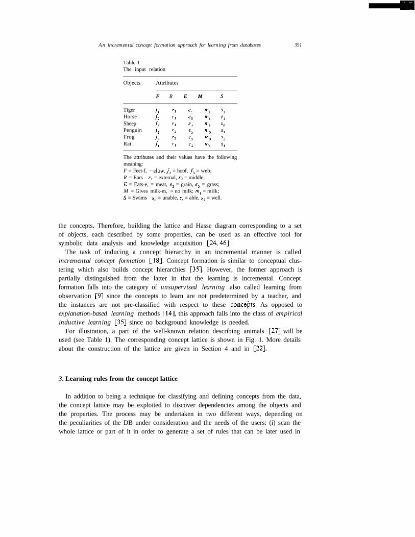
Table 1The input relation
Objects Attributes
F R E M S
TigerHorseSheepPenguinFrogRat
The attributes and their values have the followingmeaning:F = Feet-f, =claw, f, = hoof, f, = web;R = Ears ~ rl = external, rz = middle;E = Eats-e, = meat, e, = grain, e3 = grass;M = Gives milk-m, = no milk; m, = milk;S = Swims -s,, = unable, s1 = able, s2 = well.
the concepts. Therefore, building the lattice and Hasse diagram corresponding to a setof objects, each described by some properties, can be used as an effective tool forsymbolic data analysis and knowledge acquisition [24,46].
The task of inducing a concept hierarchy in an incremental manner is calledincremental concept formation [ 181. Concept formation is similar to conceptual clus-tering which also builds concept hierarchies [35]. However, the former approach ispartially distinguished from the latter in that the learning is incremental. Conceptformation falls into the category of unsupervised learning also called learning fromobservation [9] since the concepts to learn are not predetermined by a teacher, andthe instances are not pre-classified with respect to these concehts. As opposed toexplanation-based learning methods [14], this approach falls into the class of empiricalinductive learning [35] since no background knowledge is needed.
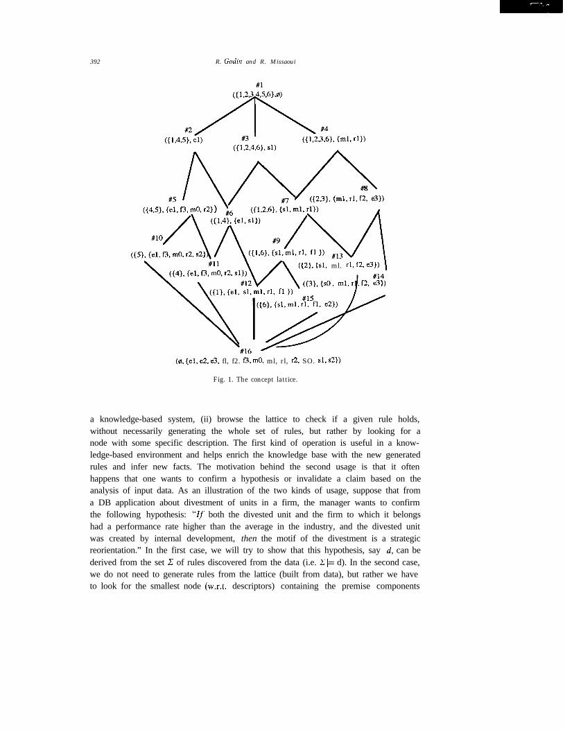
For illustration, a part of the well-known relation describing animals [27] will beused (see Table 1). The corresponding concept lattice is shown in Fig. 1. More detailsabout the construction of the lattice are given in Section 4 and in [22].
3. Learning rules from the concept lattice
In addition to being a technique for classifying and defining concepts from the data,the concept lattice may be exploited to discover dependencies among the objects andthe properties. The process may be undertaken in two different ways, depending onthe peculiarities of the DB under consideration and the needs of the users: (i) scan thewhole lattice or part of it in order to generate a set of rules that can be later used in
392 R. Godin and R. Missaoui
({2). {sl. ml. rl. f2, e3))
(0. {el.e2. e3. fl, f2. f3, m0. ml, rl, R. SO. sl. S21)
Fig. 1. The concept lattice.
a knowledge-based system, (ii) browse the lattice to check if a given rule holds,without necessarily generating the whole set of rules, but rather by looking for anode with some specific description. The first kind of operation is useful in a know-ledge-based environment and helps enrich the knowledge base with the new generatedrules and infer new facts. The motivation behind the second usage is that it oftenhappens that one wants to confirm a hypothesis or invalidate a claim based on theanalysis of input data. As an illustration of the two kinds of usage, suppose that froma DB application about divestment of units in a firm, the manager wants to confirmthe following hypothesis: “Zf both the divested unit and the firm to which it belongshad a performance rate higher than the average in the industry, and the divested unitwas created by internal development, then the motif of the divestment is a strategicreorientation.” In the first case, we will try to show that this hypothesis, say d, can bederived from the set C of rules discovered from the data (i.e. C I= d). In the second case,we do not need to generate rules from the lattice (built from data), but rather we haveto look for the smallest node (w.r.t. descriptors) containing the premise components
An incremental concept Ji,rmation approach ,for learning from databases 393
of that hypothesis, and check if the conclusion components also occur in the intent ofthat node.
In the first case, the learning process is as follows.
Input. A relation or a view of the database.Output. (i) The corresponding concept lattice.
(ii) A set of conjunctive implication rules.Method
Step 1. Construct the concept lattice of the binary relation.Step 2. Generate a set of conjunctive rules from the lattice.Step 3. Remove redundant rules.
Step 2 of the learning process can eiher be handled independently from (but asa sequel to) Step 1 as in Algorithms 4.1 and 4.2 or be integrated with Step 1 as inAlgorithm 4.3.
In the following we use P, Q, R, . , Z to denote sets of properties, while we uselower-case letters p, q, Y, to name atomic properties (descriptors). The notation p qis a simplification of the notation Vx p(x) A q(x) meaning that each object has proper-ties p and q. In the sequel, we shall take the freedom of using either the logical notationor the set-oriented notation, depending on the context under consideration.
The general format of a rule is P*Q, where P and Q represent either a set of objectsor a set of properties. Four cases can be considered:
(i) implication rules for descriptors (IRDS) in which both P and Q belong to Y(9);(ii) implication rules for objects (1~0s) in which both P and Q belong to Y(O);
(iii) discriminant rules for objects (DROS) where PEY(~) and QEY(O);(iv) discriminant rules for descriptors (DRDS) where PEY(O) and Q~g(9).
In the following, we give definitions for implication rules only. Then, we show thatthe rule generation problem is NP-hard. However, under a reasonable assumption,the problem becomes tractable. In Section 4 we propose a set of efficient algorithmsfor implication rule generation.
3.1. Implication rules
We define implication rules (IR) as ones such that P and Q are both subsets of either0 or 9. Due to the nature of IRS, the inference system for functional dependenciesholds also for IRS. The following definitions are borrowed from the implication theoryon functional dependencies [31] and apply to implication rules as well.
Given a set C of IR, the closure C+ is the set of rules implied by C by application ofthe inference axioms. Two sets C and C’ are equivalent if they have the same closure.l P*Q is redundant in the set C of IRS if C- { P=z=Q} I= P*Q.l P*Q is full (or left-reduced) if $ P’cP such that (C- {P=sQ})u{P’+Q} EC.l P*Q is right-reduced if $Q’cQ such that (Z-{P+Q})u{P=Q’j-C.l P*Q is reduced if it is left-reduced and right-reduced, and Q #@.

394 R. Godin and R. Missaoui
l P*Q is trivial if Q G P.l P-Q is elementary if it is full and Ij Q // = 1 and Q Q P.The closure P+ of a set P according to C is defined by: Pi = Pu{ Q IZ G P’ andZ~QEC}.
3.1.1. Conjunctive implication rulesThe problem of generating conjunctive rules can be stated as starting from a finite
model where each atom in the model is denoted by p(a), and finding Horn clauses ofthe form:
VXPl(X)AP,(X)A...AP*(X) =- q(x).
Each pi(X) is a property (descriptor) predicate indicating that x may or may not haveproperty pi. A more accurate notation for pi would be ai( v, where ai is anattribute predicate, and v is a value from the domain of the attribute ai. For example(see Table l), Feet(x)=“f,” is a predicate about webbed animals that we shall writesimply asf3(x) or asf3.
Two alternative notations can be used to express conjunctive implication rules: thecompact form and the Horn clause form. Each (compact) rule P*Q may havea conjunction of properties in the conclusion part, and can equivalently be expressedas II Q II separate Horn clauses P*qi. The compact notation is commonly used in theliterature about machine learning and knowledge discovery [35,43], while the Hornclause notation is frequently adopted in deductive databases and logic programmingstudies [37,41].
Definition 1. A conjunctive implication rule for descriptors (IRD) is an IR of the formD-D’ where D and D’ are subsets of 9. A context (C),9, W) satisfies the IRD D=+-D’ iffor every object x in 0, whenever x is characterized by all the properties found in D ithas necessarily the whole set D’ of properties, i.e.,
f(x) 2 D =+ f(x) 2 D’.
Proposition 1. D=+-D’ is a conjunctive IRD o [[(O”, D”) = inf {(X, X’)E_Y? D c X’ andX#@}]=D’cD”].
In other words, the rule D=z-D’ holds if and only if the smallest concept (w.r.t.properties) containing D as a part of its intent is also described by D’.
Proof. (a) If D=sD’ is computed based on the node described by some couple(O”, D”), it means that the objects in 0” have the properties found in D and D’, andtherefore DUD’ c D”. In particular, D’ c D”. To ensure that every x~c0 that has theproperties in D is also characterized by D’, the couple (O”, D”) must be the smallestconcept containing D.
An incremental concept formation approach ,for learning from databases 395
(c=) Whenever the couple (0”, D”) is the smallest concept containing D, it alsocontains D'. This corresponds exactly to the definition of the IRD: D*D'. 0
Example 1. From the lattice shown in Fig. 1, one can generate the IRDfi*ml y1 s1meaning that if an animal has claws, then it gives milk, has external ears, and is able toswim. This rule is valid since, when starting from the node at the top (i.e. inf(Y)) of thelattice, the first encountered node containing the property fi, which is node #9,contains also the properties m 1, r1 and sl. However, the IRD slam1 does not holdsince node #3 is described by the property s1 alone.
Definition 2. A conjunctive implication rule for objects (IRO) is an IR of the form0-O’ where 0 and 0’ are subsets of 0. A context (0, g,S?) satisfies the IRO 030’ iffor every descriptor x’ in 3, whenever x’ is associated with the objects in 0 it is alsoassociated with the objects in O’, i.e.,
f’(X’)ZO *f’(x’)30’.
For example, the rule dog*(bulldog, poodle} means that bulldogs and poodles have atleast the properties attached to dogs, i.e. they are dogs with possibly additionalcharacterizations. The following proposition is the dual of Proposition 1.
Proposition 2. O*O’ is a conjunctive IRO o [[(0”, D”)=sup{(X, X’)~SplOcx andX’#~}]~O’co”].
In other words, O*O’ if and only if the biggest node (with respect to descriptors)containing 0 as a part of its extent is also described by 0’.
Proof. A reasoning similar to the proof of Proposition 1 can be done to demonstratethe correctness of Proposition 2. 0
Proposition 3. D*D + is a full (or left-reduced) conjunctive IRD if and only ifVQE~QQD*Q+~D+.
Proof. (a) If D-D+ is a full rule, it means that ,JQ CD such that Q=D+. Since theclosure of Q is by definition the set of properties that are implied by Q, then Q*Q’and therefore Q’ CD+.
(-z) Suppose that VQcg [QcD=Q'CD+] holds. As a consequence, Q*D'does not hold, and therefore D-D+ is a full rule. 0
Definition 3. P*Q is an existence implication rule if
$ZcP such that Z+cP+.
A composite rule is one for which the precedent condition does not hold.
396 R. Godin and R. Missaoui
For example, m, =>rl is an existence rule (see the lattice in Fig. 1) while e, ml =wl slfiis a full composite rule since there exists Z= {ml} in the premise P= {e, m,} of thesecond rule such that Z+ c P+, i.e., {m, rl} c e, m, r1 slfi}. Intuitively, an algorithm(that computes existence rules associated with a node H ignores any rule P*Qwhenever there exists at least a subset Z of P such that Z’ is the intent of an ancestornode of H.
NP-hardness of the rule generation problemIt is known that the set-covering problem is an optimization problem that general-
izes and models many NP-complete problems [ 121.An instance (Y, 9) of the set-covering problem contains a finite set Y and a collec-
tion F of subsets Si, . . . , S, of Y, such that every element of Y exists in at least onesubset in 9:
YE u Sisis.9
The problem is to find a minimum-size subset Zg9 such that its members coverthe set Y:
This well-known problem can be useful for proving NP-completeness (and hard-ness) of the rule generation problem which can be stated as starting from a finitemodel where each atom in the model is denoted by p(a), and finding Horn clauses ofthe form:
v’x Pi(X) A Pz(x) A ... A Pm(x)*q(x).
The set Y to be covered corresponds to objects for which property q is false. A setSi in g represents objects for which property pi is false.
Y=O-f’(q)={x~O/q(x)=False}.
Si=jX~YIpi(X)=Fa2Se), 1 didm.
The minimum size cover Z corresponds to the smallest-size union of Si that coversY. In other words,
Z={xEYlpl(x)=False v ... v pm(x)=False}, o r
z=(xEYllpi(x) v ‘.’ VlP,(X)}.
Therefore, we get the following implication:
vxlq(x)~1p,(x)v ... VlP,(X).
The contraposition of the above logical expression leads to the following Horn clause:
v’x Pi(X) A pz(x) A “. A Pm(x)*q(x).
An incremental concrpt formation upprouch .fiw learning jwn databases 391
Since we have shown that the rule generation problem can be reduced to theset-covering problem (which is NP-complete), the rule generation problem is thereforeas hard as finding the minimum-size cover, and hence is an NP-hard problem.
Example: Let us check if e,(x)&m,(x)+f,(x) holds for each object x in Table 1.
Y={x~O~f1(x)=False}=(2,3,4,5}.
The minimum size cover for Y is Z= S,uS,, where:
S,={x~Y~e,(x)=False}={2,3}, and Sz={x~Y~m,(x)=False)={4, 5).
Therefore,
If we assume there exists an upper bound K on the number of descriptors per object,
i.e. IlfC{x>)l/ 6K we limit the size of any rule to contain at most K atoms, andtherefore the problem of rule generation becomes tractable. This assumption is true inthe context of databases since the number of pairs (attribute, value) per row (object) isbounded. Without this restriction, the general problem of rule generation is NP-hardas demonstrated before.
3.1.2. Disjunctive implication rulesDisjunctive implication rules are rules such that either their left-hand side (LHS) or
their right-hand side (RHS) contains a disjunctive expression Qi v ... v Qi vv Qm, where Qi is possibly a conjunction of atomic properties. There is a mapping
between conjunctive and disjunctive rules. The conjunctive IRD d,=aQ can be com-puted from the right-hand disjunctive IRD djaQ1 v ... v Qm by setting Q to theproperties common to Q1 , . . , Qm. The left-hand disjunctive IRD Qi v ... v Q,jdimeans that Qi, . , Qm are the alternative (sets of) properties which subsume di, andcan be computed from the set of conjunctive IRDs (see Algorithm 4.5).
3.2. Characteristic and clussiJicution rules
As mentioned earlier, classification rules discriminate the concepts of one class (e.g.a carnivore) from that of the others, while characteristic rules characterize a classindependently from the other classes. The first kind is a suficient condition of the classunder consideration while the second type is a necessary condition of the class (see [S]for more details).
Implication rules in either conjunctive or disjunctive form can express these two kindsof rules. The RHS disjunctive IRD djaQ1 v ... v Qm may be useful for defining thecharacteristic rule for objects having the property dj, when there is no conjunctive IRDwith dj as a premise. The LHS disjunctive IRD Q1 v ... v Q,adi can be used to definethe cluss$cution rule for objects with the property di. E.g., the classification rule foranimals having claws (propertyf, ) is ez?fl while the characteristic rule for carnivora(property ei) can be expressed by the RHS disjunctive IRD el*fjsl v f3s2 v fi.
398 R. Godin and R. Missaoui
4. Implication rule determination
In [26,46], the authors deal with the problem of extracting rules from the con-cept lattice structure. However, they do not propose any algorithm to determinethose rules. In this section we propose a set of algorithms for rule generation.For ease of exposition, we limit ourselves to IRDs. However, owing to thesymmetry of the lattice structure, the definitions and algorithms can be adaptedwithout difficulty to IROs.
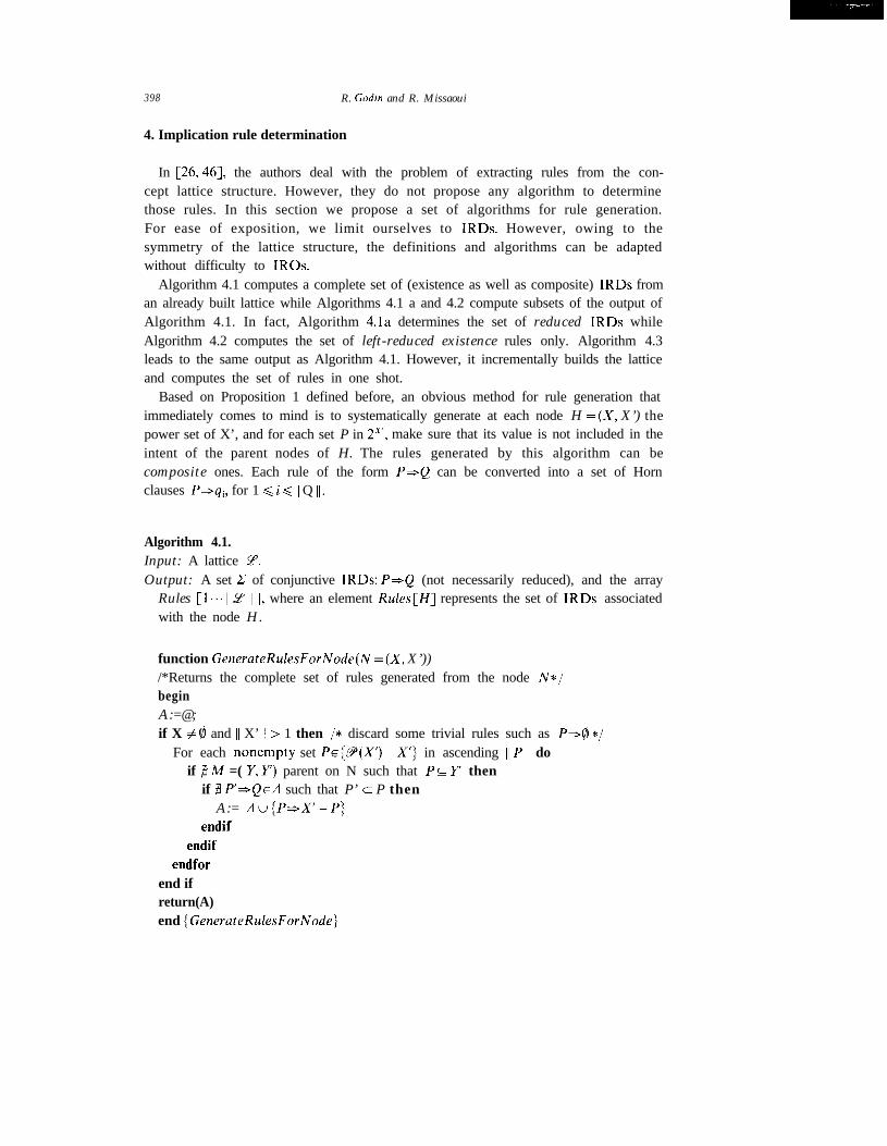
Algorithm 4.1 computes a complete set of (existence as well as composite) IRDs froman already built lattice while Algorithms 4.1 a and 4.2 compute subsets of the output ofAlgorithm 4.1. In fact, Algorithm 4.la determines the set of reduced IRDs whileAlgorithm 4.2 computes the set of left-reduced existence rules only. Algorithm 4.3leads to the same output as Algorithm 4.1. However, it incrementally builds the latticeand computes the set of rules in one shot.
Based on Proposition 1 defined before, an obvious method for rule generation thatimmediately comes to mind is to systematically generate at each node H =(X, X’) thepower set of X’, and for each set P in 2”, make sure that its value is not included in theintent of the parent nodes of H. The rules generated by this algorithm can becomposite ones. Each rule of the form P*Q can be converted into a set of Hornclauses P*qi, for 1 < i < 11 Q /I.
Algorithm 4.1.Input: A lattice _Y.Output: A set C of conjunctive IRDs: P-Q (not necessarily reduced), and the array
Rules [l...li _!Z 111, where an element Ru/es[H] represents the set of IRDs associatedwith the node H.
function GenerateRulesForNode(N =(X, X’))/*Returns the complete set of rules generated from the node N*/beginA:=@;if X #8 and II X’ /I > 1 then /* discard some trivial rules such as P& */
For each nonempty set Pc{Y(X’)-X’} in ascending I/P I/ doif ,3 M =( Y, Y’) parent on N such that PC Y’ then
if $ P’=sQEA such that P’ c P thenA:= Au{P+X’-P}
endifendif
endforend ifreturn(A)end (GenerateRulesForNode}
An incremental concept jiwmution approach fi)r learning ji.om databases 399
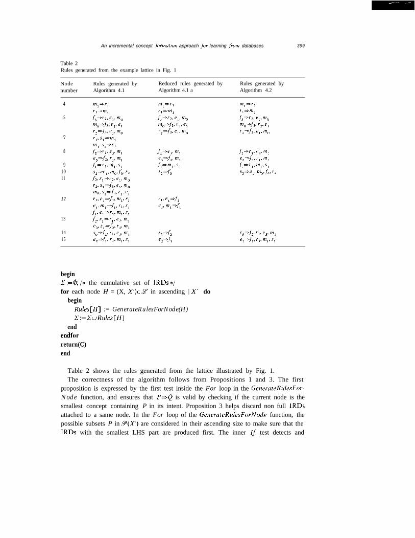
Table 2Rules generated from the example lattice in Fig. 1
Node Rules generated by Reduced rules generated by Rules generated bynumber Algorithm 4.1 Algorithm 4.1 a Algorithm 4.2
4
5
8
91011
12
13
1415
ml*rl
f-,-m,.f,-r2, e,, m,mO=f3, rz, e,rzqf3, e,, m,
m,=rlrl*mlf3-rz, e,. m,m,*f3, rz3 e,r,*fi e,, m,
sOsf2,rl, e3, m,e,+f;, rl, m,, s,
beginC :=& /* the cumulative set of IRDs */for each node H = (X, X’)E_Y in ascending I/X’ 11 do
beginRules[H] := GenerateRulesForNode(H)C:=CuRules[H]
endendforreturn(C)end
Table 2 shows the rules generated from the lattice illustrated by Fig. 1.The correctness of the algorithm follows from Propositions 1 and 3. The first
proposition is expressed by the first test inside the For loop in the GenerateRulesFor-Node function, and ensures that P*Q is valid by checking if the current node is thesmallest concept containing P in its intent. Proposition 3 helps discard non full IRDsattached to a same node. In the For loop of the GenerateRulesForNode function, thepossible subsets P in 9(X’) are considered in their ascending size to make sure that theIRDs with the smallest LHS part are produced first. The inner Zf test detects and
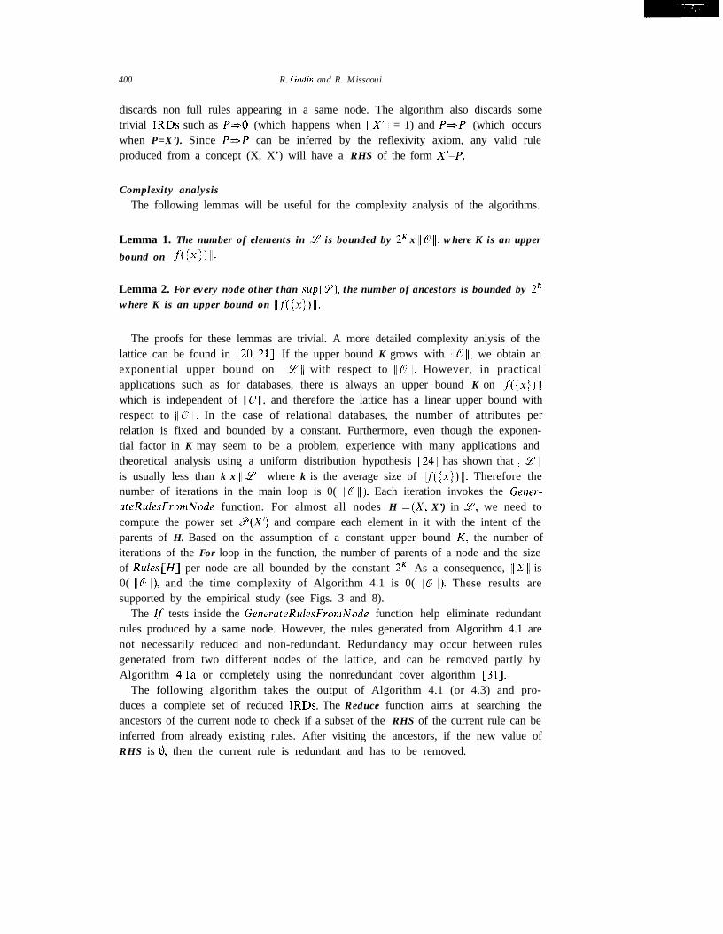
400 R. Godin and R. Missaoui
discards non full rules appearing in a same node. The algorithm also discards sometrivial IRDs such as P*@ (which happens when /IX’ I/ = 1) and P*P (which occurswhen P=X’). Since P*P can be inferred by the reflexivity axiom, any valid ruleproduced from a concept (X, X’) will have a RHS of the form X’-P.
Complexity analysisThe following lemmas will be useful for the complexity analysis of the algorithms.
Lemma 1. The number of elements in 9 is bounded by 2K x 116 11, where K is an upper
bound on Ilf({~>,ll.
Lemma 2. For every node other than sup(T), the number of ancestors is bounded by 2Kwhere K is an upper bound on Ilf({x})ll.
The proofs for these lemmas are trivial. A more detailed complexity anlysis of thelattice can be found in [20,21]. If the upper bound K grows with 110 11, we obtain anexponential upper bound on 11 Yl/( with respect to IlO 11. However, in practicalapplications such as for databases, there is always an upper bound K on lif({x})llwhich is independent of 11~5 11, and therefore the lattice has a linear upper bound withrespect to /I 0 11. In the case of relational databases, the number of attributes perrelation is fixed and bounded by a constant. Furthermore, even though the exponen-tial factor in K may seem to be a problem, experience with many applications andtheoretical analysis using a uniform distribution hypothesis [24] has shown that 119 11is usually less than k x II_YIl where k is the average size of Ilf({x})ll. Therefore thenumber of iterations in the main loop is 0( 11 G 11). Each iteration invokes the Gener-ateRulesFromNode function. For almost all nodes H =(X, X’) in 9, we need tocompute the power set 9(X’) and compare each element in it with the intent of theparents of H. Based on the assumption of a constant upper bound K, the number ofiterations of the For loop in the function, the number of parents of a node and the sizeof Rules[H] per node are all bounded by the constant 2K. As a consequence, I( C I/ is0( IlGlI), and the time complexity of Algorithm 4.1 is 0( IIC 11). These results aresupported by the empirical study (see Figs. 3 and 8).
The Zf tests inside the GenerateRulesFromNode function help eliminate redundantrules produced by a same node. However, the rules generated from Algorithm 4.1 arenot necessarily reduced and non-redundant. Redundancy may occur between rulesgenerated from two different nodes of the lattice, and can be removed partly byAlgorithm 4.la or completely using the nonredundant cover algorithm [31].
The following algorithm takes the output of Algorithm 4.1 (or 4.3) and pro-duces a complete set of reduced IRDs. The Reduce function aims at searching theancestors of the current node to check if a subset of the RHS of the current rule can beinferred from already existing rules. After visiting the ancestors, if the new value ofRHS is 8, then the current rule is redundant and has to be removed.

An incremental concept formation approach for learning from databases 401
Algorithm 4.laInput: A lattice 9, and the array Rules [ 1 . . . I/ 2 I/ ] generated by Algorithm 4.1 (or 4.3)
where an element Rules[H] represents the set of rules associated with the node Hin 9.
Output: A complete set C of conjunctive and reduced IRDs: P=Q
function Reduce(H) /* Returns a set of reduced rules corresponding to node H*/function CheckParents(N, LHS, RHS)begin
for each parent M = (Y, Y’) of N such that LHSn I” # 8 dofor each rule P*Q in Rules[M] do
if P C {LHSURHS} thenRHS:= RHS-Q /* the common part to RHS and Q is redundant */
endifendforCheckParents(M, LHS, RHS)
endforend (CheckParents}
begin {Reduce}A := 0; /* The set of IRDs for the current node */for each rule P=>QERules[H] do
CheckParents(H, P, Q);If Q # 0 then /* Q = 0 means that the initial rule is redundant */
d := du{P*Q}endif
endforreturn(d)
end {Reduce}begin
C := 0; /* the cumulative set of IRDs */for each node H = (X, X’)E~ do
C:= CuReduceendforreturn(C)
end
Complexity analysisBased on Lemmas 1 and 2, the number of iterations in the main procedure is linear
with respect to the size of 0, and each call of the function Reduce is done in a constanttime since the number of ancestors of a node is bounded by 2K. Therefore, the timecomplexity of Algorithm 4.1 a is 0 ( II0 /I ), which is supported by the empirical analysispresented in Section 5.
402 R. Godin and R. Missaoui
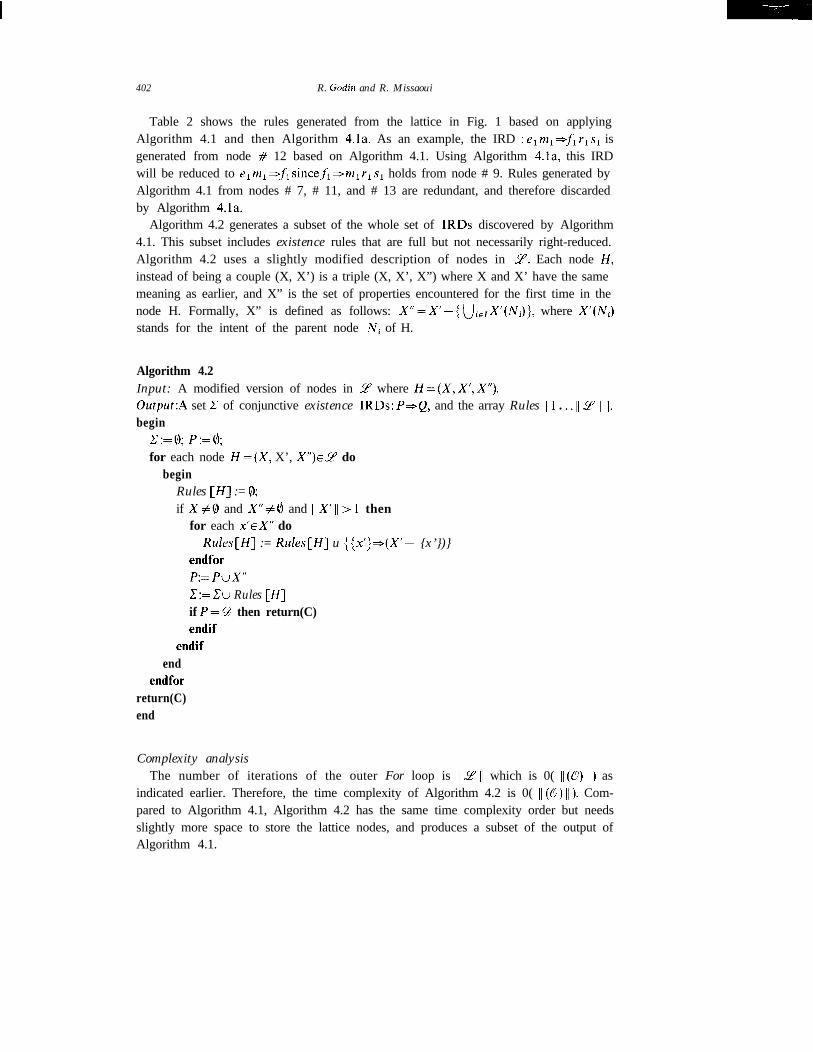
Table 2 shows the rules generated from the lattice in Fig. 1 based on applyingAlgorithm 4.1 and then Algorithm 4.la. As an example, the IRD : elm,=-fIrIs, isgenerated from node # 12 based on Algorithm 4.1. Using Algorithm 4.la, this IRDwill be reduced to e, m, *fi sincef, *m, rl s1 holds from node # 9. Rules generated byAlgorithm 4.1 from nodes # 7, # 11, and # 13 are redundant, and therefore discardedby Algorithm 4.la.
Algorithm 4.2 generates a subset of the whole set of IRDs discovered by Algorithm4.1. This subset includes existence rules that are full but not necessarily right-reduced.Algorithm 4.2 uses a slightly modified description of nodes in L??. Each node H,instead of being a couple (X, X’) is a triple (X, X’, X”) where X and X’ have the samemeaning as earlier, and X” is the set of properties encountered for the first time in thenode H. Formally, X” is defined as follows: X”=X’-{ UislX’(Ni)}, where X’(Ni)stands for the intent of the parent node Ni of H.
Algorithm 4.2Input: A modified version of nodes in _Y where H=(X, X’,X”).0utput:A set C of conjunctive existence IRDs: PaQ, and the array Rules [l . . .I1 2 111.begin
C:=@; P:=@;for each node H =(X, X’, X”)E_Y do
beginRules [If] := 0;if X#8 and X”#@ and IIX’ll>l then
for each x’EX” doRules[H] := Rules[H] u { {x’}*(X’- {x’})}
endforP:= PUX”C:= Cu Rules [If]if P=9 then return(C)endif
endifend
endforreturn(C)end
Complexity analysisThe number of iterations of the outer For loop is lIL.2’ I/ which is 0( II(O) 11) as
indicated earlier. Therefore, the time complexity of Algorithm 4.2 is 0( II (Co) I/ ). Com-pared to Algorithm 4.1, Algorithm 4.2 has the same time complexity order but needsslightly more space to store the lattice nodes, and produces a subset of the output ofAlgorithm 4.1.
An incremental concept jbrmation approach for learning from databases
(0. {el. e2. e3. fl, f2, f3. m0. ml. rl. r2. SO. sl. ~2))
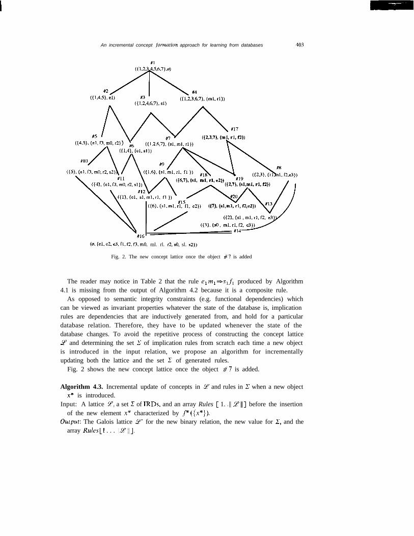
Fig. 2. The new concept lattice once the object #7 is added
The reader may notice in Table 2 that the rule e, m, =-slfi produced by Algorithm4.1 is missing from the output of Algorithm 4.2 because it is a composite rule.
As opposed to semantic integrity constraints (e.g. functional dependencies) whichcan be viewed as invariant properties whatever the state of the database is, implicationrules are dependencies that are inductively generated from, and hold for a particulardatabase relation. Therefore, they have to be updated whenever the state of thedatabase changes. To avoid the repetitive process of constructing the concept lattice9 and determining the set C of implication rules from scratch each time a new objectis introduced in the input relation, we propose an algorithm for incrementallyupdating both the lattice and the set C of generated rules.
Fig. 2 shows the new concept lattice once the object #7 is added.
Algorithm 4.3. Incremental update of concepts in 3 and rules in C when a new objectx* is introduced.
Input: A lattice 9, a set C of IRDs, and an array Rules [ 1. .I1 $P I/ ] before the insertionof the new element x* characterized by f* ({x*}).
Output: The Galois lattice 9” for the new binary relation, the new value for C, and thearray Rules[l . . . /l_%/l].

404 R. Godin and R. Missaoui
Procedure SelectAndClassifyNodesProcedure Search(H = X, X’))begin
Mark H as visited and add H to C[ 11X’(H) ii];for each Hd child of H
if Hd is not marked as visitedSearch(H,)
endifendfor
end {Search}function GenerateRulesForNode (N=(X, X’)) /* See Algorithm 4.1 */
end {GenerateRulesForNode}begin
Mark inf(_F) as visited and add inf(9) to C[ IlX’(inf(.T))il]for each x’E~* ({x*})
Search (Px.)endfor
end {SelectAndClassifyNodes}
begin1. Adjust sup(L?) for new elements in 9’2. if sup(_Y)=(@, 0) then3. Replace SUP(~) by: H=(x*,f* ({x*}));4. for each x’~f* ({x*}) do
Make P,, point to Hendfor
5. Rules[H] := GenerateRulesForNode[H]6. C := Cu Rules [H]7. else8. iff*({x*})q X’(sup(9)) then9. if X(sup(Y))=@ then
10. for each x’~f+ ({x*}) such that x’$(sup(Z)) doMake P,, point to sup(9’)endfor
11. X’(suP(=W):=X’(suP(~))u,f+({x*))12. else13. Add a new node H =(8, X’(sup(LZ?))uf* (ix*})) /* H becomes sup(Z) */14. Add a new edge (sup(Y),H)15. endif16. endif17. SelectAndClassifyNodes;
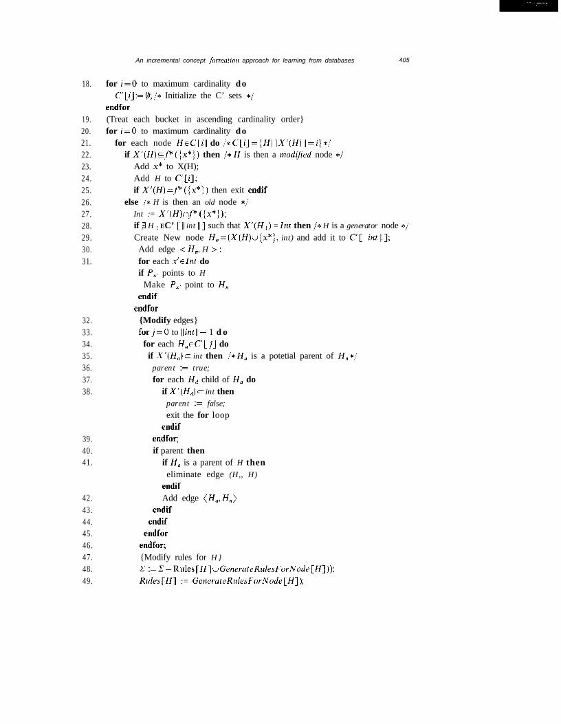
An incremental concept fbrmation approach for learning from databases 405
18.
19.20.21.22.23.24.25.26.27.28.29.30.31.
32.33.34.35.36.37.38.
39.40.41.
42.43.44.45.46.47.48.49.
for i=O to maximum cardinality doC’[i]:= 0; /* Initialize the C’ sets */
endfor(Treat each bucket in ascending cardinality order}for i=O to maximum cardinality do
for each node HgC[i] do /* C[i]={Hl IlX’(H)II =i} */if X’(H)cf” (ix*}) then /* H is then a modijed node */
Add x* to X(H);Add H to C’[i];if X’(H)=f* ({x*}) then exit endif
else /* H is then an old node */Int := X’(H)nf* ({x*});if j3 H 1 EC’ [ // int II ] such that X’(H 1) = Znt then /* H is a generator node */Create New node H,=(X(H)u{x*}, int) and add it to C’[ Ilintll];Add edge < H,, H > ;for each x’glnt doif P,, points to H
Make P,, point to H,endif
endfor{Modify edges}forj=O to Ilintl~ - 1 d o
for each H,EC’ [ j] doif X’(H,) c int then /* H, is a potetial parent of H, */
parent := true;for each Hd child of H, do
if X’(H,) c int thenparent := false;exit the for loop
endifendfor;if parent then
if H, is a parent of H theneliminate edge (H,, H)
endifAdd edge (H,, H,)
endifendif
endforendfor;{Modify rules for H}C :=C-Rules[H]uGenerateRulesForNode[H]));Rules[H] := GenerateRulesForNode[H]);
406 R. Godin and R. Missaoui
50. Rules[H,,] := GenerateRulesForNode(H,);51. C := Cu Rules [HJ;52. if int =f* ({x*}) then exit endif53. endif54. endif55. endfor56. endfor57. endifend
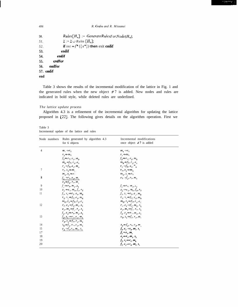
Table 3 shows the results of the incremental modification of the lattice in Fig. 1 andthe generated rules when the new object #7 is added. New nodes and rules areindicated in bold style, while deleted rules are underlined.
The lattice update processAlgorithm 4.3 is a refinement of the incremental algorithm for updating the lattice
proposed in [22]. The following gives details on the algorithm operation. First we
Table 3Incremental update of the lattice and rules
Node numbers Rules generated by algorithm 4.3 Incremental modificationsfor 6 objects once object #7 is added
4
7
8
91011
12
13
141517181920
f,==-,, m,, s1
s2-el, m,,f3, r2f& s1*r2, e,, m,r2, s,-f3, e,, m,mO, sI*f3, r2, e,rl, e,-f,, m,, s,e,, m,*fI, rl, s1f,, e,==-r,, m,, s1e3, s,-fi, rI, m1

An incremental concept formation approach for learning from databases 407
explain how the lattice is incrementally updated, an then we look at the rule updating.The lattice 2’ can be obtained from Y by taking all the nodes in S? and modifying theX part of the nodes for which X’cf * (Ix*}) by adding x*. The nodes that remainunchanged are called old nodes (nodes #2,5,6,&g, 10, 11, 12, 13, 14, 15, and 16 n Fig.2) and the other ones are called modijied nodes in dp’ (nodes # 1, 3, 4, and 7). Inaddition, new nodes are created (nodes # 17, 18, 19,20). These new nodes are alwaysin the form (Yu Ix*}, Y’nf * (ix*}) for some node (Y, Y’) in LZ’. They correspond tonew X’ sets with respect to 2. The related (Y, Y’) node in 2 is called the generator forthis new node. If the generators can be characterized in some manner, the new nodescan be generated from them. Proposition 4 is one possible characterization, and isused implicitly in Algorithm 4.3. This proposition is rather obvious but formal proofsare found in [22].
Proposition 4. If (X, X’)=inf {(Y, Y’)ELZ~X’= Y’nf*({x*})} for some set X’ andthere is no node of the form (Z, X’) in _%’ then (Y, Y’) is the generator of a new node(X= Yu{x*}, X’= Y’nf*({X*}))Es?.
Any new X’ set in _C?” will have to be the result of intersecting f * ({x*}) with someY’ set already present in the lattice 2. There may be many nodes in S? that givea particular new intersection in this manner. For example, in Fig. 2, the new X’ set,{m,, rl, f2} corresponding to the new node # 17 can be formed by intersectingf*({x*})={sl, m,, rl,fz, e2} with the Y’ set of node #8 which is {rI, m,,f& e3}, orthe Y’ set of node # 14 which is {so, ml, rl, fi, e3}. However, there is only one ofthese nodes that is the generator of the new node. It corresponds to the smallestold node that produces the intersection. Unicity of the greatest lower bound isguaranteed by the fondamental theorem (see Section 2). In Fig. 2, the generatornodes for the new nodes # 17, # 18,# 19, and #20 are #8,# 15, # 13, and # 16respectively.
One minor problem is for the case of the generator being sup(6p) =(@, 9). If the newinstance x* contains new features not contained in 9, there will be no generators forthe node ({x*}, f * ({x*}). In practical applications, we may want CS to grow as newfeatures are encountered. This is easily taken into account by simply adding the newfeatures to 9 as a first step in the algorithm, and therefore the characterizationremains valid.
Besides updating the nodes, the edges of the Hasse diagram also have to be takencare of. First, the generator of a new node will always be a child to the new node in theHasse diagram. The children of old nodes do not change. The parents of generatornodes, however, have to be changed. The generator is the only old node that becomesa child of a new node. There may be another child but it will be a new node. Forexample in Fig. 2, there is an edge from the new node # 17 to its generator # 8 andthere is another child # 19 which is a new node. The parents of old nodes that are notgenerators remain unchanged.
408 R. Godin and R. Missaoui
Moreover, the parents of modified nodes never change. However, the children ofsome modified nodes may change. There may be new children that are new nodes.This implies that some old children have to be removed if the new children fall inbetween the old child and the modified node. This is the case when the new node fallsbetween a generator and one of its parents. The result is that the edge from that parentto the generator (e.g., edge (# 7, # 13) in Fig. 2) is replaced by two edges, one from theparent to the new node (i.e., edge (#7, # 19)) and one from the new node to thegenerator (i.e., edge (# 19, # 13)).
Table 4 is a summary of the modifications resulting from the update process withrespect to our categorization of nodes. The impact of the update on the X set, the X’set, the parents and children are shown in the four columns of the table. The first threecategories (rows) represent the nodes that are in _P and remain in dp’ with possiblysome modifications. Cases 1 and 2 need the update of nodes or edges. The fourth caseconcerns new nodes.
The lattice is initialized with one element: (0, 8). This means that 0 =S+ =0. Thealgorithm updates 0 and 3 as new elements are added. If we assume that 0 and9 contain in advance every element with an empty 9, the lattice would be initial-ized with the two elements: (6, 0) and (0, 9). This would slightly simplify the algo-rithm because adjusting 9 by adding new elements from f* (ix*}) would not benecessary.
Lines 1-16 of the main procedure essentially take into account the case when newproperties appear by adjusting 9 in sup(T). Line 17 calls the SelectAndClassifyNodesprocedure. This procedure does the following tasks:
(1) First, it selects a subset of nodes from the lattice for the updating process, i.e. thenodes which have at least one property in common with the new object because theother nodes have no effect on the update process. The result is a huge saving asopposed to searching the whole lattice. To perform the selection without having toscan the whole lattice, for each x’ in 9 a pointer P,, on the smallest node containing x’is maintained and these pointers are used as entry points for a top-down depth-firstsearch starting with every x’ inf* ({x*}). This guarantees that any node encounteredwill have at least x’ in common withf* (Ix*}). Maintaining these pointers is expressedin lines 4, 10 and 31 of the algorithm.
(2) Second, the nodes are sorted into buckets C[ 11 X’ II] of same cardinality (1 X’ I/because the following part of the algorithm needs to work level by level based on
IIX’II.The main loop (lines 20-56) iterates on the nodes selected in SelectAndClas-
sifyNodes by going through the C buckets in ascending /I X’ 11. Lines 22-25 process themodified nodes. When the condition in line 25 holds, the rest of the treatment isskipped because the nodes under consideration cannot be generators. New nodes areobtained by systematically trying to generate a new intersection from each pair (Y, Y’)already in the lattice by intersecting Y’ with f* (ix*)) (line 27). Verifying that thisintersection is not already present is done by looking at the sets already encountered
An incremental concept formation approach for learning from databases 409
which are subsets off* ({x*}) (line 28). These sets are kept in C’ (line 24, line 29). Thisis valid only because the nodes are treated in ascending /I X’ I/. Furthermore, the firstnode encountered which gives a new intersection is the generator of the new nodebecause it is necessarily the infimum. Thus, we compute the X set of the new node byadding x* to the generator’s X set (line 29). Also, there is automatically an edge fromthe new node to the generator as explained earlier (line 30). When a new node is added,some edges have to be added from modified or other new nodes to the new node. Thecandidates are necessarily in the C’ sets since their X’ set must be a subset off* ({x*}).These parents of the new node are determined by examining the nodes in C’ (lines3246) testing if the X’ sets are subsets of the X’ set of the new node (line 35) andverifying that no child of the potential parent has this property (lines 36-39). It isnecessary to eliminate an edge between the new parent and the generator when thereis such an edge (lines 41 and 42).
The rule update processThe rule updating process is very simple compared to the lattice updating part.
Algorithm 4.3 computes the same set of rules as Algorithm 4.1 and uses the sameprocedure for finding rules of a node, that is GenerateRulesForNode. As in Algorithm4.1, the rules are related to the node which generates them, and represented by anarray Rules[l . . . I/ 9 111. The GenerateRulesForNode procedure, as previously ex-plained, finds the rules by looking at the parents of the current node. So the non newnodes which might have their rule set altered by the update operation are thegenerator nodes since their parents are altered (see Table 4). The rules for generator(old) nodes are treated in lines 47-49 where the old set of rules is replaced by the new
Table 4Summary of the modifications of the update process
Type of node
1. Modified node(Y, Y’)EG
X set
Add x*
X’ set Parents Children
No change No change Add new nodes insome cases. Removea generator whena new node in between
2. Old node generator of N No change No change Add new node N No changeand remove parentwhen N is in betweenthis parent and thegenerator
3. Old node non-generator of N
No change No change No change No change
4. New node havinggenerator (Y, Y’)
Yu{x*} r’nf( ix*}) Old nodes and new Generator andnodes possibly new node
410 R. Godin and R. Missaoui
set computed from the GenerateRulesForNode function. There are also new ruleswhich might be generated from the new nodes. This is done in lines 50 and 51 of thealgorithm using the same GenerateRulesForNode function. Lines 5 and 6 take care ofthe special case for the first object added to the lattice.
Complexity analysisThe time complexity of iterating on the nodes for creating the intersections and
verifying the existence of the intersection in C’ is the major factor in analyzing thecomplexity of the algorithm. Although the linking process is a bit tedious, the numberof nodes affected is bounded by 2K and this part is only done when a generator node isencountered. This is why we give a fairly straight-forward algorithm for this process.The rule generation is done only for generators and new nodes. Given the upperbound K, the number of nodes treated is 0( 110 II), // C’ 11 is bounded by 2K, the numberof generators and new nodes are also bounded by 2K and the rule generation usingGenerateRulesForNode is also bounded by a constant as explained earlier. Thereforethe total process is 0( I/O II).
We have proposed so far algorithms for generating rules in conjunctive forms. Inthe following we present procedures aimed at detecting rules in (exclusive) disjunctiveforms as well.
Algorithm 4.4.Input: A descriptor dj in 9, and a lattice 9.Output: A disjunctive RHS rule of the form dj+Q1 v ... v Q,,,.beginRHS := True;
for each parent node Ni of sup(Y) such that X(sup(Z))=0 doif djsX’(Ni) then /* X’(Ni) stands for the intent of Ni */
RHS:= RHS V (X’(Ni)-{dj})endif
endforreturn(dj*RHS)end
To collect the disjunction of the different conjunctions of descriptors that dj implies,Algorithm 4.4 selects all the parent nodes Ni of sup(Y) such that these nodes includedj in their intent, and then takes the descriptors other than dj. This algorithm is 0 110 /Iand is particularly useful when there is no (nontrivial) conjunctive IRD with dj asa premise. E.g., the characterist ic rule for carnivora is e,+f3m0r,sl v
bbr2s2 vfislmlrl which can be simplified (using existing IRDs) intoel+f3s1 vf3s2 vfi, meaning that carnivora are either webbed animals able to swim,or animals with claws.
An incremental concept .formation approach ,fiw learning ,fk)m databases 41 I
Algorithm 4.5Input: A descriptor di in 9, and a set C of conjunctive IRDs.Output: The disjunctive LHS rule Q1 v ... v Q,=di.beginOld := 0; New I= di; LHS:= True;
while Old # New or C # $!I dobeginOld:= New
for each {P~Q}EC doif 3SE New such that Q c S thenbegin
C:= Z- {P+Q}New := N e w u { P u ( S - Q ) }L H S : = L H S v {Pu(S-Q)}
endendif
endforend
endwhilereturn (LHS~di)end
This algorithm implicitly uses the same inference axioms as those related tofunctional dependencies to derive all the alternative Qj that imply a discriptor di. Forexample, if dj=f and C = { a*b; bcdd; kde; d*e; eaf}, then Algorithm 4.5 willproduce e v d v k v bc v ac*$
Complexity analysis
The While needs about 119 // iterations while the For loop is executed 11 C 11 times.Therefore, the overall complexity is 0( 11% /I x I/ Cf 11) which is reduced to 0( l(c 11)if the assumption of a fixed bound K on the number of descriptors per objectis retained.
5. Empirical analysis of the algorithms
The algorithms described in Section 4 have been implemented in Smalltalk withinthe environment of ObjectWorks (release 4.0). The prototype runs both on SUNSPARC work-stations and MacTntosh micro-computers equipped with 16 Mega-bytes RAM. The empirical comparison of the algorithms has been undertaken fora real-life application. The application concerns a data repository for a large databasedescribing more than four thousand of attributes by means of a set of keywords, and
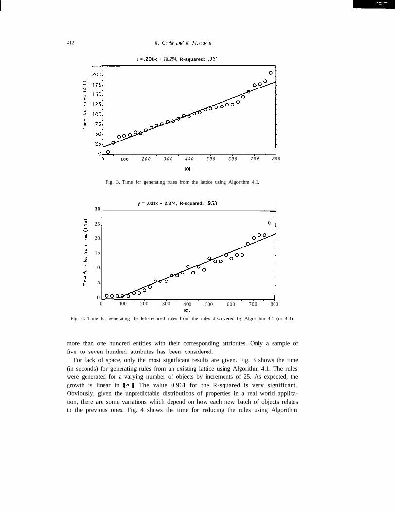
412 R. Godin und R. Missuoui
v = .206x + 18.284, R-squared: .961
00. , . , . , . , . , . , . , ,0 100 2 0 0 3 0 0 4 0 0 5 0 0 6 0 0 7 0 0 8 0 0
11011
Fig. 3. Time for generating rules from the lattice using Algorithm 4.1.
30y = .031x - 2.374, R-squared: .953
? 25 1 0 tz42 20.
E.i? 15.
P2= 10.z
Eiz 5.
0 , 000 100 200 300 400 500 600 700 800
Fig. 4. Time for generating the left-reduced rules from the rules discovered by Algorithm 4.1 (or 4.3).
more than one hundred entities with their corresponding attributes. Only a sample offive to seven hundred attributes has been considered.
For lack of space, only the most significant results are given. Fig. 3 shows the time(in seconds) for generating rules from an existing lattice using Algorithm 4.1. The ruleswere generated for a varying number of objects by increments of 25. As expected, thegrowth is linear in 110 /I. The value 0.961 for the R-squared is very significant.Obviously, given the unpredictable distributions of properties in a real world applica-tion, there are some variations which depend on how each new batch of objects relatesto the previous ones. Fig. 4 shows the time for reducing the rules using Algorithm
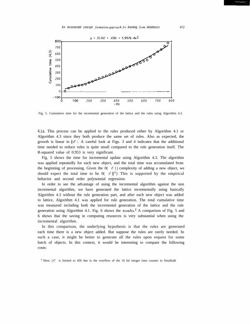
An incremental concept ,fbrmation upproach jbr learning .fiom databases 413
y = 35.542 + .438x + 5.997E-4x28001 ot700.
600.
500.
400.
300.
200.
100.
0. _.o-_______ .ll_l .__...... - 11~ ._._.“.._ _.....
-1004 . , . , . , . , . , . , . , . 40 100 2 0 0 3 0 0 4 0 0 5 0 0 6 0 0 7 0 0 8 0 0
Fig. 5. Cumulative time for the incremental generation of the lattice and the rules using Algorithm 4.3.
4.la. This process can be applied to the rules produced either by Algorithm 4.1 orAlgorithm 4.3 since they both produce the same set of rules. Also as expected, thegrowth is linear in 110 11. A careful look at Figs. 3 and 4 indicates that the additionaltime needed to reduce rules is quite small compared to the rule generation itself. TheR-squared value of 0.953 is very significant.
Fig. 5 shows the time for incremental update using Algorithm 4.3. The algorithmwas applied repeatedly for each new object, and the total time was accumulated fromthe beginning of processing. Given the 0( 116) I/ ) complexity of adding a new object, weshould expect the total time to be 0( 110 l12). This is supported by the empiricalbehavior and second order polynomial regression.
In order to see the advantage of using the incremental algorithm against the nonincremental algorithm, we have generated the lattice incrementally using basicallyAlgorithm 4.3 without the rule generation part, and after each new object was addedto lattice, Algorithm 4.1 was applied for rule generation. The total cumulative timewas measured including both the incremental generation of the lattice and the rulegeneration using Algorithm 4.1. Fig. 6 shows the results.2 A comparison of Fig. 5 and6 shows that the saving in computing resources is very substantial when using theincremental algorithm.
In this comparison, the underlying hypothesis is that the rules are generatedeach time there is a new object added. But suppose the rules are rarely needed. Insuch a case, it might be better to generate all the rules upon request for somebatch of objects. In this context, it would be interesting to compare the followingcosts:
* Here, I/ 6 11 is limited to 450 due to the overflow of the 16 bit integer time counter in Smalltalk
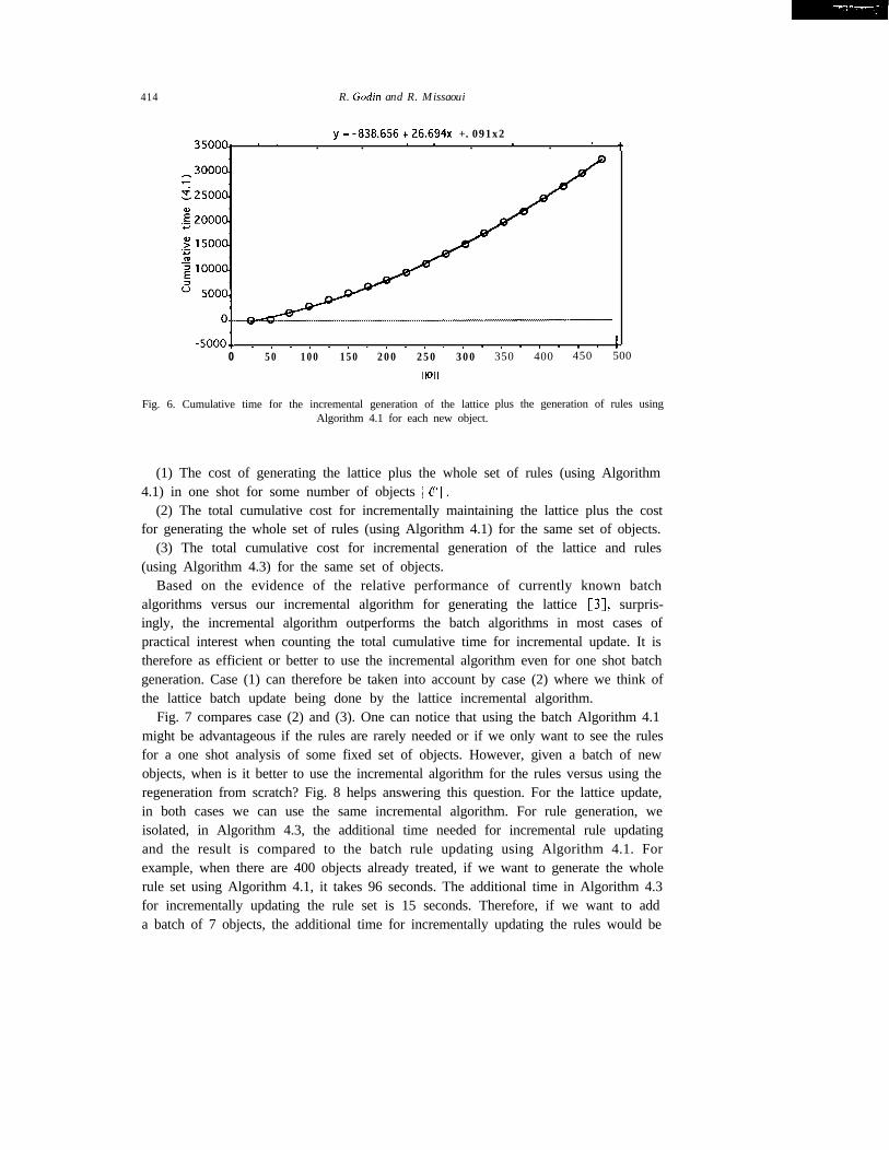
414 R. Godin and R. Missaoui
y=-838.656+26.694x +.091x235ooaf *. . . ' ' . * . ' t
-5oool . , . , . , . , . , . , . , . , . , . 1350 400 450 5000 50 100 150 200 250 300
11011
Fig. 6. Cumulative time for the incremental generation of the latticeAlgorithm 4.1 for each new object.
plus the generation of rules using
(1) The cost of generating the lattice plus the whole set of rules (using Algorithm4.1) in one shot for some number of objects /I CO 11.
(2) The total cumulative cost for incrementally maintaining the lattice plus the costfor generating the whole set of rules (using Algorithm 4.1) for the same set of objects.
(3) The total cumulative cost for incremental generation of the lattice and rules(using Algorithm 4.3) for the same set of objects.
Based on the evidence of the relative performance of currently known batchalgorithms versus our incremental algorithm for generating the lattice [3], surpris-ingly, the incremental algorithm outperforms the batch algorithms in most cases ofpractical interest when counting the total cumulative time for incremental update. It istherefore as efficient or better to use the incremental algorithm even for one shot batchgeneration. Case (1) can therefore be taken into account by case (2) where we think ofthe lattice batch update being done by the lattice incremental algorithm.
Fig. 7 compares case (2) and (3). One can notice that using the batch Algorithm 4.1might be advantageous if the rules are rarely needed or if we only want to see the rulesfor a one shot analysis of some fixed set of objects. However, given a batch of newobjects, when is it better to use the incremental algorithm for the rules versus using theregeneration from scratch? Fig. 8 helps answering this question. For the lattice update,in both cases we can use the same incremental algorithm. For rule generation, weisolated, in Algorithm 4.3, the additional time needed for incremental rule updatingand the result is compared to the batch rule updating using Algorithm 4.1. Forexample, when there are 400 objects already treated, if we want to generate the wholerule set using Algorithm 4.1, it takes 96 seconds. The additional time in Algorithm 4.3for incrementally updating the rule set is 15 seconds. Therefore, if we want to adda batch of 7 objects, the additional time for incrementally updating the rules would be
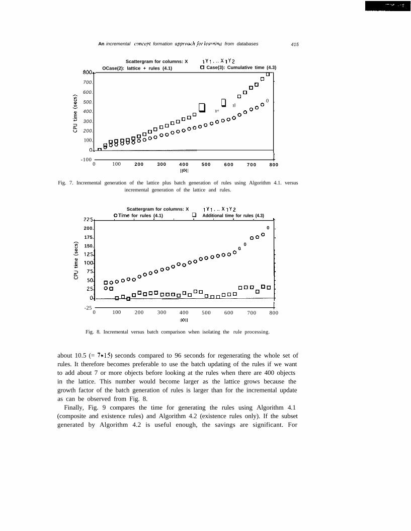
An incremental concept formation approach,for learning from databases 415
800~
700.
600.
500.
400.
300.
200.
100.
0,
Scattergram for columns: X lY1 . ..XlY2
OCase(2): lattice + rules (4.1) 0 Case(3): Cumulative time (4.3)
00 _
on0
0
q n00 .
q n+O0
oo” .
ooo”oo”
-100 t0 100 200 300 400 500 600 700 800
11011
Fig. 7. Incremental generation of the lattice plus batch generation of rules using Algorithm 4.1. versusincremental generation of the lattice and rules.
Scattergram for columns: X lY1 . ..XlY2OTime for rules (4.1) q Additional time for rules (4.3)
225a ’ ’ ’ ’ n ’ ’ - L200. 0 .175. oOO -150. 0
0
-25 t0 100 200 300 400 500 600 700 800
11011
Fig. 8. Incremental versus batch comparison when isolating the rule processing.
about 10.5 (= 7*15) seconds compared to 96 seconds for regenerating the whole set ofrules. It therefore becomes preferable to use the batch updating of the rules if we wantto add about 7 or more objects before looking at the rules when there are 400 objectsin the lattice. This number would become larger as the lattice grows because thegrowth factor of the batch generation of rules is larger than for the incremental updateas can be observed from Fig. 8.
Finally, Fig. 9 compares the time for generating the rules using Algorithm 4.1(composite and existence rules) and Algorithm 4.2 (existence rules only). If the subsetgenerated by Algorithm 4.2 is useful enough, the savings are significant. For

416 R. Godin und R. Missaoui
Scattergram for columns: X lY1 . ..XlY2
225~OTime for rules (4.1) q Time for rules (4.2)
- . - . * . * . * . I.200. 0 .
175. oo” -3 0: 150- 03 125. 0.g 100. oooooO
r2 75. 00
oooOo
w50.
oooO
00 000
25- 0
0_~..8.~.D~.96.e.~~~~~.~~~.~.~~~.n.~.n.~~~~~~.~.
- 2 5 , . , . , . , . , . , . , . , . ,-0 100 200 300 400 500 600 700 800
11011
Fig. 9. Time for generating the rules from the lattice using Algorithm 4.1 versus Algorithm 4.2.
Algorithm 4.2, the time is less than two seconds as opposed to [6 . . .205] range forAlgorithm 4.1.
6. Conclusion
We have proposed an approach based on the concept lattice structure to discoverconcepts and rules related to the objects and their properties. This approach has beentested on many data sets found in the literature and has been proved to be as efficientand effective as some works related to knowledge mining [S, 431. For example, allrules that can be generated by algorithms in [S, 271 are also produced by ouralgorithms. The algorithms presented in this paper have also been tested on real-lifeapplications [25].
Our approach to rule generation can be very useful in database applications fordiscovering semantic integrity constraints such as implication dependencies andfunctional dependencies which are very common in DB applications. The knowledgediscovered may be helpful for future learning and a better understanding of thesemantics of the data. It may also be helpful in making more effective decisions withregard to scheme refinement, integrity enforcement, and semantic query optimization.
However, databases are basically used to store and retrieve a large amount of data.The schema of real-life applications is most likely complex in terms of the entities, theattributes, and the relationships among entities. Moreover, there may be a greatnumber of possible modalities for the attributes. To overcome this complexity in thesize and the structure of data, we believe that two kinds of pruning can be undertakenbefore or during the process of knowledge mining: input pruning and search space
An incremental conwpt ,jiwmation approach for leuming from datuhases 417
pruning. The first one consists of discarding some input data in order to avoid boththe processing of potentially useless data and the generation of more likely irrelevantconcepts and rules. The second pruning happens once the concept lattice is produced,and consists into bypassing some concepts and ignoring some rules. There are somestudies done on lattice pruning [33,25, 361 which could be applied in this context. Todeal with input pruning, we suggest the use of sampling techniques to reduce the sizeof the observation set, and exploratory data analysis techniques to get hints aboutattributes and objects that play a significant role in discriminating objects. In thatway, only the objects and attributes that are most likely relevant and representativeare selected. The search space pruning includes also the confirmation of a hypothesisPaQ by selecting the smallest node (in the lattice) with a discription P withoutnecessarily generating the whole set of rules. This task can be done in a constant time.
Our current research in the area of knowledge discovery includes: (i) generalizingthe Galois lattice nodes structure to allow richer knowledge representation schemessuch as conceptual graphs, (ii) dealing with complex objects, (iii) and testing thepotential of these ideas in different application domains such as software reuse,database design, and intensional query answering.
Acknowledgements
We are greatful to the anonymous referees for their valuable comments andsuggestions that helped a lot in improving the original paper. This research has beensupported by NSERC (the Natural Sciences and EngineeringCanada) under grants Nos. OGP0041899 and OGP0009184.
Research Council of
References
111
VI
131
141
I51
161
c71
IS1
R. Agrawal, S. Ghosh, T. Imelinski, B. Iyer and A. Swami, An interval classifier for database miningapplications, in: Proc. 18th VLDB Conf: (1992) 560-573.R. Agrawal, T. Imielinski, and A. Swami, Mining association rules between sets of items in largedatabases, in: Proc. ACM SIGMOD’9_7 Confi (1993) 2077216.H. Alaoui, Algorithmes de manipulation du treillis de Galois d’une relation binaire et applications,these de maitrise, Department de Mathematiques et d’Informatique, Universite du Quebec a Mon-treal, 1992.M. Barbut and B. Monjardet, Ordre et Ckkfication. A/g&e et Comhinatoire, Tome II (Hachette,Paris, 1970).R.L. Blum, Discovery confirmation and incorporation of causal relationships from a large time-oriented clinical data base: The RX Project, Computers Biomedical Research 15 (1982) 164-l 87.J.P. Bordat, Calcul pratique du treillis de Galois d’une correspondance, Mathkmatiques et ScwncesHumaines 96 (1986) 3 l-47.
A. Borgida and K.E. Williamson, Accommodating exceptions in databases, and refining the schemaby learning from them, in: Proc. flrh Co@ On Very Large Data Bases, Stockholm (1985) 72-81.Y. Cai, N. Cercone and J. Han, Attribute-oriented induction in relational databases, in: G. Piatetsky-Shapiro and W.J. Frawley, eds., Knowledge Discovery from Databases (AAAI Press/MIT Press, MenloPark, CA, 1991) 213-228.

418 R. Godin and R. Missaoui
[9] J.G. Carbonell, Introduction: Paradigms for machine learning, in: J.G. Carbonell, ed., MachineLearning: Paradigms and Methods, (MIT Press, Cambridge, MA, 1990) l-9.
[lo] M. Chein, Algorithme de recherche des sous-matrices premikres d’une matrice, Bull. Math. Sot. Sci.R.S. Roumanie 13 (1969) 21-25.
[ll] Committee for Advanced DBMS Function, Third Generation Database System Manifesto, SIG-MOD RECORD 19 (1990) 31-44.
[12] T.H. Cormen, C.E. Leiserson and R.L. Rivest, Introduction to Lattices and Order (CambridgeUniversity Press, Cambridge, 1990).
1137 B.A. Davey and H.A. Priestley, Introduction CO Alqorithms (McGraw-Hill. New York. 1990).
1171
IIf31
Cl91
PO1
PI
WI
1231
[241
1251
1261
1271
T. Ellman, Explanation-based learning: A survey of programs and perspectives, ACM Comput.Surljeys 21 (1989) 162-222.G. Fay, An algorithm for finite Galois connexions, J. Comput. Linguistic and Languages 10 (1975)99-123.W.J. Frawley, G. Piatetsky-Shapiro and C.J. Matheus, Knowledge discovery in databases: Anoverview, in: G. Piatetsky-Shapiro and W.J. Frawley, eds., Knowledge Discovery from Databases(AAAI Press/MIT Press, Menlo Park, CA, 1991) l-27.B. Ganter, Two basic Algorithms in Concept Analysis. Preprint #831, Technische HochschuleDarmstadt, 1984.J.H. Gennari, P. Langley and D. Fisher, Models of incremental concept formation, in: J.G. Carbonell,ed., Machine learning: Paradigms and methods, (MIT Press, Cambridge, MA, 1990) 1 l-62.R. Godin, L’utilisation de treillis pour Paccts aux systtmes d’information, Ph.D. Thesis, Universiti deMontrbal, 1986.R. Godin, E. Saunders and J. Gecsei, Lattice model of browsable data spaces, Inform. Sci. 40 (1986)89-116.R. Godin, Complexit& de structures de treillis, Annales des Sciences Math&natiques du Quihec, 13(l)(1989) 19-38.R. Godin, R. Missaoui and H. Alaoui, Incremental algorithms for updating the Galois lattice ofa binary relation, Tech. Rep. # 155, Dkpartement de Mathbmatiques et d’Informatique, Universitk duQukbec B Montrial, 1991.R. Godin, R. Missaoui, and H. Alaoui, Learning algorithms using a Galois lattice structure, in: Proc.Third Int. Co@ on Tools for Art$cial Intelligence, San jose, CA (1991) 22-29.R. Godin, R. Missaoui and A. April, Experimental comparison of Galois lattice browsing withconventional information retrieve1 methods, Internat. J. Man-Machine Studies, 38 (1993) 747-767.R. Godin, G. Mineau and R. Missaoui, Rapport de la phase 2 du projet Macroscope pour le voletRkutilisation, 1993.J.L. Guigues and V. Duquenne, Families Minimales d’Implications Informatives RCsultant d’unTableau de Donnkes Binaries, Mathbmatiques et Sciences Humaines 95 (1986) 5-l 8.J. Hong and C. Mao, Incremental discovery of rules and structure by hierarchical and parallelclustering, in: G. Piatetsky-Shapiro and W. J. Frawley, eds., Knowledge Discovery from Databases,(AAAI Press/MIT Press, Menlo Park, CA, 1991) 177-194.
[28] Y.E. Ioannidis, T. Saulys and A.J. Whitsitt, Conceptual learning in database design, ACM Trans.Information Systems 10 (1992) 265-293.
[29] K.A. Kaufman, R.S. Michalski, and L. Kerschberg, Mining for knowledge in databases: goals andgeneral description of the INLEN system, in: G. Piatesky-Shapiro and W.J. Frawley, eds., KnowledgeDiscoveryfkom Databases (AAAI Press/MIT Press, Menlo Park, CA, 1991) 449462.
1301 K.J. Liecerherr, P. Bergstein and I. Silve-Lepe, Abstraction of object-oriented data models, in: Proc. ofInternational Conf. on Entity-Relationship (Elsevier, Lausanne, 1990) 81-94.
[31] D. Maier, The Theory of Relational Databases (Computer Science Press, Rockville, MD, 1983).1321 Y. Malgrange, Recherche des Sous-Matrices Premieres d’une Matrice B Coefficients Binaires; Ap-
plications i Certains Probl2mes de Grpahes, in: Proc. Deuxiime Congrk de I’AFCALTI. (Gauthier-Villars, Paris, 1962) 231-242.
1331 E. Mephy Nguifo, Concevoir une Abstraction B Partir de Ressemblances, Doctorat, UniversitbMontpellier II Sciences et Techniques du Languedoc, 1993.
[34] R.S. Michalski, J. Carbonell and T. Mitchell, Machine learning: an artificial intelligence Approach(Tioga Palo Allo, CA, 1983).
An incremental concept formation approachfor learning from databases 419
1351 R.S. Michalski and Y. Kodratoff, Research in machine learning: Recent progress, classification ofmethods and future directions, in: Y. KodratofI and R.S. Michalski, eds., Machine learning. Anartificial intelligence approach (Morgan Kaufmann, San Mateo, CA, 1990) l-30.
1361 G. Mineau and R. Godin, Automatic structuring of knowledge bases by conceptual clustering, IEEETrans. on Knowledge and Data Engineering, accepted for publication.
1371 J. Minker ed., Foundations of Deductive Databases and Logic Programming (Morgan Kaufmann, LosAltos, CA, 1988).
[38] R. Missaoui and R. Godin, An incremental concept formation approach for learning from databases,in: V.S. Alagar, VS. Lakshmanan and F. Sadri eds., Workshop on formal methods in databases andsoftware engineering, Montreal, May 15-16, 1992 (Springer, London, 1993) 39-53.
1391 R. Missaoui and R. Godin, An expert system for discovering and using the semantics of databases, in:Proc. The World Congress on Expert Systems, Orlando, FL (Pergamon Press, Oxford, 1991)1732-1740.
[40] A. Motro, Using integrity constraints to provide intensional answers to relational queries, in: Proc.Fifteenth International Con& On Very Large Data Bases. Amsterdam (1989) 2317246.
[41] S. Muggleton and L. De Raedt, Inductive logic programming: Theory and methods, J. LogicProgramming (1993).
1421 E.M. Norris, An algorithm for computing the maximal rectangles in a binary relation, RevueRoumaine Math. Pares Appl. 23 (1978) 243-250.
1431 G. Piatetsky-Shapiro and W.J. Frawley, Eds., Knowledge discouery in databases (AAAI Press/MITPress, Menlo Park, CA, 1991).
1441 A. Silbershatz, M. Stonebraker and J.D. Ullman, Database systems: Achievements and comm.opportunities, ACM 34 (1991) 110-120.
[45] R. Wille, Restructuring lattice theory: an approach based on hierarchies of concepts, in: I. Rival, ed.,Ordered sets (Reidel, Dordrecht, 1982) 4455470.
1461 R. Wille, Knowledge acquisition by methods of formal concept analysis, in: E. Diday, ed., Dataanalysis, learning symbolic and numeric knowledge (Nova Science, New York, 1989) 3655380.