Effects ofinjection timing on exhaust emissions of a fuel injected spark ignition engine

UNCLASSIFIEDAEAT/ENV/R/0679 Issue 3
UNCLASSIFIED
An In-Service Emissions Testfor Spark Ignition (SI) PetrolEngines – PPAD 9/107/09
Phase 1 ReportDefinition of an excess emitter andeffectiveness of current annual testA report produced for the DTLR VSE Division
June 2001

UNCLASSIFIEDAEAT/ENV/R/0679 Issue 3
UNCLASSIFIED
An In-Service Emissions Testfor Spark Ignition (SI) PetrolEngines – PPAD 9/107/09
Phase 1 ReportDefinition of an excess emitter andeffectiveness of current annual testA report produced for the DTLR VSE Division
June 2001

UNCLASSIFIED AEAT/ENV/R/0629 Issue 3
UNCLASSIFIED AEA Technology ii
Title An in-service emissions test for spark ignition (SI) engines
Customer DTLR VSE Division
Customer reference PPAD9/107/09
Confidentiality,copyright andreproduction
Unclassified
This document has been prepared by AEA Technology plc as part ofa contract placed by the DTLR. Any views expressed in it are notnecessarily those of the DTLR.
File reference DD 61021
Report number AEAT/ENV/R/0679
Report status Issue 1
AEA Technology plc401.8, HarwellDidcotOxfordshireOX11 0RAUKTelephone 01235 434618Facsimile 01235 436376
AEA Technology is the trading name of AEA Technology plcAEA Technology is certificated to BS EN ISO9001:(1994)
Name Signature Date
Author JOW Norris
Approved by EA Feest

UNCLASSIFIED AEAT/ENV/R/0679 Issue 3
UNCLASSIFIED AEA Technology iii
Executive Summary
The UK Department for Transport (DfT) has commissioned this phased project. Its focus is thein-service testing of petrol engined cars fitted with three-way catalytic converters. Theobjectives of this first phase are to establish the significance of vehicles with deterioratedemissions performance, to define which are the excess emitter vehicles and to assess theeffectiveness of the current annual test at identifying the excess emitters. The key output fromthis study is an argued case as to whether there may be a significant air quality benefit, whenweighed against likely costs, from the introduction of a more effective test. If such a case exists,devising an improved test would form the focus of the Phase 2 study.
In summary, the project has concluded that poorly maintained excess emitter vehicles on theroad are adversely affecting the UK’s air quality. A definition of what constitutes an excessemitter has been derived that is in harmony with other European emissions directives. This isthat a vehicle is an excess emitter if its CO, HC or NOX emissions are outside those of the Eurostandard that applied when it was new, when measured over the Euro III type approval drivecycle (the NEDC) after due allowance has been made for degradation at the rate of an additional20% for each 50,000 miles (80,000 km) that the vehicle has been driven.
A reanalysis of a study by TRL of over 2,000 in-service emissions (MOT) tests concluded thatthe current test is moderately effective in identifying the excess emitters, most notably thevehicles that are severely over-fuelling. However, there is scope for improvement with thefailure of the current test to adequately assess catalyst activity identified as one focus for animproved test.
Two species of most concern to the nation meeting its air quality standards are NOX and PM.Petrol fuelled vehicles currently contribute 24% and 3.7% to the total inventories of thesepollutants. They also make major (greater than 60%) contributions to the UK NationalAtmospheric Emissions Inventory (NAEI) for benzene, 1,3 butadiene, carbon monoxide andlead. Further, the contributions are geographically localised in urban areas where air quality isgenerally poorer.
The significance of vehicles with deteriorated emissions performance on the meeting of airquality standards has been examined by developing a mathematical model that described thedistribution of emissions over the chosen drive cycle. Principal conclusions from this analysisare that:• the number of vehicles whose emissions are above the NOX type approval standard is
surprisingly high (25%),• the fraction of excess NOX emitters appears to be independent of the vehicle sample and the
state of maintenance,• there is a high degree of variability of CO emissions dependent on vehicle sample selection,
with maintained vehicles having a very different emissions distribution relative to the samevehicles before maintenance.
An assessment of the likely degradation mechanisms and their impact on emissions performancewas undertaken. Critical evaluation of data from a number of sources showed that there are

UNCLASSIFIED AEAT/ENV/R/0679 Issue 3
UNCLASSIFIED AEA Technology iv
serious difficulties in gathering unbiased, objective, statistically meaningful data.Notwithstanding, the general consensus for the frequency of faults influencing emission is indescending order:• λ sensor faults• catalyst internal integrity• catalyst external integrity (corrosion or other leaks)
A major part of the study has been an assessment of the effectiveness of the current annual test atidentifying excess emitters. The success criteria were that the test should:• maximise the likelihood of detecting the worst offenders and• minimise the number of vehicles erroneously identified as requiring maintenance.
The analysis of UK in-service test data undertaken here concluded:• for the statistically large sample used (>2000 vehicles) the detection of a few high emitters is
having a very clear impact on reducing emissions and improving air quality,• there are a large (>30%) number of vehicles requiring a high idle retest because of insufficient
preconditioning and• there are greater than 2% of vehicles failing on high λ, with it being unclear what
maintenance, and air quality benefit, accrues from identifying these failures.
The data from a more recent study gave some evidence that overall average levels of emissionsfrom TWC vehicles may be reducing.
On the key question of how the current test might be improved, this study makes somerecommendations that would improve the current procedure, and details issues to be consideredin the devising of an improved procedure.
On balance this study:• advocates caution when interpreting data from vehicles close to the 0.3% CO level because
of the influence of preconditioning,• does not recommend a relaxation of the high idle CO limit, to a value greater than the
current 0.3% limit because the majority of air quality improvements arise from vehicleswhose CO concentration is >0.3%,
• does not recommend a tightening of the limit to a value less than 0.3% because it is adjudgedthat this would lead to little net air quality benefit, whilst at the same time it would increasethe number of errors of commission, thereby undermining confidence in the test.
The report identifies the current meter specification as one area where improvements could bemade. It makes some recommendations that it is believed would increase the ease with whichtesters can test vehicles and increase confidence in the answers indicated by instruments.
In the longer term an improved test would be needed to overcome some key deficiencies of thecurrent test. This study recommends that consideration be given to devise an improved test –the primary focus of Phase 2 of this project. Areas that the proposed Phase 2 study shouldaddress are recommended to include:1. an evaluation on the likely impact of E-OBD on changing the distribution of emissions
from vehicles when in-use,

UNCLASSIFIED AEAT/ENV/R/0679 Issue 3
UNCLASSIFIED AEA Technology v
2. consideration of alternative test procedures to improve on the current in-service test,and
3. an evaluation of the cost effectiveness of PM measurement.
It is recommended that aspects to be specifically addressed in the consideration of an alternativetest procedure include:• improving the correlation of the test to the emissions from vehicles over transient loaded
cycles (i.e. real driving),• introducing an improved assessment of catalytic activity,• improving (i.e. reducing) the currently high number of vehicles which fail the first high idle
emissions test but after further preconditioning pass a second high idle emissions test,• reducing what may be an unreasonably high number of inappropriate failures because of the
high idle upper λ limit.
A preliminary analysis of the cost effectiveness of in-service testing was also undertaken in thisstudy. Within the assumptions given the cost effectiveness (in g/£) were calculated to be:
Cost effectivenessachieved
Maximum cost effectiveness that might beachieved
1997/8 2005 2010 2015
NOX 31.8 581.2 405.9 323.1Non-methanevolatile organiccompounds
273.7 242.7 204.5 182.6
Benzene 14.5 11.98 9.61 8.411,3 butadiene 4.0 2.53 1.84 1.54CO “Total” 7,503 14,313 10,995 8,792CO “Random” 1,175 902 722
The two estimates for CO are based on JCS data representing extremes of a well-maintainedfleet (Random) and a fleet with an unlikely high proportion of very high emitters (Total).

UNCLASSIFIED AEAT/ENV/R/0679 Issue 3
UNCLASSIFIED AEA Technology vi
UNCLASSIFIED AEAT/ENV/R/0679 Issue 3
UNCLASSIFIED AEA Technology vii
Contents
1 Introduction 1
2 Review of vehicle exhaust emissions 3
2.1 AN OVERVIEW OF THE AIR QUALITY STRATEGY 32.1.1 Introduction 32.1.2 Assessment of principal contribution of road transport to air quality.32.1.3 Future trends 5
2.2 AN OVERVIEW OF THE NATIONAL ATMOSPHERIC EMISSIONSINVENTORY AND THE CONTRIBUTION OF MOBILE SOURCES. 72.2.1 Introduction 72.2.2 The use of this model in this project 8
3 Modelling the distribution of exhaust emissions 9
3.1 INTRODUCTION 93.2 APPROACH FOR QUANTIFYING WHAT VEHICLES ARE EMITTING –
DEVELOPMENT OF A MATHEMATICAL MODEL 93.2.1 Log normal distributions 10
3.3 REVIEW OF DATA SOURCES AVAILABLE 133.3.1 The JCS study on in-use car I&M 133.3.2 The DTLR’s rolling programme of emissions factor generation 143.3.3 The German in-use compliance programme 143.3.4 Other in-use compliance programmes 15
3.4 MODELLING OF THE JCS DATA 153.4.1 Oxides of nitrogen 173.4.2 Hydrocarbons 183.4.3 Carbon monoxide 193.4.4 Carbon dioxide 213.4.5 Summary of modelling 21
4 Definition of an “excess emitter vehicle and significance ofvehicles with deteriorated emission performance 22
4.1 DEFINITION OF AN EXCESS EMITTER 224.1.1 Calculation of the number of excess emitters in the fleet 26
4.1.1.1 NOX performance: 294.1.1.2 CO performance: 30
4.2 ASSESSMENT OF LIKELY DEGRADATION MECHANISMS 304.2.1 Overview of TWC vehicle technology 304.2.2 Faults that cause changes in emissions 324.2.3 Detection of faults and rates of failure 334.2.4 Concluding summary 38

UNCLASSIFIED AEAT/ENV/R/0679 Issue 3
UNCLASSIFIED AEA Technology viii
5 Effectiveness of current annual test at identifying “excessemitters” 39
5.1 SUCCESS CRITERIA 395.2 CURRENT TEST PROCEDURE FOR VEHICLES WITH SI ENGINES
AND A TWC 405.2.1 Visual inspection 405.2.2 Catalyst test procedure 405.2.3 Basic emissions test (BET) 41
5.3 EFFECTIVENESS OF THE CURRENT TEST PROCEDURE 425.3.1 Assessment methodology 425.3.2 Analysis of the findings from the JCS study 425.3.3 Analysis of the findings from the TRL study 465.3.4 Analysis of the findings from the NAO report 505.3.5 Analysis of the findings from VI study 505.3.6 Conclusions 51
6 Possible improvements to the current test 54
6.1 MODIFICATIONS IN TESTERS ROUTINE 556.2 PASS/FAIL LIMITS 556.3 MODIFICATIONS TO THE USE/READOUTS OF METERS 566.4 ANALYSIS OF IDLE LIMITS 57
6.4.1 Audit of current limit values 576.4.2 Assessment of impact of extreme limit values 63
6.5 THE SENSITIVITY OF THE METERS CURRENTLY USED 64
7 Cost effectiveness analysis 67
7.1 INTRODUCTION 677.2 GENERIC CONSIDERATIONS 687.3 COST OF TESTING 697.4 COST OF REPAIR 697.5 EFFECTIVENESS ANALYSIS 70
7.5.1 Effectiveness analysis for 1997/8 707.5.2 Emissions savings potentials for 2005, 2010 and 2015 717.5.3 Cost effectiveness 72
8 Conclusions and recommendations 75
8.1 CONCLUSIONS 758.1.1 Definition of an Excess Emitter 758.1.2 Proportion of Fleet Emitting above Excess Emitter Threshold 768.1.3 Reasons for Excess Emissions 788.1.4 Effectiveness of Current in-service test 78
8.2 RECOMMENDATIONS 808.2.1 Recommended changes to the current in-service test. 808.2.2 Specific issues it is recommended that the Phase 2 study
addresses 81

UNCLASSIFIED AEAT/ENV/R/0679 Issue 3
UNCLASSIFIED AEA Technology ix
AppendicesAPPENDIX 1 EU EMISSION STANDARDS FOR PETROL VEHICLESAPPENDIX 2 THE AIR QUALITY STATEGY FOR ENGLAND, SCOTLAND,
WALES AND NORTHERN IRELANDAPPENDIX 3 THE ASSUMPTIONS USED FOR THE 1998 NAEI BASE
PROJECTIONS AND SOME UK EMISSIONS DATAAPPENDIX 4 MODELLING OF THE JCS STUDY’S CO2 DATAAPPENDIX 5 DETAILS OF THE COST EFFECTIVENESS CALCULATIONAPPENDIX 6 BACKGROUND TO THE OPERATION OF THREE WAY
CATALYSTS

UNCLASSIFIED AEAT/ENV/R/0679 Issue 3
UNCLASSIFIED AEA Technology 1
1 Introduction
Key issues addressed in Chapter 1
The chapter opens by reviewing the DTLR’s need to critically assess the current in-serviceemissions test for petrol fuelled vehicles. Issues included are:• the objectives of the in-service emissions test• the driver of the nation’s Air Quality Strategy,and the findings of• the Cleaner Vehicle Task Force initiative and• the National Audit Office report on vehicle emissions.
The scope of the project as a whole and this first phase specifically are then summarised,together with the approach adopted to address the issues involved.
Vehicles emit a cocktail of chemicals whose exact composition depends on the vehicle’s fuel,the driving conditions (speed, load, rate of acceleration etc) and on the vehicle’s condition (e.g.age and its state of maintenance). It is widely recognised that these emissions have a detrimentaleffect both on human health and the environment. The extent of this is species and theirconcentration specific. This recognition has led to the specification of maximum emissionlevels of key species from vehicles both prior to use and in-service.
Before a new vehicle can be approved for sale in the EU it must meet certain standards forexhaust emissions as specified by EU directives. These standards are vehicle type specific andhave evolved over time with improvements in engine design allowing lower limits to beachievable. Once in service a vehicle’s condition degrades and emissions generally increaseabove the original levels. The “type approval” regulations now include limits on rates of in-usedegradation. Timely maintenance is also required to reduce the extent of this degradation.
In parallel with the vehicle emissions regulations, the UK has in place a national Air QualityStrategy. This was reviewed in the past few years, and the revised strategy was published inJanuary 2000. In the foreword to the revised Air Quality Strategy for England, Scotland, Walesand Northern Ireland John Prescott declares that new objectives have been set as a consequenceof a commitment to reducing risks to health and the environment. Pollution from roadtransport was singled out, with a reduction in the effect of traffic pollution on local air quality bymore than half being a specified target.
An initiative to promote the acceptance of environmentally friendly vehicles is the “CleanerVehicle Task Force” which was launched by the Prime Minister in November 1997. The mainwork of the Task Force is undertaken through specialist sub-groups, of which the Technologyand Testing working-group is the one most pertinent to this study. One of the objectives of theTechnology and Testing working-group is to consider tighter standards based on model specificinformation for MOT and annual testing for a wider range of vehicles. The conclusions andrecommendations of this sub-group, as reported in “Technical solutions for reducing theemissions from in-use vehicles”, are incorporated as an input into this report.

UNCLASSIFIED AEAT/ENV/R/0679 Issue 3
UNCLASSIFIED AEA Technology 2
In-service emissions testing is one of several measures designed to reduce pollution from vehicleemissions. The Vehicle Inspectorate, VI, (an agency of the Department of Transport LocalGovernment and the Regions, DTLR), oversees the testing of light-duty vehicles which iscarried out by 18,600 private garages around Britain. The VI are also directly responsible forthe roadside testing of all vehicles.
In May 1999 the National Audit Office, NAO, published a report entitled Vehicle EmissionsTesting. This was a study of the effectiveness of the regime for in-service testing of vehicleemissions in Britain. Its main findings and recommendations, specifically those concerning thetesting of petrol-engined vehicles, are incorporated into this report. The report concluded,amongst other things, “that there are some limitations with the current test techniques” and“that the DTLR will need to continue to update its research into the emissions characteristics ofcatalyst petrol vehicles as these vehicles get older”.
This project has been commissioned by the UK Governments’ Department of Transport LocalGovernment and the Regions (DTLR). Its primary objective is to examine the case forimproving the annual roadworthiness gaseous emissions test applicable to petrol engined carsfitted with three-way catalytic converters. Drivers for the project include the concerns andrecommendations expressed in the NAO report, concerns raised by a study for the EuropeanCommission regarding the effectiveness of the current in-service test, and recommendationsmade by the Cleaner Vehicle Task Force. Together these lead to the requirement to investigatewhether for cleaner vehicles the current test may not adequately identify vehicles whoseemissions performance has deteriorated significantly. If this is the case there may be a significantair quality benefit to be obtained from introducing a more effective test. The study is to beundertaken in the context of the introduction from August 2001 of a fast pass test (moreformally known as the Basic Emissions Test, or BET) in response to the NAO report, forvehicles registered on or after 1/8/92. The basic philosophy of this test is to check a vehicleagainst generic levels. If the vehicle is within these limits then the vehicle has passed, and nofurther testing is required. If the vehicle does not meet these limits it is not failed but testedusing the existing, standard test..
The programme of work designed to address these issues is phased. The first phase of theproject is to establish:• the significance of vehicles with deteriorated emissions performance and the definition of an
excess emitter, and• the effectiveness of the current annual test at identifying the excess emitters• recommendations of minor modifications to improve the current test.
The final part of this phase of the project is to undertake a preliminary cost effectiveness analysisestimating the reduction in emissions (in units of mass/year) and the cost of identifying, andthen rectifying, the faults to effect this reduction.
It is emphasised that this is the first phase of a multi-phase project, and as such it formulates, andprioritises, issues that require further consideration in subsequent phases. It is not intended toprovide all the answers to the issues involved at this stage.

UNCLASSIFIED AEAT/ENV/R/0679 Issue 3
UNCLASSIFIED AEA Technology 3
2 Review of vehicle exhaustemissions
Key issues addressed in Chapter 2
This chapter reviews the exhaust emissions from petrol fuelled vehicles in the context of theUK’s air quality. This is achieved by considering:• the emissions from new vehicles, i.e. the type approval emissions limits, (Appendix 1)• the species included in, and the standards set by, the UK’s Air Quality Strategy,• the methodology of estimating annually the national atmospheric emissions inventory and• the contribution of petrol fuelled vehicles to this inventory.
Both the existing regulations and likely changes in the current decade are considered.
2.1 AN OVERVIEW OF THE AIR QUALITY STRATEGY
2.1.1 Introduction
Air quality in the UK is generally very good, but there are still sometimes unacceptably highlevels of pollution that can harm human health and the environment. The Air Quality Strategyfor England, Scotland, Wales and Northern Ireland describes the plans drawn up by theGovernment and the devolved administrations to improve and protect ambient air quality in theUK in the medium-term. The proposals are intended to protect people’s health and theenvironment without imposing unacceptable economic or social costs. They form an essentialpart of the government’s strategy for sustainable development and will be subject to regularreview so that policy can be refined in the light of experience and advances in technology.
The Air Quality Strategy (AQS) sets objectives for eight main air pollutants to protect health.Performance against the objectives will be monitored where people are regularly present andmight be exposed to air pollution. The latest revision of the strategy was published in January2000 and includes two new objectives to protect vegetation and ecosystems. These will bemonitored away from urban and industrial areas and motorways. The pollutants covered are:benzene, 1,3-butadiene, carbon monoxide, lead, nitrogen dioxide, ozone, particles (PM10) andsulphur dioxide. The objectives for these species are given in Table 1 of Appendix 2.
2.1.2 Assessment of principal contribution of road transport to air quality.
A summary is given in Appendix 2 for each of the eight pollutants. This provides backgroundinformation about the pollutant and lists its most important sources. It considers the current andfuture inventory levels and reviews ambient concentrations relative to the AQS objectives . For
UNCLASSIFIED AEAT/ENV/R/0679 Issue 3
UNCLASSIFIED AEA Technology 4
all pollutants except ozone (which as explained in Appendix 2 occupies a unique position) tablesare also included of the recent UK annual emissions and those predicted up to 2015. The lattertable subdivides the road transport emissions into those arising from different vehicle types, bothby fuel and by vehicle type (cars, LGVs, HGVs buses etc).
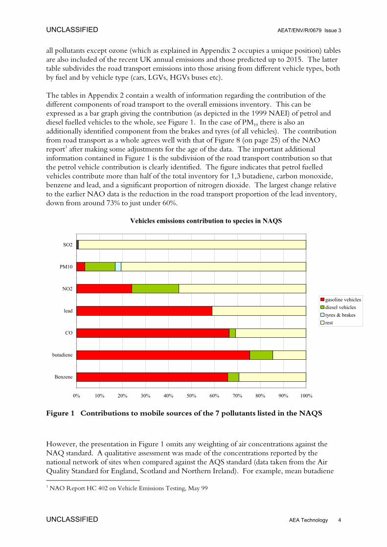
The tables in Appendix 2 contain a wealth of information regarding the contribution of thedifferent components of road transport to the overall emissions inventory. This can beexpressed as a bar graph giving the contribution (as depicted in the 1999 NAEI) of petrol anddiesel fuelled vehicles to the whole, see Figure 1. In the case of PM10 there is also anadditionally identified component from the brakes and tyres (of all vehicles). The contributionfrom road transport as a whole agrees well with that of Figure 8 (on page 25) of the NAOreport1 after making some adjustments for the age of the data. The important additionalinformation contained in Figure 1 is the subdivision of the road transport contribution so thatthe petrol vehicle contribution is clearly identified. The figure indicates that petrol fuelledvehicles contribute more than half of the total inventory for 1,3 butadiene, carbon monoxide,benzene and lead, and a significant proportion of nitrogen dioxide. The largest change relativeto the earlier NAO data is the reduction in the road transport proportion of the lead inventory,down from around 73% to just under 60%.
Figure 1 Contributions to mobile sources of the 7 pollutants listed in the NAQS
However, the presentation in Figure 1 omits any weighting of air concentrations against theNAQ standard. A qualitative assessment was made of the concentrations reported by thenational network of sites when compared against the AQS standard (data taken from the AirQuality Standard for England, Scotland and Northern Ireland). For example, mean butadiene 1 NAO Report HC 402 on Vehicle Emissions Testing, May 99
Vehicles emissions contribution to species in NAQS
0% 10% 20% 30% 40% 50% 60% 70% 80% 90% 100%
Benzene
butadiene
CO
lead
NO2
PM10
SO2
gasoline vehiclesdiesel vehiclestyres & brakesrest

UNCLASSIFIED AEAT/ENV/R/0679 Issue 3
UNCLASSIFIED AEA Technology 5
concentrations are around 40% of the 2.25 µg/m3 standard, with one of the thirteen monitoringsites being just above the standard (at 2.34 µg/m3) in the context of a decreasing inventory. Incontrast, nearly half of the 83 national monitoring sites exceeded the target annual mean NO2
concentration of 40 µg/m3, with concentrations generally being highest at roadside and kerbsidesites. A “mean” concentration of 120% of the AQS was taken for this pollutant. However, thesituation is more complex than this because for NO2 there are both hourly, and annual means.Further, with the latest revision the standard for the hourly mean has been reduced from 150ppb to 105 ppb (the standards for the annual mean has remained unaltered).
Figure 2 shows the previous data modified to include this weighting. All but two of thepollutants have an inventory less than 100, i.e. less than that required to meet the AQSStandards. The two pollutants that need further reducing are NO2 and PM10. Further, thecontribution of petrol vehicles to the overall NO2 inventory is significant.
Figure 2 Contributions to mobile sources of 7 pollutants listed in the AQS weightedby air concentrations relative to the AQS
2.1.3 Future trends
NO2 concentrations currently exceed the AQS standard, as discussed above. There are anumber of steps being taken to reduce these, not least in terms of the lowering of emission levelsfrom vehicles, and the effective policing of these changes to type approval standards. Nochange is expected in terms of the species specified in the AQS over the next decade, i.e. it isexpected to remain as NO2.
The situation is not as simple for particulate matter. This is currently the subject of intensiveresearch, and the complexity of the generic term is becoming apparent. The Air Quality
0
20
40
60
80
100
120
140
% of National target
Benzene butadiene CO lead NO2 PM10 SO2
Schematic of pollutant sources and extent
gasoline vehiclesdiesel vehiclestyres & brakesrest

UNCLASSIFIED AEAT/ENV/R/0679 Issue 3
UNCLASSIFIED AEA Technology 6
Strategy does not complicate the issue of particulate matter by giving any data for size rangesother than PM10. Such data can be obtained from the National Atmospheric EmissionsInventory directly2. Table 1 lists the UK emissions of various PM fractions in each sector in thePM10 inventory. The data is from the 1998 inventory, and for each size range is expressed interms of % of the whole, with the total mass in the size range, in k tonnes also being included.
Table 1 UK emissions for various PM size ranges
PM10 PM2.5 PM1.0 PM0.1
Combustion in energy production 19% 17% 14% 16%Combustion in comm/inst/residential 19% 16% 18% 7%Combustion in industry 10% 10% 7% 9%Production processes 22% 16% 12% 3%Road transport
Diesel combustion 17% 26% 33% 49%Petrol combustion 4% 7% 9% 12%Tyre & brake wear 3% 2% 1% 1%
Other transport 2% 3% 4% 2%Waste treatment & disposal 1% 1% 1% 1%TOTAL (k tonnes/year) 163 100 74 30
The message from this table is that whilst combustion processes in road transport are animportant contribution to the PM10 inventory, they become increasingly more important forsmaller size fractions. Consequently, any move to regulate or set standards for smaller sizefractions will lead to further pressure on road transport. It is noted that the principal contributoris the diesel fuelled fraction of the fleet which provides around 80% of the PM generated byroad transport combustion for all size ranges.
It is concluded that in anticipation of future trends in terms of the pollutants specified and likelystandards, an in-service test for petrol vehicles should aim to confirm that the emissions of CO,hydrocarbons (thence 1,3 butadiene and benzene) and NOX remain acceptable. Recentchanges in fuel specification mean that lead is no longer an issue. In contrast, because of itsimportance to air quality and possible changes in the metrics used, it is appropriate that thisproject consider the options for particulate measurement, specifically related to petrol vehiclesthat may be burning lubricating oil.
2 National Atmospheric Emissions Inventory: UK Emissions of Air Pollutants 1970 – 1998, Taken for the web site:http://www.aeat.co.uk/netcen/airqual/naei/annreport/annrep98/chap4_2.html.

UNCLASSIFIED AEAT/ENV/R/0679 Issue 3
UNCLASSIFIED AEA Technology 7
2.2 AN OVERVIEW OF THE NATIONAL ATMOSPHERICEMISSIONS INVENTORY AND THE CONTRIBUTION OF MOBILESOURCES.
2.2.1 Introduction
This section of the report considers the National Atmospheric Emissions Inventory (NAEI)from road transport emissions, and the assumptions that are used to forecast future emissions. Itis important to this project because it is the standard reference air emissions inventory for theUK and includes emission estimates for a wide range of important pollutants. This includesseven of the eight pollutants listed in the AQS, and for all the species specified in the typeapproval regulations (assuming road vehicle PM is equivalent to PM10, and “hydrocarbons” areequivalent to non-methane volatile organic compounds). The NAEI was used to generate theinventory data discussed in the previous section. It also is the basis upon which the effectivenessof various in-service testing scenarios are quantified, to give the reduction in emissions in unitsof mass/year, and their context in terms of the overall emissions inventory.
The objective of the NAEI with regard to road transport is to quantify:
.,emittedpollutantofmass yearainjourneysallvehiclesall∑∑
In practice this has to be achieved using a model. The fundamental methodology involves thecombining of vehicle emission factors with traffic activity and fleet composition data. The fleetcomposition is subdivided into six broad classifications: cars, LGVs, rigid HGVs, articulatedHGVs, buses and motor cycles. The first two of these are then further subdivided according tothe type of fuel its engine runs on; petrol or diesel. Each of the eight resulting classifications isthen further subdivided into different emissions standards as defined by successive EC directives,except the motor cycles, for which different regulations apply (Directives 97/24/EC and2000/51/EC).
A single average emissions factor (expressed in grams of pollutant per kilometre driven) can beproduced for each vehicle type and emissions class at each average speed for vehicles operatingat their normal operating temperature. The total emissions for the pollutants NOX, CO,benzene, 1,3-butadiene, methane, N2O, PM10 and non-methane volatile hydrocarbons(NMVOCs) are then, to a first approximation, calculated by multiplying the emissions factorsby the number of vehicle kilometres for each vehicle type and road type and summing.
The basic assumptions and methodology that are pertinent to this study on petrol fuelledvehicles and were used for the 1998 NAEI road transport emission projections are summarisedin Appendix 3.
The model incorporates assumptions, often as sub-models, to take account of• the degradation in emissions as vehicles age,• the additional emissions that arise from vehicles when they start from cold and• evaporative emissions from vehicles.
One aspect of particular significance to this project is that of “cold start emissions”. These whenexpressed as a fraction of the urban inventory from petrol fuelled vehicles, were calculated to be:

UNCLASSIFIED AEAT/ENV/R/0679 Issue 3
UNCLASSIFIED AEA Technology 8
• NOX 15.8 %• PM10 12.8%• CO 54.1 %• NMVOCs 26.9 %
i.e. contribute a significant proportion of the inventory.
2.2.2 The use of this model in this project
It can be assumed when assessing the effectiveness of various in-service emissions testing regimesthat these will only affect the emissions factors (the mass of pollutants emitted per km driven).Therefore it is assumed that different in-service testing scenarios will have no impact on the fleetcomposition, or the traffic activity. Consequently, when quantifying the effectiveness of variousin-service emissions testing regimes, the parameter that will be varied is the emission factors, togive a revised inventory, and therefore by subtraction from the base cases tabulated in Appendix3B net changes in pollutant mass emitted per year can be computed.
It is also noted that the NAEI model used in this study is the same model that was used by theCleaner Vehicle Task Force in its analysis.

UNCLASSIFIED AEAT/ENV/R/0679 Issue 3
UNCLASSIFIED AEA Technology 9
3 Modelling the distribution ofexhaust emissions
Key issues addressed in Chapter 3
The primary objective of this chapter is to develop a relevant mathematical model. This isachieved by:• considering models that may be appropriate• assessing the suitability of the available data sources• developing a mathematical model of the distribution of exhaust emissions in the fleet,• fitting it to pre-existing emissions data
3.1 INTRODUCTION
The purpose of this section of the study is to:1. establish the emissions performance of the fleet2. estimate the number of catalyst equipped vehicles which are above the new vehicle emissions values
(accounting for scatter on new vehicle emissions figures)3. estimate the distribution of the excess emissions from these vehicles, e.g. what percentage of them are
more than 25%, 50%, 100%, 200% etc above the new vehicle emissions level(Italics are used to identify phrases taken verbatim from the Customer’s ITT.)
This information is a precursor to• quantifying the effect of different levels of degradation on the AQS targets,• identifying the reasons for excessive emissions• evaluating the effectiveness of the current in-service test at identifying the excess emitters• quantifying the “savings potential”, and hence the cost effectiveness that a revised test might
deliver• providing some indications as to the proportion of the savings potential that revised tests
might achieve.
It is appreciated that reality is not so simple.
3.2 APPROACH FOR QUANTIFYING WHAT VEHICLES AREEMITTING – DEVELOPMENT OF A MATHEMATICAL MODEL
The ITT states: It is envisaged that this task will require the development of a mathematical model whichwill need to take account of:• the amount and proportion of the vehicle fleet whose emission performance has degraded,• the impact of failing vehicles on National Air Quality Strategy objectives.

UNCLASSIFIED AEAT/ENV/R/0679 Issue 3
UNCLASSIFIED AEA Technology 10
Therefore, the approach adopted in this project is to use existing data to check/construct amathematical model and then to use the model as the principal predictive tool. Further data, ordata collection exercises would then be used initially to confirm the validity of the model andthen to refine key parameters.
Despite extensive searching the author has been unable to find a validated model, or acceptedmethodology, in the literature. Therefore such a model is developed here.
Some desirable characteristics of the model are:• it is statistically validated,• the number of variables subsumed within it is as small as possible, i.e. it is a simple as
practicable, and• the variables can be related to physical observables, rather than abstract constants.
The following distributions were compared with the data available:1. binomial distribution2. multinomial and χ2 distributions3. normal distribution4. Poisson distribution.
None of these common distribution functions provides a good representation of the realdistributions. The principal mismatch occurs because of the asymmetric shape of the real data.
3.2.1 Log normal distributions
A distribution profile that is much closer, providing a good fit for many data, is the log normaldistribution. This can be described as the normal distribution plotted on a logarithmic abscissa.
In a normal distribution the fraction of the whole population (δN/N) with values of property xbetween x and x+δx is given by:
( )x
xNN
δ
σµ−
−σπ
=δ
2
2
2exp
21
where µ = the arithmetic mean value of x in the whole population, andσ is a constant, the standard deviation of the population from the mean.
This distribution is often seen in a simplified form where the mean value, µ, is zero to give theformula for a gaussian error curve which is symmetric about the y-axis.
−
π=φ
2exp
21 2x
(x)
In the log normal distribution x is replaced by log(x), to give

UNCLASSIFIED AEAT/ENV/R/0679 Issue 3
UNCLASSIFIED AEA Technology 11
( )
σµ−
−σπ
=φ 2
2
2)exp
21 (xlog
x)(log
Figures 3 and 4 show illustrative graphs of this function, with µ = 1.0 and σ = 1.5. In Figure 3the value of x is plotted on a linear axis, whilst in Figure 4 it is plotted on a logarithmic axis,demonstrating the function’s relationship with a gaussian. The axes of both graphs are labelledemissions in g/km, and fraction of the population because these units are relevant to this study.
Figure 3 Graph of log normal function, with µ = 1.0 and σ = 1.5 plotted on a linearaxis
Figure 4 Graph of log normal function, with µ = 1.0 and σ = 1.5 plotted on alogarithmic axis
0
0.05
0.1
0.15
0.2
0.25
0.3
0.35
0 20 40 60 80 100 120 140
Value of x on a linear scale (e.g. emissions in g/km)
φ(lo
g x)
0
0.05
0.1
0.15
0.2
0.25
0.3
0.35
0.01 0.1 1 10 100 1000
Value of x on a logarithmic scale (e.g. emissions in g/km)
φ(lo
g x)

UNCLASSIFIED AEAT/ENV/R/0679 Issue 3
UNCLASSIFIED AEA Technology 12
Having defined a distribution function using the log-normal model, the data can be furthermanipulated. For each emissions level (g/km) given the fraction of the population emitting atthis level, the emissions from this fraction of the population is the product of the two. Theseproducts can be summed to give an accumulating value of emissions, which can be expressed asa percentage of the whole. When this parameter is plotted against the emissions level (in g/km),a graph as illustrated in Figure 5 is formed. The EU Joint Commission study (JCS) presentedsome of its data in this form, see for example Figure 7 reproduced from the JCS Main Report.
Figure 5 Accumulating value of emissions plotted against emission levels
The fraction of the population emitting at a particular level can also be summed and expressed asa percentage of the whole population. When the cumulative emissions (as a %) is plotted againstthis parameter a graph as illustrated in Figure 6 results. The JCS study presented some of its datain this form also, see also Figure 7 reproduced from the JCS Main Report.
Figure 6 Cumulative emissions plotted against the fraction of the populationemitting at a particular level
0
10
20
30
40
50
60
70
80
90
100
0 20 40 60 80 100 120 140
Emissions g/km
% o
f tot
al e
mis
sion
s
0
10
20
30
40
50
60
70
80
90
100
0 10 20 30 40 50 60 70 80 90 100
Cumulative vehicle number (%)
% o
f tot
al e
mis
sion
s

UNCLASSIFIED AEAT/ENV/R/0679 Issue 3
UNCLASSIFIED AEA Technology 13
Fitting the model to experimentally determined data is the reverse of the process described. Itrequires the experimental data to be digitised, e.g. data in the format of either Figures 5 or 6,and then superimposing calculated data. The values of the model’s two parameters (the meanand standard deviation) are then varied such that a best fit is obtained. This fitting can beachieved using a least squares fitting algorithm or by eye. The latter is useful if it is found thatno ideal fit can be obtained and one wishes to use one’s judgement to define the “best fit”. Inthis work both approaches were used.
3.3 REVIEW OF DATA SOURCES AVAILABLE
This section reviews the available datasets against which to fit the model.
In general there are three types of source data that are available, and a fourth that might beavailable, that might be appropriate for this study. These are:• the JCS study on in-use car I&M,• the DTLR’s rolling programme of emissions factor generation for the NAEI,• the German in-use compliance programme• various other in-use compliance programmes both within Europe and in the US.
The two principal criteria on which the potential quality of data can be judged are the drivecycles over which it was collected and the size and method of selection of the vehicles sampled.
3.3.1 The JCS study on in-use car I&M
This study was funded by three of the European Commission’s Directorate Generals (DG VII,XI and XVII). It title, the inspection of in-use cars in order to attain minimum emissions of pollutantsand optimum energy efficiency describes its principal objectives. A range of cars were tested, whichincluded 192 cars fitted with TWCs. Testing was undertaken principally during 1995 – 1997.
Two distinct sample populations were tested. The first was known as the Random (JCSnomenclature) sample and comprised 135 vehicles that were offered for testing by owners.(The owners would have been aware of why the testing organisations wished to borrow theirvehicles.) The JCS study comments “despite the fact that the sample is considered as random, ithas to be stressed that there is a certain bias, due to the voluntary participation in the testprogramme; in general, owners of well maintained cars are suspected to have a higherwillingness to participate in such tests.
The second sample population is referred to as the Total sample and comprised the 135 vehiclefrom the random sample plus a further 57 vehicles selected from vehicle groups where highemitters can be expected, e.g. high mileage vehicles and high emitters as detected by remotesensing (of CO, HC and NO). These additional 57 vehicles were acknowledged to haveunrepresentatively poor emissions performance.
Therefore the emissions distribution of a truly representative sample probably lies somewhere inbetween the emission distribution of the two sample groups.

UNCLASSIFIED AEAT/ENV/R/0679 Issue 3
UNCLASSIFIED AEA Technology 14
All vehicles were tested over a number of long cycles, including the NEDC, and a range ofshort cycles, including the current two speed idle test. The results from the latter tests arediscussed in the next chapter. The data is attractive for this study because:• it contains emissions over the NEDC• it is reasonably contemporary• the sample size is moderately large, and• the method of sample selection has been carefully considered such that two data sets exist,
most probably bracketing the emissions performance of the fleet as a whole.
3.3.2 The DTLR’s rolling programme of emissions factor generation
The latest batch of data from this programme has kindly been supplied by DTLR’s VSE2Division.
The latest set of data was obtained from 5 vehicles, 2 diesel and 3 petrol (with TWCs) fuelledvehicles. Not only is this sample small, but it is believed to be unrepresentative because the verypurpose of testing these vehicles (to obtain emission factors for the NAEI model) means that apoorly maintained excess emitter would be rejected as inappropriate for testing.
The data collected was for steady state driving, i.e. hot start, driving at 90 and 113 km/hr,evaluating the effects of:• ambient temperature – vehicles were tested at –7°C, 7°C and 25°C;• running on standard and low sulphur fuel; and• turning the air conditioning on at 25°C ambient temperature.
Whilst these data are valuable for developing the model for which they were collected, they arenot relevant to defining the distribution of emissions performance of the fleet as a whole overthe type approval regulatory cold start cycle.
3.3.3 The German in-use compliance programme
The objective of this programme is to establish whether or not the emissions performance of“new” vehicles remains within EU defined limits of the revised type approval standard as theyaccumulate miles; the in-service compliance aspect of the directive. Importantly, it is theemissions of vehicles maintained according to the manufacturers specifications that are assessedas part of the enlarged type approval specification, as detailed in directive 98/69/EC (anamendment to directive 70/220/EEC).
AEA Technology has been provided with a report on in-use compliance testing by the UBA3.This report, which is in German, contains information on 34 vehicles, taken from 10 specificmodels. The vehicles were tested over both the relevant type approval drive cycle(ECE+EUDC) and the in-service two speed idle test. Emissions data is presented for eachvehicle. None of the vehicles had high (more than twice) the type approval emissions standard,although several were outside the in-use compliance standards. The author is not aware of the
3 Report kindly supplied by W Niederle, UBA, report issued by RWTÜV, author Helge Smidt, 14 February 2001,in German.

UNCLASSIFIED AEAT/ENV/R/0679 Issue 3
UNCLASSIFIED AEA Technology 15
details of the vehicle selection procedure, however, as noted earlier what should be tested areappropriately maintained vehicles.
The above German in-use compliance data can be compared with the data from the JCS study.For the latter 60% of the cumulative CO emissions from the “Total” sample were generated bythe worst 10% of the sample, and it is recognised that the emissions from the “Total” sample arepoorer than would be expected from the fleet as a whole. The former studied only 34appropriately maintained vehicles. Given that it would probably be inaccurate to describe theworst 10% of vehicles in the fleet as appropriately maintained and the size of the sample, it is nottoo surprising that no high excess emitters were found in the German study. However, anotherplausible hypothesis that is not eliminated by these data is that generally levels of emissionsdegradation have reduced between the two studies.
Overall, it is felt that the data in the UBA report is generally consistent with the JCS findings. Itis acknowledged that the sample size is significantly smaller, and that the degree of maintenanceis above average. Consequently, this data was not used as the basis for fitting the model.
3.3.4 Other in-use compliance programmes
Summary information from the Swedish in-use compliance assessment programme has beenforwarded by DTLR’s VSE2 Division. This is much more extensive than the German data,containing emissions results for around 100 different models, which involved testing around 450vehicles.
The data available to date, however, is of average emissions for each model. This smoothes outindividual very high emitters, reducing the extreme value by around a factor of 3 to 6(dependent on the number of vehicles of that model that were tested). The comments made inthe previous section regarding the selection of vehicles for the German in-use complianceprogramme apply equally here – it is very likely that the vehicles tested were “above average”with regards to their level of maintenance, and below average with regards to their emissions.
These data were not fitted to the distributions.
3.4 MODELLING OF THE JCS DATA
In this section the log normal distribution model, as described in Section 3.2 will be fitted to theJCS data. The key data in the JCS Main Report are contained in Figures 13 to 15 of the JCSreport, where data from both the “Total” and “Random” groups are given before and aftermaintenance. These figures are reproduced as Figure 7 of this report to aid the reader. The dataare presented as percentage cumulative emissions against cumulative vehicle number (expressedas a percentage) and percentage of total emissions against emissions in g/km. The predictionsfrom the model can be manipulated to generate data in this form.

UNCLASSIFIED AEAT/ENV/R/0679 Issue 3
UNCLASSIFIED AEA Technology 16
Figure 7 Figures 13, 14 and 15 of the JCS Study main report

UNCLASSIFIED AEAT/ENV/R/0679 Issue 3
UNCLASSIFIED AEA Technology 17
3.4.1 Oxides of nitrogen
Figure 8 shows a fit of the model to the JCS experimental data for the “Total” sample. Thevalues of the mean and standard deviation parameters within the model are given in Table 2.Also included in the table is an indication of the error for the parameters. This was obtainedsemi-quantitatively by noting the range of values for the parameters before the fit deterioratedfrom good to moderate (as judged by eye).
Figure 8 Fitting of the model to the JCS NOX data
Figure 8a, Percentage of total NOX emissions for cumulative vehicle number
0
10
20
30
40
50
60
70
80
90
100
0 10 20 30 40 50 60 70 80 90 100
Cumulative vehicle number (%)
% o
f tot
al N
OX e
miss
ions
Model predictionsJCS NOx data
Figure 8b, Percentage of total NOX emissions against vehicular emission rate
0
10
20
30
40
50
60
70
80
90
100
0 0.5 1 1.5 2 2.5
NOX emissions g/km
% o
f tot
al N
OX e
miss
ions
Model predictionsJCS NOx data

UNCLASSIFIED AEAT/ENV/R/0679 Issue 3
UNCLASSIFIED AEA Technology 18
Table 2 Parameters used in the log normal model to reproduce the JCS data
mean standard deviationOxides of nitrogen 0.192 ± 0.01 g/km 1.05 ± 0.05Hydrocarbons 0.22 ± 0.03 g/km 1.0 ± 0.1Carbon monoxide – “Total” sampleCarbon monoxide – “Random” sample
2.7 ± 0.2 g/km2.7 ± 0.2 g/km
1.5 ± 0.20.95 ± 0.05
Carbon dioxide 183 ± 5 g/km 0.30 ± 0.03
From Figures 13 and 14 of the JCS report it is seen that for NOX there was little differencebetween the emissions distributions from the “Total” and “Random” samples and therefore asingle set of parameters for the model reproduced the emissions from both samples. Similarly,from JCS Figure 15 it is apparent that maintenance of the “gross polluters” led to little change inNOX emissions (around 5% and selectively for only the very worst emitters. Both theseobservations imply that NOX emissions, like CO2 emissions, are affected only very little by thestate of maintenance of the vehicle.
3.4.2 Hydrocarbons
The experimentally determined emissions from both the “Total” and “Random” samples areplotted in Figure 9 together with a fit using the model. Parameters were selected for the modelthat gave a distribution profile intermediate between the two sample groups, and these are givenin Table 2.
Figure 9a, Percentage of total hydrocarbons emissions for cumulative vehicle number
0
10
20
30
40
50
60
70
80
90
100
0 10 20 30 40 50 60 70 80 90 100
Cumulative vehicle number (%)
% o
f tot
al H
C e
mis
sion
s
Model predictionsJCS HC from "Total" sampleJCS HC from "Random" sample
UNCLASSIFIED AEAT/ENV/R/0679 Issue 3
UNCLASSIFIED AEA Technology 19
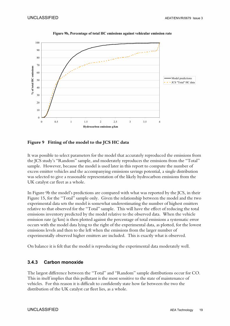
Figure 9 Fitting of the model to the JCS HC data
It was possible to select parameters for the model that accurately reproduced the emissions fromthe JCS study’s “Random” sample, and moderately reproduces the emissions from the “Total”sample. However, because the model is used later in this report to compute the number ofexcess emitter vehicles and the accompanying emissions savings potential, a single distributionwas selected to give a reasonable representation of the likely hydrocarbon emissions from theUK catalyst car fleet as a whole.
In Figure 9b the model’s predictions are compared with what was reported by the JCS, in theirFigure 15, for the “Total” sample only. Given the relationship between the model and the twoexperimental data sets the model is somewhat underestimating the number of highest emittersrelative to that observed for the “Total” sample. This will have the effect of reducing the totalemissions inventory predicted by the model relative to the observed data. When the vehicleemission rate (g/km) is then plotted against the percentage of total emissions a systematic erroroccurs with the model data lying to the right of the experimental data, as plotted, for the lowestemissions levels and then to the left when the emissions from the larger number ofexperimentally observed higher emitters are included. This is exactly what is observed.
On balance it is felt that the model is reproducing the experimental data moderately well.
3.4.3 Carbon monoxide
The largest difference between the “Total” and “Random” sample distributions occur for CO.This in itself implies that this pollutant is the most sensitive to the state of maintenance ofvehicles. For this reason it is difficult to confidently state how far between the two thedistribution of the UK catalyst car fleet lies, as a whole.
Figure 9b, Percentage of total HC emissions against vehicular emission rate
0
10
20
30
40
50
60
70
80
90
100
0 0.5 1 1.5 2 2.5 3 3.5 4
Hydrocarbon emissions g/km
% o
f tot
al H
C e
mis
sion
s
Model predictionsJCS "Total" HC data

UNCLASSIFIED AEAT/ENV/R/0679 Issue 3
UNCLASSIFIED AEA Technology 20
Figure 10 shows the two experimentally determined distributions together with a model for thedata that lies some where between the two. The values for the model’s parameters are given inTable 2. Generally the fit can be at best described as moderate.
A fit to just the “Random” sample’s data is also shown in Figure 10a. This was obtained bymerely varying the standard deviation parameter, i.e. keeping the mean emissions rate constant.In this case the fit can be described as good. The model’s predictions compared with theemission distribution when plotted against % of total emissions, Figure 10b, is moderate to poor.The same systematic variations that applied to the modelling of the hydrocarbons data also applyto, and are observed with, this data.
These two distributions should be regarded as a lower limit for the number of excess emitters(the “Random” sample) and a more likely, but possibly high, limit of the number of excessemitters. When evaluating the cost effectiveness of an in-service scheme, see Chapter 7, boththese distributions are used to provide a measure of the uncertainty involved when computingthe CO emissions savings potential.
The good agreement between the model’s predictions and the “Random” sample indicates thatthis sample can be accurately described by a log normal distribution function. However, thegenerally only moderate agreement between the model’s predictions and the “Total” sample’sCO emissions indicates this is not the case for the “Total” sample. This most probably arisesbecause the selection methodology for the “Total” sample leads to a high fraction of very highemitters, more than is in the fleet as a whole, and more than the simple log normal distributionpredicts. Further, because the data in the JCS study reports are always presented usingcumulative emissions, or percent of total emissions, this high fraction of very high emittersdistorts the scaling of the y-axis. This distortion, in turn, further emphasises the difference.
Figure 10a, Percentage of total CO emissions for cumulative vehicle number
0
10
20
30
40
50
60
70
80
90
100
0 20 40 60 80 100
Cumulative vehicle number (%)
% o
f tot
al C
O e
mis
sion
s
Model predictionsJCS CO from "Total" SampleJCS CO from "Random" SampleModel predictions - Fit to random sample

UNCLASSIFIED AEAT/ENV/R/0679 Issue 3
UNCLASSIFIED AEA Technology 21
Figure 10 Fitting of the model to the JCS CO data
Overall, it is felt that the model is providing a useful descriptive tool for the data reported in theJCS study. Consequently, it is a potentially useful predictive tool, with the quality of fit toexperimental data providing an estimate of the robustness of quantitative predictions.
3.4.4 Carbon dioxide
The JCS CO2 data was also fitted to the model, although this parameter is not directly relevantto this study. The details are given in Appendix 4. It is interesting to note that for this atypicalcomponent of the exhaust emissions good agreement between the model and experimental datawas obtained.
3.4.5 Summary of modelling
A log normal model has been applied and was found to be a moderate to good fit to the dataobtained from the JCS study depending on the pollutant. For carbon monoxide the JCS datashowed a large difference between the “Total” and “Random” samples. It is believed that thedistribution of emissions from the whole fleet lies somewhere between the two JCSdistributions.
Figure 10b, Percentage of total CO emissions against vehicular emission rate
0
10
20
30
40
50
60
70
80
90
100
0 10 20 30 40 50 60 70 80 90 100
Emissions g/km
% o
f tot
al C
O e
mis
sion
s
Model predictionsJCS "Total" CO data

UNCLASSIFIED AEAT/ENV/R/0679 Issue 3
UNCLASSIFIED AEA Technology 22
4 Definition of an “excess emittervehicle and significance of vehicleswith deteriorated emissionperformance
Key issues addressed in Chapter 4
This chapter builds on the mathematical model developed in the previous one. Its primaryfocus is to derive a definition for the excess emitter vehicles and to assess the importance ofthese to the emissions inventory by using the model to calculate the emissions from the excessemitters. This augmented by considering the degradation mechanisms that lead to a vehiclebecoming an excess emitter.
4.1 DEFINITION OF AN EXCESS EMITTER
The principal parameter when quantifying the degradation of emissions performance is thechange in what vehicles actually emit into the environment and its impact on human health andthe environment.
Regulatory emissions measurements, made on an elderly vehicle fitted with closed loop fuellingcontrol and a TWC, illustrate some of the complexities involved. The vehicle had travelledaround 125,000 miles (200,000 km), and was approved to 91/441/EEC. Emissions weremeasured with the vehicle in three configurations:1. with a new replacement catalyst fitted2. with the vehicle fitted with its original catalyst, and3. with an empty catalyst casing replacing the catalyst.The vehicle was tested over three different drive cycles:a. a directive 98/69/EC defined type approval cycle (the NEDC),b. the NEDC cycle but with the vehicle started when its oil temperature was already at its
operating temperature, i.e. around 85°C, instead of soaked for at least 12 hours at ambienttemperature as in test a), and
c. at a steady 120 kph, when all temperatures were stable.
The CO, HC and NOX emissions are given in Table 3.

UNCLASSIFIED AEAT/ENV/R/0679 Issue 3
UNCLASSIFIED AEA Technology 23
Table 3 Emissions of vehicle with variable catalytic activity over various drive cycles
Cold start NEDCall emissions expressed as g/km CO THC NOX
Vehicle fitted with New catalyst 2.827 0.303 0.089Vehicle fitted with Original catalyst 4.638 0.315 0.224Vehicle fitted with No catalyst 8.646 0.519 1.261
Hot start NEDCall emissions expressed as g/km CO THC NOX
Vehicle fitted with New catalyst 0.206 0.013 0.075Vehicle fitted with Original catalyst 2.038 0.086 0.195Vehicle fitted with No catalyst 7.115 0.534 1.192
Hot steady 120 kphall emissions expressed as g/km CO THC NOX
Vehicle fitted with New catalyst 0.018 0.01 0.063Vehicle fitted with Original catalyst 0.062 0.01 0.104Vehicle fitted with No catalyst 6.107 0.332 3.213
MOT emission measurementsNormal idle speed Fast idle speed
CO(%)
THC(ppm)
CO(%)
THC(ppm)
Lambda
Vehicle fitted with New catalyst 0.002 7 0.001 6 1.005Vehicle fitted with Original catalyst 0.005 16 0.174 15 1.010Vehicle fitted with No catalyst 0.534 63 0.495 24 1.000
An in depth analysis of these data is not appropriate but some comments pertinent to the currentproject illustrate some important issues. The data are of interest because they are a series ofcontrolled experiments where two parameters are varied: catalyst activity and the test cycles. Interms of the vehicle catalysts the brand new and no catalyst are two extremes with the originalcatalyst intermediate between these.
For the new catalyst the cold start NEDC gives significant CO and hydrocarbon emissionsbecause of the over-fuelling required for cold starting, see Section 2.2.1 and the catalyst not upto its operating temperature. In contrast, the hot start NEDC give much lower emissions ofboth because no over-fuelling occurs, and because the catalyst operates effectively from the startof the cycle. Similarly, 120 kph steady state driving leads to very low emissions.
For the original (an aged) catalyst, the CO and hydrocarbon emissions caused by over-fuellingare expected to be the same as when the new catalyst was fitted (it being the same vehicle). Theadditional emissions arise from the longer time it takes the original catalyst to reach atemperature at which it converts virtually all CO to CO2. This phenomenon is seen again overthe hot start NEDC cycle, where the emissions for the vehicle fitted with the original catalystarise principally from the time it takes for the catalyst to reach a temperature where it oxidisesthe CO, the new catalyst doing this virtually from the start of the cycle.
In contrast, at a steady 120 kph, both catalysts give negligible CO, hydrocarbons or NOX
emissions, especially with respect to when no catalyst was fitted. This is because under these

UNCLASSIFIED AEAT/ENV/R/0679 Issue 3
UNCLASSIFIED AEA Technology 24
conditions both the new and original catalyst are at a sufficiently high temperature (knowncolloquially as the “light-off temperature” or “being lit”) to efficiently destroy the pollutantspresent. Therefore despite the large volumes of exhaust gas being produced, emission values arelow. Whilst the data presented here are for 120 kph steady state driving, data at idle, 30 kph, 70kph and 90 kph follows this trend also.
The data for the MOT test, the unloaded engine at normal or fast idle, also follows the patternof both catalysts giving similar emissions, especially with respect to when no catalyst was fitted.
To summarise, the reduction in catalyst efficiency is only apparent at intermediate “conditions”:When the catalyst is either cold or very hot its activity is very similar to that of a new catalyst.
The findings that low idle, high idle and 120 kph measurements do not show large changesbetween the new and old catalysts, but the cold, or hot, start NEDC does demonstrate animportant shortcoming of the current in-service test, and provide guidance on how it might beimproved:• steady state testing under no load is not effective at monitoring catalyst activity, and• making the catalyst work harder by testing under load at a steady state is also ineffective at
evaluating catalyst activity.
It must be emphasised that what is being stated here is that the current test is very poor atassessing catalytic activity. However, loss of catalytic activity is only one of several faults thatcause changes in emissions, see Section 4.2.2. Further, the current in-service test is found to bebetter at identifying the majority of other faults, see the table at the end of Section 5.3.6. It isthis ability to detect other faults that leads to the assessment that the current test is performingmoderately, and is providing a positive contribution to improving air quality.
From Table 3 the type approval test cycle when the vehicle was fitted with a new catalyst gaveemissions that met the limit values specified in directive 94/12/EC (after making due allowancefor the change in test cycle, which the Vehicle Certification Agency give as being 30%), seebelow:
Table 4 Limit values for emissions from passenger cars as specified in directives94/12/EC and 98/69/EC Stage A
CO HC NOX HC+NOX
94/12/EC standard for ECE+EUDC 2.2 g/km 0.5 g/kmInferred 94/12/EC standard over NEDC 3.28 g/km 0.5 g/km98/69/EC Stage A standard for NEDC 2.3 g/km 0.2 g/km 0.15 g/km 0.35 g/km
From this we can conclude that in terms of emissions the vehicle was well maintained andrunning close to its specification. When compared to the emissions measured when no catalystwas fitted, it is also apparent that for all pollutants the catalyst is having an advantageous effect.
The performance of a catalyst can be expressed in a number of ways: e.g. as a change in theemissions, in absolute terms, relative to some standard, or as a percentage of its effect relative totheir being no catalyst present.

UNCLASSIFIED AEAT/ENV/R/0679 Issue 3
UNCLASSIFIED AEA Technology 25
If E1, E2 and E3 denote the emissions of a pollutant from the vehicle for the configurations 1 to 3listed above, then two measures of performance are:• performance of old catalyst relative to a new catalyst = E2/E1
• performance of old catalyst relative to a no catalyst = E2/E3.
The first definition is usually adopted with E1 being an emissions standard.
Over the 98/69/EC defined type approval cycle (NEDC) the CO emissions of the vehiclewhen fitted with the original catalyst are 1.64 times the CO emissions from when the vehicle isfitted with a new catalyst, i.e. the aged catalyst has caused emissions to increase by 64%.However, for the hot start NEDC test the original catalyst leads to 9.9 times the CO emissionsfrom the new catalyst, an 890% increase. As explained earlier this is attributed to the originalcatalyst requiring some time to reach its operating temperature, whereas the new catalystconverted efficiently from the start of the test. At the steady speed of 120 kph CO emissionsshow a 245% increase.
If the effect of the original catalyst is expressed as a percentage of the total emissions (measuredwhen no catalyst was fitted), then it consumes:
for the type approval test 46.4% of CO emissionsfor the hot start NEDC test 71.4% of CO emissions, andat a steady 120 kph 99.0% of CO emissions.
On the basis of this information is this vehicle, when fitted with its original catalyst anexcess emitter?
Whilst the answer should be a simple yes or no, one would be forgiven for saying yes inresponse to some data and no in response to other data. The variable rates of emissionsdegradation for different drive cycles are an important, fundamental finding. This impactson both the definition of an excess emitter, and the efficacy of different testing procedures atidentifying them.
The definition of an excess emitter adopted by this project is to use that embodied in the “in-service compliance” portion of the amending EC directive 98/69/EC to directive70/220/EEC. Some reasons/justification for this adoption include:• it is building on the collective wisdom of many interested parties• it is the “accepted” degradation rate used within the EU• it is based on absolute emissions, measured in g/km, contributing directly to the nation’s
atmospheric emissions inventory, and• it is measured over a cold start loaded cycle, simulating some urban driving where the
impact of emissions on air quality to human health is most sensitive.
Therefore, a vehicle is an excess emitter if its CO, HC or NOX emissions are outsidethose of the European standard that applies when measured over the 98/69/ECspecified type approval drive cycle (the NEDC) after due allowance has been madefor degradation at the rate of an additional 20% for each 50,000 miles (80,000 km) thatthe vehicle has been driven.
This is exactly equivalent to the 1.20 degradation factor for all three regulated pollutants that iswritten into directive 98/69/EC.

UNCLASSIFIED AEAT/ENV/R/0679 Issue 3
UNCLASSIFIED AEA Technology 26
On this basis, for the vehicle tested because it had travelled 200,000 km, the degradation factorto apply is an additional 50% (20% x 200/80) to the revised 94/12/EC limit values standardsgiven in Table II of the directive. This gives:
CO HC NOX HC+NOX
Inferred 94/12/EC limit values for NEDC 3.28 g/km 0.5 g/kmInferred 94/12/EC limit values+ 50% degradation 4.875 g/km 0.75 g/kmActual emissions 4.64 g/km 0.32 g/km 0.22 g/km 0.54 g/km
On this basis the vehicle when fitted with its original catalyst and tested over the NEDC, thisvehicle is not an excess emitter! However, if the vehicle were assessed over a hot startNEDC relative to the performance of a new catalyst it would be viewed as an excess emitter.The explanation for this being that on a hot start test a new catalyst very rapidly reaches atemperature at which it efficiently oxidises CO, whereas the old catalyst is slower to do so.
There is a further issue involved in deciding whether or not an individual vehicle is an excessemitter. This arises because the EC directives consider a vehicle type as a whole. (Initially asingle “representative” vehicle of each type is tested before an approval is issued. The CoP andin-service compliance testing use statistical sampling, once vehicles are in production, todemonstrate compliance. This testing is conducted by the manufacturer and the results areaudited by the approval authority.) Consequently, only a small fraction of the vehiclesproduced are tested and not all the vehicles tested have to meet the limits, merely a sufficientlyhigh proportion have to be sufficiently below the limit. In contrast, in-service testing considerseach vehicle individually. Consequently, it is possible for a brand new vehicle of a make that istype approved, to never meet the type approval limit values. If the in-service test exactlymatched these limit values this vehicle would, therefore, fail in its “showroom” condition.Exactly the same dilemma occurs when defining an excess emitter because, like the in-servicetest, individual vehicles, rather than the ensemble, are measured against limit values.
4.1.1 Calculation of the number of excess emitters in the fleet
In the previous chapter we have defined the basis for a mathematical model of the fleet’semissions distribution (Section 3.2), and fitted the model to the JCS study’s data (Section 3.4).In the first section of this chapter we have derived a definition for an excess emitter. These arenow to be combined such that the model is used to calculate the number of excess emitters.However, whilst it is the model that is used for these calculations, the model’s parameters arethose chosen that gave a good fit to the JCS data. Consequently, the data from the JSC study,though not being used directly, is intimately linked to the results obtained.
It is noted that the majority of vehicles tested in the JCS study complied with directive91/441/EEC, rather than the more recent 94/12/EC directive. This is not too surprising giventhe dates the two standards were introduced and the date of the study. Therefore the “standardthat applies” in the definition will be taken as that specified by directive 91/441/EEC.
The limit values given in the directive 91/441/EEC for the ECE + EUDC test are (see inAppendix 1):

UNCLASSIFIED AEAT/ENV/R/0679 Issue 3
UNCLASSIFIED AEA Technology 27
CO 2.72 g/km HC + NOX 0.97 g/km.
What is required in order to relate these data to JCS study data is the equivalent limit values fordirective 91/441/EEC over the NEDC.
Considering CO first: it is generally accepted that 98/69/EC CO limit value over the NEDCrepresents a 30% reduction over the 94/12/EC limit.Given the former is 2.3 g/km CO, then the latter is simply:
CO/km.g 3.28 i.e. 30 - 100
100 2.3 NEDC over valueslimit 94/12/EC ×=
The 91/441/EEC and 94/12/EC CO limit values are 2.72 and 2.2 g CO/km, respectively.
g/km. 4.06 i.e. CO/km,g 3.28 2.202.72
NEDC the over valuelimit CO 91/441/EEC the Therefore ×=
Moving on to consider hydrocarbons and NOX:for 98/69/EC Stage A and B the ratio of HC:NOX is 56.5%:43.5%.
Using this same proportion the 0.97 g/km HC + NOX 91/441/EEC limit values are sub-divided into 0.55 g/km HC and 0.42 g/km NOX.
The reduction in HC and NOX limit values between directives 94/12/EC and 98/69/EC StageA appear more severe, since there is a reduction of 30% (from 0.50 to 0.35 g/km for the sum ofthe two) before any difference in the effect of changing the drive cycle is included. It was seenthat the 30% reduction for the CO standard is predominantly due to the change in drive cycleand the sensitivity of CO emissions to cold start conditions. In section 2.2.1 the contributionsof cold emissions, expressed as a fraction of the urban inventory were calculated to be:
NOX 15.8% CO 54.1% and NMVOCs 26.9%.
A pro rata scaling of the 30% cold start contribution for CO on going from the ECE+EUDC tothe NEDC gives the following cold start contributions:
NOX +9% CO +30% and NMVOCs +15%.
These figures are taken as the reduction in emissions caused by changing the drive cycle, and arecompounded with the change given in g/km. Thus the 91/441/EC limit value for theECE+EUDC standard need to be increased by these amounts, i.e.
g/km. 0.46 i.e. 9 - 100
100 0.42 NEDC over valueslimit NO 91/441/EC
and g/km, 0.65 i.e. 15 - 100
100 0.55 NEDC over valueslimit NMVOC 91/441/EC
X ×=
×=
Finally, the definition of an excess emitter requires that allowance be made for degradation inemissions performance caused by the distance the vehicle has travelled. From Table 5 withinthe JCS Detailed Report 3, it is found that for the “Total” sample the average distance travelled
UNCLASSIFIED AEAT/ENV/R/0679 Issue 3
UNCLASSIFIED AEA Technology 28
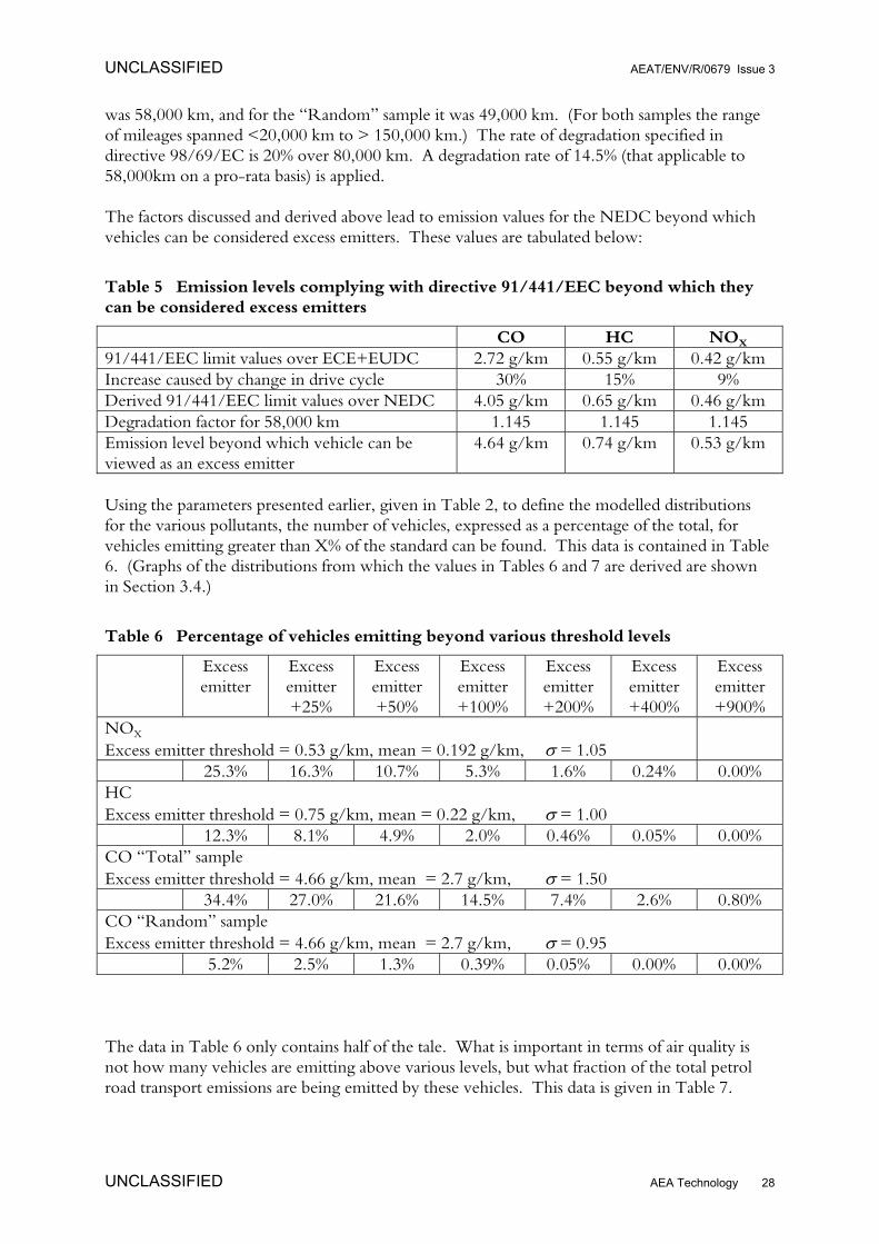
was 58,000 km, and for the “Random” sample it was 49,000 km. (For both samples the rangeof mileages spanned <20,000 km to > 150,000 km.) The rate of degradation specified indirective 98/69/EC is 20% over 80,000 km. A degradation rate of 14.5% (that applicable to58,000km on a pro-rata basis) is applied.
The factors discussed and derived above lead to emission values for the NEDC beyond whichvehicles can be considered excess emitters. These values are tabulated below:
Table 5 Emission levels complying with directive 91/441/EEC beyond which theycan be considered excess emitters
CO HC NOX
91/441/EEC limit values over ECE+EUDC 2.72 g/km 0.55 g/km 0.42 g/kmIncrease caused by change in drive cycle 30% 15% 9%Derived 91/441/EEC limit values over NEDC 4.05 g/km 0.65 g/km 0.46 g/kmDegradation factor for 58,000 km 1.145 1.145 1.145Emission level beyond which vehicle can beviewed as an excess emitter
4.64 g/km 0.74 g/km 0.53 g/km
Using the parameters presented earlier, given in Table 2, to define the modelled distributionsfor the various pollutants, the number of vehicles, expressed as a percentage of the total, forvehicles emitting greater than X% of the standard can be found. This data is contained in Table6. (Graphs of the distributions from which the values in Tables 6 and 7 are derived are shownin Section 3.4.)
Table 6 Percentage of vehicles emitting beyond various threshold levels
Excessemitter
Excessemitter+25%
Excessemitter+50%
Excessemitter+100%
Excessemitter+200%
Excessemitter+400%
Excessemitter+900%
NOX
Excess emitter threshold = 0.53 g/km, mean = 0.192 g/km, σ = 1.0525.3% 16.3% 10.7% 5.3% 1.6% 0.24% 0.00%
HCExcess emitter threshold = 0.75 g/km, mean = 0.22 g/km, σ = 1.00
12.3% 8.1% 4.9% 2.0% 0.46% 0.05% 0.00%CO “Total” sampleExcess emitter threshold = 4.66 g/km, mean = 2.7 g/km, σ = 1.50
34.4% 27.0% 21.6% 14.5% 7.4% 2.6% 0.80%CO “Random” sampleExcess emitter threshold = 4.66 g/km, mean = 2.7 g/km, σ = 0.95
5.2% 2.5% 1.3% 0.39% 0.05% 0.00% 0.00%
The data in Table 6 only contains half of the tale. What is important in terms of air quality isnot how many vehicles are emitting above various levels, but what fraction of the total petrolroad transport emissions are being emitted by these vehicles. This data is given in Table 7.

UNCLASSIFIED AEAT/ENV/R/0679 Issue 3
UNCLASSIFIED AEA Technology 29
Table 7 Percentage of total emissions generated by vehicles emitting beyond variousthreshold levels
Excessemitter
Excessemitter+25%
Excessemitter+50%
Excessemitter+100%
Excessemitter+200%
Excessemitter+400%
Excessemitter+900%
NOX
Excess emitter threshold = 0.53 g/km, mean = 0.192 g/km, σ = 1.0552.9% 40.4% 30.9% 19.2% 8.1% 1.9% 0.1%
HCExcess emitter threshold = 0.75 g/km, mean = 0.22 g/km, σ = 1.00
35.9% 24.6% 17.4% 9.1% 2.9% 0.5% 0.0%CO “Total” sampleExcess emitter threshold = 4.66 g/km, mean = 2.7 g/km, σ = 1.50
74.2% 67.0% 60.4% 50.7% 34.6% 18.8% 5.8%CO “Random” sampleExcess emitter threshold = 4.66 g/km, mean = 2.7 g/km, σ = 0.95
16.8% 9.8% 5.9% 2.3% 0.5% 0.04% 0.00%
Some observations on these data are:• for NOX a somewhat surprisingly high number of vehicles generate emissions above the
standard, and this gives rise to a high associated fraction of total emissions;• for NOX, where the model fits the JCS data well, the figures are very close to those seen in
Figure 15 of the JCS Main Report; i.e. around 50% of total emissions coming from vehiclesemitting >0.5 g/km and around 20% from vehicles emitting >1.0 g/km;
• for HC the percentages are smaller than for NOX; i.e. around 40% of total emissions comingfrom vehicles emitting >0.75 g/km, the standard for HC;
• for CO there are large differences between the data for the “Random” and “Total” samples;• for the “Random” sample only 5.2% of vehicles emitted more than the 4.66 g/km standard,
contributing 16.8% of the emissions;• the point above agrees with the JCS data, see Figure 14 of the JCS Main Report, i.e. Figure
7 of this report;• for the “Total” sample, the model indicates 34.4% of vehicles emit more than 4.66 g/km
CO, and now contribute around 75% of the emissions;• the point above agrees with the JCS data, see Figure 13 of the JCS Main Report, i.e. Figure
7 of this report;• from Figure 15 of the JCS Main Report, around 30% of the cumulative emissions come
from vehicles emitting >50 g/km CO, whereas the model predicts only 5.8% withemissions more than 47 g/km, i.e. the model underestimates the number of the very highestemitters.
4.1.1.1 NOX performance:The data for NOX emissions are something of an enigma. The model reproduces the JCS datawell, i.e. the model’s predictions and the JCS data are in good agreement. Both find(surprisingly?) high numbers of vehicles emitting above the NOX standard. Even if the standardwas incorrect, and the figure used was the same as for HCs, the percentage of vehicles emittingbeyond the standard, and their contribution to the total emissions, would have been similar to

UNCLASSIFIED AEAT/ENV/R/0679 Issue 3
UNCLASSIFIED AEA Technology 30
those for HCs, i.e. around 12% of vehicles contributing around 35% of the total emissions.What is more notable is that the fraction of excess emitters appear independent of the sample(with the distributions of the “Random” and “Total” samples being virtually identical). Inaddition the emissions performance is very resistant to maintenance, with the maintainedvehicles performing in a nearly identical manner to samples pre-maintenance.
Given the importance of vehicular NOX emissions to the meeting of Air Quality standards, thereasons for the above observations require further study, with appropriate remedial strategies tobe identified. This should be undertaken in Phase 2 of the project.
4.1.1.2 CO performance:The second notable aspect of this analysis is how the range of excess emissions predicted for COis very dependent on sample selection/vehicle maintenance. The two sets of model parameterschosen might be taken as bracketing the real situation. However, it is noted that the modelpredictions for the “Total” sample, is still a significant underestimation of the emissions fromvehicles emitting greater than ten times the standard. The percentages of total emissionsgenerated by vehicles beyond the standards are 74.2% and 16.8% for the “Total” and“Random” groups modelled, respectively. However this presentation of data somewhat hidesthe nature of the excess emissions because there is an inverse proportionality involved. This isbecause:
.cemaintentan after fleet from Emissions
maintaince after fleet from Emissions-emaintenanc before fleet from Emissionsemissions Excess =
It will be seen in Chapter 7, where savings potentials are calculated, that the savings potential forthese two scenarios are approximately 300% and 23% respectively.
For this pollutant we have the opposite effect noted for NOX, namely that the emissionspotential is very dependent on vehicle sample or state of maintenance. Therefore, theintroduction of a perturbation to current practice, e.g. E-OBD, could change the emissionsdistribution, and consequently the savings potential. This too will be considered further inPhase 2 of the project.
4.2 ASSESSMENT OF LIKELY DEGRADATION MECHANISMS
4.2.1 Overview of TWC vehicle technology
Modern petrol fuelled vehicles are very far removed from vehicles of two decades ago.Consequently, there has been a major change in the degradation mechanisms that lead tochanges in the vehicles’ emissions. It is therefore useful to briefly review the technologyinvolved.
Internal combustion engines consume air and fuel to generate useful mechanical work, heat andemissions. An extremely valuable parameter characterising the combustion mixture is the ratioof the quantity of air supplied relative to the theoretical requirement to obtain total oxidationof the fuel supplied. This parameter is known as lambda (λ). When the quantity of air suppliedis equal to the theoretical requirement λ=1.00, a lean mixture (λ>1) contains excess air, and a
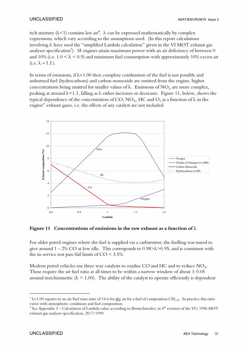
UNCLASSIFIED AEAT/ENV/R/0679 Issue 3
UNCLASSIFIED AEA Technology 31
rich mixture (λ<1) contains less air4. λ can be expressed mathematically by complexexpressions, which vary according to the assumptions used. (In this report calculationsinvolving λ have used the “simplified Lambda calculation” given in the VI MOT exhaust gasanalyser specification5). SI engines attain maximum power with an air deficiency of between 0and 10% (i.e. 1.0 < λ < 0.9) and minimum fuel consumption with approximately 10% excess air(i.e. λ = 1.1).
In terms of emissions, if λ<1.00 then complete combustion of the fuel is not possible andunburned fuel (hydrocarbons) and carbon monoxide are emitted from the engine, higherconcentrations being emitted for smaller values of λ. Emissions of NOX are more complex,peaking at around λ=1.1, falling as λ either increases or decreases. Figure 11, below, shows thetypical dependence of the concentration of CO, NOX, HC and O2 as a function of λ in theengine'’ exhaust gases, i.e. the effects of any catalyst are not included.
Figure 11 Concentrations of emissions in the raw exhaust as a function of λ
For older petrol engines where the fuel is supplied via a carburettor, the fuelling was tuned togive around 1 – 2% CO at low idle. This corresponds to 0.98>λ>0.95, and is consistent withthe in-service test pass/fail limits of CO < 3.5%.
Modern petrol vehicles use three way catalysts to oxidise CO and HC and to reduce NOX.These require the air fuel ratio at all times to be within a narrow window of about ± 0.05around stoichiometric (λ = 1.00). The ability of the catalyst to operate efficiently is dependent
4 λ=1.00 equates to an air/fuel mass ratio of 14.6 for dry air for a fuel of composition CH1.85. In practice this ratiovaries with atmospheric conditions and fuel composition.5 See Appendix 3 – Calculation of Lambda value according to Brettschneider, in 4th revision of the VI’s 1996 MOTexhaust gas analyser specification, 20/7/1999.
0
2
4
6
8
10
12
14
0.8 0.9 1 1.1 1.2
Lambda
Exh
aust
com
posi
tion
(%)
OxygenOxides of Nitrogen (x1,000)Carbon MonoxideHydrocarbons (x100)
CO
HC
NOx
Oxygen

UNCLASSIFIED AEAT/ENV/R/0679 Issue 3
UNCLASSIFIED AEA Technology 32
on it maintaining a sufficient oxygen storage capacity (often known as the OSC) and theengine’s control system providing both the correct range of lambda and at the right frequency.
Most modern vehicles are fitted with an array of sensors. These include, for example, enginetemperature sensors, an inlet air mass flow meter and a manifold depression sensor. There is alsothe accelerator pedal, whose position is sensed. The outputs of these, and other sensors, are fedinto the electronic control unit (ECU) and are used to define which map, and which point onit, should be used to define the quantity of fuel injected and its timing. However, the ECU isprogrammed to learn, and to update the map with “modified” values that ensure λ is kept in thecorrect range. Further, if a sensor were to fail, the ECU would detect this and use aconservatively pre-set default value, or default engine control maps. The ECU would alsoilluminate a warning lamp on the dash-board. This might be an engine management warninglight, or for a car with emissions on-board diagnostics (E-OBD) the malfunction indicator light(MIL).
4.2.2 Faults that cause changes in emissions
For a correctly operating vehicle with closed loop fuelling control and a three way catalyst thereare far fewer faults that lead to excess emissions than on older petrol cars. The following“single” faults, however, do lead to excess emissions:failure of the closed loop fuelling system
• lambda-sensor fault• electrical fault associated with the lambda-sensor (e.g. earthing, connector
separating or a wiring fault)• ECU fault• injector failure• engine temperature sensor• failure to move beyond the “warm up” phase into closed loop control (e.g. caused
by a faulty engine temperature sensor)• air fuel meter
failure of the catalyst• loss of catalytic activity• loss of mechanical integrity such that some of the exhaust gas can bypass the active
elementleakage in the exhaust system between the engine and the catalyst.
In addition to the primary faults above, there are a number of other faults which could affectemissions performance in a less serious manner by causing the engine’s management system torevert to “default” values or engine maps rather than fine tuning the fuelling quantity andtiming to the actual conditions. For a vehicle operating in closed loop fuelling mode, thesefaults are, to a large extent, self-rectifying. These faults include failure of the:
• fuel trim value sensor• misfire sensor• knock sensor• air intake temperature sensor

UNCLASSIFIED AEAT/ENV/R/0679 Issue 3
UNCLASSIFIED AEA Technology 33
• intake manifold air pressure sensor• throttle position sensor• idle speed actuator• air mass flow sensor• coolant temperature sensor• oil temperature sensor• engine speed sensor• camshaft position sensor• EGR valve sensor• secondary air injection pump• E-OBD MIL light bulb.
4.2.3 Detection of faults and rates of failure
The question: “what are the rates of failure for the different faults listed in the previous section”is actually profound! Unless something is deliberately measured or checked, or unless it causesan undesirable effect (e.g. the vehicle can not be driven, or it uses large additional quantities offuel) changes will pass unnoticed.
For the vast majority of vehicle owners the inspection and maintenance and self policing theyundertake is:• the statutory annual roadworthiness test (for vehicles > 3 years old)• sufficient repair to enable continued use of the vehicle, and• an annual service.

UNCLASSIFIED AEAT/ENV/R/0679 Issue 3
UNCLASSIFIED AEA Technology 34
The faults listed above can be analysed in terms of their visibility to, or impact on, these threechecks:
Fault MOT Vehicle stopper Annual serviceFailure of closed loop controlλ-sensor fault 50% probability rarely possible if check
engine light onelectrical fault from λ orother critical sensors
50% probability possible possible if checkengine light on
ECU fault possible – rarely getsto this stage
probable possible – rarely getsto this stage
Failure of catalystloss of catalytic activity not unless extremely
severeno no
loss of mechanical integrity yes if >20% leakage no nocorrosion etc yes – c.f. exhaust
leakagerarely yes – c.f. exhaust
leakageleakage in exhaust system yes – checked rarely
An interesting aspect of the above analysis is that catalytic activity is not really assessed in anytest. (Catalytic activity can be described as the ability of the catalyst to convert gaseouspollutants into acceptable gaseous emissions.) The fast idle emissions component of the MOTtest is undertaken on a hot engine, with a hot catalyst using relatively low gas flows and COlevels. Therefore, apart from virtually a catastrophic loss of activity, high conversion rateswould be seen provided that the exhaust gas’s stoichiometry was correct, i.e. the close loopfuelling system was operating correctly.
In terms of quantifying the rates of degradation, the most thorough data is provided in a TRLreport entitled “An analysis of data from the MOT test”6. In this report data on how vehiclesfail was found from three sources:• garages• road-side callout data from the RAC, and• leasing companies.Information was also provided by a company that manufactures replacement exhaust andcatalyst systems.
Data from garagesThree garages were selected, two were main dealers (Audi/VW and Ford) and the other“specialised” in MOT testing. Over around a four month period 523 MOT tests werereported, of these there were 11 failures (2.1%).
Three of the failures occurred at the main dealers. Two failed on high λ for the fast idle test.Rectification comprised mending an electrical connection between the λ sensor and the ECUfor one vehicle and replacing the exhaust system for the other vehicle. The third failure wasdue to high CO at fast idle, where the heated exhaust gas oxygen (i.e. λ) sensor was found to befaulty. 6 “An analysis of data from the MOT test”, TJ Barlow, RS Bartlett and ICP Simmons, TRL Project reportPR/SE/474/98, September 1998.

UNCLASSIFIED AEAT/ENV/R/0679 Issue 3
UNCLASSIFIED AEA Technology 35
The other eight MOT failures were at the non-main dealer garage, and faultfinding and repairwas not undertaken at that garage. Hence no further information was forthcoming about thesevehicles.
Statistically this sample is very small, and care should be exercised when trying to project thesefindings to the parc as a whole.
Roadside callout dataThe RAC provided TRL with data on breakdowns for the years 1995, 1996 and 1997. Aroundthree million incidents were recorded for each year. Faults are categorised by a three digit code,and TRL extracted those they felt were related to emissions as:
• ECU engine management• wiring loom – engine management• catalytic converter• air flow sensors• throttle sensors• manifold pressure sensors• oxygen/λ sensors.
Based on this assumption, the following data were extracted:
1995 1996 1997Fault No of
incidences% of allfaults
No ofincidences
% of allfaults
No ofincidences
% of allfaults
ECU enginemanagement
6,349 0.21 6,564 0.20 8,404 0.27
Wiring loom –enginemanagement
3,001 0.10 3,157 0.10 2,971 0.10
Catalyticconverter
764 0.03 1,124 0.03 1,284 0.04
Air flow sensors 1,204 0.04 1,403 0.04 1,252 0.04Throttle sensors 1,007 0.03 1,241 0.04 1,001 0.03Manifold pressuresensors
271 0.01 285 0.01 320 0.01
Oxygen/λ sensors 226 0.01 310 0.01 300 0.01
Total emissionfaults
12,822 0.43 14,084 0.44 15,533 0.50
The majority of callouts are for faults which prevent the vehicle from either starting orcontinuing a journey, vis:
flat battery 6.0% of all incidencesdefective battery 4.9% of all incidenceswheel change 3.54% of all incidences, etc.
Most emissions based faults are not actually vehicle stoppers – they may cause an “engine fault”light to become illuminated, and the driver requests help to check whether it is sensible to

UNCLASSIFIED AEAT/ENV/R/0679 Issue 3
UNCLASSIFIED AEA Technology 36
continue the journey or start the car. The author also questions TRL’s inclusion of all enginemanagement and wiring faults, and throttle sensor faults. The majority of faults classified ineither of the first two are most likely to be for sub-systems other than those related to emissions.Similarly, if the throttle sensor stops working the vehicle will probably stop, having lost a crucialcontrol signal, but the emissions will probably be unaffected. Consequently, the author believesthe 0.43 – 0.50% total of all callouts is an overestimate by a factor of 2 to 4, i.e. only 0.12 – 0.25of all callouts are emissions related.
It is again emphasised that these figures are not the totality of the frequency of failures of theemissions system because many failures neither prevent the vehicle from starting nor cause arunning vehicle to stop.
Data from lease companiesTRL obtained data from a major leasing company that owns around 71,000 vehicles. Theyprovided data on vehicles that had their catalysts replaced in 1997. There were 105 replacementcatalysts fitted, with the average distance driven per failure as 69,300 miles (111,500 km).
A summary of the catalyst failure modes was given, classified into:Damaged Noisy Leaks Worn Contaminated Corroded Defective
5 1 2 5 2 12 78
These findings have been discussed, in general terms, among a number of automotive engineers.Broadly they were sceptical regarding what “defective” covered, particularly in the context of itbeing 75% of the catalyst failures, and the necessity of replacing all the catalysts that werereplaced. For example, if a repairer experiences difficulty in removing a failed λ sensor from thecan he might “opt” for a total catalyst replacement even though the catalyst was still sufficientlyactive.
TRL comment that the average failure rate of a catalyst per 69,300 miles is significantly abovethe 150,000 mile lifetime “claimed” (although there is no further explanation of the origins ofthe 150,000 miles expected life). However, it is likely that closer scrutiny might reveal that thisis a pessimistically biased figure.
A second major leasing company also supplied data covering its passenger car fleet of about60,000 vehicles. Table 8 shows the failure rates for emissions related components that theyrecorded.

UNCLASSIFIED AEAT/ENV/R/0679 Issue 3
UNCLASSIFIED AEA Technology 37
Table 8 Failure rates for emissions related components
Component Number of failures Failure rate (per million km)Catalyst 286 0.15λ sensor 153 0.08Idle valve 135 0.07Exhaust manifold 132 0.07Ignition coil 103 0.05Ignition ECU 95 0.05Crankshaft sensor 79 0.04Distributor 68 0.04Map sensor 33 0.02Throttle switch 33 0.02Fuel system ECU 17 0.01Cambelt 7,855 4.09The sum of the faults tabulated above, ignoring the cambelt, is 0.60 faults per million km. Thecambelt is included because it is also present in the RAC data, where it accounted for 1.64% ofall callouts. Using the factor 0.4 to “convert” the lease hire data (failure rate / million km) withthe RAC data (fraction of total callouts), this lease hire data would predict a callout proportionof 0.24% (0.60 × 0.4). Therefore, whilst it is accepted that this data is quite old, it is for 1994, itis consistent with the RAC data.
Data from catalyst and replacement exhaust manufacturerTRL also approached catalyst and replacement exhaust manufacturers. Information wasreceived from one exhaust manufacturer, who gave the following approximate breakdown ofthe reasons for catalyst failure:
• 90% of replacements are due to the ceramic monolith breaking up;• a further 5% are due to the failure of supporting pipe-work or brackets, necessitating a
replacement part, and• the remaining 5% are due to a fault in the closed loop management system damaging the
monolith, again resulting in a new replacement being fitted after rectification of the fault.
Poisoning through the use of leaded fuel, unusual drive cycle or crash impact damage are alsoreasons for failure, but these were not thought to be significant.
Some likely causes for ceramic monolith break-up are:• mechanical shock sustained because of rough terrain, poor driving style or human
intervention,• thermal shock sustained by cold water dowsing/enveloping the catalyst,• poor catalyst design or manufacture resulting in the thermal blanket/monolith support
system yielding and allowing monolith movement and subsequent self destruction,• incorrect tuning of the engine or malfunction of an engine management component
resulting in continued high temperature operation beyond the monoliths normal range,• poor engine design leading to poor combustion efficiency or over-fuelling producing
continued high temperature operation beyond the monoliths normal range.

UNCLASSIFIED AEAT/ENV/R/0679 Issue 3
UNCLASSIFIED AEA Technology 38
The implementation from October 1999 of the EC Directive which prohibits the sale of non-type approved catalysts should cause the frequency of the third item on the list to becomenegligible.
4.2.4 Concluding summary
Overall, the major faults that cause deterioration in emissions performance have been listed. Interms of the real frequency of failure there are serious difficulties in gathering unbiased,objective, statistically meaningful data.
For some faults like catalyst activity, none of the three routes whereby faults are usuallyidentified will detect other than a major failure. Specifically, the current in-service test is noteffective at detecting low catalyst activity and consequently catalyst failure is not being detectedand rectified as frequently as might be required.
The general consensus for the frequency of faults influencing emissions is, in descending order:• λ sensor faults• catalyst internal integrity• catalyst external integrity (corrosion or other leaks)• others.

UNCLASSIFIED AEAT/ENV/R/0679 Issue 3
UNCLASSIFIED AEA Technology 39
5 Effectiveness of current annual testat identifying “excess emitters”
Key issues addressed in Chapter 5
Given that Chapter 4 concludes that the UK’s vehicle fleet does contain excess emittingvehicles whose emissions contributions are adversely affecting air quality, the study moves onto consider the effectiveness of the current annual emissions test. This is accomplished byanswering the following questions.• What are the criteria for the success of an in-service test?• What is the current in-service test procedure?• What is the effectiveness of the current test from an assessment or reanalysis of data from
previous studies?
5.1 SUCCESS CRITERIA
The criteria for the success of an in-service test are not simply the percentage of target vehiclesdetected; they are more complex. In this report they are assumed to be:• to maximise the likelihood of detecting the worst offenders, i.e. to maximise the reduction
in emissions, and• to minimise the number of vehicles erroneously labelled as requiring maintenance.
Pass
/fail
limit
Emission standard
Emis
sion
s ove
r Typ
e A
ppro
val c
ycle
Emissions over in-service test
Area 1 Area 2
Area 3 Area 4
Errors of omission
Errors of commissionAppropriate passes
Appropriate failsInappropriate passes, i.e.
Inappropriate fails, i.e.

UNCLASSIFIED AEAT/ENV/R/0679 Issue 3
UNCLASSIFIED AEA Technology 40
This can be explained pictorially in the manner used, for example, in the JCS study. In theillustration above, the emissions of a vehicle over the type approval cycle are plotted against theemissions measured by an in-service short test. A horizontal line is drawn perpendicular to the“real” emissions axis at the standard. A vertical line denotes the pass/fail limit for the short test.The resulting four areas are:area 1 vehicles whose “real” emissions are below the standard and are correctly identified
as passes by the in-service test.area 2 vehicles whose “real” emissions are below the standard but are identified as fails by
the in-service test. These are known as the errors of commissionarea 3 vehicles whose “real” emissions are above the standard but are identified as passes
by the in-service test. These are known as errors of omissionarea 4 vehicles whose “real” emissions are above the standard and are correctly identified
as fails by the in-service test.
The objective of the in-service test is to maximise the proportion of vehicles in area 4 and tominimise the proportion of vehicles in area 2. Further, given a non-ideal test, and given therewill be some vehicles in area 3, the pass/fail threshold should be optimised in such a way so as tomaximise the emissions savings made, i.e. if the in-service test fails to detect some vehiclesemitting above the emissions standard, these vehicles should be those that are only just over thestandard.
5.2 CURRENT TEST PROCEDURE FOR VEHICLES WITH SIENGINES AND A TWC
Information on the current test procedure to be applied to vehicles was taken from the VIpublication “In-service exhaust emission standards for road vehicles, 7th Edition.
5.2.1 Visual inspection
Once the preliminary checks have been completed, the tester will raise the engine speed totypically 2,500 rev/min, or half the maximum engine speed if this is lower. The engine speedwill be held steady for about 20 seconds then the engine will be allowed to return to its naturalidle speed. Once the emissions have stabilised the tester will assess the smoke emitted from thetailpipe. If the vehicle is emitting dense blue or clearly visible black smoke then the vehicle willfail the test.
5.2.2 Catalyst test procedure
For vehicles subject to this procedure the emissions are assessed during two separate tests. Thefirst test consists of checking the emissions at “high-idle” which involves running the engine atthe speed specified in the Annex to the VI’s in-service exhaust emission standards for roadvehicles publication, typically 2,500 – 3,000 rev/min over a 30 second period. During this highidle the analyser automatically checks the emissions of CO and HC and a check is made on theλ value (limits also listed in the VI standards publication). Provided that the results are equal to

UNCLASSIFIED AEAT/ENV/R/0679 Issue 3
UNCLASSIFIED AEA Technology 41
or below the specified limits, the vehicle will have passed this section of the test and the analyserautomatically proceeds to the standard idle test.
Whilst there is some variability in the emissions limits for the high idle test, as discussed in depthin Section 6.4, standard/default values are:
CO ≤ 0.3%HC ≤ 200 ppm (as calibrated with propane, i.e. C3 equivalent)0.97 ≤ λ ≤ 1.03.
The standard idle test is carried out with the engine at its normal idling speed and the analyserdisplays the results continuously. Once a stabilised figure is achieved, the analyser records theCO value only and compares it with the value from the VI standards publication. There issome variability in this emissions limits. The standard/default value is:
CO ≤ 0.5%.
Because the extended emissions test (used for vehicle fitted with catalysts) is more complicatedthan a single engine speed test (used for pre-catalyst vehicles) the emissions analysers aredesigned to a more stringent standard and include menu driven computer software designed toguide the tester through the test sequence. The analyser requires the tester to complete eachstage of the test before proceeding to the next. In addition, where a failure is recorded duringthe high idle test then the analyser automatically schedules a repeat test. This is to ensure, as faras practical, that the catalytic converter has reached its normal operating temperature.
Before starting the emissions test the tester will check the engine oil temperature to ensure thatthe engine is at the manufacturer’s stated operating temperature. This requires a temperatureprobe to be inserted into the dipstick tube.
In the event of a vehicle failing the high idle test but passing the low idle test, the analyserautomatically sequences a period of “preconditioning” followed by a further high idle test. Thevehicle must pass both the high idle test and the standard idle test to secure a pass result.
5.2.3 Basic emissions test (BET)
In order to reduce testing time, improve convenience and answer some of the criticisms madein the NAO report, the VI have introduced a voluntary fast track test for vehicles registered onor after 1/8/92. This came into effect from 1/9/01. Its basic philosophy is to check a vehicleagainst generic levels. If the vehicle is within these limits then the vehicle has passed, and nofurther testing is required. If the vehicle does not meet these limits it is not failed but testedusing the longer test, described in Section 5.2.2. The use of generic limits obviates the need tofind, and enter into the test equipment, the vehicles engine number thereby circumventing oneof the principal difficulties encountered by testers.
The test involves ensuring the engine is hot enough to test, e.g. by inspecting the vehicle’scoolant temperature sensor, checking it has hot coolant hoses or noting that the coolant fan hascut in. (This removes the need to insert a thermocouple into the engine’s sump, via the dipstickport to measure engine temperature.) The fast idle test is then conducted with the enginerunning at between 2500 and 3000 rev/min. The criteria for a pass are that for the raw exhaust

UNCLASSIFIED AEAT/ENV/R/0679 Issue 3
UNCLASSIFIED AEA Technology 42
CO and HC concentrations should be below, and λ should be between, the standard/defaultvalues listed in the previous section.
The engine is then tested at normal idle, which is required to meet the relatively generous limitsof being between 450 and 1500 rev/min. The criteria for a pass are that for the raw exhaust:• CO concentration <= 0.5% (rather than testing to manufacturer defined limits as is currently
done).
If the vehicle’s emissions comply with these generic limits then it passes the emissions test forthis roadworthiness inspection.
5.3 EFFECTIVENESS OF THE CURRENT TEST PROCEDURE
5.3.1 Assessment methodology
The success criteria given at the start of this section were concerned with correctly identifyingthe “excess emitter” vehicles and, at the same time, not failing vehicles whose emissionsperformance is satisfactory.
Section 4.1 defined the target vehicles, the excess emitters, as those outside the appropriateEuropean standard, after making allowances for degradation, when assessed over the standardtype approval cycles, the NEDC. Herein lies a challenge because most information on thecurrent in-service test does not have data on the type approval emissions. Therefore such datacan not be used to assess how effectively the excess emitters are being detected, or the extent towhich vehicles with satisfactory emissions are being incorrectly failed. However, such datadoes contain some relevant information regarding the current pass/fail rates, the principalreasons for failure and other insights into the current test which give indications regarding howit could be improved.
The data assessed here are:• the Joint Commission Study (JCS),• the Transport Research Laboratory’s (TRL’s) study,• the National Audit Office (NAO) report and• some recent studies undertaken by the VI.
5.3.2 Analysis of the findings from the JCS study
The Joint Commission Study (JCS) was entitled “The inspection of in-use cars in order to attainminimum emissions of pollutants and optimum energy efficiency”. As part of this studyvehicles were tested over the type approval cycle specified in directive 98/69/EC (NEDC), anumber of other loaded cycles and the in-service two speed idle test according to directive92/55/EEC. (This has now been subsumed into, and superseded by, more recentroadworthiness directives, i.e. directive 96/96/EC and its amending directives 1999/52/EC and2001/9/EC.) Therefore, although the number of vehicles tested in the JCS study is less than inthe TRL study, the JCS data is crucial because it also contains emission information from thesedifferent test cycles.

UNCLASSIFIED AEAT/ENV/R/0679 Issue 3
UNCLASSIFIED AEA Technology 43
In Chapter 3 of this report, the JCS data was used as the foundation for developing a model ofcurrent vehicle emissions for on-the-road driving. In this part of the study the vehicles areviewed as individual test platforms. They can be categorised as either excess or acceptableemitters, using the criteria established in the previous chapter, and the results from an in-servicetest can be correlated with this categorisation.
The researchers responsible for generating the JCS reports did this, and their comments andconclusions are relevant to this study. It must be remembered that the in-service test accordingto the directive differs slightly from that used in Britain in a few respects, namely:• HC emissions were not measured, merely CO and λ, and• the same pass/fail points were used for all vehicles (CO ≤ 0.5% for normal idle and at high
idle CO ≤ 0.3%, 0.97 ≤ λ ≤ 1.03) as opposed to the UK where vehicle specific limits areused except for high idle CO.
The JCS study evaluated 192 cars fitted with closed loop fuelling and TWC systems. 135 werein the “Random” group and a further 57 were selected as “likely high emitters”.
The JCS defined “high emitters” as vehicles emitting more than 50% above the type approvalstandard. This JCS definition of “high emitters” is more lax than the proposed “excess emitter”definition developed in this report. For the average 58,000 km travelled by the vehicles testedin the JCS study, those emitting 14.5% above the their type approval standard would be viewedas “excess emitters” by the definition given in Section 4.1. This is in contrast to the 50% excessrequired before the JCS study labelled a vehicle as being a “high emitter”.
Following testing the vehicles the JCS defined as “high emitters” were maintained and thenretested. The emissions before and after maintenance can be used to calculate an “EmissionReduction Rate Potential” (ERRP). ERRP is defined in the JCS study as7:ERRP for pollutant = 100 x excess emissions of vehicles identified as needing maintenance
cumulative emissions of pollutant from whole sample
where excess emissions = emissions before maintenance – emissions following maintenance.
This is exactly the parameter required to assess the effectiveness of an I&M regime.
The ERRPs for the “Total” (Random + High Emitters) and the “Random” samples werecalculated for each pollutant, and are shown in Figure 12. The number of vehicles correctlyidentified as requiring maintenance (labelled P6) and incorrectly identified as requiringmaintenance (labelled P2) are shown in Figure 13.
7 See Section 4.2 of JCS Detailed Report 5, by LAT/AUTh, published April 1998.

UNCLASSIFIED AEAT/ENV/R/0679 Issue 3
UNCLASSIFIED AEA Technology 44
Figure 12 The ERRPs for the “Total” and the “Random” samples
Figure 13 The number of vehicles correctly and incorrectly identified as requiringmaintenance
-10.0%
0.0%
10.0%
20.0%
30.0%
40.0%
50.0%
60.0%
CO CO2 HC NOx
ERR
P (%
) Idle "Total" sampleHigh idle "Total" sampleIdle "Random" sampleHigh idle "Random" sample
0.0%
2.0%
4.0%
6.0%
8.0%
10.0%
12.0%
14.0%
% of vehicles correctly identified as being excessemitters
% errors of commission
Num
ber
of v
ehic
les i
n ca
tego
ry a
s a p
erce
ntag
e of
the
who
le sa
mpl
e
Idle "Total" sampleHigh idle "Total" sampleIdle "Random" sampleHigh idle "Random" sample

UNCLASSIFIED AEAT/ENV/R/0679 Issue 3
UNCLASSIFIED AEA Technology 45
From the NEDC emissions the number of vehicles identified as requiring maintenance (i.e. thatwere more than 50% above the vehicles’ type approval standard) were 24 (18%) and 55 (29%)for the random and total samples, respectively. Given the number of vehicles correctlyidentified as requiring maintenance from the high idle test, see Figure 13, (3.9% and 12.7%, or 5and 24, respectively), the number of errors of omission (the difference between the number ofvehicles identified by the two speed idle test and the number that should have been identifiedrelative to the total sample size) are 19 and 31 vehicles for the random and total samples,respectively. For these samples the 2-speed idle test only successfully detected 21% and 44% ofthe “high emitters” in the random and total samples, respectively.
From these data the JCS researchers made the following remarks8: (It should be rememberedthat the JCS study assessed a range of short tests, i.e. less than the full type approval test, some ofwhich were loaded. The aspects of the study reviewed here concerns the results from theunloaded test as per directive 92/55/EEC.)
• The short test in question seems to be efficient enough when the vehicle sample comprises of many highpolluters (total sample). However, this environmental benefit is accompanied by a relatively largenumber of errors of commission especially when only vehicles emitting 50% above the standard is theobjective.
• When only the random vehicle sample is taken into account the environmental benefit becomesextremely small. This remark along with the fact that there are many errors of commission leads to theconclusion that this short test is completely ineffective when applied to TWC equipped vehicles, whichis representative to the vehicle fleet.
• The first partial test measuring CO at idle seems to have no effect on the short test when only therandomly chosen vehicles are selected. It detects very few vehicles and as a result the environmentalbenefit is extremely small.
• λ measurement is, as expected, capable of detecting vehicles emitting very high levels of NOX.However, it is the parameter principally responsible for the errors of commission. This is particularlyobvious when targeting only to polluters 50% above the standard. When targeting to all vehiclesemitting above the standard it can be stated that even though λ measurement adds approximately 3%errors of commission, it also contributes to environmental benefit (1% CO, 0.5% HC and 4.5%NOX) by detecting almost 3% of these excess emitters.
The validity of the above results and the fact that the randomly chosen vehicles are indeed representative ofthe vehicle fleet has been proved by comparing these results to those coming from RWTÜV9. According tothem 3.47% of vehicles have been detected as having emissions above the type approval standard, while inthe sample of this report the corresponding percentage is 8.73%. The difference is attributed to the fact thatthe RWTÜV data is from an official inspection programme and as a result the owners have their vehiclesmaintained before being tested, whilst this study is a laboratory study.
In their conclusions to the report10 the JCS researchers reach the following conclusionsregarding TWC cars and the current 2 speed idle test:
8 Quoted verbatim from section 9.4, Discussion, of the Detailed Report 5, Short Test Evaluation, by LAT, AUTh,April 1998.9 AU Pruefergebnisse von RWTUEV and TUEV Rheinland, 2. Jahreshaelfte, 199610 Quoted verbatim from section 10, Conclusions, of the Detailed Report 5, Short Test Evaluation, by LAT,AUTh, April 1998.

UNCLASSIFIED AEAT/ENV/R/0679 Issue 3
UNCLASSIFIED AEA Technology 46
• On the basis of the test results of the random vehicle sample, the short test legislated by the92/55/EEC was found to be completely ineffective. It can identify only 15% of the excess emitters,while the environmental benefit (ERRPs) from it does not exceed 4% reduction in any of thepollutants involved. Especially as regards the λ test, it was found to add in the identification of NOX
emitters, but had the drawback of increasing the errors of commission. It is of importance to note thatthere is virtually no improvement at all if to the current CO measurement at idle and high idle, HCmeasurement is added.
• However, the efficiency of this test clearly increases with increasing share of excess emitters (>50%above the standard) in the fleet. This is demonstrated in the case of the total sample, where the92/55/EEC test was found to identify about 50% of the high polluters.
5.3.3 Analysis of the findings from the TRL study
In 1998 TRL reported on a programme of work whose objective was to investigate theperformance of the current MOT emissions test. This programme collected data from a largenumber (>4,600) of tests. No data was available for the type approval cycles, and consequentlyonly somewhat limited conclusions can be drawn regarding the effectiveness of the test atidentifying excess emitters.
2,174 vehicles fitted with TWCs were tested. Overall 121 (5.6%) failed the test. The lastparagraph of the VI’s test procedure, given in Section 5.2.2, is that vehicles that fail the high idletest but pass the low idle test should under go a further period of preconditioning followed by afurther high idle test. In the TRL study 679 (31.2%) of vehicles were in this category, with thevast majority, 576 (26.4%) failing because of high CO emissions! With further preconditioning565 of these vehicles were able to pass the second test. This observation raises serious questionsregarding the values obtained for CO concentration during the high idle tests. If the numberfailing first time but passing second is so high the following questions are raised:
• Would the remaining vehicles that failed the CO standard have passed with yet morepreconditioning?
• Given this poor reproducibility, what measurement accuracy is required?
Of the 121 vehicles that failed the “complete” test, 31 failed the CO at normal idle test, and 114failed part of the high idle test, i.e. 24 vehicles failed at both idle speeds. An analysis of the 114vehicles that failed the high idle tests showed:
51 failed high λ only,40 failed high CO only,10 failed on high CO and low λ,9 failed on high CO, high HC and low λ,3 failed on high CO and high HC and1 vehicle failed on high HC and high λ.
No vehicle failed on high CO and high λ.
These findings do not contradict the findings from the JCS study. However, they do not appearto give the whole picture.

UNCLASSIFIED AEAT/ENV/R/0679 Issue 3
UNCLASSIFIED AEA Technology 47
The TRL raw data was reanalysed, after removing duplicate entries, taking the first test (earliesttime label) for vehicles which were submitted for testing more than once. This gave:
• number of vehicles in the sample = 2172• average values: normal idle CO = 0.246%; fast idle CO = 0.175%, HC = 34.2 ppm;
λ = 1.009.• for normal idle 383 vehicles (17.6%) gave 0.00% CO• for high idle 601 vehicles (27.7%) gave 0.00% CO• 225 vehicles (10.4%) gave 0.00% CO for both idle tests.
The data for the normal idle CO and the high idle CO and HC were then further analysed.The data were sorted and then plotted to show the distribution of values obtained, see Figure14. Note that the ordinates are expanded to show the pass/fail limit a significant distance fromthe origin; a number of vehicles had emissions that lay outside the values shown, vis:• normal idle 16 vehicles had CO concentrations greater than 5.0%• high idle 20 vehicles had CO concentrations greater than 5.0%• high idle 1 vehicle had is HC concentration greater than 1000 ppm.
In addition, the data can be summed to give the cumulative distribution of the emissions againstcumulative vehicle number. This is done in Figure 15 for the two CO and the HCmeasurements. An ERRP was then computed, similar to that used in the JCS study. The basisof the calculation was that maintentance caused all pollutant concentrations greater than thepass/fail limit to be reduced to the pass/fail limit. The ERRPs calculated were:
• normal idle CO 34.1%• high idle CO 53.8%, and• high idle HC 7.2%.
As noted earlier, the lack of any data over a regulatory cycle meant that these data can not bedirectly related to whether or not the vehicle was an excess emitter using the criteria set in theprevious chapter.
Indeed, there remains the question of preconditioning. Is a significant quantity of the ERRPcalculated above caused by vehicles which with further preconditioning would give a muchsmaller CO concentration? This issue can be assessed using the TRL raw data because generallyit is found that a vehicle with an unlit catalyst has a CO concentration greater than 0.3% at highidle BUT λ is within the expected range, i.e. the oxygen to remove the CO is present, but thecatalyst is unable to effect the oxidation. A filter was applied to the data such that only tests witha high idle CO concentration above 2.0%, and a λ<0.95 were projected out. This gave 27vehicles, 1.24%, and the ERRP recalculated for this sub-set was 35.1% (c.f. 53.8% for all highidle CO failures).
It was also noted from the TRL data that these worst emitters were spread over a wide varietyof makes, had an average mileage very similar to that of the whole sample and contained at leastthree vehicles which, as 3 year olds, were most probably being tested for the first time.

UNCLASSIFIED AEAT/ENV/R/0679 Issue 3
UNCLASSIFIED AEA Technology 48
Figure 14 Distribution of normal idle CO and the high idle CO and HC data fromthe TRL study

UNCLASSIFIED AEAT/ENV/R/0679 Issue 3
UNCLASSIFIED AEA Technology 49
Figure 15 Cumulative distribution of the emissions against cumulative vehiclenumber for the two CO and the HC measurements from the TRL study

UNCLASSIFIED AEAT/ENV/R/0679 Issue 3
UNCLASSIFIED AEA Technology 50
5.3.4 Analysis of the findings from the NAO report
The NAO report on “Vehicle emission testing” was on the effectiveness of the regime for thein-service testing of vehicle emissions in Britain.
In part 3 of their report, the practical application of the testing regime, the NAO focuses on COemissions. Given the discussion in the previous two sections this is unfortunate because of thepoor reproducibility of this measurement (believed to be caused by variable catalysttemperature). The NAO report notes this – in section 2.32 (on page 36) it comments that 28%of passes for SI engines fitted with TWCs were achieved simply by rerunning the test. There is anuance in this wording that the fault may lie with the testing equipment. If the cause is variablecatalyst temperature then the procedure itself would need to be revised.
Section 3.3 of the NAO report shows graphically the normal idle CO emissions, and notes thatthe average CO reading was around 0.2%. The data indicates the cumulative number ofvehicles with CO>0.5% as around 1.5%, consistent with the findings of other studies, e.g. theTRL study which found 1.43% of vehicles failed the normal idle CO test. The figure alsoshows a small but non-zero number of vehicles that had a CO concentration > 3.0%, againconsistent with the TRL data. However, these data alone do not provide a good assessment ofthe effectiveness of the current regime at successfully identifying the excess emitters. This isbecause an excess emitter is defined in terms of emissions over a standard loaded road cycle, theNEDC, and these were not measured. Consequently no assessment of the correlation betweenthe test and on-road emissions is possible.
Amongst the other interesting data contained in the NAO report are the comments regardingproblems with the practical application of the test. The majority of complaints from the testersconcerned the need to identify and enter details about the make, engine size, and model of car –information required because of the variable pass/fail limits that apply to different vehicle types.
The issue that the NAO highlighted, Section 3.4 on page 43 of their report, was that >25% ofSI cars fitted with TWCs recorded zero emissions. It is believed that this meant 0.00% CO.The NAO note that whilst a zero is technically possible since vehicles with very low emissions may recordthis result due to the imprecision of the test equipment they conclude the high proportion of zero resultsand their concentration in some garages suggests that test equipment was not working or was not being usedproperly.
This issue is commented on further in the concluding portion of this section, 5.3.6.
5.3.5 Analysis of the findings from VI study
In the first quarter of 2001 the VI collected data on some MoT tests as part of a programmeconsidering possible improvements to the test11. 228 vehicles were tested using the current in-service test. No data on the emissions performance of the vehicles for the type approval cycleswas obtained, and consequently no comments can be made about the effectiveness of the test atidentifying “excess emitters”. Also, the data provided for this study were insufficient to enable
11 Data supplied by L Emmett, VI, Croydon Road, Bristol

UNCLASSIFIED AEAT/ENV/R/0679 Issue 3
UNCLASSIFIED AEA Technology 51
the manufacturer declared limits to be found for each of the vehicles tested. Consequently,assessments of pass/fail ratios are made against generic values.
However, useful information relevant to this study was obtained. In summary:• number of vehicles tested = 228• number of vehicles that failed the test was 3 (1.3%)• average values were: normal idle CO = 0.102%; fast idle CO = 0.090%, HC = 39.4
ppm; λ = 1.006.• for normal idle 70 vehicles (30.7%) gave 0.00% CO• for high idle 51 vehicles (22.4%) gave 0.00% CO• 29 vehicles (12.7%) gave 0.00% CO for both idle tests.
The last three points echo the concerns raised by the NAO.
The three failures were all for different aspects of the test: one for CO at normal idle (2.1%instead of 0.5%), one for CO at high idle (0.48% instead of 0.3%) and the third for HC at highidle (220ppm instead of 200ppm).
The average CO concentrations measured, given in the third dot point above, are smaller thanthe values measured in the TRL study. This may be a quirk of the statistics, the VI study beingaround a tenth of the size of the TRL study, or it may reflect a general improvement inemission levels in the parc as the closed loop fuelling + TWCs technology matures.
Figure 16 plots the data collected, after sorting into ascending order, to give a visualrepresentation of the actual values obtained.
5.3.6 Conclusions
At first reading it may appear that the evidence regarding the effectiveness, or otherwise, of thecurrent in-service idle test is contradictory. However, the author believes there are someconsistent themes, and important conclusions that can be drawn.
The JCS study draws three principal conclusions:• the current test is “ineffective” for the current parc,• the current test is more effective for the significant polluters, and• the number of error of commission, assessed against the type approval standard, isworryingly high.
The NAO, drawing together and objectively assessing comments from a number of sources felt:• “ineffective” was probably too strong a condemnation, and• the number of 0.00% CO concentration recorded appeared to be a problem.
The TRL study had by far the largest sample, close to a factor of ten larger than the JCS or theVI studies. However, it contained no methodology for categorising vehicles as “excessemitters” over real drive cycles. It found that there was a small (around 1%) sample of very highemitters. The author believes that the vehicle faults that caused these high readings during thein-service test are such that these vehicles would also give grossly excessive emissions over

UNCLASSIFIED AEAT/ENV/R/0679 Issue 3
UNCLASSIFIED AEA Technology 52
Figure 16 VI study data collected, after sorting into ascending order, to give a visualrepresentation of the actual values obtained

UNCLASSIFIED AEAT/ENV/R/0679 Issue 3
UNCLASSIFIED AEA Technology 53
loaded drive cycles. On this basis the in-service test is achieving a significant positiveimprovement in air quality. Estimates of the ERRP were between 35 and 53%; the formerbeing the ERRP for the worst 1.3% of the vehicles tested. Hence, the significant positiveimprovement in air quality being achieved is from the identification of a small proportion of thefleet which are the worst emitters.
The basis on which the NAEI is calculated should be remembered: the emission factors used arefound from a sub-set of vehicles that would exclude such high emitters. Consequently, if thetrue value for the ERRP were 33.3%, then the NAEI computed corresponds to the 66.7%emissions remainder, i.e. the in-service test would be saving 50% of the NAEI figure.
Remaining issues include the following:• Is the TRL data truly representative?• What are the trends in the distribution of emissions with time?
The author believes that the TRL data is representative of the parc at the time of the study.However, the TRL data is pass/fail data assessed against vehicle specific, rather than generic,limits. There are concerns that manufacturers are using vehicle specific limits to accommodatehigh emissions at idle which are a result of cycle beating strategies. This implies data recorded atidle when compared with vehicle specific limits might be failing to detect vehicles which areexcess emitters over the European drive cycle. Despite this caveat, analysis of both the vehiclespecific idle limits, see Section 6.4, and of which vehicles are most significantly adverselyaffecting air quality, suggests that changing the pass/fail limits for the data collected by TRLfrom vehicle specific to generic cause on minor changes to the conclusions reached.
The reason why relatively few of the highest excess emitters appeared in the JCS “random”sample is, it is believed, a combination of statistical effects, and a systematic bias. Statistically, ifan event has a 1 in 100 chance of occurring, then in a sample of 100 there is a 36% probabilitythat NO such events are present. The systematic bias was introduced by the method of vehicleselection: the random sample comprising vehicles “offered” for testing by members of thepublic. It is very likely that the highest excess emitters will not have been volunteered.
The argument is weaker regarding the VI sample. What might be happening in the parc is thatthe durability of vehicle emissions technology is improving. The sample in the TRL study wasof some of the earlier examples of TWC vehicles (vehicles 3 – 6 years old when the technologyhad been adopted for 3 – 0 years). In the VI study, three years later, the 3 – 6 year old vehicleswere employing technology that was 6 – 3 years mature.
In terms of the list of single faults that lead to excessive emissions discussed in section 4.2.2, theeffectiveness of the current in-service test at identifying these is found to be:failure of the closed loop fuelling systemlambda-sensor fault moderate to high12
electrical fault associated with the lambda-sensor moderate to highECU fault moderateinjector failure moderate to highfailure to move beyond the “warm up” phase intoclosed loop control
high
12 tolerant manufacturer declared limits can reduce the effectiveness of the test at detecting these faults.

UNCLASSIFIED AEAT/ENV/R/0679 Issue 3
UNCLASSIFIED AEA Technology 54
failure of the catalystloss of catalytic activity low barring very serious deactivationloss of mechanical integrity high for extreme cases otherwise lowleakage in the exhaust system between theengine and the catalyst
high
Overall, this review concludes that the current test is performing moderately. Key weaknessesinclude:• a high number of errors of commission – vehicles incorrectly flagged up as faulty, and• a high number of errors of omission – excess emitters not identified as faulty.
Its key strength is:• successfully identifying the worst of the excess emitters and thereby effecting a significant
reduction in pollutant emissions at a low cost and little inconvenience.
If vehicle technology were to evolve such that the number of very high excess emitters were tofall to a small fraction of those identified in the TRL study, then the key strength woulddiminish, and the performance of the current in-service test would fall to poor – the assessmentmade by the JCS study.
6 Possible improvements to thecurrent test
Key issues addressed in Chapter 6
The preceding chapter concluded that the current annual emissions test whilst achieving asignificant improvement in air quality has some serious short comings. In this chapter thefollowing issues are considered.• Are there any simple modifications to the current procedure, meters or their use that might
improve the current test?• Are the manufacturer declared limits detrimentally affecting the number of excess emitters
identified by the current test?
It is evident from the preceding sections that the current in-service test is not optimal. Theauthor firmly believes that “better” tests can be devised. However, whether these are:
• technically valid,• practicable for the testers and• cost effective
remains to be evaluated.

UNCLASSIFIED AEAT/ENV/R/0679 Issue 3
UNCLASSIFIED AEA Technology 55
Notwithstanding, from the preceding conclusions it is believed that the current test has somemerit in detecting excess emitters from the current TWC parc, and could be improved upon.In this section it is assumed that:• the test procedure remains broadly unaltered, comprising a normal and high idle test• the species measured remain the same: CO, CO2 HC and O2 (from which λ is calculated),
and• the basic specification of the meters remains unaltered.
6.1 MODIFICATIONS IN TESTERS ROUTINE
The test would be easier for the testers if the test equipment allowed testing outside the“normal” operating conditions and applied pass-not pass filtering.Oil temperature: If the engine’s oil temperature is not sufficiently high then emissionsMAY be anomalously high. Hence testing could be allowed at oil temperatures below thosespecified, and if the vehicle passes the test is successfully completed. If it does not pass the testcontinues until either the vehicle does pass, or the oil temperature reaches the requiredtemperature and the vehicle fails. This approach would speed up testing by circumventing thetime required to fully warm the engine in many cases.Vehicle identification: A complaint from the testers, noted by the NAO, was that “muchthe greatest complaint ……..was the need to identify details about the make, engine size andmodel of car because this entails locating the engine code which is not in a standardisedposition.” This information is required to determine the manufacturer declared values that areappropriate to the vehicle being tested. The introduction of the new “basic emissions test”,(BET) described in Section 5.2.3 does not have this requirement. Therefore for vehicles whichpass the BET test this activity is not required. However, for vehicles that fail the BET test andare then tested against according to the procedure described in Section 5.2.2, the vehicleidentification number is required because the pass/fail limits for this test are those declared bymanufacturers on a model by model basis. For this test it is recommended that consideration isgiven to having the controlling computer “help” the tester by indicating when it has sufficientinformation to unambiguously identify the appropriate limits. For example, if all the modelsand their variants of an OEM have the same limit, the manufacturer’s identity is all theinformation required. Otherwise the model might further narrow down the selectionsufficiently. It is expected from a somewhat cursory glance at the spread of data formanufacturers within the VI’s “In-service exhaust emission standards for road vehicles”publication, that finding the engine code would not then be required for the majority of tests,relieving the testers of an unnecessary burden.
6.2 PASS/FAIL LIMITS
The JCS study considered the pass/fail threshold. Indeed for high idle CO concentrations theyadvocated a 0.2% threshold. However, the author is cautious about the real advantage thiswould bring. The benefit of the current test derives principally from identifying and rectifyingthe worst excess emitters, not those on the borderline. Further, given the current meterspecification, see next section, and the number of errors of commission, it is believed that on the

UNCLASSIFIED AEAT/ENV/R/0679 Issue 3
UNCLASSIFIED AEA Technology 56
basis of the TRL MOT test data 0.50 and 0.30% CO for normal and fast idle remainappropriate.
The JCS expressed reservations about the purpose of measuring HC. The author’s view is thatalthough only a small number of vehicles fail on HC emissions alone, its value does need to bemeasured to compute λ, and a 200 ppm upper limit is not unreasonable. Further, it doesprohibit one known way of “beating” the test by disconnecting an HT lead. Therefore it isrecommended that this limit too remains unchanged.
6.3 MODIFICATIONS TO THE USE/READOUTS OF METERS
The basic assumption made here is that a major drafting of instrument specification is notappropriate. (The meter specification is given in the next section.) However, it appears thatminor modifications could increase confidence in meter readings.
The three recommendations are addressed at:• improving the accuracy of CO readings (currently the maximum permissible error is ± 20%
of 0.3% vol (the high idle limit)• improving the confidence that the current 0.00% CO readings are from vehicles with low
emissions and not faulty, or poorly zeroed meters.
When meters are set up there are normally three aspects that are checked:• zero i.e. the meter reads zero when the concentration of the measurement
species is zero• full scale, or span i.e. the meter correctly reads the maximum of its range when the
concentration of the measurement species is this upper limit.• calibration i.e. the meter correctly reads some selected intermediate values using
know intermediate concentrations of the measurement species.
Currently meter calibration occurs a maximum of 12 times a year (i.e. monthly) and for mostinstruments 2 – 4 times a year. The calibration requirements (including the frequency) aregiven in Appendix 7 of the VI Specification VPB/07/24/20, 4th Revision July 1999. Theprocedure includes a zero check and a calibration check using a mixture comprising 3.5% CO,2,000 ppm propane, 14% CO2 balance nitrogen. Zero checks are only performed as part of thiscalibration process.
It is recommended that meter displays are actually in the range - 0.1% to 5.0% CO with 0.001%(i.e. 10 ppm) resolution. The objective of this is not to increase the precision of the readingsbut to provide a “live” reading such that 0.00% is covered by 0.004% to - 0.005%, i.e. 90% ofthis range becomes non-zero. Further, by enabling meters to display to – 0.100% theoccurrence of a zero reading because the meter is off the bottom of its range is eliminated.
Secondly, it is recommended that the zero check of meters is undertaken weekly (or daily) notjust during calibration. The threshold limit value (TLV) and time weighted average (TWA)concentration for CO in a workplace are 25 ppm (0.0025%). Therefore, ambient air has asufficiently low CO concentration to provide a zero check for the current raw exhaust gas

UNCLASSIFIED AEAT/ENV/R/0679 Issue 3
UNCLASSIFIED AEA Technology 57
analysers. The adjustment to zero could be made electronically, and recorded, as it is forbaseline drift in smoke meters.
Thirdly, it is recommended that an additional calibration gas containing 200 ppm propane and0.4% CO be used when the meter is calibrated to check the calibration around the pass/faillimits rather than assume a linear response from the span concentration which is around 10times the pass/fail standard.
6.4 ANALYSIS OF IDLE LIMITS
The ITT states the requirement that this phase of work includes an assessment of how using vehiclespecific high idle limits, derived from the type approval high idle test results (plus some allowance forreasonable deterioration and scatter) would increase the proportion of excess emitters identified. (Italics areused to identify phrases taken verbatim from the Customer’s ITT.) The concern behind this isthat the “manufacturer declared values” provided to the DTLR/VI are decoupled from thevalues measured at type approval. It is possible that manufacturers could/do take advantage ofthis. In particular consideration should be given to the width of the declared λ window.
The approach adopted here is:1. an audit of the current values from surveying the VI’s in-service exhaust emissions standards
for road vehicles,2. a critical assessment of the influence of extreme values on the prospects of excess emitters
being passed.3. the making of recommendations.
6.4.1 Audit of current limit values
An audit of the current values from surveying the VI’s “in-service exhaust emissions standardsfor road vehicles” (6th edition published in August 2000) was undertaken.
This standard comprises two sections. The first is the largest and is for passenger cars as definedby regulation 61 of the road vehicles (construction and use) regulations 1986 (as amended).Section II is for other petrol fuelled vehicles which are not “passenger cars” that fall under theregulation 61 definition either because:1. they have >6 seats, i.e. Section II includes all the MPVs,2. they have a gross weight >2500 kg, i.e. the Rolls Royce, Bentley etc. or3. they are light goods vehicles.
For this analysis such a sub-division is unnecessary, and the audit presented is for the twosections combined.
For each of the 10 parameters (either engine speed, oil temperature or emissions), the minimumand maximum values, the mean, and the most commonly occurring are tabulated. A graph ofthe profile of the values is also given in Figure 17, so that the reader can rapidly gain a visualimpression of the values declared. For pairs of engine speeds that bracket either normal or fast

UNCLASSIFIED AEAT/ENV/R/0679 Issue 3
UNCLASSIFIED AEA Technology 58
Figure 17 Profiles of the in-service limit values – Part 1

UNCLASSIFIED AEAT/ENV/R/0679 Issue 3
UNCLASSIFIED AEA Technology 59
Figure 17 Profiles of the in-service limit values – Part 2

UNCLASSIFIED AEAT/ENV/R/0679 Issue 3
UNCLASSIFIED AEA Technology 60
Figure 17 Profiles of the in-service limit values – Part 3

UNCLASSIFIED AEAT/ENV/R/0679 Issue 3
UNCLASSIFIED AEA Technology 61
Figure 17 Profiles of the in-service limit values – Part 4

UNCLASSIFIED AEAT/ENV/R/0679 Issue 3
UNCLASSIFIED AEA Technology 62
idle, and for the fast idle λ values, the range of values was also calculated, analysed, and ispresented.
A word of caution is that all values are treated as equivalent, be it a Ford Escort, VauxhallCavalier, Maserati Ghibli or Rolls Royce Silver Seraph, i.e. no account has been taken of therelative popularity of different vehicles.
Table 9 Audit of current in-service limit values
Parameter maximum minimum mean mostcommon
Normal idle - Max CO limit (%) 0.75 0.1 0.49 0.50Engine speed, Normal idle -Min limit (rev/min)
1200 450 707 650,700
Engine speed, Normal idle –Max limit (rev/min)
1750 575 865 750,900
Fast idle - Max CO limit (%) 0.3 0.3 0.3 0.3Fast idle - Max HC limit (ppm) 200 200 200 200Fast idle - Min λ 1 0.9 0.966 0.97Fast idle - Max λ 1.6 1.02 1.040 1.03Engine speed Fast idle –Min limit (rev/min)
3000 2000 2438 2500
Engine speed Fast idle –Max limit (rev/min)
3500 2200 2842 2800
Min oil temperature (°C) 105 60 77 80Range of engine speeds –Normal idle (rev/min)
1050 40 157 100
Range of engine speeds –High idle (rev/min)
1000 100 404 300,500
λ range 0.63 0.04 0.075 0.6
The upper and lower limits for the engine speed, both for normal idle and for fast idle, need tobe sufficiently separated for testers to have a reasonable window in which to make the emissionsmeasurements. It is inappropriate to comment on the low idle limits set by OEMs since this isprimarily a function of the vehicle’s technology. However, the >1000 rev/min range at normalidle for around 35 of the vehicle types does appear “generous”.
For fast idle there are 7 vehicle types with a range of 1000 rev/min, and only 13 types with arange >600 rev/min. There is one vehicle type, the Toyota Paseo, where the manufacturerstipulates only a 100 rev/min range. Whilst there may be good reasons for this I suspect thevehicle testers would appreciate a larger, e.g. 200 rev/min, minimum range.
Another parameter that influences the ease of testing is the manufacturers’ specified minimumoil temperature. Most (82.7%) manufacturers adopt 80°C, with 16.75 specifying a temperaturebelow this, most usually 60°C. However, there are 11 vehicle types specifying a minimumtemperature of >80°C, with two, Maseratis, specifying a minimum temperature of 105°C. Thismay be totally consistent with the normal operation of these vehicles (we have no first-hand

UNCLASSIFIED AEAT/ENV/R/0679 Issue 3
UNCLASSIFIED AEA Technology 63
experience of testing either of these models!). However, if this constraint were giving testersdifficulties then some revision of the minimum oil temperature would be appropriate.
In terms of emissions limits, the normal idle CO values range from 0.1% to 0.75% with the vastmajority, 94%, adopting the default 0.5% value. 80 vehicle types have a value less than 0.5%;with 57 between 0.1% and 0.3%. There are 25 vehicle types where the CO concentrationequals 0.75% - further comments are made regarding this later.
The fast idle CO and HC limits are all currently 0.3% and 200 ppm by definition.
The values for minimum λ at high idle range from 0.90 to 1.00. 55 vehicle types have this λlimits as 0.90, 296 as 0.95 and a further 111 as 0.96. There are only two vehicles which have aminimum λ specified as > 0.98. These are the Kia Pride fitted with a feedback carburettor asthe passenger car and van models. It is believed that there are sound technical reasons for thisexception, and consequently this is not believed that this figure requires attention.
Turning to the maximum values specified for λ, these range from 1.02 to 1.6, with the vastmajority being 1.03. A significant proportion (13.3%) have maximum values of λ of 1.09 orgreater, with 22 vehicle types having λ >1.1. For some vehicles this is a consequence of theirtechnology, e.g. the rotary engine in the Mazda RX-7 and the secondary air injection used byPorsche in some of their models.
6.4.2 Assessment of impact of extreme limit values
At normal idle the only parameter measured, and on which a vehicle can fail an emissions test, isthe raw exhaust CO concentration. Vehicles for which manufacturers have declared values>0.5%, e.g. 0.75%, could clearly pass the test emitting around 50% more CO than othermarginal vehicles. 19 of the 25 vehicle types in this category are manufactured by Proton. Itwould be interesting to have more information regarding the rationale behind these high values,and to know what the normal idle CO value measured at type approval was in comparison tothat measured at in-service tests.
At fast idle the CO and HC concentrations are fixed.
The lower limit for λ at fast idle is not as flexible as it might appear. If a vehicle was on thepass/fail limit for other pollutants, producing 0.3% CO and 200ppm HC, the definition of λ,using the “simplified Lambda calculation” given in the VI MOT exhaust gas analyserspecification13, means that λ can not be less than 0.989. This occurs when the oxygenconcentration is zero. If the oxygen concentration is higher than zero, then λ will be larger too.It is therefore difficult to see how a vehicle operating with a minimum λ value of less than 0.985could pass the current test. Consequently it is believed that if manufacturers specify that λ couldbe below 0.97 it would not materially affect the number of excess emitters passing the testunless the manufacturer was able to declare a CO value of greater than 0.3%. Directive2001/9/EC allows manufacturers to do just this.
13 See Appendix 3 – Calculation of Lambda value according to Brettschneider, in 4th revision of the VI’s 1996MOT exhaust gas analyser specification, 20/7/1999.
UNCLASSIFIED AEAT/ENV/R/0679 Issue 3
UNCLASSIFIED AEA Technology 64
At the upper end of the range, a vehicle operating with λ >= 1.00 all the time will not beproviding the catalyst with the reducing mixture to enable it to convert NOX efficiently.However, because there are only two vehicle types which have a minimum λ specified as> 0.98 it is not believed that this figure is materially affecting the number of excess emitterspassing the test either.
The upper limit for λ at fast idle varies from 1.02 to 1.6. Excluding effects like secondary airinjection, if this were the cylinder charge it contains considerably more oxygen than is requiredfor combustion. This both reduces the amount of CO and unburned hydrocarbon duringcombustion, and provides ample oxygen for the catalyst to complete the oxidation. Thusvehicles operating in this regime are unlikely to be excess emitters of either CO or HC.However, the combustion could produce significant quantities of NOX, which for a mixturewith a λ of 1.1 or greater, will be reduced by the catalyst with low efficiency. Whilst that is adistinct possibility, the data from the JCS study indicates that NOX emissions from the vehiclessampled did not change with maintenance, suggesting that excess NOX emissions caused bypoor maintenance were very small (in contrast to CO and HC emissions).
6.5 THE SENSITIVITY OF THE METERS CURRENTLY USED
This section of the report will contain a brief description of the specification for the exhaust gasanalysers, detailing the references that contain the detailed specification.
The current MoT exhaust gas analysers are four gas analysers measuring CO, CO2 HC and O2.From these concentrations λ is calculated and also displayed. The underpinning specification isgiven in VI’s 1996 MOT Exhaust Gas Analyser Specification (4th Revision July 1999).However, this requires that analysers meet all the requirements of the Organisation Internationale deMétrologie Légale – “Instruments for measuring vehicle exhaust emissions” OIML R99, Class 1instruments, with additional requirements defined in the VI specification. The OIML R99specification was published in 1991 (the R99 is not indicative of the year it came into force) andis for a three gas analyser, CO, CO2 and HC. Consequently, the VI specification includes thefollowing details:• Requirements for the oxygen analyser (section 4)• Test procedure to be followed embodied in software (Appendix 1)• Specification for the serial port (Appendix 2)• Methodology for calculating λ (Appendix 3), and• UK calibration requirements.
The fundamental requirements are given in Table 10.

UNCLASSIFIED AEAT/ENV/R/0679 Issue 3
UNCLASSIFIED AEA Technology 65
Table 10 Principal aspects of the specification for 4-gas analysers
CO CO2 HC O2
Range 0 – 5% vol 0 – 16% vol 0 – 2000 ppm vol 0 – 21% volIndication (equal to orbetter than)
0.01% vol 0.1% vol 1 ppm vol 0.02% vol (0-4%)0.1% vol (4-21%)
Maximum permissibleerror (absolute)
± 0.06% vol ± 0.4% vol ± 12 ppm vol ± 0.1% vol
Maximum permissibleerror (relative)
± 3% ± 4% ± 5% ± 5%
Response time 95% of final value within 15 s for step change between zero and calibration gas
A consequence of the above specification is that for the current in-service test the error, whenexpressed as a percentage of the pass/fail value is:
For normal idle CO = 0.5 ± 0.06% i.e. ± 12% of the limitFor high idle CO = 0.3 ± 0.06% i.e. ± 20% of the limitFor high idle HC = 200 ± 12ppm i.e. ± 6% of the limitFor high idle λ = 0.97 ± 0.008 i.e. ± 13% of the limitFor high idle λ = 1.03 ± 0.008 i.e. ± 13% of the limit.
The values for λ were calculated by compounding the maximum permissible error for all 4 gasesin the direction that accentuated the error.
The difficulties caused by a meter having too poor an accuracy for the measurement it isintended to provide is that it generates errors of commission and omission. These are inaddition to errors that occur from variability in the test procedure and poor correlation betweenthe test procedure and the drive cycle it is intended to emulate.
Consider a vehicle whose emissions were exactly on the pass/fail limit, for example 0.50% COat normal idle and was tested by a large number of meters. Because of the finite resolution ofthe meters display, and their accuracy, some would indicate a reading of 0.50% CO, somewould indicate lower values and some higher. For a vehicle whose emissions were 0.49% COagain the three possibilities exist. The exact proportion in each category would depend on:• the display resolution,• the accuracy of the meters and• the range of real readings offered to the meters.
For vehicles tested where the display reads 0.51% CO, or greater, such vehicles wouldincorrectly fail the test, i.e. be an error of commission.
The effect of varying meter accuracy can be demonstrated quantitatively. It is assumed that• the accuracy of the meters follows a normal distribution function, such that 99% of meters
are within the required specification, i.e. the errors listed above are 2.5σ• the display precision is 0.01% CO• the pass/fail limit is 0.50% CO, i.e. readings of 0.51% CO or greater constitute a failure.

UNCLASSIFIED AEAT/ENV/R/0679 Issue 3
UNCLASSIFIED AEA Technology 66
The graph below shows the probability of a meter registering a failure for a vehicle whose realemission level is as depicted on the x-axis. Levels of meter accuracy relative to the 0.50%threshold of 6%, 13% and 20% are plotted, corresponding to the errors listed above. Anadditional line corresponding to 30% is included. (This would be the error using the currentmeters for CO at high idle if the pass/fail limit were reduced to 0.2% as some have suggested.)
Figure 18 The influence of meter accuracy on the fraction of vehicles incorrectlyfailed
This analysis can be applied to the TRL data. The number of vehicles having a measured COconcentration at normal idle of 0.40 to 0.50 +/- 0.01 was found from the database. This was atotal of 233 of the 2172 vehicles. These frequencies were then multiplied by the probability ofa meter registering a failure, as calculated above, and summed. The results are:
Meter error as % of pass/fail limit 6% 13% 20% 30%Number of error of commission (vehicles) 7.8 17.4 25.6 35.8Number of error of commission (% of sample) 0.36% 0.80% 1.18% 1.70%
It must be remembered that these data are in the context of an overall failure rate of around 5%.
This is uncomfortably large for a 20% error, i.e. that appropriate when measuring the high idleCO level with the current meters. It is argued that in this context if evidence concluded that anin-service limit of 0.2% was appropriate to ensure that vehicles were correctly maintained,meter accuracy would need to improve, probably by a factor of two, to prevent a large numberof error of commission, and the subsequent devaluing of the upgraded test’s objectives.
0.00%
5.00%
10.00%
15.00%
20.00%
25.00%
30.00%
35.00%
40.00%
45.00%
50.00%
0.4 0.42 0.44 0.46 0.48 0.5
Real CO concentration from vehicle (%)
% o
f veh
icle
s tha
t wou
ld b
e in
dica
ted
as fa
iling
Meter error 6%, i.e. ±0.03% COMeter error 13%, i.e. ±0.065% COMeter error 20%, i.e. ±0.10% COMeter error 30%, i.e. ±0.15% CO

UNCLASSIFIED AEAT/ENV/R/0679 Issue 3
UNCLASSIFIED AEA Technology 67
7 Cost effectiveness analysis
Key issues addressed in Chapter 7
Changes that involve financial costs to the public need to be justifiable in terms of their costeffectiveness. This chapter provides a first iteration cost effectiveness calculation. Itcomprises:• a generic review of the costs involved for various testing scenarios,• calculation of the cost of the current testing regime, both currently and in the future,• estimation of the cost to the motorist of repairing failed vehicles,• estimation of the emissions savings for 1997/8 by the current test,• predicting the emissions savings potential for future years if all excess emitter vehicles
were detected (i.e. predicting the maximum benefit of an in-service test), and• calculating the cost effectiveness, or maximum possible cost effectiveness, in units of g/£.
7.1 INTRODUCTION
The primary purpose of this project (as a whole) is to provide advice on in-service testingregimes as detailed in the introduction to this report. The advice must be in the context of thetesting required/desirable, what is technically possible and could be implemented, and what isappropriate for vehicles that comply with recent and future European directives. In addition,the advice offered must be costed. The costs associated with testing are expected to berecovered via the fees charged and these fees have to politically acceptable. There is also thecosts to motorists of incorrectly failing vehicles (retest fee, unnecessary maintenance etc.) to beconsidered. Therefore an analysis of the effectiveness of various testing options, in terms of thesavings in pollutant emissions (measured in mass/year) and the cost of undertaking the testingoptions (calculated in £/year), is required. From these two numbers the cost effectiveness, inunits of grams saved per pound spent, can be calculated.
The cost-effectiveness analysis presented here is the first iteration of a process that will bereviewed/recalculated during each phase of the project. It is intended to provide sufficientdetail to enable the definition of the next activities of the programme, thereby preventing theproject’s resources being spent on pursuing inappropriate avenues.
The years chosen for the cost-effectiveness analysis are 1997/8, 2005, 2010 and 2015. These areselected because 1997 provides a convenient date for which there is both atmospheric emissionsinventory data available and for which data from the JCS and TRL studies are relevant. 2005 isone of the earliest years in which the fruits of this project could potentially be harvested. 2010and 2015 represent dates where the projected emissions inventory will be significantly affectedby the adoption of the currently proposed changes in vehicle emissions standards. Together,this time-scale spans the current through to the future, thereby enabling the DTLR toconveniently evaluate the recommendations made in the context of the current testing position.

UNCLASSIFIED AEAT/ENV/R/0679 Issue 3
UNCLASSIFIED AEA Technology 68
The pollutants for which an effectiveness will be calculated are CO, NOX and HCs. Particulatematter, a challenging requirement, is not considered in detail until Phase 2 of this project, andconsequently potential savings of this pollutant will not be calculated in this phase. Benzene and1,3, butadiene, which are species for which there are national air quality standards, will also beestimated.
7.2 GENERIC CONSIDERATIONS
In general terms the cost of implementing a defined testing regime can be itemised to include:1 Setting up costs
1.1 purchase of the meters that meet the specification1.2 purchase of any vehicle testing equipment required to enable the specified
procedure to be followed (this could range from none being required to thecost of a dynamometer)
1.3 installation costs of any vehicle testing equipment required1.4 cost of training the testers on the use of new meters and undertaking a new
procedure.
These one-off costs should be depreciated over an appropriate term, enabling an annual cost ofinterest on capital expenditure and depreciation to be calculated.
2 Annual costs2.1 servicing of the meters2.2 servicing of any vehicle testing equipment used by the specified procedure2.3 cost of refresher training for the testers.2.4 insurance costs.
3 Costs per test3.1 time taken by tester to examine vehicle and report findings3.2 cost of repair of failed vehicles by owners.
There is the question as to whether the cost of repair of failed vehicles by owners should beincluded in the cost effectiveness calculation because owners have a responsibility to maintaintheir vehicles and in-service testing is merely a measure to enforce this. In this study this cost isnot included in the cost effectiveness calculation.

UNCLASSIFIED AEAT/ENV/R/0679 Issue 3
UNCLASSIFIED AEA Technology 69
7.3 COST OF TESTING
The current in-service test regime the estimate by DTLR is that the average cost of testing avehicle with a TWC is £7.3014.
If it is assumed that:• the cost per test remains at £7.30 / test (1997/8 costs),• the ratio of the number of tests to the number of eligible vehicles remains constant at 941
tests/1000 vehicles (data from NAO report),• the ratio of the number of eligible vehicles to the total number of gasoline vehicles in the
fleet remains constant,• the number of gasoline vehicles in the fleet is that given by the input data to the national
atmospheric emissions inventory model,then the cost of testing can be simply calculated, to give the result presented in Table 11.
Table 11 Estimated cost of testing gasoline vehicles
Year 1998 2005 2010 2015
Cost of testing £139.95M £142.48M £150.83M £159.04M
Further details of how these final figures are derived are given in Appendix 5.
7.4 COST OF REPAIR
In Chapter 4 it was found, from data that is admittedly a few years old, that around 5% of carsfitted with TWCs failed the emissions component of the annual road worthiness test. InSection 4.2 the frequency of the occurrence of faults was analysed. These data are the basis forcalculating the cost of repair. The details of the methodology are given in Appendix 5. Thisgave an average repair bill of £195 per failing vehicle.
From the average number of tests, Table 1 of Appendix 5, assuming a continuing 5% failure rateand the average repair bill remaining at £195, the projected annual costs of repairing gasolinevehicle which fail the annual emissions test were calculated and are given in Table 12.
Table 12 Projected annual costs of repairing gasoline vehicles which fail the annualemissions test
Year 1998 2005 2010 2015
Cost of repairing vehicles £186.92M £190.29M £201.45M £212.41M
14 Private communication with DTLR VSE2, August 2001.

UNCLASSIFIED AEAT/ENV/R/0679 Issue 3
UNCLASSIFIED AEA Technology 70
7.5 EFFECTIVENESS ANALYSIS
For 1997/8 the actual effectiveness of the current test regime can be estimated from the MoTtest data given in the TRL report15. For future years what is calculated is the savings potentialwhich is the savings to the Atmospheric Emissions Inventory that would be made if all targetvehicles were correctly identified and then rectified. Given the imperfect nature of in-servicetesting, the savings that would be achieved are actually only a fraction of the savings potential.
The actual effectiveness or the “savings potentials” calculated here are the possible reductions inemissions predicted for a year-on-year basis for the UK fleet operating in theenvironment of there being an in-service emissions test that is enforced, i.e. as present.If one considers an alternative scenario of there being no annual in-service test there is the highprobability that the majority of excess emitters will not be rectified because their driveability isunaffected, as discussed above, and because the environmental ethos would change. Currentlythe ethos is that emissions from vehicles do significantly affect health and that is why propermaintenance is required and policed during the annual MOT inspection. The abolition of anannual emissions test is likely to seriously undermine this tenet. Consequently, if the annualsavings potential, as reported here, is X ktonnes per year, the savings over a five year periodwould not be 5X ktonnes but 15X ktonnes because of the cumulative effect of an increasingnumber of unrectified gross polluters. The 15X comprises X in the first year, 2X in the second,3X in the third, 4X in the fourth and 5X in the 5th. Over 10 years the savings would be 55Xrather than the 10X implied by a simple additive yearly saving.
Finally, it is emphasised that the “savings potentials” calculated here are the reductionspossible from an in-service test. They are not the possible savings over and abovethose achieved by the current test.
7.5.1 Effectiveness analysis for 1997/8
The foundation for the calculation is the TRL study on nearly 2,200 MOT tests for cars fittedwith TWCs. Details of the calculation are given in Appendix 5. Two key assumptions in theyanalysis were:• vehicles whose high idle CO concentrations are above 0.3% are rectified such that on retest
their CO concentration equals 0.3%, and• the extent to which the high idle CO concentration is above 0.3% is equal to the excess
emissions for the vehicle on-the-road.
Appendix 5 contains an assessment of the validity of this last point particularly in the context ofthe poor correlation between emissions for unloaded tests and those for loaded drive cycles. Forexample, this approach to calculating the emissions reduction also does not account for errors ofcommission in the failure statistics. An attempt is made to compute the relationship betweenthe CO concentration in the raw exhaust at high idle and the CO emissions over the typeapproval cycle. The conclusion reached is that the 0.3% MOT pass/fail limit would correspond
15 An analysis of emissions data from the MOT test, TJ Barlow, RS Bartlett and ICP Simmons, Report to theDETR ref. PR/SE/474/98, Aug 1998.

UNCLASSIFIED AEAT/ENV/R/0679 Issue 3
UNCLASSIFIED AEA Technology 71
to 4.29 g/km. However, the assumptions made, and the very significant differences betweenthe two cycles means that this relationship has caveats attached regarding its validity.
On this basis analysis of the TRL data indicates that the existing I&M programme would haveled to an emissions reduction of 44.5% of the original cumulative CO emissions total.
This is an interesting observation because the JCS study concludes: “if all the high emitters hadbeen repaired the emission benefits would be approximately 50% for CO and 35% for HC”16.Further, examination of the key figure on which this is statement is based, the upper quartile ofFigure 15 in the JCS report, reveals that even after maintenance a few (5) cars still had COemission levels of greater than 20 g/km. If these were rectified to produce, say, 5 g/km, theemission benefits would have been around 57%.
Hence overall, the data from the TRL study is consistent with the JCS data if it is rememberedthat the JCS “Total” sample was skewed having a higher than average number of the highestemitters.
The percentage reduction for CO was converted into ktonnes saved. Further, the emissionsreduction for other pollutants, caused by repairing the MoT failures was also estimated inktonnes. Underpinning assumptions used in the calculations were:• that the contribution to the NAEI of pollutants from mobile sources is that from the “well
maintained” proportion of the fleet• that the maintenance of the vehicles in the TRL study causes the same pro-rata emissions
savings as was measured in the JCS study (over the NEDC) for hydrocarbons and NOX.• and that the savings calculated for hydrocarbons generically also applies to benzene and 1,3
butadiene.
Using the NAEI figures for the emissions from gasoline vehicles fitted with catalysts in 1998(taken from the 1999 NAEI road transport emissions projections data) the reduction inemissions achieved were calculated to be:
Species CO NOX Benzene 1,3 butadiene NMVOCsReduction in emissionsachieved by current test 1,070 kt 4.68 kt 1.88 kt 0.33 kt 32.0 kt
7.5.2 Emissions savings potentials for 2005, 2010 and 2015
The calculation assumes the traffic activity used to calculate the emissions inventory. However,this may lead to systematic errors in the estimation of the emissions savings potentials. Onepotential source arises from the generalisation that older vehicles, whilst travelling fewer milesthan new vehicles, tend to have a shorter average journey distance. As these are the veryvehicles whose catalyst activity might be below standard, this would mean that the combinedeffect of the reduction in catalyst activity and the change in journey characteristics makes theirexcess emissions actually higher than would be calculated from fleet means.
16 taken verbatim from page 32 of JCS Main Report on the inspection of in-use cars in order to attain minimum emissionsof pollutants and optimum energy efficiency, May 1998

UNCLASSIFIED AEAT/ENV/R/0679 Issue 3
UNCLASSIFIED AEA Technology 72
The basic methodology adopted for each pollutant, is:
1. to select the model’s parameters (possibly to fit some data)2. to select the pass/fail criterion,3. to compute the fraction of vehicles above and below the emissions pass/fail criterion4. to compute the fraction of the total emissions from the vehicles above and below the
emissions pass/fail criterion5. to compute a new revised total of emissions if all failing vehicles (those above the threshold)
emitted at a lower rate (e.g. the pass/fail level)6. express the emissions reduction in terms of the percentage increase to the revised total of
emissions for rectified vehicles7. find the NAEI prediction for the selected pollutant for each selected year8. multiply the NAEI figure by the emission reduction from 6 above, to convert from
percentage of a normalised whole to ktonnes/year.
The details of the calculations are given in Appendix 5.
The emissions reduction was then expressed in terms of the percentage change of the revisedtotal of emissions for the repaired vehicles, i.e.
(Emissionsbefore repair - Emissionsafter repair).100 / Emissionsafter repair.
The forecast NAEI emission figures for the three selected years, taken from the 1999 NAEIroad transport emissions projections, are used to express the emissions savings potential inktonnes. Details of the methodology used are given in Appendix 5.
If it is assumed that the repaired vehicles have average emissions of 67% of the pass/fail limitthen the emissions savings potentials were calculated and are listed in Table 13.
Table 13 Emissions savings potential (in k tonnes/year)
Species CO NOX Benzene 1,3 butadiene NMVOCsYear Total (Random)2005 2,039 (167) 82.8 1.71 0.36 34.62010 1,658 (136) 61.2 1.45 0.28 30.92015 1,398 (115) 51.4 1.34 0.24 29.0
For CO the emissions savings potential was calculated using the model’s parameters for both the“Total” and the “Random” sample. The emissions savings potential for the latter are the figuresin brackets
7.5.3 Cost effectivenessFrom costs derived earlier, the cost effectiveness based on the savings potentials can becalculated. The results are tabulated in Table 14. Also included are the cost effectiveness of theexisting regime, calculated for the savings that were estimated to have been generated in 1997/8when divided by the in-service programmes costs for that year.

UNCLASSIFIED AEAT/ENV/R/0679 Issue 3
UNCLASSIFIED AEA Technology 73
Table 14 Cost effectiveness achieved in 1997/8, and maximum possible for selectedfuture years. All figures in g/£
Cost effectivenessachieved
Maximum cost effectiveness that might beachieved
1997/8 2005 2010 2015
NOX 31.8 581.2 405.9 323.1NMVOC 273.7 242.7 204.5 182.6Benzene 14.5 11.98 9.61 8.411,3 butadiene 4.0 2.53 1.84 1.54CO “Total” 7,503 14,313 10,995 8,792CO “Random” 1,175 902 722
It should be remembered that the cost effectiveness data for future years are the maximumpossible cost effectiveness for all pollutants assuming the cost structure of the in-service testingregime remains unaltered.
Generally it is noticeable that cost effectiveness reduces in future years, becausevehicles continue to become cleaner by design. As this happens the level of excessemissions from those vehicles which are poorly maintained decreases in absolute terms, andtherefore becomes less significant in terms of achieving air quality targets. There are also wideboundaries on the savings potential for CO, dependent on which model will best represent thedistribution of emissions in the future.
Again, it is emphasised that this is a preliminary cost effectiveness analysis based on a series ofassumptions and caveats. It will be reviewed and revised in later phases of the project.
Finally, the savings predicted here can be compared with those given in the NAO report. Inorder to separate differences in prediction methodologies, and the difference between“emissions savings potential” calculated here and “predicted emissions avoided” calculated bythe NAO, the comparison will be restricted to the year 1998. These are summarised in thetable below:
Table 15 The amount of emissions avoided by the in-service test programme in1998 (in k tonnes/year)
Species NAO figures This work1998 1998
Carbonmonoxide
297 769
Nitrogen oxides 32 4.5Hydrocarbons 24 38Particulates 7 -
At first sight the data appear to be moderately similar, generally within a factor of 3. However,the are some substantial differences in methodology. The data from this work is the predictedsavings for petrol fuelled vehicles with TWC technology. The data in the NAO report is for all

UNCLASSIFIED AEAT/ENV/R/0679 Issue 3
UNCLASSIFIED AEA Technology 74
road transport, i.e. it includes the non-catalyst petrol vehicles and the diesel fleet and is ameasure of the effectiveness of the in-service test programme in its entirety.
The inclusion of diesel vehicles accounts for the larger values of NOX and particulates avoidedas computed by the NAO relative to this work.
If the savings from non-catalyst vehicles were subtracted from the NAO data the differencebetween the two sets of figures for carbon monoxide and oxides of nitrogen increases greaterthan a factor of 5.
The NAO report computes the emissions avoided by multiplying an estimate of the annualemissions from the type of vehicle being considered by a reduction factor. The reductionfactors used were gleaned from the JCS study, using the data from the “Random” sample. Ashas been discussed earlier there are reasons to believe these data are unrepresentatively low, andthe estimate produced in this report from the TRL study using the results from more than 2,000MOT tests is believed to be more representative.
Overall, the conclusion from these cost effectiveness calculations is that the available dataindicates the current test is a valuable contribution to reducing emissions of pollutants, and toimproving air quality. It is remarked that this means that there is room forimprovement on the current test, but that such savings are not guaranteed for futureyears.

UNCLASSIFIED AEAT/ENV/R/0679 Issue 3
UNCLASSIFIED AEA Technology 75
8 Conclusions and recommendations
Key issues addressed in Chapter 8
This chapter draws together the conclusions for this Phase 1 study and highlights four keyfindings, namely:• the definition of an excess emitter vehicle,• the percentage of vehicles emitting above these limits,• the detrimental impact that poorly maintained vehicles are having on air quality, and• the significant contribution that the current in-service test made to reducing carbon
monoxide and hydrocarbon pollutant emissions in 1998.
The chapter also makes recommendations regarding minor changes that could be made to thecurrent in-service test to increase the ease of testing or confidence in the results obtained.Recommendations are also made regarding specific issues it is recommended be addressed bythe Phase 2 study.
8.1 CONCLUSIONS
8.1.1 Definition of an Excess EmitterThe two species of most concern to the nation meeting its air quality standards are NOX andPM. Gasoline fuelled vehicles contribute significantly, 24% and 3.7%, to the total inventories.They also make major, greater than 60%, contributions to the National Atmospheric EmissionsInventory (NAEI) for benzene, 1,3 butadiene, carbon monoxide and lead. Further, thecontributions are geographically localised in urban areas where air quality is generally poorer.Cold start emissions contribute 54% for CO, 16% for NOX, 27% for hydrocarbons and 13% forPM10 to the urban inventory from petrol fuelled vehicles.
Key Finding 1The definition of an excess emitter has been considered. That chosen reflects the principalissues noted above: the EU type approval standards, the in-use compliance standards and theimportant contribution cold emissions make to the inventory. The conclusion reached is that avehicle is an excess emitter if its CO, HC or NOX emissions are outside those of the Europeanstandard that applies when measured over the type approval drive cycle specified in directive98/69/EC (the NEDC) after due allowance has been made for degradation at the rate of anadditional 20% for each 50,000 miles (80,000 km) that the vehicle has been driven.
One caveat to the above definition is that it does not account for CoP scatter. Moresignificantly, experience has shown that the emission levels over the NEDC cannot simply berelated to levels on an idle test, i.e. there is a poor correlation between the emissions measuredby the two tests.On this basis vehicles would be excess emitters if their emissions exceeded the figures tabulatedbelow (in g/km over the NEDC) after having travelled the number of km indicated.

UNCLASSIFIED AEAT/ENV/R/0679 Issue 3
UNCLASSIFIED AEA Technology 76
For passenger cars meeting directive 91/441/EEC emissions limit valuesSpecies TA limit 40,000 km 80,000 km 120,000 km 160,000 km 200,000 kmCO 4.05 4.46 4.86 5.27 5.67 6.08HC 0.65 0.72 0.78 0.85 0.91 0.98NOx 0.46 0.51 0.55 0.60 0.64 0.69
For passenger cars meeting directive 94/12/EC emissions limit valuesSpecies TA limit 40,000 km 80,000 km 120,000 km 160,000 km 200,000 kmCO 3.28 3.61 3.94 4.26 4.59 4.92HC 0.34 0.37 0.41 0.44 0.48 0.51NOx 0.24 0.26 0.29 0.31 0.34 0.36
For passenger cars meeting directive 98/69/EC Stage A emissions limit valuesSpecies TA limit 40,000 km 80,000 km 120,000 km 160,000 km 200,000 kmCO 2.3 2.53 2.76 2.99 3.22 3.45HC 0.2 0.22 0.24 0.26 0.28 0.30NOx 0.15 0.17 0.18 0.20 0.21 0.23
8.1.2 Proportion of Fleet Emitting above Excess Emitter ThresholdA mathematical model that described the distribution of emissions over the chosen drive cyclehas been developed. The model is based on the log normal distribution, and it predicts adistribution using two parameters, an arithmetic mean and a standard deviation of thepopulation. The model was fitted to data from the JCS study. This study evaluated 192 carsfitted with closed loop fuelling and TWC systems. 135 were in the “Random” group whichwere augmented by a further 57 selected deliberately as “likely high emitters” to create the 192large “Total” group. NOX, HC, CO and CO2 emissions were measured over the NEDC.These were the data to which the model was fitted. The quality of the fitting ranged from goodto moderate. For CO, the pollutant for which emission distributions of the two JCS samplesvaried most, parameters were selected to produce distributions that bracket the “real”distributions.
The values of the model’s parameters that were adjudged to give the best fit are tabulated below.So too is the threshold (g/km over the NEDC) beyond which vehicles can be considered to bean excess emitter
Model’s parametersSpecies (JCS data set) mean emissions standard deviation Excess emitter thresholdNOX 0.192 g/km 1.05 0.53 g/kmHC 0.22 g/km 1.00 0.75 g/kmCO (“Total” sample) 2.7 g/km 1.50 4.66 g/kmCO (“Random” sample) 2.7 g/km 0.95 4.66 g/km

UNCLASSIFIED AEAT/ENV/R/0679 Issue 3
UNCLASSIFIED AEA Technology 77
Key Finding 2From the model, using the parameters and excess emitter threshold values tabulated on theprevious page, the percentages of vehicles emitting beyond various threshold levels were foundto be:
Excessemitter
Excessemitter+25%
Excessemitter+50%
Excessemitter+100%
Excessemitter+200%
Excessemitter+400%
Excessemitter+900%
NOX 25.3% 16.3% 10.7% 5.3% 1.6% 0.24% 0.00%HC 12.3% 8.1% 4.9% 2.0% 0.46% 0.05% 0.00%CO(Total)
34.4% 27.0% 21.6% 14.5% 7.4% 2.6% 0.80%
CO(Random)
5.2% 2.5% 1.3% 0.39% 0.05% 0.00% 0.00%
Principal conclusions from this analysis are:• the (surprisingly?) high number of vehicles (both found in the JCS study and duplicated by
the model’s predictions) whose emissions are above the NOX standard,• the fraction of excess NOX emitters appears to be independent of the vehicle sample and the
state of maintenance, with maintained vehicles having an emissions distribution nearlyidentical to that before maintenance,
• the reasons for the high proportion of excess NOX emitters, and its insensitivity tomaintenance is not currently known,
• the high degree of variability of CO emissions dependent on vehicle sample selection, withmaintained vehicles having a very different emissions distribution relative to the samevehicles before maintenance.
Key Finding 3The percentages of vehicles emitting beyond various thresholds is contributing to pollutantemissions and thereby affecting UK air quality. The most serious in terms of its directdetrimental contribution to health is NOX. However, the reasons for the relatively highnumber of vehicles emitting above their type approval limit, and the apparent resistance ofemission levels to maintenance, is not clear, see comments in the Recommendations Section ofthis chapter.
Atmospheric levels of other pollutants, most notably CO, although higher than they would bein the absence of vehicles, are currently viewed as being sufficiently low so as not to causesignificant detrimental health effects directly. (However, hydrocarbons are significant, thoughin a complex manner, as an ozone precursor.) Consequently excess emitting vehicles aregenerally not preventing the nation from meeting its current air quality targets for species otherthan NOX.
It has been shown that CO is a useful indication of the state of repair of petrol vehicles and assuch it measurement, and its use to trigger maintenance, is an important strand in maintainingpollutant emissions from vehicle as low as reasonably achievable.

UNCLASSIFIED AEAT/ENV/R/0679 Issue 3
UNCLASSIFIED AEA Technology 78
8.1.3 Reasons for Excess EmissionsAn assessment of the likely degradation mechanisms and their impact on emissions performancewas undertaken. The number of faults that lead to excess emissions for a vehicle with closedloop fuelling control and a three way catalyst (TWC) was found to be relatively small, vis:• failure of the closed loop fuelling system,• failure of the catalyst, or• leakage in the exhaust system between the engine and the catalyst,and sub-systems within these headings.
Attempts to quantify the rates of failure showed that there are serious difficulties in gatheringunbiased, objective, statistically meaningful data. The general consensus for the frequency offaults influencing emission is in descending order:• λ sensor faults• catalyst internal integrity• catalyst external integrity (corrosion or other leaks)• others.
8.1.4 Effectiveness of Current in-service testA major part of the study has been an assessment of the effectiveness of the current annual test atidentifying excess emitters. The success criteria were that the test should:a. maximise the likelihood of detecting the worst offenders, i.e. optimising the cost
effectiveness of improving air quality andb. minimise the number of vehicles erroneously identified as requiring maintenance.
The JCS study, which included measuring the emissions over both the type approval cycle andthe two speed idle, in-service test concluded: on the basis of the test results of the random sample, theshort test legislated by directive 92/55/EEC was completely ineffective, and the efficiency of this test clearlyincreases with increasing share of excess emitters. Also, the λ test was found to aid in the identification ofNOX emitters but had the drawback of increasing the errors of commission.
Analysis of the TRL study data gave a snapshot of the current test’s effectiveness during theperiod June 1997 to July 1998. Around 31% of vehicles failed the first fast idle test, 26.5%failing because of high CO emissions with the vast majority having λ within its prescribedlimits. With further preconditioning over 97% of these then passed. This observation raisesserious questions on the value of the CO readings. Overall, 5.6% failed the complete test, 2.4%on high λ only, 3.2% on high CO (of which 1% failed on an additional factor too, e.g. low λ orhigh HC) and only one vehicle in the sample of 2,174 failed on neither low λ only nor highCO, (it failed on high HC and high λ).
Vehicles with high CO concentrations (greater than 2.0%) and λ<0.95 comprised 1.24% of thesample, and contributed 35.1% of the cumulative CO readings. There is a challenge indetermining how large an impact this represents for the vehicles’ on-the-road emissions.However, an analysis is presented to suggest that for these very high emitters a similar savingmight be expected. Notwithstanding, these data indicate that for this statistically large samplethe detection of a few high emitters is having a very clear impact on reducing emissions andimproving air quality.

UNCLASSIFIED AEAT/ENV/R/0679 Issue 3
UNCLASSIFIED AEA Technology 79
A corollary to this is that the emissions saved by the test accrues from the detection of a fewvehicles well over the 0.3% pass/fail limit, and not from vehicles in the 0.3% - 0.5% range.
The current technical specification for the meters used for in-service testing is for a maximumpermissible error of ± 0.06% vol for CO. A further conclusion is that this is a relatively pooraccuracy for a pass/fail threshold of 0.3% CO and will contribute to the errors of commission.An analysis to quantify this concluded that the current meters would fail around 25% of vehicleswhose true emissions were 0.29% CO, erroneously indicating values >0.30%. (If the pass/failthreshold were lowered to 0.20% then the percentage of vehicles, whose true emissions were0.19% CO, incorrectly failed would increase to around 33%.)
Therefore this study:• advocates caution in over interpreting data from vehicles close to the 0.3% CO level because
of the influence of preconditioning and the accuracy of the current meter specification,• does not recommend a relaxation of the limit, to a value greater than 0.3% currently used,• nor does it recommend a tightening of the limit to a value less than 0.3%.
This last recommendation is made in the light of recent discussions within the EU on thepossibility of reducing the high idle CO limit from 0.3% to 0.2%.
There is some evidence from a more recent VI study that overall average levels of emissionsfrom TWC vehicles may be reducing.
Key Finding 4Therefore, this review concurs with the JCS study’s conclusions that that the current in-servicetest is better at detecting vehicles emitting significantly above the “excess emitter” thresholdthan vehicles only just over the threshold. However, in the context of its impact on air quality,the detection of a small number of high emitters in the fleet, and their subsequent rectification,is reducing CO and HC pollutant emissions and thereby improving air quality.
The report also reviews and assesses the current procedure and meter specification. It makessome recommendations regarding improvements that might be made, see next section.
A preliminary cost effectiveness analysis was also undertaken. The results of this analysis aretabulated below. The emissions savings for 1998 is that calculated to have occurred, whilst forthe three future years it is emissions savings potential that is calculated. The significance of thesavings, or savings potential, as a proportion of the total UK inventory predicted is included as apercentage within brackets. It is noted that potential savings, and the potential costeffectiveness, decrease with time as vehicles become cleaner.

UNCLASSIFIED AEAT/ENV/R/0679 Issue 3
UNCLASSIFIED AEA Technology 80
Costs 1998 2005 2010 2015
£139.95M £142.48M £150.83M £159.04MEmissions savings potential in ktonnes
1997/8 2005 2010 2015
NOX 4.68 (0.3%) 82.8 (6.1%) 61.2 (5.2%) 51.4 (4.8%)NMVOC 32.0 (1.6%) 34.6 (2.4%) 30.9 (2.2%) 29.0 (3.4%)Benzene 1.88 (5.7%) 1.71 (9.0%) 1.45 (8.5%) 1.34 (8.9%)1,3 butadiene 0.33 (4.8%) 0.36 (11.8%) 0.28 (11.8%) 0.24 (11.5%)CO “Total” 1,070 (22.5%) 2,039 (62.2%) 1,658 (58.4%) 1,398 (52.0%)CO “Random” 167 (5.1%) 136 (4.8%) 115 (4.3%)
Cost effectiveness in g/£
Cost effectivenessachieved
Maximum cost effectiveness that might beachieved
1998 2005 2010 2015
NOx 31.8 581.2 405.9 323.1NMVOC 273.7 242.7 204.5 182.6Benzene 14.5 11.98 9.61 8.411,3 butadiene 4.0 2.53 1.84 1.54CO “Total” 7,503 14,313 10,995 8,792CO “Random” 1,175 902 722Where the two estimates for CO are based on JCS data representing extremes of a wellmaintained fleet (the “Random” sample) and a fleet with an atypically high proportion of veryhigh emitters (the “Total” sample).
To summarise, this study concludes that emissions from gasoline fuelled vehicles do affect thenation’s air quality. The current in-service test regime is generating some (significant) benefitbut there is scope for devising an improved test. The poor correlation between the currentunloaded test and real drive cycles means that an improved test is unlikely to be simply atightening of the current tests’ limits. This would most likely increase the errors of commissionwhilst generating minimal emissions savings.
8.2 RECOMMENDATIONS
The report makes recommendations in two distinct areas. Firstly, minor changes that mightimprove the current test, additional to the Basic Emissions (in-service) test that is beingintroduced, and secondly areas that the Phase 2 study should address.
8.2.1 Recommended changes to the current in-service test.These are principally intended to increase the ease with which testers can test vehicles and toincrease confidence in the answers indicated by instruments. It is emphasised that these are

UNCLASSIFIED AEAT/ENV/R/0679 Issue 3
UNCLASSIFIED AEA Technology 81
viewed as improvements in the current test procedure. They do not replace, or substitute for,trying to devise an improved test.
The recommendations are:• modifications in the testers routine regarding oil temperature and vehicle identification• modifications to the readouts of meters, changing both the precision displayed and the
minimum reading value,• modifications to the calibration of meters regarding the concentrations of the calibration gas
and the frequency of zero checks.
It is recommended that the current pass/fail limits remain unaltered whilst this current researchinto an in-service test is progressing. If it were decided, in the fullness of time, to continue withthe current test, albeit in a slightly modified form, then the pass/fail limits should be reviewedagain using the information generated by this project to help define the optimum values.
8.2.2 Specific issues it is recommended that the Phase 2 study addressesIt is noted that there are a couple of elements that the ITT specified should be covered in thisPhase 1 report that have not been addressed. These are the consideration of the use of typeapproval derived high idle limits and the effects of implementing generic limits. These are to becovered in the Phase 2 study.
The ITT stated that Phase 2 of the project should comprise 4 elements, namely:Task 2.1 Evaluation the considerations for HC, CO, NOX and or λ measurement.This evaluation should aim to answer the following questions:• What practical options exist for alternative in-service tests that more effectively identify
excess emitters than the current test?• Is there a need to measure HC emissions and NOX directly?• If there is what technologies are available for making these measurements?• If there is how might NOX can be measured at low engine loading levels?• Again if there is the need, what are the likely costs of measuring NOX and/or HC?
Task 2.2 Evaluation the considerations for particulate measurement.This evaluation should provide advice regarding:• whether particulate measurement is appropriate to screen older vehicles which may be
burning lubrication oil;• if particulate measurement is appropriate what technologies could practically collect a large
enough sample of PM during an annual roadworthiness test;• what might be an appropriate test procedure and measurement technology, especially if
smoke obscuration is not an acceptable measure.
Task 2.3 Evaluation the significance of OBD/OBM.This evaluation should aim to answer the following questions:• How can the information from the OBD/ODM sensors be used in an in-service test?• Is the information of sufficient integrity to negate the need for tail pipe testing?• If the answer to the above question is yes, then what equipment/instrumentation would be
required for emissions assessment purposes in vehicle test centres?

UNCLASSIFIED AEAT/ENV/R/0679 Issue 3
UNCLASSIFIED AEA Technology 82
Task 2.4 Cost effectiveness and benefits.The initial cost effectiveness study undertaken in Phase 1 should be revised.
The proposal by AEA Technology, accepted by the DTLR, addressed these four elements.
The results from the Phase 1 study confirm the need for the Phase 2 study to comprise theabove four tasks. They also highlight some additional or specific aspects that it is recommendedthe Phase 2 study should be expanded so as to include:1. the origin of the relatively high proportion of excess NOX emitters,2. further consideration as to why their emissions appear resistant to the effects of vehicle
maintenance,3. consideration of alternative test procedures to improve on the current in-service test.
Concerning item 3 above, it is recommended that aspects to be specifically addressed include:• improving the correlation of the test to the emissions from vehicles over transient
loaded cycles,• introducing an improved assessment of catalytic activity• improving (i.e. reducing) the currently high number of vehicles which fail the first
high idle emissions test but after further preconditioning pass a second high idleemissions test,
• reducing what may be an unreasonably high number of inappropriate failuresbecause of the high idle upper λ limit.
The above recommendations, taken together, emphasise the principal objective of the Phase 2study, namely that it identifies options for alternative test procedures in the context ofdevelopments in automotive technology, and the role of the annual in-service test to ensurevehicles remain appropriately maintained.

AEAT/ENV/R/0679 Issue 3
AEA Technology
Appendices
CONTENTS
Appendix 1 EU Emission standards for petrol vehicles
Appendix 2 The air quality strategy for England, Scotland, Wales andNorthern Ireland
Appendix 3 The assumptions used for the 1998 NAEI base projections andsome UK emissions data
Appendix 4 Modelling of JCS study’s CO2 data
Appendix 5 Details of the cost effectiveness calculation
Appendix 6 Background to the operation of three way catalysts


![[Spark meetup] Spark Streaming Overview](https://static.fdocuments.net/doc/165x107/55a457161a28ab057e8b45fd/spark-meetup-spark-streaming-overview.jpg)