An Idealistic Formalization of Stokes' Theorem: Pedagogical Math in
138
An Idealistic Formalization of Stokes’ Theorem: Pedagogical Math in Isabelle/ISAR Chris Laumann Master of Science School of Informatics University of Edinburgh 2004
Transcript of An Idealistic Formalization of Stokes' Theorem: Pedagogical Math in

An Idealistic Formalization of Stokes’
Theorem: Pedagogical Math in Isabelle/ISAR
Chris Laumann
Master of Science
School of Informatics
University of Edinburgh
2004


Abstract
In this thesis, we describe the trials and tribulations of an attempt to formalize the
n-dimensional version of Stokes’ theorem, aka the fundamental theorem of multivari-
ate calculus, in Isabelle/HOL. A fundamental goal of this development was to obtain
textbook-style readable proofs that would be reusable by future proof developers. We
analyze the nature of modularity in mathematics and compare it to Isabelle’s program-
matic support for modularism. We also present an extension to Isabelle that manages
predicate subtype information transparently. Finally, we let the proofs themselves tell
their mathematical story, with commentary on their design process.
iii

Acknowledgements
Many thanks to all of the dreamers of Edinburgh, who put up with me for an entire
summer. Extra special thanks to Lucas Dixon, for being an Isabelle superstar, Robbert
Brak, for adding some inconsistency to my academic life, and Jacques Fleuriot, without
whose enthusiastic oversight, none of this would have been possible.
iv

Declaration
I declare that this thesis was composed by myself, that the work contained herein is
my own except where explicitly stated otherwise in the text, and that this work has not
been submitted for any other degree or professional qualification except as specified.
(Chris Laumann)
v


Contents
1 Introduction and Motivation 4
1.1 Organization . . . . . . . . . . . . . . . . . . . . . . . . . . . 5
1.2 Goals . . . . . . . . . . . . . . . . . . . . . . . . . . . . . . . 5
1.2.1 Mathematical Goal . . . . . . . . . . . . . . . . . . . . 6
1.2.2 Stylistic Goals . . . . . . . . . . . . . . . . . . . . . . 7
1.3 The Isabelle/Isar Proof System . . . . . . . . . . . . . . . . . 9
1.3.1 Proof in Isabelle . . . . . . . . . . . . . . . . . . . . . 9
1.3.2 Higher-order logic in Isabelle . . . . . . . . . . . . . . 10
1.3.3 The HOL Methodology . . . . . . . . . . . . . . . . . 10
1.3.4 Structured Proof in Isar . . . . . . . . . . . . . . . . . 11
1.3.5 Automation in Isabelle . . . . . . . . . . . . . . . . . . 12
1.3.6 Isabelle/Isar in Context: Other Declarative Proof Tools 12
2 Modularity and Reuse 14
2.1 Mathematical Modules . . . . . . . . . . . . . . . . . . . . . . 14
2.2 Isabelle’s Support for Modularity . . . . . . . . . . . . . . . . 18
2.3 Conclusion . . . . . . . . . . . . . . . . . . . . . . . . . . . . 29
3 Predicate Subtyping 31
3.1 Implementation . . . . . . . . . . . . . . . . . . . . . . . . . . 32
3.1.1 Integration with Isar . . . . . . . . . . . . . . . . . . . 33
3.1.2 The Solver: pblast . . . . . . . . . . . . . . . . . . . 34
3.1.3 Integration with Automated Proof . . . . . . . . . . . 35
3.2 Results . . . . . . . . . . . . . . . . . . . . . . . . . . . . . . . 36
3.3 Conclusion and Future Possibilities . . . . . . . . . . . . . . . 39
4 The Proof: Top View 40
4.1 Theory Structure . . . . . . . . . . . . . . . . . . . . . . . . . 41
4.1.1 theory Organization . . . . . . . . . . . . . . . . . . . 41
4.1.2 Record Organization . . . . . . . . . . . . . . . . . . . 44
4.1.3 Locale Organization . . . . . . . . . . . . . . . . . . . 45
4.2 Reusing Existing Material: Types, Locales, Paraphrasing . . 46
4.3 Conclusion . . . . . . . . . . . . . . . . . . . . . . . . . . . . 48
2

CONTENTS 3
5 The Proof: Vector Space Highlights 49
5.1 Highlight: Quadratic Formula . . . . . . . . . . . . . . . . . . 49
5.2 Highlight: Uniqueness of Dimensionality . . . . . . . . . . . . 51
6 The Proof: Metric Spaces 59
6.1 Preliminaries . . . . . . . . . . . . . . . . . . . . . . . . . . . 60
6.1.1 Definition . . . . . . . . . . . . . . . . . . . . . . . . . 60
6.1.2 Basic Properties . . . . . . . . . . . . . . . . . . . . . 61
6.1.3 Open Balls . . . . . . . . . . . . . . . . . . . . . . . . 61
6.1.4 Distance Implies Disjointness . . . . . . . . . . . . . . 62
6.2 The Metric Topology . . . . . . . . . . . . . . . . . . . . . . . 63
6.2.1 Definition . . . . . . . . . . . . . . . . . . . . . . . . . 63
6.2.2 Basic Properties . . . . . . . . . . . . . . . . . . . . . 64
6.2.3 The Metric Bases Criterion . . . . . . . . . . . . . . . 66
6.2.4 The Metric Topology is Hausdorff . . . . . . . . . . . 69
6.3 Functions and Limits . . . . . . . . . . . . . . . . . . . . . . . 70
6.3.1 Functions between Metric Spaces . . . . . . . . . . . . 70
6.3.2 Limits . . . . . . . . . . . . . . . . . . . . . . . . . . . 72
6.4 Normed Vector Spaces as Metric Spaces . . . . . . . . . . . . 73
7 Future Work and Conclusion 75
7.1 Improving theory Management . . . . . . . . . . . . . . . . . 75
7.1.1 Constants Inheritance . . . . . . . . . . . . . . . . . . 75
7.1.2 Localizing Syntax Annotation . . . . . . . . . . . . . . 76
7.2 Syntax Overloading and Parameter Inference . . . . . . . . . 77
7.3 Conclusion . . . . . . . . . . . . . . . . . . . . . . . . . . . . 77
A Vector Spaces: Full Development 82
B Theory of Injections 83
B.1 Definition . . . . . . . . . . . . . . . . . . . . . . . . . . . . . 83
B.2 Basic Properties . . . . . . . . . . . . . . . . . . . . . . . . . 83
B.3 Injections Between Finite Sets . . . . . . . . . . . . . . . . . . 88
C Finite Sums over Abelian Monoids 91
D Real Vector Spaces 97
D.1 Real Vector Spaces . . . . . . . . . . . . . . . . . . . . . . . . 97
D.1.1 Definitions . . . . . . . . . . . . . . . . . . . . . . . . 97
D.1.2 Basic Properties . . . . . . . . . . . . . . . . . . . . . 98
D.1.3 Finite Sums in Real Vector Spaces . . . . . . . . . . . 98
D.2 Subspaces . . . . . . . . . . . . . . . . . . . . . . . . . . . . . 99
D.2.1 Definition . . . . . . . . . . . . . . . . . . . . . . . . . 99
D.2.2 Basic Properties . . . . . . . . . . . . . . . . . . . . . 100

4 CONTENTS
E Linear Combinations 104E.1 Linear Combination Operation . . . . . . . . . . . . . . . . . 104
E.1.1 The base Predicate . . . . . . . . . . . . . . . . . . . . 104E.1.2 The Linear Combination Op . . . . . . . . . . . . . . 105E.1.3 Nontrivial Linear Combinations . . . . . . . . . . . . . 109
E.2 Linear Dependence . . . . . . . . . . . . . . . . . . . . . . . . 109E.2.1 Definition . . . . . . . . . . . . . . . . . . . . . . . . . 109E.2.2 Basic Properties . . . . . . . . . . . . . . . . . . . . . 110
E.3 Linear Span . . . . . . . . . . . . . . . . . . . . . . . . . . . . 114E.3.1 Definition . . . . . . . . . . . . . . . . . . . . . . . . . 115E.3.2 Basic Properties . . . . . . . . . . . . . . . . . . . . . 116E.3.3 Spans as Subspaces . . . . . . . . . . . . . . . . . . . . 119
E.4 Basis Sets . . . . . . . . . . . . . . . . . . . . . . . . . . . . . 120E.4.1 Definition . . . . . . . . . . . . . . . . . . . . . . . . . 120
E.5 Uniqueness of Dimensionality . . . . . . . . . . . . . . . . . . 121
F Finite Vector Spaces: Bases, Inner Products, Norms 122F.1 Vector Spaces with Standard Basis . . . . . . . . . . . . . . . 122
F.1.1 Definitions . . . . . . . . . . . . . . . . . . . . . . . . 122F.1.2 Decomposition over a Finite Basis . . . . . . . . . . . 123
F.2 Standard Inner Product . . . . . . . . . . . . . . . . . . . . . 126F.2.1 Definition . . . . . . . . . . . . . . . . . . . . . . . . . 126F.2.2 Properties . . . . . . . . . . . . . . . . . . . . . . . . . 126
F.3 Standard Norm . . . . . . . . . . . . . . . . . . . . . . . . . . 128F.3.1 Definition . . . . . . . . . . . . . . . . . . . . . . . . . 128F.3.2 Basic Properties . . . . . . . . . . . . . . . . . . . . . 128

Chapter 1
Introduction and Motivation
There are two largely independent streams within the field of computer-aidedproof: the verification of hardware and software designs, and the verificationof formal mathematics. The former goal drives much research and develop-ment because it is eminently fundable and, to some extent, falls within theinterest and ken of the computer scientists who develop the systems. Formal-ization of pure mathematics is all too easily written off as merely academicself-indulgence, with neither tangible benefit nor even aesthetic interest tothe pure mathematician – lambda-term ‘proof’ objects and procedural proofscripts do nothing to aid understanding of subtle mathematical truths.
This view is myopic; there are many potential benefits to formalizingpure mathematics. For the systems verifier, abstract mathematics can pro-vide powerful, general purpose theorems to solve specific verification prob-lems. Having high level theory could also provide a more sophisticatedvocabulary for the specification of systems1. In the lofty world of mathe-matics, computer formalization of abstract theory is prerequisite to the goalof checking cutting edge proofs. As math proofs get longer and more com-plicated, the ideal of a computer system able to read, understand and verifya human proof is becoming more important to prevent error.2
This case study was motivated by the ideal of verifying “real” mathsproofs. In order to mitigate the difficulty of understanding English, weasked, “Can a human ‘textbook-esque’ set of proofs lead to a substantialformalized theory that can be flexibly used for further work?” We setStokes’ Theorem as the Holy Grail of our pursuit, selected Spivak’s Cal-culus on Manifolds[28] for a road map and chose Isabelle/Isar to be ourvaliant steed3. To date, we have written a large amount of theory regarding
1Imagine specifying a graphics accelerator as a system that rasterizes affine projectionsof triangulated 3-D objects.
2This is still some way off: the Flyspeck project [12] has set out to mechanically verifythe Kepler conjecture in HOL Light, an undertaking that they estimate will take 20 work-years.
3Read: work horse.
5

6 CHAPTER 1. INTRODUCTION AND MOTIVATION
real vector spaces, metric spaces and their conjunction and come tantaliz-ingly close to defining an n-dimensional derivative, but Stokes’ Theorem hasremained frustratingly elusive. We believe the misadventures encounteredalong the way, especially with regards to modular proof management, localcontext management and syntax reuse/conflict, are especially interesting forfuture system development. The successes, including a substantial axiomatictheory of vector space algebra, a proof of the uniqueness of dimensionality,a clean development of metric spaces that lifts all of the notions of topol-ogy from Friedrich’s mechanized Topology[9] and a rudimentary automatedpredicate subtyping tool for use with Isar, will hopefully be equally usefulto future proof developers.
1.1 Organization
This report is organized as follows.
• Chapter 1 introduces the motivations and goals of this developmentand provides some background to the field of computer verified ab-stract mathematics and Isabelle/Isar.
• Chapter 2 presents our view on the issue of mathematical modularityand then gives a detailed comparison of the tools available in Isabellefor programmatic modularization.
• Chapter 3 describes the implementation of a predicate subtyping pack-age modeled on the work of Joe Hurd [17].
• In chapters 4 through 6 we have attempted to give a snapshot ofthe actual proofs. Chapter 4 describes the overall structure of thedevelopment from a bird’s eye view. Chapter 5 presents commentedexcerpts from the theory of vector spaces. A more complete text ofthis set of theories is in the appendix. Chapter 6 presents the entiredevelopment of the theory of metric spaces; it is illustrative of manyof the issues discussed in the previous chapters. From a mathematicalview point, the theory files are interesting as a development from firstprinciples of finite dimensional Euclidean space, and we hope that thereader will find these chapters instructive and even be motivated toperuse the appendix for more detail.
• Chapter 7 provides some critiques of our approach and the currentIsabelle/Isar system with suggestions for future work.
1.2 Goals
The distant mathematical target of this case study is Stokes’ Theorem, butthe real goal is an intelligible, reusable and manageable stack of theory

1.2. GOALS 7
leading to it. Can a human textbook-esque set of proofs really lead to asubstantial formalized theory that can be flexibly used for further work?This is the question that motivated the project; the particular choice of endtheorem was secondary, although integral to the form of the development. Itis worth sketching the reasons for our choice of Stokes’, both as motivationand to provide background to the particular kinds of difficulties involved inproving it.
1.2.1 Mathematical Goal
In general usage, the moniker Stokes’ Theorem is attached to several differ-ent results of varying generality. In [28], Spivak proves “Stokes’ Theorem”no less than three times, beginning with the most modern variant and pro-gressing to the older, better known, special case:
∫M
∇× F · d ~A =
∫δM
F · d~s
where in undergraduate physics notation, M is an oriented compact surfacewith boundary (in R3), δM is the boundary, ∇ × F is the curl of the 3 −D vector field F, d ~A is the differential of surface area and d~s is the linedifferential of the boundary. Historically, this first version of the theorem4
appeared publicly in 1854, at which time the modern notions of manifoldsand tensor algebra were nascent at best. As mathematics proceeded to begeneralized and axiomatized over the next century, Stokes’ Theorem evolvedas well. Our goal is not the direct proof of the original 19th century theorem,but the elegant modern version:
∫M
dω =
∫δM
ω
where M is a compact oriented k-dimensional manifold-with-boundary, δ isthe boundary operator, ω is a (k − 1)-form on M and d is the differentialoperator.5
Aside from personal interest in differential geometry, there are many rea-sons that we have chosen Stokes’ as our end goal. Particularly in its 3-Dform, along with its cousins the Divergence Theorem and Green’s Theorem,Stokes’ Theorem is one of the most widely used basic results among engi-neers and physicists. These theorems have real-world applicability beyondboth computer science and pure mathematics, but are useful in both. Tomany, these are ‘the fundamental theorem(s) of multivariate calculus’, be-cause they relate the various multidimensional derivatives with integration.Indeed, the generalized form of Stokes’ Theorem not only subsumes each
4Not in this precise notation.5We leave out the first variant that Spivak proves, which is stated in terms of cube
chains instead of manifolds.

8 CHAPTER 1. INTRODUCTION AND MOTIVATION
of these lower dimensional “fundamental” theorems, but also provides theusual fundamental theorem of (single-variable) calculus as a special case.
Having established its mathematical value, the proof of Stokes’ theoremis especially interesting from the point of view of mechanized formalization.The simple looking equation has an equally simple proof – after roughly100 years worth of definitions and refinements have been made to the basicconcepts involved. Spivak writes in the preface to [28],
Yet the proof of this theorem is, in the mathematician’s sense,an utter triviality – a straightforward computation. On the otherhand, even the statement of this triviality cannot be understoodwithout a horde of difficult definitions from Chapter 4.
The difficult definitions of Spivak’s Chapter 4 are primarily concerned withtensor algebra, vector fields and forms and manifolds as chains of n-cubes.However, even more definitional theory is in the background: real linearalgebra, basic metric space topology (eg. limits and compactness), differ-entiation and integration on Rn and so on. The breadth of mathematicalprerequisites challenges the ability of a proof system to deal with large scale,modular developments that may have complicated formal inheritance struc-tures and overlapping terminology. Jumping ahead a bit, if there’s one thingthat this case study has shown, it is that the management and merging ofindependent streams of theory development is poorly supported by the Is-abelle system.
Finally, it should be admitted that this project was undertaken knowingthat proving Stokes’ Theorem in the allotted time would be nothing short ofmiraculous. However, it provides a guiding framework for the developmentof several independently useful theories – of metric spaces, linear and ten-sor algebra, manifolds, etc. We hoped that these sub-developments wouldbe useful on their own to future development and that they could becomelibrary material, or at least reference material, for Isabelle users.
1.2.2 Stylistic Goals
Returning to the motivating question for the case study – can a humantextbook-esque set of proofs lead to a substantial formalized theory that canbe flexibly used for further work? – we can identify three top-level ‘stylistic’or proof engineering goals for the development. We want the theory files
• to be human readable, even pedagogical ;
• to be modular and thus reusable;
• and, to maximize reuse of existing theory.
To some extent, these goals could have been lifted from a lecture on softwareengineering, but it is enlightening to reexamine each of them in the contextof formal proof development.

1.2. GOALS 9
Readability
From a proof engineering point of view, human readability is necessary forthe successful maintenance of proofs over time. A procedural proof scriptthat breaks in the face of a slight tool shift or definitional change is likelyto be completely opaque, even to its original author. The location wherethe proof fails will not necessarily coincide with the point at which a fixis needed. If the proof can be locally fixed at all, it will probably requirereplaying the proof step by step to see where the problem arises and howthings worked. As in systems programming, readability implies quite a bitof structure in the proof text, and also the avoidance of shortcut tweaks thatare likely to fail. Thus, the same proof written in a structured fashion mayneed no change at all, and if it does, the text will quickly provide a clue towhat needs fixing.
The development of formal proofs presents additional reasons for main-taining readability beyond those of normal software design. The subtleties inmathematics mean that it is not always obvious that a theorem proves whatwe think it does. A pedagogically sound explication of a proposed theoremthat jibes with our intuitive mathematical sense or a textbook presentationprovides a strong check that our theorem and definitions are what we thinkthey are. This helps us to believe that we are proving the right thing.
Finally, the idea of a computer reading and verifying a published proofin the mathematical literature is extremely exciting. The first step to thisambitious goal is a system that can read and verify a development thatcould function as a human proof. Thus, we set common mathematical con-vention as the gold standard for proof readability and hope to come up withtextbook-like verifiable texts.
It is a difficult subjective task to decide what constitutes readability, evenafter deciding that the standard is ‘textbook-like’ text. We give a sketch ofsome salient criteria for textbook readability, but in the end, this is in theeye of the beholder. From a bird’s eye view, a readable text must haveoverall structural coherence and be subdivided into manageable conceptualchunks. Definitions should be motivated and introductory material shouldpoint toward its destination. Extraneous ‘machine noise’ (eg. complicatedparse rule configuration or arcane hints to automated solvers) should beminimal and trivial special cases should be mentioned but not elaborated.Recurrent arguments or conditions should be mentioned once but not appearrepeatedly. Proof steps should be ‘human-sized’, which is sometimes moreand sometimes less than automated machine-sized, and is always audiencedependent. In so far as it can be, human-sized steps are defined by a desirefor enlightening rather than soporific or merely technical arguments. Finally,the text should use standard mathematics notation and conventions whenit addresses standard mathematics issues.
10 CHAPTER 1. INTRODUCTION AND MOTIVATION
Modularity
The benefits of modular programming are well-known. Among other things,modular programming helps to break up a program into more manageablesubprograms; it allows for unforeseen reuse of the individual modules inother contexts; and, it aids maintenance by reducing the interdependenceof disparate parts of a program. All of these potential benefits hold equallywell for large proof developments. The situation is complicated howeverby the breadth of mathematical ‘interfaces’. How do we decide what con-stants are ‘exported,’ how instantiations of theorems should be addressedand how they should be stored in automated provers? Mathematics is fullof syntactic overloading; how do we determine which take precedence in amultiply-parented theory? Much of the history of programming languagedesign has been characterized by the development of more sophisticatedlanguage support for modularization, from subroutines to object-orientedprogramming. Unfortunately, the notion of an independent theory moduleis not so easily defined as that of an object in a graphics library and themeans of modularizing are not yet so cleanly developed, or understood.
Reusing Existing Material
Having our development reuse existing material is the dual of making itmodular and reusable. Although this proof engineering goal was originallymotivated by the thought, “we ain’t got all day,” we quickly realized thattrying to reuse other’s independently written theories presented a perfecttest of Isabelle’s support for modular theory development. We can use allthe support for allegedly modular reasoning available, but will our finishedproduct really be usable by somebody else? In fact, forcing ourselves to buildon other published theories actually led to substantially slower development,primarily due to issues involved in merging disparate representations andnamespace conflicts.
1.3 The Isabelle/Isar Proof System
Isabelle [23] is a generic interactive theorem prover, written in ML, intowhich users can encode their own object-level logics. Examples of supportedlogics are higher-order logic (HOL), Zermelo-Fraenkel set theory (ZF), andfirst-order logic (FOL). Terms from the object logics are represented and ma-nipulated in Isabelle’s intuitionistic higher-order meta-logic, which supportpolymorphic typing.
1.3.1 Proof in Isabelle
Isabelle’s basic proof framework is that of natural deduction within thehigher-order meta-logic. There are three meta-level connectives: implication
1.3. THE ISABELLE/ISAR PROOF SYSTEM 11
=⇒, universal quantification∧
and meta-equality ≡. Theorems take theform of inference rules (with n premises and one conclusion):
[[φ1; ...;φn]] =⇒ ψ
which abbreviates the nested implication φ1 =⇒ (...φn =⇒ ψ). This expres-sion can also be viewed as a proof state with subgoals φ1, ..., φn and maingoal ψ.
Generally, proofs are constructed by stating a goal ψ along with a po-tentially empty set of premises φ1...φn and proceeding by natural deduction.Previously proved inference rules (theorems) may be used to reduce the goalψ by higher-order resolution, creating a set of (hopefully) simpler subgoals.Forward proof from assumptions φj is also possible using higher order reso-lution to create new assumptions.
Internally, programmability and soundness are maintained using an Ed-inburgh LCF-style tactical engine [11], written in ML. By exploiting ML typesafety rules, proof states may only be manipulated by tactics. A small ker-nel of primitive tactics (including higher order resolution and meta-equalityrewriting) are provided by the core system. All other tactics are written ascombinations of these primitives and thus concerns about soundness bugsare restricted to the small codebase of primitive tactics, on top of whicharbitrary complicated automated proof tactics may be safely implemented.
1.3.2 Higher-order logic in Isabelle
One of Isabelle’s logics is HOL, a simply typed higher-order logic with sup-port for type polymorphism. It is based on Gordon’s HOL90 theorem-prover [10], which itself derives from Church’s paper [7] on simple types.Isabelle/HOL is well developed and widely used. It has a wide library oftheories defined in it, including set theory, real numbers [8] and several for-mulations of abstract algebra [2], [18]. It has also been successfully appliedto reasoning in many fields outside of mathematics, including the verificationof security protocols and parts of the Java programming language.
1.3.3 The HOL Methodology
Isabelle/HOL follows the HOL methodology, an approach to formalizingmathematics that originated in Gordon’s early work on HOL88, which ad-mits only conservative extensions to a theory. That is, required mathe-matical notions must be defined and assertions about them derived ratherthan postulated. Such rigorous definitional extension guarantees consis-tency, which cannot be ensured when arbitrary axioms are introduced. Aspointed out by Harrison [13], such an approach provides a simple logicalbasis that can be seen to be correct once and for all.

12 CHAPTER 1. INTRODUCTION AND MOTIVATION
Within this methodology, Isabelle provides the paradoxical notion ofaxiomatic type classes, which we will describe in considerably more detailin § 2.2. Axiomatic type classes allow the assertion of axioms about sets oftypes, but this functions as an abstraction mechanism rather than a meansto postulate mathematical properties: any concrete theory that wishes tomake use of results derived about an axiomatic type class must first provethat it satisfies all of the given axioms.
1.3.4 Structured Proof in Isar
During its slightly less than 20 year history, Isabelle’s user-level interactionlanguage has undergone dramatic changes. Until roughly Isabelle99, theprimary user interaction was still at the ML level and proof texts wereprocedural. Procedural proofs consist of the statement of a goal ψ followedby a sequence of tactics that programmatically manipulate the internal proofstate in order to prove the goal. Stored procedural proof scripts bear littleresemblance to conventional mathematical proofs.
Although ML-level interaction with Isabelle is still supported, most userstoday prefer Wenzel’s Isar structured proof language [30]. Isar providesa human-readable formal proof language on top of Isabelle’s basic meta-logic and natural deductive framework. For instance, in Isar, the theoremrepresented by
[[φ1; ...;φn]] =⇒ ψ
may be expressed asassumes ϕ1 ... and ϕn shows ψ
Moreover, each of the assumptions may be named for the duration ofthe following proof text.
Isar proofs consist of block structured, readable statements of goals andsubgoals, each of which has a justification (potentially by a full sub-prooftext). Isar provides particular support for natural deduction and calcula-tional reasoning [5] style proofs. Calculational reasoning patterns are thoseexpressed by sequential assertions of transitively connected claims. For in-stance, we might write
0 < 1
< 1 + 1
= 2
to “prove” that 0 < 2.
To accommodate all of this, Isar provides an extended notion of lo-cal proof context, including hidden assumptions, fixed variables and namedfacts. For an introduction and tutorial, see Nipkow’s [21].

1.3. THE ISABELLE/ISAR PROOF SYSTEM 13
1.3.5 Automation in Isabelle
Isabelle provides substantial support for automation. It has a generic simpli-fication package, which is setup for many of the logics, including HOL [23].The simplifier performs both conditional and unconditional rewriting. Theuser is free to add new rules to the simplification set (the simpset), eitherpermanently or temporarily. Isabelle also provides a number of generic au-tomatic tactics that can execute proof procedures for various logics. Theseprovers include a tableau prover called blast [24] and various backchainingsearch tactics such as fast tac and best tac (which implement depth-firstsearch and best-first search respectively). The auto tactic attempts to solveall subgoals by a combination of simplification and classical reasoning. Allof these classical reasoning provers rely on a classical rule set (the ruleset),which the user may freely extend and modify.
Automatic tactics take on a different role and special importance in thecontext of human-readable Isar proofs. The steps that ought to be presentedon pedagogical grounds need not correspond to the steps provided by simpleresolution and the automatic tactics must fill in those gaps. Ideally, struc-tured proof texts will guide the underlying verification process, but it is anopen question whether there are better proof techniques than the classicalsearch strategies for figuring out human steps.
1.3.6 Isabelle/Isar in Context: Other Declarative Proof Tools
Isabelle/Isar is only one of several proof assistants that aim to supporthuman-readable and/or structured proof texts. We will briefly describe afew of the more important current instances below, but do not attempt toprovide a complete survey.
The Mizar project [27], based around the Mizar proof system, is the pri-mary and oldest active alternative to Isabelle/Isar. Indeed, the Mizar prooflanguage served as inspiration to Wenzel’s development of Isar. The Mizarproject was started by Trybulec in 1973 in Poland with the express goalof verifying mathematics but “not to depart too radically from the usualaccepted practice of mathematics” (quoted in [13]). By the 80s, the Mizarsystem had to developed into a substantial proof tool based on a variation ofTarski-Grothendieck set theory and a painstakingly designed vernacular-ishnatural deduction language. A huge amount of pure and applied mathe-matics has been formalized, without the aid of any automated proof tactics,which are not supported by Mizar. For a more detailed comparison of Is-abelle/Isar and Mizar, see [32].
Other more recent projects abound. HOL [10], another LCF-style proofassistant, shares many logical features with Isabelle/HOL. Harrison has im-plemented a Mizar mode for HOL [15], which provides a declarative, struc-tured proof language on top of the underlying tactical system in much the

14 CHAPTER 1. INTRODUCTION AND MOTIVATION
same way that Isar sits on top of Isabelle.More recently, Wiedijk implemented “Mizar Light for HOL Light” [33]
on top of Harrison’s HOL Light [14] (a streamlined reimplementation of theHOL system). Rather than a heavy duty interaction layer, Mizar Light isonly a 41 line extension of the HOL Light system. It is not a human-readableproof language so much as a proof of concept that declarative proof andprocedural proof are not so different after all.
Zammit has undertaken the creation of another large scale structuredproof language with his SPL [34], which also sits on top of HOL. It wasapparently inspired by the experience of Harrison’s Mizar mode for HOLand attempts to provide the framework for large scale development withwell integrated automated tool support.

Chapter 2
Modularity and Reuse
We have repeatedly emphasized the importance of having a modular, reusabletheory leading to Stokes’ Theorem. Obviously, this requires us to figure outwhat should constitute a “module” of the development and what we meanby the “reuse” of it. Should modules correspond to mathematical fields ofinquiry, such as linear algebra and topology, or should they correspond to theobjects of mathematical study, such as vector spaces and topological spaces?What kind of interrelationships do the modules have? Is there a naturalnotion of mathematical inheritance that we can exploit, or are things inmath more complicated than that? From the programmatic point of view,are the modules the files of the development? Some kind of OOP-like classsystem within those files? There is no single authoritative answer to thesequestions, not least because in the context of human-readable development,many of the issues can only be subjectively understood. In this chapter, wewill lay out the way we think mathematics should best be understood asmodular and then describe the various sub-systems of Isabelle that supportsome kind of programmatic modularity.
The contents of this chapter have been motivated by our work on thecase study of Stokes’ theorem and all of the issues we mention relate to thoseproofs. However, the proofs and definitions in the case study are relativelycomplicated and the particular issues related to modularity that we wish tohighlight here would be obscured by that complexity. For the sake of clarity,we have therefore written simplified examples.
2.1 Mathematical Modules
We consider that there are two essentially first class citizens of modernmathematics: sets with structure and structure-preserving functions be-tween them. These are essentially the two objects of modern category the-ory, whose success as an abstract view of mathematics derives from theextremely broad range of mathematical inquiry that they encompass. Us-
15

16 CHAPTER 2. MODULARITY AND REUSE
ing the terminology of category theory rather loosely, we will call a class ofsets with structure a category. We take a small example from group theory,which is all about sets with structure called groups and structure-preservingfunctions called homomorphisms. In order to emphasize their conventional-ity, the following informal definitions are taken from Collins’ Dictionary ofMathematics [6] (with symbolic notation added):
Definition A group G is a set that is closed under an associativebinary operation · with respect to which there exists a uniqueidentity element 1 within the set and every element a has aninverse a−1 within the set.
Definition A group homomorphism is a mapping θ such thatboth domain and range are groups, and
θ(x · y) = θ(x) · θ(y)
for all x and y in the domain.
Thinking about modularity, there are several important points to makeabout these definitions. First, although we have specified the constants(G, ·, 1, −1, and θ), we interpret these symbols merely as schematic placeholders, or free variables. Thus, the definition of a group specifies a largeclass of mathematical objects that have a certain set of formal symbols andrelationships. We could just as well have used the symbols Z, +, 0 and− in the definition of group, and f in the definition of homomorphism.Furthermore, the syntax of expressions involving these symbols and groupelements is left implicit as it is immaterial to the logical content. Of course,that · is written infix (or often left out entirely), −1 is postfix and − is prefix(in the second notation) is integral to the mathematicians who have to writeproofs or do calculations using these concepts.
Second, there is a formal ambiguity between the set G in which all ofthe action takes place and the assumptions, constants and syntax associatedwith the group G. This kind of ambiguity is quite common in mathematicsusage because it is generally obvious to the reader what is meant. Occasion-ally, at the beginning of a particular formal book on algebra, one will find adefinition that looks something like the following:
Definition A group is a 3-tuple (G, ·, 1), where G is a set, · abinary operation defined on G and 1 ∈ G such that, ∀x, y, z ∈ G
• (closure) x · y ∈ G
• (associativity) x · (y · z) = (x · y) · z• (identity) x · 1 = 1 · x = x

2.1. MATHEMATICAL MODULES 17
• (inverse) ∀x ∈ G ∃x−1 ∈ G such that x · x−1 = x−1 · x = 1
Where there is no ambiguity, we shall neglect the 3-tuple andwrite simply that the set G is a group.
This sleight-of-hand is in fact the standard technique for formalizing rea-soning about abstract mathematical structures and it is the one we wouldlike to use in our proofs. However, we emphasize that the mathematicallyessential idea is that of a set with structure rather than the formal recordrepresentation underneath. We feel that the most fundamental kind of mod-ularization in our theories should therefore be the abstraction of classes ofsets with structure (ie. categories), such as groups.
If we step back a bit and look at the way most mathematics texts areorganized, we find that they tend to cover a field such as Algebra, Topologyor Complex Analysis. For example, Artin’s Algebra [1] covers not only thetheory of groups, but also rings, fields, modules, vector spaces, etc. Theseclasses of mathematical objects are often found together because they allhave “algebraic” structure: ie, they deal with sets that have one or moreclosed finitary operations defined on them. It makes sense to write aboutthem jointly because often the classes build on one another; theory applica-ble to groups is also applicable to commutative groups because commutativegroups are just the subclass of groups whose operation is commutative. Wecould in fact define commutative groups in this way (from [6]):
Definition An commutative group G is a group on which thedefined binary operation is commutative.
This points us toward our first notion of the possible interrelationshipsbetween modules: we should be able to define class A as a special case ofB and immediately have all of the results associated with B available for A.However, this simple notion of inheritance is not quite sufficient. A field isa set with structure with the following definition (from [6]):
Definition A field F is a set of entities subject to two binaryoperations, usually referred to as addition + and multiplication·, such that the set is a commutative group under the addition,the set excluding the zero element is a commutative group underthe multiplication, and the multiplication distributes over theaddition.
Here, the class of fields is defined with reference to two instances of theclass of commutative groups, which cannot fit the model of simple inheri-tance. Formally, we cannot even say that the set of tuple-representationsof fields is a subset of the set of tuple-representations of groups, for they

18 CHAPTER 2. MODULARITY AND REUSE
have different arity. Ideally, this kind of category relationship should be adefinitional mechanism in our development.
The last example of category relationships can be seen as an instance ofthe first two, but feels different because it is not definitional. That is, wedefine the categories of topological spaces and metric spaces as follows (from[6]):
Definition A topological space A is a set with an associatedfamily of subsets τA, the open sets, including the whole set andthe empty set, that is closed under set union and finite intersec-tion.
Definition A metric space M is a set endowed with a metricd(x, y). A metric d is a non-negative symmetric binary functiondefined for a given set (M) that satisfies the triangle inequality
d(x, y) + d(y, z) ≥ d(x, z)
and is zero only if x = y.
Note that the standard tuple representation of a topological space is (A, τA)and for a metric space, (M,d).
The metric d now “induces” a topology on M , in which Ω is an openset if and only if ∀x ∈ Ω ∃ε > 0 such that ∀y ∈ M. d(x, y) < ε → y ∈ Ω.Without going into the math of this definition, we see that there is a naturalrelationship between the categories of metric spaces and topologies. In fact,after a lot more hard work, it can be shown that there is a natural metricinduced on a certain subclass of topological spaces (see eg. chapter 6 of[19]). Thus, our modules should be able to instantiate their relationships,post definition. After defining the canonical induced topology, it should benatural to say:
Lemma 2.1.1 Given metric spaces M1, M2 with metrics d1, d2
and a function f : M1 → M2, f is continuous if and only if forall x, y ∈ M1 and for any ε > 0 there exists δ > 0 such thatd1(x, y) < δ → d2(f(x), f(y)) < ε.
where the notion of continuity is implicitly defined by the induced topologieson M1 and M2, even though our lemma has not mentioned those topologiesexplicitly.
This last lemma brings us back to the second type of first class citizenof mathematics: structure-preserving functions (aka functors in categorytheory). The class of continuous functions can be seen as another kind ofmodularizable portion of our development: we certainly should keep resultsabout continuous functions together. On the other hand, these results prob-ably fit best in the file that defines topological spaces, or in the case of

2.2. ISABELLE’S SUPPORT FOR MODULARITY 19
the above lemma 2.1.1, metric spaces. The only big difficulty with reason-ing about structured functions (in this case, continuous functions) requiresspecifying quite a bit of context about the structures on the domain andrange. Given that we want to talk about continuous functions, we knowthat the domain and range will need topologies. This allows us to infer theuse of the induced metric topologies. Notice that there is no natural way toname the joint context of two metric spaces and two induced topologies thatis required by this lemma, but that we obviously would like this theorem tobe available whenever we have such a context.
2.2 Isabelle’s Support for Modularity
As we turn now to the formal support for modularity in Isabelle/HOL, it isuseful to lay out the key players in the Isabelle proof writing process:
• constants, variables, types and sorts are at the core of typed λ-calculus;
• syntax annotations allow us to leave ugly functional notation beneaththe surface, and also sometimes make background parameters implicit;
• named theorems store proven results that we want to use later;
• classical rulesets underly the functionality of most of the automatedreasoning subsystems (blast, auto, default rule choice)
• simpsets configure the Simplifier, one of the most powerful automatedproof tools.
When we attempt to reason in or about categorical objects, each of theseplays a role and the context/namespace/content of each needs to adapt tothe reasoning situation. The theorem called commutativity should meansomething different when reasoning about groups than when reasoning aboutfields. Theories that rely heavily on calculational reasoning (eg. a theory oflinear combinations) need carefully constructed simpsets for concise equa-tional reasoning. Well written introduction and elimination rules make theautomatic reasoner capable of proving lots of unexpectedly complicated re-sults. Any programmatic means of modularizing should support high-levelcontrol of all of these players. Ideally, there should be a natural means ofsetting up a relational hierarchy of the modules that ‘does the right thing’with respect to each of these aspects of Isabelle.
We can identify four aspects of Isabelle/HOL that potentially enhanceits basic support for theory level modularization by providing high-levelmanagement of the above entities:
• theory objects;
• extensible record types;

20 CHAPTER 2. MODULARITY AND REUSE
• axiomatic type classes;
• and, locales.
Each of these structures supports some notion of inheritance and each caninfluence the behavior of the proof tools. Only theory objects directlycorrespond to the file structure of the system, and thus influence the pro-grammatic layout directly, but it is natural to group the code associatedwith a particular type or locale and, in this crude sense, organize layout.
There is potential for confusion between the general mathematical termtheory and the specific part of the Isabelle architecture known as a theory
object. We have therefore adopted the convention of putting the wordtheory in typewriter font, whenever it is meant to refer to the Isabelleobject.
theory Objects
The most fundamental organizational level of any development is its filestructure. The files of an Isabelle theory are generally in bijective corre-spondence with theory objects in the internal ML representation.1 theory
objects are the basic structures to which all of the contextual data (suchas rulesets, defined type signatures and syntax translations) are attached.Unlike many systems programming languages, such as C, theory files havea strict inheritance structure: in order to make use of definitions, theorems,etc. from another file, a theory must inherit that file’s theory wholesale,at the time of creation.
Any mathematical statements must take place within a theory, becausethe theory holds the formal context of types, sorts and constants withwhich the statement is interpreted. This mathematical context is called thesignature of the theory. theory objects also conceptually hold a table ofnamed theorems, parse rules for pretty syntax, the default ruleset for theclassical reasoner and the default simpset. Internally, the data associatedwith theory objects can be extended ad-hoc by new tools. Eg. we attachpredicate subtyping data to theory objects for our predicate subtyping tool(see chapter 3). Any kind of data attached to a theory internally mustsupport a high-level merging operation so that multiple inheritance works.
The inheritance semantics of theory objects is complicated because itmust be broken down into the inheritance semantics of each of the kinds ofdata associated with theorys. Internally, constants, types and sorts havefully qualified namespaces, as do the stored theorem databases. There aresome basic implementational problems with the use of the qualified names-pace for constants, types and sorts in proof development (see §7.1), but the
1This is not precisely true: particular theory objects often have both an Isar .thy fileas well as an old-style ML .ML file.

2.2. ISABELLE’S SUPPORT FOR MODULARITY 21
theorem namespace behaves as an OOP programmer would expect. Syntaxannotations cannot be removed or overriden from parent theories, and theinteractions between the syntax translation package and the underlying con-stant namespace can be complicated. Ruleset and simpset inheritance alsousually does what one expects (merge the stored theorem lists), althoughsome of the finer details of the tool configuration do not have sensible mergeoperations and therefore do not always behave as expected (see § 3.1.3).
From the point of view of formalizing mathematical categories, theorylevel modularization obviously allows us to group theorems and definitionsabout particular categories, or even related categories, together. For exam-ple, constants, theorems, rulesets and simpsets associated with fields canbe rolled into a Field theory and inherited easily into any sub-theory thatneeds them. However, there is no sense in which we can say that a fieldtheory is defined by two commutative groups at this outer level. theory
objects cannot provide local, abstract mathematical context and syntax toparticular lemmas, either (cf. lemma 2.1.1).
Extensible Record Types
As a modularization tool, extensible record types by themselves are notsufficient to organize a categorical theory of mathematics. However, as tu-ples are integral to the usual formalization mechanism in mathematics andextensible records in Isabelle provide a nice generalization of tuples witha linearly extensible inheritance structure, it is worth examining them insome detail on their own. Moreover, records undergird the formal part ofmost locale-based modularization, which imposes constraints on the use oflocales.
Naraschewski and Wenzel have published a detailed account [20], inwhich they present an example involving the inheritance of group represen-tations from monoid representations. We use and extend this mathematicalexample, but stated in real Isabelle rather than the pseudo-Isabelle thatthey appear to have used.
The most natural formal representation of a monoid is as a triple (G, ·, 1)of carrier set, binary operation and unit. In Isabelle, we can use an extensiblerecord type for this as follows:
record ′a carrier-sig =
carr :: ′a set
This creates a record type ′a carrier-sig with one field and defines afield accessor constant carr. It also defines the “extensible” type ( ′a, ′m)carrier-sig-scheme where ′m is a type variable to hold the “more” field forextending the record.
record ′a monoid-sig = ′a carrier-sig +

22 CHAPTER 2. MODULARITY AND REUSE
mOp :: ′a ⇒ ′a ⇒ ′a (infix · 55 )
mOne :: ′a (1)
This provides the operation and unit. Notice that we have providedinfix syntax annotations but that they are essentially unusable: The fieldaccessors are actually theory constants of type ( ′a, ′m) monoid-sig-scheme⇒ ′a ⇒ ′a ⇒ ′a and ( ′a, ′m) monoid-sig-scheme ⇒ ′a. These require toomany arguments to use the syntax annotations that we want. We need thesystem to infer the first parameter from the context of its use. The last twomodularization systems both address this syntax problem, but here we areonly trying to show the properties of records.
The following predicate encapsulates the axioms of monoid-ness:
constdefsmonoid :: ( ′a, ′m) monoid-sig-scheme ⇒ boolmonoid G ≡
(∀ x ∈ carr G . ∀ y ∈ carr G . mOp G x y ∈ carr G)∧ (∀ x ∈ carr G . ∀ y ∈ carr G . ∀ z ∈ carr G .
(mOp G (mOp G x y) z ) = (mOp G x (mOp G y z )))∧ (∀ x ∈ carr G . mOp G (mOne G) x = x )
∧ (∀ x ∈ carr G . mOp G x (mOne G) = x )
Now we can define the group representation as an extension of monoid-sig :
record ′a group-sig = ′a monoid-sig +
gInv :: ′a ⇒ ′a (-−1 [100 ] 101 )
And a predicate to hold the group axioms:
constdefsgroup :: ( ′a, ′m) group-sig-scheme ⇒ boolgroup G ≡ monoid G
∧ (∀ x ∈ carr G . gInv G x ∈ carr G)
∧ (∀ x ∈ carr G . mOp G (gInv G x ) x = mOne G)
Thus we have defined a formal abstraction for groups that extends thatof monoids. It has two aspects: the record representation and the predicateproviding the axioms. We have obviously not yet solved the problems ofsyntax annotation – these definitions are in fully expanded functional nota-tion. Also, there is some question as to whether theorems about monoidswill be immediately available when reasoning about groups: we can provethat group G =⇒ monoid G, but that does not mean that the theoremsabout monoids are automatically lifted to theorems about groups, which isimportant for automated rule inference.
Finally, we emphasize that record polymorphism is limited to extensionsof base record types. That is, records of type ′a group-sig are also of type( ′a, ′m) monoid-sig-scheme because they extend the monoid records. If wehad another extension of ( ′a, ′m) carrier-sig-scheme, say of metric spaces,there would be no way to create a relationship between it and ( ′a, ′m)

2.2. ISABELLE’S SUPPORT FOR MODULARITY 23
monoid-sig-scheme. Thus, we cannot use a record hierarchy to representthe arbitrary intersections of categories (like metrized groups) in one formalsymbol.
The Contenders: Axiomatic Type Classes and Locales
Of the four Isabelle subsystems listed as potentially supporting modulariza-tion, only the latter two claim to be able to capture categoric modulariza-tion as a whole. Initially, we thought of axiomatic type classes and localesas the packages available for modularizing our development. A priori, theyboth provide support for abstract development of axiomatic categories withinheritance structures (eg. making commutative groups out of groups) –these are in fact the examples given in their respective user documents (see[29, 3]). These are complex packages that interact in many subtle ways withIsabelle, and they are both more or less widely used in the published libraryof theories. Unfortunately, they are also essentially incompatible ways ofcategorically modularizing mathematics because they rely on fundamentallydifferent representation of the underlying sets and operations.2
In the first week of working on this development, we had to make thefundamental decision about which of the two packages to try to fit our the-ory into. Both have only in the last few years been fleshed out and there isno single guiding principle to choose one over the other. Broadly speaking,axiomatic type class based development is simpler, cleaner and better sup-ported by the automated tools, but has restricted expressiveness. Locales aremore flexible but suffer from complicated semantics and incomplete imple-mentation. Table 2.1 summarizes and compares some of their key features,which we will explain in more detail below.
After much agonizing, we decided to use locales rather than type classesboth because their expressivity would make the development more generaland because it would be an interesting experiment to see what really happenswhen locales start merging from independent developments. This choice alsoallowed us to build naturally on Ballarin’s Algebra session and Friedrich’sTopology, since they are both wholly locale based.
Axiomatic Type Classes
Isabelle/HOL uses simply typed higher order logic (based on the λ- calculus)as its underlying formalism. From a computer science and syntactic pointof view, simple types allow us to reject nonsense expressions in a systematicand decidable way. Furthermore, Isabelle has a powerful notion of type
2This is only half true: there are definitely examples of the combined use of axiomatictype classes and locales in development and we describe one in more detail below. However,mixing and matching here leaves you somewhere inelegantly between two different basicideas about representing structure in simply typed HOL.

24 CHAPTER 2. MODULARITY AND REUSE
Axiomatic Type Classes Locales
Fix Constants
Polymorphic globals Renamable formal parameters
Organize Theorems
theory namespace: locale namespace:Inheritance organized Instantiation organized
Type limits search Instantiation limits search
Prettify Syntax
Global syntax annotation withtranslations;
Partial support for local mixfix an-notation;
‘Parameter inference’ provided bytype
Rudimentary single parameter in-ference
Merging
Type class intersection; Formal parameter unification withrule set/theorem db merging;
Simple semantics Complicated semantics
Representing Sets with Structure
Type + Consts + Axioms; Record Parameter + Axioms;Simple types, global consts and to-tal logic limit expressivity†
In line with abstract math usage
Representing Functions with Structure
Function type implies structure Need extra parameters to funcset-like predicates to hold structure
Table 2.1: Comparison of Axiomatic Type Classes and Locales. See the textfor more detailed descriptions. †Technically, it is possible to express any notion, butthe representations may become obtuse in the face of partiality issues.
classes: every type falls into some (possibly empty) set of classes, eachof which may provide polymorphic constant definitions, syntax and evenaxiomatic theorems. The classes may have a DAG inheritance structure,and any concrete type can be instantiated into a particular type class by aproof that it has the axiomatic structure required. See [29, 26].
The last few years have seen a major push to develop axiomatic typeclasses for basic mathematics (primarily abstract algebra) and then instan-tiate the old theory developments (such as the concrete real type) in thisnew formalism (see [26] for a description of this effort). The benefit of thiswork is that new developments can simply specify that they require a fieldtype and be automatically polymorphic over all types that have proven thefield axioms. This is exactly the kind of reusability that seems desirable inour development process.
From a mathematical point of view, we can think of a type α as havingtwo parts: a set of elements called the universe of α, and some collection

2.2. ISABELLE’S SUPPORT FOR MODULARITY 25
of constants and axioms associated with elements of type α, i.e. types arejust like our notion of sets with structure. Type classes allow us to definethe categories of those sets.
To make this description a bit more concrete, we consider again theexample of defining the category of groups in terms of monoids. In a typeclass based development, rather than representing a monoid with a formaltuple (G, ·, 1) as in our record-based representation, we consider the carrierset to be the universe of a type ′a. We provide the constants to the set withtype classes as follows:
axclass monoid-sig ⊆ type
constsmOp :: ′a::monoid-sig ⇒ ′a ⇒ ′a (infix · 55 )
mOne :: ′a::monoid-sig (1)
We now have a type class monoid-sig for which polymorphic constantsrepresenting the binary monoid operation and unit have been defined andprovided with mixfix syntax. Unlike in the record development, these con-stants have precisely the types specified – they are not actually field acces-sors. The syntax annotations work as expected. Comparison with recordssuggests the intuitive notion that the system is “inferring” the underlyingformal structure from the type.
Now, rather than a predicate to represent the axioms of monoid-ness, wecreate an axiom class with those axioms.
axclass monoid ⊆ monoid-sigassoc: (x · y) · z = x · (y · z )unit-l : 1 · x = x
unit-r : x · 1 = x
This is much more readable than the definition of the monoid predicatefrom the records theory because we can use syntax annotation and get toname the three subaxioms.
Now we can define a class for the signature of a group as a subclass of amonoid-sig
axclass group-sig ⊆ monoid-sig
consts
gInv :: ′a::group-sig ⇒ ′a (-−1 [100 ] 101 )
And a class to represent groups:
axclass group ⊆ monoid , group-sig
inverse: x−1·x = 1
Compared to the pure record + predicate development above, the ax-iomatic type class development is obviously much more readable. There is

26 CHAPTER 2. MODULARITY AND REUSE
also no problem with theorems about monoids being automatically availablefor reasoning about groups: we do not need an object logic level inferencethat group G =⇒ monoid G to be automatically made. The axioms andtheorems associated with monoids are unconditional in the HOL sense –they simply do not apply if the type classes do not match.
Note also that the axiomatic type classes support much more flexibilityrelationships between classes. Unlike in the record development, we caneasily define a class for metric spaces and then reason about categories thatare both metric spaces and groups:
axclass metric-sig ⊆ type
constsdist :: ′a::metric-sig ⇒ ′a ⇒ real (δ)
axclass metricspace ⊆ metric-sigsymmetric: δ x y = δ y xnonneg : 0 ≤ δ x yzerodef : (δ x y = 0 ) = (x = y)triangle: δ x z ≤ δ x y + δ y z
lemma Silly-Lemma:x · y = y · x =⇒ δ ((x :: ′a::metricspace,group) · y) (y · x ) = 0
by (simp add : zerodef )
Not that this lemma is very interesting – our metric group has no rela-tionship between its metric and its group structure – but it demonstratesthe ease with which we can mix independent mathematical categories astype classes. We will not show an example of type instantiation proofs, butthey behave as cleanly as one expects.
Having shown how wonderfully this style of development behaves, wenow must point out its weaknesses. First and foremost, the sets about whichwe can reason naturally are the universes of simple types. Even reasoningabout subsets requires the use of additional object level machinery that splitsthe axiomatization between the type level and object level. Functions thatare only defined over subsets of a type must be extended to total functionsthat still meet any axiomatic requirements of the type class. This is a classicproblem with total HOL, but axiomatizing at the type level complicates it.
Furthermore, any set which has an object level parameter cannot berepresented by the universe of simple type. Thus, categories with parameterslike dimension cannot be directly formalized. The simplest example is thevector space Rn. The parameter n is not a type, but an element of the typenat, and simple types cannot be parameterized in such a way. Althoughit is possible through rather convoluted means to define a type for Rn forarbitrary n (cf. Obua’s Matrix theory [22]), it would not be possible toinstantiate that type as a member of an axiomatic vectorspace class for

2.2. ISABELLE’S SUPPORT FOR MODULARITY 27
given n.
The other big problem with type class based modularization is that theconstants and syntax of the category are not parameters but fixed theory-level constants. In the above example, we could not define an abelian groupas an extension of a group because we would want to use additive notation(+ and 0) rather than multiplicative (· and 1). If we developed a theoryof permutations, we could not show that the permutations of a set form agroup under function composition and then use theorems from group theorydirectly on our compositional representation.3 This reflects the broaderissue that the reasoning about categories is not deeply embedded in HOLwithin the development. Writing a statement about groups amounts towriting a statement which is typed as a group. This does not follow normalmathematical usage for abstract reasoning.
Locales
The alternative to axiomatic type classes for managing modular structureis to use the locales package. See [3] for a more detailed description thanwe give here. The locales functionality of Isabelle is under constant revi-sion and has undergone a substantial shift in purpose and implementationsince the introduction of Isar. Briefly, current locales provide a mathemat-ical context consisting of fixed parameters, assumptions, local definitionsand stored theorems. Furthermore, locales provide local syntax annotationand limited structural parameter inference. Like theory objects, localesmaintain a complete context of data structures associated with the variousautomated tools (rulesets and simpsets) and a local namespace of proventheorems. Like type classes, named locales may be created/extended usingmultiple inheritance, but the full semantics of locale merging are quite abit more complicated than that of type class intersection because there aremultiple named parameters, potentially of any type, that may or may notbe coherently merged. Moreover, locale merging requires instantiation andmerging of the theorem databases, rule sets, simp sets, etc because of theduplicate theory-style context that locales maintain.
For completeness, we present a definition of groups in terms of monoidsusing locales. There are essentially two ways of formally representing setswith structure by means of locales: using a single structural parameter ofrecord type to hold the signature of the category or using a locale parameterfor each constant and/or definition. We present a record-based developmenthere, which is in line with most of the examples in the Isabelle2004 library(eg. Ballarin’s Algebra session), but see the metric space theory in thechapter 4 for our experiment with the other style of representation.
3That of course would be the least of our problems: the type of functions from α ⇒ α
is a big superset of the set of permutations.

28 CHAPTER 2. MODULARITY AND REUSE
The formal representation for this example is identical to that of theplain record development above (and thus has all the logical generality thataxiomatic type classes lack):
record ′a carrier-sig =carr :: ′a set
record ′a monoid-sig = ′a carrier-sig +mOp :: ′a ⇒ ′a ⇒ ′a (infix ·ı 55 )
mOne :: ′a (1ı)
Notice that the mixfix annotations have a little extra mark in them. Thisis the pretty printed representation of the tag INDEX. Recall that theseconstants we have defined are actually field accessors and require one moreparameter than we would like for their use as nullary and infix symbols.Locales provide limited support for single parameter inference using theINDEX tag, as we will see below, and thus this mixfix notations will beusable.
We now define a locale to hold the monoid axioms:
locale monoid = struct M +assumes closed : [[x ∈ carr M ; y ∈ carr M ]] =⇒ x · y ∈ carr Mand assoc:
[[x ∈ carr M ; y ∈ carr M ; z ∈ carr M ]] =⇒ (x · y) · z = x · (y · z )and unit-l : x ∈ carr M =⇒ 1 · x = x
and unit-r : x ∈ carr M =⇒ x · 1 = x
This definition of monoid looks a lot more like the definition of in theaxiomatic type class treatment than the constant defined in the pure recordtreatment. It has readable syntax and named assumptions. The logicalframework, however, is like the plain record treatment. The locale definitionhas in fact created a predicate monoid that is identical to the one definedmanually before.
How did Isabelle know how to interpret the mixfix syntax in the aboveblock, when the underlying field accessors need more parameters? Becauseof the INDEX annotation on the syntax annotations, Isabelle’s parser knowsthat an extra “structural” parameter is needed for the underlying constant.From the first line of the locale definition, it knows that the parameterM is a struct. Thus, the parser infers that M should be inserted as thefirst argument to the underlying mOp and mOne constants. This inferencemechanism is useful but not flexible enough to pass two or more “structural”parameters into a single annotated constant.
Now we define groups as extensions of monoids, again:
record ′a group-sig = ′a monoid-sig +gInv :: ′a ⇒ ′a (-−1ı [100 ] 101 )
locale group = monoid G +

2.2. ISABELLE’S SUPPORT FOR MODULARITY 29
assumes inverse: x ∈ carr G =⇒ x−1·x = 1
and hasinverse: x ∈ carr G =⇒ x−1 ∈ carr G
Logically, this definition is identical to the definition given for the plainrecord development. However, with locales any theorems proved aboutmonoids will be immediately available with respect to groups. This is de-spite the fact that, at the outer logic level, we still need an automated stepover the theorem group G =⇒ monoid G. When using locales, this problemis avoided because every theorem takes place in an explicit locale:
lemma (in group) inverse-r :assumes x ∈ carr Gshows x · x−1 = 1
sorry
The notation (in group) causes the system to fix the parameters of thegroup locale, assume its assumptions, and merge the appropriately instanti-ated version of its assumptions, theorems, classical ruleset, and simpset intothe context of the proof. When the proof is done, the theorem inverse-r isstored in the group locale – where it needs no qualification that group Gholds – but not the theory’s theorem database. Because of the inheritancefrom monoid to group, the context of monoids is merged into the group con-text and thus all theorems proved about monoids are automatically availableto reasoning about groups.
Finally, to emphasize that fundamentally this formalization of groups isthe same as for the plain record formalization, we note that record poly-morphism is what allows the direct inheritance of monoid by group (withunification of their formal parameters M and G). Thus, the locale inheri-tance structure is restricted in exactly the same way that the record inher-itance structure is restricted and we cannot have a single locale parameterthat represents both a group structure and a metric space structure. If wewanted a metric group, we would have to do something like:
record ′a metric-sig = ′a carrier-sig +dist :: ′a ⇒ ′a ⇒ real (δı)
locale metricspace = struct M +assumes symmetric: [[x ∈ carr M ; y ∈ carr M ]] =⇒ δ x y = δ y xand nonneg : [[x ∈ carr M ; y ∈ carr M ]] =⇒ 0 ≤ δ x yand zerodef : [[x ∈ carr M ; y ∈ carr M ]] =⇒ (δ x y = 0 ) = (x = y)and triangle:
[[x ∈ carr M ; y ∈ carr M ; z ∈ carr M ]] =⇒ δ x z ≤ δ x y + δ y z
locale metricgroup = group G + metricspace M +
assumes carrier : carr G = carr M
Not only is the construction ugly, but it is very hard to use. In thefollowing lemma, note the subscripted 2 on the δ metric function. In the

30 CHAPTER 2. MODULARITY AND REUSE
metricgroup locale, there are two struct parameters, G and M . The sub-script allows us to differentiate them for the parameter inference mechanism.
lemma (in metricgroup) Silly-Lemma:assumes pts : x ∈ carr G y ∈ carr Gshows x · y = y · x =⇒ δ2 (x · y) (y · x ) = 0
by (auto intro!: zerodef [THEN iffD2 ])
(simp-all ! add : carrier [symmetric] closed)
This Silly-Lemma is not provable with a single call to the Simplifier asit was in the axiomatic type class development. The carrier membershipconditions on the axioms are hard to prove in the presence of two formalcarriers, of G and of M . It was problems like these that motivated ourdevelopment of the predicate subtyping package (see chapter 3).
Compromise: Type Classes with Locales
Although we did not use it, we should note that there is a compromise po-sition between using only axiomatic type classes or only locales to representabstract structure: using a bit of both. This is what Bauer and Wenzelhave done in their proof of the Hahn Banach theorem [4], as published inthe Isabelle2004 library. In their definition of vectorspace, the type classprovides abstract constants with pretty syntax for addition, subtraction,zero and scalar multiplication, while a locale provides the vector space ax-ioms of closure, associativity, etc. for sets of the type. This is much cleanersyntactically than using pure locales because it does not rely on structuralparameter inference. It is easier to use in a partial setting than axiomatictype classes, because partial operations need not have axiomatic structureon the whole type (and can thus be left arbitrary outside of the sets of in-terest). However, it does not allow object level quantification over vectorspaces as abstract structures, and, as in the use of axiomatic type classes,it forces the use of the particular theory-level constants +, −, etc., ratherthan parameters of our choice.
2.3 Conclusion
In this chapter we have attempted to set out a pragmatic, relatively all-embracing notion of mathematical modularity inspired by category theory.We consider that the “first-class citizens” of modern mathematics are setswith structure and the functions that map between them. The classesof structure are categories such as groups, fields and metric spaces, andreusability and modularity of mathematical reasoning entails the ability toeasily reason about categories that are defined with respect to other categor-ical structures, such as the additive and multiplicative commutative groupsthat define field structure.

2.3. CONCLUSION 31
With this mathematical framework, we then investigate four kinds of pro-grammatic support for modular reasoning in Isabelle/HOL. We find that thetheory structure of developments is relatively simple to understand, but notsufficiently flexible and expressive to do much more than organize a theoremlibrary. Record types provide basic extensible hierarchy to formal representa-tions of structure and undergird most formal developments. Axiomatic typeclasses provide simple, flexible and powerful support for categorical reason-ing, but are limited by their reliance on simple types as carrier sets andfixed constants rather than parameters for the representation of structure.Locales provide a complicated framework for expressing modular reasoningabove the level of the underlying logic, but despite their complexity, theystill only address a subset of the problems that arise in concrete categoricaldevelopments.

Chapter 3
Predicate Subtyping
Recall from §2.2 how cleanly axiomatic type class based developments readand how well the proof tools handle them. Aside from the syntactic advan-tages of using typed theory, reasoning can rely on Isabelle’s type solver tomake conditions of the form “x ∈ carrier” implicit. This follows standardmathematical practice:
Lemma 3.0.1 (Concentric Balls) Let M be a metric space with metricd and x be a point of M . Let r1 ≤ r2 be the radii of concentric open ballsBr1
(x) and Br2(x). Then Br1
(x) ⊆ Br2(x)
Proof We consider a fixed y ∈ Br1(x) and show that y ∈ Br2
(x). Sincey ∈ Br1
(x), we know that d(x, y) < r1. But by assumption, r1 ≤ r2 andtherefore d(x, y) < r2. Thus, by definition of open ball, y ∈ Br2
(x).
In this proof, we note at the outset that x ∈M , but need not mention thisfact again, even though several of the reasoning steps rely on it. Similarly,we never explicitly state that y ∈M , but it is understood from the fact thaty ∈ Br1
(x)(⊆M).When we use the universe of a type to represent M , the conditions
x ∈ M and y ∈ M are shown by the Isabelle type solver and need not bementioned after the statement of the lemma. They also need not be shownexplicitly by any tactic we might use to perform the reasoning steps. Withproper set-based theories, however, these conditions become predicates thatarise repeatedly as subgoals of reasoning. During the development of thevector space theory, the management of these should-be-obvious subgoalscaused us a lot of grief: automated tactics, especially simplification, oftenfail enigmatically, unable to prove set-membership conditions of expressionsthat arise during rewriting. This forced us to find complicated compoundjustifications for should-be-straightforward proof steps and litter the textwith phrases like from xinM yinM.
What we needed was an automated system that keeps track of carrierset membership information and can automatically step in and prove set
32

3.1. IMPLEMENTATION 33
membership subgoals as they arise. That is, we needed something thatbehaves much like the type solver in Isabelle, only for predicate level setmembership rather than simple type membership. We can think of thesekind of reasoning conditions as predicate subtypes, and, following the leadof Joe Hurd’s work on a predicate subtyping extension to HOL [17], we havedeveloped a predicate subtyping package for Isabelle/Isar that can managethe subtype context of a proof and automatically solve most subtype-stylesubgoals as they arise.
The following description of the predicate subtyping system requires asomewhat more detailed knowledge of the Isabelle/Isar language than theprevious chapters. This is natural because the package is, by intent, inte-grated tightly with Isar. In order to keep the discussion accessible to a wideraudience and also reasonably concise, we have used footnotes to introducespecific language elements and concepts as needed. The most concise tech-nical reference for the Isar language is Wenzel’s [31]; Nipkow has written agentler introduction [21]. The definitive but slightly out of date referencefor Isabelle is [25].
3.1 Implementation
The implementation of the predicate subtyping package is best understoodin two separate parts: as an extension of Isar proof context and as a set oftools for automatic set membership solving. The roughly 430 lines of codeare contained in an ML file that is designed to be included and configuredby a short Isar theory file into the logic in which it will be used. This is thestandard technique for setting up generic automated proof tools such as theSimplifier and Classical Reasoner to work with particular object logics.
Before discussing the behaviour of the package, a comment on the generalprocess of extending Isabelle behaviour is in order. Before the introductionof Isar, it used to be relatively easy for an Isabelle user, moderately wellversed in ML, to develop his own tactics and simprocs1 and integrate theminto a proof development. It is not surprising that the introduction of ahuman-style structured proof language above the level of ML interactionwould complicate the integration of new proof techniques and the configura-tion of specialized tools. However, the real content of our development is lessthan half the length of the rather opaque, purely structural code we neededto make the subtyper usable in Isar. Furthermore, the development wouldhave been impossible without the personal aid of Lucas Dixon, a residentguru whose knowledge has come from years of insider coding. Automatedreasoning research relies on exploratory development in proof tools and we
1Specialized procedures to handle simplification of particular classes of expressions. Forexample, these are used for arithmetic simplification where domain specific techniques canbe applied more effectively than blind rewriting.

34 CHAPTER 3. PREDICATE SUBTYPING
feel the lack of API documentation and complexity of adding even basic newmethods or context-sensitive techniques presents an unnecessary hurdle.
3.1.1 Integration with Isar
The predicate subtyping package extends the proof context with three kindsof data: a specialized classical ruleset, a list of predicate subtyping facts,called pfacts, and a list of terms representing sets, called ptypes. At the Isarlevel, each of these pieces of data can be manipulated using attributes2:
• pintro, pelim, pdest, and prule del may be used to manipulate thecontents of the classical ruleset associated with the predicate subtyper.They behave identically to the attributes intro, elim, dest, and rule
del which manage the primary ruleset.3
• pfact adds a theorem about particular subtype knowledge to the list ofpfacts. Theorems or assumptions like x ∈ G, H ⊆ G and f ∈ G1 → G2
would usually be marked by pfact.
• ptype is used to tell the subtype solver for which sets it should attemptto automatically prove membership goals. That is, which sets shouldbe considered predicate subtypes and which should be ignored by theautomated tools.
Attributes may only be passed theorems, but here we need to get aterm, so the ptype attribute looks at theorems of the form “ptype A”,where ptype is a predicate and A is the term of type α set which shouldbe treated as a predicate subtype. The PredSubtype.thy file createsthe ptype predicate as follows:
constdefsptype :: ′a ⇒ boolptype a ≡ True
lemma ptype-true [intro]:ptype xby (unfold ptype-def , blast)
And then a set may be declared a predicate subtype with a line like4:
2Attributes in Isar are the expressions in square braces that may proceed statementsof theorems. Internally, an attribute is passed the theorem, which it may manipulate orotherwise observe prior to theorem export.
3Recall from § 1.3.5 that rulesets control the behaviour of the automated classical rea-soner. In this context, theorems declared as intro rules are used for backwards reasoningfrom a goal. elim and dest rules are used for forward reasoning from assumptions. Therule del attribute removes theorems from the current ruleset.
4In Isar, the justification .. means “prove this by resolution with a single matching rulefrom the classical ruleset”. Since we have put the ptype true lemma into the ruleset usingthe intro attribute, this rule will be found by the single step rule search and automaticallyprove the result.
3.1. IMPLEMENTATION 35
lemma [ptype]: ptype Finites ..
In order to view the current context of the predicate subtyper, we providean Isar command print predsubtype, which displays the ruleset, pfacts andptypes.
In addition to the context management functionality, the package ex-ports two methods: pblast, which calls the predicate subtype solver onthe current goal; and, pinsert, which inserts the current list of pfacts intothe goal. These are rarely used in practice, because one of the goals of thepredicate subtyper is to hide explicit reasoning about subtype membershipin the Isar proof text.
3.1.2 The Solver: pblast
The automated solver, or pblaster, attempts to solve goals of the form x ∈ G,where G is a predicate subtype. The solver is essentially Paulson’s generictableau prover blast [24]: we place all of the current pfacts into the initialtableau, along with the goal x ∈ G, and use the specially constructed pred-icate subtyping ruleset instead of the default one. Obviously, this relies onthe careful construction of an appropriate ruleset for solving set membershipreasoning problems, which we have done in PredSubtype.thy. We initiallyincluded all the rules from Joe Hurd’s prolog set membership prover, de-scribed in [16], and then fine tuned by experiment. The Isar integration ofthe ruleset management makes it easy to modify and extend the set member-ship knowledge of the solver as we develop theory about different categoriesof objects.
There is an important philosophical question involved in the constructionof the ruleset: do we treat our predicate subtypes as a constructive typetheory of functional expressions or simply as a means of determining carrierset membership when reasoning about categories? That is, do we tell thepredicate subtyper that
· ∈ G→ G→ G
is a pfact and that the set of functions A→ B is a predicate subtype or dowe add an introduction rule of the form
[[x ∈ G; y ∈ G]] =⇒ x · y ∈ G
to the ruleset without worrying about a functional type for ·? The formerapproach fits a theoretical model of type theory better, and it is closer towhat Joe Hurd does in his HOL implementation [17].
We have, however, taken the latter route. Since we are primarily con-cerned with showing carrier set membership conditions in the context ofparticular categories, we did not feel the need to lift function sets to the
36 CHAPTER 3. PREDICATE SUBTYPING
level of subtypes. Furthermore, from a pragmatic point of view, a blast-style tableau proof of “x · y ∈ G” is of γ-depth 0 in the presence of theexplicit introduction rule. It is of depth 2 using the other approach.5 Inpractice, our carrier membership proofs usually require only a few γ-ruleapplications (most often when there is subset reasoning involved), and wehave therefore been able to safely tune down the blast γ-depth limit to 5from the default of 20 and dramatically speed up failure recognition.
3.1.3 Integration with Automated Proof
The primary motivation of this package was to hide the management ofcarrier set membership conditions in our abstract proof developments. Assuch, the primary way in which the predicate subtyper integrates with theproving process is implicit: on setup, we configure the Simplifier to use thesubtype solver to prove the conditions on rewrite rules. Other than rewriterules, the current simpset holds a tactic called the subgoaler. For eachsubgoal the Simplifier encounters while trying to apply conditional rewriterules, the Simplifer calls the subgoaler to prove it. By default, the subgoalertactic is simply to call the simplifier itself. In pseudo-code, we integrate oursolver by setting the Simplifier’s subgoaler tactic to:
(IF subgoal is “x ∈ G” AND G is a ptype THEN pblast)OR simp
Integrating with the subgoaler has the unfortunate side effect that thePredSubtype theory must be on the left-most branch of the parent treeof any theory that wishes to use the predicate subtyper. This is becauseof the merge semantics of the subgoaler: in merge(simpset1, simpset2), thesubgoaler is simply the subgoaler of simpset1, ignoring simpset2. Originally,we had thought of our subtyper as a simproc rather than a subgoaler, butfound that this caused the simplifier to waste time attempting to rewritesubexpressions of compounds expressions to true.
We encountered a further important implementational problem whenwe attempted to integrate our solver with the simplifier, but it requiressome knowledge of the different levels of proof context available in Isabelle.Prior to the introduction of Isar, proofs were procedural and the only notionof context was provided by the theory in which they occurred. In orderto support higher level reasoning patterns in structured proof style, Isarintroduces a second level of proof context above that of the theory object.
5γ rules are those rules that create unifiable meta-variables out of universally quantifiedrules. In this case, the rule funcsetD,
[[f : A → B; x ∈ A]] =⇒ x ∈ B
is the γ rule that must be applied twice to close the tableau. γ rules are the primaryresource consumer in the tableau search procedure. See [24].

3.2. RESULTS 37
This is where the subtyper can store pfacts that are local to a particularproof, such as assumptions like x ∈M .
Unfortunately, the Isabelle2004 simplifier (in simplifier.ML) has notbeen updated to support Isar-context sensitive subgoalers and simprocs.Since the predicate subtyper is Isar-context sensitive, we had to extend thesimplifier to support it. Markus Wenzel, the primary developer of Isar,has since updated the development version of Isabelle’s simplifier with theneeded functionality, implemented somewhat differently. It should be easyto port the predicate subtyping tool to the next official release of Isabelle,but for the time being our development relies on our non-standard versionof the simplifier.
3.2 Results
We implemented the predicate subtyping package roughly halfway throughthe proof writing process. The vector space theory was already largelywritten – that experience provided the motivation for writing the sub-typer – but only a small portion of the metric space theory was complete.We did not rewrite the vector space theory, but have (re)-written all ofMetricSpace.thy and MetricTopology.thy using the subtyper and cantherefore speak from some experience on its relative success.
A Small Example
To illustrate the textual clarity provided by the predicate subtyping tool,we compare two versions of a simple proof that the smaller of two concentricballs is contained within the larger. The first proof does not use the toolwhile the second does. We have attempted to make both proofs as clear aspossible in order to minimize the textual effect of the subtyper, and at thesame time have highlighted the differences using boxes:
theory Example-PredSubtype = MetricSpace:
lemma (in metricspace) concentric-ball-subset-noptype:assumes radii : r1 ≤ r2 and xinM : x ∈ Mshows oB r1 x ⊆ oB r2 x
prooffix y assume yinB1 : y ∈ oB r1 xshow y ∈ oB r2 xproof
from yinB1 show yinM : y ∈ M ..
from yinB1 have D y x < r1 using xinM yinM by (auto dest : in-ballD)
also have . . . ≤ r2 .finally show D y x < r2 .
qed

38 CHAPTER 3. PREDICATE SUBTYPING
qed
And the same theorem, proved using the subtyping package:
lemma (in metricspace) concentric-ball-subset-ptype:assumes radii : r1 ≤ r2 and [pfact ]: x ∈ Mshows oB r1 x ⊆ oB r2 x
prooffix y assume yinB1 [pfact ]: y ∈ oB r1 xshow y ∈ oB r2 xprooffrom yinB1 have D y x < r1 by (simp add : in-ball-iff )also have . . . ≤ r2 .finally show D y x < r2 .
qed (pblast+)
qed
Obviously, these proofs are very similar and, due to their simplicity, thedifference in overall readability is marginal. However, the small differencestend to repeat in longer proofs and thus the overall effect can be propor-tionally larger. Indeed, our experience suggests that the reduction by oneline of a ten line proof is a fairly conservative estimate of the proportionalsavings in longer proofs. This length reduction is not simply an artifact ofour pushing the subgoal y ∈ M into a call to pblast on the qed line: with-out the predicate subtyper, we need to show y ∈ M explicitly to be able touse it in the next line of the proof.
Aside from line count reduction, the important difference between thetwo texts is in the justification of the inequality D y x < r1. The theoremwe need requires that y ∈ M and x ∈ M ; in the first version of the text wehave to include the phrase using xinM yinM explicitly for auto. Repetitivephrases including these kinds of conditions litter the justifications of ourproofs about vector spaces and should really remain implicit.
It is not obvious from the presented texts, but there is another importantadvantage to using the predicate subtyper: developer time. In order to min-imize the interruption of logical flow by repetitive subtype condition proofs,we have spent a large amount of time attempting to finesse automated justi-fications contained in by phrases. Here, the particular call to auto with thecorrect using phrase was not the first justification attempted, and it tooksome small amount of time to figure out what was failing in the proof searchand then how best to get the result y ∈ M into the prover. In the otherproof, we never need mention y ∈ M because the subtyper knows that oB?r ?x ⊆ M and can thus solve the membership condition generated by therewriter – we did not have to debug a proof failure.
Proof failure debugging is often much harder when complicated condi-tional simplifications are required to justify a step in a calculational proof.It is not always obvious that it was a subtype-condition proof that failed,or what needs to be added to make that proof go through by simplification.

3.2. RESULTS 39
In the worst case, even after tracing the simplifier, the discovered failureis not fixable by simpset tuning and we are forced to turn conditional sim-plification into single step substitution (using the subst method) followedby complex calls to auto or blast to solve the ensuing conditions (see eg.the proof of finsum l factor in the case study). These problems largelyevaporate when the predicate subtyper is installed.
end
Unexpected Benefits: Carrier Merging
One of the most useful and unexpected benefits of our predicate subtyp-ing package arose when we started trying to work with merged categories:in MetricTopology.thy we take the MetricSpace locale and merge withFriedrich’s Topology locale to create a category which has a topologicalstructure (set of open sets) provided by its metric structure. In this newlocale, there are two symbols that represent the carrier set, M and carr T ,which must be proved equal:
lemma (in metrictop) space-eq-carr T : M = carrier<proof>
Unfortunately, the theorems inherited from the Topology locale are allstated with respect to carr T and those inherited from the MetricSpacelocale, M . The subtyper does not solve all of the reasoning problems relatedto this split, but if we give it the subtype facts:
M ⊆ carr T and carr T ⊆M
Then it will successfully prove any subtype conditions x ∈M or x ∈ carrTfrom whichever set of conditions it knows by context. This greatly simplifiesproof writing in the joint locale.
Statistics
To put a slightly more quantitative spin on how much the subtyper can re-duce proof length and speed development, we instrumented the ML to countthe number of times that the predicate subtyper is successfully invoked tosolve a condition. In the 141 line MetricSpace.thy, the subtyper solved 25subgoals automatically. That is roughly 1 subgoal for every 5 lines of writ-ten text, including whitespace. Even if we only allow a half line reductionfor each automatically solved subgoal, that is a savings of 10% in line count,and countless minutes in saved developer time.6
6Probably about an hour’s worth, if we estimate it takes an average of two minutesper failed proof debugging effort.
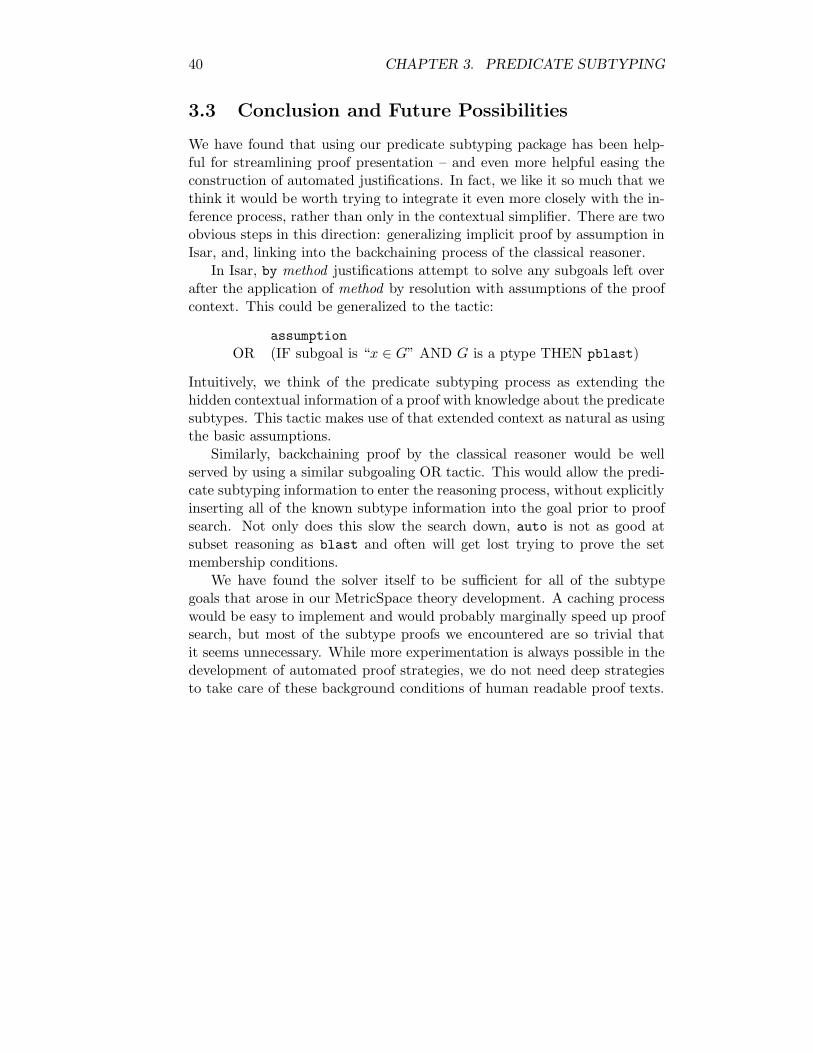
40 CHAPTER 3. PREDICATE SUBTYPING
3.3 Conclusion and Future Possibilities
We have found that using our predicate subtyping package has been help-ful for streamlining proof presentation – and even more helpful easing theconstruction of automated justifications. In fact, we like it so much that wethink it would be worth trying to integrate it even more closely with the in-ference process, rather than only in the contextual simplifier. There are twoobvious steps in this direction: generalizing implicit proof by assumption inIsar, and, linking into the backchaining process of the classical reasoner.
In Isar, by method justifications attempt to solve any subgoals left overafter the application of method by resolution with assumptions of the proofcontext. This could be generalized to the tactic:
assumption
OR (IF subgoal is “x ∈ G” AND G is a ptype THEN pblast)
Intuitively, we think of the predicate subtyping process as extending thehidden contextual information of a proof with knowledge about the predicatesubtypes. This tactic makes use of that extended context as natural as usingthe basic assumptions.
Similarly, backchaining proof by the classical reasoner would be wellserved by using a similar subgoaling OR tactic. This would allow the predi-cate subtyping information to enter the reasoning process, without explicitlyinserting all of the known subtype information into the goal prior to proofsearch. Not only does this slow the search down, auto is not as good atsubset reasoning as blast and often will get lost trying to prove the setmembership conditions.
We have found the solver itself to be sufficient for all of the subtypegoals that arose in our MetricSpace theory development. A caching processwould be easy to implement and would probably marginally speed up proofsearch, but most of the subtype proofs we encountered are so trivial thatit seems unnecessary. While more experimentation is always possible in thedevelopment of automated proof strategies, we do not need deep strategiesto take care of these background conditions of human readable proof texts.

Chapter 4
The Proof: Top View
The primary challenge in proving Stokes’ theorem is not the proof but thestatement itself. That is, the definitions and background theory involvedin merely stating the goal are far more complex than the proof, once thosedefinitions have been made. We have therefore attempted to distinguishbetween proof level and theory level design issues. Proof level issues haveto do with the structuring and writing of particular theorem proofs. Forinstance, given the theoretical framework (definitions, etc), how do we for-malize the proof of the uniqueness of vector space dimensionality? Whichsubgoals deserve lemma status, which should be solved automatically? Atthe theory level, we consider the structure of and interrelationships betweenthe high level concepts of the development. For instance, how we definevector spaces, which consist of constants, axioms and syntax, and how thosevector spaces build on abelian groups or relate to metric spaces are all theorylevel concerns.
In this and the next few chapters, we will attempt to describe the actualtheories written for this case study. The text of the proofs leading to theformal definition and properties of Euclidean n-space is included in the ap-pendix, with some suppression of details. Although we claim that the proofswe have written are readable and, as much as possible, enlightening, we donot claim that they are captivating. The roughly 75 pages of formal proofhave been developed independently of any textbook, but we estimate thatthe development as a whole is roughly 3-5 times as long as it would appearin an undergraduate text. There are some 450 lemmas and theorems andcountless named proof blocks local to large proofs.
This chapter takes a bird’s eye view of the proofs and describes theirmodular structure with reference to the ideas laid out in chapter 2.
41

42 CHAPTER 4. THE PROOF: TOP VIEW
4.1 Theory Structure
The top level strategy of this development has been to define and abstractlydevelop the various relevant mathematical structures (vector spaces, normedvector spaces, metric spaces, etc) and then attempt to bring them together todevelop more complicated theory (differentiability, etc), rather than simplyconstruct a specific theory of differential geometry from the ground up, oras an axiomatized whole. This strategy contrasts with the end goal orientedtheory development of many proof projects, but as a design choice, it followsimmediately from our desire for modularity.
Furthermore, we have attempted to build on as many published, existingtheories as possible, without modifying their text. Topological notions suchas continuity and open sets are provided by Friedrich’s Topology [9], theproperties of the real numbers are provided by Fleuriot’s Complex session[8] and the abelian group properties of real vector spaces are provided byBallarin’s Algebra session [2]. All of these are built on Isabelle’s HOL objectlogic.
In the next three sections, we will attempt to give a sense of the modularstructure of the development, with respect to Isabelle’s various packages forprogrammatic modularity described in chapter 2. That is, we will describethe top level organization of the theory files, record types representing cat-egories, and locales. As noted in §2.2, we have chosen not to use axiomatictype classes because they lack logical expressivity, and therefore they playno role in the organization of the proofs.
4.1.1 theory Organization
See figure 4.1 for the theory file dependence graph of the development.These files group related definitions and theorems in the same sense thatchapters of a book or books in a library group them. However, recall from§ 2.2 that theory objects do not simply provide the grouping for theo-rem, type and constant namespaces: they also provide (irrevocable) syntaxtranslation rules and the first layer of context containing the classical rule-set, simpset and predicate subtyping data. A theory that wishes to refer tosome other theory’s definitions or theorems must inherit it in toto, whichcan have various unexpected and difficult to debug consequences on auto-mated tool behavior and namespaces.
An Unexpected Conflict
Although Isabelle can correctly differentiate between constants with thesame name inherited from different theory files (but see § 7.1.1), it has nomeans to handle conflicts between syntax annotations. A particularly nastyconsequence of this means that there is no way to define an n-dimensional

4.1. THEORY STRUCTURE 43
MiscPrelimFiniteSum CardInj
VectorSpace
Subspace
LinearComb
FiniteVectorSpace
TopologyPredSubtype
MetricSpace
MetricTopology
MetricVectorSpace
[Pure]
[HOL]
[Algebra+Complex]
Figure 4.1: Graph of Isabelle Theory Level Dependencies. Solid lines in-dicate theory inheritance in the project; the dashed line indicates the con-flicting desired inheritance (see text). The bracketed boxes represent heapscompiled from the base Isabelle libraries. The Topology box is Friedrich’spoint-set topology theory. All other boxes correspond to files written forthis project.

44 CHAPTER 4. THE PROOF: TOP VIEW
derivative on Euclidean space in our development, because we cannot simul-taneously refer to a topology (which provides the notion of a limit) and avector space (which we need to define the function we want to take a limitof).
In particular, at the top of Ballarin’s Group theory, the constant carrieris defined as a field accessor:
record ′a partial-object =carrier :: ′a set
All of the algebraic structures in his theory are represented by extensionsof this record type. For example, since our vector space representation is anextension of his abelian groups, carrier V represents the carrier set of thevector space V .
In Friedrich’s Topology, a topology T is a set of open sets and the carrierset is defined as follows:
types′a top = ′a set set
constdefscarr :: ′a top ⇒ ′a set (carrier ı)carr T ≡ ⋃
T
Thus, carr T is the carrier set of topology T . However, Friedrich givescarr a structural syntax annotation of carrier (see § 2.2). From this an-notation onward, through children theory files, the system will attempt totranslate carrier into carr T , with T inferred. This clobbers any attemptto refer to the carrier V from the vector space theory.
We have marked a desired inheritance on the theory graph 4.1 from Met-ricTopology to MetricVectorSpace. This inheritance does not exist becauseof this conflict. The best we can do is show that a normed vector space hasa natural metric space structure, as is done in MetricVectorSpace, withoutbeing able to use the induced topological structure defined in MetricTopol-ogy.
Of course, it would be trivial to modify Friedrich’s Topology to removethe syntax annotation (or rename it) so that this conflict would disappear.We have not done this because from a group engineering point of view, wefeel it is important to be able to use existing theories without modifyingthem. Glibly, we should not need to rewrite Bourbaki in order to refer totheir results. This conflict illustrates the need for some careful rethinking ofthe relationship between Isabelle’s parsing and its modular structures (see§ 7.1 for some of our thoughts on the matter).

4.1. THEORY STRUCTURE 45
Record Type Field Accessors Accessor Type
α partial object carrier αset
α semigroup mult α⇒ α⇒ α
α monoid one α
α ring zero αadd α⇒ α⇒ α
α realvectorspace t rprod real ⇒ α⇒ α
α finitevectorspace t std basis αset
Table 4.1: The Linear Inheritance Structure of Algebraic Record Types.Each row inherits from the previous row. We have left out the preliminaryαrecord type⇒ in the last column.
4.1.2 Record Organization
Table 4.1 shows all of the record types used in the representation of algebraiccategories, from Ballarin’s Group theory through our FiniteVectorSpace the-ory. We have inherited the locale + record representation of his abeliangroups and extended it directly into a theory about real vector spaces:record ′a realvectorspace-t = ′a ring +rprod :: [real , ′a] ⇒ ′a (infixr ·ı 70 )
locale realvectorspace = abelian-group V +assumes rprod-closed [simp,intro]: x ∈ carrier V =⇒ a · x ∈ carrier V
and add-rprod-distrib1 : [[x ∈ carrier V ; y ∈ carrier V ]] =⇒ a · (x ⊕ y) = a· x ⊕ a · y
and add-rprod-distrib2 : x ∈ carrier V =⇒ (a + b) · x = a · x ⊕ b · xand rprod-assoc: x ∈ carrier V =⇒ (a ∗ b) · x = a · (b · x )and rprod-1 [simp]: x ∈ carrier V =⇒ 1 · x = xand negate-eq1 : x ∈ carrier V =⇒ x = (− 1 ) · x
Because of the locale inheritance and polymorphism of the ring andrealvectorspace t types, all of the lemmas, simpset and ruleset related toabelian groups are immediately available for our real vector spaces. Strangely,this requires us to extend the ring record type and ignore its mult and one
fields, because this is how Ballarin has represented additive notation basedabelian groups.
We have not used records to represent the category of metric spacesbecause we wished to explore the impact of using fully expanded localeparameterizations (see § 4.1.3) and we did not have any precursor theoriesto extend.

46 CHAPTER 4. THE PROOF: TOP VIEW
T::’a toptopobase B::’a set set
T::’a topcarrier
metricbase M::’a set D::’a metric B::’a set set
premetricspace M::’a set D::’a metric
topology T::’a topM::’a set D::’a metricmetricspace
realvectorspace V::’a realvectorspace_t
abelian_monoid G::’a ring
abelian_group G::’a ring
subspace U V::’a realvectorspace_t
comm_monoid G::’a monoid
comm_group G::’a monoid
finitevectorspace V::’a finitevectorspace_t
rvs_dim_proof
In Friedrich’s Topology
metrictop M::’a set D::’a metric B::’a set set T::’a top
euclideanspace V::’a finitevectorspace_t M::’a set D::’a metric B::’a set set T::’a top
Desired Next Step
In Ballarin’s Algebra
Figure 4.2: Graph of Locale Dependencies. Black arrows indicate localeinheritance; white arrows indicate logical connection (theorems could liftalong the direction of the arrow). The dashed box indicates the locale thatwe would next define if there were no conflict between Topology and Algebra.
4.1.3 Locale Organization
Figure 4.2 depicts the interrelationships of the locales used in the develop-ment. The Complex session does not appear in the locale graph becausethe properties of the reals are organized by the type real, rather than in alocale context. The potential relationships between locales are substantiallymore complicated than the simple multiple-inheritance structure availableto theory files: not only do locales have complicated inheritance/merge se-mantics (see § 2.2 and [3]), they are also associated with predicates withinthe logic and therefore can use one another without being related in theinheritance structure. Thus, we have added a second kind of arrow to thegraph to indicate where theorems from a particular locale could be liftedthrough the logic into another.
To illustrate the meaning and impact of the white-tipped arrows, weconsider the connection between comm group and abelian group. In the Al-gebra session, Ballarin develops the category of commutative groups basedon the record type for monoids with product-style syntax. The commutativering theory then defines the category of abelian groups by using the addi-tive structure of a ring record and assuming that the fields (V, .., ..,+, 0)constitute a commutative group when repackaged as (V,+, 0). This is whatone has to do to change formal parameterization of a locale-based theory;unfortunately, it requires roughly 250 lines of manual lemma lifting to makethe basic properties of commutative groups available for abelian groups.
The box labeled “Desired Next Step” corresponds to the desired link inthe theory graph (figure 4.1). From a logical point of view, we have defined

4.2. REUSING EXISTING MATERIAL: TYPES, LOCALES, PARAPHRASING47
and proved all of the connections necessary to connect normed vector spacesto their topology. In the MetricVectorSpace theory, we prove:
constdefsstd-dist :: ( ′a, ′m) basisvectorspace-t-scheme ⇒ ′a ⇒ ′a ⇒ real (dist ı 1000 )std-dist V a b ≡ std-norm V (minus V a b)
theorem (in finitevectorspace) metricspace (carrier V ) dist
And in the MetricTopology theory, we prove:
lemma metrictopI : metricspace M D =⇒ metrictop M D
By resolution we should have that metrictop(carrierV )dist, and weshould be able to naturally define the Euclidean space given by a finitedimensional real vector space with the usual metric, δ(x, y) = ‖x − y‖. Asdescribed in §4.1.1, this is prevented by a syntactic conflict.
4.2 Reusing Existing Material: Types, Locales,
Paraphrasing
There are three essential kinds of reuse of pre-existing material in this de-velopment:
• type use, in which we make use of well developed types like real andnat;
• locale inheritance, in which we inherit from and extend Ballarin’sabelian groups into real vector spaces;
• paraphrasing, in which we closely followed the initial developmentof the HahnBanach theory vector spaces when redeveloping them interms of a locale + record structure
Of the kinds of reuse listed above, the most transparent to the developerand the human reader is the first. As mentioned in § 2.2, theory which fitsinto simple types just works well – constants, syntax, axioms and theoremsare all immediately available to appropriately typed expressions, and thetyping process is largely behind the scenes. There is no need to explicitlyconstruct a locale context for a given theorem (they are all global) and thereare some special automated proof procedures for the arithmetic types thatkick in largely transparently as well.
Using somebody else’s locales is quite a bit more tricky than using theirtypes. In our development, the mathematical concept of a vector spaceis given by a locale which inherits from Ballarin’s abelian group locale,
48 CHAPTER 4. THE PROOF: TOP VIEW
assumes the additional vector space axioms and fixes a formal parameterof record type realvectorspace t. realvectorspace t extends Ballarin’sring type and looks like (V, 1, ∗, 0,+, ·), where the second and third fieldare ignored. Here we see some unavoidable machine-directed noise: eitherwe use this unseemly type construction or we could not inherit the abeliangroup locale and all of its theorems in one fell swoop. Unfortunately, thegeneral principle of using a single record parameter to hold all of the formalparameters of an axiomatized structure (imposed on us by the decision toextend the Algebra session) means that we lose much of the flexibility of thelocale merge and inheritance semantics, because record inheritance is muchmore restrictive.
Of course, whether one is reusing a type-based theory or a locale-basedone, it is quite likely that some additional lemmas will need to be proved thatconceptually belong in the previous development. This is a problem in anykind of modular, multideveloper project, but is exacerbated in formal proofby the fact that it is impossible to fix the limits of what should constitute amodule’s functionality. In OOP terminology, what interface should the classfor Real numbers provide? In attempting to extend Ballarin’s abelian groupalgebra, we found it necessary to substantially extend the basic lemmasabout the finite sum operation over abelian groups (see appendix). We havealso had to prove lemmas about real numbers (like the quadratic formula,see chapter 5) and a few notes on pure point-set topology.
It is not visible in any of the modular graphs we have presented above,but it is important to mention that the first several pages of developmentrelated to vector spaces (their definitions, etc) are essentially a paraphraseof the vector space development from the Hahn-Banach proof given in [4]).This development was done using axiomatic type classes and it was an in-teresting exercise to see just how easily most of the proofs translated. Mostof the basic lemmas required only two adjustments: the addition of thetext “(in realvectorspace)” to declarations of lemmas; and, the addition ofconditions of the form x ∈ carrier V to their statements. As the lemmasbecame more complicated, the proofs themselves began to change becauseautomated tools started failing or behaving differently. That we had torewrite this basic definitional theory of vector spaces is an implicit criticismof the system: ideally, a definition of vector space is a definition of vectorspace is immediately reusable in a theory that wants to use or extend vectorspaces.
This last criticism is perhaps unfair: we wanted to build on the devel-opment of the Algebra session and at the same time use the developmentin the HahnBanach proof. Why should they be immediately compatible?No systems programmer would expect such a miracle when attempting tomerge two independently written libraries. However, this is exactly whata mathematician would expect: there are umpteen different popular textson linear algebra, and hundreds of different teachers at universities, but all

4.3. CONCLUSION 49
of the students from those different traditions can talk to each other aboutkernels and linear transformations.
4.3 Conclusion
In this chapter, we have described the case study at a theory level. We haveattempted to set its modular structures into the context provided by chapter2 and noted some key development difficulties that are visible even from thisbird’s eye view. We leave the exploration of particular issues in readabilityand translating mathematical vernacular to the next two chapters, that havebeen generated from the Isabelle sources directly. They are organized bytheir mathematical content, rather than any theoretical model of modularityor readability.

Chapter 5
The Proof: Vector SpaceHighlights
This chapter has been generated entirely from the Isabelle source of ourcase study. In it, we have highlighted several proofs from the developmentof real vector spaces, without giving the full definitional build-up. Unlike themetric space-related theories, which we present in their entirety in the nextchapter, the development of linear algebra is long and occasionally tedious.This is because it develops a complete basic framework of linear algebra fromthe vector space axioms up and contains a large number of support lemmasrelated to calculation and the basic properties of linear combinations. It isincluded in a more complete form in the Appendix.
The first proof we present as a bit of a warm-up to Isabelle/Isar stylecalculational proofs. The quadratic formula is integral to the proof of theSchartz inequality of the standard norm, in the FiniteVectorSpace theory.Its proof is relatively short but illustrates some of the difficulty of writingexpressive but verifiable proofs.
In the next section, we present one of the deepest results of the entiredevelopment: that the dimension of finite vector spaces is well-defined. Thisproof was extremely difficult to formalize and is much more technical thanmost of the rest of the theory we have developed. It is something of aworst case in our attempts to turn mathematically communicative proofsinto formally verified proofs.
5.1 Highlight: Quadratic Formula
The roots of a quadratic polynomial ax2 + bx + c with a 6= 0 are given bythe formula
−b±√b2 − 4ac
2a
50

5.1. HIGHLIGHT: QUADRATIC FORMULA 51
In particular, the quantity b2 − 4ac is called the discriminant of the polyno-mial ax2 + bx+ c and its sign determines the number of real roots, 0, 1 or2.
In order to prove the Schwartz inequality later, we will need a part ofthe above quadratic theorem: that a non-negative discriminant implies theexistance of a solution. Euphemistically, this implication can be shown bya “plug-and-chug” proof: we assume that the discriminant is nonnegative,plug the quadratic formula into our quadratic polynomial and evaluate theexpression to show it is 0.
In Isabelle, the primary tool for expression evaluation is the simplifier.Unfortunately, blind rewriting is not a terribly effective strategy for simpli-fying non-linear algebraic expressions. The following “simple” proof tookapproximately two hours to develop, as we struggled with guiding the sim-plifier through the evaluation while also trying to maintain a readable text.
To simplify the expressions we had to work with, we eventually wrote alemma for the monic case, where a = 1, and then proved the general caseby reducing it to the monic.
theorem quadratic-formula-monic:assumes disc: 0 ≤ b2 − 4 ∗ c (is 0 ≤ ?disc)shows ∃ (x ::real). x 2 + b∗x + c = 0
prooflet ?x = − b / 2 + (sqrt ?disc) / 2
— First, evaluate ?x2
have ?x 2 = b2/4 − 2∗b∗(sqrt ?disc) / 4 + (sqrt ?disc)2 / 4by (simp add : power2-eq-square ring-eq-simps)
also have . . . = b2/4 − 2∗b∗(sqrt ?disc) / 4 + ?disc / 4using disc by (simp only : real-sqrt-ge-zero-pow2 )
also have . . . = b2/2 − (b∗sqrt ?disc) / 2 − cby (simp only : divide-inverse) (simp add : ring-eq-simps)
finally have first-term: ?x 2 = b2/2 − (b∗sqrt ?disc)/2 − c .
— Now plug it in and let the ring simprocs take over.show ?x 2 + b ∗ ?x + c = 0apply (simp only : first-term)by (simp only : divide-inverse) (simp add : ring-eq-simps power2-eq-square)
qed
The general theorem should be a simple reduction, where we divide ev-erything through by a. Massaging this division process into just the rightform to use the monic lemma is quite difficult. Any secondary school math-ematician should be able to follow the calculations, but the steps are notwhat most people would write to “show their work” to the teacher.
theorem quadratic-formula:assumes disc: 0 ≤ b2 − 4 ∗ a ∗ c (is 0 ≤ ?disc)
and anz : a 6= 0

52 CHAPTER 5. THE PROOF: VECTOR SPACE HIGHLIGHTS
shows ∃ x . (a::real) ∗ x 2 + b ∗ x + c = 0proof −have 0 ≤ (b / a)2 − 4 ∗ (c / a)proof −from anz have 0 ≤ inverse (a2) by simpwith disc have 0 ∗ inverse (a2) ≤ (b2 − 4 ∗ a ∗ c) ∗ inverse (a2)by (rule mult-right-mono)
hence 0 ≤ (b2 − 4 ∗ a ∗ c) ∗ inverse (a2) by simpalso from anz have . . . = (b / a)2 − 4 ∗ (c / a)by (simp only : divide-inverse power2-eq-square) (simp add : ring-eq-simps)
finally show 0 ≤ (b / a)2 − 4 ∗ (c / a) .qed
with quadratic-formula-monicobtain x where monic: x 2 + (b / a) ∗ x + (c / a) = 0by blast
show ∃ x . a ∗ x 2 + b ∗ x + c = 0proof
— This subproof should be automatic, but it takes work with a simplifier.have 0 = a ∗ 0 by simpalso from monic have . . . = a ∗ (x 2 + (b / a) ∗ x + (c / a)) by simpalso have . . . = a ∗ x 2 + (a / a) ∗ b ∗ x + (a / a) ∗ cby (simp add : ring-eq-simps)
also from anz have . . . = a ∗ x 2 + b ∗ x + c by simpfinally show a ∗ x 2 + b ∗ x + c = 0 ..
qedqed
5.2 Highlight: Uniqueness of Dimensionality
We wish to prove the following result about abstract vector spaces:
Theorem 5.2.1 If a vector space V has a finite basis, then all other basesare also finite and have the same cardinality.
Thus, we will be able to uniquely define the dimension of a vector spaceas the cardinality of a representative basis.
The proof relies on an essentially algorithmic argument. Informally,suppose that we have two bases, A = a, b, c, d and B = x, y, z. Since Bspans, we can add a to B to form a linearly dependent set a, x, y, z. Sincethis set is linearly dependent and a is linearly independent, we can solvefor one of the members of a, x, y, z not in a. Say we solve for z. Thus, z ∈span a,x ,y and we can remove z from a, x, y, z to get a new spanning setB′ = a, x, y. Now we repeat, choosing a new element from A and removinganother element of B from B ′ for each iteration.

5.2. HIGHLIGHT: UNIQUENESS OF DIMENSIONALITY 53
Eventually, we will end up with a spanning set a,b,c ⊂ A. But this isa contradiction because A is linearly independent and cannot be containedin the span of a proper subset. Thus, A and B must have the same numberof elements.
The formalization of the above essentially simple argument is massive –roughly 10 pages of technical arguments. We spent about a week trying tofigure out how best to represent the inductive process and prove its invari-ants. Eventually, we decided to use Isabelle’s recdef package1 to define atail-recursive function of 3 arguments that “does” the transfer process andreturns the final set B ′′ ⊂ A from which we get a contradiction.
Before diving into the formalization, we note that we have very mixedfeelings about this proof: on the one hand, it is a fundamental theoremthat allows us to define the fundamental concept of dimension for abstractvector spaces. After a week of frustration, the final qed was accompanied byjubilation. On the other hand, although we tried to capture the structural“soul” of the informal proof by encoding it directly into a recursive process,the resulting argument is so technical and complicated that it has lost all ofits elegance and readability. The intuitive content is gone.
Of course, the informal proof is a “proof by example”, and one thatglosses over the complexities of allowing a potentially infinite set for A. Itis perhaps a mathematical bad habit to consider it a good proof, but itcertainly distills out the intuitive content of the theorem.
Intuitive Formalization
In order to motivate the definitions that follow, we will restate the informalproof given above in somewhat more suggestive terms:
Start with two bases, A and B, and assume A has more elements thanB. Then, apply the following algorithm:
1. Choose an a ∈ A that has not been previously chosen.
2. Transfer the chosen a to the set B.
3. Choose a b ∈ B, not originally from the set A, that we can solve forin terms of the other elements of B.
4. Discard our chosen b from B.
5. Repeat until all the original elements of B have been discarded.
The resulting B provides a contradiction because it is a spanning set, anda proper subset of A and A is supposed to be linearly independent.
1recdef allows the definition of arbitrary recursive functions by proving that they are
well-founded and terminating.
54 CHAPTER 5. THE PROOF: VECTOR SPACE HIGHLIGHTS
Some observations: the algorithm only terminates if B is initially finite.This will be a condition of the final theorem as well. Also, there are twochoices in the process. They will eventually turn into a pair of dependentHilbert choices at each step of the recursive function call. The choice stepsdepend on the set of elements that have been transferred so far in the process.This suggests that we can simplify the conditions on the choice steps if wekeep track of the set T of transferred elements. With these observations, wepresent the final version of the algorithm:
We start with two bases, A and B, and an empty set T , that will holdthe elements that have been transferred from A to B. Now, we state thealgorithm recursively:
If B = stop, otherwise do the following:
1. Choose any a ∈ A.
2. Note that B ∪ T spans and therefore B ∪ T ∪ a is linearly dependent.
3. Note that T ∪ a is linearly independent because it is a subset of thebasis A.
4. Therefore, choose an element b ∈ B that we can solve for in terms ofthe other elements of B ∪ T ∪ a.
5. Recur, letting A = A− a, T = T ∪ a and B = B − b.
When the algorithm stops, T ⊂ A provides the contradiction we want.This is the essence of the algorithmic proof which we have formalized
below. We will present the definitions and statements of lemmas, but sup-press most of the proofs, which are technically very complicated but notespecially interesting. They are also unavoidably hard to read because ofthe number of conditions they involve.
Formal Text
The following mass of definitions and lemmas should all be local to theeventual theorem about dimensionality uniqueness, which is all we will wantto use later. Thus, we create an empty locale and prove all of the lemmasin that locale – if a lemma depends on the realvectorspace structure, it isincluded rather than targeted. We export only the final theorem into therealvectorspace locale.
locale rvs-dim-proof
The following function returns the pair of choices made at each step ofthe recursive procedure. The ε is Hilbert’s indefinite descriptor. We couldread the function definition as returning “Some pair (a, b) such that a ∈ A,b ∈ B and B ∪ T ∪ a spans the vector space V.”

5.2. HIGHLIGHT: UNIQUENESS OF DIMENSIONALITY 55
constdefsbasis-elim :: ( ′a, ′b) realvectorspace-t-scheme ⇒ ′a set ⇒ ′a set ⇒ ′a set ⇒
′a × ′abasis-elim V A B T ≡ ε (a,b). a ∈ A ∧ b ∈ B
∧ span-set V ((B ∪ T ∪ a) − b) = carrier V
There are quite a few necessary conditions for the above choice functionto be well-defined. The following predicate encapsulates them. The notationB → A means that there is an injection from the set B to the set A (intu-itively, A is at least as “big” as B). We have developed a fairly substantialtheory of this injection relation in CardInj.thy, see the appendix.
constdefsbasis-elim-is-def :: ( ′a, ′b) realvectorspace-t-scheme ⇒ ′a set ⇒ ′a set ⇒ ′a set
⇒ boolbasis-elim-is-def V A B T ≡ realvectorspace V
∧ B 6= ∧ (A ∩ B = ) ∧ (A ∩ T = ) ∧ (B ∩ T = )∧ B ⊆ carrier V∧ B → A
∧ span-set V (B ∪ T ) = carrier V ∧ is-basis-on V (A ∪ T )
The following lemma proves that the conditions represented by basis elim is def
actually lead to the existence of the basis elim choice. We have not excisedthe proof from the presentation because we feel it is actually fairly readable,just complicated by all of the technical conditions. One of the problems isthat we refer to assumptions and partial results by abbreviated names thatcan be hard to digest. This relates to the classic programming trade-offbetween descriptive variable names and ease of typing.
lemma (in rvs-dim-proof ) basis-elim-ex :includes realvectorspace Vassumes disjAB : A ∩ B = and disjAT : A ∩ T =
and Bnonempty : B 6= and Bsubcar : B ⊆ carrier V and spansBT : span (B ∪ T ) = carrier Vand BleA: B → A and isBasisAT : isBasis (A ∪ T )
shows ∃ (a,b) ∈ UNIV . a ∈ A ∧ b ∈ B ∧ span-set V (B ∪ T ∪ a − b) =carrier Vproof −from BleA Bnonempty have A 6= ..then obtain a where ainA: a ∈ A by blast
with disjAB disjAT have anotB : a /∈ B and anotT : a /∈ T by auto
from isBasisAT have ATsubcar : A ∪ T ⊆ carrier V by autohence Asubcar : A ⊆ carrier V and Tsubcar : T ⊆ carrier V by auto
have li-Ta: linearind (T ∪ a)proof (rule sub-linearindI )from isBasisAT show linearind A ∪ T ..
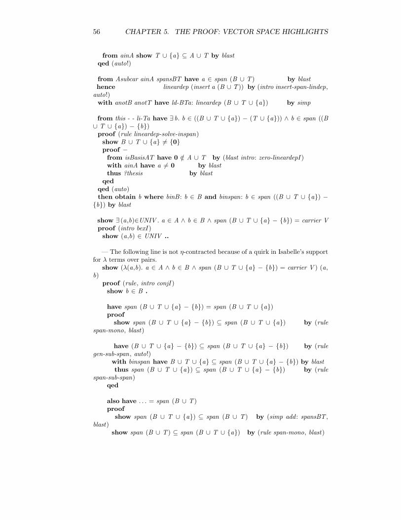
56 CHAPTER 5. THE PROOF: VECTOR SPACE HIGHLIGHTS
from ainA show T ∪ a ⊆ A ∪ T by blastqed (auto!)
from Asubcar ainA spansBT have a ∈ span (B ∪ T ) by blasthence lineardep (insert a (B ∪ T )) by (intro insert-span-lindep,
auto!)with anotB anotT have ld-BTa: lineardep (B ∪ T ∪ a) by simp
from this - - li-Ta have ∃ b. b ∈ ((B ∪ T ∪ a) − (T ∪ a)) ∧ b ∈ span ((B∪ T ∪ a) − b)proof (rule lineardep-solve-inspan)show B ∪ T ∪ a 6= 0proof −from isBasisAT have 0 /∈ A ∪ T by (blast intro: zero-lineardepI )with ainA have a 6= 0 by blastthus ?thesis by blast
qedqed (auto)then obtain b where binB : b ∈ B and binspan: b ∈ span ((B ∪ T ∪ a) −
b) by blast
show ∃ (a,b)∈UNIV . a ∈ A ∧ b ∈ B ∧ span (B ∪ T ∪ a − b) = carrier Vproof (intro bexI )show (a,b) ∈ UNIV ..
— The following line is not η-contracted because of a quirk in Isabelle’s supportfor λ terms over pairs.
show (λ(a,b). a ∈ A ∧ b ∈ B ∧ span (B ∪ T ∪ a − b) = carrier V ) (a,b)
proof (rule, intro conjI )show b ∈ B .
have span (B ∪ T ∪ a − b) = span (B ∪ T ∪ a)proof
show span (B ∪ T ∪ a − b) ⊆ span (B ∪ T ∪ a) by (rulespan-mono, blast)
have (B ∪ T ∪ a − b) ⊆ span (B ∪ T ∪ a − b) by (rulegen-sub-span, auto!)
with binspan have B ∪ T ∪ a ⊆ span (B ∪ T ∪ a − b) by blastthus span (B ∪ T ∪ a) ⊆ span (B ∪ T ∪ a − b) by (rule
span-sub-span)qed
also have . . . = span (B ∪ T )proof
show span (B ∪ T ∪ a) ⊆ span (B ∪ T ) by (simp add : spansBT ,blast)
show span (B ∪ T ) ⊆ span (B ∪ T ∪ a) by (rule span-mono, blast)

5.2. HIGHLIGHT: UNIQUENESS OF DIMENSIONALITY 57
qed
finally show span (B ∪ T ∪ a − b) = carrier V by (simp add : spansBT )qed
qed
qed
The next lemma simply abbreviates the previous one using the basis elim is def
predicate.
lemma (in rvs-dim-proof ) basis-elim-is-defD [dest ]: basis-elim-is-def V A B T=⇒ ∃ (a,b) ∈ UNIV . a ∈ A ∧ b ∈ B ∧ span-set V (B ∪ T ∪ a − b) =
carrier V
by (intro basis-elim-ex , auto simp add : basis-elim-is-def-def )
And the following lemma states that, given the definedness condition,the pair returned by the basis elim function has the properties we want.We suppress the proof because it follows trivially from the existence provedabove and the definition of the Hilbert ε.
lemma (in rvs-dim-proof ) basis-elim-props [dest , simp]:assumes be: basis-elim-is-def V A B T
and ab: (a, b) = basis-elim V A B T
shows a ∈ A b ∈ B span-set V (B ∪ T ∪ a − b) = carrier V
Now that we have all the properties we wanted about the choices in-volved in our recursive algorithm, we are almost ready to define the actualbasis-transfer function. However, before we do so, we need one more tech-nical lemma that will be used by the recdef package to show that ouralgorithm is terminating, so long as it is called with the appropriate con-ditions. The following lemma essentially says that, so long as B is finiteand the choice conditions hold, |B| decreases with each recurrence and theprocedure will terminate.
lemma basis-transfer-term: ∀ A B T V a b. (a, b) = basis-elim V A B T∧ finite B ∧ basis-elim-is-def V A B T −→(B − b, B) ∈ finite-psubset
Finally, we can define the basis transfer function. It does exactlywhat we described above in the final version of our algorithm, but it hasextra conditions to make it return immediately (without recurring) if the Bis infinite or the conditions for making the choices fail to hold. This makesit well-defined for the entire universe of possible inputs, which is requiredby the total logic used in Isabelle/HOL.
constsbasis-transfer :: ′a set × ′a set × ′a set × ( ′a, ′b) realvectorspace-t-scheme ⇒ ′a
set
recdef (permissive) basis-transfer inv-image finite-psubset (λ(a,b,t ,v). b)basis-transfer(A, B , T , V ) = (if (finite B ∧ basis-elim-is-def V A B T )

58 CHAPTER 5. THE PROOF: VECTOR SPACE HIGHLIGHTS
thenlet (a,b) = (basis-elim V A B T ) in (
basis-transfer(A − a, B − b, T ∪ a, V ))
elseT
)
( hints recdef-wf add : wf-finite-psubset )
We prove the three properties of the result of the basis transfer func-tion that together constitute the contradiction we need to finish the proof.All three are proved by induction on the recursion rule provided by therecdef package.
lemma (in rvs-dim-proof ) basis-transfer-sub-AT : basis-transfer(A, B , T , V ) ⊆ A∪ T
lemma (in rvs-dim-proof ) basis-transfer-card : finite B −→ finite T −→finite (basis-transfer(A, B , T , V )) ∧ card (basis-transfer(A, B , T , V ))
≤ card (B ∪ T )
lemma (in rvs-dim-proof ) basis-transfer-spans : realvectorspace V −→ finite B −→
A ∩ B = −→ A ∩ T = −→ B ∩ T = −→B ⊆ carrier V −→ B → A −→span-set V (B ∪ T ) = carrier V −→ is-basis-on V (A∪T ) −→
(span-set V (basis-transfer(A, B , T , V )) = carrier V )
Nearly there! The following lemma shows that if B is a finite basis, andB → A, with A another basis, then A is actually finite and has the samenumber of elements as B. This is the heart of the proof, in which we “call”the basis transfer function and show that it leads to a contradictory resultunless |A| = |B|.
The proof itself is readable to a developer, but like the lemmas above it,has so many separate facts and conditions that the gist of the mathematicsis obscured. We have accordingly suppressed it.
lemma (in rvs-dim-proof ) unique-dimension-a:includes realvectorspaceassumes finB : finite B
and basisA: isBasis Aand basisB : isBasis Band BinjA: B → A
shows finite A ∧ card A = card B
The final theorem follows the previous lemma by a case split on thepossible size relationships between A and B.
theorem (in realvectorspace) unique-dimensionI :assumes finB : finite B

5.2. HIGHLIGHT: UNIQUENESS OF DIMENSIONALITY 59
and basisA: isBasis Aand basisB : isBasis B
shows finite A ∧ card A = card Bproof (rule classical)instantiate rvs-dim-proofassume neg : ¬ (finite A ∧ card A = card B)
henceAbig-or-Bbig : (infinite A ∨ (finite A ∧ card B < card A))
∨ (finite A ∧ card A < card B) by auto
show ?thesisproof (cases rule: Abig-or-Bbig [THEN disjE , case-names Abigger Bbigger ])case Abigger
hence BinjA: B → Aby (rule disjE , insert finB , auto intro: cardinj-fin-infI cardinj-fin-cardI )
from - finB basisA basisB BinjA show ?thesis by (rule unique-dimension-a,auto)
nextcase Bbigger
hence AinjB : A → Bby (insert finB , auto intro: cardinj-fin-cardI )
from this finB have finA: finite A ..
from - finA basisB basisA AinjBhave finite B ∧ card B = card A by (rule unique-dimension-a, auto)
with finA show ?thesis by simpqed
qed

Chapter 6
The Proof: Metric Spaces
theory MetricSpace = PredSubtype + MiscPrelim:
This chapter has been generated entirely from the Isabelle source of ourcase study. It is a nearly complete presentation of the development of metricspaces, metric topologies and finally, metrics on normed vector spaces. Wehave written extended mathematical and technical commentary to attemptto place the development in its context and link it to the more abstractdiscussions found in the previous chapters. Unlike the linear algebra theory,which we have merely excerpted, this development is shorter and sweeter,has a high concentration of interesting theorems and illustrates several of thefundamental problems encountered in trying to develop a modular theorystack.
Metric spaces are the category of sets with distances (metrics) on them.According to [6],
Definition A metric space is a set endowed with a metric; this induces atopology on the set in which Ω is open if and only if for all x ∈ Ω, there is apositive ε such that the open ball Bε(x) is contained in Ω.
Definition A metric is a non-negative symmetric binary function definedfor a given set, often denoted δ(x, y) and referred to as distance, that satisfiesthe triangle inequality
δ(x, y) + δ(y, z) ≤ δ(x, z)
and is zero only if x = y.
In our formalization, we will additionally require that M is non-empty,although this should perhaps be an orthogonal categoric structure.
Technically, our metric space theory has several interesting characteris-tics:
60

6.1. PRELIMINARIES 61
• We use our predicate subtyping package (see chapter 3) to managethe membership conditions of M . This transparently discharges manysubgoals and simplifies the construction of justifications.
• We do not use a record parameter to store M and δ. Instead, theyare two separate formal parameters to the locale metricspace. Thisminor representational decision has large consequences on the natureof the development.
Because of the latter choice, it is hard to define theory-level constantsfor metric spaces: they need two structural parameters instead of just arecord parameter. Therefore, we have also used the definitional facilitiesavailable in locales to define open balls as locale parameters. This allows usto define oB with respect to both M and D directly, without making themformal parameters to the symbol.
As a general procedure for defining constants, this does not scale:
• We cannot create new definitions in the metric space locale after thetime of creation. If we later decide we want a closed ball symbol, cB,we will have to go back and add it to our locale definition, which willextend the -arity of the locale parameter list, or create a new namedlocale.
• The formal parameters of a locale form a list of arguments to the locale.Defining symbols within the locale extends this list. Especially as wemerge locale contexts to reason about multiple underlying spaces, theparameter lists can become unmanageably long.
For presentation purposes, we have removed the proofs of a few trivialtechnical lemmas from the following presentation of metric spaces, metrictopologies and metric vector spaces. We have attempted to comment inlineon the development where either mathematical or technical points arise.
6.1 Preliminaries
6.1.1 Definition
types′a metric = [ ′a, ′a] ⇒ real
A technical note: we cannot use the locale defines construct to define aformal parameter D after D has been used in an assumption. Therefore, wecreate the premetricspace locale so that we can inherit from it, define D inan intermediate locale (for instance in terms of the norm of a vector space)and then inherit the metric space assumptions. This is slightly awkward butensures consistency of definitional constructs.

62 CHAPTER 6. THE PROOF: METRIC SPACES
locale premetricspace = var M + var D
locale metricspace = premetricspace +
— Here we define the open ball of radius r at x as a locale constant.fixes oB :: [real , ′a] ⇒ ′a setdefines oB r x ≡ y . y ∈ M ∧ D x y < r
— The metric space axioms + non emptinessassumes non-empty [simp, intro]: M 6= and positive [simp, intro]: [[x ∈ M ; y ∈ M ]] =⇒ 0 ≤ D x yand definite-eq [intro]: [[x ∈ M ; y ∈ M ]] =⇒ D x y = 0 =⇒ x = yand definite-zero [intro]: [[x ∈ M ; y ∈ M ]] =⇒ x = y =⇒ D x y = 0and symmetric: [[x ∈ M ; y ∈ M ]] =⇒ D x y = D y xand triangle: [[x ∈ M ; y ∈ M ; z ∈ M ]] =⇒ D x z ≤ D x y + D y z
— Declare M as a predicate subtype.lemma (in metricspace) [ptype]: ptype M ..
6.1.2 Basic Properties
We suppress the proofs.
lemma (in metricspace) dist-self-zero [simp, intro]:assumes [pfact ]: x ∈ M shows D x x = 0
lemma (in metricspace) dist-gt-zero [simp,intro]:assumes [pfact ]: x ∈ M y ∈ M and x 6= yshows 0 < D x y
lemma (in metricspace) dist-self-ltr [simp, intro]:assumes [pfact ]: x ∈ M and 0 < rshows D x x < r
6.1.3 Open Balls
We make the following lemma a predicate subtyping fact so that we neednot worry that y ∈ oBrx =⇒ y ∈M .
lemma (in metricspace) oball-subset [pfact ]:shows oB r x ⊆ M
lemmas (in metricspace) in-ball-in-space [dest ] = oball-subset [THEN subsetD ]
lemma (in metricspace) in-ball-iff :assumes [pfact ]: x ∈ M y ∈ Mshows (D x y < r) = (x ∈ oB r y)
lemma (in metricspace) in-ballI [intro]: [[D x y < r ; x ∈ M ; y ∈ M ]] =⇒ x ∈ oBr ylemma (in metricspace) in-ballD [dest ]: [[x ∈ oB r y ; x ∈ M ; y ∈ M ]] =⇒ D x y< rlemma (in metricspace) empty-ball-iff :assumes [pfact ]: x ∈ M

6.1. PRELIMINARIES 63
shows (r ≤ 0 ) = (oB r x = )lemma (in metricspace) has-value-has-radius :assumes [pfact ]: y ∈ M and xb[pfact ]: x ∈ oB r y
shows 0 < r
This lemma is considered in considerable detail as the example in chapter3
lemma (in metricspace) concentric-ball-subset :assumes radii : r1 ≤ r2 and [pfact ]: x ∈ Mshows oB r1 x ⊆ oB r2 x
6.1.4 Distance Implies Disjointness
The following lemma formalizes the idea that two balls whose centers arefurther apart than the sum of their radii are disjoint. It is required for theproof of the Hausdorff property of the metric topology.
It is a great example of a calculational reasoning-style proof, and wefeel that it stands on its own quite nicely. A normal textbook presentationwould be accompanied by a picture like that in figure 6.1.
yrxr
d(x,y)x y
Figure 6.1: The geometric intuition behind the lemma far imp disjoint balls.
A note on proof style here: the is pattern matching construction allowsus to abbreviate the two open balls by ?Bx and ?By.
lemma (in metricspace) far-imp-disjoint-balls :assumes rx + ry < D x y and [pfact ]: x ∈ M y ∈ Mshows oB rx x ∩ oB ry y = (is ?Bx ∩ ?By = )
proof (rule ccontr)assume ?Bx ∩ ?By 6= then obtain z where [pfact ]: z ∈ ?Bx z ∈ ?Byby blast
hence a: D x z < rx and b: D y z < ry by (auto simp add : oB-def )
have D z y = D y z by (simp only : symmetric)

64 CHAPTER 6. THE PROOF: METRIC SPACES
with b have D z y < ry by (simp)from a this have D x z + D z y < rx + ry by (simp)also have . . . < D x y .finally have D x z + D z y < D x y .hence ¬ (D x y ≤ D x z + D z y) by (simp add : linorder-not-le)
moreover have D x y ≤ D x z + D z y by (simp add : triangle)
ultimately show False by contradiction
qed
We split the theory here for fear of inheriting Topology in FiniteVec-torSpace.
end
6.2 The Metric Topology
We have now defined the basic properties of a locale-based metric space the-ory. In the following MetricTopology theory we import Stefan Friedrich’sTopology theory and then create a locale structure that should provide boththe constants and theorems of the MetricSpace locale and of the Topologylocale mathematically induced by the metric. Using this joint context we de-velop various important properties of metric spaces: that they are Hausdorff;the ε− δ conditions for continuity; the centered ball condition for openness.All point-set topological notions are lifted from Friedrich’s Topology.
theory MetricTopology = MetricSpace + Topology :
6.2.1 Definition
The metric topology is given by a topological base consisting of the set ofopen balls. Recall that a topological base is a set of open sets from whichwe can construct a full topology by completion under finite intersection andinfinite union.
In our formalization, we first create a metricbase locale with a formalparameter B defined to be the set of all open balls in M . We includepremetricspace first so that the parameter order for the metricbase localewill be M , D, B, oB, rather than M , D, oB, B.
locale metricbase = premetricspace M D + var B + metricspace M D +defines B ≡ oB r x | r x . x ∈ M
lemma (in metricbase) oball-in-base [intro]: x ∈ M =⇒ oB r x ∈ B
by (auto simp: B-def )

6.2. THE METRIC TOPOLOGY 65
Now we define the metrictop locale using Friedrich’s topobase locale,which defines the topology T as the completion of the base B. The odd localedeclaration simply gets the fixed parameters into the most conceptuallyuseful order.
locale metrictop = var M + var D + var B + carrier T+ metricbase M D B
+ topobase B T + topology T
The metrictop locale has 4 locale parameters, M , D, B and T , but themetrictop predicate has only two, M and D. This is not apparent from itsdefinition, since one would expect both topobase and topology to providelogical requirements on their respective parameters. The locale topobasedefines T in terms of B, and the locale metricbase defines B in terms of Mand D and defined elements are not exported as parameters of a locale atthe logic level.
The following trivial lemma allows us to logically use the metric topologyin a context that does not assume its existence.
lemma metrictopI : metricspace M D =⇒ metrictop M Dby (rule metrictop.intro, auto)
6.2.2 Basic Properties
The Problem of Carrier Equality
In informal mathematics, the following lemma is definitional: the carrier setof a metric space is the carrier set of the topology induced by the metric. Inthe Isabelle formalization, this is true, but not quite as clear, and thus thelemma below is not automatic. In Friedrich’s topology, carrier is defined as⋃
T where T is the set of open sets. Thus, we have to show that the set ofopen sets generated by the open balls of M covers M .
Locale merging provides no means to unify this compound expressionwith the formal parameter M of the metricspace locale. Later in the devel-opment, we will have to use this equality manually to translate expressionsbetween Topology/carrier-notation and MetricSpace/M -notation.
lemma (in metrictop) space-eq-carrier : M = carrierproof −
— The carrier of a topology defined by a base is given by the union of the basesets.have carrier =
⋃B by (rule carrier-topo)
also have⋃
B = Mproofshow
⋃B ⊆ M
by (auto simp add : B-def oB-def )
show M ⊆ ⋃B

66 CHAPTER 6. THE PROOF: METRIC SPACES
prooffix x assume xinM [pfact ]: x ∈ Mshow x ∈ ⋃
Bproofshow x ∈ oB 1 x by (simp add : in-ballI )
from xinM show oB 1 x ∈ B ..qed
qedqed
finally show ?thesis ..
qed
The textual noise and developer frustration associated with rewritingexpressions back and forth between reference to M and reference to carrieris partially mitigated by the predicate subtyper: we declare that carrier isa predicate subtype and then tell the subtype solver that it is equal to M .
lemma (in metrictop) [ptype]: ptype carrier ..
This pair of pfacts gives the predicate subtyper the ability to equate thetwo carrier set symbols. The underlying tableau prover does not have anyrules to deal with equational reasoning, but it can do subset reasoning, sowe just give it both directions of the equality as subsets.
lemmas (in metrictop) space-subst-carrier [pfact ] =space-eq-carrier [THEN equalityD1 ] — M ⊆ carrierspace-eq-carrier [THEN equalityD2 ] — carrier ⊆ M
Open Balls and Neighbourhoods
lemma (in metrictop) openball-openI [intro!]:assumes xincar : x ∈ Mshows (oB r x ) open
by (rule openI , auto!)
We show that nonempty open balls are neighbourhoods of their centers.Recall that a neighbourhood of a point x is a set containing an open setthat contains x. In Friedrich’s notation, the clause “A is a neighbourhoodof x” is written, A ∈ nhds x.
lemma (in metrictop) openball-nhdI [intro]:assumes 0 < r and [pfact ]: x ∈ Mshows oB r x ∈ nhds x (is ?ball ∈ -)
proofshow ?ball open ..show x ∈ ?ball by (simp! add : in-ballI )show ?ball ⊆ carrier by pblast
qed (auto)

6.2. THE METRIC TOPOLOGY 67
6.2.3 The Metric Bases Criterion
In a metric space, a set U is open if and only if for all x ∈ U , there existssome positive ε such that Bε(x) ⊆ U . This is a stronger condition than thecriteria given by the definition of the base: that there is some open ballcontaining x, but not necessarily centered at x, which is inside U . We callthis stronger criteria the metric bases condition and prove it below.
If x is in an open set m, then m is a neighborhood of x.
lemma (in carrier) onhdI [intro? ]:[[ m open; x ∈ m ]] =⇒ m ∈ nhds xby autoInformally, the proof goes as follows:
Theorem 6.2.1 (Metric Bases Criterion) Given x ∈M , a metric space, andU a neighbourhood of x, there is an open ball Br(x), centered at x, that is containedin U .
Proof WLOG, we can assume that U is an open neighbourhood of x. We arelooking for some r′ such that x ∈ Br′(x) ⊆ U . Since the set of open balls is a basefor the metric topology, we need only consider the cases where the open set U is itselfan open ball Br(y), that it is an intersection of two open balls, Br1
(y1) ∩ Br2(y2),
or that it is an arbitrary union of open balls⋃Bri
(yi).U is Br(y): In this case, we have x ∈ Br(y). Let r′ = r − δ(x, y). By the triangleinequality, Br′(x) ⊆ Br(y) = U and Br′(x) is the open ball we are looking for.U is Br1
(y1) ∩ Br2(y2): Now we take r′ = min(r1, r2). Again using the triangle
inequality, we can show that Br′(x) ⊆ Br1(y1) and Br′(x) ⊆ Br2
(y2) and we aredone.U is
⋃Bri
(yi): We will choose r′ such that Br′(x) ⊆ Br1(y1). But this is just the
first case again and so we are done.
The formal version of the theorem is stated slightly strangely. x ∈ oBr x is equivalent to 0 < r. This particular condition is often more usefulwhen applying the theorem. We have attempt to comment inline to showthe structural similarity and particular differences between the formal andinformal proofs.
theorem (in metrictop) center-ball-in-nhd :assumes nhdU : U ∈ nhds x and [pfact ]: x ∈ Mshows ∃ r . x ∈ oB r x ∧ oB r x ⊆ U
proof −— Reduce to the case where U is open.from nhdU obtain uwhere openu: u open and xinu: x ∈ u and usubU : u ⊆ Uby (elim nhdE )
— We induct over the construction of a topology from a base.from openu xinu have ∃ r . x ∈ oB r x ∧ oB r x ⊆ uproof (induct)

68 CHAPTER 6. THE PROOF: METRIC SPACES
— The first case is structurally identical to the informal proof, but more detailed.
case (basic b)then obtain R y where b-def : b = oB R y and [pfact ]: y ∈ Mby (simp add : B-def , blast)
show ∃ r . x ∈ oB r x ∧ oB r x ⊆ bproof (intro exI conjI )let ?r = R − (D x y)show oB ?r x ⊆ b prooffix zassume [pfact ]: z ∈ oB ?r x
hence D z x < R − D x y by (simp add : in-ball-iff )hence D z x + D x y < R by arithmoreover with trianglehave D z y ≤ D z x + D x y by simp
ultimately have D z y < R by arithhence z ∈ oB R y by (simp add : in-ball-iff )thus z ∈ b by (simp add : b-def )
qed
— Don’t forget, ?r must be positive. Notice that this condition was perhapserroneously left out of our informal proof: it is not entirely obvious, as this proofblock shows.
show x ∈ oB ?r xproofshow D x x < R − D x yproof (simp)have x ∈ oB R y by (simp only : b-def [symmetric])thus D x y < R ..
qedqed
qed
nextcase (inter b1 b2 )
— In the informal proof, we implicitly reduced the intersection case to theintersection of two balls. Formally, this is arguably incorrect: the actual inductivehypothesis is that x is in an intersection of two open sets b1 and b2 which each havethe base case property that they contain non-empty open balls centered on x. Thereduction is valid but it is not necessarily obvious.
have x ∈ b1 ∩ b2 . hence xinb1 : x ∈ b1 and xinb2 : x ∈ b2 by autofrom xinb1 inter obtain r1 where x ∈ oB r1 x oB r1 x ⊆ b1 by blastfrom xinb2 inter obtain r2 where x ∈ oB r2 x oB r2 x ⊆ b2 by blast
show ∃ r . x ∈ oB r x ∧ oB r x ⊆ b1 ∩ b2

6.2. THE METRIC TOPOLOGY 69
proof (intro exI conjI )let ?r = min r1 r2
show oB ?r x ⊆ b1 ∩ b2proof (rule Int-greatest)have oB ?r x ⊆ oB r1 x by (simp add : concentric-ball-subset min-def )also have . . . ⊆ b1 .finally show oB ?r x ⊆ b1 .
have oB ?r x ⊆ oB r2 x by (simp add : concentric-ball-subset min-def )also have . . . ⊆ b2 .finally show oB ?r x ⊆ b2 .
qed
show x ∈ oB ?r xproof (cases r1 ≤ r2 )case True — r1 ≤ r2hence oB ?r x = oB r1 x by (simp add : min-def )also have x ∈ oB r1 x .finally show ?thesis .
nextcase False — r2 < r1hence oB ?r x = oB r2 x by (simp add : min-def )also have x ∈ oB r2 x .finally show ?thesis .
qedqed
nextcase (union M )
— x ∈ ⋃M where each Ui ∈M has the center ball condition by induction.
— Restrict our attention to one of the balls in the unionthen obtain b1 where x ∈ b1 and b1inM : b1 ∈ M by blast
— This reduces to the base case and thus we are done.with union obtain r1 where x ∈ oB r1 x oB r1 x ⊆ b1 by blastshow ∃ r . x ∈ oB r x ∧ oB r x ⊆
⋃M
proof (intro exI conjI )have oB r1 x ⊆ b1 .also from b1inM have . . . ⊆
⋃M by auto
finally show oB r1 x ⊆ ⋃M .
qedqed
— Step back up from u an open neighbourhood to U any old neighbourhood.This corresponds to the WLOG claim in the informal proof.with usubU show ∃ r . x ∈ oB r x ∧ oB r x ⊆ U by blast

70 CHAPTER 6. THE PROOF: METRIC SPACES
qed
lemma (in metrictop) center-ball-in-nhdE [elim]:[[U ∈ nhds x ; x ∈ M ;
∧r . [[ x ∈ oB r x ; oB r x ⊆ U ]] =⇒ R]] =⇒ R
by (auto intro: center-ball-in-nhd [THEN exE ])
6.2.4 The Metric Topology is Hausdorff
From Collins’ Dictionary [6],
Definition A Hausdorff space is a topological space in which ever pair ofdistinct points have a pair of disjoint open neighbourhoods.
This is the second of the four classic separation axioms: a hierarchyof topological properties that characterize the intuitive niceness of spaces.Metric spaces in fact satisfy all four of the separation axioms, but the Haus-dorff condition is the most straightforward to state and understand. Theinformal proof goes as follow:
Theorem 6.2.2 If M is a metric space with the induced metric topology,then M is Hausdorff.
Proof Let x and y be any two distinct points in M and let d = δ(x,y)2 be half
the distance between them. We need to find disjoint open neighbourhoodsof x and y. Consider the open balls of radius d centered at x and y. Theseballs are open neighbourhoods of x and y and we claim they are disjoint.For if z were in both balls, then
δ(x, z) + δ(y, z) < d+ d = 2 ∗ δ(x, y)2
= δ(x, y)
which contradicts the triangle inequality.
We have proved that distant balls are disjoint as a lemma in the Met-ricSpace theory. This corresponds to the final triangle inequality argumentabove.
In Friedrich’s Topology, the Hausdorff axiom is represented by a localepredicate T2. (The other separation axioms are T1, T3, etc.) Thus thefollowing theorem shows that the metrictop locale is Hausdorff, and, thatit can use all of the theorems proved for T2 topologies. There is no way toautomatically lift that theorem context into the metrictop locale, however.This is another example of the treacherous white-tipped arrow connectionsused in figure 4.2 that indicate logical inclusion but not context inclusion.
theorem (in metrictop) metrictop-hausdorff : T2 Tproof (rule T2I )fix x yassume [pfact ]: x ∈ carrier y ∈ carrier

6.3. FUNCTIONS AND LIMITS 71
and xney : x 6= y— Notice that we must assume that x ∈ carrier, not x ∈M , even though we prefer
that notation while reasoning about metric spaces. This is because the introductionrule T2I is defined in terms of carrier, and thus these are the assumptions we aregiven. Luckily, the predicate subtyper can handle the equivalence for us.
def d == D x yfrom xney have zeroltd : 0 < d by (simp add : d-def )— The previous statement implicitly relied on the facts that x ∈ M and y ∈ M ,
which the predicate subtyper discharged.
let ?u = oB (d / 3 ) xlet ?v = oB (d / 3 ) yshow ∃ u∈nhds x . ∃ v∈nhds y . u ∩ v = proof (intro bexI )show ?u ∈ nhds xprooffrom zeroltd show 0 < d / 3 by arith
qed (pblast)
show ?v ∈ nhds yprooffrom zeroltd show 0 < d / 3 by arith
qed (pblast)
from zeroltd have d / 3 + d / 3 < d by arithhence d/3 + d/3 < D x y by (simp add : d-def )
thus oB (d/3 ) x ∩ oB (d/3 ) y = by (rule far-imp-disjoint-balls , pblast+)qed
qed
6.3 Functions and Limits
6.3.1 Functions between Metric Spaces
We attempt to lift the notion of a continuous function from that of a con-tinuous function on the underlying metric topology. Unfortunately, to usethe continuity defined in the Topology theory, we have to use the symbol Tfrom the metrictop locale explicitly.
Highlight: The ε− δ Condition
Below we prove that the classic ε−δ definition of continuity, stated in termsof open balls, implies topological continuity of a function between metrictopologies. Recall that a continuous function between two topological spacesis any function whose inverse takes open sets to open sets.

72 CHAPTER 6. THE PROOF: METRIC SPACES
The following proof illustrates one of the biggest problems with the man-agement of complex locales: parameter list explosion. The metrictop localehas 5 parameters, and to reason about a function mapping between two met-ric topologies, we need to include it twice, manually renaming the second setof 5 parameters. We will point out where having 10 formal parameters andduplicated inherited locales is problematic for readability and developability.
Already, notice in the statement of the lemma that we assume thatf : M → M2, but that we show f ∈ cnt T T2. To manage parameterexplosion, we need to be able to say “continuous function from M to M2”with the topologies understood.
lemma ms-cntI :includes metrictopincludes metrictop M 2 D2 B2 T 2 oB2
assumes func [pfact ]: f : M → M 2
and ms-cnt : ∀ x∈M . ∀ e. 0 < e −→ (∃ d . 0 < d ∧ f ‘ oB d x ⊆ oB 2 e (f x ))shows f ∈ cnt T T 2
proof (rule cntI )from func show f : carrier → carrier 2
by (simp only : M-D-B-T-oB .space-eq-carrier space-eq-carrier)— We assign two ugly points to the previous line: first, it should not exist at all,
but for the difficulty of equating M and carrier. Second, notice that we have toinclude two copies of space eq carrier for the simplifier, and to refer to one ofthem we have to give a fully qualified name in terms of the 5 ordered parametersof the locale it comes from.
fix m assume mopen2 : m open2
hence [pfact ]: m ⊆ M 2 by (auto simp add : space-eq-carrier is-open-def carr-def )
— The notation f − ‘ m means the inverse image of the set m by f .show carrier ∩ f −‘ m openproof (rule T .open-kriterion)fix xassume [pfact ]: x ∈ carrier ∩ f −‘ mhence [pfact ]: f x ∈ m by blast
with mopen2 have m ∈ nhds2 (f x ) ..then have ∃ e. f x ∈ oB2 e (f x ) ∧ oB2 e (f x ) ⊆ m by (simp add :
center-ball-in-nhd)then obtain e where f x ∈ oB 2 e (f x ) oB2 e (f x ) ⊆ m by blast
hence 0 < e by (simp add : has-value-has-radius)moreover have x ∈ M by pblastmoreover note ms-cntultimately obtain d where dbig : 0 < d and imball : f ‘ oB d x ⊆ oB 2 e (f
x ) by blast
show ∃ t ′. t ′ open ∧ x ∈ t ′ ∧ t ′ ⊆ carrier ∩ f −‘ mproof (intro exI conjI )

6.3. FUNCTIONS AND LIMITS 73
show oB d x open by (simp add : M-D-B-T-oB .openball-openI )
from dbig show x ∈ oB d x by (simp add : M-D-oB .in-ballI )— Notice that the previous justification has only three parameters in
the namespace qualification of in ballI, instead of the usual 5. This is becausein ballI is proved in the metricspace locale, which has only those three parameters.It is not easy for a developer to keep track of which theorems come from whichlocales with which particular parameter lists in the parent structure of the currentlocale. Suffice to say, these justifications take a while to find.
show oB d x ⊆ carrier ∩ f −‘ mproof (rule Int-greatest)show oB d x ⊆ carrier by pblast
from imball have oB d x ⊆ f −‘ oB 2 e (f x ) by blastalso have . . . ⊆ f −‘ m by (rule vimage-mono)finally show oB d x ⊆ f −‘ m .
qedqed
qedqed
6.3.2 Limits
We want to define a limit that looks like the symbol we normally use inanalysis. However, this has several problems:
1. It would need to be formally passed two topologies, which is impossibleto do implicitly and ugly to do with definitions inside of joint contexts.
2. It requires lifting / reworking a bunch of results from Topology, whichdoes things differently using filters.
The following definition solves the latter problem, but is difficult to workwith because of the need for extra parameters to hold all the various topolo-gies.
There is another problem that the following can’t work because of thenamespace conflict with lim as defined by Topology.thy.
constdefsflim :: ( ′a top ∗ ′b top) ⇒ ( ′a ⇒ ′b) ⇒ ′a ⇒ ′bflim TOPS f x ≡ THE z . z ∈ carr (snd TOPS ) ∧
(∀F . (fst TOPS ) ` F −→ x −→ (snd TOPS ) ` fimg (sndTOPS ) f F −→ z )
syntax-flim :: ′a top ⇒ ′b top ⇒ idt ⇒ ′a ⇒ ′b ⇒ ′b( -,- ` lim- −→ - - [55 ,55 ,55 ,55 ,55 ] 55 )
-flim2 :: ( ′a top ∗ ′b top) ⇒ idt ⇒ ′a ⇒ ′b ⇒ ′b

74 CHAPTER 6. THE PROOF: METRIC SPACES
( limı- −→ - - [55 ,55 ,55 ] 55 )
translationsS ,T ` limx −→ y f == flim (S , T ) (%x . f ) y-flim2 TOPS x y f == flim TOPS (%x . f ) y
locale jointcarrier = carrier S + carrier T +fixes ST (structure)
defines ST ≡ (S , T )
As we construct more complex compound structures, the locales involvedacquire more formal parameters. The inability to infer which structural pa-rameters go with which sets means that we have to manually keep track ofthe constellation of related parameters and constant definitions. Currently,the only way to address this involves explicitly creating joint parameterstructures (like the pair of topologies above) and using single parameter in-ference, but this cannot simplify reference to the sub-structural parts. It alsorequires the creation of special purpose locales and redundant parametersfor every kind of joint structure that we need.
end
6.4 Normed Vector Spaces as Metric Spaces
We include this section for completeness: it is the furthest we got in our questto define differential calculus. The proof that normed finite dimensionalvector spaces have a natural metric structure is also quite elegant.
theory MetricVectorSpace = MetricSpace + FiniteVectorSpace:
A vector space with a norm ‖‖ has a natural distance function given byδ(x, y) = ‖x− y‖. If we give an n-dimensional real vector space this metric,the induced topology makes it into the Euclidean space En.
We have from FiniteVectorSpace a normed finite dimensional real vec-tor space, on which we define the above distance function. We then showthat the carrier of the space with the distance is a metricspace according tothe MetricSpace theory. Unfortunately, we cannot define Euclidean spacebecause of the syntactic conflict between Ballarin’s Algebra and Friedrich’sTopology (see §4.1.1). That is, this theory file cannot usably inherit fromMetricTopology and we cannot lift the notions of topological structure ontothe vector space.
constdefsstd-dist :: ( ′a, ′m) basisvectorspace-t-scheme ⇒ ′a ⇒ ′a ⇒ real (dist ı 1000 )
std-dist V a b ≡ std-norm V (minus V a b)
The proof that this distance provides a metric space structure is straight-forward and follows from the properties of the norm.

6.4. NORMED VECTOR SPACES AS METRIC SPACES 75
theorem (in finitevectorspace) metricspace (carrier V ) distproof (intro metricspace.intro, auto)fix x y zassume [simp]: x ∈ carrier V y ∈ carrier V z ∈ carrier V
— Symmetricshow dist x y = dist y xproof (simp add : std-dist-def )have ‖x y‖ = ‖−1 · (x y)‖ by simpalso have . . . = ‖−1 · x −1 · y‖ by (simp add : diff-rprod-distrib1 )also have . . . = ‖ y x ‖ by (simp add : rvs-simprules minus-def )finally show ‖x y‖ = ‖y x‖ .
qed
— The Triangle Inequalityshow dist x z ≤ dist x y + dist y zproof (simp add : std-dist-def )have ‖x z‖ = ‖(x y) ⊕ (y z )‖by (simp add : rvs-simprules minus-def )
also have . . . ≤ ‖x y‖ + ‖y z‖by (auto intro: norm-triangle)
finally show ‖x z‖ ≤ ‖x y‖ + ‖y z‖ .qed
— Non-Negativeshow 0 ≤ dist x y by (simp add : std-dist-def norm-nonneg)
— Zero Definiteshow dist y y = 0 by (simp add : std-dist-def )
assume dzero: dist x y = 0show x = yproof −from dzero have ‖x y‖ = 0 by (unfold std-dist-def )hence x y = 0 by (auto intro: norm-zerodef )thus x = y by (simp add : ag-zero-rearrange)
qedqed
end
Chapter 7
Future Work and Conclusion
In this concluding chapter, we present some suggestions for the enhancementof the Isabelle system that could further the support for readable, modularproof developments. We then reflect briefly on our experience writing ourproofs.
7.1 Improving theory Management
Although theory files provide only the coarsest level of structural modu-larity to a development, the simplicity of their DAG inheritance structureand their natural association with the file system1 makes them the easiestto conceptualize form of structuring. Internally, the theory objects providenaturally qualified namespaces for constants, types, sorts and theorems andwith a few enhancements to Isabelle’s parsing, printing and syntax annota-tion management, theory-based modularization could be made much moreflexible. The real problem here is that any theory file that needs to makeuse of results or definitions in another theory must inherit the prerequisitetheory wholesale: constants, syntax, simpsets, rulesets, and everything else.Often this is useful, but especially with syntax management, this can be aproblem. The following suggestions are essentially designed to fine tune theimport process.
7.1.1 Constants Inheritance
Internally, constants created with the consts command are stored in thesignatures of theory objects. In principle, this means that we should be ableto safely clobber constants in inherited theories. In the following example,generated in Isabelle2004, the Suc constant is inherited from Nat.thy in theMain heap:
1Everybody’s favorite organizer.
76

7.1. IMPROVING THEORY MANAGEMENT 77
theory Example-Consts = Main:
lemma Suc 0 = 1— Produces the subgoal: 1 . Suc 0 = 1
oops
thm add-Suc
— Produces: Suc ?m + ?n = Suc (?m + ?n)
Now, if we redefine Suc in the Example-Consts theory namespace, Is-abelle chooses the correctly qualified Suc in the rest of the theory file.
constsSuc :: nat ⇒ nat
lemma Suc 0 = 1— Produces the subgoal: 1 . Example-Consts .Suc 0 = 1
oops
Unfortunately, Isabelle’s pretty printer does not seem to know that theSuc of the theorem add-Suc is Nat .Suc or even in a OOP sense, super .Suc:
thm add-Suc
— Produces: ?? .Suc ?m + ?n = ?? .Suc (?m + ?n)
Worse still, we can not input Nat .Suc at all. That is:
lemma Nat.Suc 0 = 1
Produces:
*** No such constant: "Nat.Suc"
*** At command "lemma".
Properly supporting input and output of fully qualified constants sym-bols would be a major first step to making theory inheritance more flexible.We have not played with qualified reference to types and sorts, but we as-sume the situation is analogous; all three namespaces should behave thesame way under theory inheritance.
7.1.2 Localizing Syntax Annotation
A more substantial problem is posed by managing syntax translation andannotation. Currently, once a theory defines a mixfix annotation or a morecomplicated abstract syntax translation, it cannot be removed or redefined.Syntax translations happen before typing and qualified constant lookup,and the interactions between annotations and symbol redefinition can beunexpected. Our development was stymied by an irreconcilable conflictbetween the syntax annotation for carrier in Friedrich’s Topology andthe field accessor carrier in Ballarin’s Algebra. If we had been able to

78 CHAPTER 7. FUTURE WORK AND CONCLUSION
remove or redefine the annotation, this would have been a trivially avoidableproblem.2
A relatively simple fix would be provided by giving every syntax trans-lation rule a set of tags by which it could be identified and removed. If afew of these tags were applied automatically (eg. every annotation definedin theory Foo is tagged ‘Theory.Foo’), then it would be trivial to throw outthe syntax annotations of a parent theory. In fact, one could easily imagineextending this kind of functionality to easily allow syntax annotation or de-annotation for the duration of a particular proof or other block structuredelement.
7.2 Syntax Overloading and Parameter Inference
The ability to manage syntax translations as outlined in 7.1.2 does not solveall of the problems with syntax management, although it removes somefundamental barriers to theory reuse. From a readability point of view,we would like to be able to overload syntax in context-disambiguable ways.Ideally, we would also be able to leave certain formal parameters (such asthe addition operation on an abstract vector space’s carrier set) implicit, asis done in most maths texts. Currently, the parser can handle some minimalsyntax overloading, and locales provide limited inference of certain kinds ofparameters, as discussed in § 2.2.
We believe that the management of formal parameter explosion (see thedefinitions of continuity and limits in the metric space) is a fundamentalbarrier to formalizing abstract mathematics in a modular and sensible fash-ion. In our view, more sophisticated syntax inference, in a language layerabove the underlying logic, is the most promising means to extend Isabelleto be able to handle this complexity. The current locale system is simply notsufficient to the task. Perhaps a system that annotated formal parametersinto clusters related to one another would be sufficient to set up inferredsyntax rules. Fundamentally, it needs to be possible to create a compoundlogical context on the fly, without naming it, and have intelligent contextualsyntax available.
7.3 Conclusion
When we set out to prove Stokes’ theorem a few months ago, we did notexpect to actually get there. The real goal was two-fold: idealistically,we hoped to discover how well current automated proof assistants couldunderstand and work with mathematics, as understood by mathematicians;
2Recall that a goal of this project was to reuse without modification existing work byother developers.

7.3. CONCLUSION 79
pragmatically, we wished to contribute to the growing library of abstractmathematics formalized in Isabelle.
For the idealistic goal, we return to our original question, can a humantextbook-esque set of proofs lead to a substantial formalized theory that canbe flexibly used for further work? In Isabelle, the answer is a qualified no.We believe that it is possible to write reasonably textbook-like individualproofs in Isabelle, but the support for modular abstract reasoning just isnot ready yet for really broad developments. To come to this opinion, wehave to have a notion of what constitutes mathematical modularity, whichwe only developed as we worked on these proofs.
There are still issues with “machine-noise” in proof texts but we believethat the Isar language is broadly sufficient to deal with them. It is extensibleand internally provides a rich enough notion of context to deal with mostkinds of background reasoning. In particular, we were able to extend Isarto support implicit predicate subtype reasoning in a reasonably transparentmanner.
We believe we have accomplished our second goal, to contribute someinteresting and useful mathematics to the body of work formalized in Is-abelle. Especially, our theory of linear algebra has been fleshed out withhundreds of lemmas to make standard calculations and reasoning patternsfrom linear algebra easily accessible. That we have made such an effort toensure proof readability has, we hope, made our theory more user-friendlythan the norm. This is an important consideration in the development oflibraries for the independent use of others.
We are a bit disappointed that the development of metric spaces, al-though logically sound and readable, is unlikely to be used in the future.Essentially, the context management difficulties of the locales system, towhich it is intimately tied, will limit its usability in more sophisticated the-ories.
To close, we return to our idealism. To this author, the fundamentalrationale for proof writing is not the validation of claims, but the explicationof the nature of mathematical truth to their audience. Good proofs are notsimply sound (this is prerequisite), but pedagogical. In the case of machine-verified proofs, this requirement should not be weakened, but strengthened:computer proofs have two kinds of audience, human and machine, and theyshould be able to teach both.

Bibliography
[1] M. Artin. Algebra. Prentice Hall, 1991.
[2] C. Ballarin. Computer algebra and theorem proving. Technical Report473, Cambridge, 1999.
[3] C. Ballarin. Locales and locale expressions in Isabelle/Isar. In Types forProofs and Programs: International Workshop (TYPES 2003), volume3085 of LNCS, pages 34–50. Springer, 2004.
[4] G. Bauer and M. Wenzel. Computer-assisted mathematics at work -the hahn-banach theorem in Isabelle/Isar, 2000.
[5] G. Bauer and M. Wenzel. Calculational reasoning revisited - an Is-abelle/Isar experience, 2001.
[6] E. Borowski and J. Borwein. Dictionary of Mathematics. HarperCollins,2nd ed. edition, 1989.
[7] A. Church. A formulation of the simple theory of types. Symbolic Logic,5(1):56–68, 1940.
[8] J. D. Fleuriot. On the mechanization of real analysis in Isabelle/HOL.In Theorem Proving in Higher Order Logics, pages 145–161, 2000.
[9] S. Friedrich. Topology. Archive of Formal Proof, April 2004.
[10] M. J. Gordon. HOL: A proof generating system for higher-order logic.In G. Birtwistle and P. A. Subrahmanyam, editors, VLSI Specification,Verification and Synthesis. Kluwer, 1988.
[11] M. J. Gordon, A. J. Milner, and C. P. Wadsworth. Edinburgh LCF- A mechanised logic of computation, volume 78 of Lecture Notes inComputer Science. Springer-Verlag, 1979.
[12] T. Hales. The flyspeck project.http://www.math.pitt.edu/ thales/flyspeck/.
[13] J. Harrison. Formalized mathematics. Technical Report TUCS-TR-36,14, 1996.
80

BIBLIOGRAPHY 81
[14] J. Harrison. HOL light: A tutorial introduction. In M. Srivas andA. Camilleri, editors, Proceedings of the First International Conferenceon Formal Methods in Computer-Aided Design (FMCAD’96), volume1166, pages 265–269, 1996.
[15] J. Harrison. A mizar mode for HOL. In J. von Wright, J. Grundy,and J. Harrison, editors, Theorem Proving in Higher Order Logics: 9thInternational Conference, TPHOLs’96, volume 1125 of Lecture Notesin Computer Science, pages 203–220, Turku, Finland, 1996. Springer-Verlag.
[16] J. Hurd. Predicate subtyping in HOL: Talk slides.http://www.cl.cam.ac.uk/users/jeh1004/research/talks/subtypes-talk.ps.gz, 2001.
[17] J. Hurd. Predicate subtyping with predicate sets. In TPHOLS, 2001.
[18] H. Kobayashi, L. Chen, and H. Murao. Group-ring-module. Archive ofFormal Proof, May 2004.
[19] J. Munkres. Topology. Prentice Hall, 2nd ed. edition, 1999.
[20] W. Naraschewski and M. Wenzel. Object-oriented verification based onrecord subtyping in higher-order logic. In Theorem Proving in HigherOrder Logics, pages 349–366, 1998.
[21] T. Nipkow. Structured Proofs in Isar/HOL. In H. Geuvers andF. Wiedijk, editors, Types for Proofs and Programs (TYPES 2002),volume 2646, pages 259–278, 2003. Available in online Isabelle docu-mentation.
[22] S. Obua. Matrix session. In Isabelle2004 HOL distribution., 2004.
[23] L. C. Paulson. Isabelle: A generic theorem prover. Springer-Verlag,1994.
[24] L. C. Paulson. A generic tableau prover and its integration with Isabelle.Journal of Universal Computer Science, 5(3), 1999.
[25] L. C. Paulson. The Isabelle reference manual. Technical report, 2004.Available with online documentation.
[26] L. C. Paulson. Organizing numerical theories using axiomatic typeclasses. JAR, In press.
[27] P. Rudnicki. An overview of the Mizar project. In 1992 Workshop onTypes for Proofs and Programs, Bastad, 1992. Chalmers University ofTechnology. See http://mizar.org for up-to-date information on Mizarand the Journal of Formalized Mathematics.

82 BIBLIOGRAPHY
[28] M. Spivak. Calculus on Manifolds: A Modern Approach to ClassicalTheorems of Advanced Calculus. W. A. Benjamin, Inc., 1965.
[29] M. Wenzel. Using axiomatic type classes in Isabelle, 1995.
[30] M. Wenzel. Isabelle/Isar – a versatile environment for human-readableformal proof documents. PhD thesis, Institut fur Informatik, TechnischeUniversitat Munchen, 2002.
[31] M. Wenzel. The Isabelle/Isar reference manual. Technical report, 2004.Available with online documentation.
[32] M. Wenzel and F. Wiedijk. A comparison of Mizar and Isar, 2002.
[33] F. Wiedijk. Mizar Light for HOL Light. Lecture Notes in ComputerScience, 2152:378–??, 2001.
[34] V. Zammit. On the Readability of Machine Checkable Proofs. PhDthesis, University of Kent, 1999.

Appendix A
Vector Spaces: FullDevelopment
83

Appendix B
Theory of Injections
This theory develops the properties of the relation A injects into B. Forcompleteness, it should contain a proof of the Bernhard-Schroeder theorem,which states that if A injects into B and B injects into A, then there isa bijection between A and B. However, we did not need this rather deepresult in our development and did not take the time to prove it.
theory CardInj = Main + FuncSet :
B.1 Definition
constdefscardinj :: ′a set ⇒ ′b set ⇒ bool (-/ →/ - [50 , 51 ] 50 )A → B ≡ ∃ f ∈ A → B . inj-on f A
lemma cardinjI [intro]: [[ inj-on f A; f ∈ A → B ]] =⇒ A → Bby (auto simp: cardinj-def )
lemma cardinjD : A → B =⇒ ∃ f ∈ A → B . inj-on f Aby (auto simp: cardinj-def )
lemmas cardinjE [elim] = cardinjD [THEN bexE ]
B.2 Basic Properties
lemma cardinj-refl [intro]: A → Aproofshow id ∈ A → A by (simp add : Pi-def )show inj-on id A by (simp add : inj-on-def id-def )
qed
lemma cardinj-trans [dest ,trans ]:assumes AB : A → B and BC : B → Cshows A → C
proof −
84

B.2. BASIC PROPERTIES 85
from AB obtain f where f : A → B inj-on f A by blastfrom BC obtain g where g : B → C inj-on g B by blastshow A → Cproofshow compose A g f : A → C by (rule funcset-compose)show inj-on (compose A g f ) A proof (auto simp add : inj-on-def compose-def )
fix x y assume xy : x ∈ A y ∈ A and gf : g (f x ) = g (f y)hence f x ∈ B f y ∈ B by (auto! intro: funcset-mem)from - gf this have f x = f y by (rule inj-onD)from - this xy show x = y by (rule inj-onD)
qedqed
qed
lemma cardinj-subsetI [intro? ]: A ⊆ B =⇒ A → Bby (rule cardinjI [of id ]) (auto intro!: funcsetI inj-onI dest !: funcset-mem )
lemma cardinj-nonemptyD [dest ]: [[ A → B ; A 6= ]] =⇒ B 6= by (drule cardinjD , simp add : Pi-def inj-on-def , blast)
lemma cardinj-emptyI [intro]: → Aby (simp add : cardinj-def inj-on-def Pi-def )
lemma cardinj-singleton-singleton [intro]: a → bproofshow (λx . b) : a → b by (auto intro: funcsetI )show inj-on (λx . b) a by (auto intro: inj-onI )
qed
lemma cardinj-Diff-singleton [dest ]:assumes AB : A → B and ainA: a ∈ A shows A − a → B − b
proof (cases b ∈ B)case Falsehave A − a ⊆ A by blasthence A − a → A ..also have . . . → B .also have . . . = B − b by (blast !)finally show ?thesis .
nextcase True
from AB obtain f where ffs : f : A → B and finj : inj-on f A by blast
show A − a → B − b proof (cases f a = b)case Trueshow A − a → B − b proofshow f : A − a → B − b proof (rule funcsetI )fix x assume xin: x ∈ A − a

86 APPENDIX B. THEORY OF INJECTIONS
show f x ∈ B − b prooffrom xin ffs show f x ∈ B by (auto dest !: funcset-mem)show f x /∈ b proofassume f x ∈ bhence f x = b ..with finj True xin ainA have x = a by (rule-tac inj-onD , blast+)with xin show False by blast
qedqed
qed
from - finj show inj-on f (A − a) by (rule subset-inj-on, blast)qed
nextcase False
def f ′ ≡ λx . if f x = b then f a else f xshow A − a → B − b proofshow f ′ : A − a → B − b
using finj ffs ainA by (intro funcsetI , auto simp: f ′-def inj-on-def elim!:funcset-mem)
show inj-on f ′ (A − a) proof (rule inj-onI )fix x y assume xy : x ∈ A − a y ∈ A − a and f ′eq : f ′ x = f ′ yshow x = y proof (rule ccontr)assume xny : x 6= yhave f ′ x 6= f ′ yproof (cases f x = b)assume f x = b show ?thesisproof (cases f y = b)assume f y = bhave f x = f y by (simp!)with finj have x = y by (rule inj-onD , insert xy , blast+)thus ?thesis by contradiction
nextassume f y 6= bhave f ′val : f ′ x = f a f ′ y = f y by (simp-all ! add : f ′-def )show f ′ x 6= f ′ yproof (rule ccontr)assume ¬ f ′ x 6= f ′ y hence f ′ x = f ′ y by simpwith f ′val have f a = f y by simpwith finj have a = y by (rule inj-onD , insert xy ainA, blast+)with xy show False by blast
qedqed
next

B.2. BASIC PROPERTIES 87
assume f x 6= b show f ′ x 6= f ′ y proof (cases f y = b)assume f y = bhave f ′val : f ′ x = f x f ′ y = f a by (simp-all ! add : f ′-def )show f ′ x 6= f ′ y proof (rule ccontr)assume ¬ f ′ x 6= f ′ y hence f ′ x = f ′ y by simpwith f ′val have f x = f a by simpwith finj have x = a by (rule inj-onD , insert xy ainA, blast+)with xy show False by blast
qed
nextassume f y 6= bhave f ′val : f ′ x = f x f ′ y = f y by (simp-all ! add : f ′-def )show f ′ x 6= f ′ y proof (rule ccontr)assume ¬ f ′ x 6= f ′ y hence f ′ x = f ′ y by simpwith f ′val have f x = f y by simpwith finj have x = y by (rule inj-onD , insert xy , blast+)thus False by contradiction
qedqed
qed
thus False by contradictionqed
qedqed
qedqed
lemma cardinj-Diff-finite:assumes AB : A → B and asubA: a ⊆ A and finb: finite b and binja: b → ashows A − a → B − b
proof −have finite b =⇒ (∀ A B a. A → B −→ a ⊆ A −→ b → a −→ A − a → B −
b)proof (induct b set : Finites)case emptyshow ?case proof (clarify)fix A B a assume A → B
have A − a ⊆ A by blasthence A − a → A ..also have . . . → B .also have . . . = B − by simpfinally show A − a → B − .
qed
nextcase (insert F x )

88 APPENDIX B. THEORY OF INJECTIONS
show ?case proof (clarify)fix A B a assume bg : (A:: ′c set) → (B :: ′b set) a ⊆ A and ins-inj : insert x
F → a
from ins-injobtain f where ffs : f : insert x F → a and finj : inj-on f (insert x F ) by
blastdef y ≡ f xfrom ffs have yina: y ∈ a by (auto simp: y-def dest : funcset-mem)with bg have yinA: y ∈ A by blast
have reduced : A − (a − y) → B − Fproof (rule insert .hyps [rule-format ])from insert .hyps have F = (insert x F ) − x by blast
also from ins-inj have . . . → a − y by (rulecardinj-Diff-singleton, blast)
finally show Finja-b: F → a − y .qed (insert bg , auto)
from yina have A − a = (A − (a − y)) − y by blastalso from reduced have . . . → (B − F ) − x by (rule cardinj-Diff-singleton,
blast intro: yinA)also have . . . = B − insert x F by blastfinally show A − a → B − insert x F .
qedqed
thus ?thesis by (blast !)qed
lemma cardinj-disj-un:assumes AB : A → B and CD : C → D and disjBD : B ∩ D = shows A ∪ C → B ∪ D
proof −from AB obtain f where ffs : f : A → B and finj : inj-on f A by blastfrom CD obtain g where gfs : g : C → D and ginj : inj-on g C by blast
let ?h = f (g |C )show A ∪ C → B ∪ D prooffrom ffs gfs show ?h ∈ A ∪ C → B ∪ D by (simp add : Pi-def overwrite-def )
show inj-on (f (g |C )) (A ∪ C ) proof (intro inj-onI )fix x y assume xAC : x ∈ A ∪ C and yAC : y ∈ A ∪ C and eq : (f (g |C )) x
= (f (g |C )) yshow x = y proof (cases x ∈ C )assume xC : x ∈ Cshow x = y proof (cases y ∈ C )assume yC : y ∈ Cfrom xC yC eq have g x = g y by simp

B.3. INJECTIONS BETWEEN FINITE SETS 89
with ginj show x = y by (rule inj-onD)nextassume yNC : y /∈ Cwith ffs yAC have (f (g |C )) y ∈ B by (simp add : Pi-def )also from gfs xC have (f (g |C )) x ∈ D by (simp add : Pi-def )ultimately have False using disjBD eq by (simp, blast)thus ?thesis ..
qed
nextassume xNC : x /∈ Cshow x = y proof (cases y ∈ C )assume yNC : y /∈ Cfrom xNC yNC eq have f x = f y by simpwith finj show x = y by (rule inj-onD , insert xAC yAC xNC yNC , auto)
nextassume yC : y ∈ Cwith gfs have (f (g |C )) y ∈ D by (simp add : Pi-def )also from ffs xNC xAC have (f (g |C )) x ∈ B by (simp add : Pi-def )ultimately have False using disjBD eq by (simp, blast)thus ?thesis ..
qedqed
qedqed
qed
B.3 Injections Between Finite Sets
lemma cardinj-fin-finD [dest ]:assumes AinjB : A → B and finB : finite Bshows finite A
proof −from AinjB obtain f where ffs : f : A → B and finj : inj-on f A by blast
from ffs have fimg : f ‘ A ⊆ B by (auto dest : funcset-mem)from this finB have finite (f ‘ A) by (rule finite-subset)from this finj show finite A by (rule finite-imageD)
qed
lemma cardinj-fin-cardD [dest ]:assumes AinjB : A → B and finB : finite Bshows card A ≤ card B
proof −from AinjB finB have finA: finite A ..
from AinjB obtain f where ffs : f : A → B and finj : inj-on f A by blastfrom ffs have fimg : f ‘ A ⊆ B by (auto dest : funcset-mem)

90 APPENDIX B. THEORY OF INJECTIONS
from finA finj have card A = card (f ‘ A) by (rule card-image [symmetric])also from finB fimg have . . . ≤ card B by (rule card-mono)finally show card A ≤ card B .
qed
lemma cardinj-fin-cardI [intro? ]:assumes all : finite A finite B card A ≤ card Bshows A → B
proof (insert all , induct A set : Finites)case emptyshow ?case by auto
nextcase (insert A a)have finA: finite A and anotA: a /∈ A .
from finA have card A ≤ card (insert a A) by (simp add : card-insert-le)also have . . . ≤ card B .finally have A → B by (auto intro!: insert .hyps)then obtain f where ffs : f : A → B and finj : inj-on f A by blast
from finA finj have card (f ‘ A) = card A by (rule card-image)also from finA anotA have . . . < card (insert a A) by (simp add :
card-insert)also have . . . ≤ card B .finally have card (f ‘ A) < card B .hence 0 < card B − card (f ‘ A) by arithalso from ffs have . . . = card (B − f ‘ A)
by (auto intro!: card-Diff-subset dest :funcset-mem)finally have 0 6= card (B − f ‘ A) by arithfrom this [symmetric] finAhave B − f ‘ A 6= by (intro notI , simp add :
card-0-eq)then obtain b where bin: b ∈ B − f ‘ A by blast
have A ∪ a → (f ‘ A) ∪ b proof (rule cardinj-disj-un)from finj show A → f ‘ A by (intro cardinjI [of f ], auto intro: funcsetI )show a → b ..from bin show f ‘ A ∩ b = by blast
qed
also from bin ffs have . . . → B by (intro cardinj-subsetI , auto dest !: funcset-mem)finally show insert a A → B by simp
qed
lemma cardinj-fin-infI [intro? ]: [[finite A; infinite B ]] =⇒ A → Bproof (induct A set : Finites)case empty
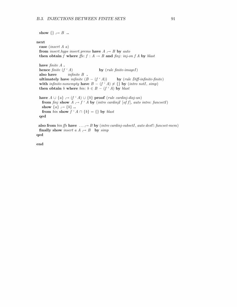
B.3. INJECTIONS BETWEEN FINITE SETS 91
show → B ..
nextcase (insert A a)from insert .hyps insert .prems have A → B by autothen obtain f where ffs : f : A → B and finj : inj-on f A by blast
have finite A .hence finite (f ‘ A) by (rule finite-imageI )also have infinite B .ultimately have infinite (B − (f ‘ A)) by (rule Diff-infinite-finite)with infinite-nonempty have B − (f ‘ A) 6= by (intro notI , simp)then obtain b where bin: b ∈ B − (f ‘ A) by blast
have A ∪ a → (f ‘ A) ∪ b proof (rule cardinj-disj-un)from finj show A → f ‘ A by (intro cardinjI [of f ], auto intro: funcsetI )show a → b ..from bin show f ‘ A ∩ b = by blast
qed
also from bin ffs have . . . → B by (intro cardinj-subsetI , auto dest !: funcset-mem)finally show insert a A → B by simp
qed
end

Appendix C
Finite Sums over AbelianMonoids
theory FiniteSum = CRing :
This extends the theory of finsums developed in CRing.thy and brings it upto speed with the theory of setsums.
Bound Syntax
syntax-finsum :: ′a ring ⇒ idt ⇒ ′b set ⇒ ′a ⇒ ′a (
∑ı-:-. - [0 , 51 , 10 ] 10 )
translations-finsum G i A f == finsum G (%i . f ) A
declare funcsetI [intro] funcset-mem [dest ]
declare (in abelian-monoid) finsum-cong [cong ]
lemmas subset-simps = subset-def Pi-def
Some Basic Properties
lemma (in abelian-group) finsum-diff1 :assumes fin: finite I
and ainI : a ∈ Iand fs : f ∈ I → carrier G
shows finsum G f (I − a) = finsum G f I f aproof −from ainI have I = I − a ∪ a by blasthence finsum G f I = finsum G f (I − a ∪ a) by (simp!)also have . . . = finsum G f (I − a) ⊕ finsum G f a by
(subst finsum-Un-disjoint , auto!)
92

93
also have . . . = finsum G f (I − a) ⊕ f a by (simp!add : subset-simps)
finally have finsum G f I f a = finsum G f (I − a) ⊕ f a f a by(simp add : minus-def )from this [symmetric] show finsum G f (I − a) = finsum G f I f a by
(simp! add : Pi-def minus-def a-assoc r-neg)qed
lemma inj-not-mem-image [intro,simp]:assumes inj : inj-on f A and sub: B ⊆ A and xmemA: x ∈ A and xnotB : x /∈
Bshows f x /∈ f ‘ Bby (simp! add : inj-on-def image-def , blast)
Reindexing
The following reindexing lemma should probably be in CRing.thy. It is anexpanded isar proof of the similar lemma setsum-reindex
lemma (in abelian-monoid) finsum-reindex :assumes all : finite B
inj-on f Bh : f ‘ B → carrier G
shows finsum G h (f ‘ B) = finsum G (h f ) Bproof (insert all , induct set : Finites)case emptyshow ?case by simp
nextcase (insert F x )show finsum G h (f ‘ insert x F ) = finsum G (h f ) (insert x F )proof −have indeq : finsum G h (f ‘ F ) = finsum G (h f ) F by (simp! add : subset-simps
inj-on-def image-def )
have f ‘ insert x F = insert (f x ) (f ‘ F ) by autohence finsum G h (f ‘ insert x F ) = finsum G h (insert (f x ) (f ‘ F )) by (simp!)also have . . . = h (f x ) ⊕ finsum G h (f ‘ F ) by (simp!
add : subset-simps)also from indeq have . . . = (h f ) x ⊕ finsum G (h f ) F by simpalso have . . . = finsum G (h f ) (insert x F ) by (simp!
add : subset-simps)finally show ?thesis .
qedqed
lemma (in abelian-monoid) finsum-reindex-id :assumes finite B inj-on f B f : B → carrier Gshows finsum G f B = finsum G id (f ‘ B)
by (rule finsum-reindex [of B f id , simplified image-id id-o, symmetric], auto! simp:

94 APPENDIX C. FINITE SUMS OVER ABELIAN MONOIDS
subset-simps)
Congruence Rules
lemma (in abelian-monoid) finsum-reindex-cong :assumes fin: finite A and inj : inj-on f A and hfs : h : B → carrier G
and cong : B = f ‘ A and restrict-eq :∧
i . i ∈ A =⇒ g i = h (f i)shows finsum G h B = finsum G g A
proof −from cong have finsum G h B = finsum G h (f ‘ A) by (simp only :)also have . . . = finsum G (h f ) A by (rule finsum-reindex ,
auto!)also have . . . = finsum G g A by (simp! add : subset-simps)finally show ?thesis .
qed
lemma (in abelian-group) finsum-reindex-cong ′:assumes fin: finite A and inj : inj-on f A and hfs : h : B → carrier G
and cong : B = f ‘ A and full-eq : g = h fshows finsum G h B = finsum G g A
by (rule finsum-reindex-cong , auto!)
Finite sums over Sigma domains
The following proofs are just lifted and adapted from the FiniteSet.thyproofs.
declare (in abelian-monoid) finsum-cong [cong del ]
lemma (in abelian-monoid) finsum-UN-disjoint :assumes all : finite I
(∀ i∈I . finite (A i))(∀ i∈I . ∀ j∈I . i 6= j −→ A i ∩ A j = )(∀ i∈I . f : (A i) → carrier G)
shows (∑
i :(UNION I A). f i) = (∑
i :I .∑
k :A i . f k)proof (insert all , induct set : Finites)case emptyshow ?case by simp
next case (insert F j )show (
∑i :(
⋃k∈insert j F A k). f i) = (
∑i :insert j F .
∑k :A i . f k)
proof −have (
∑i :(
⋃k∈insert j F A k). f i) = (
∑i :A j ∪ (
⋃k∈F A k). f i) by
simpalso have . . . = (
∑i :A j . f i) ⊕ (
∑i :(
⋃k∈F A k). f i) by (subst finsum-Un-disjoint ,
auto! simp: Pi-def )also have . . . = (
∑i :A j . f i) ⊕ (
∑i :F .
∑k :A i . f k) by (simp!)
also have . . . = (∑
i :insert j F .∑
k :A i . f k) by (subst finsum-insert)(auto!)
finally show ?thesis .

95
qedqed
lemma (in abelian-monoid) finsum-UN-disjoint-old :finite I =⇒ (∀ i∈I . finite (A i)) =⇒
(∀ i∈I . ∀ j∈I . i 6= j −→ A i ∩ A j = ) =⇒(∀ i∈I . f : (A i) → carrier G) =⇒finsum G f (UNION I A) = finsum G (%i . finsum G f (A i)) I
apply (induct set : Finites , simp, atomize)apply (subgoal-tac ALL i :F . x 6= i)prefer 2 apply blastapply (subgoal-tac A x Int UNION F A = )prefer 2 apply blastapply (subgoal-tac f : A x → carrier G)prefer 2 apply blastapply (subgoal-tac f : UNION F A → carrier G)prefer 2 apply blastapply (subgoal-tac (λi . finsum G f (A i)) : F → carrier G)prefer 2 apply (rule funcsetI , rule finsum-closed , blast , blast)apply (subgoal-tac finsum G f (A x ) ∈ carrier G)prefer 2 apply (rule finsum-closed , blast , blast)apply (simp add : finsum-Un-disjoint)done
lemma (in abelian-monoid) finsum-Union-disjoint :finite C =⇒ (∀A∈C . finite A) =⇒
(∀A∈C . ∀B∈C . A 6= B −→ A ∩ B = ) =⇒(∀A∈C . f : A → carrier G) =⇒
finsum G f (⋃
C ) = finsum G (finsum G f ) Capply (frule finsum-UN-disjoint [of C id f ])apply (unfold Union-def id-def , assumption+)done
lemma (in abelian-monoid) finsum-Sigma:finite A =⇒ ∀ x∈A. finite (B x ) =⇒ ∀ x∈A. ∀ y∈B x . f x y ∈ carrier G =⇒
(∑
x :A. (∑
y :B x . f x y)) =(∑
z :(Σ x∈A. B x ). f (fst z ) (snd z ))apply (subst Sigma-def )apply (subst finsum-UN-disjoint)apply assumptionapply (rule ballI )apply (drule-tac x = z in bspec, assumption)apply (subgoal-tac (UN y :(B z ). (z , y)) <= (%y . (z , y)) ‘ (B z ))apply (rule finite-surj )apply autoapply (rule finsum-cong , rule refl)apply (simp, rule funcsetI ) apply (rule finsum-closed , auto)apply (subst finsum-UN-disjoint)

96 APPENDIX C. FINITE SUMS OVER ABELIAN MONOIDS
apply (erule bspec, assumption)apply (auto)apply (rule finsum-cong , auto)done
lemma (in abelian-monoid) finsum-cartesian-product :finite A =⇒ finite B =⇒ ∀ x∈A.∀ y∈B . f x y ∈ carrier G =⇒
(∑
x :A. (∑
y :B . f x y)) =(∑
z :A × B . f (fst z ) (snd z ))by (erule finsum-Sigma, auto)
Sum Swapping
Sum swapping proofs. These are useful for reasonable reasoning about sumsover sums.
constdefspairswap :: ′a × ′b ⇒ ′b × ′apairswap z ≡ (snd z , fst z )
lemma pairswap-eq [iff ]: pairswap (a, b) = (b, a)by (simp add : pairswap-def )
lemma pairswap-inj-onI [intro]: inj-on pairswap ABby (rule inj-onI , auto)
lemma pairswap-imageI [iff ]: pairswap ‘ (A × B) = B × Aproof (auto)fix a b assume a ∈ A b ∈ Bhence (a,b) ∈ A × B ..hence pairswap (a,b) ∈ pairswap ‘ (A × B) by blastthus (b, a) ∈ pairswap ‘ (A × B) by simp
qed
lemma setsum-setsum-swap:assumes finite A finite Bshows (
∑a:A.
∑b:B . f a b ) = (
∑b:B .
∑a:A. f a b)
proof −have (
∑a:A.
∑b:B . f a b ) = (
∑z∈A × B . f (fst z ) (snd z )) by (rule
setsum-cartesian-product)also have . . . = (
∑z∈A × B . split f z ) by (simp add :
split-def )also have . . . = (
∑z∈pairswap ‘ (B × A). split f z ) by simp
also have . . . = (∑
z∈B × A. ((split f ) pairswap) z ) by (rulesetsum-reindex )
(auto! intro:finite-cartesian-product)also have . . . = (
∑z∈B × A. f (snd z ) (fst z )) by (simp add :
split-def pairswap-def )also have . . . = (
∑b:B .
∑a:A. f a b) by (rule

97
setsum-cartesian-product [symmetric])finally show ?thesis .
qed
lemma (in abelian-monoid) finsum-finsum-swap:assumes finite A finite B ∀ a∈A.∀ b∈B . f a b ∈ carrier Gshows (
∑a:A.
∑b:B . f a b ) = (
∑b:B .
∑a:A. f a b)
proof −have (
∑a:A.
∑b:B . f a b ) = (
∑z :A × B . f (fst z ) (snd z )) by (rule
finsum-cartesian-product)also have . . . = (
∑z :A × B . split f z ) by (simp add :
split-def )also have . . . = (
∑z :pairswap ‘ (B × A). split f z ) by simp
also have . . . = (∑
z :B × A. ((split f ) pairswap) z ) by (rulefinsum-reindex )
(auto! intro:finite-cartesian-product)also have . . . = (
∑z :B × A. f (snd z ) (fst z )) by (simp
add : split-def pairswap-def )also have . . . = (
∑b:B .
∑a:A. f a b) by (rule
finsum-cartesian-product [symmetric], auto!)finally show ?thesis .
qed
lemma (in abelian-group) finsum-minus-f [simp]:assumes all : finite A f : A → carrier Gshows (
∑a:A. f a) = (
∑a:A. f a)
proof (insert all , induct set : Finites)case emptyshow ?case by simp
next case (insert F x )have (
∑a:insert x F . f a) = f x ⊕ (
∑a:F . f a) by (simp! add : Pi-def )
also have . . . = f x ⊕ (∑
a:F . f a) by (simp! add : Pi-def )also have . . . = (f x ⊕ (
∑a:F . f a)) by (simp! add : minus-add Pi-def )
also have . . . = (∑
a:insert x F . f a) by (simp! add : Pi-def )finally show ?case .
qed
lemma (in abelian-group) finsum-diff-f :assumes finite A f : A → carrier G g : A → carrier Gshows (
∑a:A. f a g a) = (
∑a:A. f a) (
∑a:A. g a)
by (simp! cong : finsum-cong add : minus-def finsum-addf add : Pi-def )
declare funcsetI [rule del ] funcset-mem [rule del ]
end

Appendix D
Real Vector Spaces
theory VectorSpace = MiscPrelim + CRing + FiniteSum + CardInj :
D.1 Real Vector Spaces
Mathematically, we abstractly define the category of vector spaces as abeliangroups with a real scalar product operation. This theory file develops thecalculational properties needed for evaluation of expressions involving thisproduct, including some useful factoring properties over the finite summa-tion operation.
In Ballarin’s CRing theory, the locale abelian-group is defined over recordsof type ring, ignoring the multiplicative fields. Having random unused fieldsin the algebraic structure is not exactly appealing, but is necessitated if wewish to inherit the extensive set of calculational lemmas that he has provenabout abelian groups.
D.1.1 Definitions
record ′a realvectorspace-t = ′a ring +rprod :: [real , ′a] ⇒ ′a (infixr ·ı 70 )
locale realvectorspace = abelian-group V +assumes rprod-closed [simp,intro]: x ∈ carrier V =⇒ a · x ∈ carrier V
and add-rprod-distrib1 : [[x ∈ carrier V ; y ∈ carrier V ]] =⇒ a · (x ⊕ y) = a· x ⊕ a · y
and add-rprod-distrib2 : x ∈ carrier V =⇒ (a + b) · x = a · x ⊕ b · xand rprod-assoc: x ∈ carrier V =⇒ (a ∗ b) · x = a · (b · x )and rprod-1 [simp]: x ∈ carrier V =⇒ 1 · x = xand negate-eq1 : x ∈ carrier V =⇒ x = (− 1 ) · x
lemma (in realvectorspace) realvectorspace-selfI [intro]: realvectorspace Vby (intro realvectorspace.intro)
98

D.1. REAL VECTOR SPACES 99
D.1.2 Basic Properties
These lemmas follow the development in the Hahn Banach VectorSpace.thyfile. This is the primary example of desired “reuse” that involved manualparaphrasing. From a systems programming point of view, it is unfair toexpect that Wenzel’s axiomatic type class based vector space theory wouldbe compatible with Ballarin’s record-based algebraic theories. From a math-ematical point of view however, we would hope that a “VectorSpace.thy”would be relatable to a “CRing.thy” no matter what.
We suppress most of these calculational properties in the interest of rainfor-est conservation.
D.1.3 Finite Sums in Real Vector Spaces
The following lemmas are specifically for finite sums over vectorspaces (ie.they make use of the scalar product.) Note that there are two different finitesummation operations in use here: the finsum operator, defined over Bal-larin’s abelian groups, and the setsum operator, defined over types of classabelian group. Although they are presented using the same symbol Σ, infact, they rely on two completely separate but parallel theory developments,because of the difference in underlying set representation.
lemma (in realvectorspace) finsum-rprod-assoc [simp]:assumes B ⊆ carrier Vshows finsum V (λu. (a u ∗ b u) · u) B = finsum V (λu. a u · b u · u) B
by (simp! cong : finsum-cong add : rvs-simprules subset-simps)
— Both summation signs below are the finsum operator.lemma (in realvectorspace) finsum-l-factor :assumes all : finite I v : I → carrier Vshows (
∑i :I . a · v i) = a · (
∑i :I . v i)
proof (insert all , induct set : Finites)case emptyshow ?case by simp
next case (insert F x )hence indeq : (
∑i :F . a · v i) = a · finsum V v F by (auto)
— The proof of this theorem demonstrates the complexity of conditional simplifi-cation in the presence of set membership conditions, prior to the introduction of thepredicate subtyper. Notice how many lines amount to single step rewriting usingthe subst tactic followed by a call to a classical reasoner to solve the subset con-ditions. The level of detail in the calculation is excruciating and the justificationstook a long time to figure out.

100 APPENDIX D. REAL VECTOR SPACES
show (∑
i :insert x F . a · v i) = a · finsum V v (insert x F )proof −
have (∑
i :insert x F . a · v i) = a · v x ⊕ (∑
i :F . a · v i) by (substfinsum-insert , auto!)
also from indeq have . . . = a · v x ⊕ a · (∑
i :F . v i) by simpalso have . . . = a · (v x ⊕ (
∑i :F . v i)) by (subst
add-rprod-distrib1 , auto! simp: Pi-def )also have . . . = a · (
∑i :insert x F . v i) by (subst
finsum-insert , auto!)finally show ?thesis .
qedqed
— The right hand side summation is actually a setsum while the left hand sidesummation is a finsum.lemma (in realvectorspace) finsum-r-factor :assumes all : finite A v ∈ carrier Vshows (
∑a:A. f a · v) = (
∑a:A. f a) · v
— We suppress the proof because it is similar to the previous.end
D.2 Subspaces
theory Subspace = VectorSpace:
D.2.1 Definition
A non-empty subset U of a vector space V is a subspace of V, iff U is closedunder addition and scalar multiplication.
In order to have the write vector space parameters available when reasoninginside of the subset U , we have defined the subspace parameter as a fullvectorspace record and required that the operation fields be the same asthose in the superspace V . This definition does not assert that U is a vectorspace itself, which we prove later, only that it has the representation ofa vector space. Also, the equality of operator assumptions are somewhatirritating to work with because we must manually lift expressions back andforth across that equality.
locale subspace = var U + realvectorspace V +assumes non-empty [simp, intro]: carrier U 6= and subset [simp, intro]: carrier U ⊆ carrier Vand add-closed [simp, intro]: [[x ∈ carrier U ; y ∈ carrier U ]] =⇒ x ⊕ y ∈
carrier Uand rprod-closed [simp,intro]: x ∈ carrier U =⇒ a · x ∈ carrier U
assumes same-add [simp]: add U = add V

D.2. SUBSPACES 101
and same-zero [simp]: zero U = zero Vand same-rprod [simp]: rprod U = rprod V
syntax (symbols)
subspace :: ′a realvectorspace-t ⇒ ′a realvectorspace-t ⇒ bool (infix E 50 )
We suppress the development of the properties of subspaces and the subspacerelation (eg. that it is transitive and reflexive).
D.2.2 Basic Properties
lemma subspace-subset [elim]: subspace U V =⇒ carrier U ⊆ carrier Vby (rule subspace.subset)
lemma (in subspace) subsetD [simp,intro]: x ∈ carrier U =⇒ x ∈ carrier Vusing subset by blast
lemma subspaceD [elim]: U E V =⇒ x ∈ carrier U =⇒ x ∈ carrier Vby (rule subspace.subsetD)
lemma rev-subspaceD [elim? ]: x ∈ carrier U =⇒ U E V =⇒ x ∈ carrier Vby (rule subspace.subsetD)
lemma (in subspace) minus-closed [simp,intro]: x ∈ carrier U =⇒ x ∈ carrierUproof −assume x ∈ carrier Uhence −1 · x ∈ carrier U ..thus x ∈ carrier U by (simp! add : negate-eq1 )
qed
lemma (in subspace) diff-closed [simp,intro]:shows x ∈ carrier U =⇒ y ∈ carrier U =⇒ x y ∈ carrier U
by (simp add : minus-def )
Similar as for linear spaces, the existence of the zero element in every sub-space follows from the non-emptiness of the carrier set and by vector spacelaws.
lemma (in subspace) zero [intro]:shows 0 ∈ carrier U
proof −have carrier U 6= ..then obtain x where x : x ∈ carrier U by blasthence x ∈ carrier V .. hence 0 = x x by simpalso have ... ∈ carrier U by (rule U-V .diff-closed)finally show ?thesis .
qed

102 APPENDIX D. REAL VECTOR SPACES
lemma (in subspace) neg-closed [simp,intro]:shows x ∈ carrier U =⇒ x ∈ carrier U
by (simp add : negate-eq1 )
Further derived laws: every subspace is a vector space.
lemma (in subspace) subspace-inv-unique:assumes x ∈ carrier Ushows ∃ ! y . y ∈ carrier U ∧ x ⊕ y = 0 ∧ y ⊕ x = 0
proofshow ∃ y . y ∈ carrier U ∧ x ⊕ y = 0 ∧ y ⊕ x = 0 proof (rule exI , intro conjI )
show x ∈ carrier U ..show x ⊕ x = 0 by (auto! intro!: l-neg)show x ⊕ x = 0 by (auto! intro!: r-neg)
qed
fix y y ′ assume y ∈ carrier U ∧ x ⊕ y = 0 ∧ y ⊕ x = 0 y ′ ∈ carrier U ∧ x⊕ y ′ = 0 ∧ y ′ ⊕ x = 0show y = y ′
proof −have xyy ′: x ∈ carrier V y ∈ carrier V y ′ ∈ carrier V by (auto!)have x ⊕ y ′ = 0 by (auto!)also have x ⊕ y = 0 by (auto!)finally have x ⊕ y = x ⊕ y ′ .thus y = y ′ using xyy ′ by (simp)
qedqed
lemma (in subspace) lift-a-inv [iff ]:assumes [intro,simp]: x ∈ carrier Ushows a-inv U x = a-inv V x
proof −have a-inv U x = (THE y . y ∈ carrier U ∧ x ⊕ y = 0 ∧ y ⊕ x = 0) by (simp
add : a-inv-def m-inv-def )also have . . . = xproof (rule the1-equality)show ∃ !y . y ∈ carrier U ∧ x ⊕ y = 0 ∧ y ⊕ x = 0 by (rule subspace-inv-unique)show x ∈ carrier U ∧ x ⊕ x = 0 ∧ x ⊕ x = 0 by (auto intro: l-neg
r-neg)qedfinally show ?thesis .
qed
lemma (in subspace) realvectorspace [iff ]:shows realvectorspace U
— Proof suppressed.
lemma (in realvectorspace) subset-subspaceI :fixes Uassumes nempty : U 6=

D.2. SUBSPACES 103
and sub: U ⊆ carrier Vand add-cl :
∧x y . [[ x ∈ U ; y ∈ U ]] =⇒ x ⊕ y ∈ U
and rp-cl :∧
x a. x ∈ U =⇒ a · x ∈ Ushows subspace (V (|carrier := U |)) V
proof (intro subspace.intro subspace-axioms .intro)show carrier (V (|carrier := U |)) 6= by simpshow carrier (V (|carrier := U |)) ⊆ carrier V by simpfix a::real fix x y assume assm: x ∈ carrier (V (|carrier := U |)) y ∈ carrier
(V (|carrier := U |))hence xy : x ∈ U y ∈ U by autoshow x ⊕ y ∈ carrier (V (|carrier := U |)) using add-cl by (simp add : xy)show a · x ∈ carrier (V (|carrier := U |)) using rp-cl by (simp add : xy)
qed auto
The subspace relation is reflexive.
lemma (in realvectorspace) subspace-refl [intro]: V E Vproof (intro subspace.intro subspace-axioms .intro)show carrier V 6= ..show carrier V ⊆ carrier V ..fix x y assume x : x ∈ carrier V and y : y ∈ carrier Vfix a :: realfrom x y show x ⊕ y ∈ carrier V by simpfrom x show a · x ∈ carrier V by simp
qed auto
The subspace relation is transitive.
lemma (in realvectorspace) subspace-trans [trans ]:fixes W (structure)shows U E W =⇒ W E V =⇒ U E V
proof (intro subspace.intro subspace-axioms .intro)assume uw : U E W and wv : W E Vfrom uw show carrier U 6= by (rule subspace.non-empty)show carrier U ⊆ carrier Vproof −from uw have carrier U ⊆ carrier W by (rule subspace.subset)also from wv have carrier W ⊆ carrier V by (rule subspace.subset)finally show ?thesis .
qed
from uw wv show add U = op ⊕ by (simp add : subspace.same-add)from uw wv show rprod U = op · by (simp add : subspace.same-rprod)from uw wv show zero U = 0 by (simp add : subspace.same-zero)
fix x y assume x : x ∈ carrier U and y : y ∈ carrier Ufrom uw and x y have x ⊕2 y ∈ carrier U by (rule subspace.add-closed)with wv show x ⊕ y ∈ carrier U by (simp add : subspace.same-add)from uw and x have
∧a. a ·2 x ∈ carrier U by (rule subspace.rprod-closed)
with wv show∧
a. a · x ∈ carrier U by (simp add : subspace.same-rprod)

104 APPENDIX D. REAL VECTOR SPACES
qed
end

Appendix E
Linear Combinations
theory LinearComb = VectorSpace + Subspace:
The heart of our vector space theory develops the notions of linear com-binations, linear dependence, spanning sets and basis sets. These are allfundamental to reasoning in vector spaces.
In normal mathematics practice, indexed sequences and summations areinterchangeable with statements about finite sets and finite sums over them.This is not so easy in a formal setting and we have opted to develop thetheory in an index-free manner, which makes some of the expressions reada bit unusally. This is a readability-complexity trade-off that we agonizedover long and hard before deciding to drop our beloved indices.
E.1 Linear Combination Operation
E.1.1 The base Predicate
A (finite) linear combination in a vector space V is given by a finite subsetB of carrier V and a coefficient map on that set a ∈ B → IR. Thus, thelinear combination represented is simply
∑w :W . (a w) · w. We define a
predicate lc-base to collect the conditions on the set B for this product tobe well defined as a linear combination.
constdefslc-base :: ( ′a, ′b) realvectorspace-t-scheme ⇒ ′a set ⇒ bool (baseı)lc-base V B ≡ (B ⊆ carrier V ∧ finite B)
lemma (in realvectorspace) lc-baseI [intro]: [[finite B ; B ⊆ carrier V ]] =⇒ base Bby (simp add : lc-base-def )
lemma (in realvectorspace) lc-base-finiteD [simp,dest ]: base B =⇒ finite Bby (simp add : lc-base-def )
105

106 APPENDIX E. LINEAR COMBINATIONS
lemma (in realvectorspace) lc-base-subcarrierD [simp,dest ]: base B =⇒ B ⊆ car-rier Vby (simp only : lc-base-def )
lemma (in realvectorspace) lc-base-mem-carrier [simp]: base B =⇒ ∀ x∈B . x ∈carrier Vby (auto)
lemma (in realvectorspace) lc-base-finsum-closed [simp]:[[base A; ∀ a∈A. f a ∈ carrier V ]] =⇒ finsum V f A ∈ carrier Vby (auto intro!: funcsetI finsum-closed)
lemma (in realvectorspace) lc-base-emptyI [simp,intro]: base by (auto)
lemma (in realvectorspace) lc-base-insertI [simp,intro]: [[base A;x ∈ carrier V ]]=⇒ base (insert x A)by (auto)
lemma (in realvectorspace) lc-base-unionI [simp,intro]: [[ base A; base B ]] =⇒base (A ∪ B)by (auto)
lemma (in realvectorspace) lc-base-interI [simp,intro]: base A =⇒ base (A ∩ B)by (auto)
lemma (in realvectorspace) lc-base-diffI [simp,intro]: base A =⇒ base (A − B)by (auto)
lemma (in realvectorspace) lc-base-subD [elim]: [[base A; B ⊆ A]] =⇒ base Bby (auto intro!: lc-baseI elim: finite-subset)
lemma (in realvectorspace) lc-base-fin-UN-I [simp,intro]:assumes finite I ∀ i∈I . base (A i)shows base (
⋃i∈IA i)
proofshow (
⋃i∈I A i) ⊆ carrier V by (simp! add : UN-subset-iff )
show finite (⋃
i∈I A i) by (auto! intro!: finite-UN-I )qed
E.1.2 The Linear Combination Op
The linear combination sum,∑
w :W . (a w) · w, arises regularly enoughthat we define a product symbol · to represent it. We then develop a com-plete set of calculational/simplifier properties for this operation.
constdefslc-prod :: ( ′a, ′b) realvectorspace-t-scheme ⇒ ( ′a ⇒ real) ⇒ ′a set => ′a (infix
·ı 70 )lc-prod V a B ≡ finsum V (λv . rprod V (a v) v) B
lemma (in realvectorspace) lc-prod-mem-carrier [simp,intro]:base B =⇒ a · B ∈ carrier Vby (simp add : lc-prod-def )

E.1. LINEAR COMBINATION OPERATION 107
Simplifier Rules
lemmas (in realvectorspace) lc-prod-value = lc-prod-def
lemma (in realvectorspace) lc-prod-empty [simp]: a · = 0by (simp add : lc-prod-value)
lemma (in realvectorspace) lc-prod-zero [simp]:[[ base A; ∀ x ∈ A. a x = 0 ]] =⇒ a · A = 0by (simp cong : finsum-cong add : lc-prod-value Pi-def )
lemma (in realvectorspace) lc-prod-cong [cong ]:[[ A = B ; (base B) = True;
∧i . i ∈ B =⇒ a i = b i ]] =⇒ a · A = b · B
by (auto simp add : lc-prod-value intro!: finsum-cong funcsetI )
Combination Rules
The following lemmas allow us to combine linear combinations in variousways to get new linear combinations.
lemma (in realvectorspace) lc-prod-Un-Int :assumes base A base Bshows a · (A ∪ B) ⊕ a · (A ∩ B) = a · A ⊕ a · Bby (simp! add : lc-prod-value finsum-Un-Int Pi-def )
lemma (in realvectorspace) lc-prod-Un-disjoint :assumes base A base B A ∩ B = shows a · (A ∪ B) = a · A ⊕ a · Bby (simp! add : lc-prod-Un-Int [symmetric])
lemma (in realvectorspace) lc-prod-insert [simp,intro]:assumes base A x ∈ carrier V x /∈ Ashows a · (insert x A) = a x · x ⊕ a · Aby (simp! add : lc-prod-value Pi-def )
lemma (in realvectorspace) lc-prod-diff :assumes base Ashows a · (A − B) = a · A a · (A ∩ B)
proof −have A = (A − B) ∪ (A ∩ B) by blastmoreover have (A − B) ∩ (A ∩ B) = by blastultimately have a · A = a · (A − B) ⊕ a · (A ∩ B) by (simp! add :
lc-prod-Un-disjoint [symmetric])hence a · A a · (A ∩ B) = a · (A − B) ⊕ a · (A ∩ B) a · (A ∩ B) by
(simp!)from this [symmetric] show a · (A − B) = a · A a · (A ∩ B) by (simp! add :
rvs-simprules minus-def )qed
lemma (in realvectorspace) lc-prod-zero-reduce:

108 APPENDIX E. LINEAR COMBINATIONS
assumes base A B ⊆ A ∀ u∈(A − B). a u = 0shows a · A = a · B
proof −presume base Bhave B = A ∩ B by (blast !)hence a · (A − B) = a · A a · B by (simp! only : lc-prod-diff )hence 0 = a · A a · B by (simp!)hence 0 ⊕ a · B = a · A a · B ⊕ a · B by (simp!)hence a · B = a · A by (simp! add : a-assoc l-neg minus-def )thus ?thesis ..
nextshow base B by (rule lc-base-subD)
qed
lemma (in realvectorspace) lc-prod-l-distrib: base A =⇒ (λv . a v + b v) · A = a· A ⊕ b · Aby (simp cong : finsum-cong add : lc-prod-value finsum-addf rprod-distrib Pi-def )
lemma (in realvectorspace) lc-prod-lm-distrib: base A =⇒ (λv . a v − b v) · A =a · A b · Aby (simp cong : finsum-cong add : lc-prod-value finsum-addf rprod-distrib minus-def
Pi-def )
lemma (in realvectorspace) lc-prod-factor : base A =⇒ (λv . a ∗ f v) · A = a · f ·Aby (simp cong : finsum-cong add : lc-prod-value finsum-l-factor rprod-assoc Pi-def )
The Sum of Linear Combinations is a Linear Combination
This is a very important property. When we add a · A ⊕ b · B, we canre-represent this as c · C where C is the union of A and B and the coefficientfunction c is given by the sum of a and b where A and B intersect, but byjust a or b where they do not.
constdefszerofun :: ′a ⇒ realzerofun x ≡ 0
declare zerofun-def [simp]
lemma (in realvectorspace) lc-prod-sum:assumes base A base Bshows a · A ⊕ b · B = (λv . (zerofun(a|A)) v + (zerofun(b|B)) v) · (A ∪ B)
(is ?lhs = ?rhs)proof −have ?rhs = (zerofun(a|A)) · (A ∪ B) ⊕ (zerofun(b|B)) · (A ∪ B) by (simp!
add : lc-prod-l-distrib)also have . . . = (zerofun(a|A)) · A ⊕ (zerofun(b|B)) · (A ∪ B)

E.1. LINEAR COMBINATION OPERATION 109
by (subst lc-prod-zero-reduce [of - A (zerofun(a|A))], auto!)also have . . . = (zerofun(a|A)) · A ⊕ (zerofun(b|B)) · B
by (subst lc-prod-zero-reduce [of - B (zerofun(b|B))], auto!)also have . . . = a · A ⊕ b · B by (simp!)finally show ?thesis ..
qed
The above lemma is constructive but a bit long to use. The following lemmais easier if we need to only show existence of the sum.
lemma (in realvectorspace) lc-prod-sum-ex :assumes base A base Bshows ∃ c. a · A ⊕ b · B = c · (A ∪ B)by (rule exI , rule lc-prod-sum)
lemma (in realvectorspace) lc-prod-finsum-ex :assumes all : finite I ∀ i∈I . base (A i)shows ∃ c. (
∑i :I . a i · A i) = c · (
⋃i∈I A i)
proof (insert all , induct set : Finites)case emptyshow ?case by simp
nextcase (insert F j )from insert .prems have ∀ i∈insert j F . base (A i) .hence ∀ i∈F . base (A i) by blast
with insert .hyps have ∃ c. (∑
i :F . a i · A i) = c · (⋃
i∈F A i) by blastthen obtain c where cval : (
∑i :F . a i · A i) = c · (
⋃i∈F A i) by blast
from lc-prod-sum-ex have ∃ d . a j · A j ⊕ c · (⋃
i∈F A i) = d · (A j ∪ (⋃
i∈F
A i)) by (auto!)then obtain d where dval : a j · A j ⊕ c · (
⋃i∈F A i) = d · (A j ∪ (
⋃i∈F
A i)) by (blast)
have (∑
i :insert j F . a i · A i) = a j · A j ⊕ (∑
i :F . a i · A i) by (simp! add :Pi-def )also from cval have . . . = a j · A j ⊕ c · (
⋃i∈F A i) by
simpalso from dval have . . . = d · (A j ∪ (
⋃i∈F A i)) by
simpalso have . . . = d · (
⋃i∈insert j F A i) by
(simp!)finally have (
∑i :insert j F . a i · A i) = d · (
⋃i∈insert j F A i) .
thus ∃ c. (∑
i :insert j F . a i · A i) = c · UNION (insert j F ) A by autoqed

110 APPENDIX E. LINEAR COMBINATIONS
E.1.3 Nontrivial Linear Combinations
A linear combination is nontrivial if at least one of the coefficients in it isnonzero.
constdefsnontrivial :: ( ′a ⇒ real) ⇒ ′a set ⇒ boolnontrivial a W ≡ ∃w ∈ W . a w 6= 0
lemma nontrivialI [intro]: [[ w ∈ W ; a w 6= 0 ]] =⇒ nontrivial a Wby (auto simp add : nontrivial-def )
lemma nontrivialE [elim]: [[nontrivial a W ;∧
w . [[w ∈ W ; a w 6= 0 ]] =⇒ R]] =⇒Rby (auto simp add : nontrivial-def )
lemma nontrivial-nonemptyD [dest ]: nontrivial a W =⇒ W 6= by blast
lemma nontrivial-zero-reduce:assumes nt : nontrivial a A and sub: B ⊆ A
and zero: ∀ u∈(A − B). a u = 0shows nontrivial a B
proof −from nt obtain i where i ∈ A and nz : a i 6= 0 by blastmoreover with zero have i /∈ A − B by blastultimately have i ∈ B by blastthus ?thesis ..
qed
E.2 Linear Dependence
We use a general definition of linear dependence that holds for infinite setsas well as the finite sets we usually think about. A set of vectors A islinearly dependent if there exists a finite subset of A that can be nontriv-ially combined to get 0. A set is linearly independent if it is not linearlydependent.
In Isabelle, we define linear dependence as a predicate on sets but definelinear independence as a syntax translation indicating the negation of lineardependence. This technique follows the example given by the “predicate”infinite, which is actually just syntax for ¬ finite.
E.2.1 Definition
constdefslineardependent :: ( ′a, ′m) realvectorspace-t-scheme ⇒ ′a set ⇒ bool (lineardepı)lineardependent V A ≡ A ⊆ carrier V
∧ (∃ B a. B ⊆ A ∧ lc-base V B ∧ nontrivial a B ∧ lc-prod V aB = (zero V ))

E.2. LINEAR DEPENDENCE 111
syntaxlinearindependent :: ( ′a, ′m) realvectorspace-t-scheme ⇒ ′a set ⇒ bool (linearindı
-)
translationslinearindependent V A ¬ lineardependent V A
lemma (in realvectorspace) lineardepI [intro]:assumes A ⊆ carrier V
and B ⊆ Aand base Band nontrivial a Band a · B = 0
shows lineardep Aby (unfold lineardependent-def , intro conjI exI )
lemma (in realvectorspace) lineardep-subcarrierD [dest ]: lineardep A =⇒ A ⊆ car-rier Vby (auto simp add : lineardependent-def )
lemma (in realvectorspace) lineardep-finite-baseD [dest ]: lineardep A =⇒ finite A=⇒ base Aby (auto)
lemma (in realvectorspace) lineardep-zerocomboD [dest ]:lineardep A =⇒ ∃B a. B ⊆ A ∧ base B ∧ nontrivial a B ∧ a · B = 0
by (auto simp add : lineardependent-def )
E.2.2 Basic Properties
lemma (in realvectorspace) empty-linearindI [intro]: linearind proofassume lineardep hence ∃B a. B ⊆ ∧ base B ∧ nontrivial a B ∧ a · B = 0 ..then obtain B a where B = nontrivial a B by blastwith nontrivial-nonemptyD show False by blast
qed
lemma (in realvectorspace) singleton-linearindI [intro]:assumes assms : v ∈ carrier V v 6= 0shows linearind v
proofassume lineardep vhence ∃B a. B ⊆ v ∧ base B ∧ nontrivial a B ∧ a · B = 0 ..then obtain B a where sub: B ⊆ v and base: base B and nt : nontrivial a
B and lc: a · B = 0 by blast
from nt have B 6= ..

112 APPENDIX E. LINEAR COMBINATIONS
with sub have [simp]: B = v by blasthence a · B = a v · v using base by (simp add : lc-prod-value)hence 0 = a v · v using lc by simpwith assms have a v = 0 by (simp add : rprod-zero-uniq)moreover from nt [simplified ] have a v 6= 0 by (blast)ultimately show False by contradiction
qed
lemma (in realvectorspace) zero-lineardepI [intro? ]:assumes 0 ∈ A A ⊆ carrier Vshows lineardep A
proofshow base 0 by autoshow 0 ⊆ A by (blast !)show nontrivial (λu. 1 ) 0 by auto
show (λu. 1 ) · 0 = 0 by (simp add : lc-prod-value)qed
lemma (in realvectorspace) sup-lineardepI [intro? ]:assumes sup: A ⊆ B
and subcar : B ⊆ carrier Vand ld : lineardep A
shows lineardep Bproof −from ld [THEN lineardep-zerocomboD ]obtain C a where CA: C ⊆ A and ntlc: base C nontrivial a C a · C = 0 by
blast
from CA sup have C ⊆ B by blastwith - show lineardep B by (rule lineardepI )
qed
lemma (in realvectorspace) sub-linearindI [intro? ]:assumes sub: A ⊆ B
and subcar : B ⊆ carrier Vand lid : linearind B
shows linearind Aproof (rule contrapos-nn)assume lineardep A with - - show lineardep B ..
qed
We prove two versions of the lemma showing that a linearly dependent sethas a vector in it that can be solved for in terms of the other vectors. Thesecond is this exact statement, and the first allows us to specify a linearlyindependent subset I of our linearly dependent set A and state that thesolved for vector comes from A - I.
lemma (in realvectorspace) lineardep-sub-solve:assumes ld-A: lineardep A

E.2. LINEAR DEPENDENCE 113
and A-nz : A 6= 0and IsubA: I ⊆ Aand li-I : linearind I
shows ∃ a v U . U ⊆ A ∧ v ∈ A − I − U ∧ base U ∧ a · U = vproof (cases)assume 0 ∈ Awith A-nz obtain v where vinA: v ∈ A and vnz : v 6= 0 by blast
show ∃ a v U . U ⊆ A ∧ v ∈ A − I − U ∧ base U ∧ a · U = vproof (intro exI conjI )from ld-A have A ⊆ carrier V ..with vinA have [simp]: v ∈ carrier V by blast
show v ⊆ A using vinA by auto
have 0 /∈ I proofassume 0 ∈ Ihence lineardep I by (rule zero-lineardepI , auto!)thus False by contradiction
qedthus 0 ∈ A − I − v by (blast !)
show (λu. 0 ) · v = 0 by (simp add : lc-prod-value)show base v by (auto)
qed
nextassume 0 /∈ A
from ld-A have [intro]: A ⊆ carrier V ..with IsubA have Isubcar : I ⊆ carrier V by blast
— First pick a nontrivial combo forming zerofrom ld-A [THEN lineardep-zerocomboD ] obtain B bwhere BsubA: B ⊆ Aand baseB : base Band nt-bB : nontrivial b Band b-B-z : b · B = 0
by blast
have ∃ w . w ∈ B − I ∧ b w 6= 0proof (rule classical)assume ¬ (∃w . w ∈ B − I ∧ b w 6= 0 )hence zeros : ∀w ∈ B − (B ∩ I ). b w = 0 by blast
have B ∩ I ⊆ I by blastfrom this Isubcar have li-BI : linearind (B ∩ I ) using li-I by (rule sub-linearindI )
— BUT

114 APPENDIX E. LINEAR COMBINATIONS
also have ld-BI : lineardep (B ∩ I ) prooffrom zeros baseB have b · B = b · (B∩I ) by (auto intro!: lc-prod-zero-reduce)with b-B-z show b · (B∩I ) = 0 by simp
from nt-bB - zeros show nontrivial b (B ∩ I ) by (rule nontrivial-zero-reduce,auto)
qed (auto!)
ultimately show ?thesis by contradictionqed
then obtain vwhere vinBmI : v ∈ B − I and bvnz : b v 6= 0by blast
from vinBmI have vinB [intro,simp]: v ∈ B by blast
show ∃ a v U . U ⊆ A ∧ v ∈ A − I − U ∧ base U ∧ a · U = vproof (intro exI conjI )from BsubA show B − v ⊆ A by blast
show vinset : v ∈ A − I − (B − v) prooffrom vinBmI BsubA show v ∈ A − I by blastshow v /∈ B − v by blast
qed
show base (B − v) ..
show (λu. (− 1 / b v ∗ b u)) · (B − v) = v (is ?c · (B − v) = v)proof −
have is-z : (λu. (− 1 / b v ∗ b u)) · B = 0 by (simp! only :lc-prod-factor rprod-zero-right)
from vinB have Bvabsorb: v = B∩v byblast
hence ?c · (B − v) = ?c · B ?c · v by(simp! only : lc-prod-diff )
also from is-z have . . . = 0 (λu.(− 1 / b v ∗ b u)) · v bysimp
also have . . . = 0 (− b v / b v) · v by (simp!add : lc-prod-value)
also have . . . = v by (simp! add :negate-eq2a minus-def )
finally show ?thesis .qed
qedqed
corollary (in realvectorspace) lineardep-solve:

E.3. LINEAR SPAN 115
assumes all : lineardep A A 6= 0shows ∃ a v U . U ⊆ A ∧ v ∈ A − U ∧ base U ∧ a · U = v
proof −from all have ∃ a v U . U ⊆ A ∧ v ∈ A − − U ∧ base U ∧ a · U = vby (rule lineardep-sub-solve, auto intro!: empty-linearindI )
thus ?thesis by blastqed
corollary (in realvectorspace) finite-lineardep-solve:assumes ld : lineardep A and finite: finite Ashows ∃ v vc. v ∈ A ∧ vc · (A − v) = v
proof (cases A = 0)assume nz : A 6= 0show ?thesis proof −
from ld nz have ∃ a v U . U ⊆ A ∧ v ∈ A − U ∧ base U ∧ a · U = v by(rule lineardep-solve)
then obtain a v U where UsubA: U ⊆ A and vinAU : v ∈ A − Uand baseU : base U and aUval : a · U = v by blast
show ∃ v vc. v ∈ A ∧ vc · (A − v) = vproof (intro exI conjI )from vinAU show v ∈ A by blastlet ?vc = zerofun(a|U )show ?vc · (A − v) = v proof −have base A by (rule lineardep-finite-baseD)hence base (A − v) ..hence ?vc · (A − v) = ?vc · U by (rule lc-prod-zero-reduce, insert UsubA
vinAU , auto)also from baseU have . . . = a · U by (simp add : lc-prod-value cong :
finsum-cong)also from aUval have . . . = v by simpfinally show ?thesis .
qedqed
qed
nextassume z : A = 0show ?thesis proof (intro exI conjI )from z show 0 ∈ A by blastfrom z show zerofun · (A − 0) = 0 by simp
qedqed
E.3 Linear Span
The span of a generating set A is the closure of A under finite linear com-bination. This definition requires the use of an existential finite subset of Afor each linear combination to be based on. A simpler definition is available

116 APPENDIX E. LINEAR COMBINATIONS
of we only consider the spanning sets of finite sets, because then we cansimply take that finite subset to be the set itself.
We use the more general definition and then prove the simplified statementfor finite A.
E.3.1 Definition
constdefsspan-set :: ( ′a, ′m) realvectorspace-t-scheme ⇒ ′a set ⇒ ′a set (spanı)span-set V A ≡ v . ∃ a W . W ⊆ A ∧ lc-base V W ∧ lc-prod V a W = v
lemma (in realvectorspace) mem-spanD [dest ]:assumes v ∈ span Ashows ∃ a W . W ⊆ A ∧ base W ∧ a · W = vby (auto! simp: span-set-def )
lemma (in realvectorspace) mem-spanI [intro]:assumes W ⊆ A base W a · W = vshows v ∈ span Aby (auto! simp: span-set-def )
lemma (in realvectorspace) span-sub-carrierI [intro]:shows span A ⊆ carrier V
prooffix x assume x ∈ span Ahence ∃ a W . W ⊆ A ∧ base W ∧ a · W = x ..then obtain a W where base W a · W = x by blastthus x ∈ carrier V by auto
qed
lemmas (in realvectorspace) mem-span-mem-carrier [simp,intro] = span-sub-carrierI
[THEN subsetD ]
Simplified definition of span-set for base sets:
lemma (in realvectorspace) base-mem-spanI :assumes lcval : base A a · A = vshows v ∈ span A
proof (unfold span-set-def , intro CollectI conjI )show ∃ a W . W ⊆ A ∧ base W ∧ a · W = v by (rule exI [of - a], rule exI [of
- A], auto!)qed
lemma (in realvectorspace) base-mem-spanD [dest ]:assumes base: base A
and inspan: v ∈ span Ashows ∃ a. a · A = v
proof −from mem-spanD [OF inspan]

E.3. LINEAR SPAN 117
obtain a W where WsubA: W ⊆ A and baseW : base W and val : a · W =v by blast
have a · W = (zerofun(a|W )) · W by (simp!)also have . . . = (zerofun(a|W )) · A by (subst lc-prod-zero-reduce, auto!)finally have (zerofun(a|W )) · A = v by (simp!)
thus ∃ a. a · A = v by autoqed
lemma (in realvectorspace) base-span-eq :assumes base Ashows span A = v . ∃ a. a · A = v
by (auto!)
E.3.2 Basic Properties
lemma (in realvectorspace) gen-sub-span [intro]:assumes sub: A ⊆ carrier Vshows A ⊆ span A
prooffix x assume xinA: x ∈ Ashow x ∈ span Aprooffrom xinA show x ⊆ A by autoshow base x by (auto!)thus (λv . 1 ) · x = x by (simp add : lc-prod-value)
qedqed
lemmas (in realvectorspace) mem-gen-mem-spanD [simp,dest ] = gen-sub-span [THENsubsetD ]
lemma (in realvectorspace) span-mono [dest? ]:assumes AsubB : A ⊆ Bshows span A ⊆ span B
prooffix v assume v ∈ span Ahence ∃ a W . W ⊆ A ∧ base W ∧ a · W = v ..then obtain a W where WsubA: W ⊆ A and baseW : base W and val : a · W
= v by blast
show v ∈ span B prooffrom WsubA AsubB show W ⊆ B by blastshow base W .show a · W = v .
qedqed

118 APPENDIX E. LINEAR COMBINATIONS
lemma (in realvectorspace) span-sub-span:assumes BsubspanA: B ⊆ span Ashows span B ⊆ span A
prooffix v assume v ∈ span Bthen obtain a W where WsubB : W ⊆ B and baseW : base W and aWv : a ·
W = v by blast
— Each of the vectors in W can be expressed as a finite linear combination ofvectors in A. In general, the finite set over which this combination is expressed isdifferent for each w ∈ W. We choose a particular lc over A for each w.
from WsubB BsubspanA have W ⊆ span A by blasthence choice-ok : ∀w∈W . ∃ (aw ,Aw)∈UNIV . Aw ⊆ A ∧ base Aw ∧ aw · Aw =
w by auto
def lc-choose ≡ λw . SOME (aw , Aw). Aw ⊆ A ∧ base Aw ∧ aw · Aw = wdef wcoef ≡ λw . fst (lc-choose w)def wbase ≡ λw . snd (lc-choose w)
have vals :∧
w . w∈W =⇒ wcoef w · wbase w = wproof −fix w assume w ∈ Wwith choice-ok have ∃ (aw ,Aw)∈UNIV . Aw ⊆ A ∧ base Aw ∧ aw · Aw = w
..thus wcoef w · wbase w = w by (unfold wbase-def wcoef-def lc-choose-def , rule
someI2-univ-bex , auto)qed
from baseW have finite W ..also have bases : ∀w∈W . base (wbase w)prooffix w assume w ∈ Wwith choice-ok have ∃ (aw ,Aw)∈UNIV . Aw ⊆ A ∧ base Aw ∧ aw · Aw = w
..thus base (wbase w) by (unfold wbase-def lc-choose-def , rule someI2-univ-bex ,
auto)qed
ultimately have ∃ c. (∑
w :W . (λv . a w ∗ wcoef w v) · wbase w) = c · (⋃
w∈W
wbase w)by (rule lc-prod-finsum-ex )
then obtain c where (∑
w :W . (λv . a w ∗ wcoef w v) · wbase w) = c · (⋃
w∈W
wbase w) by blast
have v = a · W by (simp!)also have . . . = (
∑w :W . a w · w) by (simp! only :
lc-prod-value)also have . . . = (
∑w :W . a w · (wcoef w · wbase w)) by (simp! cong :

E.3. LINEAR SPAN 119
finsum-cong add : vals Pi-def )also have . . . = (
∑w :W . (λv . a w ∗ wcoef w v) · wbase w)
by (simp cong : finsum-cong add : lc-prod-factorPi-def bases)also have . . . = c · (
⋃w∈W wbase w) by (simp!)
finally have cUn-v : c · (⋃
w∈W wbase w) = v by simp
show v ∈ span A prooffrom cUn-v show c · (
⋃w∈W wbase w) = v .
from baseW bases show base (⋃
w∈W wbase w) by autoshow (
⋃w∈W wbase w) ⊆ A proof (simp add : UN-subset-iff , rule)
fix w assume w ∈ Wwith choice-ok have ∃ (aw ,Aw)∈UNIV . Aw ⊆ A ∧ base Aw ∧ aw · Aw =
w ..thus wbase w ⊆ A by (unfold wbase-def lc-choose-def , rule someI2-univ-bex ,
auto)qed
qedqed
lemma (in realvectorspace) span-absorb [iff ]: span (span A) = span Aproofhave span A ⊆ carrier V ..thus span A ⊆ span (span A) by (rule gen-sub-span)
nexthave span A ⊆ span A ..thus span (span A) ⊆ span A by (rule span-sub-span)
qed
lemma (in realvectorspace) insert-span-lindep:assumes carr : A ⊆ carrier V and notgen: v /∈ A and inspan: v ∈ span Ashows lineardep (insert v A)
proof −from inspan [THEN mem-spanD ]obtain a W where WsubA: W ⊆ A and baseW : base W and val : a · W =
v by blastfrom WsubA notgen have vnotW : v /∈ W by blast
let ?coef = a(v := −1 )let ?set = insert v W
show lineardep (insert v A)proof (rule lineardepI )show nontrivial (a(v := −1 )) (insert v W ) by (auto)
have a(v := −1 ) · (insert v W ) = −1 · v ⊕ a(v := −1 ) · W using vnotWby (simp!)
also have . . . = −1 · v ⊕ a · W by (subst lc-prod-cong [of - - a(v :=

120 APPENDIX E. LINEAR COMBINATIONS
−1 ) a], auto!)also have . . . = 0 by (simp! add : negate-eq2a
l-neg)finally show a(v := −1 ) · (insert v W ) = 0 .
qed (auto!)
qed
This is a simpler restatement of the lineardep-sub-solve lemma from above.Rather than reasoning explicitly about the linear combination involved inthe solution, this simply asserts that the solution is in the appropriate span-ning space.
lemma (in realvectorspace) lineardep-solve-inspan:assumes ld-A: lineardep A
and A-nz : A 6= 0and IsubA: I ⊆ Aand li-I : linearind I
shows ∃ v . v ∈ A − I ∧ v ∈ span (A − v)proof −
have ∃ a v U . U ⊆ A ∧ v ∈ A − I − U ∧ base U ∧ a · U = v by (rulelineardep-sub-solve)then obtain a v U where UsubA: U ⊆ A
and vin: v ∈ A − I − Uand baseU : base Uand val-aU : a · U = v by blast
show ∃ v . v ∈ A − I ∧ v ∈ span (A − v)proof (intro exI conjI )show v ∈ A − I using vin by blastshow v ∈ span (A − v)proofshow base U .show U ⊆ A − v using vin UsubA by blastshow a · U = v .
qedqed
qed
E.3.3 Spans as Subspaces
theorem (in realvectorspace) span-subspaceI :assumes Anonempty : A 6=
and Asubcar : A ⊆ carrier Vand span-eq : U = V (| carrier := span A |)
shows U E Vproof −have V (| carrier := span A |) E V proof (rule subset-subspaceI )show span A 6= proof −have A ⊆ span A ..with Anonempty show span A 6= by blast

E.4. BASIS SETS 121
qed
show span A ⊆ carrier V ..
fix x y a assume xinspA: x ∈ span A and yinspA: y ∈ span Afrom xinspA obtain ax Wxwhere propsWx : base Wx Wx ⊆ A ax · Wx = x by blast
from yinspA obtain ay Wywhere propsWy : base Wy Wy ⊆ A ay · Wy = y by blast
from propsWx propsWy have x ⊕ y = ax · Wx ⊕ ay · Wy by simpalso have . . . = (λy . (zerofun(ax |Wx )) y + (zerofun(ay |Wy))
y) · (Wx ∪ Wy)by (rule lc-prod-sum)
also from propsWx propsWy have . . . ∈ span A by (intromem-spanI , auto simp only :)
finally show x ⊕ y ∈ span A .
from propsWx have a · x = a · (ax · Wx ) by simpalso from propsWx have . . . = (λw . a ∗ ax w) · Wx by (simp add :
lc-prod-factor)also from propsWx have . . . ∈ span A by (intro mem-spanI ,
auto simp only :)finally show a · x ∈ span A .
qed
thus ?thesis by (simp add : span-eq)qed
E.4 Basis Sets
E.4.1 Definition
A basis set B is a subset of a vectorspace that both spans the space and islinearly independent.
constdefsis-basis-on :: ( ′a, ′b) realvectorspace-t-scheme ⇒ ′a set ⇒ bool (isBasisı)is-basis-on V B ≡ (B ⊆ carrier V ∧ carrier V ⊆ span-set V B ∧ linearindepen-
dent V B)
lemma (in realvectorspace) isBasisI :assumes B ⊆ carrier V carrier V ⊆ span B linearind Bshows isBasis Bby (unfold is-basis-on-def , auto!)
lemma (in realvectorspace) isBasis-subcarrierD [simp,dest ]: isBasis B =⇒ B ⊆carrier Vby (unfold is-basis-on-def , auto!)

122 APPENDIX E. LINEAR COMBINATIONS
lemma (in realvectorspace) isBasis-spansD [simp,dest ]: isBasis B =⇒ carrier V⊆ span Bby (unfold is-basis-on-def , auto!)
lemma (in realvectorspace) isBasis-spansD2 [simp,dest ]: isBasis B =⇒ span B =carrier Vby (unfold is-basis-on-def , auto!)
lemma (in realvectorspace) isBasis-linearindD [simp,dest ]: isBasis B =⇒ lin-earind Bby (unfold is-basis-on-def , auto!)
lemma (in realvectorspace) isBasis-mem-carrier [simp]: [[ isBasis B ; b ∈ B ]] =⇒b ∈ carrier Vby (auto!)
E.5 Uniqueness of Dimensionality
See the highlighted proof in chapter 5.
end
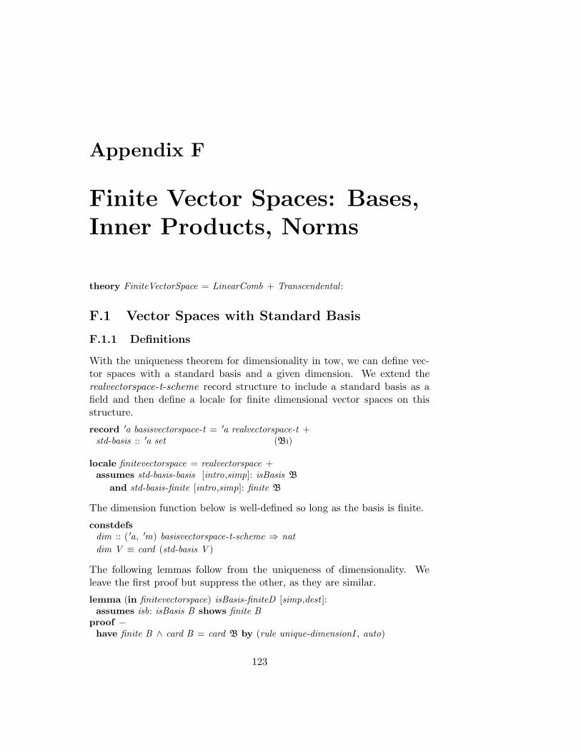
Appendix F
Finite Vector Spaces: Bases,Inner Products, Norms
theory FiniteVectorSpace = LinearComb + Transcendental :
F.1 Vector Spaces with Standard Basis
F.1.1 Definitions
With the uniqueness theorem for dimensionality in tow, we can define vec-tor spaces with a standard basis and a given dimension. We extend therealvectorspace-t-scheme record structure to include a standard basis as afield and then define a locale for finite dimensional vector spaces on thisstructure.
record ′a basisvectorspace-t = ′a realvectorspace-t +std-basis :: ′a set (Bı)
locale finitevectorspace = realvectorspace +assumes std-basis-basis [intro,simp]: isBasis B
and std-basis-finite [intro,simp]: finite B
The dimension function below is well-defined so long as the basis is finite.
constdefsdim :: ( ′a, ′m) basisvectorspace-t-scheme ⇒ nat
dim V ≡ card (std-basis V )
The following lemmas follow from the uniqueness of dimensionality. Weleave the first proof but suppress the other, as they are similar.
lemma (in finitevectorspace) isBasis-finiteD [simp,dest ]:assumes isb: isBasis B shows finite B
proof −have finite B ∧ card B = card B by (rule unique-dimensionI , auto)
123

124APPENDIX F. FINITE VECTOR SPACES: BASES, INNER PRODUCTS, NORMS
thus finite B ..qed
lemma (in finitevectorspace) isBasis-cardD [simp,dest ]:assumes isBasis B shows card B = dim V
lemma (in finitevectorspace) isBasis-baseD [simp,dest ]: isBasis B =⇒ base Bby (rule, auto)
F.1.2 Decomposition over a Finite Basis
Given a finite dimensional vector space and any basis, there is a unique co-efficient function that represents any given vector v. We define an operationdecompose that produces this coefficient function. Since it is an ’inverse’ tothe linear combination operation, we give it a syntax of v B.
This definition takes us head-long into the issue of partiality – in order touse THE to define the decomposition, we have to make a choice for theparticular extension of the coefficent function to the UNIV of vectors. Asa matter of principle, we have not used any definitions of convenience forwhat should be undefined values and we shall accordingly use the set ofextensional functions to make this selection ‘arbitrary’.
constdefsdecompose :: ( ′a, ′m) realvectorspace-t-scheme ⇒ ′a ⇒ ′a set ⇒ ( ′a ⇒ real)
(infix ı 150 )decompose V v B ≡ THE a. (lc-prod V a B = v) ∧ a ∈ extensional B
— Show existence of basis decomposition.lemma (in finitevectorspace) basis-decomp-ex : [[ isBasis B ; v ∈ carrier V ]] =⇒∃ a. a · B = vby (rule base-mem-spanD ,auto)
— Show uniqueness
The uniqueness of decomposition over a basis B follows from the linearindependence of B. We thus prove the following slightly more general result.
theorem (in finitevectorspace) linearind-decomp-uniq :assumes linindB : linearind B and baseB : base B
and vals : a · B = v b · B = vshows ∀ e∈B . a e = b e
prooffix e assume einB : e ∈ B
show a e = b eproof (rule ccontr)assume a e 6= b ewith einB have nontrivial (λv . a v − b v) B by auto
moreover have (λv . a v − b v) · B = 0 proof −

F.1. VECTOR SPACES WITH STANDARD BASIS 125
have (λv . a v − b v) · B = a · B b · B by (simp! add : lc-prod-lm-distrib)also have . . . = v v using vals by (simp)also have . . . = 0 by (simp! add : vals [symmetric])finally show ?thesis .
qed
ultimately have lineardep B using baseB by auto
with linindB show False by contradictionqed
qed
lemma (in finitevectorspace) basis-decomp-uniq :assumes basisB : isBasis B
and vals : a · B = v b · B = vshows ∀ e∈B . a e = b eby (intro linearind-decomp-uniq , auto!)
lemmas (in finitevectorspace) basis-decomp-uniqD = basis-decomp-uniq [rule-format ]
— The simp rule that we get when the decomposition is well defined.
lemma (in finitevectorspace) basis-decomp-well-def [simp]:assumes basisB : isBasis B and vincar : v ∈ carrier V shows v B · B = v
proof −have ∃ a. a · B = v by (rule basis-decomp-ex )then obtain a where a · B = v by blastdef a ′ ≡ restrict a Bhave a ′val : a ′ · B = v using basisB by (simp add : a ′-def )have a ′ext : a ′ ∈ extensional B by (auto simp: a ′-def )
show (v B) · B = vproof (unfold decompose-def , rule theI2 [of λa. a · B = v ∧ a ∈ extensional
B ])from a ′val a ′ext show a ′ · B = v ∧ a ′ ∈ extensional B by (auto)
fix x assume x · B = v ∧ x ∈ extensional Bhence xval : x · B = v and xext : x ∈ extensional B by blast+
from xext a ′ext show x = a ′
proof (rule extensionalityI )fix v assume v ∈ Bfrom basisB xval a ′val show x v = a ′ v by (rule basis-decomp-uniqD)
qedqed (auto)
qed
lemma (in finitevectorspace) basis-decomp-equal :assumes asm: isBasis B v ∈ carrier V w ∈ carrier V

126APPENDIX F. FINITE VECTOR SPACES: BASES, INNER PRODUCTS, NORMS
and compeq : ∀ e ∈ B . (v B) e = (w B) eshows v = w
proof −from asm have v = v B · B by simpalso from asm compeq have . . . = w by simpfinally show ?thesis .
qed
Calculational Properties of Decomposition
lemma (in finitevectorspace) basis-decomp-zero:assumes basisB : isBasis Bshows ∀ e∈B . (0 B) e = 0by (auto! intro: basis-decomp-uniqD)
lemmas (in finitevectorspace) basis-decomp-zeroD [simp] = basis-decomp-zero [rule-format ]
lemma (in finitevectorspace) basis-decomp-distrib:assumes isBasis B and a ∈ carrier V b ∈ carrier Vshows ∀ e∈B . ((a ⊕ b) B) e = (a B) e + (b B) e
prooffix e assume e ∈ Bshow ((a ⊕ b) B) e = (a B) e + (b B) eproof (rule basis-decomp-uniqD)show (a ⊕ b) B · B = a ⊕ b by (simp!)show (λu. (a B) u + (b B) u) · B = a ⊕ b by (simp! add : lc-prod-l-distrib)
qed (auto!)qed
lemmas (in finitevectorspace) basis-decomp-distribD [simp] = basis-decomp-distrib[rule-format ]
lemma (in finitevectorspace) basis-decomp-factor :assumes isBasis B and a ∈ carrier Vshows ∀ e∈B . ((r · a) B) e = r ∗ (a B) e
prooffix e assume e ∈ Bshow ((r · a) B) e = r ∗ (a B) eproof (rule basis-decomp-uniqD)show (r · a) B · B = r · a by (simp!)show (λu. r ∗ (a B) u) · B = r · a by (simp! add : lc-prod-factor)
qed (auto!)qed
lemmas (in finitevectorspace) basis-decomp-factorD [simp] = basis-decomp-factor [rule-format ]

F.2. STANDARD INNER PRODUCT 127
F.2 Standard Inner Product
F.2.1 Definition
We define the standard inner product on a finite vector space with basis.And show that it has the definitive properties of a general inner product.Namely,
• Bilinearity
• Symmetry
• Positive definiteness
constdefsstd-iprod :: ( ′a, ′m) basisvectorspace-t-scheme ⇒ ′a ⇒ ′a ⇒ real (〈-,-〉ı 1000 )std-iprod V a b ≡ (
∑e:std-basis V . (decompose V a (std-basis V )) e ∗ (decompose
V b (std-basis V )) e)
F.2.2 Properties
lemma (in finitevectorspace) iprod-commute [simp]:assumes a ∈ carrier V b ∈ carrier Vshows 〈a, b〉 = 〈b, a〉
by (simp add : std-iprod-def ring-eq-simps)
lemma (in finitevectorspace) iprod-linear1 [simp]:assumes a ∈ carrier V b ∈ carrier V c ∈ carrier Vshows 〈a ⊕ b, c〉 = 〈a,c〉 + 〈b,c〉
by (simp! add : std-iprod-def ring-eq-simps setsum-addf cong : setsum-cong)
lemma (in finitevectorspace) iprod-linear2 [simp]:assumes a ∈ carrier V b ∈ carrier V c ∈ carrier Vshows 〈a, b ⊕ c〉 = 〈a,b〉 + 〈a,c〉
by (simp! add : std-iprod-def ring-eq-simps setsum-addf cong : setsum-cong)
lemma (in finitevectorspace) iprod-scale1 [simp]:assumes a ∈ carrier V b ∈ carrier Vshows 〈r · a, b〉 = r ∗ 〈a, b〉
by (simp! add : std-iprod-def setsum-l-factor ring-eq-simps cong : setsum-cong)
lemma (in finitevectorspace) iprod-scale1 [simp]:assumes a ∈ carrier V b ∈ carrier Vshows 〈a, r · b〉 = r ∗ 〈a, b〉
by (simp! add : std-iprod-def setsum-l-factor ring-eq-simps cong : setsum-cong)
lemma (in finitevectorspace) iprod-nonneg :assumes a ∈ carrier Vshows 0 ≤ 〈a, a〉
by (unfold std-iprod-def , auto intro: setsum-nonneg)

128APPENDIX F. FINITE VECTOR SPACES: BASES, INNER PRODUCTS, NORMS
lemma (in finitevectorspace) iprod-zerodef :assumes a ∈ carrier V and zero: 〈a, a〉 = 0shows a = 0
proof (rule basis-decomp-equal [of B], simp-all !)show ∀ e∈B. (a B) e = 0proof (rule, rule ccontr)let ?aB = a B
fix e assume einB : e ∈ B and nz : ?aB e 6= 0
have 〈a, a〉 = (∑
f :B. ?aB f ∗ ?aB f ) by (simpadd : std-iprod-def )
also from std-basis-finite einB have . . . = ?aB e ∗ ?aB e + (∑
f :B − e.?aB f ∗ ?aB f )
by (simp add :setsum-diff1-gen)
finally have eqn: 0 = ?aB e ∗ ?aB e + (∑
f :B − e. ?aB f ∗ ?aB f ) usingzero by simp
have 0 ≤ ?aB e ∗ ?aB e by simpwith nz have pos : 0 < ?aB e ∗ ?aB e by (simp add : order-le-less)
have nonneg : 0 ≤ (∑
f :B − e. ?aB f ∗ ?aB f ) by (auto intro: setsum-nonneg)
from eqn pos nonneg have 0 < 0 by ariththus False ..
qedqed
lemma (in finitevectorspace) iprod-zerodef-cont :a ∈ carrier V =⇒ a 6= 0 =⇒ 〈a,a〉 6= 0
by (insert iprod-zerodef , blast)
lemma (in finitevectorspace) iprod-lzero-zero:assumes [simp]: a ∈ carrier Vshows 〈0,a〉 = 0
by (simp add : std-iprod-def setsum-0 cong : setsum-cong)
lemma (in finitevectorspace) iprod-rzero-zero:assumes [simp]: a ∈ carrier Vshows 〈a,0〉 = 0
by (simp add : std-iprod-def setsum-0 cong : setsum-cong)
lemmas (in finitevectorspace) iprod-zero-zero [simp] = iprod-lzero-zero iprod-rzero-zero

F.3. STANDARD NORM 129
F.3 Standard Norm
F.3.1 Definition
We define the norm in the normal way from the standard inner product andthen show that it has all the properties of a norm:
• Positive definiteness
• The Schwartz Inequality
• The Triangle Inequality
• Linear Scaling
constdefsstd-norm :: ( ′a, ′m) basisvectorspace-t-scheme ⇒ ′a ⇒ real (‖-‖ı 1000 )std-norm V a ≡ sqrt (std-iprod V a a)
F.3.2 Basic Properties
lemma (in finitevectorspace) norm-nonneg :assumes a ∈ carrier Vshows 0 ≤ ‖a‖
proof (unfold std-norm-def )have 0 ≤ 〈a,a〉 by (rule iprod-nonneg)hence sqrt 0 ≤ sqrt 〈a,a〉 by (intro real-sqrt-le-mono, arith+)thus 0 ≤ sqrt 〈a,a〉 by simp
qed
lemma (in finitevectorspace) norm-power2-iprod :assumes [simp]: a ∈ carrier Vshows ‖a‖2 = 〈a,a〉
by (simp add : std-norm-def iprod-nonneg)
lemma (in finitevectorspace) norm-zerodef :assumes [simp]: a ∈ carrier V and zero: ‖a‖ = 0shows a = 0
proof −have 〈a,a〉 = ‖a‖2 by (simp add : norm-power2-iprod)also have . . . = 0 using zero by simpfinally show a = 0 by (auto! intro: iprod-zerodef )
qed
lemma (in finitevectorspace) norm-zerodef-cont :a ∈ carrier V =⇒ a 6= 0 =⇒ ‖a‖ 6= 0
by (insert norm-zerodef , blast)
lemma (in finitevectorspace) norm-scale [simp]:

130APPENDIX F. FINITE VECTOR SPACES: BASES, INNER PRODUCTS, NORMS
assumes [simp]: a ∈ carrier Vshows ‖r · a‖ = |r | ∗ ‖a‖
proof −have ‖r · a‖ = sqrt 〈r · a, r · a〉 by (simp add : std-norm-def )also have . . . = sqrt (r ∗ r ∗ 〈a,a〉) by (simp add : ring-eq-simps)also have . . . = sqrt (r ∗ r) ∗ sqrt 〈a,a〉using iprod-nonneg by (simp add : real-sqrt-mult-distrib2 )
also have . . . = |r | ∗ ‖a‖ by (simp add : std-norm-def )finally show ?thesis .
qed
lemma (in finitevectorspace) norm-zero-zero[simp]: ‖0‖ = 0proof −have ‖0‖ = ‖0 · 0‖ by simpalso have . . . = |0 | ∗ ‖0‖ by (simp only : norm-scale zero-closed)also have . . . = 0 by simpfinally show ?thesis .
qed
lemma (in finitevectorspace) norm-schwartz-equal :assumes [simp]: a ∈ carrier V
and val : b = r · ashows |〈a,b〉| = ‖a‖ ∗ ‖b‖
proof −from val have |〈a,b〉| = |r | ∗ |〈a,a〉| by simpalso have . . . = |r | ∗ ‖a‖ ∗ ‖a‖using iprod-nonneg norm-nonnegby (simp add : std-norm-def real-sqrt-pow-abs power2-eq-square[symmetric])
also have . . . = ‖a‖ ∗ ‖r · a‖ by (simp add : norm-scale)also have . . . = ‖a‖ ∗ ‖b‖ using val by simpfinally show ?thesis .
qed
lemma (in finitevectorspace) norm-schwartz :assumes [simp]: a ∈ carrier V b ∈ carrier Vshows |〈a,b〉| ≤ ‖a‖ ∗ ‖b‖
proof (cases 0 ∈ a, b)assume notzero: 0 /∈ a, bshow ?thesisproof (cases lineardep a,b)assume ld : lineardep a,bhave diff : a 6= b proofassume aneb: a = bwith notzero have linearind a by (intro singleton-linearindI , auto)moreover from aneb ld have lineardep a by simpultimately show False by contradiction
qed

F.3. STANDARD NORM 131
have finite a,b by autowith ld obtain vc v where vin: v ∈ a,b and vcval : vc · (a,b − v) = v
using finite-lineardep-solve by (blast)
— lineardependence implies equality hereshow |〈a,b〉| ≤ ‖a‖ ∗ ‖b‖proof (cases v = a)assume visa: v = ahence a = v by simpalso from vcval have . . . = vc · (a,b − v) by simpalso from visa diff have . . . = vc b · b by (simp add : lc-prod-value)finally have aval : a = vc b · b .
hence |〈b,a〉| = ‖b‖ ∗ ‖a‖ by (intro norm-schwartz-equal)hence |〈a,b〉| = ‖a‖ ∗ ‖b‖ by simpthus ?thesis by arith
nextassume v 6= awith vin have visb: v = b by blasthave abba: a, b = b, a by blast
from visb have b = v by simpalso from vcval abba have . . . = vc · (b,a − v) by simp
also from visb diff [symmetric] have . . . = vc a · a by (simp add : lc-prod-value)finally have bval : b = vc a · a .
hence |〈a,b〉| = ‖a‖ ∗ ‖b‖ by (intro norm-schwartz-equal)thus ?thesis by arith
qed
nextassume linearind a,b
show ?thesis proof (cases a = b)assume a = bhence b = 1 · a by simphence |〈a,b〉| = ‖a‖ ∗ ‖b‖ by (intro norm-schwartz-equal)thus ?thesis by arith
nextassume aneb: a 6= b
fix rhave incar [simp]: −1 · a ⊕ r · b ∈ carrier V by auto
have noeigen: −1 · a ⊕ r · b 6= 0 proofassume lc: −1 · a ⊕ r ·b = 0

132APPENDIX F. FINITE VECTOR SPACES: BASES, INNER PRODUCTS, NORMS
have lineardep a,b proof (intro lineardepI )let ?c = λv . if v = b then r else −1from lc aneb show ?c · a,b = 0 by (simp add : lc-prod-value Pi-def )
from aneb show nontrivial ?c a,b by (intro nontrivialI , auto)qed (auto)
moreover have linearind a, b .ultimately show False by contradiction
qed
have ‖−1 · a ⊕ r · b‖ 6= 0 proofassume ‖−1 · a ⊕ r · b‖ = 0hence −1 · a ⊕ r · b = 0 by (auto intro!: norm-zerodef )with noeigen show False by contradiction
qed
moreover have 0 ≤ ‖−1 · a ⊕ r · b‖ by (auto intro: norm-nonneg)ultimately have 0 < ‖−1 · a ⊕ r · b‖ by arith
hence 0 < ‖−1 · a ⊕ r · b‖2 by simpalso have . . . = 〈−1 · a ⊕ r · b,−1 · a ⊕ r · b〉using iprod-nonneg [OF incar ] by (simp add : abs-if std-norm-def real-sqrt-pow-abs)also have . . . = r ∗ r ∗ 〈b,b〉 + −2 ∗ r ∗ 〈a,b〉 + 〈a,a〉 by simpfinally have 0 < 〈b,b〉 ∗ r2 + (−2 ∗ 〈a,b〉) ∗ r + 〈a,a〉 by (simp add :
ring-eq-simps power2-eq-square)note no-quadratic-roots = this
have (−2 ∗ 〈a,b〉)2 − 4 ∗ 〈b,b〉 ∗ 〈a,a〉 < 0 (is ?disc < 0 )proof (rule ccontr , simp only : linorder-not-less)assume posdisc: 0 ≤ ?discfrom notzero have b 6= 0 by blasthence 〈b,b〉 6= 0 by (simp add : iprod-zerodef-cont)with posdisc obtain r where soln: 〈b,b〉 ∗ r 2 + (−2 ∗ 〈a,b〉) ∗ r + 〈a,a〉
= 0using quadratic-formula by blast
from no-quadratic-roots have 0 < 〈b,b〉 ∗ r 2 + (−2 ∗ 〈a,b〉) ∗ r + 〈a,a〉 .hence 〈b,b〉 ∗ r2 + (−2 ∗ 〈a,b〉) ∗ r + 〈a,a〉 6= 0 by simpwith soln show False by contradiction
qed
hence 4 ∗ 〈a,b〉2 < 4 ∗ 〈a,a〉 ∗ 〈b,b〉 by (simp add : power2-eq-squarering-eq-simps)
hence 〈a,b〉2 < 〈a,a〉 ∗ 〈b,b〉 by (simp)with - have sqrt (〈a,b〉2) < sqrt(〈a,a〉 ∗ 〈b,b〉) by (rule real-sqrt-less-mono,
auto)

F.3. STANDARD NORM 133
hence |〈a,b〉| < sqrt(〈a,a〉) ∗ sqrt(〈b,b〉)using iprod-nonneg by (simp add : real-sqrt-mult-distrib2 )
hence |〈a,b〉| < ‖a‖ ∗ ‖b‖ by (simp add : std-norm-def )thus ?thesis by simp
qedqed
nextassume haszero: 0 ∈ a,bthus ?thesis proof (cases a = 0)assume azero: a = 0thus |〈a,b〉| ≤ ‖a‖ ∗ ‖b‖ by simp
nextassume a 6= 0with haszero have b = 0 by blastthus ?thesis by simp
qedqed
lemma (in finitevectorspace) norm-triangle:assumes [simp]: a ∈ carrier V b ∈ carrier Vshows ‖a ⊕ b‖ ≤ ‖a‖ + ‖b‖
proof −have ‖a ⊕ b‖2 = 〈a,a〉 + 〈b,b〉 + 2 ∗ 〈a,b〉 by (simp add : norm-power2-iprod)also have . . . ≤ |〈a,a〉 + 〈b,b〉 + 2 ∗ 〈a,b〉| by (simp only : abs-ge-self )also have . . . ≤ |〈a,a〉| + |〈b,b〉| + 2 ∗ |〈a,b〉| by arithalso have . . . = |‖a‖2| + |‖b‖2| + 2 ∗ |〈a,b〉| by (simp add : norm-power2-iprod
)also have . . . ≤ ‖a‖2 + ‖b‖2 + 2 ∗ ‖a‖∗‖b‖ using norm-schwartz by
simpalso have . . . = (‖a‖ + ‖b‖)2 by (simp add : power2-eq-square
ring-eq-simps)finally have ‖a ⊕ b‖2 ≤ (‖a‖ + ‖b‖)2 .
hence sqrt (‖a ⊕ b‖2) ≤ sqrt ((‖a‖ + ‖b‖)2) by (intro real-sqrt-le-mono,auto)moreover from norm-nonneg have 0 ≤ ‖a ⊕ b‖ 0 ≤ ‖a‖ 0 ≤ ‖b‖ by automoreover hence 0 ≤ ‖a‖ + ‖b‖ by arithultimately show ‖a ⊕ b‖ ≤ ‖a‖ + ‖b‖ by (simp add : power2-eq-square, arith)
qed
end