AN HYBRID APPROACH TO SOLVE TRAVELING

SALESMAN PROBLEM USING GENETIC ALGORITHM

CENGIZ ASMAZOGLU

B.S., Computer Engineering, Isık University, 2010

Submitted to the Graduate School of Science and Engineering

in partial fulfillment of the requirements for the degree of

Master of Science

in

Computer Engineering

ISIK UNIVERSITY

2013

ISIK UNIVERSITY

GRADUATE SCHOOL OF SCIENCE AND ENGINEERING

AN HYBRID APPROACH TO SOLVE TRAVELING SALESMAN PROBLEM

USING GENETIC ALGORITHM

CENGIZ ASMAZOGLU

APPROVED BY:

Assoc. Prof. Olcay Taner Yıldız Isık University

(Thesis Supervisor)

Assist. Prof. Ali Inan Isık University

Assist. Prof. Osman Murat Anlı Isık University

APPROVAL DATE: ..../..../....

A DYNAMIC APPROACH FOR TRAVELING

SALESMAN PROBLEM USING GENETIC

ALGORITHMS

Abstract

TSP is a challenging and popular problem from combinatorial optimization. TSP

is often tackled with well known heuristic genetic algorithm. Due to the nature

of the TSP, traditional GA’s stay poor when competing with other approaches.

Traditional crossover and mutation operators do not satisfy TSP needs. These

operators mostly end up with illegal tours. For this reason, researchers proposed

many adaptive elements and cooperation of other algorithms. When the logic

of GA is combined with these elements, high quality solutions both in time and

path length are obtained.

In this research, we analyze successful elements from the literature to use them

efficiently in a novel algorithm. We also propose a new selection method which

works well with our operators. We extend the abilities of greedy crossover and

untwist local operator to utilize in our hybrid approach. Multiple populations

collaborate together to achieve better solutions. According to the experimen-

tal results, proposed novel elements outperforms their counterparts in the TSP

literature. Multiple population approach provides better quality solutions.

ii

GEZEN POSTACI PROBLEMINE GENETIK

ALGORITMA KULLANARAK DINAMIK YAKLASIM

Ozet

Gezgin postacı problemi, kombinasyonel optimizasyon sınıfından zorlu ve populer

bir problemdir. Bu problem sıklıkla genetik algoritma ile cozumlenir. Bu prob-

lemin dogası geregi, geleneksel genetik algoritmalar baska yaklasımlar ile karsılastırıldıgında

zayıf kalır. Geleneksel ciftlesme ve mutasyon yontemleri bu problemin cozumu

icin yetersiz kalmaktadır. Bu operatorlerin kullanımı cogunlukla uygun olmayan

turlarla sonlanır. Bu sebepten dolayı, arastırmacılar bu probleme uygun olarak

genetik algoritma ile kombine calısacak elemanlar onermisler ve sonucunda tur

kalitesi ve zaman acısından kaliteli cozumler cıkarmıslardır.

Bu arastırmada, literaturden basarılı elemanları analiz edip kendi onerdigimiz al-

goritmamızda efektif olarak kullanmak istedik. Ayrıca, bizim operatorlerimizle iyi

calısan yeni bir secim yontemi onerdik. Bizim hibrid yaklasımımızda kullanmak

uzere, greedy ciftlesme ve untwist yerel operatorlerinin yetkinliklerini genislettik.

Coklu populasyonlar birlikte calısarak daha iyi sonuclar vermektedir. Deneysel

sonuclarımıza gore, onerdigimiz yeni elemanlar literaturdeki muadillerini geride

bırakmaktadır.

iii

Acknowledgements

There are many people who helped me make my years at the graduate school

most valuable. First, I would like to express my deepest acknowledgements to

my supervisor Assoc. Prof. Olcay Taner Yıldız for his support and guidance

throughout my thesis work. I am also thankful to Isık University for providing

me all the facilities and for being a part of such a wonderful environment. Finally,

I will always be indebted to my wife Duygu and my mother Cevriye for their

patience and encouragement.

iv

To my family. . .

Table of Contents

Abstract ii

Ozet iii

Acknowledgements iv

List of Figures viii

List of Tables ix

List of Abbreviations x

1 Introduction 1

2 Literature Review 4

2.1 Representations . . . . . . . . . . . . . . . . . . . . . . . . . . . . 5

2.2 Selection . . . . . . . . . . . . . . . . . . . . . . . . . . . . . . . . 6

2.3 Crossover . . . . . . . . . . . . . . . . . . . . . . . . . . . . . . . 7

2.3.1 Partially Mapped Crossover . . . . . . . . . . . . . . . . . 8

2.3.2 Cycle Crossover . . . . . . . . . . . . . . . . . . . . . . . . 9

2.3.3 Order Crossover . . . . . . . . . . . . . . . . . . . . . . . . 10

2.3.4 Distance Preserving Crossover . . . . . . . . . . . . . . . . 10

2.3.5 Alternating Positions Crossover . . . . . . . . . . . . . . . 11

2.3.6 Greedy Crossover . . . . . . . . . . . . . . . . . . . . . . . 12

2.3.7 Complete Subtour Exchange . . . . . . . . . . . . . . . . . 13

2.3.8 Sorted Match Crossover . . . . . . . . . . . . . . . . . . . 14

2.4 Mutation . . . . . . . . . . . . . . . . . . . . . . . . . . . . . . . . 15

2.4.1 Reciprocal Exchange Mutation . . . . . . . . . . . . . . . 16

2.4.2 Insertion Mutation . . . . . . . . . . . . . . . . . . . . . . 16

2.4.3 Displacement Mutation . . . . . . . . . . . . . . . . . . . . 17

2.4.4 Simple Inversion Mutation . . . . . . . . . . . . . . . . . . 18

2.4.5 Inversion Mutation . . . . . . . . . . . . . . . . . . . . . . 18

2.4.6 Scramble Mutation . . . . . . . . . . . . . . . . . . . . . . 19

2.4.7 Ends Exchange Mutation . . . . . . . . . . . . . . . . . . . 19

2.4.8 Reverse Ends Mutation . . . . . . . . . . . . . . . . . . . . 20

2.4.9 Reverse Ends Exchange Mutation . . . . . . . . . . . . . . 20

2.5 Local Operators . . . . . . . . . . . . . . . . . . . . . . . . . . . . 21

2.5.1 2-opt . . . . . . . . . . . . . . . . . . . . . . . . . . . . . . 21

2.5.2 3-opt . . . . . . . . . . . . . . . . . . . . . . . . . . . . . . 22

2.5.3 Lin-Kernighan Opt . . . . . . . . . . . . . . . . . . . . . . 23

2.5.4 Remove Sharp . . . . . . . . . . . . . . . . . . . . . . . . . 24

2.5.5 LocalOpt . . . . . . . . . . . . . . . . . . . . . . . . . . . 24

2.5.6 Untwist . . . . . . . . . . . . . . . . . . . . . . . . . . . . 25

3 Proposed Algorithm 26

3.1 Greedy k-nn Crossover . . . . . . . . . . . . . . . . . . . . . . . . 26

3.2 Greedy Selection . . . . . . . . . . . . . . . . . . . . . . . . . . . 30

3.3 Extended Untwist . . . . . . . . . . . . . . . . . . . . . . . . . . . 30

3.4 Other Elements . . . . . . . . . . . . . . . . . . . . . . . . . . . . 31

3.5 The Algorithm . . . . . . . . . . . . . . . . . . . . . . . . . . . . 31

4 Experiments 33

4.1 Experimental Setup . . . . . . . . . . . . . . . . . . . . . . . . . . 33

4.2 Experimental Results . . . . . . . . . . . . . . . . . . . . . . . . . 33

5 Conclusion 36

References 38

Curriculum Vitae 40

List of Figures

1.1 A visualization of symmetric TSP. (a) a twisted bad route (b) theoptimum route . . . . . . . . . . . . . . . . . . . . . . . . . . . . 1

2.1 Hybrid GA Model . . . . . . . . . . . . . . . . . . . . . . . . . . . 4

viii

List of Tables

2.1 Well-known crossover operators in the literature . . . . . . . . . . 7

2.2 Well-known mutation operators in the literature . . . . . . . . . . 16

2.3 Well-known local operators in the literature . . . . . . . . . . . . 21

3.1 The number of k-nearest neighbours appearing in the optimal tour 26

3.2 Distance Matrix D . . . . . . . . . . . . . . . . . . . . . . . . . . 28

4.1 Algorithm Parameters . . . . . . . . . . . . . . . . . . . . . . . . 33

4.2 Experimental Results . . . . . . . . . . . . . . . . . . . . . . . . . 34

4.3 Experimental Results with one population . . . . . . . . . . . . . 34

4.4 Experimental Results with PMX . . . . . . . . . . . . . . . . . . 34

4.5 Experimental Results with k = 1 . . . . . . . . . . . . . . . . . . 35

4.6 Experimental Results with TS . . . . . . . . . . . . . . . . . . . . 35

ix

List of Abbreviations

TSP Traveling Salesman Problem

GA Genetic Algorithm

N Total Number of Cities

D Distance Function

C A City

(1, 2, 3, 4, 5, 6) A Complete Tour

[3, 4, 5] A Subtour

{(), [], 1, 2, 3} A Group of Subtour(s) and/or Tour(s) and/or City(ies)

k-nn k-Nearest Neighbor

PMX Partially Mapped Crossover

CX Cycle Crossover

OX Order Crossover

DPX Distance Preserving Crossover

APX Alternating Positions Crossover

GX Greedy Crossover

CSEX Complete Subtour Exchange Crossover

SMX Sorted Match Crossover

REM Reciprocal Exchange Mutation

IM Insertion Mutation

DM Displacement Mutation

SIM Simple Inversion Mutation

IVM Inversion Mutation

SM Scramble Mutation

ESEM Ends Exchange Mutation

x

RESM Reverse Ends Mutation

RESEM Reverse Ends Exchange Mutation

RWS Roulette Wheel Selection

TS Tournament Selection

xi

Chapter 1

Introduction

TSP, is one of the most important problems in combinatorial optimization. It was

first formulated by the mathematician Karl Menger in 1930 and belongs to the

set of NP-Hard problems. Given a list of N cities, a salesman tries to visit all of

the cities only once, where he/she minimizes the path length. The running time

of the problem grows exponentially with respect to the number of cities, i.e. the

number of possible solutions is N!. To overcome the issue, lots of research have

been presented but no one is able to state an algorithm that finds the optimal

route in polynomial time.

Figure 1.1: A visualization of symmetric TSP. (a) a twisted bad route (b) theoptimum route

Considerable number of variations exists for the TSP. Some of these are; asym-

metric TSP, multiple TSP, clustered TSP etc. In symmetric TSP (STSP) each

city pair have the same distance for both directions. We represent an example of

STSP in Figure 1.1. Figure 1.1 (a) and (b) show a non-optimal solution and the

1

optimal solution to the example STSP respectively. Asymmetric TSP is similar to

the symmetric TSP where the distance between two cities is not equal or no path

exists for one direction. In multiple TSP, salesmen collaborate to achieve a target

solution. In clustered TSP, there are clusters composed of adjacent cities. These

clusters behave as a single city to decrease the number of cities and therefore

improve running time. We focus on STSP in this thesis.

In history, two types of algorithms are designed for this challenge; exact algo-

rithms and heuristic algorithms. Exact algorithms apply brute force search tech-

niques and try to minimize the search space with specific constraints. They may

find the optimal tour but the time complexity is not satisfactory especially when

the number of cities is large, i.e. N > 1000. Linear programming is an example

of exact algorithms. Concorde TSP Solver is arguably the best program [1] to

solve TSP using linear programming concepts.

Heuristic algorithms traverse the search space randomly and try to approach the

global optimum. For these approaches, we are less likely to reach the global opti-

mum as exact algorithms do. On the other hand, time complexities of the heuristic

algorithms are far better than the exact algorithms. Ant colony optimization and

simulated annealing algorithms are well-known examples of heuristic approaches.

They can compete with genetic algorithms and can also perform as internal GA

elements.

GA’s are one of the optimization algorithms. A typical GA has several steps. We

first initialize an individual (chromosome) array, i.e. population. Then we iterate

on this population until a satisfactory solution is found. The unit of iteration is

known as a generation, and an iteration consists of applying operators consistent

with the nature of the GA. The basic operators are crossover and mutation.

Crossover operator exchanges information between two individuals known as par-

ents. We select the parents with a selection method and form offspring(s) from

the chromosomes of parents. The selection method is based on a fitness value

which indicates the wellness of an individual.

2

Mutation operator is often executed on a single individual. It is inspired by

the nature to diverse the chromosomes of the population. This operator tries to

prevent the algorithm from getting stuck at local optima. At each generation,

operators try to improve the population to reach a near-optimal solution.

In TSP, GA’s are suffering from stucking at local optima because of the ordering

issues in the routing structure. So, using a pure GA for TSP is not a strong idea.

Classical crossover operators are not suitable for TSP. In the literature, many

authors have proposed useful crossover designs to meet TSP features. Some

handy mutation operators are also proposed in the literature to solve TSP with

GA. Other elements that works well with GA on TSP are local operators, hybrid

approaches, artificial chromosome generator, etc. The designer should be aware

of effective cooperation between crossover, mutation, and local operators.

In this thesis, we try to solve STSP with a specialized GA approach. We pro-

pose greedy k-nn crossover as the crossover model and a new selection method

named greedy selection. We compare these novel elements with their counter-

parts from the TSP literature. In addition, we analyze how multiple populations

improve solution quality with smart immigration. According to experimental re-

sults, multiple population design outperforms single population in terms of tour

quality.

This thesis is organized as follows: We give the literature review on GA’s in

Chapter 2. We explain our proposed approach in detail in Chapter 3. We give

experimental results in Chapter 4 and conclude in Chapter 5.

3

Chapter 2

Literature Review

There is no wonder why TSP is so challenging. Being in the problem set of

NP-Hard and its simple formulation, so many people are fascinated to propose

a solution. Due to its exponential running time, researchers tend to solve this

problem via heuristic approaches rather than exact algorithms. According to its

simple structure and tweakable form, GA’s can stand as a role model for all other

heuristic optimizations in TSP. For this reason, many authors have proposed an

hybrid structure of GA to solve TSP. We present this hybrid model in Figure 2.1.

We first initialize the population. According to the parameters of the approach,

we apply selected elements to get a new population. If the best individual of

the new population satisfies a pregiven criteria, we stop and return to the best

solution. Otherwise, we continue iteration by applying selected elements to the

new population.

Figure 2.1: Hybrid GA Model

4

Section 2.1 explains different representations of a chromosome. Section 2.2 de-

scribes selection methods. Sections 2.3 and 2.4 cover fundamental genetic opera-

tors crossover and mutation for TSP respectively. Local operators are described

in Section 2.5.

2.1 Representations

In the literature, researchers have proposed several alternatives to represent chro-

mosomes in GA for TSP. Well known representations are binary representation,

path representation, adjacency representation, ordinal representation, and matrix

representation.

In binary representation, we encode N cities using dlog2Ne bits. The tour given

in Figure 1.1 (a) is represented as:

( 000︸︷︷︸0

100︸︷︷︸4

101︸︷︷︸5

010︸︷︷︸2

111︸︷︷︸7

011︸︷︷︸3

001︸︷︷︸1

110︸︷︷︸6

)

Path representation is the most used representation. We basicly represent the

tour in the Figure 1.1 (b) as follows:

(1, 2, 3, 4, 5, 6, 7, 8)

Path representation is a base representation to solve TSP using GA analogy. We

assume that all paths should be cyclic to provide a complete tour. Our proposed

algorithm uses path representation.

There exist also other representations; such as adjacency, ordinal and matrix rep-

resentations. But, these representations are not used anymore for GA approaches.

5

2.2 Selection

Selection is very critical in GA because the process will be completely random

without it. The element is inspired by the natural selection phenomenon of the

evolution. Crossover designs work better with specific selection methods to im-

prove the population quality. Such selection methods are; roulette wheel selection

(RWS) and tournament selection (TS).

RWS algorithm 2.2 is based on the idea that, the individual’s selection probability

is proportional with its fitness score like in the natural selection. In RWS, all

individuals are sorted according to their fitness scores (Lines 1-2). We calculate

an array of sum of fitnesses for the population (Line 3). sumOfFitnesses[i]

stores the sum of fitnesses of all individuals indexes through 0 to i. Then, we

generate a random value between 0 and last element of the array which is sum

of all fitnesses of the population (Line 4). To select an index, we iterate through

the array and look for the first index where the random value is larger than the

sum of fitnesses until that index (Lines 5-9).

Algorithm 1 Roulette Wheel Selection

1: population.evaluateFitnesses()2: population.sortIndividuals()3: sumOfFitnesses = population.generateSumOfFitnesses()4: value = random(0, sumOfFitnesses[lastElement])5: for i = 0 to sumOfFitnesses.length do6: if value < sumOfFitnesses[i] then7: return i8: end if9: end for

In TS algorithm 2, we first evaluate and sort all the chromosomes in a population

(Lines 1-2). Then, we simply generate a random number to pick that amount

of individuals from the population (Lines 3-4). Then we select the fittest among

them (Lines 5-11). Setting aNumber as 1 will result in 100% random selection.

6

Algorithm 2 Tournament Selection

1: population.evaluateFitnesses()2: population.sortIndividuals()3: shortest = ∞4: aNumber = random(0, N)5: for i = 0 to aNumber do6: index = random(0, N)7: if length(tour[index]) < shortest then8: shortest = length(tour[index])9: selectedIndex = index10: end if11: end for

Table 2.1: Well-known crossover operators in the literatureOperator Name PaperPartially Mapped Crossover PMX [2]Order Crossover OX [2]Cycle Crossover CX [3]Distance Preserving Crossover DPX [6], [7]Alternating Positions Crossover APX [2]Greedy Crossover GX [8]Complete Subtour Exchange Crossover CSX [9], [10]Sorted Match Crossover SMX [2]

2.3 Crossover

The most important operator of GA is crossover. Search space is explored globally

with this operator. Without crossover, GA wouldn’t be much of a global search

algorithm. A good crossover implementation for a TSP application should have

some characteristics.

For example, one needs to preserve good edges of chromosomes through gen-

erations and introduce new edges that leads offspring to improve. While some

crossover operators provides fast convergence to global optimum, there are also

some other crossover ideas focusing on clever swapping which improves diversity

level. Table 2.1 shows the well-known crossover operators in the TSP literature.

7

2.3.1 Partially Mapped Crossover

Partially Mapped Crossover (PMX) is one of the most studied operators in the

literature. It exchanges information between two parents with swapping mecha-

nism.

Algorithm 3 Partially Mapped Crossover

1: cutPoint1 = random(0, N)2: cutPoint2 = random(0, N)3: subtour1 = parent1.getSubtour(cutPoint1, cutPoint2)4: subtour2 = parent2.getSubtour(cutPoint1, cutPoint2)5: offspring1.setSubtour(subtour2, cutPoint1, cutPoint2)6: offspring2.setSubtour(subtour1, cutPoint1, cutPoint2)7: for i = 0 to N do8: if i <= cutPoint1 or i >= cutPoint2 then9: if parent1[i].memberOf(subtour2) then10: offspring1[i] = getMapping(subtour2[i])11: else12: offspring1[i] = parent1[i]13: end if14: if parent2[i].memberOf(subtour1) then15: offspring2[i] = getMapping(subtour1[i])16: else17: offspring2[i] = parent2[i]18: end if19: end if20: end for

In partially mapped crossover 3, we select two cutting points from parents (Lines

1-2). We get subtours between cutpoints of the parents (Lines 3-4). Mapping

function is derived from subtours, i.e. subtour1[i] ⇔ subtour2[i]. We set these

subtours as subtour of the offsprings (Lines 5-6). Then, we start copying cities

from parent i to offspring i excluding the subtour area (Line 7). In the case that

a city exists in the subtour area, we use the mapping function to add the city in

the offspring (Lines 8-19).

parent 1: (1, 6, [4, 5, 2], 3, 7, 8) parent 2: (4, 2, [3, 6, 1], 5, 8, 7)

offspring 1: (2, 5, [3, 6, 1], 4, 7, 8) offspring 2: (3, 1, [4, 5, 2], 6, 8, 7)

8

We select the subtours as [4, 5, 2] and [3, 6, 1] from parent1 and parent2 re-

spectively. And we copy cities from parent i to offspring i, where i starts from

first index to N excluding subtour area. If we encounter a city exists, we use the

mapping function to form a legal tour.

2.3.2 Cycle Crossover

Cycle Crossover is one of the most studied crossovers in the TSP literature.

Algorithm 4 Cycle Crossover

1: currParent = parent12: city = currParent.getFirstCity()3: offspring.add(city)4: while offspring not complete do5: cityIndex = city.getIndex()6: currParent = switchParent()7: city = currParent.getCity(cityIndex)8: offspring.add(city)9: end while

In cycle crossover 4, we set current parent to parent1 (Line 1). We get the first

city of parent1 and add it to the offspring (Lines 2-3). While the offspring is

not complete (Line 4), we take the city index of the last city that is inserted into

the offspring (Line 5). Then, we switch parent2 to get the city which is located

in that city index (Line 6). As the iteration continues, we add that city to the

offspring (Line 8).

parent 1: (1, 6, 4, 5, 2, 3) parent 2: (4, 2, 3, 6, 1, 5)

offspring: (1, 2, 6, 5, 3, 4)

We take the first city of parent1 which is city 1. Then, we look for the index of

city 1 in parent2 which is city 2. We add city 2 to the offspring. After, we look

for the index of city 2 in parent1 which is city 6. We add city 6 to the offspring.

And the process continues with this analogy.

9

2.3.3 Order Crossover

Order Crossover (OX) is one of the most studied crossovers in the literature. This

element outperforms its competitors PMX and CX in terms of performance.

Algorithm 5 Order Crossover

1: cutPoint1 = random(0, N)2: cutPoint2 = random(0, N)3: subtour1 = tour1.getSubtour(cutPoint2, cutPoint1)4: subtour2 = tour2.getSubtour(cutPoint2, cutPoint1)5: tour1.orderSubtourBy(subtour1, tour2)6: tour2.orderSubtourBy(subtour2, tour1)

In order crossover 5, since TSP paths are cyclic, we simply take subtours from

cutPoint2 to cutPoint1 (Lines 1-4). Next, we produce subtour of offspring1

(offspring2) by sorting the subtour of parent1 (parent2) according to their

order of appearances in parent2 (parent1). The subtour always starts with the

smallest indexed city (Lines 5-6).

parent 1: (1, 6], 4, 5, 2, [3, 7, 8) parent 2: (4, 2], 3, 6, 1, [5, 8, 7)

offspring 1: (3, 6], 4, 5, 2, [1, 8, 7) offspring 2: (4, 5], 3, 6, 1, [2, 7, 8)

We have 2 subtours [3, 7, 8, 1, 6] and [5, 8, 7, 4, 2] from parent1 and parent2

respectively. We sort these subtours by the order of appearances in the other

parent starting from the smallest indexed city.

2.3.4 Distance Preserving Crossover

In distance preserving crossover 6, we extract all common subtours from the

parents (Line 1). Next we choose a random subtour and put it in the offspring

(Lines 2-3). After that, we form the offspring by merging the common subtours.

We do not prefer a common subtour to merge with the offspring if an edge of that

subtour already exists in one of the parents (Lines 5-12). We remove a subtour

if it is used (Lines 4, 9).

10

Algorithm 6 Distance Preserving Crossover

1: subtours = Tour.getCommonSubtours(tour1, tour2)2: aSubtour = random(0, subtours.length)3: offspring.add(aSubtour)4: subtours.remove(aSubtour)5: while !subtour.isEmpty() do6: aSubtour = random(0, subtours.length)7: if !aSubtour.edgeOf() then8: offspring.add(aSubtour)9: subtours.remove(aSubtour)10: end if11: end while

parent 1: (1, 6, 4, 5, 7, 2, 3) parent 2: (4, 2, 3, 7, 6, 1, 5)

subtours: ([1, 6], [4, 5], [7], [2, 3])

offspring: ([4, 5], [3, 2], [6, 1], [7])

We select a random subroute [4, 5] and put it into the offspring. Then, we form

the offspring from the other subtours with the instructions stated above.

2.3.5 Alternating Positions Crossover

In this crossover model we pick cities from parent1 and parent2 one by one

excluding the one’s that exist in the offspring.

Algorithm 7 Alternating Positions Crossover

1: currParent = parent12: while offspring not complete do3: city = currParent.getNextCity()4: if !memberOf(offspring, city) then5: offspring.add(city)6: end if7: currParent = switchParents()8: end while

In Alternating Positions Crossover 7, we set current parent to parent1 (Line 1).

While the offspring is not yet complete (Line 2), we get the next available city

from the current parent (Line 3). We add the city in the offspring as long as

11

it is not a member of the offspring (Lines 4-6). At the end of iteration, current

parent is switched to the other one (Line 7).

parent 1: (1, 6, 4, 5, 2, 3) parent 2: (4, 2, 3, 6, 1, 5)

offspring: (1, 4, 6, 2, 3, 5)

Starting from the smallest index, we get the cities to form the offspring from

parent1 and parent2 respectively. If a city exists in the offspring we proceed

to the next available city.

2.3.6 Greedy Crossover

GX targets using edge values thus leading fast convergence. GX tries to exchange

information between parents with the logic of choosing closer cities while forming

the offspring.

In greedy crossover 8, we select the first city of parent1 and add it to the offspring

(Lines 1-2). Then, we iterate until offspring represents a complete tour (Line

3). At each iteration, we determine the next city of the paths in both parents

(Lines 4-5). If both of them do not exist in the offspring, we compare them

with respect to their edge length (Line 6). The shorter edge will be added to the

offspring and current city is updated for the next iteration (Lines 7-13). If the

next city of parent1 is available only, we add it to the offspring (Lines 14-16).

We do the same for parent2 (Lines 17-19). If next cities of both parents exist in

the offspring, we simple get a suitable city that is not exists in the offspring

and update the current city. (Lines 20-24).

parent 1: (1, 6, 4, 5, 2, 3) parent 2: (4, 2, 3, 6, 1, 5)

offspring: (1, 5, 2, 3, 6, 4)

For this example, we use the distance matrix 3.1. We start from the first city of

parent1 which is city 1. Candidate edges are: [1, 6] and [1, 5]. D(1, 5) < D(1,

12

Algorithm 8 Greedy Crossover

1: city = parent1.getFirstCity()2: offspring.add = city3: while offspring not complete do4: next1 = parent1.getCity(city).next()5: next2 = parent2.getCity(city).next()6: if !memberOf(offspring, next1) AND !memberOf(offspring, next2) then7: if next1 < next2 then8: offspring.add(next1)9: city = next110: else11: offspring.add(next2)12: city = next213: end if14: else if !memberOf(offspring, next1) then15: offspring.add(next1)16: city = next117: else if !memberOf(offspring, next2) then18: offspring.add(next2)19: city = next220: else21: suitableCity = getSuitableCity()22: offspring.add(suitableCity)23: city = suitableCity24: end if25: end while

6). We continue with the city 5. Candidate edges are: [5, 2] and [5, 4]. D(5, 2)

is shorter. For city 2 we have both city 3 connected in both parents. City 3 has

one suitable connection which is city 6. Finally, we complete the offspring by

adding the last suitable city which is city 4.

2.3.7 Complete Subtour Exchange

Protecting and reversing routes for next generations seem to be appropriate to

produce better offsprings in TSP according to our observations. This crossover

operator focuses on swapping common subtours of chromosomes to obtain feasible

offsprings for ongoing generations. In this crossover, 2 x 2sub - 2 offsprings created,

where sub represents the number of distinct common subtours.

13

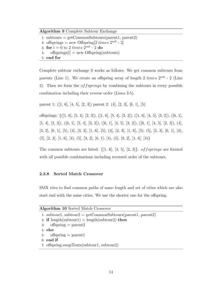
Algorithm 9 Complete Subtour Exchange

1: subtours = getCommonSubtours(parent1, parent2)2: offsprings = new Offspring[2 times 2sub - 2]3: for i = 0 to 2 times 2sub - 2 do4: offsprings[i] = new Offspring(subtours)5: end for

Complete subtour exchange 9 works as follows: We get common subtours from

parents (Line 1). We create an offspring array of length 2 times 2sub - 2 (Line

2). Then we form the offsprings by combining the subtours in every possible

combination including their reverse order (Lines 3-5).

parent 1: ([1, 6], [4, 5], [2, 3]) parent 2: (4], [2, 3], [6, 1], [5)

offsprings: {([1, 6], [5, 4], [2, 3]), ([1, 6], [5, 4], [3, 2]), ([1, 6], [4, 5], [3, 2]), ([6, 1],

[5, 4], [2, 3]), ([6, 1], [5, 4], [3, 2]), ([6, 1], [4, 5], [3, 2]), ([6, 1], [4, 5], [2, 3]), (4],

[3, 2], [6, 1], [5), (4], [3, 2], [1, 6], [5), (4], [2, 3], [1, 6], [5), (5], [2, 3], [6, 1], [4),

(5], [2, 3], [1, 6], [4), (5], [3, 2], [6, 1], [4), (5], [3, 2], [1, 6], [4)}

The common subtours are listed: {[1, 6], [4, 5], [2, 3]}. offsprings are formed

with all possible combinations including reversed order of the subtours.

2.3.8 Sorted Match Crossover

SMX tries to find common paths of same length and set of cities which are also

start end with the same cities. We use the shorter one for the offspring.

Algorithm 10 Sorted Match Crossover

1: subtour1, subtour2 = getCommonSubtours(parent1, parent2)2: if length(subtour1) < length(subtour2) then3: offspring = parent24: else5: offspring = parent16: end if7: offspring.swapTours(subtour1, subtour2)

14

In algorithm 10, we get common paths having properties as stated above (Line 1).

After, we form the offspring from the parent that have longer subtour (Lines

2-5). Then, we swap the subtours to get a shorter path for the offspring.

parent 1: (1, 6, [4, 2, 5, 3]) parent 2: ([4, 5, 2, 3], 1, 6)

offspring: (1, 6, [4, 5, 2, 3])

For these two parents we have two common subtours which are [4, 5, 2, 3] and [4,

2, 5, 3] having lengths 46 and 100 respectively according to distance matrix 3.1.

We use [4, 5, 2, 3] for parent1.

2.4 Mutation

Another important GA operator is the mutation operator. It helps the algorithm

to jump out of the local optima. Various mutation operators have been developed

for TSP, each of which states a local modification of an individual. The operator is

completely blind unless there is a special implementation applied for it. Multiple

mutations and improving mutations are examples of special implementations.

Therefore, diversity is provided by this operator through generations. On the

other hand executing this operator with a small random probability protects

most of the individuals.

In a traditional GA, if we take mutation out of the approach, most probably lots

of applications can no longer produce different individuals after a certain amount

of generations. Here, we present the well-known mutation operators in the TSP

literature in detail. Table 2.2 shows the well-known mutation operators in the

TSP literature.

15

Table 2.2: Well-known mutation operators in the literatureOperator Name PaperExchange Mutation EM [2], [11]Insertion Mutation IM [2], [11]Displacement Mutation DM [2], [11]Simple Inversion Mutation SIM [2]Inversion Mutation IVM [2]Scramble Mutation SM [2]Ends Exchange Mutation ESEM [11]Reverse Ends Mutation RESM [11]Reverse Ends Exchange Mutation RESEM [11]

2.4.1 Reciprocal Exchange Mutation

REM is the classical swap mutation of the traditional GA design. It is shown in

algorithm 11

Algorithm 11 Reciprocal Exchange Mutation

1: function REM(city1 = random(0, N), city2 = random(0, N))2: tour.swap(city1, city2)3: endfunction

We simply select two cities for the function REM (Line 1) and swap them (Line

2).

before: (1, 6, 4, 5, 2, 3)

after: (1, 2, 4, 5, 6, 3)

To apply REM, we swap the cities 6 and 2.

2.4.2 Insertion Mutation

IM 12 is similar to EM rather a city is removed from the tour and inserted into

another randomly chosen place consequently.

A random city’s current and new index are given to the function IM as inputs

(Line 1) and removed from the route (Line 2). At the second stage, the removed

city is inserted into a random place (Lines 3).

16

Algorithm 12 Insertion Mutation

1: function IM(oldIndex = random(0, N), newIndex = random(0, N))2: aCity = tour.removeCity(oldIndex)3: tour.insertCity(newIndex, aCity)4: endfunction

before: (1, 6, 4, 5, 2, 3)

after: (1, 6, 5, 2, 4, 3)

We remove the city 4 from the individual which leads to the subtour [1, 6, 5, 2,

3]. Then, we insert city 4 to a random position of the subtour to form a complete

path.

2.4.3 Displacement Mutation

An extended version of IM is DM where a subroute is exchanged rather than a

single city. It is shown in algorithm 13

Algorithm 13 Displacement Mutation

1: function DM(oldIndex = random(0, N), length = random(0, N), newIndex =random(0, N))

2: aSubtour = tour.removeSubtour(oldIndex, length)3: tour.insertSubtour(newIndex, aSubtour)4: endfunction

For the DM function, we have 3 inputs for displacing a random subtour, (Line

1) which is derived from a starting index and length, is removed from the route

(Line 2). At the second stage, the removed subtour is inserted to the same route

into a random place (Line 3).

before: (1, [4, 6, 5], 2, 3)

after: (1, 2, [4, 6, 5], 3)

We remove the subtour [4, 6, 5] from the tour. We have [1, 2, 3] remained. Then,

we insert subtour [4, 6, 5] into a random position of the individual to form a

complete path.

17

2.4.4 Simple Inversion Mutation

SIM is the reversed version of DM which is described in algorithm 14.

Algorithm 14 Simple Inversion Mutation

1: function SIM(index = random(0, N), length = random(0, N))2: aSubtour = tour.getSubtour(index, length)3: return reverse(aSubtour)4: endfunction

We call SIM with inputs index and length (Line 1). A random subroute which is

obtained from the inputs, selected for reversal (Line 2) and that random subroute

is reversed (Line 3).

before: (1, [4, 6, 5], 2, 3)

after: (1, [5, 6, 4], 2, 3)

We reverse the subtour [4, 6, 5].

2.4.5 Inversion Mutation

IVM 15 is a variation of SIM where reversed subroute is inserted to the route just

like the insertion pattern followed in IM and DM.

Algorithm 15 Inversion Mutation

1: function IVM(oldIndex = random(0, N), length = random(0, N), newIndex= random(0, N))

2: SIM(oldIndex, length)3: DM(oldIndex, length, newIndex)4: endfunction

First, we call the function IVM with input parameters: oldIndex, length, and

newIndex (Line 1). SIM function is invoked to reverse the subtour derived from

oldIndex and length (Line 2). As a final step, we call the function DM to displace

it to newIndex (Line 3).

before: (1, [4, 6, 5], 2, 3)

18

after: (1, 2, [5, 6, 4], 3)

We remove the subtour [4, 6, 5]. Then, place its reversed version [5, 6, 4] into a

random place in the individual.

2.4.6 Scramble Mutation

Scramble Mutation 16 has the maximum number of enhancements according to

the paper [2].

Algorithm 16 Scramble Mutation

1: function SM(index = random(0, N), length = random(0, N))2: aSubtour = tour.getSubtour(index, length)3: return scramble(aSubtour)4: endfunction

First, we call the function SM with index and length inputs (Line 1). Then, by

using these inputs we select a random subtour (Line 2) and scramble it (Line 3).

before: (1, [4, 6, 5], 2, 3)

after: (1, [6, 5, 4], 2, 3)

We scramble the subtour [4, 6, 5] leading [6, 5, 4].

2.4.7 Ends Exchange Mutation

ESEM 17 is similar to DM but we use it twice for the ends of the individual.

Algorithm 17 Ends Exchange Mutation

1: function ESEM(length = random(0, N/2))2: DM(0, length, N)3: DM(N - (length times 2), length, 0)4: endfunction

We invoke ESEM (Line 1). Then, we apply DM to the ends of the individual

with selected length (Lines 2-3).

19

before: ([1, 4], 6, 5, [2, 3])

after: ([2, 3], 6, 5, [1, 4])

We simply swap two subtours [1, 4] and [2, 3] from the ends of the individual.

2.4.8 Reverse Ends Mutation

RESM 18 is similar to SIM but we use it twice for the ends of the chromosome.

Algorithm 18 Reverse Ends Mutation

1: function RESM(length = random(0, N/2))2: SIM(0, length)3: SIM(N - length, N)4: endfunction

We call the function RESM (Line 1). Then, we apply SIM to the ends of the

individual with selected length (Lines 2-3).

before: ([1, 4], 6, 5, [2, 3])

after: ([4, 1], 6, 5, [3, 2])

We reverse the subtours [1, 4] and [2, 3] from the ends of the chromosome.

2.4.9 Reverse Ends Exchange Mutation

RESEM 19 is similar to IVM but we use it twice for the ends of the individual.

The subtour length should be <= N/2.

Algorithm 19 Reverse Ends Exchange Mutation

1: function RESEM(length = random(0, N/2))2: IVM(0, length, N)3: IVM(N - (length times 2), length, 0)4: endfunction

We invoke RESEM (Line 1). Then, we apply IVM to the ends of the individual

with selected length (Lines 2-3).

20

Table 2.3: Well-known local operators in the literatureOperator Name Paper2-Opt [6], [12], [13]3-Opt [7]Lin-Kernighan-Opt [7]Remove Sharp [14]LocalOpt [14]Untwist [15]

before: ([1, 4], 6, 5, [2, 3])

after: ([3, 2], 6, 5, [4, 1])

We both apply reversing and swapping to the subtours [1, 4] and [2, 3].

2.5 Local Operators

If we compare an ordinary tour with the optimum tour, an human eye can easily

detect the local problems in the ordinary tour. After several observations, we are

aware of some common problem patterns, i.e. twisted routes. A local optimiza-

tion, by the name itself, optimizes the route by solving these local problems. A

local optimization with a loss of quality in individual score may serve as a global

mutation operator for the algorithm, so we refer to local operators as global mu-

tations. Table 2.3 shows the well-known local operators in the literature.

2.5.1 2-opt

It is one of the most popular local operators in the literature. 2-opt searches the

best swapping of all dual pairs of the individual.

2-opt algorithm 20 searches the best swapping from all dual pairs of the individual

(Lines 2-3). If the score improves after the swap, 2optSwap is applied and the

shortest tour is decided (Lines 4-6).

21

Algorithm 20 2-opt

1: shortest = length(tour)2: for i = 0 to N - 1 do3: for j = i + 1 to N - 2 do4: newTour = tour.2optSwap([i, i+1], [j, j+1])5: if length(newTour) < shortest then6: shortest = length(newTour)7: end if8: end for9: end for

Algorithm 21 2optSwap

1: function 2optSwap([x1, x2], [y1, y2])2: [x1, x2].cut()3: [y1, y2].cut()4: [x1, y2].merge()5: [x2, y1].merge()6: endfunction

In 2optswap algorithm 21, we invoke 2optSwap with two edge inputs (Line 1).

We cut those 2 edges (Lines 2-3). Then, we merge the cities with the second

possible option (Lines 4-5).

2.5.2 3-opt

It is one of the most popular local operators in the literature. 3-opt searches

the best swapping from all ternary pairs of the individual. 3-opt mechanism is a

version of 2-opt.

In 3-opt algorithm 22, we search for the best ternary pairs (Lines 1-3). At the

second stage, 3optSwap is used to determine the shortest path in the current

iteration (Lines 4-7).

3optSwap algorithm 23 is called with 3 edge parameters (Line 1). The function

is about cutting those 3 edges from the tour (Lines 2-4). Then, the shortest

combination of the edges are merged (Lines 5-6).

22

Algorithm 22 3-opt

1: shortest = length(tour)2: for i = 0 to N - 1 do3: for j = i + 1 to N - 2 do4: for k = j + 1 to N - 3 do5: newTour = tour.3optSwap([i, i+1], [j, j+1], [k, k+1])6: if length(newTour) < shortest then7: shortest = length(newTour)8: end if9: end for10: end for11: end for

Algorithm 23 3optSwap

1: function 3optSwap([x1, x2], [y1, y2], [z1, z2])2: [x1, x2].cut()3: [y1, y2].cut()4: [z1, z2].cut()5: edges = getShortestEdgeCombination(x1, x2, y1, y2, z1, z2)6: edges.merge()7: endfunction

2.5.3 Lin-Kernighan Opt

Lin-Kernighan approach uses path swapping with k-opt technique where k is

determined by the algorithm itself at each iteration. k is mostly 2 or 3.

Algorithm 24 Lin-Kernighan Opt

1: for iterate over all dual or ternary edge pairs do2: apply 2-opt or 3-opt to the tour.3: try all subtour combinations to minimize the tour length.4: end for

In Lin-Kernighan opt algorithm 24, we iterate on all edge pairs (Line 1). After,

we remove 2 or 3 edges from tour (Line 2). These removed edges are said to

be the worst edges of the tour. So, replacing them with feasible subtours will

minimize the tour length (Line 3).

23

2.5.4 Remove Sharp

Remove Sharp removes a city from the tour. Then, the operator inserts the city

into before and after all of its k-nn. The insertion place where the shortest value

in tour length is selected for the tour construction.

Algorithm 25 Remove Sharp

1: function removesharp(city = random(0, N))2: shortest = length(tour)3: aCity = tour.removeCity(city)4: for i = 0 to k do5: tour.insertCity(i, aCity)6: if length(tour) < shortest then7: shortest = length(tour)8: shortestIndex = i9: end if10: tour.removeCity(i, aCity)11: end for12: tour.insertCity(shortestIndex, aCity)13: endfunction

removesharp algorithm 25 takes two parameters (Line 1). The operator removes

a random city from the tour resulting a cyclic path of N − 1 cities (Line 3). The

removed city is inserted into the path before and after the all k-nearest neighbours

of the city to look for which tour gives the shortest path among all (Lines 4-11).

As a last step, we insert the selected city which makes the tour shortest (Line

12).

2.5.5 LocalOpt

LocalOpt selects a subtour from the tour. Then we try all possible combinations

of the tour to construct the shortest one among all combinations.

LocalOpt algorithm 26 takes two inputs (Line 1) to select aSubtour from the tour

(Line 2). We get all possible combinations of the tour to construct a shorter one

(Line 4). The best combination is selected as the shortest path of the cities (Lines

5-10).

24

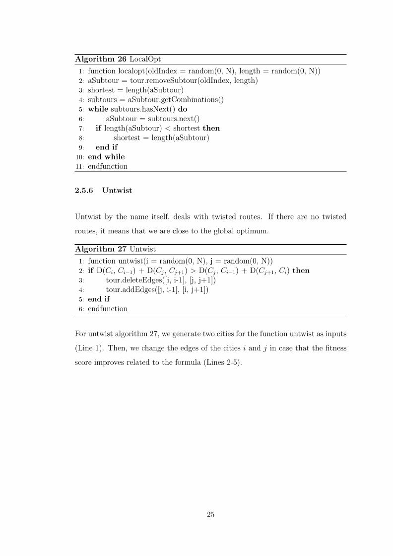
Algorithm 26 LocalOpt

1: function localopt(oldIndex = random(0, N), length = random(0, N))2: aSubtour = tour.removeSubtour(oldIndex, length)3: shortest = length(aSubtour)4: subtours = aSubtour.getCombinations()5: while subtours.hasNext() do6: aSubtour = subtours.next()7: if length(aSubtour) < shortest then8: shortest = length(aSubtour)9: end if10: end while11: endfunction

2.5.6 Untwist

Untwist by the name itself, deals with twisted routes. If there are no twisted

routes, it means that we are close to the global optimum.

Algorithm 27 Untwist

1: function untwist(i = random(0, N), j = random(0, N))2: if D(Ci, Ci−1) + D(Cj, Cj+1) > D(Cj, Ci−1) + D(Cj+1, Ci) then3: tour.deleteEdges([i, i-1], [j, j+1])4: tour.addEdges([j, i-1], [i, j+1])5: end if6: endfunction

For untwist algorithm 27, we generate two cities for the function untwist as inputs

(Line 1). Then, we change the edges of the cities i and j in case that the fitness

score improves related to the formula (Lines 2-5).

25

Chapter 3

Proposed Algorithm

3.1 Greedy k-nn Crossover

Before implementing our special algorithm, we have analyzed how an optimal tour

looks like for a specific data. We observed that in an optimal route two cities

belonging to an edge are closely related in a k-nearest neighbour way. A city C1

is in the k-nn list of city C2; C1 is one of the closest k cities of city C2. Mostly,

we found that, a city is connected to its first, second or third nearest neighbour

in the optimal tour as shown in Table 3.1. So, we have decided to implement a

crossover method to satisfy the k-nn logic. We name this novel crossover method

as greedy k-nn crossover. It is called greedy because we extend the abilities of

the greedy crossover [8], where it provides us a base for our new approach.

Table 3.1: The number of k-nearest neighbours appearing in the optimal tourk/Dataset berlin52 eil51 eil76 eil101 kroa100 pcb4421 42 44 59 83 87 3552 27 32 46 56 46 2943 13 9 28 33 28 1404 6 8 8 13 20 565+ 16 9 11 17 19 39

26

Algorithm 28 Greedy k-nn Crossover

1: city = parent1.getFirstCity()2: offspring.add(city)3: while offspring not complete do4: next1 = parent1.getCity(city).next()5: next2 = parent2.getCity(city).next()6: if !memberOf(offspring, next1) AND !memberOf(offspring, next2) then7: if next1 < next2 then8: offspring.add(next1)9: city = next110: else11: offspring.add(next2)12: city = next213: end if14: else if !memberOf(offspring, next1) then15: nncity = city.knn(4)16: if next1 < nncity then17: offspring.add(next1)18: city = next119: else20: offspring.add(nncity)21: city = nncity22: end if23: else if !memberOf(offspring, next2) then24: nncity = city.knn(4)25: if next2 < nncity then26: offspring.add(next2)27: city = next228: else29: offspring.add(nncity)30: city = nncity31: end if32: else33: nncity = city.knn(4)34: offspring.add(nncity)35: city = nncity36: end if37: end while

27

In greedy k-nn crossover 28, we select the first city of parent1 and add it to the

offspring (Lines 1-2). Then, we iterate until offspring represents a complete tour

(Line 3). At each iteration, we determine the next city in both parents (Lines

4-5). If both of them do not exist in offspring, we compare them with respect

to their edge length (Line 6). The shorter edge will be added to the offspring

and current city is updated for the next iteration (Lines 7-13). If the next city of

parent1 is available only, we compare it with a city derived from k-nn heuristic.

The shorter edge will be added to the offspring and current city is set as before

(Lines 14-22). We do the same process for the condition that only the next city

of parent2 is available (Lines 23-31). If next cities of both parents exist in the

offspring, we simple get a city from k-nn list and update the current city. (Lines

32-36).

Table 3.2: Distance Matrix D

D =

∞ 72 36 12 4 5

72 ∞ 14 89 1 73

36 14 ∞ 6 10 19

12 89 6 ∞ 31 99

4 1 10 31 ∞ 6

5 73 19 99 6 ∞

Let’s say k = 2 and initially we have two parent chromosomes:

parent 1: (1, 6, 4, 5, 2, 3)

parent 2: (4, 2, 3, 6, 1, 5)

According to distance matrix D in Table 3.1, aparent1 has length 274 and parent

2 has 162. First of all, we should have a template which would be the one of parent

28

chromosomes. We select the template chromosome as parent1. So city 1 is the

first city of the offspring.

offspring: [1]

Then, we locate city 1 in both parents to compare the edges that contains it. (1,

6) and (1, 5) are the candidate edges. Since D(1, 5) < D(1, 6), we select edge (1,

5) to add to the offspring.

offspring: [1, 5]

After the offspring’s first two cities are formed, we see that city 5 in parent2 is the

last city. For this crossover model, we represent edges in a left to right manner

because individuals are processed in the same direction. As a result, taking the

first city from a chromosome is the right way to form the edge, if we are trying

to find the edge partner of the last city. Candidate edges are: (5, 2) and (5, 4).

Since D(5, 2) < D(5, 4), we select edge (5, 2) to add to the offspring.

offspring: [1, 5, 2]

Both of the parents have the same edge going out from 2, so we have one candidate

edge to select from: namely (2, 3).

offspring: [1, 5, 2, 3]

Edges that contains the city 3 are (3, 1) and (3, 6). The city 1 is already in the

offspring. So, our k-nn model steps into the hybrid crossover design. 2-nn of city

3 is 4, 5. City 5 exists in the offspring so we pick city 4 and compare edges

(3, 4) and (3, 6). Since D(3, 4) < D(3, 6), we select edge(3, 4) to add to the

offspring.

offspring: [1, 5, 2, 3, 4]

There are two edges going out from city 4: (4, 2) and (4, 5). Both cities 2 and 5

are in the offspring. So we use k-nn model to pick a city. There is one suitable

29

city left to put into the offspring, so k-nn will choose that city as expected.

Complete offspring with length 129 is as follows:

offspring: (1, 5, 2, 3, 4, 6)

3.2 Greedy Selection

RWS and TS are the popular selection methods as described in Chapter 2. But

initialization of the population with those selection methods result in a chromo-

some list full of cities having nearly equal scores with these methods. So when

selecting cities from the population, we see that best chromosome and worst

chromosome do not differ so much.

Algorithm 29 Greedy Selection

1: initialize population2: while termination do3: value = random(0, 1)4: exp = power(value, 4)5: index = exp * populationSize6: return index7: end while

As a result, we have implemented a simple selection method named greedy se-

lection as shown in algorithm 29. First, we get a random value between 0 and

1 (Line 3). Then, we calculate value 4 so that we select better chromosomes

(Line 4). Finally, we multiple the value with population size to indicate its in-

dex (Line 5). Sorting of individual fitness scores is required for this method to

work successfully. This design provides fitter chromosomes to be selected more

frequently.

3.3 Extended Untwist

We are using this formula for every city pair in an individual rather than selecting

one pair in the classical one. This kind of processing reminds us 2-opt. Untwisting

30

a route may result in worse paths or can lead to a more twisted route exclusively

in early generations. We tweak local operator untwist, to take more advantage of

it.

Algorithm 30 Extended Untwist

1: for i = 0 to N - 1 do2: for j = i + 1 to N do3: untwist(i, j)4: end for5: end for

Untwist by the name itself, deals with twisted routes. We extend the abilities of

this operator by applying this formula to all dual city pairs in a complete tour

(Lines 1-2) as shown in algorithm 30.

3.4 Other Elements

We choose REM as the mutation element for our system. Our mutation rate is

10%. The best individual survives to the next generation for survival strategy

and 10% of the population is replaced with newly created artificial chromosomes

to maintain the diversity through the iterations. These chromosomes are called

reinforcements. We take k as 5 through the algorithm. By doing this, the system

moves around good paths to approach the global optimum.

According to our preliminary results, the best individual of the population occa-

sionally is not sufficient for a good result. In most of the populations, the best

individual have some good and bad parts unless we have successfully approached

global optimum. So, we have decided to work with multiple populations. At

specific generation intervals, we immigrate the best individuals of all populations

to other populations. By doing this, we make all populations collaborate together

to reach the optimum route.

3.5 The Algorithm

31

Algorithm 31 Proposed Hybrid GA

1: population = new Population(populationSize)2: while generation < numberOfIterations do3: newPopulation.add(population.best())4: chromosomes = population.greedyknn(greedyselection(), k)5: newPopulation.add(chromosomes)6: newPopulation.reinforcement(k, reinforcementRate)7: if probability <= mutationRate then8: chromosome.REM()9: end if10: chromosome.extendedUntwist()11: newPopulation.evaluate()12: best = population.best()13: population = newPopulation14: end while

We present our novel algorithm in algorithm 31. We initiate our population

with k-nn approach (Line 1). We do numberOfIterations (Line 2). At each

iteration we protect the best individual from previous population (Line 3) and

add reinforcements with 10% rate. After, we mutate an individual with 10%

probability (Lines 7-9). Extended untwist is applied to all chromosomes (line

10). Finally, we evaluate the population to determine the fittest individual (Lines

11-12) and clone newPopulation to serve for the next generation (Line 13).

32

Chapter 4

Experiments

4.1 Experimental Setup

In order to compare our work with previous approaches we select the datasets

that are frequently used in the literature. The datasets that we use are, berlin52,

eil51, eil76, eil101, kroa100, and pcb442. The tests are performed on a commodity

computer; RAM: 8 GB and CPU: 2.40Ghz * 4.

We run our algorithm 10 times and compare out results with the optimum tours

[16].The algorithm parameters are given in the Table 4.1.

4.2 Experimental Results

Table 4.1: Algorithm Parametersk 5populationSize 200populationCount 4crossoverRate 100%mutationRate 10%reinforcementRate 10%numberOfIterations 10000

33

Table 4.2: Experimental ResultsDataset Optimum Best Error (%) Average Error (%)berlin52 7544.36 7544.36 0 7544.36 0eil51 428.87 428.87 0 428.89 0.004eil76 544.36 544.36 0 544.36 0eil101 640.21 640.21 0 641.66 -0.09kroa100 21285.44 21285.44 0 21285.44 0pcb442 50783.54 51036.06 0.49 51159.53 0.74

Table 4.3: Experimental Results with one populationDataset Optimum Best Error (%) Average Error (%)berlin52 7544.36 7544.36 0 7544.36 0eil51 428.87 428.87 0 428.90 0.006eil76 544.36 544.36 0 544.81 0.08eil101 640.21 640.21 0 643.50 0.51kroa100 21285.44 21285.44 0 21287.63 0.02pcb442 50783.54 na na na na

Table 4.4: Experimental Results with PMXDataset Optimum Best Error (%) Average Error (%)berlin52 7544.36 7544.36 0 7544.36 0eil51 428.87 428.87 0 428.88 0.002eil76 544.36 544.36 0 547,79 0.63eil101 640.21 646.57 0.99 650.03 1.53kroa100 21285.44 21285.44 0 21291.70 0.02pcb442 50783.54 na na na na

According to the experimental results shown in the Table 4.2, we reach the opti-

mum tour in small datasets but in bigger datasets we are close to optimum.

According to the experimental results with one population in Table 4.3, multiple

population model outperforms in average tour quality of the dataset eil101. In

smaller datasets,

34

Table 4.5: Experimental Results with k = 1Dataset Optimum Best Error (%) Average Error (%)berlin52 7544.36 7544.36 0 7544.36 0eil51 428.87 428.87 0 428.91 0.009eil76 544.36 544.36 0 544.76 0.07eil101 640.21 642.05 0.28 643.08 0.44kroa100 21285.44 21285.44 0 21285.44 0pcb442 50783.54 50966.08 0.35 50966.08 0.35

Table 4.6: Experimental Results with TSDataset Optimum Best Error (%) Average Error (%)berlin52 7544.36 7544.36 0 7544.36 0eil51 429.98 428.87 0 428.87 0eil76 544.36 544.36 0 545.69 0.24eil101 640.21 643.44 0.50 648.20 1.09kroa100 21285.44 21285.44 0 21288.53 0.01pcb442 50783.54 53174.66 4.70 53174.66 4.70

According to the experimental results with PMX in Table 4.4, our novel crossover

operator is superior especially in the datasets eil76 and eil101. In smaller datasets,

both crossovers can reach the optimum tour.

According to the experimental results with k = 1 in Table 4.5, pcb442 has a good

enhancement in tour length. In smaller datasets, we end up with the optimum

tour or a closer one.

According to the experimental results with TS in Table 4.6, our novel greedy

selection method performs much better than the popular TS in the datasets

pcb442 and eil101. In smaller datasets, the difference in tour quality is slightly

less.

35

Chapter 5

Conclusion

We observe that most of the attempts in the TSP literature come up with a

hybrid design or introduce a new element such as a novel crossover or mutation.

These structures are usually designed to get out of the local optima.

In this thesis, we propose a new selection method and a crossover operator, based

on successful elements from the literature. Our crossover operator decreases the

search space by using k-nn logic. We also extend the abilities of the untwist local

operator. The best individual is protected to the next generation with a survival

selection method. While this helps us to approach the global optimum, reinforce-

ment of artificial chromosomes stabilize diversity level at each generation. We

see that, among multiple populations the best individuals end up with different

routing structures. As a result, we immigrate the best individual of a population

to other populations at specific generations.

We have collected a subset of the popular datasets used in the literature. Our

experimental results show that, proposed novel operators outperform their equiv-

alents in the TSP literature. Multiple population design is superior to its single

version in terms of tour length. With multiple populations, we get to the global

optimum more frequently especially when the number of cities is not large.

Our hybrid approach model, that we presented have, forms a basis to our future

work. In the future, we plan to integrate dynamic behaviour into the structure.

36

At runtime, operators will change according to the diversity level and individual

quality of the population. For the datasets that have large number of cities, we

plan to integrate a route changing plan for the good tours that are trapped in a

local optima.

37

References

[1] CONCORD TSP SOLVER. http://www.math.uwaterloo.ca/tsp/concorde.html.

[2] R.H. Murga I. Inza P. Larranaga, C.M.H. Kuijpers and S. Dizdarevic. Ge-

netic algorithms for the travelling salesman problem: A review of represen-

tations and operators. Artificial Intelligence Review, 13:129–170, 1999.

[3] Otman Abdoun and Jaafar Abouchabaka. A comparative study of adaptive

crossover operators for genetic algorithms to resolve the traveling salesman

problem. International Journal of Computer Applications, 31:49–57, 2011.

[4] L. Darrell Whitley, Timothy Starkweather, and D’Ann Fuquay. Scheduling

problems and traveling salesmen: The genetic edge recombination operator.

In Proceedings of the 3rd International Conference on Genetic Algorithms,

pages 133–140, 1989.

[5] Y.-F. Tsai H.-K. Tsai, J.-M. Yang and C.-Y. Kao. Some issues of designing

genetic algorithms for traveling salesman problems. Soft Computing, 8:689–

697, 2004.

[6] K. Ghoseiri and H. Sarhadi. A 2opt-dpx genetic local search for solving sym-

metric traveling salesman problem. Industrial Engineering and Engineering

Management, 2007 IEEE International Conference on, pages 903–906, 2007.

[7] Bernd Freisleben and Peter Merz. A genetic local search algorithm for solving

symmetric and asymmetric traveling salesman problems. Evolutionary Com-

putation, 1996., Proceedings of IEEE International Conference on, pages

616–621, 1996.

38

[8] Sushil J. Louis and Gong Li. Case injected genetic algorithms for traveling

salesman problems. Information Sciences, 122:201–225, 2000.

[9] H. Sakamoto H. K. Katayama and Narihisa. The efficiency of hybrid mu-

tation genetic algorithm for the travelling salesman problem. Mathematical

and Computer Modelling, 31:197–203, 2000.

[10] Kengo Katayama and Hiroyuki Narihisa. An efficient hybrid genetic algo-

rithm for the traveling salesman problem. Electronics and Communications

in Japan, 84:76–83, 2001.

[11] Saleem Zeyad Ramadan. Reducing premature convergence problem in ge-

netic algorithm: Application on travel salesman problem. Computer and

Information Science, 6:47–57, 2012.

[12] Lijie Li and Ying Zhang. An improved genetic algorithm for the traveling

salesman problem. Communications in Computer and Information Science,

2:208–216, 2007.

[13] Hongwei Dai Yu Yang and Changhe Li. Adaptive genetic algorithm with

application for solving traveling salesman problems. Internet Technology

and Applications, 2010 International Conference on, pages 1–4, 2010.

[14] G. Andal Jayalakshmi, S. Sathiamoorthy, and R. Rajaram. A hybrid genetic

algorithm - a new approach to solve traveling salesman problem. Interna-

tional Journal of Computational Engineering Science, 2:339–355, 2001.

[15] Jie Zhang Li-ying Wang and Hua Li. An improved genetic algorithm for

tsp. Machine Learning and Cybernetics, 2007 International Conference on,

2:925–928, 2007.

[16] TSPLIB95. http://comopt.ifi.uni-heidelberg.de/software/tsplib95/.

39

Curriculum Vitae

Cengiz Asmazoglu was born in 05 August 1983, in Istanbul. He received his B.S.

degree in Computer Engineering in 2010 from Isık University. His research inter-

ests include optimization algorithms, artificial intelligence, information retrieval

and data mining.

40