An exploratory factor analysis of visual performance in a large population

Article (Accepted Version)

http://sro.sussex.ac.uk

Bosten, J M, Goodbourn, P T, Bargary, G, Verhallen, R J, Lawrance-Owen, A J, Hogg, R E and Mollon, J D (2017) An exploratory factor analysis of visual performance in a large population. Vision Research, 141. pp. 303-316. ISSN 0042-6989

This version is available from Sussex Research Online: http://sro.sussex.ac.uk/id/eprint/67012/

This document is made available in accordance with publisher policies and may differ from the published version or from the version of record. If you wish to cite this item you are advised to consult the publisher’s version. Please see the URL above for details on accessing the published version.

Copyright and reuse: Sussex Research Online is a digital repository of the research output of the University.

Copyright and all moral rights to the version of the paper presented here belong to the individual author(s) and/or other copyright owners. To the extent reasonable and practicable, the material made available in SRO has been checked for eligibility before being made available.

Copies of full text items generally can be reproduced, displayed or performed and given to third parties in any format or medium for personal research or study, educational, or not-for-profit purposes without prior permission or charge, provided that the authors, title and full bibliographic details are credited, a hyperlink and/or URL is given for the original metadata page and the content is not changed in any way.

1

An exploratory factor analysis of visual performance in a large population

Bosten JM1, Goodbourn PT2, Bargary G3, Verhallen RJ3, Lawrance-Owen AJ3, Hogg

RE4 and Mollon JD3 1School of Psychology, University of Sussex; J.Bosten@sussex.ac.uk. 2School of Psychological Sciences, The University of Melbourne. 3Department of Psychology, University of Cambridge. 4Centre for Vision Science and Vascular Biology, Queen’s University Belfast.

A factor analysis was performed on 25 visual and auditory performance measures

from 1060 participants. The results revealed evidence both for a factor relating to

general perceptual performance, and for eight independent factors that relate to

particular perceptual skills. In an unrotated PCA, the general factor for

perceptual performance accounted for 19.9% of the total variance in the 25

performance measures. Following varimax rotation, 8 consistent factors were

identified, which appear to relate to (1) sensitivity to medium and high spatial

frequencies, (2) auditory perceptual ability (3) oculomotor speed, (4) oculomotor

control, (5) contrast sensitivity at low spatial frequencies, (6) stereo acuity, (7)

letter recognition, and (8) flicker sensitivity. The results of a hierarchical cluster

analysis were consistent with our rotated factor solution. We also report

correlations between the eight performance factors and other (non-performance)

measures of perception, demographic and anatomical measures, and

questionnaire items probing other psychological variables.

Individual differences, factor analysis, vision, audition, psychophysics, cluster

analysis, contrast sensitivity, eye movements, stereopsis, personality

Introduction

Different individuals perceive the world differently from one another. These

differences may arise from inherited variations in the structure of the visual and

auditory systems or from variations in experience during an individual’s lifetime.

Variations in human perception have been perhaps less studied than variations in

cognitive skills. However, not only do they have significant impact on our behaviour

but they also offer a powerful method of analysing perceptual mechanisms (Kanai &

Rees, 2011; König & Dieterici, 1892; Peterzell, 2016; Wilmer, 2008).

Whenever visual or auditory performance is measured in a sample of participants, there

is variance evident in the data. This variance comes from three sources: (i) instrumental

and other measurement error, (ii) within-individual variation (e.g. temporal fluctuations

in motivation and arousal), and (iii) between-individual variation, i.e. persisting

differences between participants caused by between-individual variation in processes

underlying perceptual functions. To demonstrate true between-individual differences it

is necessary to show one or both of two types of result. First, one may show a significant

test-retest reliability for the trait of interest (Spearman, 1904b; Wilmer, 2008). Second,

one can demonstrate a significant correlation between the trait of interest and another,

independent, phenotypic or genotypic measure (Kanai & Rees, 2011; Wilmer, 2008).

Correlational methods can be successfully used to analyse the mechanisms that underlie

traits of interest. A classical example in vision was the identification of the genetic

polymorphisms that underlie colour vision deficiency and that also contribute to the

2

normal variation in Rayleigh matches (Nathans, Piantanida, Eddy, Shows, & Hogness,

1986; Winderickx et al., 1992). More recently, genome-wide association has been

applied to variation in visual performance in the PERGENIC cohort, whose data are the

basis of the present paper: Correlations have been found between genetic

polymorphisms and hetereochromatic flicker photometric settings (Lawrance-Owen et

al., 2014), phorias (Bosten et al., 2014), face detection (Verhallen et al., 2014) and

sensitivity to ‘frequency-doubled’ gratings (Goodbourn et al., 2014). In another fruitful

use of the correlational method, relationships have been discovered between the size of

cortical structures and visual performance on a range of tasks, including visual acuity

(Duncan & Boynton, 2003), orientation sensitivity (Song, Schwarzkopf, & Rees, 2013),

susceptibility to geometric illusions (Schwarzkopf, Song, & Rees, 2011) and rate of

perceptual rivalry (Kanai, Bahrami, & Rees, 2010).

A celebrated approach to the analysis of correlations is factor analysis (Mulaik, 2009;

Spearman, 1904a, 1927; Thurstone, 1931). Factor analysis aims to discover whether a

smaller set of underlying unobserved variables – known as factors – are responsible for

the intercorrelations between a set of observed variables. The meanings of any factors

revealed by factor analysis are open to interpretation, but in psychology they have often

been thought to relate to the psychological processes that determine the variation in the

observed data.

Factor analysis has been comprehensively applied in the field of cognition, to address

the question of whether cognitive ability is determined by a set of independent factors

or whether it is determined by a single underlying factor, Spearman’s g (Mackintosh,

2011; Spearman, 1904a; Thurstone, 1944). For vision, an equivalent question is

whether the observed variation in performance on a battery of visual tasks is determined

for each task separately, or whether it is determined by a single underlying factor or

small set of factors,

Several studies have applied factor analysis to perception. An early example was the

analysis of 22 auditory tests by Karlin (1942). Particularly celebrated is the study of

Thurstone (1944), who administered 40 tests to 194 subjects. Most of the tests were

visual, including some measures of “low-level” visual processes such as dark

adaptation, peripheral span and flicker fusion, and many tests of “high-level” processes

such as Necker cube rivalry, various geometric illusions, Gestalt figure completion,

colour-form memory, block design and the Gottschaldt figures. Also included were

some non-visual tests, including reaction time to an auditory tone, social judgement and

a test of social influence. Thurstone cautioned that his study was exploratory and

required confirmation by future studies, but he found 11 factors, the first seven of which

he interpreted as perceptual closure, susceptibility to geometric illusions, reaction time,

perceptual alternation, ability to manipulate two alternative mental processes,

perceptual speed and general intelligence.

Since Thurstone’s study, researchers have applied factor analysis to a range of visual

tasks, but they generally have been concerned with particular aspects of visual

perception. A good example is provided by Peterzell and Teller’s studies of spatial,

temporal and chromatic contrast sensitivity (Dobkins, Gunther, & Peterzell, 2000;

Peterzell & Teller, 1996; Peterzell & Teller, 2000; Peterzell, 2016), which have

supported the idea that sets of distinct visual factors underlie contrast sensitivity

functions. In the domain of colour, factor analysis has been used to investigate

3

sensitivity as a function of wavelength (Jones, 1948; Jones & Jones, 1950), to test the

independence of the cardinal colour mechanisms (Gunther & Dobkins, 2003), to

explore the sources of individual variation in colour matching (MacLeod & Webster,

1983), to investigate wavelength discrimination (Diener, 1986; Pickford, 1962), and to

explore sources of variation in tests for colour vision deficiency (Aspinall, 1974). Other

authors have examined measures of perceptual closure (Beard, 1965; Keehn, 1956;

Mooney, 1954; Thurstone, 1950; Wasserstein, Barr, Zappulla, & Rock, 2004).

A smaller number of studies have followed Thurstone (Thurstone, 1950; Thurstone,

1944) in using factor analysis (or the related method of principal components analysis;

PCA) to study the factors underlying variation in a large range of visual abilities. For a

group of 20 participants, Halpern et al. (1999) made measurements of orientation

discrimination, wavelength discrimination, contrast sensitivity, vernier acuity, motion

direction discrimination, velocity discrimination and identification of complex forms.

They observed many significant intercorrelations between the tests, and concluded,

using PCA, that a single factor (accounting for 30% of the total variance) predicts a

portion of the variance on each test apart from discrimination of motion direction.

For a group of 40 participants, Cappe et al. (2014) applied PCA to measurements of

visual acuity, vernier acuity, backward masking, contrast sensitivity and bisection

discrimination. They emphasised the low correlations between pairs of tasks, with only

four significant correlations, for which shared variance ranged between 10 and 30%

(Test-retest reliabilities for individual tasks were not reported, however). Using PCA,

they found that one factor explained 34% of the total variance. However, they applied

a different criterion to that of Halpern et al. (1999) in deciding how much variance a

common factor must explain, concluding that 34% shared variance was not evidence

for a single factor underlying the intercorrelations between visual tests.

In a study of 101 normal participants, Ward et al. (2016, published in the current special

issue of Vision Research) obtained data for seven visual tasks: detection of gabors,

contrast sensitivity, detection of Glass patterns, detection of coherent motion, visual

search, detection of curvature and judgement of temporal order. They applied a factor

analysis to test the hypothesis that there are two visual factors that reflect the activity

of the parvocellular and magnocellular systems. They found two components, which

accounted for 19% and 18% of the total variance. Tasks involving high spatial

frequencies generally loaded on the first component, and tasks involving low spatial

frequencies on the second. The authors concluded that this was compatible with a

magnocellular–parvocellular distinction.

The present study continues the tradition of Thurstone (1944) and those who have

followed, in applying factor analysis to a range of visual tasks to explore the underlying

causes of individual variation in visual ability. We do this on a much larger sample (n

= 1060) than has been used previously, and we include 25 visual, oculomotor and

auditory measures. Our primary analysis is an exploratory factor analysis; and we

demonstrate the reliability of the analysis by showing that very similar factors emerge

if the total cohort is randomly divided into two subsets of participants. We also show

that a comparable structure is recovered when the data are entered into a hierarchical

cluster analysis. In a further analysis, we correlate factor scores with additional

measures gathered from questionnaires (e.g. personality and Autism Quotient), with

4

subjective (non-performance) measures of visual function, and with demographic and

anatomical measures (e.g. sex, iris colour and digit ratio).

Methods

Participants

1060 participants (647 female) took part in the PERGENIC study (e.g. Goodbourn et

al., 2012; Lawrance-Owen et al., 2013). Their ages ranged from 16-40 (mean 22.1; s.d.

4.1). They were recruited from the Cambridge area, and many were students at the

University of Cambridge. Participants were paid £25 for taking part. A subset of 105

participants were selected at random to return for a second testing session on a different

day, an average of 26.4 days (s.d. 23.3 days) after their first, allowing us to measure

test-retest reliabilities. All participants in our sample were of self-reported European

origin.

The study was approved by the Cambridge Psychology Research Ethics Committee and

was carried out in accordance with the tenets of the Declaration of Helsinki. All

participants gave written informed consent before taking part.

Questionnaires

All participants completed a 75-item online questionnaire before they attended the lab

for testing. The questionnaire included items to gather demographic information

(including age, sex, educational level and ancestry) and the mini International

Personality Item Pool-Five-Factor Model (mini-IPIP) to measure the ‘Big 5’

personality traits of extraversion, imagination, agreeableness, conscientiousness and

neuroticism (Donnellan, Oswalk, Baird, & Lucas, 2006). We included various items

intended to assess visual and auditory ability, physical ability, memory and handedness

– abilities that we considered may impact performance on visual and auditory

psychophysical tests. We included three items intended to measure synesthetic

experience. In our analysis, data from the three items were collapsed into one total

synaesthesia score.

The items that will be discussed in this paper are listed in Table 1. For each item,

participants were required to rate their agreement with a statement on a Likert scale

ranging from 1 (strongly disagree) to 5 (strongly agree). Additional items were included

to record the extent of a participant’s computer and video game use, and amount of

musical experience.

A subset of 555 participants completed a second online questionnaire about 6 months

after completing the psychophysical tests. The second questionnaire included a set of

50 items to measure the Autism Quotient (Baron-Cohen, Wheelwright, Skinner,

Martin, & Clubley, 2001), items to measure history of smoking and alcohol use, and

items to measure GCSE score. The latter is a number that quantifies performance in

nationally moderated exams that UK school children sit at age 16. Our motivation for

including the GCSE measure is that it has been found to correlate highly with general

intelligence (Deary, Strand, Smith, & Fernandes, 2007).

I often forget things that have happened in the past that others remember

I have a photographic memory

I can remember the exact shade of a colour several days after seeing it

I find it difficult to hear and produce sounds in foreign languages that are different from my native language

I am good at dancing

I am generally good at sport

5

I am good at ball sports

I always use my right hand when writing

I always throw a ball with my right hand

I make decisions quickly and easily

In my mind’s eye, particular numbers or letters or words always have a particular colour

When I think of the days of the week or the months of the year, I see them laid out in a pattern in space

When I hear, smell, taste or touch something, it evokes an impression in a different sense (e.g. musical notes evoke

specific colours)

I have a natural talent for music

I have absolute or perfect pitch

Table 1 list of questionnaire items considered in this paper

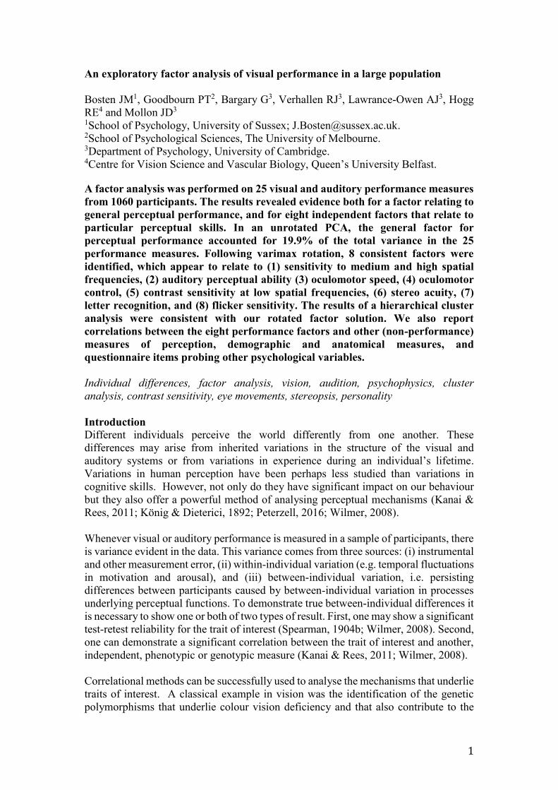
Psychophysical and optometric tests, and anatomical measurements

Participants attended the lab for optometric and psychophysical assessment lasting

approximately 2.5 hours. The sessions were run as a steeplechase in 6 different rooms,

with each participant following the next at 40-minute intervals. There was a break of

about 20 minutes in the middle of the session. Tests in the first testing room were those

requiring administration by an experimenter. In subsequent rooms participants were

tested automatically with instructions appearing on the computer screens, but an

experimenter was always on call if the participant had questions or if the participant

failed to perform adequately on initial practice trials. A list showing the order of tests

in the battery is provided in Table 2. For many tests, methods have already been

published elsewhere, and in these cases the citation is given in the table. Methods for

tests that have not already been published are included in the present method section.

Participants were corrected to best optical acuity at the beginning of the testing session,

and 234 participants were given lenses to wear because their acuity was improved by

at least 0.1 LogMAR with the addition of the correction. Visual acuity was recorded

before and after the additional correction was given.

Room 1

Visual acuity (corrected* and with usual correction only)

Pelli-Robson contrast sensitivity* Pelli, Robson and Wilkins, (1988); Bosten et al. (2015)

Ishihara Plates (5 plates) Lawrence-Owen et al. (2014)

OSCAR test Lawrence-Owen et al. (2014)

TNO stereo acuity* Bosten et al. (2015)

Horizontal and vertical near and far phorias Bosten et al. (2014)

Pupil size Bosten et al. (2015)

Iris colour

Digit ratio Lawrence-Owen et al. (2013)

MPOD macular pigment density

MPOD critical flicker fusion*

Room 2

Coherent motion* Goodbourn et al. (2012)

Ambiguous motion

Coherent form (Glass patterns* and sine wave*) Bosten et al. (2015)

Contrast sensitivity for ‘frequency-doubled’ gratings* Goodbourn et al. (2012)

Room 3

Contrast sensitivity on pulsed* and steady* pedestals Goodbourn et al. (2012); Bosten et al. (2015)

Sensitivity to S-cone increments and decrements* Goodbourn et al. (2012); Bosten et al. (2014)

Simultaneous lightness contrast

Simultaneous colour contrast

Rivalry for ambiguous figures: Necker cube

Rivalry for ambiguous figures: Duck-rabbit

Room 4

Binocular rivalry Bosten et al. (2015)

Dichoptically masked* and unmasked* contrast sensitivity

for gratings of 3 c.p.d.

Bosten et al. (2015)

Crossed and uncrossed stereo acuity* Bosten et al. (2015)

Vernier acuity*

6

Room 5

Main sequence* Bargary et al. (n.d.)

Pro-saccadic latency* Bargary et al. (n.d.)

Latency variability* Bargary et al. (n.d.)

Express saccades* Bargary et al. (n.d.)

Anti-saccade error rate* Bargary et al. (n.d.)

Anti-saccade latency* Bargary et al. (n.d.)

Smooth pursuit RMSE* Bargary et al. (n.d.)

Room 6

Auditory frequency sensitivity* Bosten et al. (2015)

Auditory duration sensitivity* Bosten et al. (2015)

Sensitivity to auditory temporal order* Goodbourn et al. (2012)

Follow up tests online

Glasgow face matching test Verhallen et al. (2017)

Cambridge face memory test Verhallen et al. (2017)

Composite face test Verhallen et al. (2017)

Mooney face test Verhallen et al. (2017)

Table 2. Psychophysical tests in the order that they were run. If methods have been

published previously, the citation is provided. If methods have not been previously

published, details can be found in the present Methods section. Asterisks indicate the

measures that were included in our primary analyses.

Iris colour

To measure objectively the lightnesses, chromaticities and chromatic variances of

participants’ irises we imaged participants’ eyes using a digital camera under controlled

lighting conditions. We used a Canon EOS 1000D digital camera fitted with a Tamron

A15 telephoto lens and a Sigma EF-530 DG ST flash, positioned 1.2 m from

participants’ eyes. The aperture value was F5, the exposure time was 5 ms, the ISO

speed was 100, and the focal length was 171 mm. Participants viewed a CRT monitor

displaying a blank grey field of luminance 35 cd.m-2 and chromaticity CIE x=0.29, y =

0.32. Images of the eyes were captured through a rectangular aperture in a piece of

white card perpendicular to the camera’s line of view. Displayed on the white card was

an array of Kodak colour patches, which allowed us to colour calibrate the images using

measurements of the same patches made by a SpectraScan PR650 spectroradiometer.

The average colour, average lightness and average variance of each participant’s iris

were extracted using the (linear) raw images, colour calibrated by accounting for the

camera’s spectral sensitivity functions (which we measured using a set of 31

interference filters peaking at 10 nm intervals between 400 and 700 nm), and the RGB

values of the Kodak colour patches in each image (See Lawrance-Owen, 2012 for more

detailed methods).

Macular pigment density and peripheral and central critical flicker frequencies

Macular pigment density was estimated using the MPOD (Tinsley Precision

Instruments Ltd., Braintree, UK). The MPOD measures the point of minimum flicker

sensitivity as a function of ratio of blue (460 nm) to green (540 nm) light (Murray &

Carden, 2008; Van Der Veen et al., 2009). It makes separate estimates for central and

peripheral viewing, and macular pigment density is estimated using the difference

between the two minima. For extracting minima, we replaced the MPODs default fits

with our own custom fits to the raw data. As part of the MPODs pre-testing routine

measures of central and peripheral CFF (critical flicker fusion frequency) are made, on

the basis of the mean of five settings (Van Der Veen et al., 2009).

Simultaneous contrast (colour and lightness)

7

Colour. On each trial, a grey reference disc of diameter 1º embedded in a coloured

annular surround of 4º was presented on one side of a central (0.1º × 0.1º) grey fixation

cross, at an eccentricity of 2.5º. The disc was metameric with equal energy white, and

had a luminance of 28 cd.m-2. The surround was isoluminant with the reference disc

and had a chromaticity of L/(L+M) = 0.629 and S/(L+M) = 0.016 in the MacLeod–

Boynton (1979) chromaticity diagram. Between the reference disc and the surround

was a black line of thickness 0.05º. On the other side of the fixation cross, also at an

eccentricity of 2.5º, was presented a test disc of diameter 1º, isoluminant with the

reference stimulus and with a chromaticity that varied according to the participant’s

responses. The surround to reference and test stimuli was dark.

The side of presentation of the test and reference stimuli was decided at random on each

trial. The participant’s task was to identify which of the two small discs appeared

redder. The S/(L+M) value of the test disc was 0.016, and the L/(L+M) value was

decided on each trial by two randomly interleaved ZEST staircases (King-Smith et al.

1994; Watson & Pelli, 1983) with starting L/(L+M) values of 0.641 and 0.689. There

were 72 trials, 36 for each staircase.

Luminance. The spatial characteristics of the stimuli for simultaneous luminance

contrast were the same as those for simultaneous colour contrast. The luminance of the

reference disc was 69.2 cd.m-2, and the luminance of the surround was 138.4 cd.m−2.

The luminance of the test disc was decided on each trial by two randomly interleaved

ZEST staircases with starting luminances of 89.1 cd.m−2 and 49.3 cd.m−2. Test and

reference stimuli were themselves presented on a matrix of random luminance noise,

with square 0.06º × 0.06º pixels. The luminance noise was binary at 13.8 cd.m−2 and

124.6 cd.m−2. For simultaneous luminance contrast the procedure was analogous to that

for simultaneous colour contrast, but the participant had to choose on each trial the

lighter disc.

For both simultaneous colour contrast and simultaneous luminance contrast, a

participant’s point of subjective equality was defined as the 50% point on the

psychometric function, where the test and reference discs were equally likely to be

judged as redder (or lighter).

Rivalry for ambiguous figures

We measured the rate of percept alternation for two ambiguous figures: the Necker

cube (Necker, 1832) and a version of the duck-rabbit ambiguous figure (Kihlstrom,

2012). The Necker cube was white, presented on a black background. The two square

faces of the Necker cube were approximately 2º × 2º. The duck-rabbit stimulus was a

greyscale image of 6º (horizontal) × 5º (vertical).

For the Necker cube, participants were instructed to maintain fixation on a central (0.1º

× 0.1º) white cross, and for the duck-rabbit stimulus, they were instructed to maintain

fixation on the eye. Participants were instructed to press a button whenever their percept

changed, either from duck to rabbit in the case of the duck-rabbit figure, or from one

conformation to the other for the Necker cube. Responses were gathered over a period

of 2 minutes for each stimulus using a CT3 response box (Cambridge Research

Systems, Rochester, UK).

8

For the duck-rabbit stimulus, pilot testing revealed that a minority of participants did

not spontaneously see both interpretations of the stimulus. We therefore presented

participants with the stimulus before the testing period started, and instructed them to

alert the experimenter if they could not see both animals.

Vernier acuity

The stimuli for measuring vernier acuity were three white anti-aliased vertical lines (1

× 8 minutes of arc), offset vertically by 4 minutes of arc. The central line was offset

horizontally from the upper and lower lines by a variable distance decided according to

a staircase procedure. The luminance of the lines was 100 cd.m−2, and that of the 2.5º

× 1.8º background was 11 cd.m−2. The stimuli were presented on a Trinitron

Multiscan17seII CRT monitor (Sony, Tokyo, Japan), and the image was reflected in a

mirror to give a total viewing distance of 7.3 m. Responses were gathered using a CT3

response box.

On each trial the stimuli were displayed for 150 ms, followed by the background alone

until participants made a response. Participants were instructed to judge the direction

of displacement of the central line relative to the upper and lower lines, and to press a

button accordingly. Thresholds were measured using four randomly interleaved 3-up

1-down staircases. The starting position for two of the staircases placed the central line

100 seconds of arc to the left of the upper and lower lines (and left was defined as a

correct response). The starting position for the other two staircases placed it 100

seconds of arc to the right of the upper and lower lines (and right was defined as a

correct response). The initial step size for each staircase was 40 seconds of arc. This

reduced to 20 seconds of arc following 4 reversals, and then to 10 seconds after 8

reversals. Each staircase terminated following 10 reversals.

Psychometric functions were fitted to the trial-by-trial data from each pair of staircases

using the local linear fit functions from the Matlab toolbox Modelfree (Zychaluk &

Foster, 2009). The 81% points on each of the two psychometric functions (PL(81) and

PR(81) from the left-starting and right-starting staircases, respectively) were extracted.

Bias was defined as

,

yielding a measure of lateral bias in response independent of threshold. Threshold was

defined as

yielding a measure of vernier threshold independent of bias.

The data from one participant was excluded because a poor fit to the psychometric

functions caused T to be negative.

Online tests of face perception

About two years after participants had been tested psychophysically in the laboratory

we administered four online tests of face perception. These tests, completed by 397

participants, are described in Verhallen et al. (2017).

Analysis and results

We selected for primary analysis a set of measures that satisfied the following criteria;

b =PL(81) +PR(81)

2

T = PR(81) - b

9

(i) They provided continuous (rather than categorical) data,

(ii) They were performance measures rather than phenomenological

measures. Thus measures such as magnitude of simultaneous colour

contrast and rate of binocular rivalry were not included since they are

not performance measures.

(iii) They were part of the primary PERGENIC test battery and were

therefore completed by all participants. The online tests of face

perception were not included because data were available only for 397

participants.

24 measures met these criteria and are listed in Table 3, with summary statistics and

Spearman’s rho test-retest reliabilities. We added one further measure: CFF (flicker

fusion frequency). This is not strictly a performance measure (the participant is asked

to report the moment when flicker becomes apparent), but is a traditional and

fundamental measure of the temporal resolution of the visual system.

Units Mean Median s.d. Min Max n ϱ

1. Main sequence 114.5 114.1 13.6 69.9 164.2 1040 .86

2. Pro saccadic latency ms 177.1 174.0 18.5 142.0 322.0 1040 .83

3. Latency variability (× 10−4) 10 9.9 2.4 5.2 21 1040 .78

4. Express saccades (× 10−2) 4.4 2.6 5.7 0 42 1040 .70

5. Antisaccadic error rate 0.38 0.35 0.22 0 1 1040 .82

6. Antisaccadic latency ms 305.5 301 43.1 113 539 1040 .73

7. Smooth pursuit RMSE 3.10 2.50 1.83 0.87 13.5 1040 .79

8. Contrast sensitivity (3 cpd) contrast−1 33.3 32.7 13.0 6.4 72.2 1000 .73

9. Coherent form (Glass patterns) coherence−1 6.0 6.3 1.3 0.3 8.7 1057 .56

10. Coherent motion coherence−1 17.7 17.4 7.6 0.2 51.0 1055 .62

11. Corrected acuity logMAR −0.14 −0.14 0.075 −0.3 0.1 1059 .69

12. Coherent form (sine wave) coherence−1 2.4 2.5 0.5 0.3 4.1 1057 .53

13. Duration discrimination (Δ duration) −1 6.2 6.0 2.4 1.3 17.4 1049 .70

14. Frequency discrimination (Δ frequency) −1 100.1 94.8 54.0 1.1 379.6 1052 .56

15. Frequency doubling contrast−1 34.2 33.8 10.2 2.5 74.7 1057 .73

16. Order discrimination s−1 4.8 4.6 1.9 0.7 17.1 1049 .77

17. Pelli–Robson contrast−1 43.7 44.7 1.26 19.1 89.1 1057 .51

18. Binocular masking contrast−1 17.0 13.9 11.5 1.2 63.4 1050 .80

19. Pulsed pedestals contrast−1 19.7 18.7 6.45 2.4 71.5 1059 .58

20. Steady pedestals contrast−1 112.0 110.6 31.1 16.2 314.2 1059 .52

21. TNO arc seconds 112.0 60.0 124.9 15.0 480.0 1059 .57

22. Vernier acuity arc seconds 43.9 37.5 24.9 5.8 193.4 1059 .63

23. Sensitivity to s-cone stimuli contrast−1 26.3 25.8 5.3 9.8 46.6 1058 .73

24. Stereo acuity arc seconds 125.1 87.9 94.3 0.92 350.0 1060 .78

25. CFF Hz 40.0 40.1 3.0 27.2 50 1046 .58

Table 3. Summary statistics and test-retest reliabilities (ϱ) for the variables included in

our primary analysis. Note that n varies between the 25 measures between 1000 and 1060.

The reasons for this variation are several: in some cases data were missing owing to

equipment failure, in others, for example, data were excluded if thresholds could not be

extracted for particular participants. The individual reasons for exclusions and for

missing data are described in published methods (Table 2).

Intercorrelations

Table 4 is a matrix showing the Spearman intercorrelations between our 25 primary

measures. Of 300 pairs of measures, 159 (53%) are significantly correlated (P < .05,

following a Bonferroni correction for 300 tests), though mostly with only modest effect

sizes. The mean correlation coefficient over the whole matrix is .175, the standard

deviation .20, and the range −.47 to .54. For all measures, performance was ordered

from worst to best, meaning the directions of some of the variables listed in Table 3

were reversed. 1 2 3 4 5 6 7 8 9 10 11 12 13 14 15 16 17 18 19 20 21 22 23 24

10

2 .18

3 .07 .14

4 −.07 −.47 .53

5 .02 −.17 .23 .33

6 .08 .33 .18 −.12 .08

7 .08 .26 .27 .06 .34 .14 8 .06 .07 .19 .12 .30 .15 .29

9 .07 .07 .13 .08 .22 .09 .19 .27

10 −.02 .06 .18 .09 .28 .08 .28 .25 .23

11 −.01 .09 .05 −.01 .10 .07 .08 .16 .07 .10

12 .01 .03 .16 .13 .26 .08 .21 .31 .54 .29 .14

13 −.01 .07 .19 .09 .29 .08 .27 .17 .27 .21 .06 .25

14 .00 .07 .09 .06 .18 −.01 .17 .13 .11 .15 .05 .10 .34 15 .00 .14 .04 −.03 .14 .09 .17 .20 .18 .20 .08 .23 .12 .11

16 .02 .08 .15 .07 .23 .04 .26 .16 .14 .17 .04 .21 .34 .36 .07

17 .02 -.02 .04 .04 .07 −.01 .04 .15 .09 .10 .25 .10 .08 .05 .11 .05

18 .04 .07 .20 .14 .29 .11 .31 .53 .32 .29 .17 .37 .24 .14 .21 .20 .11

19 .01 .09 .10 .01 .20 .16 .22 .25 .28 .19 .07 .22 .23 .09 .18 .13 .16 .26

20 −.01 .10 .10 .03 .22 .05 .24 .26 .22 .18 .08 .24 .19 .16 .39 .20 .19 .24 .31

21 .01 .05 .06 .01 .04 .04 .14 .05 .04 .14 .16 .11 .05 .05 .07 −.01 .10 .09 .00 .04

22 .07 .21 .17 .02 .27 .16 .34 .36 .37 .24 .19 .32 .27 .15 .27 .22 .15 .36 .25 .24 .09 23 −.03 .09 .12 .05 .18 .04 .20 .19 .26 .20 .08 .24 .21 .16 .28 .17 .13 .25 .23 .29 .07 .23

24 −.01 .08 .14 .05 .17 .06 .16 .16 .20 .19 .10 .23 .19 .13 .11 .10 .02 .25 .09 .09 .32 .20 .14

25 .04 .08 −.03 −.05 .13 .08 .13 .08 .07 .06 .07 .11 .05 .08 .27 .06 .06 .13 .07 .15 .05 .10 .06 .00

Table 4 Spearman’s correlations between the 25 performance tests. Significant

correlations (following a Bonferroni correction for 300 tests) are indicated in bold. The

25 measures are numbered 1–25, by the same convention as in Table 3.

Factor analysis

The 25 primary measures were normalized (as far as possible) using an inverse rank

normal transform before they were entered into a factor analysis. Inverse rank normal

transformation normalizes the distribution of ranks, so that—except in cases of tied

ranks—it achieves perfectly normal distributions, while preserving the ranks of the

data. Of the 25 measures, only the Pelli–Robson test and the TNO test had large

numbers of tied ranks.

The factor analysis was performed using SPSS version 22 (IBM, Armonk, USA), with

principal components analysis as the method of extraction, and varimax as the method

of rotation. Varimax rotation was chosen to favour a Thurstonian simple structure,

maximising the number of zero or near-zero factor loadings (Browne, 2001). Since the

rotation is orthogonal rather than oblique, it assumes that the factors do not

intercorrelate. Of the 1060 × 25 matrix that was the input to the analysis, data were

missing in 279 cells, and these were eliminated pairwise. For all variables, performance

was ordered in the same direction, from worst to best. For the oculomotor measures,

we considered fast speed, low latency variability, and low numbers of express saccades

to be ‘good’.

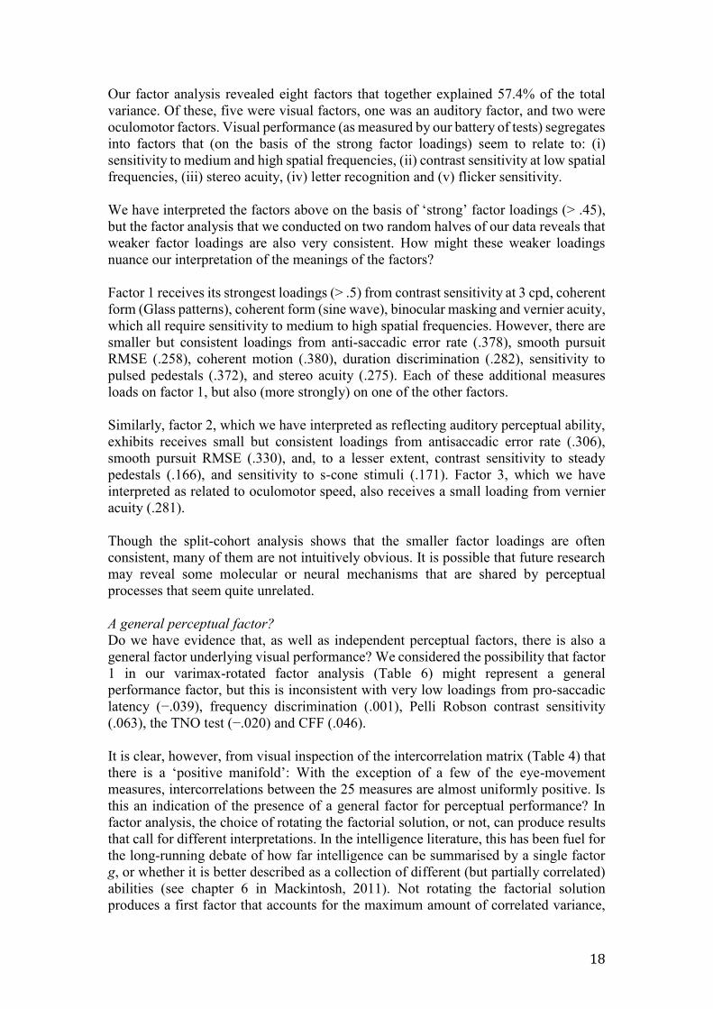
For deciding the number of factors to retain, we applied the criterion that eigenvalues

should be greater than 1. This criterion is widely used but has been criticized (Courtney,

2013). One alternative strategy is to inspect a 'scree plot' – a plot of eigenvalue against

factor number – for a sudden change in the gradient. Figure 1 shows a scree plot for

our data. The clearest “elbow” in the plot is at 3 components, suggesting three factors,

but our results (below) do show interpretable and consistent factors beyond 3. In a third

strategy, some researchers have chosen to retain factors so long as they are

interpretable (e.g. Dobkins et al., 2000; MacLeod & Webster, 1983). When we applied

this strategy to our own results, we found that additional factors with eigenvalues <1

loaded strongly only on single variables and therefore did not contribute usefully to the

results. We therefore retained only factors with eigenvalues >1, which, independently,

we do consider interpretable.

11

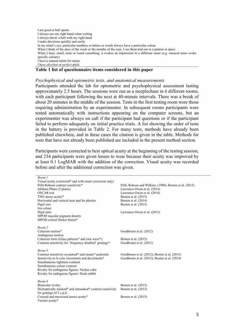
An eight-factor solution accounted for 57.4% of the variance. Eigenvalues and

percentage of variance explained for each factor in both rotated and unrotated solutions

are provided in Table 5, and factor loadings for the rotated solution are presented in

Table 6.

Factor 1 receives strong loadings (> .5) from contrast sensitivity at 3 cpd,

coherent form (Glass patterns), coherent form (sine wave), binocularly masked

contrast sensitivity (also at 3 cpd), and vernier acuity. All of these tests require

sensitivity to medium or high spatial frequencies.

Factor 2 receives strong loadings from the three auditory tasks: duration

discrimination, frequency discrimination and order discrimination. This factor

appears to correspond to auditory perceptual ability.

Factor 3 receives strong loadings from pro-saccadic latency and anti-saccadic

latency. It appears to relate to oculomotor speed.

Factor 4 receives strong loadings from express saccades and latency variability.

This appears to be a factor for oculomotor control.

Factor 5 receives strong loadings from sensitivity to “frequency-doubled”

gratings, sensitivity to pulsed and steady pedestals and sensitivity to s-cone

stimuli. This appears to be a factor relating to contrast sensitivity at low spatial

frequencies.

Factor 6 receives strong loadings from the TNO test and our custom test of

stereo acuity—it relates to stereo acuity.

Factor 7 receives strong loadings from corrected visual acuity and Pelli–Robson

contrast sensitivity. This factor is difficult to interpret. We considered the idea

that it could be a visual acuity factor, but though the letters of the Pelli–Robson

chart have sharp edges, the dominant spatial frequencies are lower than those

that are required for measurements of visual acuity. Since both tests have in

common letters, we provisionally call this factor sensitivity for letter

recognition.

Factor 8 receives loadings from CFF and, to a lesser extent, from sensitivity to

frequency-doubled gratings. This appears to be a factor for flicker sensitivity.

Figure 1 Scree plot.

Unrotated solution Varimax-rotated solution

12

Component Eigenvalue % Variance Eigenvalue % Variance

1 4.99 19.9 2.97 11.89

2 1.95 7.8 1.96 7.86

3 1.46 5.8 1.84 7.35

4 1.40 5.6 1.82 7.29

5 1.3 5.2 1.74 6.98

6 1.18 4.7 1.44 5.74

7 1.06 4.2 1.32 5.28

8 1.01 4.0 1.24 4.97

Table 5 Eigenvalues for and percentage variance explained by each factor, before and

after rotation.

Factor 1 Factor 2 Factor 3 Factor 4 Factor 5 Factor 6 Factor 7 Factor 8

Main sequence .150 .027 .349 −.012 −.366 −.178 .075 .207

Pro-saccadic latency −.039 .112 .817 −.293 .105 .099 .016 −.012

Latency variability .056 .096 .362 .779 .092 .104 .001 −.140

Express saccades .078 .015 −.350 .848 .013 .001 −.010 −.039

Anti-saccadic error rate .378 .306 −.113 .466 .002 .004 .046 .291

Anti-saccadic latency .129 −.089 .669 .105 .045 .011 −.025 .013

Smooth pursuit RMSE .258 .330 .389 .240 .109 .138 .015 .231

Contrast sensitivity (3cpd) .595 .076 .149 .212 .048 −.053 .257 .143

Coherent form (Glass patterns) .748 .089 −.003 −.060 .166 .037 −.078 −.106

Coherent motion .380 .168 .060 .127 .127 .306 .032 .051

Corrected acuity .123 .032 .073 −.030 −.065 .209 .721 .038

Coherent form (sine wave) .721 .074 −.064 −.007 .162 .149 −.031 .024

Duration discrimination .282 .645 .043 .077 .157 .077 −.024 −.081

Frequency discrimination .001 .766 −.039 .023 .081 .081 .052 .081

Frequency doubling .169 −.020 .073 −.027 .601 .121 .016 .453

Order discrimination .154 .743 .049 .046 .055 −.045 .026 .033

Pelli Robson .063 .021 −.073 .032 .236 −.049 .770 −.026

Binocular masking .630 .105 .102 .186 .087 .092 .148 .168

Pulsed pedestals .372 .082 .182 .029 .490 −.188 .089 −.076

Steady pedestals .192 .166 .070 .072 .639 −.094 .154 .230

TNO −.020 −.019 .038 .016 −.011 .776 .187 .095

Vernier acuity .540 .197 .281 .001 .145 .071 .165 .058

Sensitivity to s-cone stimuli .205 .171 .026 .035 .601 .120 .037 −.039

Stereo acuity .275 .103 .035 .034 .045 .703 −.044 −.072

CFF .046 .048 .045 −.062 .090 .018 .003 .824

Table 6. Results of factor analysis on combined data from 1060 participants. Factor

loadings larger than .25 are highlighted in bold.

To test the reliability of the results of the factor analysis, we ran the same analysis but

separately on two, randomly divided and independent, halves of the data, each

containing results from 530 participants. We label the two subsets of participants Group

A and Group B. Both analyses generated eight-factor solutions, and the factor loadings

from both are provided in Table 7.

Factor 1 1 2 2 3 4 4 3 5 5 6 6 7 7 8 8

Group A B A B A B A B A B A B A B A B

Main sequence .13 .09 .00 .08 −.02 −.02 .13 .19 .02 .07 −.12 −.16 .08 −.01 .74 −.55

Pro-saccadic latency −.01 .02 .07 .19 −.37 −.22 .69 .84 .16 .00 .15 −.01 .02 .03 .35 .04

Latency variability .05 .09 .09 .14 .68 .86 .41 .28 .05 −.12 .12 .03 −.01 .07 .21 .05

Express saccades .06 .06 .02 .01 .88 .82 −.24 −.42 −.05 −.02 −.03 .02 −.01 .02 −.08 .02

Anti-saccadic error rate .30 .38 .30 .29 .51 .41 .00 −.21 .10 .32 .04 .09 .02 −.01 −.18 −.25

Anti-saccadic latency .12 .13 −.03 −.15 .08 .13 .74 .71 −.08 .14 −.02 .10 −.07 .02 −.09 −.15

Smooth pursuit RMSE .20 .31 .26 .41 .32 .13 .37 .32 .28 .23 .20 .13 .06 −.08 .09 −.19

Contrast sensitivity (3cpd) .57 .61 .00 .14 .31 .05 .23 .00 .18 .01 −.02 −.04 .23 .25 −.01 −.28

Coherent form (Glass patterns) .78 .73 .14 .04 −.03 .01 −.02 .02 −.01 −.01 −.01 .09 −.02 −.06 .02 .14

Coherent motion .37 .41 .16 .20 .07 .15 .11 −.01 .11 .13 .23 .38 .11 −.07 −.01 .00

Corrected acuity .11 .08 −.03 .08 −.02 −.01 .03 .08 .01 −.01 .33 .15 .63 .74 .09 −.05

Coherent form (sine wave) .77 .67 .09 .05 .02 .07 −.11 −.03 .16 .06 .13 .17 .02 −.04 .03 .12

Duration discrimination .30 .27 .66 .63 .07 .10 .16 .03 .00 −.05 .07 .08 −.04 .04 −.22 .10

Frequency discrimination .00 .02 .76 .76 .06 .01 −.08 −.04 .16 .04 .03 .12 .09 .03 .07 .03

Frequency-doubled gratings .21 .26 −.01 .05 .00 −.02 .07 .11 .75 .61 .07 .04 .11 .00 −.09 .39 Order discrimination .18 .13 .74 .74 .08 .04 .04 .04 .02 .07 −.06 −.02 .00 .05 .02 −.04

Pelli Robson .10 .08 .08 .00 .02 .08 −.06 −.05 .06 .15 −.06 −.06 .83 .74 −.04 .15

13

Binocular masking .62 .62 .11 .09 .29 .04 .17 .00 .21 .07 .10 .12 .06 .29 −.04 −.16

Pulsed pedestals .33 .55 .09 .12 −.04 .06 .36 .15 .17 .15 −.18 −.25 .23 −.03 −.44 .11

Steady pedestals .18 .40 .26 .17 .08 .04 .14 .07 .54 .45 −.06 −.25 .24 .10 −.28 .25 TNO −.02 −.06 −.09 .06 .04 −.02 .05 .04 .11 .09 .78 .77 .17 .14 −.09 −.02

Vernier acuity .53 .56 .16 .23 .05 .01 .31 .24 .17 .02 .10 .04 .18 .13 .06 .07

Sensitivity to s-cone stimuli .30 .30 .22 .21 .10 .00 .12 .08 .32 .14 .11 −.07 .09 .12 −.25 .56

Stereo acuity .31 .28 .12 .12 .02 .05 .01 .07 −.04 −.11 .72 .62 -.05 −.02 .00 .19

CFF .08 −.05 .07 .01 .00 −.09 −.10 .06 .72 .76 .03 .07 -.13 .12 .18 −.17

Table 7. Results of two independent factor analyses on two random halves of the data

(Groups A and B; n = 530 for each). Factor loadings greater than .25 are highlighted in

bold.

For both groups a similar factor structure emerges, one which is also very similar to

that for the full cohort (Table 6). Factors 3 and 4 appear to be in opposite order for the

two groups, and are listed as such in Table 7. The only notable difference between the

solutions for the two groups is for factor 8, which appears to run in opposite directions

for each of the two groups, and which, apart from main sequence, loads differently on

measures of contrast sensitivity for each group. Factor 8 is also different from the factor

8 that emerges from the full cohort: For the two groups factor 8 loads on main sequence,

but for the full cohort, it loads on CFF and sensitivity to frequency-doubled gratings.

In summary, the high consistency of the factor solutions for the two randomly selected

groups gives confidence that the factor solution is stable.

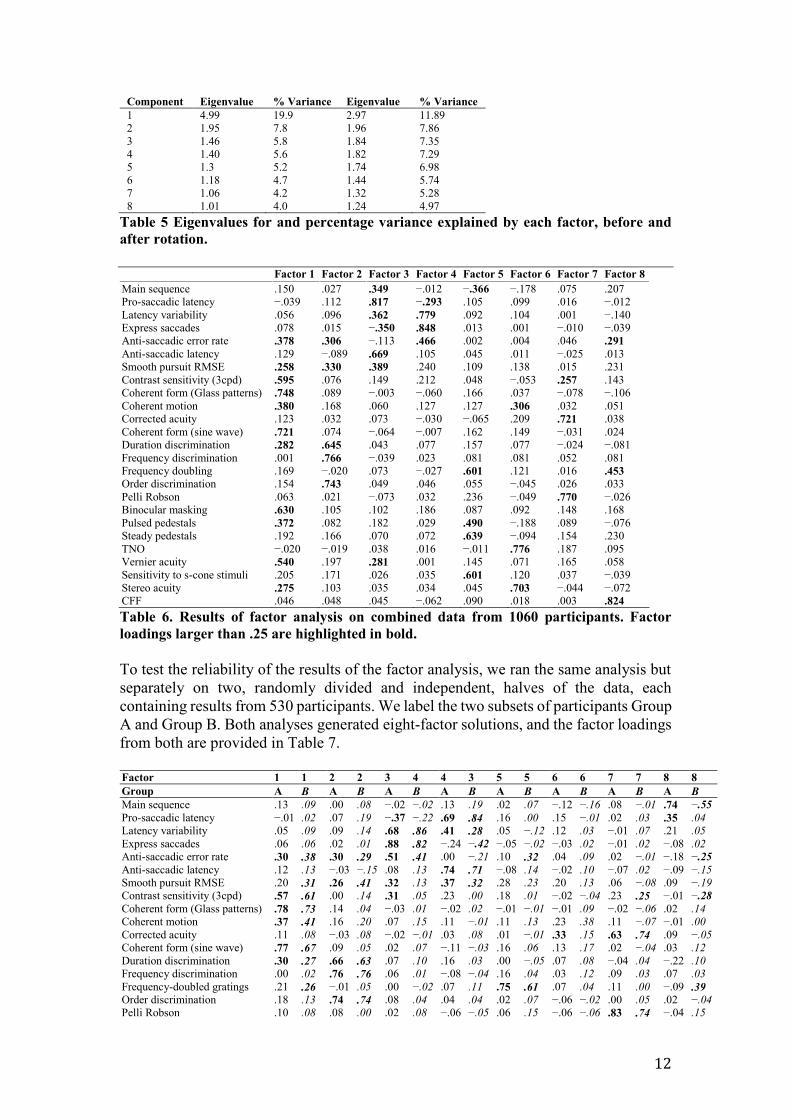
Cluster analysis

We performed a hierarchical cluster analysis (by task) on the results of the same tasks

that were entered into the factor analysis. Since any missing data exclude participants

from the cluster analysis, our sample comprised the 941 participants with complete

data. We used SPSS statistics version 22 (IBM, Armonk, USA) for the analysis.

The resulting dendrogram is shown in Figure 2. Its features tell a similar story to the

factor analysis, as might be expected. Contrast sensitivity at 3 cpd, binocular masking,

vernier acuity, coherent form (Glass patterns) and coherent form (sine wave) cluster:

All require sensitivity to medium or high spatial frequencies. Similarly, the three

auditory tasks form a cluster, as do the two measures of stereo acuity. Another cluster

contains sensitivity to frequency-doubled gratings, sensitivity to steady and pulsed

pedestals, and sensitivity to S-cone stimuli, all measures of contrast sensitivity at low

spatial frequencies. Somewhat unexpected is how the oculomotor measures cluster.

Pro- and anti-saccadic latencies cluster as measures of oculomotor speed, as do express

saccades and latency variability as putative measures of oculomotor control. However,

smooth pursuit RMSE and anti-saccadic error rate cluster with measures of contrast

sensitivity rather than with the other oculomotor measures (on the relationship between

smooth pursuit RMSE and anti-saccadic error rate see Zanelli et al., 2005). This was

not obvious in the results of the factor analysis, but Table 6 shows that both of these

measures load on factors 1 and 2 as well as factor 3 (with other oculomotor measures).

14

Figure 2. Dendrogram showing the results of a hierarchical cluster analysis by variable.

Correlates of the performance factors

In a second-stage analysis, we correlated scores on each of the eight factors that

emerged from the factor analysis with results on the tasks that did not meet our criteria

for inclusion in the factor analysis, and also with the questionnaire items listed in Table

1. Significant correlations are shown in Table 8. We applied a Bonferroni correction

for the 456 correlations.

Some items did not correlate even nominally significantly (i.e., P < .05, uncorrected)

with any factor, and are not included in Table 8. These were the personality factor

‘Intellect/Imagination’, autism quotient, BMI, iris colour and lightness, variance of iris

colour, performance on the Ishihara test for colour vision deficiency (for methods see

Lawrance-Owen et al., 2014), rate of rivalry for the Necker cube, rate of rivalry for the

duck-rabbit figure, and vertical near phoria.

Of the correlations that are significant, most have modest effect sizes, and many are not

unexpected. Agreement with statements “I have a natural talent for music”, “I have

absolute or perfect pitch” and self-reported years spent practicing a musical instrument

correlated significantly with factor 2, which relates to auditory ability. Similarly,

agreement with the statement “I find it difficult to hear and produce sounds in foreign

languages that are different from my native language” correlates negatively with the

same factor. Time spent playing computer games correlates with factor 3, which relates

Main sequence

Contrast sensitivity (3cpd)

Vernier acuity

Binocular masking

Coherent form (sine wave)

Coherent form (Glass patterns)

Frequency doubled gratings

Coherent motion

Smooth pursuit RMSE

Antisaccadic error rate

CFF

Duration discrimination

Pulsed pedestals

Sensitivity to s-cone stimuli

Steady pedestals

Stereo acuity

TNO

Frequency discrimination

Order discrimination

Express saccades

Latency variability

Pelli Robson

Corrected acuity

Antisaccadic latency

Pro saccadic latency

Rescaled distance

15

to oculomotor speed. Factor 7 (on which visual acuity and Pelli-Robson contrast

sensitivity load) correlates with uncorrected visual acuity, usual refraction (strength of

lenses normally worn), and total refraction (strength of usual lenses plus any lenses that

were added following assessment of visual acuity). Our vales for refraction are signed

positive for lenses for hypermetropia and negative for lenses for myopia, though we

note that while 537 participants wore lenses (total refraction) for myopia, only 28 wore

lenses for hypermetropia.

Factor 6, relating to stereo acuity, correlates with far horizontal phoria and uncorrected

visual acuity. These correlations, but with the two measures of stereo acuity

individually, were already reported in Bosten et al. (2015).

Factor 8 (flicker sensitivity) correlates inversely with age and positively with average

pupil size and macular pigment density. All three of these are not unexpected: CFF is

known to reduce with age (e.g. McFarland, Warren, & Karis, 1958), increase with

increasing pupil size following application of pharmacological pupil dilators

(Lawrance, McEwen, Stonier, & Pidgen, 1982), and increase with macular pigment

density (Hammond & Wooten, 2005).

There are two small but significant correlations with personality factors. Factors 1 and

2 correlate inversely with Extraversion, implying that there are inverse relationships

between this personality factor and both contrast sensitivity and auditory ability.

There are two significant correlations with sex: factor 1 (contrast sensitivity) and factor

3 (oculomotor speed), in both cases in the direction of better performance by males.

There is a positive correlation between GCSE score (our surrogate measure for g) and

factor 2 (auditory ability) with a p-value (0.00016) that is marginally greater than the

Bonferroni-corrected alpha (0.00011). Interestingly, there are no significant

correlations between GCSE score and any of the visual or oculomotor factors.

There is a surprising significant correlation between factor 2 (auditory ability) and

susceptibility to simultaneous luminance contrast. There is a positive correlation

between interpupillary distance and factor 3 (oculomotor speed) with a p-value that

falls just above the Bonferroni-corrected alpha (p = 0.00013, α = 0.00011).

Factor 1 Factor 2 Factor 3 Factor 4 Factor 5 Factor 6 Factor 7 Factor 8

Big 5 Agreeableness -.114

Big 5 Contentiousness .069

Big 5 Extraversion -.146 -.140 .074

Big 5 Neuroticism -.095 -.066

Age .065 .076 .092 -.191

Sex -.138 -.165 .087 -.098 -.081

Height .099 .095 -.091 -.071 .108 .101

Weight .103 .113 .101

GCSE points .197 .117

Preferred eye -.102 .067

I always use my right hand when writing .084

I always throw a ball with my right hand .066

I am good at dancing .065 -.076

I am generally good at sport .070

I am good at ball sports -.067 .071

Years spent practicing a musical

instrument .393 .081 .068

I have a natural talent for music .340

16

I have absolute or perfect pitch -.071 .137

I find it difficult to hear and produce

sounds in foreign languages that are

different from my native language -.130

Time spent playing computer games .099 .192

Time spent using a computer -.071

Days per week with heavy drinking .111

I make decisions quickly and easily -.073 .097

I often forget things that have happened in

the past that others remember .065

I have a photographic memory -.081 -.110

I can remember the exact shade of a

colour several days after seeing it -.085 -.070

Combined synaesthesia score .078

Added refraction .120 .088 .111

Total refraction -.085 .122 .186 .081

Uncorrected acuity -.126 -.211 -.526 -.095

Usual refraction -.073 .105 .210

Average pupil size -.095 .115 .192

Interpupillary distance .066 .125 .093

Far horizontal phoria -.068 .128

Far vertical phoria

Near horizontal phoria -.064 .078

OSCAR setting -.096 .065

Macular pigment density .090 -.067 .143

Binocular rivalry rate -.171 -.120 -.098

Standard deviation of percept duration in

binocular rivalry -.081 -.120 -.103

Simultaneous colour contrast .068 .103 .070 .100

Simultaneous luminance contrast -.078 -.174 -.096 .069

Self-rated face ability -.121 .118

Mooney face test .176 .121

Cambridge face memory test .144 .146 -.107

Composite face test .141 .130

Glasgow face matching test .130

Table 8 Significant correlations between factor scores and results on questionnaire

measures, and other visual measures that were not included in the factor analysis. All

nominally significant correlations are shown. Those that survive a Bonferroni correction

for 456 tests are indicated in bold.

Discussion

Intercorrelation matrix

More than half of the intercorrelations between our 25 performance tests listed in Table

4 are significant. However, they are generally modest in size. Figure 3 compares our

observed distribution of Spearman correlation coefficients to a simulated null

distribution, created by conducting 10 000 correlations between randomly sampled

pairs of tests, but randomising the ranks of participants separately for each member of

the pair. The figure shows that the distribution of observed coefficients (solid black

line) is shifted rightward by about .15 compared to the distribution expected under the

null hypothesis (dotted line).

What can we conclude from the size of correlations between our measures? Unless the

test-retest reliabilities are known for individual tests, nothing can be concluded from

the absence or weakness of correlations between tests: an unknown part of the variance

may be due to the first two of the three sources of variance that we identified in the

Introduction: (i) instrumental or measurement error and (ii) intra-individual variability.

Test-retest reliability allows us to estimate these sources of variance, and calculate the

maximum expected correlation between two measures, given the noise that we know

to be present in them. The maximum expected correlation is given by

17

,

where ra and rb are the reliabilities of the two measures, and rt is their true correlation

(i.e. the correlation between the “universe scores”—the means of an infinite number of

measurements).

The dashed line in Figure 3 shows the distribution of maximum expected correlations

given our set of test-retest reliabilities listed in Table 3, in the extreme case that the true

correlation between pairs of variables (rt) is in all cases 1. This distribution has a mean

of r = .68. It is not plausible, of course, that the 25 measures would be perfectly

correlated. With known reliabilities, it is possible to estimate true correlation

coefficients:

,

where ro is the observed correlation (the solid black line in Figure 3). The estimated

distribution of true correlation coefficients between our 25 measures is shown in Figure

3 by the solid grey line. This distribution peaks at r = .32, which is .17 rightward of the

mean of the distribution of observed correlation coefficients.

Figure 3 shows that the distribution of observed correlation coefficients (solid black

line) is much lower than the distribution of maximum expected correlation coefficients

(dashed line): we can conclude that our 25 measures are not perfectly correlated.

Instead, the true correlations between them are likely to range between about 0.15 and

about 0.6 (solid grey line).

Figure 3. Distribution of correlation coefficients. The distribution of correlation

coefficients in Table 4 is indicated by the solid black line. A permuted distribution is

shown by the dotted line: This is the distribution of correlation coefficients that would be

expected by chance. The dashed line shows the maximum observable distribution of

correlation coefficients given the reliabilities of our measures. The solid grey line shows

an estimate of the distribution of true correlation coefficients between our 25 measures,

accounting for their reliabilities. All distributions are scaled so that the areas under the

curves are unity.

Factor analysis

ro = rt rarb

rt =ro

rarb

Spearman's rho-0.5 0 0.5 1

Pro

bab

ility

0

0.1

0.2

0.3

0.4

0.5

0.6

18

Our factor analysis revealed eight factors that together explained 57.4% of the total

variance. Of these, five were visual factors, one was an auditory factor, and two were

oculomotor factors. Visual performance (as measured by our battery of tests) segregates

into factors that (on the basis of the strong factor loadings) seem to relate to: (i)

sensitivity to medium and high spatial frequencies, (ii) contrast sensitivity at low spatial

frequencies, (iii) stereo acuity, (iv) letter recognition and (v) flicker sensitivity.

We have interpreted the factors above on the basis of ‘strong’ factor loadings (> .45),

but the factor analysis that we conducted on two random halves of our data reveals that

weaker factor loadings are also very consistent. How might these weaker loadings

nuance our interpretation of the meanings of the factors?

Factor 1 receives its strongest loadings (> .5) from contrast sensitivity at 3 cpd, coherent

form (Glass patterns), coherent form (sine wave), binocular masking and vernier acuity,

which all require sensitivity to medium to high spatial frequencies. However, there are

smaller but consistent loadings from anti-saccadic error rate (.378), smooth pursuit

RMSE (.258), coherent motion (.380), duration discrimination (.282), sensitivity to

pulsed pedestals (.372), and stereo acuity (.275). Each of these additional measures

loads on factor 1, but also (more strongly) on one of the other factors.

Similarly, factor 2, which we have interpreted as reflecting auditory perceptual ability,

exhibits receives small but consistent loadings from antisaccadic error rate (.306),

smooth pursuit RMSE (.330), and, to a lesser extent, contrast sensitivity to steady

pedestals (.166), and sensitivity to s-cone stimuli (.171). Factor 3, which we have

interpreted as related to oculomotor speed, also receives a small loading from vernier

acuity (.281).

Though the split-cohort analysis shows that the smaller factor loadings are often

consistent, many of them are not intuitively obvious. It is possible that future research

may reveal some molecular or neural mechanisms that are shared by perceptual

processes that seem quite unrelated.

A general perceptual factor?

Do we have evidence that, as well as independent perceptual factors, there is also a

general factor underlying visual performance? We considered the possibility that factor

1 in our varimax-rotated factor analysis (Table 6) might represent a general

performance factor, but this is inconsistent with very low loadings from pro-saccadic

latency (−.039), frequency discrimination (.001), Pelli Robson contrast sensitivity

(.063), the TNO test (−.020) and CFF (.046).

It is clear, however, from visual inspection of the intercorrelation matrix (Table 4) that

there is a ‘positive manifold’: With the exception of a few of the eye-movement

measures, intercorrelations between the 25 measures are almost uniformly positive. Is

this an indication of the presence of a general factor for perceptual performance? In

factor analysis, the choice of rotating the factorial solution, or not, can produce results

that call for different interpretations. In the intelligence literature, this has been fuel for

the long-running debate of how far intelligence can be summarised by a single factor

g, or whether it is better described as a collection of different (but partially correlated)

abilities (see chapter 6 in Mackintosh, 2011). Not rotating the factorial solution

produces a first factor that accounts for the maximum amount of correlated variance,

19

and therefore tends to produce a factor that loads on most of the input variables.

Orthogonally rotating the solution best identifies a set of independent factors that

describe the pattern of correlations—it is this strategy we have pursued here.

If, however, we look at the unrotated results of the principal components analysis for

our 25 measures, the first factor explains 19.9% of the total variance (Table 5),

compared to 11.9% of the variance in the varimax-rotated solution. In the unrotated

solution, all 25 measures load positively on the first factor, with loadings ranging

between .07 and .65 (mean .42, s.d. .17). Considering both rotated and unrotated

solutions, we conclude similarly to the current consensus over factors describing

intelligence (Mackintosh, 2011): There is evidence both for a general factor underlying

perceptual performance, and for independent perceptual abilities. The former is

emphasised in the unrotated solution, and the latter in the rotated solution. We do not

favour the results of either the rotated or the unrotated solution: we believe each provide

a useful contribution to our understanding of the data.

Relationship to previous work

How do our factors compare with those that have similarly aimed to discover factors

underlying visual perception? None of our eight factors match those revealed by the

work of Thurstone (1944), which is unsurprising since the task batteries in the two

studies are very different. Thurstone’s battery emphasised high-level perceptual tasks

and included measures of reaction time, and so it is not surprising that the emerging

factors related to perceptual closure, susceptibility to geometric illusions, reaction time

and perceptual speed. In contrast, our own analysis included sensory threshold

measures of different psychophysical abilities. The precise character of the factors that

emerge from any factor analysis depends on the measures that are put in, and therefore

comparable results are expected from different studies only if comparable task sets are

used.

Our task set had more in common with those of Halpern et al. (1999), Cappe et al.

(2014), and Ward et al. (2016) than that of Thurstone (1944). Halpern et al. provided

loadings only for the first principal component resulting from their PCA. Their

measures of orientation discrimination, wavelength discrimination, contrast sensitivity,

vernier acuity, velocity discrimination and identification of complex form all correlated

with the first principal component, while motion direction discrimination did not. This

first principal component explained somewhat more of the variance (30%) than the first

principal component in our own unrotated principal components analysis (19.9%).

Halpern et al. (1999) did not provide information about subsequent factors, nor a rotated

solution, so it is unclear whether or not their study produced, like ours, evidence for

different factors associated with different perceptual domains.

Cappe et al. (2014) included in their test battery measures of visual acuity, vernier

acuity, backward masking and contrast detection, which are related to our own. In their

study, the first PCA accounted for 34% of the variance – again, a greater percentage

than our own. Although Cappe et al. did not report loadings on each PCA for each of

their tasks, they do report a correlation between vernier acuity and contrast detection.

Our own factor 8, loading on Pelli-Robson contrast detection and visual acuity is a

similar result.

20

Four of the tasks of Ward et al. (2016) were related to our own: their detection of gabors,

contrast sensitivity, detection of Glass patterns, and detection of coherent motion. Our

results are in agreement with Ward et al.’s finding, and also the results of Peterzell and

Teller (Peterzell & Teller, 1996; Peterzell, 2016) that sensitivity to low and high spatial

frequencies load on separate factors. Ward et al. found that sensitivity to Glass patterns

loaded on the same factor as tasks involving high spatial frequencies, while thresholds

for coherent motion loaded on the same factor as tasks involving low spatial

frequencies. Our own results do not show this distinction: thresholds for coherent

motion and sensitivity to Glass patterns both load on factor 1, which is related to other

tasks involving high spatial frequencies.

Cluster analysis

The clusters of tasks revealed by the hierarchical cluster analysis reinforce those

revealed by the factor analysis, as would be expected. One surprising result was the

clustering of anti-saccadic error rate and smooth pursuit RMSE with factor 1

(sensitivity to medium and high spatial frequencies) rather than factors 2 and 3

(oculomotor speed and oculomotor control). However, the detailed factor loadings for

anti-saccadic error rate and smooth pursuit RMSE (Tables 6 and 7) show that they more

distributed over the factors than are the other oculomotor measures (see Zanelli et al.,

2005). Both variables exhibit medium loadings on factors 1, 2 and 8, as well as on factor

4 (factor 3 for Group A in Table 7). It seems to be the case that performance on these

oculomotor measures has more in common with psychophysical performance in other

domains than do saccadic latency and variability.

Correlates of performance factors

Many of the correlations listed in Table 8, between the factors that emerged from the

factor analysis and visual non-performance measures and questionnaire items, are not

surprising. We found significant correlations between factor 2 (auditory ability) and

self-ratings for musical and auditory abilities. It is interesting that time spent playing

computer games correlates with factor 3 (oculomotor speed): Future work will be

needed to disentangle the causal direction.

It is also interesting that GCSE score (our surrogate measure of g) shares variance with

with factor 2 (auditory perceptual ability), but not with any of the factors relating to

visual perceptual ability. Since foreign language exams are taken by most GCSE

students, a portion of the variance in GCSE score (perhaps about 10%) may reflect

foreign language ability, which is likely to be related to auditory ability. However, it is

unlikely that this fully accounts for the correlation: Our result is compatible with earlier

reports of modest but significant correlations between auditory abilities and general

cognitive ability (e.g. Burt, 1909; Carey, 1915; Kidd, Watson, & Gygi, 2007).

The shared variance between interpupillary distance and factor 3 (oculomotor speed)

could be largely explained by sex, which also correlates with factor 3. When sex is

included as a covariate in a partial correlation, rho falls to .06 (P = .06). It is, of course,

also possible that the dependencies go in a different direction: that the correlation

between sex and factor 3 is mediated by interpupillary distance.

Some relationships are curious by their absence. None of our factors is strongly

correlated with Autism-spectrum Quotient, despite the large literature relating

perceptual measures to autism (Simmons et al., 2009). It is also interesting that none of

21

the factors relates to lightness of the iris, which is known to affect the level of stray

light in the retina (van den Berg, Ijspeert, & de Waard, 1991). Though it is a priori very

plausible that the personality variable Conscientiousness would contribute to

psychophysical performance, we have found that no performance factor correlates

significantly with it, and neither does it correlate with factor 1 of the unrotated factorial

solution, our putative general factor for perceptual performance.

Conclusions

Our factor analysis of perceptual performance has revealed evidence both for a general

factor underlying perceptual ability (accounting, in the unrotated solution, for 19.9% of

the total variance) and for independent factors that account for performance on

particular groups of measures. The independent factors we identified (though they will

depend on the component measures included in the analysis) relate to (1) sensitivity to

medium and high spatial frequencies, (2) auditory perceptual ability (3) oculomotor

speed, (4) oculomotor control, (5) contrast sensitivity at low spatial frequencies, (6)

stereo acuity, (7) letter recognition, and (8) flicker sensitivity.

Acknowledgements

This work was supported by the Gatsby Charitable Foundation (GAT2903). J.B. was

supported by a fellowship from Gonville and Caius College. The authors are grateful

to Horace Barlow, Roger Freedman, Graeme Mitchison and Richard Durbin for their

role in the initiation of the PERGENIC project. We thank David Peterzell and Michael

Herzog for their valuable comments as reviewers.

References

Aspinall, P. (1974). Some methodological problems in testing visual function. In G.

Verriest (Ed.), Modern problems in ophthalmology: colour vision dediciencies II

(pp. 1–7). Basel: S. Karger.

Bargary, G., Bosten, J., Goodbourn, P., Lawrance-Owen, A., Hogg, R., & Mollon, J.

(n.d.). Individual differences in human eye movements: an oculomotor signature?

In Press at Vision Research.

Baron-Cohen, S., Wheelwright, S., Skinner, R., Martin, J., & Clubley, E. (2001). The

autism-spectrum quotient (AQ): evidence from Asperger syndrome/high-

functioning autism, males and females, scientists and mathematicians. Journal of

Autism and Developmental Disorders, 31(1), 5–17.

Beard, R. M. (1965). The structure of perception: a factorial study. The British Journal

of Educational Psychology, 35, 210–222.

Bosten, J. M., Bargary, G., Goodbourn, P. T., Hogg, R. E., Lawrance-Owen, A. J., &

Mollon, J. D. (2014). Individual differences provide psychophysical evidence for

separate on- and off-pathways deriving from short-wave cones. Journal of the

Optical Society of America. A, Optics, Image Science, and Vision, 31(4), A47-54.

Bosten, J. M., Goodbourn, P. T., Lawrance-Owen, A. J., Bargary, G., Hogg, R. E., &

Mollon, J. D. (2015). A population study of binocular function. Vision Research,

110(Part A), 34–50. http://doi.org/10.1016/j.visres.2015.02.017

Bosten, J. M., Hogg, R. E., Bargary, G., Goodbourn, P. T., Lawrance-Owen, A. J., &

Mollon, J. D. (2014). Suggestive association with ocular phoria at chromosome

6p22. Investigative Ophthalmology & Visual Science, 55(1), 345–52.

http://doi.org/10.1167/iovs.13-12879

Browne, M. (2001). An overview of analytic rotation in exploratory factor analysis.

Multivariate Behavioral Research, 36, 111–150.

22

Burt, C. (1909). Experimental tests of general intelligence. British Journal of

Psychology, 3, 94–177.

Cappe, C., Clarke, A., Mohr, C., & Herzog, M. H. (2014). Is there a common factor for

vision? Journal of Vision, 14(2014), 1–11. http://doi.org/10.1167/14.8.4.doi

Carey, N. (1915). Factors in the Mental Processes of School Children. II. On the Nature

of Specific Mental Factors. British Journal of Psychology, 8, 70–92.

Courtney, M. G. R. (2013). Determining the number of factors to retain in EFA: Using

the SPSS R-Menu v2.0 to make more judicious estimations. Practical Assessment,

Research & Evaluation, 18(8), 1–14.

Deary, I. J., Strand, S., Smith, P., & Fernandes, C. (2007). Intelligence and educational

achievement. Intelligence, 35(1), 13–21.

http://doi.org/10.1016/j.intell.2006.02.001

Diener, D. (1986). A factor analytic study of hue discrimination. Perception and

Psychophysics, 38(5), 443–449.

Dobkins, K. R., Gunther, K. L., & Peterzell, D. H. (2000). What covariance

mechanisms underlie green/red equiluminance, luminance contrast sensitivity and

chromatic (green/red) contrast sensitivity? Vision Research, 40(6), 613–28.

Donnellan, M., Oswalk, F., Baird, B., & Lucas, R. (2006). The mini-IPIP scales: tiny-

yet-effective measures of the Big Five factors of personality. Psychological

Assessment, 18(2), 192–203.

Duncan, R. O., & Boynton, G. M. (2003). Cortical magnification within human primary

visual cortex correlates with acuity thresholds. Neuron, 38(4), 659–671.

http://doi.org/10.1016/S0896-6273(03)00265-4

Goodbourn, P. T., Bosten, J. M., Bargary, G., Hogg, R. E., Lawrance-Owen, a J., &

Mollon, J. D. (2014). Variants in the 1q21 risk region are associated with a visual

endophenotype of autism and schizophrenia. Genes, Brain, and Behavior, 13(2),

144–51. http://doi.org/10.1111/gbb.12096

Goodbourn, P. T., Bosten, J. M., Hogg, R. E., Bargary, G., Lawrance-Owen, A. J., &

Mollon, J. D. (2012). Do different “magnocellular tasks” probe the same neural

substrate? Proceedings of the Royal Society B: Biological Sciences, 279, 4263–

4271. http://doi.org/10.1098/rspb.2012.1430

Gunther, K., & Dobkins, K. (2003). Independence of mechanisms tuned along cardinal

and non-cardinal axes of color space: evidence from factor analysis. Vision

Research, 43(6), 683–696. http://doi.org/10.1016/S0042-6989(02)00689-2

Halpern, S. D., Andrews, T. J., & Purves, D. (1999). Interindividual variation in human

visual performance. Journal of Cognitive Neuroscience, 11(5), 521–34.

Hammond, B. R., & Wooten, B. R. (2005). CFF thresholds: Relation to macular

pigment optical density. Ophthalmic and Physiological Optics, 25(4), 315–319.

http://doi.org/10.1111/j.1475-1313.2005.00271.x

Jones, F. N. (1948). A factor analysis of visibility data. The American Journal of

Psychology, 61(3), 361–369.

Jones, F. N., & Jones, M. (1950). A second factor analysis of visibility data. The

American Journal of Psychology, 63(2), 206–213.

Kanai, R., Bahrami, B., & Rees, G. (2010). Human parietal cortex structure predicts

individual differences in perceptual rivalry. Current Biology : CB, 20(18), 1626–

30. http://doi.org/10.1016/j.cub.2010.07.027

Kanai, R., & Rees, G. (2011). The structural basis of inter-individual differences in

human behaviour and cognition. Nature Reviews Neuroscience, 12(April), 231–

242. http://doi.org/10.1038/nrn3000

Karlin, J. (1942). A factorial study of auditory function. Psychometrika, 7(4), 251–279.

23

Keehn, J. D. (1956). A Modified Interpretation of Thurstone’s Flexibility of Closure

Factor. The Journal of Social Psychology, 44(2), 215–222.

http://doi.org/10.1080/00224545.1956.9921923

Kidd, G. R., Watson, C. S., & Gygi, B. (2007). Individual differences in auditory

abilities. The Journal of the Acoustical Society of America, 122(1), 418–435.

http://doi.org/10.1121/1.4743842

Kihlstrom, J. (2012). Joseph Jastrow and His Duck -- Or Is it a Rabbit? Retrieved from

http://ist-socrates.berkeley.edu/~kihlstrm/JastrowDuck.htm

King-Smith, P. E., Grigsby, S. S., Vingrys, A. J., Benes, S. C., & Supowit, A. (1994).

Efficient and unbiased modifications of the QUEST threshold method: theory,

simulations, experimental evaluation and practical implementation. Vision

Research, 34(7), 885–912.

König, A., & Dieterici, C. (1892). Die Grundempfindungen in normalen und anomalen

Farbensystemen und ihre Intensitätsverteilung im Spektrum. Zeitschrift Für

Psychologie Und Physiologie Der Sinnesorgane, 4, 241–347.

Lawrance-Owen, A. J. (2012). Human variation in colour perception and in

anthropomorphic characteristics. University of Cambridge.

Lawrance-Owen, A. J., Bargary, G., Bosten, J. M., Goodbourn, P. T., Hogg, R. E., &

Mollon, J. D. (2013). Genetic association suggests that SMOC1 mediates between

prenatal sex hormones and digit ratio. Human Genetics, 132(4), 415–421.

http://doi.org/10.1007/s00439-012-1259-y

Lawrance-Owen, A. J., Bosten, J. M., Hogg, R. E., Bargary, G., Goodbourn, P. T., &

Mollon, J. D. (2014). Counterphase modulation flicker photometry: phenotypic

and genotypic associations. Journal of the Optical Society of America. A, 31(4),

A226-31.

Lawrance, J., McEwen, J., Stonier, P., & Pidgen, A. (1982). Fusion, Pupil size and

critical flicker. Drug Development Research, 1, 67–75.

Mackintosh, N. J. (2011). IQ and human intelligence. Oxford: Oxford University Press.

MacLeod, D. I., & Boynton, R. M. (1979). Chromaticity diagram showing cone

excitation by stimuli of equal luminance. Journal of the Optical Society of

America, 69(8), 1183–6.

MacLeod, D., & Webster, M. A. (1983). Factors influencing the color matches of

normal observers. In J. Mollon & L. T. Sharpe (Eds.), Color Vision (pp. 81–92).

London: Academic Press.

McFarland, R. A., Warren, A. B., & Karis, C. (1958). Alterations in critical flicker

frequency as a function of age and light:dark ratio. Journal of Experimental

Psychology, 56(6), 529–538. http://doi.org/10.1037/h0049128

Mooney, C. M. (1954). A factorial study of closure. Can J Psychol, 8(2), 51–60.

http://doi.org/10.1037/h0083599

Mulaik, S. (2009). Foundations of factor analysis (second edi). Boca Raton: CRC

Press.

Murray, I., & Carden, D. (2008, January). The MPod - a new instrument for measuring

macular pigment. Optician, 32–34.

Nathans, J., Piantanida, T. P., Eddy, R. L., Shows, T. B., & Hogness, D. S. (1986).

Molecular genetics of inherited variation in human color vision. Science (New

York, N.Y.), 232(4747), 203–10.

Necker, L. (1832). LXI. Observations on some remarkable optical phænomena seen in

Switzerland; and on an optical phænomenon which occurs on viewing a figure of

a crystal or geometrical solid. Philosophical Magazine Series 3, 1(5), 329–337.

Pelli, D., Robson, J., & Wilkins, A. (1988). The design of a new letter chart for

24

measuring contrast sensitivity. Clinican Vision Sciences, 2(3), 187–199.

Peterzell, D. H. (2016). Discovering sensory processes using individual differences: A

review and factor analytic manifesto. Human Vision and Electronic Imaging, 112,

1–11. http://doi.org/10.2352/ISSN.2470-1173.2016.16HVEI-112

Peterzell, D. H., & Teller, D. Y. (1996). Individual differences in contrast sensitivity

functions: the lowest spatial frequency channels. Vision Research, 36(19), 3077–

85.

Peterzell, D. H., & Teller, D. Y. (2000). Spatial frequency tuned covariance channels

for red-green and luminance- modulated gratings: psychophysical data from

human adults. Vision Research, 40(4), 417–430. http://doi.org/10.1016/S0042-

6989(99)00188-1

Pickford, R. (1962). A brief review of some factorial studies of colour vision. Die

Farbe, Nr. 1/6, 59–68.

Schwarzkopf, D. S., Song, C., & Rees, G. (2011). The surface area of human V1

predicts the subjective experience of object size. Nature Neuroscience, 14(1), 28–

30. http://doi.org/10.1038/nn.2706

Simmons, D. R., Robertson, A. E., McKay, L. S., Toal, E., McAleer, P., & Pollick, F.

E. (2009). Vision in autism spectrum disorders. Vision Research, 49(22), 2705–

2739. http://doi.org/10.1016/j.visres.2009.08.005

Song, C., Schwarzkopf, D. S., & Rees, G. (2013). Variability in visual cortex size

reflects tradeoff between local orientation sensitivity and global orientation

modulation. Nature Communications, 4, 2201.

http://doi.org/10.1038/ncomms3201

Spearman, C. (1904a). “General Intelligence,” Objectively Determined and Measured.

The American Journal of Psychology, 15(2), 201–292.

http://doi.org/10.1525/rac.2012.22.2.265.This

Spearman, C. (1904b). The proof and measurement of association between two things.

The American Journal of Psychology, 15(1), 72–101.

Spearman, C. (1927). The abilities of man. New York: The MacMillan Company.

http://doi.org/10.1126/science.68.1750.38-a

Thurstone, L. L. (1931). Multiple factor analysis. Psychological Review, 38(5), 406–

427.

Thurstone, L. L. (1944). A Factorial Study of Perception. Psychometric Monographs,

4(1), 111–148.

Thurstone, L. L. (1950). Some Primary Abilities in Visual Thinking. Proceedings of

the American Philosophical Society, 94(6), 517–521.

van den Berg, T. J. T. P., Ijspeert, J. K., & de Waard, P. W. T. (1991). Dependence

pigmentation of intraocular straylight on and light transmission through the ccular

wall. Vision Research, 31(7/8), 1361–1367.

Van Der Veen, R. L. P., Berendschot, T. T. J. M., Hendrikse, F., Carden, D., Makridaki,

M., & Murray, I. J. (2009). A new desktop instrument for measuring macular

pigment optical density based on a novel technique for setting flicker thresholds.

Ophthalmic and Physiological Optics, 29(2), 127–137.

http://doi.org/10.1111/j.1475-1313.2008.00618.x

Verhallen, R. J., Bosten, J. M., Goodbourn, P. T., Bargary, G., Lawrance-owen, A. J.,

& Mollon, J. D. (2014). An online version of the Mooney Face Test: phenotypic

and genetic associations. Neuropsychologia, 63, 19–25.

Verhallen, R. J., Bosten, J. M., Goodbourn, P. T., Lawrance-Owen, A. J., Bargary, G.,

& Mollon, J. D. (n.d.). General and specific factors in the processing of faces. In

Press at Vision Research.

25

Ward, J., Rothen, N., Chang, A., & Kanai, R. (2016). The structure of inter-individual

differences in visual ability: Evidence from the general population and

synaesthesia. Vision Research. http://doi.org/10.1016/j.visres.2016.06.009

Wasserstein, J., Barr, W. B., Zappulla, R., & Rock, D. (2004). Facial closure:

Interrelationship with facial discrimination, other closure tests, and subjective

contour illusions. Neuropsychologia, 42(2), 158–163.

http://doi.org/10.1016/j.neuropsychologia.2003.07.003

Watson, A. B., & Pelli, D. G. (1983). QUEST: a Bayesian adaptive psychometric

method. Perception & Psychophysics, 33(2), 113–20.

Wilmer, J. B. (2008). How to use individual differences to isolate functional

organization, biology, and utility of visual functions; with illustrative proposals

for stereopsis. Spatial Vision, 21(6), 561–79.

http://doi.org/10.1163/156856808786451408

Winderickx, J., Lindsey, D. T., Sanocki, E., Teller, D. Y., Motulsky, A. G., & Deeb, S.

S. (1992). Polymorphism in red photopigment underlies variation in colour

matching. Nature.

Zanelli, J., Simon, H., Rabe-Hesketh, S., Walshe, M., McDonald, C., Murray, R. M., &

MacCabe, J. H. (2005). Eye tracking in schizophrenia: Does the antisaccade task

measure anything that the smooth pursuit task does not? Psychiatry Research,

136(2–3), 181–188. http://doi.org/10.1016/j.psychres.2004.12.008

Zychaluk, K., & Foster, D. H. (2009). Model-free estimation of the psychometric

function. Attention, Perception & Psychophysics, 71(6), 1414–25.

http://doi.org/10.3758/APP.71.6.1414