An Explicit Multi-Model Compressible Flow

Formulation Based on the Full Potential

Equation and the Euler Equations on 3D

Unstructured Meshes∗

Xiao-Chuan Cai † Marius Paraschivoiu ‡ Marcus Sarkis §

1 Introduction

The development of a multi-model formulation to simulate three dimensionalcompressible flows on parallel computers is presented. The goal is to reduce theoverall time and memory required to simulate the flow by using locally selectedcheaper and more computational efficient physical models without sacrificing theglobal fidelity of the simulation. Our approach involves splitting the computa-tional domain into different fluid flow regions and using the full potential modelinstead of the Euler or Navier-Stokes equations in regions where this approxi-mation is valid. We show numerically that solving the full potential equationin regions of irrotational flow is not only more efficient but also improves theaccuracy; avoiding any numerical generation of entropy. The main considera-tions addressed in this paper are the full potential and the Euler coupling andthe discretization of the interface conditions between these domains. We usea fully unstructured finite volume discretization for both the full potential andthe Euler equations, and the interface condition is derived by imposing the dis-crete conservation laws in the control volumes shared by both flow regions. 3Dtransonic flow simulations around a NACA0012 airfoil are investigated.

Numerical simulations of fluid flow have sufficiently matured to be consideredaccurate for engineering design and analysis. However, for large scale simula-tions, the response time remains too large for the software to be used as aninteractive tool even on the lastest supercomputers. While parallel computingreduces computation time proportionally to additional computational resource,

∗The work was supported in part by the NSF grants ASC-9457534, ECS-9527169, andECS-9725504.

†Dept. of Comp. Sci., Univ. of Colorado, Boulder, CO 80309. cai@cs.colorado.edu‡Dept. of Comp. Sci., Univ. of Colorado, Boulder, CO 80309. marius@cs.colorado.edu§Math. Sci. Dept., Worcester Poly. Inst., Worcester, MA 01609. msarkis@wpi.edu

1

new algorithms should be constructed to perform faster on new and existingresources. In this paper we describe the initial steps for the development of amulti-model formulation to decrease the computation time of three dimensionalcompressible flow simulations on unstructured grids.

Compressible fluid flow simulations needed for aerodynamic applications canbe modeled with different degree of sophistication. The simplest model is thefull potential equation which assumes inviscid, irrotational and isentropic flows.This equation is a single second-order nonlinear differential equation that isinexpensive with respect to the execution time and the memory requirement.Validity of the full potential equation is, however, restricted. The isentropicassumption of the potential flow model leads to inaccurate physics for transonicflows with strong shocks. The next level of approximation is the Euler equationswhich describe the complete behavior of inviscid compressible flows. The Eulerequations are a coupled system of five nonlinear differential equations of firstorder. Note that this set of equations involves five field variables. Finally, theNavier-Stokes equations include the viscous effects needed for accurate model-ing of the boundary layer. However, these equations are not only more timeconsuming to solve but also require an associated mesh that is stretched andvery fine in viscous regions. Nevertheless, for complex flows with separation ofthe boundary layer, the Navier-Stokes equations are mandatory to provide anaccurate simulation. Furthermore, for high Reynolds number flows, turbulenceappears and needs to be modeled.

When considering transonic flows over a wing, three regions can be iden-tified: the boundary layer, the region around the shock, and the farfield. Amulti–model formulation can be used to combine the strength of each modeldescribed above. Indeed, a multi-model formulation will take advantage of thequick computational time associated with solving the full potential equationwhile capturing all the important features of the flow such as boundary lay-ers and shocks using the Navier-Stokes equations and/or the Euler equations,respectively. Furthermore, we can benefit from the extensive experience of nu-merical methods and software developed over the years to solve these equationsseparately.

Numerical techniques for the solution of the full potential equation and theEuler/Navier-Stokes equations were developed respectively in the 1970s and inthe 1980s [2, 10, 13, 15, 18]. Indeed, compressible flow around entire aircraftshave been simulated. For example, the full potential equation has been solvedfor a 747-200 transport configuration with wing, body, struts, and nacelles [23].For the Euler model, calculations over a complete aircraft have been performedas early as in 1986 [15]. On the other hand, accurate viscous simulations athigh Reynolds number over such complex geometries require enormous compu-tational resources. Approximate solutions, i.e., with less than adequate numberof mesh points, have been performed. A Navier-Stokes prediction for the F–18wing and fuselage is presented in [6]. A discussion of the drastic difference incomputational cost related to the choice of models can be found in [14].

2

However only recently have there been interests to couple these solvers toreduce the computational cost, to reduce the memory requirement and to im-prove the accuracy of the solution. Certainly, boundary layer coupling or thinlayer Navier-Stokes coupling have been widely used but such approaches do notquite include all the physics we intend to incorporate [22]. For some mathemati-cal description of coupling heterogeneous models for compressible flows we referthe readers to [19]. For three dimensional flows, it is shown in [1, 20] that thecomputation cost can be reduced by a factor of two for a Navier-Stokes/full po-tential coupling. Their formulation is based on a structured grid discretizationwhere the full potential equation is solved using a finite difference method andthe Navier-Stokes equations are solved either with a finite difference or a finitevolume discretization. The saving is justified by the fact that two third to onehalf of the cells are outside the Navier-Stokes region. In general, the cost of thefull potential solver can be considered negligible compared to the Navier-Stokessolver. Note that each region is solved alternatively, similar to a subdomainiterative method.

Our formulation differs from [1, 20] by providing a general finite volumeapproach and therefore ensure that the mass will also remain conserved at thediscrete level. This approach also has the advantage of being readily extended toa coupled implicit scheme. While in [1, 20] each region is solved separately, weare expecting to improve convergence by solving the coupled system simultane-ously. In addition, an unstructured discretization of the computational domainprovides more flexibility to mesh complex geometry and for adaptive controlof the numerical error. Lastly, a parallel version is implemented to obtain thereasonable execution time.

In this paper we address the initial step of this research. We first investigatethe coupling between the full potential equation and the Euler equations. Inaddition to the computational savings, solving the full potential equation inthe vicinity of the stagnation point is more accurate by avoiding the numericalentropy generated by Euler solvers at low Mach numbers. Furthermore, the fullpotential solver is less sensitive to the quality of the elements. Both the Eulerand the Navier-Stokes solvers calculate convective fluxes through edges. Whenthe surface of the control volume is different from the perpendicular surfaceof the edges, a numerical error is created. This error does not appear in thefull potential discretization because fluxes are constants in each element. Asmentioned above, a finite volume formulation is adopted to adequately interfacethese different solvers. An explicit approach is first considered to validate thespatial discretization but also as a precursor to the implicit implementation [17].

For simplicity, we address steady flows. For unsteady flows, it is required tohave the temporal derivative of the density which is difficult to include in ourexplicit scheme because this derivation involves potential values of the neigh-boring control volumes. However, in an implicit solver such discretization canbe easily included. As already mentioned, to obtain the most accurate flow sim-ulation, the full Navier-Stokes equations need to be included in our multi-model

3

formulation.A more urgent objective, however, is to address some algorithmic exten-

sions. First, we intend to develop an implicit scheme which is essential for largescale simulations [17]. The convergence rates reported with implicit schemes aremuch faster, in particular when using methods such as the overlapping Schwarzpreconditioned GMRES methods [3]. In our formulation, the Jacobian matrixused in the implicit approach will include the spatial discretization of two ormore equations. It is expected that such system is not positive definite and thusit is not clear how it can be solved efficiently or which preconditioner shouldperform well. Second, we plan to develop a procedure to automatically posi-tion the interface between the different computational domains based on theexisting field variables (i.e., dynamic zonal configuration). Third, we need toconsider load balancing for parallel computations, in particular when dynamiczonal configuration procedures will be used. Recall that different partial differ-ential equations are solved in different regions but each equation does not requirethe same number of operations. One palliative is to decompose each region intosubregions equal to the number of processors. By using such an approach, wecan allocated one subregion of each type to each processor. Finally, we expectthat the outcome of this research will lead to a dramatic reduction in compu-tational time and memory resources to allow faster simulation of compressibleflows including turbulent viscous effect, in particular for external aerodynamicsapplications.

In this paper we focus on the description of the two-model formulation.Section 2 describes the explicit full potential solver and the Euler solver withmore emphasis on the full potential solver. In Section 3, we briefly introducethe coupled solver and compare two types of interface conditions with overlapand without overlap. To demonstrate the feasibility of our approach we solve atransonic flow over a NACA0012 airfoil at zero angle of attack which is analyzedin Section 4. We conclude with remarks and extensions in Section 4.

2 Simulation of compressible flows

Our interest lies in the numerical simulation of three dimensional compress-ible invisid flows. We assume that there is no external force or heat transfer.As described above, these flows can be modeled with the Euler equations orwith the full potential equation for the particular case when the irrotationaland isentropic flows assumption is satisfied. For simplicity of presentation, allthe descriptions given in the paper are based on the first order finite volumediscretization, and the extension to the 2nd order discretization is easy. Allthe numerical results presented in Section 4 are for, however, the 2nd orderdiscretization.

4

2.1 The governing equations

Let Ω ⊂ 3 be the computational flow domain and Γ its boundary. The con-servative form of the Euler equations is given by

∂U

∂t+ ∇ · F (U) = 0. (1)

Here U contains the conservative variables, i.e., U = (ρ, ρu, ρv, ρw, ρE)T . Theexplicit definitions of F () can be found on page 87 of [11]. When the flowis irrotational, there exists a potential variable Φ satisfying the full potentialequation

∂ρ(Φ)∂t

+ ∇ · G(Φ) = 0, (2)

where G(Φ) = ρ∇Φ and∇Φ = (u, v, w)T . (3)

In the rest of the paper, we shall refer to U as the Euler variable, which is avector, and Φ as the full potential variable, which is a scalar.

By appealing to the isentropic flow assumption we can write the density ρas a nonlinear function of the potential, such as

ρ(Φ) = ρ∞

(1 +

γ − 12

M2∞

(1 − ||∇Φ||22

q2∞

))1/(γ−1)

. (4)

There are two types of boundaries that bound the computational domainfor external flows past bodies or obstacles: the farfield boundary and the solidwall boundary. On the solid wall boundary, Γw, the normal velocity, vn, iszero, since no mass crosses the boundary. On the farfield, Γ∞, we impose anuniform free-stream state defined by the following parameters: the density, ρ∞,the velocity vector, v∞, the pressure, p∞, and the Mach number M∞. Theseconditions are given by

vn = 0, on Γw (5)

and

ρ∞ = 1, v∞ =

⎛⎝ cos(α) × cos(θ)

sin(θ)sin(α) × cos(θ)

⎞⎠ , p∞ =

1γM2

∞on Γ∞, (6)

where α and θ are the angles of the flow direction (the angle of attack and theyaw angle, respectively).

2.2 The Euler solver

To solve the Euler equations, we take advantage of an existing code based onan unstructured finite volume discretization of the convective fluxes [7, 8]. The

5

computational flow domain is divided into tetrahedrons to provide maximumflexibility for tessellating complex geometries. Euler variables are located at thevertices of the elements. This code uses a second order flux discretization basedon the MUSCL (Monotonic Upwind Scheme for Conservative Laws) scheme [16].A classical forward Euler method for time integration with a local time step sizeis chosen. Recall that we are only interested in solving the steady state and asimple time integration scheme offers more flexibility to be coupled with the fullpotential solver. The local time step size ∆tnτc

iis defined for each control volume

τci (with characteristic size ‖hc

i‖) by

∆tnτci

= ‖hci‖

CFLCn

τci

+ ‖Unτc

i‖2

, (7)

where CFL is a preselected positive number, Cnτc

iis the sound speed and Un

τci

isthe velocity vector at the nth time step.

The spatial discretization of the boundary condition, (5)-(6), is obtainedusing a non-reflecting version of the flux–splitting scheme [7].

2.3 The full potential solver

A new finite volume full potential solver is developed to adequately interfacewith the existing Euler solver. Therefore, the same control volume is used andonly the flux calculations are different. We describe now the spatial discretiza-tion of the mass flux required in this scheme.

2.3.1 The spatial discretization

The integral form of the full potential equation for the discrete volume τci is

simply ∫τc

i

∇ · G(Φ)dA = 0. (8)

Note that the sum of all τci covers the whole domain Ω, i.e., Ω =

⋃τci . By

analogy to the discretization of the Euler equations, the discretization hereis accomplished by dividing the domain into tetrahedron elements, τh

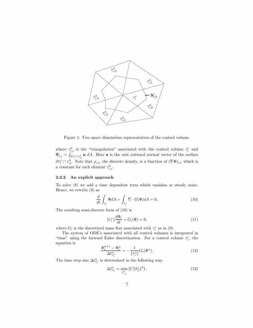
i,j . Thepotential variable is stored at the vertices. This choice is illustrated in Fig. 1 fortwo space dimensions. By using this discretization, the space of the potentialsolution is taken to be piecewise linear continuous functions in each elementdetermined from the vertices values, Φi.

For the control volume τci associated with the dual mesh, we can write the

discrete form of (8) as∫

τci

∇(ρ∇Φ)dA =∫

∂τci

ρ∇Φ · n dS =∑τh

i,j

ρi,j(∇Φ)i,j · Sci,j , (9)

6

τhi,1

τci

τhi,2

τhi,3

τhi,4

τhi,5

τhi,6

Sci,6

Figure 1: Two space dimensions representation of the control volume.

where τhi,j is the “triangulation” associated with the control volume τc

i andSc

i,j =∫

∂τci∩τh

ijn dA. Here n is the unit outward normal vector of the surface

∂τci ∩ τh

ij . Note that ρi,j , the discrete density, is a function of (∇Φ)i,j which isa constant for each element τh

i,j .

2.3.2 An explicit approach

To solve (8) we add a time dependent term which vanishes at steady state.Hence, we rewrite (8) as

d

dt

∫τc

i

ΦdA +∫

τci

∇ · G(Φ)dA = 0. (10)

The resulting semi-discrete form of (10) is

‖τci ‖

dΦi

dt+ Gi(Φ) = 0, (11)

where Gi is the discretized mass flux associated with τci as in (9).

The system of ODE’s associated with all control volumes is integrated in“time” using the forward Euler discretization. For a control volume τc

i , theequation is

Φn+1i − Φn

i

∆tnτci

= − 1‖τc

i ‖Gi(Φn). (12)

The time step size ∆tnτci

is determined in the following way,

∆tnτci

= minτh

i,j

(C‖hc

j‖2), (13)

7

where ‖hcj‖ is the characteristic length of element τh

i,j and C is a global con-stant. Because of the nonlinearity of this equation, it is difficult to determineC analytically. However, based on our numerical experiments, C equal to 0.4 isa good approximation.

2.3.3 The density upwinding scheme

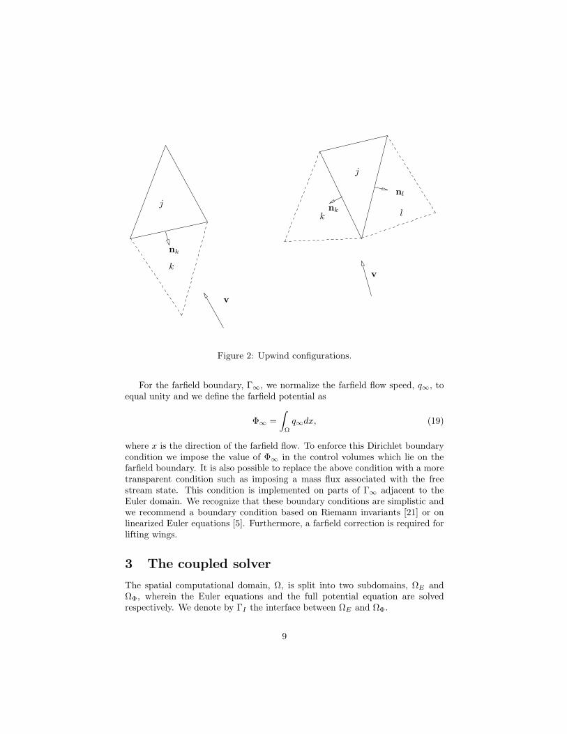
For transonic flows, upwinding is required; therefore, the density is modifiedto add artificial compressibility. The upwinding is introduced prior to the fluxcalculation after which the same subsonic procedure is used. For simplicity, wedescribe our upwinding method for two space dimensions. Following [12, 23],we write

ρ = ρ − µv · ∇−ρ, (14)

where v is the normalized element velocity and ∇−ρ is an upwind difference.In two space dimensions there are two cases to consider. Either the mass fluxenter on one side (Fig. 2 a) or the mass flux enter through two sides (Fig. 2 b).It follows that the density for each case becomes

ρj = ρj + µv · nk(ρj − ρk) (15)ρj = ρj + µv · nk(ρj − ρk) + µv · nl(ρj − ρl). (16)

The switching function, µ, is defined for each element as

µ = νo max0, 1− M2c /M2, (17)

where M is the element Mach number, Mc is a pre-selected cutoff Mach numberchosen to introduce dissipation in the transonic regime. The parameter νo isused to increase the amount of dissipation in the supersonic elements. Theseparameters Mc and νo are selected by hand; Mc is just smaller than 1 andνo is usually set between 1 and 3. Additional viscosity is added by taking theswitching function in each element to be the maximum value of all its immediateneighbors. We refer the readers to [4, 9] for more details.

2.3.4 The boundary conditions

The full potential spatial discretization of the boundary condition is now de-scribed. On solid boundaries, Γw, we apply the surface flow tangency condition.We write,

ρ∂Φ∂n

= 0, (18)

for solid wall at rest. In our control volume approach, this boundary conditionis identical to no flux across the solid boundary. It is, therefore, straightforwardto implement; we just sum the flux across the boundary of the control volumewhich are in the interior of the computational domain.

8

j

v

v

j

k

nk

knk l

nl

Figure 2: Upwind configurations.

For the farfield boundary, Γ∞, we normalize the farfield flow speed, q∞, toequal unity and we define the farfield potential as

Φ∞ =∫

Ω

q∞dx, (19)

where x is the direction of the farfield flow. To enforce this Dirichlet boundarycondition we impose the value of Φ∞ in the control volumes which lie on thefarfield boundary. It is also possible to replace the above condition with a moretransparent condition such as imposing a mass flux associated with the freestream state. This condition is implemented on parts of Γ∞ adjacent to theEuler domain. We recognize that these boundary conditions are simplistic andwe recommend a boundary condition based on Riemann invariants [21] or onlinearized Euler equations [5]. Furthermore, a farfield correction is required forlifting wings.

3 The coupled solver

The spatial computational domain, Ω, is split into two subdomains, ΩE andΩΦ, wherein the Euler equations and the full potential equation are solvedrespectively. We denote by ΓI the interface between ΩE and ΩΦ.

9

The formulation presented herein for the full potential is similar to the un-steady Euler formulation for finite volume. In fact, we can define W as thesimulation variable, which represents either U or Φ. A general formulation canthus be constructed. In the future version of our software implementation, Wwill be a pointer and its true value and size are determined while the flow isbeing calculated. We assume that W is the solution of the equation

∂W

∂t+ ∇ · P (W ) = 0, (20)

where the flux function P is called the model function that equals to either For G. The decision to choose a specific model will be made for each subdo-main. However, the main part of this coupled solver is the treatment of theconservation law at the interface boundary.

3.1 The interface boundary conditions

There are several issues related to the interface boundary such as location, for-mulation and discretization. In this paper we mainly describe the discretization.We report on two different domain partitioning approaches: the overlapping andnon-overlapping partitioning.

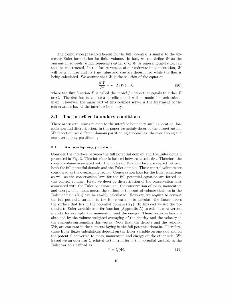
3.1.1 An overlapping partition

Consider the interface between the full potential domain and the Euler domainpresented in Fig. 3. This interface is located between tetrahedra. Therefore thecontrol volume associated with the nodes on this interface are shared betweenboth the full potential domain and the Euler domain. These control volumes areconsidered as the overlapping region. Conservation laws for the Euler equationsas well as the conservation laws for the full potential equation are forced onthis control volume. First, we describe discretization of the conservation lawsassociated with the Euler equations, i.e., the conservation of mass, momentumand energy. The fluxes across the surface of the control volume that lies in theEuler domain (ΩE) can be readily calculated. However, we require to convertthe full potential variable to the Euler variable to calculate the fluxes acrossthe surface that lies in the potential domain (ΩΦ). To this end we use the po-tential to Euler variable transfer function (Appendix A) to calculate, at vertex,k and l for example, the momentum and the energy. These vertex values areobtained by the volume weighted averaging of the density and the velocity inthe elements surrounding this vertex. Note that, the density and the velocity,∇Φ, are constant in the elements laying in the full potential domain. Therefore,these Euler fluxes calculations depend on the Euler variable on one side and onthe potential converted to mass, momentum and energy on the other side. Weintroduce an operator Q related to the transfer of the potential variable to theEuler variable defined as

U = Q(Φ). (21)

10

ΓE

ΓΦ

interface ΓI

Euler domain ΩE

full potentialdomain ΩΦ

Uo

Un

Um, Φm

ΦlΦk

Uj , Φj

Ui,Φi

Figure 3: Overlapping interface of the Euler and full potential domains.

The interface condition for the Euler solver becomes∫ΓE

F (U) · nEdS +∫

ΓΦ

F (Q(Φ)) · nΦdS = 0, (22)

where the subscript E and Φ refer to the Euler and the potential segments ofthe control volume, respectively.

Second, we present the conservation of mass for the same control volumerequired for the full potential solver. To be more precise the conservation ofmass is written as ∫

ΓE

ρV · nEdS +∫

ΓΦ

ρ∇Φ · nΦdS = 0, (23)

where ρV is the first component of the Euler flux vector. These two integralscan be discretized into sums over the edges of the control volume, such as,

∑τh

i,j

ρV · SEi,j +

∑τh

i,j

ρi,j(∇Φ)i,j · SΦi,j = 0, (24)

11

interface ΓI

full potentialdomain ΩΦ

Euler domain ΩE

Figure 4: Non–overlapping interface of the Euler and full potential domains.

where Si,j is the surface intergal of the outward normal vector along the jsurface of the control volume τc

j associated with each element τhi,j . Note that

in this approach we have over-determined the conservations laws. Indeed, thesame control volume will satisfy the conservation of mass for both the Eulerequations and for the full potential equation.

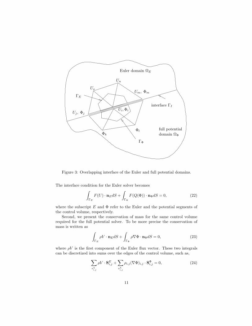
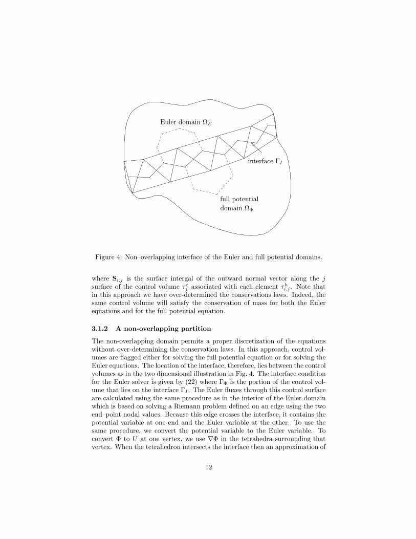
3.1.2 A non-overlapping partition

The non-overlapping domain permits a proper discretization of the equationswithout over-determining the conservation laws. In this approach, control vol-umes are flagged either for solving the full potential equation or for solving theEuler equations. The location of the interface, therefore, lies between the controlvolumes as in the two dimensional illustration in Fig. 4. The interface conditionfor the Euler solver is given by (22) where ΓΦ is the portion of the control vol-ume that lies on the interface ΓI . The Euler fluxes through this control surfaceare calculated using the same procedure as in the interior of the Euler domainwhich is based on solving a Riemann problem defined on an edge using the twoend–point nodal values. Because this edge crosses the interface, it contains thepotential variable at one end and the Euler variable at the other. To use thesame procedure, we convert the potential variable to the Euler variable. Toconvert Φ to U at one vertex, we use ∇Φ in the tetrahedra surrounding thatvertex. When the tetrahedron intersects the interface then an approximation of

12

the velocity is used instead of ∇Φ.The mass flux balance for the full potential control volume that lies on the

interface is given by (23) where ΓE is now the portion of the control volume thatlies on the interface. The term ρV is the type first term in the Euler flux vectorwhich is related to the conservation of mass. Clearly, this approach guaranteesthat the mass fluxes at the interface are conserved.

4 Computational results

4.1 Transonic flow passing a NACA0012 airfoil

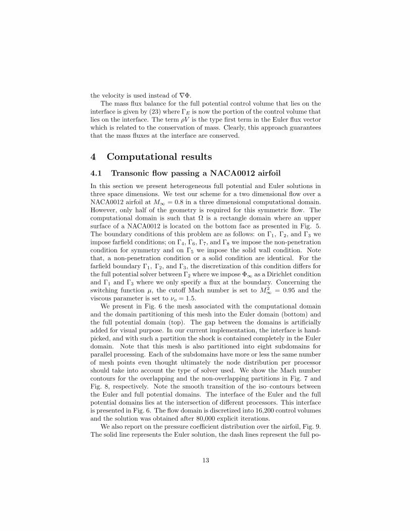
In this section we present heterogeneous full potential and Euler solutions inthree space dimensions. We test our scheme for a two dimensional flow over aNACA0012 airfoil at M∞ = 0.8 in a three dimensional computational domain.However, only half of the geometry is required for this symmetric flow. Thecomputational domain is such that Ω is a rectangle domain where an uppersurface of a NACA0012 is located on the bottom face as presented in Fig. 5.The boundary conditions of this problem are as follows: on Γ1, Γ2, and Γ3 weimpose farfield conditions; on Γ4, Γ6, Γ7, and Γ8 we impose the non-penetrationcondition for symmetry and on Γ5 we impose the solid wall condition. Notethat, a non-penetration condition or a solid condition are identical. For thefarfield boundary Γ1, Γ2, and Γ3, the discretization of this condition differs forthe full potential solver between Γ2 where we impose Φ∞ as a Dirichlet conditionand Γ1 and Γ3 where we only specify a flux at the boundary. Concerning theswitching function µ, the cutoff Mach number is set to M2

∞ = 0.95 and theviscous parameter is set to νo = 1.5.

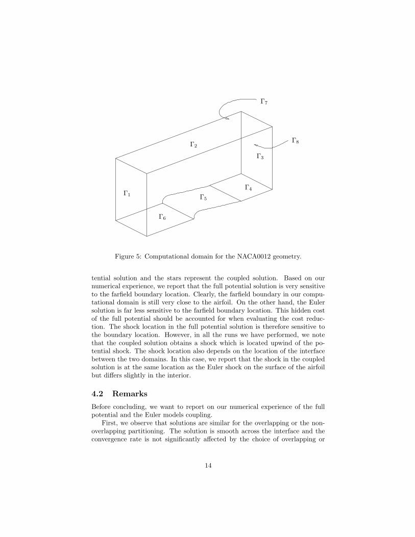
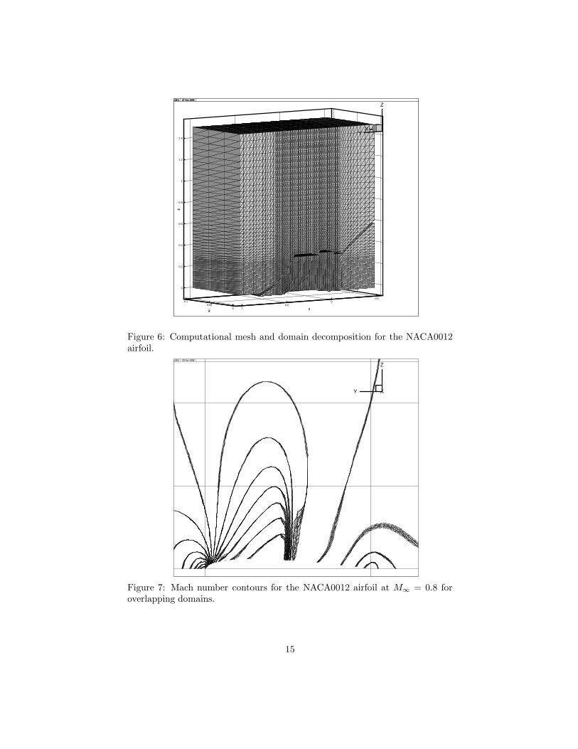
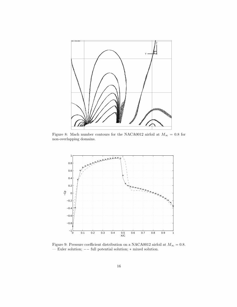
We present in Fig. 6 the mesh associated with the computational domainand the domain partitioning of this mesh into the Euler domain (bottom) andthe full potential domain (top). The gap between the domains is artificiallyadded for visual purpose. In our current implementation, the interface is hand-picked, and with such a partition the shock is contained completely in the Eulerdomain. Note that this mesh is also partitioned into eight subdomains forparallel processing. Each of the subdomains have more or less the same numberof mesh points even thought ultimately the node distribution per processorshould take into account the type of solver used. We show the Mach numbercontours for the overlapping and the non-overlapping partitions in Fig. 7 andFig. 8, respectively. Note the smooth transition of the iso–contours betweenthe Euler and full potential domains. The interface of the Euler and the fullpotential domains lies at the intersection of different processors. This interfaceis presented in Fig. 6. The flow domain is discretized into 16,200 control volumesand the solution was obtained after 80,000 explicit iterations.

We also report on the pressure coefficient distribution over the airfoil, Fig. 9.The solid line represents the Euler solution, the dash lines represent the full po-

13

Γ1

Γ2

Γ3

Γ4

Γ5

Γ6

Γ7

Γ8

Figure 5: Computational domain for the NACA0012 geometry.

tential solution and the stars represent the coupled solution. Based on ournumerical experience, we report that the full potential solution is very sensitiveto the farfield boundary location. Clearly, the farfield boundary in our compu-tational domain is still very close to the airfoil. On the other hand, the Eulersolution is far less sensitive to the farfield boundary location. This hidden costof the full potential should be accounted for when evaluating the cost reduc-tion. The shock location in the full potential solution is therefore sensitive tothe boundary location. However, in all the runs we have performed, we notethat the coupled solution obtains a shock which is located upwind of the po-tential shock. The shock location also depends on the location of the interfacebetween the two domains. In this case, we report that the shock in the coupledsolution is at the same location as the Euler shock on the surface of the airfoilbut differs slightly in the interior.

4.2 Remarks

Before concluding, we want to report on our numerical experience of the fullpotential and the Euler models coupling.

First, we observe that solutions are similar for the overlapping or the non-overlapping partitioning. The solution is smooth across the interface and theconvergence rate is not significantly affected by the choice of overlapping or

14

(3D) 27 Oct 1998

0

0.2

0.4

0.6

0.8

1

1.2

1.4

Z

00.05

0.1

X

-0.50

0.51 Y

XY

Z(3D) 27 Oct 1998

Figure 6: Computational mesh and domain decomposition for the NACA0012airfoil.

(3D) 29 Oct 1998

XY

Z(3D) 29 Oct 1998

Figure 7: Mach number contours for the NACA0012 airfoil at M∞ = 0.8 foroverlapping domains.

15

(3D) 29 Oct 1998

XY

Z(3D) 29 Oct 1998

Figure 8: Mach number contours for the NACA0012 airfoil at M∞ = 0.8 fornon-overlapping domains.

0 0.1 0.2 0.3 0.4 0.5 0.6 0.7 0.8 0.9 1−1

−0.8

−0.6

−0.4

−0.2

0

0.2

0.4

0.6

0.8

1

X/C

−Cp

Figure 9: Pressure coefficient distribution on a NACA0012 airfoil at M∞ = 0.8.— Euler solution; −− full potential solution; ∗ mixed solution.

16

non-overlapping approaches. The main difference is the added computationalcost of calculating the Euler fluxes for the overlapping control volume and thestorage associated with the existence of the overlapping control volume whichhas both the Euler variable and the potential variable. On the other hand theoverlapping partitioning is required in implicit solutions using an overlappingSchwarz algorithm.

Second, for simplicity of presentation, the discretization presented herein hasfocused on the first order scheme for the Euler equations and for the interfacediscretization. For higher order schemes, we convert from potential to the Eulervariable not only the vertex values of the control volume located on the interfacebut also the vertices of the neighbors such that the evaluation of the gradientof the solution at each vertex can be calculated. Indeed, the results presentedin Section 4 are obtained using a second order scheme. A similar approach willbe required when attempting the coupling with the Navier-Stokes equations.

Lastly, physical solutions for the full potential flow over a wing are obtainedby imposing the Kutta condition; that the flow leaves the trailing edge smoothly.For a full potential solver such a condition is enforced by adding a jump inthe potential equal to the circulation. Note that for non-lifting airfoils, as inour model problem, we do not need to enforce the Kutta condition. However,it is fortunate that the Euler solution of such flows intrinsically respects thiscondition. For future considerations such as lifting wings we will define the Eulerdomain to cover the wing and the wake region. With this partition we avoid anyspecial treatment in the full potential domain because the full potential regiondoes not cross the trailing edge vortex sheet.

5 Conclusions

In this paper we have showed the feasibility of coupling the Euler equations andthe full potential equation in the simulations of three dimensional steady com-pressible flows. An explicit formulation was presented based on a forward Eulertime integration scheme and a fully unstructured finite volume scheme for thespatial variables. Numerical results obtained on a distributed memory paral-lel computer were reported for a transonic flow passing a NACA0012 wing. Wehave also laid down the background to fully extend this formulation for multipleflow models and for different numerical approaches. We have not investigatedthe reduction in computation time because the fastest solvers are based on im-plicit approaches. The next step is to expand this formulation to the implicitapproach and address the evaluation of computation time reduction as well asother parallel implementation issues.

17

6 Acknowledgments

We thank D. Keyes and D. P. Young for many stimulating discussions.

References

[1] M. E. Berkman, L. N. Sankar, C. R. Berezin, and M. S. Torok. Navier–Stokes/full potential/free–wake method for rotor flows. J. of Aircraft,34:635–640, 1997.

[2] M. Bristeau, R. Glowinski, J. Periaux, P. Perrier, O. Pironneau, andC. Poirier. On the numerical solution of nonlinear problems in fluid dynam-ics by least squares and finite element methods (ii), application to transonicflow simulations. Comput. Methods. Appl. Mech. Engrg., 51:363–394, 1985.

[3] X.-C. Cai, C. Farhat, and M. Sarkis. A minimum overlap restricted ad-ditive Schwarz preconditioner and applications in 3D flow simulations. InC. Farhat J. Mandel and X.-C. Cai, editors, The Tenth International Con-ference on Domain Decomposition Methods for Partial Differential Equa-tions. AMS, 1998.

[4] X.-C. Cai, W. D. Gropp, D. E. Keyes, R. G. Melvin, and D. P. Young.Parallel Newton–Krylov–Schwarz algorithms for the transonic full potentialequation. SIAM J. Sci. Comput., 19:246–265, 1998.

[5] C. Coclici and W. L. Wendland. Domain decomposition methods andfarfield boundary conditions for 2D compressible viscous flows. In Proc.of ECCOMAS 98, 1998.

[6] R. Cummings, Y. Rizk, L. Schiff, and N. Chaderjian. Navier–Stokes pre-dictions for the F–18 wing and fuselage at large incidence. J. of Aircraft,29:565–574, 1992.

[7] C. Farhat and S. Lanteri. Simulation of compressible viscous flows ona variety of MPPs: Computational algorithms for unstructured dynamicmeshes and performance results. Comput. Methods Appl. Mech. Engrg,119:35–60, 1994.

[8] C. Farhat, M. Lesoinne, P. S. Chen, and S. Lanteri. Parallel heteroge-neous algorithms for the solution of the three–dimensional transient cou-pled aeroelastic problems. AIAA Paper 95-1290, 1995.

[9] W. G. Habashi and M. M. Hafez. Finite element solutions of transonic flowproblems. AIAA J., 20:1368–1375, 1982.

18

[10] M. Hafez, J. South, and E. Murman. Artificial compressibility methodfor numerical solution of the transonic full potential equation. AIAA J.,17:838–844, 1979.

[11] C. Hirsch. Numerical Computation of Internal and External Flows. JohnWiley and Sons, New York, 1990.

[12] T. L. Holst and W. F. Ballhaus. Fast, conservative schemes for the fullpotential equation applied to transonic flows. AIAA J., 17:145–152, 1979.

[13] T. L. Holst, J. W. Slooff, H. Yoshihara, and W. F. Ballhaus. Applied com-putational transonic aerodynamics. Technical Report AG-266, AGARD,1982.

[14] A. Jameson. Essential elements of computational algorithms for aerody-namics. Technical Report 97-68, ICASE, 1997.

[15] A. Jameson, T. Baker, and N. Weatherill. Calculation of inviscid transonicflow over a complete aircraft. AIAA Paper 86-0103, 1986.

[16] B. Van Leer. Towards the ultimate conservative difference scheme. V. Asecond order sequel to Godunov’s method. J. Comput. Phys., 32:361–370,1979.

[17] M. Paraschivoiu, X.-C. Cai, M. Sarkis, D. P. Young, and D. Keyes. Animplicit multi–model compressible flow formulation based on the full po-tential equation and the Euler equations. AIAA Paper 99-0784, 1999. Toappear.

[18] R. B. Pelz and A. Jameson. Transonic flow calculations using triangularfinite elements. AIAA Paper 83–1922, 1983.

[19] A. Quarteroni and A. Valli. Domain Decomposition Methods for PartialDifferential Equations. Oxford University Press, Oxford, 1999.

[20] L. N. Sankar, B. K. Bharadvaj, and F. Tsung. Three-dimensional Navier–Stokes/full potential coupled analysis for transonic viscous flow. AIAA J.,31:1857–1862, 1993.

[21] V. Shankar, H. Ide, J. Gorski, and S. Osher. A fast, time–accurate, un-steady full potential scheme. AIAA J., 25:230–238, 1987.

[22] D. P. Young, R. G. Melvin, M. B. Bieterman, F. T. Johnson, and S. S.Samant. Global convergence of inexact Newton methods for transonic flow.Int. J. Numer. Methods. Fluids, 11:1075–1095, 1990.

[23] D. P. Young, R. G. Mervin, M. B. Bieterman, F. T. Johnson, S. S. Samant,and J. E. Bussoletti. A locally refined rectangular grid finite elementmethods: Application to computational fluid dynamics and computationalphysics. J. Comput. Phys., 92:1–66, 1991.

19

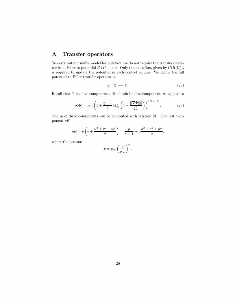
A Transfer operators

To carry out our multi–model formulation, we do not require the transfer opera-tor from Euler to potential R : U −→ Φ. Only the mass flux, given by G(R(U)),is required to update the potential in each control volume. We define the fullpotential to Euler transfer operator as

Q : Φ −→ U. (25)

Recall that U has five components. To obtain its first component, we appeal to

ρ(Φ) = ρ∞

(1 +

γ − 12

M2∞

(1 − ||∇Φ||22

q2∞

))1/(γ−1)

. (26)

The next three components can be computed with relation (3). The last com-ponent ρE

ρE = ρ

(e +

u2 + v2 + w2

2

)=

p

γ − 1+ ρ

u2 + v2 + w2

2,

where the pressure

p = p∞

(ρ

ρ∞

)γ

.

20