Submitted 18 December 2014Accepted 13 August 2015Published 3 September 2015

Corresponding authorCharles C. Frasier,frasierf@ix.netcom.com

Academic editorJohn Hutchinson

Additional Information andDeclarations can be found onpage 35

DOI 10.7717/peerj.1228

Copyright2015 Frasier

Distributed underCreative Commons CC-BY 4.0

OPEN ACCESS

An explanation of the relationshipbetween mass, metabolic rate andcharacteristic length for placentalmammalsCharles C. Frasier

San Diego, California, USA

ABSTRACTThe Mass, Metabolism and Length Explanation (MMLE) was advanced in 1984 toexplain the relationship between metabolic rate and body mass for birds andmammals. This paper reports on a modernized version of MMLE. MMLEdeterministically computes the absolute value of Basal Metabolic Rate (BMR) andbody mass for individual animals. MMLE is thus distinct from other examina-tions of these topics that use species-averaged data to estimate the parameters in astatistically best fit power law relationship such as BMR = a(bodymass)b. Beginningwith the proposition that BMR is proportional to the number of mitochondria inan animal, two primary equations are derived that compute BMR and body massas functions of an individual animal’s characteristic length and sturdiness factor.The characteristic length is a measureable skeletal length associated with an animal’smeans of propulsion. The sturdiness factor expresses how sturdy or gracile an animalis. Eight other parameters occur in the equations that vary little among animals inthe same phylogenetic group. The present paper modernizes MMLE by explicitlytreating Froude and Strouhal dynamic similarity of mammals’ skeletal musculature,revising the treatment of BMR and using new data to estimate numerical values forthe parameters that occur in the equations. A mass and length data set with 575entries from the orders Rodentia, Chiroptera, Artiodactyla, Carnivora, Perissodactylaand Proboscidea is used. A BMR and mass data set with 436 entries from the ordersRodentia, Chiroptera, Artiodactyla and Carnivora is also used. With the estimatedparameter values MMLE can calculate characteristic length and sturdiness factorvalues so that every BMR and mass datum from the BMR and mass data set canbe computed exactly. Furthermore MMLE can calculate characteristic length andsturdiness factor values so that every body mass and length datum from the massand length data set can be computed exactly. Whether or not MMLE can calculatea sturdiness factor value so that an individual animal’s BMR and body mass can besimultaneously computed given its characteristic length awaits analysis of a data setthat simultaneously reports all three of these items for individual animals. Howeverfor many of the addressed MMLE homogeneous groups, MMLE can predict theexponent obtained by regression analysis of the BMR and mass data using theexponent obtained by regression analysis of the mass and length data. This arguesthat MMLE may be able to accurately simultaneously compute BMR and mass for anindividual animal.

How to cite this article Frasier (2015), An explanation of the relationship between mass, metabolic rate and characteristic length forplacental mammals. PeerJ 3:e1228; DOI 10.7717/peerj.1228

Subjects Biophysics, Mathematical Biology, ZoologyKeywords Morphology, Basal metabolic rate (BMR), Placental mammals, Mitochondria,Froude dynamic similarity, Strouhal dynamic similarity, Body mass, Characteristic length,Sturdiness factor, Phylogenetic groups

INTRODUCTIONMost theoretical treatments of Basal Metabolic Rate (BMR) have focused on the exponent

in a relationship of the form BMR = aWb where W is body mass. Two concepts have

dominated. One concept is geometric similarity in which the value of the exponent

b = 2/3. The theoretical explanations for this value of the exponent generally involve a

balance between heat production and its loss through the body surface (Sarrus & Rameaux

in the 1830s as cited by White & Kearney, 2014; Hulbert & Else, 2004; Clarke, Rothery &

Isaac, 2010; Roberts, Lightfoot & Porter, 2010; White, 2010; Roberts, Lightfoot & Porter, 2011;

Seymour & White, 2011). In the other concept b = 3/4 (Kleiber, 1932; Kleiber, 1961). This

has been known as “Kleiber’s Law”. A theoretical explanation for b = 3/4 was proposed

based on a fractal network for a body’s resource supply system (West, Brown & Enquist,

1997; West, Brown & Enquist, 1999). More recently theoretical explanations involving

resource distribution networks for which the value of the exponent b can be as small

as 2/3 or as large as 3/4 have been proposed (Banavar et al., 2010). The metabolic-level

boundaries hypothesis proposes that the exponent b is proportional to the proportions of

influence of volume and surface area boundary constraints and thus has a value between

2/3 and 1.0 (Glazier, 2010).

More microscopically, it has been proposed that an animal’s BMR is proportional to the

total number of mitochondria in its tissues (Smith, 1956) or to the sum of the metabolic

rates of its constituent cells (Kozlowski, Konarzewski & Gawelczyk, 2003). At an even smaller

scale it has been proposed in membrane pacemaker theory (Hulbert & Else, 1999) that

BMR is governed by the degree of polyunsaturation of membrane phospholipids or, in the

Quantum Metabolism theory (Agutter & Tuszynski, 2011), by molecular-cellular processes.

Recent analyses of BMR, body mass data have argued that there is no single exponent b

that applies to a phylogenetic class such as mammals. The relationship is more complicated

than BMR = aWb (Kolokotrones et al., 2010). It has also been argued that there are different

exponents for different phylogenetic groups such as mammal orders (White, Blackburn &

Seymour, 2009; Capellini, Venditti & Barton, 2010) or different orders among insects, fish,

reptiles and birds as well as mammals (Isaac & Carbone, 2010).

The dynamic energy budget (DEB) hypothesis (Sousa et al., 2010; White et al., 2011;

Maino et al., 2014) can predict the absolute value of BMR rather than the exponent b in the

relationship aWb.

In 1984 the author of the current paper proposed the Mass, Metabolism and Length

Explanation (MMLE) theory that also predicts the absolute value of BMR rather than just

the exponent b in the relationship BMR = aWb (Frasier, 1984). A purpose of developing

MMLE theory was to relate BMR to measurable skeletal dimensions with the hope of

estimating the BMR of extinct animals. Starting with the Smith (1956) proposal that

Frasier (2015), PeerJ, DOI 10.7717/peerj.1228 2/40

an animal’s BMR is proportional to the total number of mitochondria in its tissues the

theoretical derivation took a course that resulted in equations for predicting the absolute

value of body mass as a function of a skeletal length dimension as well as predicting the

absolute value of BMR as a function of that skeletal dimension. Used together these

equations can predict the absolute value of BMR as a function of body mass. This paper

will frequently be referred to as the ‘original paper’ in the present paper.

McNab (1988) questioned what should be the best measure of body size against which

to scale various functions such as BMR. He presented good reasons why body mass is more

variable than linear dimensions in adult mammals. Nevertheless McNab concluded that he

would use body mass for want of a better measure of body size. Mass may be an even less

reliable measure of body size among bats in which it may vary by as much as 15% to 50%

daily (Iriarte-Diaz et al., 2012).

The simplest relationship between body mass and a skeletal length dimension would be

geometric similarity in which body mass would be proportional to the cube of the length

or, equivalently, the length would be proportional to the cube root of the mass. However

Galileo, as cited in Christiansen (1999) and Biewener (2005), recognized in 1638 that

geometric similarity implied that small animals would have to be mechanically overbuilt or

large animals would have to operate near the limit of mechanical failure. Elastic similarity

was proposed as a theoretical solution to this problem (McMahon, 1973; McMahon, 1975)

but its predictions did not agree with data (Alexander et al., 1979; Christiansen, 1999). More

recently an explanation based on the need of long bones to resist bending and compressive

stress has been proposed (Garcia & da Silva, 2004).

It has been recognized that in a relationship relating a skeletal length, l, to body mass

raised to an exponent, Wx, the exponent may be different for large terrestrial mammals

compared to small terrestrial mammals (Christiansen, 1999; Biewener, 2005). Campione

& Evans (2012) found that the regression between the total circumference of the humerus

and femur to body mass exhibits the strongest relationship in that the relationship has the

highest coefficient of determination values; and the lowest mean percent prediction error,

standard error of the estimate and Akaike Information Criterion values of all bivariate

regression models for extant mammals and reptiles.

These theoretical explanations for the relationship between skeletal length dimensions

and body mass are based on the stresses the bones and their supporting tissues must

accommodate. MMLE theory went in a different direction by examining the rate of energy

use in skeletal muscle tissues during activity and the relationship between muscle energy

use and energy use by a body’s other tissues in the basal metabolic rate state.

Since the original publication of MMLE the amount of BMR, body mass data has vastly

expanded as have the resources with which to analyze it. So the purpose of this paper is to

use these resources to revisit MMLE theory and test its ability to predict the absolute values

of BMR and body mass for individual animals with the new data. MMLE theory will also be

modified as necessary.

The running/walking members of the orders Artiodactyla, Carnivora, Perissodactyla

and Proboscidea were addressed in the original paper. The present analysis will add

Frasier (2015), PeerJ, DOI 10.7717/peerj.1228 3/40

Rodentia and Chiroptera (bats) as well as redo the runners/walkers analysis with new

data. Rodentia are a small animal counterbalance to the large runners/walkers and they

comprise over 40% of placental mammal species. A comprehensive theory should be able

to address flying animals as well as terrestrials and bats comprise another 20% of placental

mammal species. Swimming animals should also be addressed but there is too little BMR

and body mass data to generate reliable results for the orders Pinnipedia, Cetacea and

Sirenia. While not addressing the entirety of the placental mammals, the orders that are

addressed do represent over two-thirds of the species.

SUMMARY OF MMLE THEORYArticle S2 presents an abbreviated version of MMLE theory as originally formulated

(Frasier, 1984) together with some necessary modifications. This section is a summary

of Article S2.

Nearly all of the energy flux that is measured as basal metabolic rate (BMR) is generated

by mitochondria. Although there are other ways to measure it, BMR is most commonly

measured by oxygen consumption (Hulbert & Else, 2004). The oxygen is consumed

by processes that pump protons across the mitochondrion inner membrane. Heat is

produced when some of the protons leak back across the membrane in a controlled

fashion as in brown fat or as an uncontrolled basal leak. Otherwise the protons cause

the phosphorylation of adenosine diphosphate (ADP) to adenosine triphosphate (ATP) as

they return across the inner membrane (Jastroch et al., 2010). ATP is the fuel that powers

animal tissues.

MMLE strives to predict the absolute value of the BMR of an animal rather than the

exponent b or the constant a in the relationship aWb. It calculates BMR by summing

the energy allocation to an animal’s tissues. The energy allocated to a tissue type is

proportional to the number of mitochondria in the tissue. Thus MMLE tries to count the

mitochondria in the tissues that compose an animal and then sum these counts for the en-

tire animal. This approach to calculating an animal’s BMR was proposed by (Smith, 1956).

It is a signature feature of MMLE theory that the vertebrate body is represented

as a combination of masses instead of a single mass. There are at least two masses:

(1) the skeletal musculature which is governed by dynamic similarity and in which

the mitochondria are approximately uniformly distributed; and (2) the non-skeletal

musculature in which the mitochondria are concentrated in surfaces that surround

material with few mitochondria. The heart, kidneys, liver and brain are the principal

non-skeletal muscle tissues.

Being a surface, the non-skeletal muscle surface can be mathematically described as

the square of a length multiplied by an appropriate constant. Any length could be used

as long as the constant is adjusted to make the relationship exact. For MMLE theory the

selected length is one that is related to propulsion dynamics. This selected length is called

the ‘characteristic length’, l. The proportionality constant includes the ‘sturdiness factor’, s. s

is non-dimensional.

Frasier (2015), PeerJ, DOI 10.7717/peerj.1228 4/40

In Article S1 an equation is derived for an animal’s body mass, W , in terms of l and s:

W = (sl)2Gm/kfe + ((sl)2mGo/e)1/y. (1)

Also an equation is derived for an animal’s BMR in terms of l and s:

BMR = Gr(sl)2 (2)

Gm/k is the skeletal muscle mass constant. Go is the non-skeletal muscle constant. Gr is the

resting metabolic rate constant. Gm, Go and Gr are universal constants that should apply to

all vertebrates. y is the non-skeletal muscle mass exponent. m is a dimensionality factor that

adjusts the physical dimensions of this expression to mass. m is determined by y. y and m

should have the same value for all animals in a phylogenetic group. k is the locomotion

constant. k is a function of the type of dynamic similarity that applies to the type of

propulsion used by an animal. k should be similar for all vertebrates that are dynamically

similar. The fundamental propulsion frequency, f , should be the same function of the

characteristic length, l, for all vertebrates that are dynamically similar. The mitochondrion

capability coefficient, e, is a constant whose value should be approximately identical for all

vertebrates in the same phylogenetic group with the same body temperature. The charac-

teristic length, l, and the sturdiness factor, s, have unique values for each individual animal.

Go is defined so that m is dimensionless with a value of 1.0 for geometrically similar

non-skeletal musculature for which y = 2/3. Gm and k were defined so that k is

non-dimensional with a value of 1.0 for running/walking placental mammals.

After analyzing data for running/walking mammals, rodents and bats a general

formulation for the fundamental propulsion frequency appears to be f = c/lr where c is the

propulsion frequency proportionality constant and r is the propulsion frequency exponent

with a value between 0.5 and 1.0 for species in these mammal orders. Substituting this

expression for f in Eq. (1) yields:

W = s2l(2+r)Gm/kce + ((sl)2mGo/e)1/y (3)

Animals that are dynamically similar have similar values for the exponent, r.

When the gravitational force dominates the dynamics of animals’ movement, two

animals are dynamically similar when the ratio of gravitational force to inertial force is

the same at corresponding stages of their motions. The animals are Froude similar and

they have equal Froude numbers, F, where F = u2/gl and u is speed, l is the characteristic

length and g is the acceleration of gravity (Alexander & Jayes, 1983; Alexander, 2005).

Running/walking mammals are Froude similar (Alexander et al., 1979; Alexander, 2005;

Raichlen, Pontzer & Shapiro, 2013).

Strouhal similarity obtains when inertial forces are proportional to oscillatory forces.

Similarity implies equal Strouhal numbers, St, where St = fl/u and f is the frequency, l is

the characteristic length and u is speed. The Strouhal number governs a series of vortex

growth and shedding regimes for foils undergoing pitching and heaving motions thereby

describing the tail or wing kinematics of swimming or flying animals (Taylor, Nudds &

Thomas, 2003).

Frasier (2015), PeerJ, DOI 10.7717/peerj.1228 5/40

Reynolds similarity obtains when inertial forces are proportional to viscous forces.

Similarity implies equal Reynolds numbers, R, where R = ulρ/ν and u is speed, l is

characteristic length, ρ is fluid density and ν is fluid viscosity (Alexander, 2005). Bats

are the only animals examined in the present paper for which viscous drag, and hence

Reynolds similarity, might be important. Strouhal similarity does apply to bats. If both

Reynolds and Strouhal similarity simultaneously apply, then by solving for speed, u, in the

definitions of Reynolds and Strouhal numbers, the frequency, f , is seen to be proportional

to the inverse of the characteristic length squared, or f = Rν/Stρl2. This sort of dependence

of the frequency on the characteristic length was not observed. It should be noted, however,

that the characteristic length for viscous drag and that for vortex growth and shedding

could be different body dimensions.

Two animals are geometrically similar if one can be made identical to the other by

multiplying all its linear dimensions by the same factor (Alexander, 2005). Properties

of geometric similarity include surface area, S, being proportional to the square of the

characteristic length, l2, and simultaneously volume, V , being proportional to the cube

of the characteristic length, l3. Since mass, W , is proportional to volume, mass is also

proportional to l3. From Eq. (3) geometric similarity of the skeletal musculature means

that the fundamental propulsion frequency exponent r = 1.0. The fundamental frequency

constant, c, in Eq. (3) has the dimension of speed. If the non-skeletal musculature is also

geometrically similar with y = 2/3, then the entire animal will be geometrically similar.

Froude and Strouhal dynamic similarity are separately compatible with geometric

similarity.

If both Froude and Strouhal similarity simultaneously apply then equating speed in

the definitions of the Froude and Strouhal numbers results with the frequency, f , being

proportional to the pendulum frequency, (g/l)0.5. Substituting this expression for f in

Eq. (1) shows that mass, W , is not proportional to l3 and thus geometric similarity does not

apply. From Eqs. (2) and (3) geometric similarity means that BMR is proportional to body

mass raised to the 2/3 power, W2/3. Simultaneous Froude and Strouhal similarity implies

that BMR is proportional to body mass raised to a power greater than 2/3.

Hereafter, when it is stated that geometric similarity applies it also means that either

Froude or Strouhal dynamic similarity also applies.

The sturdiness factor is best understood by looking at Fig. 1. Figure 1 plots 314 samples

of log body mass versus log shoulder height for running/walking mammals from the

orders Artiocactyla and Carnivora obtained from (Nowak, 1999). Shoulder height is a

good surrogate for characteristic length for running/walking mammals. The data in Fig. 1

spread over an area in the two dimensional log shoulder height, log body mass space. It

was found in the original paper that most of the area over which the data spreads would

be bounded by an upper line computed using Eq. (3) with the sturdiness factor set to the

square root of 3, (3)0.5, and a lower line computed with the sturdiness factor set to (3)−0.5.

These boundaries are plotted as the upper and lower slanting lines in Fig. 1. Excluding

Hippopotamus amphibius and domestic cattle, over 97% of the data plotted in Fig. 1 are

contained between these boundary lines.

Frasier (2015), PeerJ, DOI 10.7717/peerj.1228 6/40

Figure 1 Log body mass as a function of log shoulder height for running/walking Artiodactyla andCarnivora. Data are from Nowak (1999). The upper and lower slanted solid lines are MMLE sturdinessfactor boundaries for y = 2/3. The upper boundary was generated with a sturdiness factor, s, of thesquare root of 3, (3)0.5. The lower boundary was generated with s = (3)−0.5. The middle slanted line wasgenerated with s = 1.0. The slanted lines are for Froude–Strouhal dynamic similarity. The Artiodactylamass and shoulder height data are marked by open squares. The Carnivora mass and shoulder height dataare marked by open triangles. Excluding Hippopatamus amphibus marked by crossed Xes and domesticcattle marked by Xes, R2

M = 0.9997. The solid vertical lines demark the AVG method first set of cohorts.The dashed vertical lines demark the second set of cohorts.

The data bordering the upper line are for sturdy animals such as a large American

black bear (Ursus americanus) with W = 270 kg, l = 0.91 m and s = 1.63 or a large

water chevrotain (Hyemoschus aquaticus) with W = 15 kg, l = 0.355 m and s = 1.35.

The data bordering the lower are for gracile animals such as a small bob cat (Felis rufus)

with W = 4.1 kg, l = 0.45 m and s = 0.556 or a large roe deer (Capreolus pygargus) with

W = 50 kg, l = 1.0 m and s = 0.687. (Note that posture and limb design do not necessarily

reflect the concept of ‘gracile’ as used herein.) At the same characteristic length an animal

with a greater sturdiness factor is more massive than an animal with a lesser sturdiness

factor—hence the nomenclature ‘sturdiness’ factor.

Frasier (2015), PeerJ, DOI 10.7717/peerj.1228 7/40

MATERIALS AND METHODSSurrogate characteristic length and body mass data are available in Nowak (1999). It has

been entered into Microsoft Excel spreadsheets that are available as Data S1, Data S2

and Data S3. The author of the present paper is unaware of any substantial collection

of BMR and characteristic length data. There is substantial BMR and body mass data in

McNab (2008). These data are also available with additional data as a Microsoft Excel

spreadsheet in the Supplementary Information for Kolokotrones et al. (2010) at www.

nature.com/nature/journal/v464/n7289/suppinfo/nature08920.html which was the source

that was used for the present paper. To use this data, Eqs. (1) and (2) can be used together

to numerically express BMR as a function of body mass.

For running/walking placental mammals 226 individual mass and shoulder height

samples were obtained for Artiodactyla (Data S1). Hippopotamus amphibius and Bos

Taurus (aurochs and domestic cattle) were excluded from the analysis. Aurochs are extinct

and domestic cattle have been bred for human purposes rather than survival in the wild.

H. amphibius is an amphibious animal well suited to a semi aquatic existence. It is a poor

swimmer. It uses a means of locomotion in water that is quite different from that used by

other amphibious mammals. Submerged, it runs/walks on the bottom of the body of water

through which it is traveling (Nowak, 1999). Buoyancy alters the ratio of gravitational force

to inertial force making similarity of H. amphibius with more terrestrial runners/walkers

suspect.

84 individual mass and shoulder height samples were obtained for Carnivora (Data S1).

The Mustelidae were mostly excluded because shoulder height was not given except for

wolverines (Gulo gulo) and honey badgers (Mellivora capensis). Shoulder height was not

given for most of the smaller Carnivora so that the smallest sample was a raccoon (Procyon)

with a mass of 2,000 g and a shoulder height of 0.228m.

26 individual mass and shoulder height samples were obtained for Perissodactyla. Eight

individual samples were obtained for Proboscidea (Data S1).

To do Phylogenetically Informed (PI) regression analyses, the individual samples were

species-averaged resulting in 129 artiodactyl, 43 carnivoran, 14 perissodactyl and three

proboscid species-averaged samples. The BMR and body mass species-averaged data set

contained 20 samples for Artiodactyla and 58 samples for Carnivora.

For Rodentia (Nowak, 1999) provides individual data on approximate minimum and

maximum masses in grams (g) and head and body lengths in millimeters (mm). The length

data are mostly for genera with very little data for species. There is also very little data

on shoulder height. 203 individual and 105 taxon-averaged mass, head and body length

samples were obtained (Data S2). Kolokotrones et al. (2010) provides 267 species-averaged

BMR in watts (W) and mass in grams (g) samples.

For Chiroptera (bats) (Nowak, 1999) provides data in grams for approximate minimum

and maximum body masses. It also provides in millimeters approximate head and body

lengths, forearm lengths and tail lengths when a tail is present. The data are mostly for

genera with very little data for species. There is little data on wing span. 350 individual and

176 taxon-averaged body mass, head and body length and forearm length samples were

Frasier (2015), PeerJ, DOI 10.7717/peerj.1228 8/40

obtained (Data S3). 85 species-averaged BMR and body mass samples were obtained. BMR

is given in watts and mass is given in grams.

Determining numerical values for the universal constants Gm, Go and Gr requires three

equations. Since Eq. (3) is just a version of Eq. (1) another equation is required. Numerical

values for the constants Gm and Go could be obtained by solving Eq. (3) for two different

samples of body mass and characteristic length, l. MMLE uses a more general approach.

An approximation to Eqs. (1) and (3) is:

W = dlx (4)

x is the approximate mass exponent and d is the approximate mass multiplicative constant.

This expression is useful for establishing the approximate relationship between body mass,

W , and characteristic length, l, by regression analysis of W,l data for a group of animals.

For least squares regression a figure of merit for how well the expression represents the

data is the coefficient of determination, R2. The coefficient of determination measures the

fraction of the dependent variable’s variance that is explained by the expression.

Least squares regression is performed on the logarithmic version of Eq. (4), log(W) =

log(d) + xlog(l), to obtain best estimate values for log(d) and x.

Another useful expression is obtained by equating the derivatives with respect to log(l)

of the logarithms of Eqs. (3) and (4) to obtain, for s = 1.0 and geometrically similar

non-skeletal musculature where y = 2/3, an equation for the exponent x in Eq. (4):

x = 2.0 + r + (1 − r)(Go/e)3/2/(l(r−1)Gm/kec + (Go/e)3/2) (5)

Eq. (5) is the third equation needed to establish numerical values for the universal

constants Gm, Go and Gr.

The usual way to get the best estimate value for the parameter x in equations like

Eq. (4) has been by regression analysis of the logarithmic version of the equation. The

analyses have used species-averages in which a datum is the average value for a collection

of individuals from a single species. In ordinary least squares (OLS) and reduced major

axis (RMA) regression analyses it has been assumed that the species-averaged data are

statistically independent. Phylogenetically informed (PI) analyses assume that the data are

not independent but covary with the degree of phylogenetic relatedness between species.

These regression methods are reviewed in detail by (White & Kearney, 2014).

By Eqs. (2) and (3) MMLE deterministically computes the absolute value of BMR

and body mass for individual samples rather than a statistical best fit average value for a

collection of individuals from a single species. MMLE is thus compatible with data sets

that contain individual animal data. It is also compatible with species-averaged data sets

by considering each species-averaged datum to correspond with at least one individual

member of the species.

If a group of animals have nearly identical values for all the parameters occurring in

Eqs. (2) and (3) except for characteristic length, l, and sturdiness factor, s, then BMR and

body mass can be regressed on characteristic length with sturdiness factor boundaries

Frasier (2015), PeerJ, DOI 10.7717/peerj.1228 9/40

as illustrated in Fig. 1. As long as the only parameters in Eq. (2) and (3) that distinguish

one individual animal from another are characteristic length and sturdiness factor the

individuals included in the analysis may be from different species, genera, families, and

even orders. Such a group of animals is called a MMLE homogeneous group herein.

The AVG regression method exploits this feature of MMLE to use individual animal data

such as the unmodified data from Nowak (1999). The AVG regression method is unique to

MMLE. A detailed explanation of the method is given in Article S1.

The appendix to the original paper shows that the OLS regression relationship between

body mass and characteristic length is given by the equivalent of Eq. (3) evaluated with a

sturdiness factor value of s = 1.0 for a MMLE homogeneous group. The s = 1.0 regression

relationship is plotted by the middle slanting line in Fig. 1. For any particular characteristic

length, the mean of the logs of all body masses with that characteristic length that are

uniformly distributed between the upper and lower sturdiness factor boundaries is the

log of the body mass computed by Eq. (3) evaluated with a sturdiness factor of s = 1.0.

Using the AVG regression method, MMLE takes advantage of this property to get linear

regression relationships between log body mass regressed on log characteristic length with

coefficients of determination, R2, that are very nearly 1.0.

The next section describes using the AVG regression method on characteristic length,

body mass data for running/walking placental mammals in the orders Artiodactyla and

Carnivora from Nowak (1999) to estimate numerical values for the parameter x in Eqs. (4)

and (5) and then the parameters Gm/k and Go in Eqs. (1) and (3). The numerical values for

Gm/k and Go apply to all placental mammals.

BMR and characteristic length data to estimate a numerical value for the parameter Gr

in Eq. (2) was unavailable. Species-averaged BMR and body mass data was available from

Kolokotrones et al. (2010).

By Eqs. (2) and (4),

BMR = Gr(W/d)2/x. (6)

Since d and x are estimated by regression analysis this expression is reliable only if the

coefficient of determination, R2, is nearly unity for the analysis that estimated d and x. In

the next section it is shown that R2= 0.9932 for the AVG regression analysis that estimated

d and x for running/walking placental mammals in the orders Artiodactyla and Carnivora.

Although there are complications that will be discussed in the next section a reasonable

estimate for the numerical value of Gr is obtained.

To solve for a numerical value of Gr an allometric expression of the form BMR = aWb is

obtained by regression analysis. If Eq. (6) is reliable then b = 2/x and a = Gr/d2/x.

Phylogenetically Informed (PI) Generalized Least Squares regression was used to obtain

the needed BMR = aWb expression. The PI Generalized Least Squares regression analyses

were conducted using the BayesTraits computer program (Pagel, Meade & Barker, 2004). PI

methods are used to control for an assumed lack of statistical independence among species

(Freckleton, Harvey & Pagel, 2002; White & Kearney, 2014).

Frasier (2015), PeerJ, DOI 10.7717/peerj.1228 10/40

The Microsoft Windows version of BayesTraits together with the companion programs

BayesTrees and BayesTreesConverter available at www.evolution.rdg.ac.uk were used. For

Rodentia and bats the all mammals phylogenetic tree that is available as supplemental

information from the online version of Fritz, Bininda-Emonds & Purvis (2009) at http:

//onlinelibrary.wiley.com/doi/10.111/j.1461-0248.2009.01307.x.suppinfo was used. For

running/walking mammals the updated tree for Carnivora that is available from the online

version of Nyakatura & Bininda-Emonds (2013) at www.ncbi.nlm.nih.gov/pmc/articles/

PMC3307490/ was grafted onto the all mammals tree. The analyses were performed with

the continuous regression model and maximum likelihood analysis type. The inputs were

set to estimate the parameter lambda (see Article S1).

Lambda is found by maximum likelihood. It usually varies between 0.0 and 1.0

indicating increasing phenotypic similarity with increasing phylogenetic relatedness.

It is a multiplier of the off-diagonal elements of the Generalized Least Squares

variance–covariance matrix. Lambda = 0.0 indicates evolution of traits that is independent

of phylogeny, while lambda = 1.0 indicates that traits are evolving according to Brownian

motion. Intermediate values indicate that traits have evolved according to a process

in which the effect of phylogeny is weaker than in the Brownian model (Pagel, 1999;

Freckleton, Harvey & Pagel, 2002; Pagel, Meade & Barker, 2004; Capellini, Venditti & Barton,

2010). BayesTraits results generated with lambda = 0.0 are the same as those obtained with

Ordinary Least Squares (OLS) linear regression. Results generated with lambda = 1.0 are

the same as those generated by phylogenetically independent contrasts (Capellini, Venditti

& Barton, 2010). Occasionally lambda was estimated to be greater than 1.0. This can be

interpreted as traits that are more similar than what is predicted by Brownian motion

(Freckleton, Harvey & Pagel, 2002).

Since BayesTraits estimates maximum likelihood for a hypothesis (such as the applicable

value of lambda), the log likelihood ratio for two hypotheses can be computed. By

convention a value of 4.0 or greater for the ratio is taken as evidence that one of the

hypotheses explains the data significantly better than the other (Pagel, 1999).

PI regression analyses were performed for both BMR regressed on body mass and

body mass regressed on characteristic length. The species-averaged BMR, body mass

data from Kolokotrones et al. (2010) was inputted directly to BayesTraits. The body mass,

characteristic length data from Nowak (1999) are mostly maximum and minimum

measurements of individuals from the same species or genera in which a datum is the

measurements for the largest or smallest individual measured in the taxon. Body mass,

characteristic length data were taxon-averaged before being inputted to BayesTraits.

Together with the dynamic similarity implied by the mode of locomotion for a group of

animals, PI regression relationships are helpful for partitioning populations into MMLE

homogeneous groups to which the AVG regression technique can be applied as when a

geometrically similar partition can be identified by a log(mass) regressed on log(length)

slope of 3.0 or a log(BMR) regressed on log(mass) slope of 2/3. Since the only parameters

in Eq. (3) that differ between individual members of a MMLE homogeneous group are the

Frasier (2015), PeerJ, DOI 10.7717/peerj.1228 11/40

characteristic length, l, and the sturdiness factor, s, further consideration of the relatedness

of members should not be necessary to use Eq. (3).

Regression analysis measures the error for a datum as the distance between the datum

and a line established by the regression analysis. The line minimizes the sum of the squares

of the errors.

In MMLE theory the OLS regression line can be replaced by a ‘band’. The band is

the area enclosed by the sturdiness factor boundaries. Recognizing this fact, R2 can be

replaced by a MMLE version that is denoted “R2M”. R2

M is computed in the same ways as

R2 except that the ‘error’ for a datum that falls between the sturdiness factor boundaries

is zero and the ‘error’ for a datum that falls outside the sturdiness factor boundaries is the

distance between the datum and the nearest sturdiness factor boundary. R2M is interpreted

as a measure of how well data clusters within the area bounded by the sturdiness factor

boundaries. R2M is useful for estimating values for the parameters that appear in Eq. (3)

when they may differ from the values established for running/walking placental mammals.

Excluding Hippopotamus amphibius and domestic cattle, R2M = 0.9997 for the data in

Fig. 1. R2M is very nearly unity because the data considered in the present paper mostly lie

between the sturdiness factor boundaries or very near to a boundary. Coverage, R, which is

the fraction of the data that lies between the boundaries, is another figure of merit that is

usually smaller than R2M · R = 0.9774 for the data in Fig. 1.

By examining individual animal metabolic rates and masses, Hudson, Isaac & Reuman

(2013) recently reported substantial metabolic rate heterogeneity at the species level

and commented that this is a fact that cannot be revealed by species-averaged data

sets. It was further commented that individual data might be more important than

species-averaged data in determining the outcome of ecological interactions and hence

selection. Heterogeneity is predicted by Eqs. (2) and (3) due to variation of characteristic

length and sturdiness factor among the individuals composing a species. The AVG

regression method is compatible with species level heterogeneity.

Sturdiness factor boundaries and R2M can also apply to the BMR, body mass data

from Kolokotrones et al. (2010). The boundaries are calculated by using Eq. (3) with

the bounding sturdiness factors to calculate the body mass and using Eq. (2) with the

bounding sturdiness factors to calculate the BMR for characteristic lengths that span the

range of interest. The associated value of R2M can then computed using the BMR as a

function of body mass boundaries.

The calculated numerical values reported in the present paper are given with four

significant digits to the right of the decimal point. It is suspected that the data used is not

accurate enough to support this precision.

RUNNING/WALKING PLACENTAL MAMMALS RESULTSThis is an abbreviated version of the analysis of running/walking placental mammals. The

detailed analysis is available in Article S1.

The original paper established the numerical values for the constants in the MMLE

equations by AVG analysis of 163 samples of the running/walking members of the

Frasier (2015), PeerJ, DOI 10.7717/peerj.1228 12/40

orders Artiodactyla, Carnivora, Perrisodactyla and Proboscidea from Walker (1968).

The four orders were analyzed together as a MMLE homogeneous group because their

mode of locomotion was similar and it was expected that they would be dynamically

similar so that the fundamental frequency of propulsion in Eq. (3) would scale similarly.

Dynamic similarity rather than genetic similarity was considered more controlling of

the relationship between mass and characteristic length in Eq. (3) because these orders

are terrestrial runners/walkers that have evolved together in a predator/prey arms race.

The genomes among these orders that have survived are the ones that have produced

dynamically similar phenotypes suited to survival in terrestrial environments. The

Artiodactyla are genetically more similar to the aquatic swimming Cetacea than they

are to the other terrestrial running/walking orders (Bininda-Emonds et al., 2007) but

their manner of locomotion is dynamically more similar to the other runners/walkers

than it is to the swimming Cetacea. The Carnivora are more genetically similar to the

aquatic swimming Pinnepedia than they are to the other terrestrial running/walking

orders (Nyakatura & Bininda-Emonds, 2013) but their manner of locomotion is also more

dynamically similar to the other runners/walkers than it is to the swimming Pinnepedia.

The fundamental frequency of propulsion was established as the pendulum frequency

obtained when both Froude and Strouhal dynamic similarity apply simultaneously.

Limb length was considered to be the characteristic length but little limb length

data was available. Shoulder height data was more available, so shoulder height was

adopted as an approximation of the characteristic length, l. The results were x = 2.66,

Gm/k = 295,000 g/m2 s and Go = 1,353 g0.667/m2 in the units used in the present paper.

BMR was predicted to scale as body mass raised to the 2/x power. Since x = 2.66 this

meant that BMR scaled as body mass raised to the 0.75 power in agreement with Kleiber’s

law. The numerical values of the parameters in the version of Kleiber’s law obtained by

Economos (1982) using (Kleiber, 1961) data with additional BMR, body mass data were

used to estimate the constant Gr in Eq. (2) to be 142 watts/m2.

An expanded version of the methodology in the original paper was used to determine

the constants in Eqs. (1), (2) and (3) in the present paper. AVG and PI regressions of the

new body mass on shoulder height data were used to determine the exponent in Eq. (4).

This regression relationship was then to be used to determined body mass at a ‘middle’

shoulder height. Then Eqs. (3) and (5) were solved simultaneously for the constants Gm/k

and Go occurring in the equations using unity sturdiness factor and unity mitochondrion

capability quotient. The method for determining the constant Gr in Eq. (2) was more

complicated.

Although Raichlen, Pontzer & Shapiro (2013) find that hip joint to limb center of mass is

a better length for establishing the pendulum frequency, shoulder height was again used as

an approximation of the characteristic length due to its greater availability.

Table 1 shows the AVG and PI regression analysis results obtained with the run-

ning/walking mammal data. For mass regressed on shoulder height, there were too few

samples of Proboscidea to perform a meaningful PI regression analysis and the AVG first

and second cohort sets did not converge. The PI slope and intercept for Perissodactyla

Frasier (2015), PeerJ, DOI 10.7717/peerj.1228 13/40

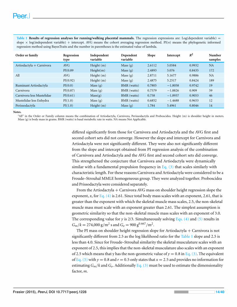
Table 1 Results of regression analyses for running/walking placental mammals. The regression expressions are: Log(dependent variable) =

slope × log(independent variable) + intercept. AVG means the cohort averaging regression method. PI(n) means the phylogenetic informedregression method using BayesTraits and the number in parentheses is the estimated value of lambda.

Order or family Regressiontype

Independentvariable

Dependentvariable

Slope Intercept R2 Numbersamples

Artiodactyla + Carnivora AVG Height (m) Mass (g) 2.6112 5.0584 0.9932 NA

PI(0.89 Height(m) Mass (g) 2.4893 5.076 0.8435 172

All AVG Height (m) Mass (g) 2.8711 5.1677 0.9886 NA

PI(0.92) Height (m) Mass (g) 2.4875 5.2517 0.8424 189

Ruminant Artiodactyla PI(0.0) Mass (g) BMR (watts) 0.7805 −1.8058 0.9742 19

Carnivora PI(0.87) Mass (g) BMR (watts) 0.7579 −1.8826 0.909 59

Carnivora less Mustelidae PI(0.61) Mass(g) BMR (watts) 0.758 −1.8937 0.9053 46

Mustelidae less Enhydra PI(1.0) Mass (g) BMR (watts) 0.6852 −1.4688 0.9653 12

Perissodactyla PI(1.0) Height (m) Mass (g) 1.784 5.4961 0.8046 14

Notes.“All” in the Order or Family column means the combination of Artiodactyla, Carnivora, Perissodactyla and Proboscidea. Height (m) is shoulder height in meters.Mass (g) is body mass in grams. BMR (watts) is basal metabolic rate in watts. NA means Not Applicable.

differed significantly from those for Carnivora and Artiodactyla and the AVG first and

second cohort sets did not converge. However the slope and intercept for Carnivora and

Artiodactyla were not significantly different. They were also not significantly different

from the slope and intercept obtained from PI regression analysis of the combination

of Carnivora and Artiodactyla and the AVG first and second cohort sets did converge.

This strengthened the conjecture that Carnivora and Artiodactyla were dynamically

similar with a fundamental propulsion frequency in Eq. (3) that scales similarly with

characteristic length. For these reasons Carnivora and Artiodactyla were considered to be a

Froude–Strouhal MMLE homogeneous group. They were analyzed together. Proboscidea

and Prissodactyla were considered separately.

From the Artiodactyla + Carnivora AVG mass on shoulder height regression slope the

exponent, x, for Eq. (4) is 2.61. Since total body mass scales with an exponent, 2.61, that is

greater than the exponent with which the skeletal muscle mass scales, 2.5, the non-skeletal

muscle mass must scale with an exponent greater than 2.61. The simplest assumption is

geometric similarity so that the non-skeletal muscle mass scales with an exponent of 3.0.

The corresponding value for y is 2/3. Simultaneously solving Eqs. (4) and (5) results in

Gm/k = 274,000 g/m2 s and Go = 900 g0.667/m2.

The PI mass on shoulder height regression slope for Artiodactyla + Carnivora is not

significantly different from 2.5 as the log likelihood ratio for the Table 1 slope and 2.5 is

less than 4.0. Since for Froude–Strouhal similarity the skeletal musculature scales with an

exponent of 2.5, this implies that the non-skeletal musculature also scales with an exponent

of 2.5 which means that y has the non-geometric value of y = 0.8 in Eq. (3). The equivalent

of Eq. (5) with y = 0.8 and r = 0.5 only states that x = 2.5 and provides no information for

estimating Gm/k and Go. Additionally Eq. (3) must be used to estimate the dimensionality

factor, m.

Frasier (2015), PeerJ, DOI 10.7717/peerj.1228 14/40

Figure 2 Log body mass as a function of log shoulder height for running/walking placental mammals. Data are from Nowak (1999). The solidand dashed lines are MMLE sturdiness factor boundaries. The upper boundaries were generated with a sturdiness factor s = (3)0.5. The lowerboundaries were generated with s = (3)−0.5. The solid boundary lines are for Froude–Strouhal dynamic similarity. The black solid lines are fory = 2/3. The colored solid lines are for y = 0.8. The dashed boundary lines are for geometric similarity. The colored boundary lines, the geometricsimilarity boundary lines and the Perissodactyla and Proboscidea mass, shoulder height data have been added to the artiodactyl and carnivoran datadisplayed in Fig. 1. For Artiodactyla and Carnivora R2

M = 0.9997 with respect to the solid black boundaries and R2M = 0.9992 with respect to the

colored boundaries. For Perissodactyla and Proboscidea R2M = 1.0 with respect to the geometric similarity boundaries. Perissodactyls are marked

with solid rectangles. Proboscideans are marked with solid diamonds. Aritiodactyla data are marked with open squares. Carnivora data are markedwith open triangles. Crossed Xes mark Hippopotamus amphibious. Xes mark domestic cattle.

Gm/k should not change if y changes. Using the previously established values of

Gm/k and Go with y = 0.8 in Eq. (3) results with a value for the dimensionality factor

of m = 4.425 g0.133.

The new values for Gm/k and Go are less than the values computed in the original paper.

The 163 samples in the original paper included two proboscideans and 11 perissodactyls

whereas the 310 samples in the present paper were entirely of Artiodactyla or Carnivora.

Figure 2 shows the MMLE mass as a function of shoulder height sturdiness factor

boundaries for simultaneous Froude–Strouhal dynamic similarity as computed by Eq. (3)

evaluated with the new values for Gm/k and Go for both y = 2/3 and for y = 0.8. The data

spans this full range of sturdiness factor for both values of y. The boundaries are hardly

distinguishable for the two y values.

Frasier (2015), PeerJ, DOI 10.7717/peerj.1228 15/40

The relationship between mass and shoulder height for Perissodactyla and Proboscidea

may be better explained by geometric similarity with a fundamental frequency of 1.4 m/s

divided by shoulder height (see Article S1).

There are doubts that ruminant artiodactyls can meet the criteria for measuring BMR

(McNab, 1997; White & Seymour, 2003). All but one of the artiodactyl samples were

ruminants. For these reasons the BMR and mass data for ruminant Artiodactyla and

Carnivora were analyzed separately. Ruminant inability to achieve a post absorptive state

should not affect the relationship between body mass and shoulder height.

There is a major composition difference between the mass and shoulder height data and

the BMR and mass data for Carnivora. Mustelidae compose only about 1% of the mass

and shoulder height data whereas they compose over 20% of the BMR and mass data. For

this reason the mustelid data was separated from the rest of the Carnivora data as shown in

Table 1.

Since the coefficient of determination, R2, for the AVG Artiodactyla + Carnivora mass

on shoulder height regression in Table 1 is very nearly unity, Eq. (6) can be used. With the

Gm/k and Go values just determined, Gr = 95.6 W−0.0079 watts/m2. The mass residual is

not significant as the log likelihood ratio for the exponent obtained with Eq. (6) and the

exponent in Table 1 is essentially 0.

Using the Carnivora less Mustelidae PI mass regressed on length and the PI BMR

regressed on mass relationships in Table 1 results with Gr = 94.5 watts/m2.

A middle value of Gr = 95 watts/m2 was used to generate the MMLE sturdiness factor

boundaries in Fig. 3. As discussed in the summary of the derivation of the MMLE equa-

tions, this value of Gr should be the basic value for all non-ruminant placental mammals.

Similarly, values for GrR for ruminant artiodactyls of 138 watts/m2 and 144 watts/m2

are obtained. GrR = 138 watts/m2 was used to generate the MMLE sturdiness factor

boundaries in Fig. 3.

The difference between slopes when regressing BMR on body mass for ruminant

artiodactyls and carnivorans excluding mustelids (Table 1) are not significant as the log

likelihood ratio is 2.8. However the difference between the intercepts is significant as

the log likelihood ratio is greater than 4.0. The significantly different intercepts support

separating ruminant Artiodactyla and Carnivora less Mustelidae for BMR analyses.

An increased mitochondrion capability quotient is not the reason that GrR is greater

than Gr. By Eq. (3) a greater mitochondrion capability quotient would result in a less

massive animal for the same characteristic length. Figure 2 shows that both Artiodactyla

and Carnivora have similar masses at the same characteristic length and their PI mass

regressed on characteristic length slopes are not significantly different. The difference

between GrR and Gr is more likely the result of sustained digestive activity by ruminant

Artiodactyla (McNab, 1997; White & Seymour, 2003).

Figure 3 shows the MMLE BMR as a function of body mass sturdiness factor boundaries

for Froude–Strouhal similarity evaluated with the new values for Gr and GrR. The

difference between the y = 2/3 and y = 0.8 slopes is significant as the log likelihood ratio is

5.9. In terms of R2M the differences are barely distinguishable.

Frasier (2015), PeerJ, DOI 10.7717/peerj.1228 16/40

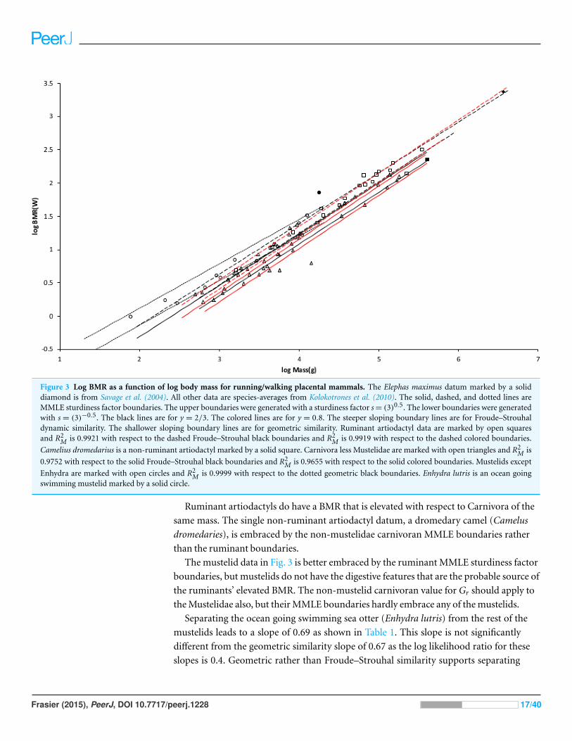
Figure 3 Log BMR as a function of log body mass for running/walking placental mammals. The Elephas maximus datum marked by a soliddiamond is from Savage et al. (2004). All other data are species-averages from Kolokotrones et al. (2010). The solid, dashed, and dotted lines areMMLE sturdiness factor boundaries. The upper boundaries were generated with a sturdiness factor s = (3)0.5. The lower boundaries were generatedwith s = (3)−0.5. The black lines are for y = 2/3. The colored lines are for y = 0.8. The steeper sloping boundary lines are for Froude–Strouhaldynamic similarity. The shallower sloping boundary lines are for geometric similarity. Ruminant artiodactyl data are marked by open squaresand R2

M is 0.9921 with respect to the dashed Froude–Strouhal black boundaries and R2M is 0.9919 with respect to the dashed colored boundaries.

Camelius dromedarius is a non-ruminant artiodactyl marked by a solid square. Carnivora less Mustelidae are marked with open triangles and R2M is

0.9752 with respect to the solid Froude–Strouhal black boundaries and R2M is 0.9655 with respect to the solid colored boundaries. Mustelids except

Enhydra are marked with open circles and R2M is 0.9999 with respect to the dotted geometric black boundaries. Enhydra lutris is an ocean going

swimming mustelid marked by a solid circle.

Ruminant artiodactyls do have a BMR that is elevated with respect to Carnivora of the

same mass. The single non-ruminant artiodactyl datum, a dromedary camel (Camelus

dromedaries), is embraced by the non-mustelidae carnivoran MMLE boundaries rather

than the ruminant boundaries.

The mustelid data in Fig. 3 is better embraced by the ruminant MMLE sturdiness factor

boundaries, but mustelids do not have the digestive features that are the probable source of

the ruminants’ elevated BMR. The non-mustelid carnivoran value for Gr should apply to

the Mustelidae also, but their MMLE boundaries hardly embrace any of the mustelids.

Separating the ocean going swimming sea otter (Enhydra lutris) from the rest of the

mustelids leads to a slope of 0.69 as shown in Table 1. This slope is not significantly

different from the geometric similarity slope of 0.67 as the log likelihood ratio for these

slopes is 0.4. Geometric rather than Froude–Strouhal similarity supports separating

Frasier (2015), PeerJ, DOI 10.7717/peerj.1228 17/40

Mustelidae from the rest of Carnivora for BMR analyses. Equation (3) with y = 2/3

and a geometric similarity fundamental frequency of 1.4 (m/s)/l and Eq. (2) are the

MMLE equations for relating BMR to body mass for geometric similarity. Of the constant

parameters in these equations, values applicable to Mustelidae for Gm, Go, and Gr have

been established. The MMLE parameters that could be adjusted to account for the

Mustelidae BMR deviation are the fundamental propulsion frequency constant, c, the

mitochondrion capability quotient, e and the dynamic similarity constant, k. Because

many Mustelidae combine swimming with terrestrial locomotion it is possible that

their skeletal musculature may not be dynamically similar to other Carnivora and the

constant k may be different from a value of 1.0. However, by Eq. (3), k and c cannot be

separated without additional information. The product kc and e were varied to obtain the

mustelid’s geometric similarity MMLE sturdiness factor boundaries shown in Fig. 3. Using

kc = 1.4 m/s as was done for Proboscidea and Perissodactyla required a mitochondrion

capability quotient at least 170% of that applicable to other Carnivora. That a mustelid

mitochondrion would be this much more powerful than other carnivoran mitochondria

is difficult to believe. Using a value of kc twice as large as that used for Perissodactyla and

Proboscidea reduced the required mitochondrion capability quotient to 130% of that

for other carnivorans. An implication would be that more powerful mitochondria allow

mustelids to move their limbs twice as fast as other placental mammals in performing

routine locomotion tasks.

Coverage, R, is the fraction of samples that fall between the MMLE sturdiness

boundaries. Separating the Mustelidae from the rest of the Carnivora increased R for

the entire Carnivora order from about 0.44 to 0.53 for y = 2/3 and from about 0.39 to 0.49

for y = 0.8. Although coverage is somewhat sparse, many of the samples lie close to the

MMLE sturdiness boundaries as the greater R2M values indicate.

For the groups for which it could be determined, Table 2 shows which skeletal

musculature and which non-skeletal musculature similarity models are applicable to which

MMLE homogeneous group for the running/walking placental mammals and for other

groups that will be addressed soon.

RODENTIA RESULTSRodentia comprise about 20% of families, 39% of genera, and 43% of species of recent

mammals. Their masses range over four and a half orders of magnitude and their head

and body lengths range over one and a half orders of magnitude (Mus minutoides with a

mass of 2.5 g and head and body length of 45 mm to Hydrochaeris hydrochaeris with a mass

of 79,000 g and head and body length of 1,300 mm). Various species employ scurrying,

climbing, gliding, hopping, burrowing, swimming, running/walking, and combinations of

these as their primary means of locomotion (Nowak, 1999).

Froude similarity should apply to skeletal muscle dynamics in most Rodentia as gravity

is the main force affecting their locomotion. This should be true even for swimming as

aquatic Rodentia are mainly surface swimmers that experience significant drag through

the generation of surface waves in the wake. Drag through the generation of surface waves

Frasier (2015), PeerJ, DOI 10.7717/peerj.1228 18/40

Table 2 Similarity models applicable to MMLE homogeneous groups. The similarities are indicated bythe regression analysis results reported in Tables 1, 3, and 4. Total body mass is the sum of the masses ofthe skeletal and non-skeletal musculatures.

MMLE homogeneousgroup

Skeletal musculaturesimilarity model

Non-skeletal musculaturesimilarity model

Artiodactyla + Carnivoraless Mustelidae

Froude–Strouhal Geometrica

Artiodactyla + Carnivoraless Mustelidae (alternate)

Froude–Strouhal Non-Geometricb

Mustelidae less Enhydra Geometricc Geometric

Non-Cricetidae Rodentia Mixture of Geometricc

and Froude–StrouhalGeometric

Cricetidae Geometricc Geometric

Light bats Geometricd Geometric

Heavy bats Strouhal Geometric

Intermediate bats Mixture of Geometricd

and StrouhalGeometric

Notes.a Similarity indicated by the results of the cohort averaging regression method (AVG) results.b Similarity indicated by the results of the phylogenetic informed regression method (PI) results.c Compatible with Froude dynamic similarity.d Compatible with Strouhal dynamic similarity.

in the wake is the classic situation to which Froude similarity applies (Newman, 1977).

What should govern the dynamics of burrowing is not clear, but as will be seen Froude

similarity seems to work. The mass regressed on head and body length slope for both PI

and AVG regressions for all families of Rodentia trends toward the geometric slope of

3.0. The combination of all families except Cricetidae trend toward an intermediate slope

between the Froude–Strouhal slope of around 2.55 for mammals the size of Rodentia and

the geometric slope. Cricetidae have an AVG mass regressed on length slope nearer the

geometric similarity slope and the PI slope exceeds geometric similarity. Cricetidae also

have a PI BMR regressed on mass slope that is not significantly different than the slope for

geometric similarity as the log likelihood ratio for the slopes is 4.0.

Besides appearing to be more geometrically similar, cricetids tend to have a higher

BMR when compared to non-cricetids of the same mass. For these reasons Cricetidae were

analyzed separate from all the other families of Rodentia.

The slope values for mass regressed on head and body mass in Table 3 for both PI and

AVG regressions are very different from the value of 2.5 obtained for y = 0.8 for Artio-

dactyla + Carnivora. They indicate either geometric similarity with y = 2/3 or a mixture

of geometric similarity and Froude–Strouhal similarity with y = 2/3. For non-Cricetidae,

the PI regression slope is not significantly different from the AVG slope as the log likelihood

ratio for the two slopes is less than 4.0. For these reasons the geometric similarity value for

the non-skeletal muscle exponent of y = 2/3 is used in Eq. (3) for Rodentia.

The skeletal musculature and non-skeletal musculature similarity models that are

applicable to the rodent MMLE homogeneous groups are shown in Table 2.

Frasier (2015), PeerJ, DOI 10.7717/peerj.1228 19/40

Table 3 Results of regression analyses for rodentia. The regression expressions are: Log(dependent variable) = slope X log(independent variable)+ intercept.

Family Regressiontype

Independentvariable

Dependentvariable

Slope Intercept R2 Numbersamples

All Rodentia PI(0.62) Mass (g) BMR (watts) 0.7231 −1.7198 0.8968 267

PI(0.0) Length (mm) Mass (g) 2.9482 −4.3637 0.9571 105

AVG Length (mm) Mass (g) 2.8692 −4.1497 0.9956 NA

Non- PI(0.44) Mass (g) BMR (watts) 0.7399 −1.7685 0.9192 176

Cricetidae PI(0.0) Length (mm) Mass (g) 2.9079 −4.2548 0.9571 78

AVG Length (mm) Mass (g) 2.8564 −4.1124 0.9939 NA

Cricetidae PI(0.55) Mass (g) BMR (watts) 0.6597 −1.5408 0.8497 91

PI(0.0) Length (mm) Mass (g) 3.4061 −5.3367 0.9395 27

AVG Length (mm) Mass (g) 2.9531 −4.3561 0.9908 NA

Notes.PI(n) means the phylogenetic informed regression method using BayesTraits and the number in parentheses is the estimated value of lambda. AVG means the cohortaveraging regression method. Length (mm) is head and body length in millimeters. Mass (g) is body mass in grams. NA means Not Applicable.

Figure 4 Log body mass as a function of log head and body length for non-cricetid rodents. Dataare from Nowak (1999). The solid and dashed lines are MMLE sturdiness factor boundaries. The upperboundaries were generated with a sturdiness factor s = (3)0.5. The lower boundaries were generated withs = (3)−0.5. The shallower sloping solid boundary lines are for Froude–Strouhal similarity. The steepersloping dashed boundary lines are for geometric similarity. Non-cricetid rodents are marked by opencircles. R2

M = 0.9995 with respect to both sets of boundaries.

Given the available data, linearly relating head and body length to characteristic length

was tried. The characteristic length for Rodentia was assumed to be a constant fraction

of head and body length. The fraction’s value was estimated by equating the combined

Frasier (2015), PeerJ, DOI 10.7717/peerj.1228 20/40

Figure 5 Log BMR as a function of log body mass for non-cricetid rodents. Data are from Kolokotroneset al. (2010). The solid and dashed lines are MMLE sturdiness factor boundaries. The upper boundarieswere generated with a sturdiness factor s = (3)0.5. The lower boundaries were generated with s = (3)−0.5.The steeper sloping solid boundary lines are for Froude–Strouhal similarity. The shallower sloping dashedboundary lines are for geometric similarity. The species-averaged non-Cricetidae Rodentia are markedby open circles. R2

M = 0.9966 with respect to both sets of boundaries.

Artiodactyla and Carnivora mass regressed on length expression to the all families of

Rodentia mass regressed on head and body length for the range of lengths for Rodentia.

This results in a fraction that is within the range 0.4 to 0.62 using the PI regression

relationship and 0.43 to 0.61 using the AVG relationship. A value of 0.5 was considered

to be a reasonable working estimate for this characteristic length scaling fraction.

The characteristic length scaling fraction adds an additional parameter to the number

that MMLE uses to predict the absolute values of body mass and BMR.

The fundamental locomotion frequency for geometric similarity is a constant divided

by the characteristic length. The value of 1.4 m/s for the constant that worked well for

Perissodactyla and Proboscidea was also used as the constant for Rodentia.

Figure 4 shows the MMLE mass as a function of head and body length sturdiness factor

boundaries for Froude–Strouhal dynamic similarity and geometric similarity evaluated

with the same constants that were used for running/walking mammals and a characteristic

length scaling factor of 0.5.

Figure 5 shows the MMLE BMR as a function of body mass sturdiness factor boundaries

for the two similarity regimes evaluated with the same constants that were used for

non-Mustelidae Carnivora and a characteristic length scaling factor of 0.5.

Frasier (2015), PeerJ, DOI 10.7717/peerj.1228 21/40

Figure 6 Log body mass as a function of log head and body length for Cricetidae. The data are fromNowak (1999). The dashed lines are MMLE sturdiness factor boundaries. The upper boundary wasgenerated with a sturdiness factor s = (3)0.5. The lower boundary was generated with s = (3)−0.5. Theboundary lines are for geometric similarity. Cricetids are marked by open diamonds. R2

M = 1.0.

As with Mustelidae that have a greater BMR at the same body mass than do other

Carnivora, a greater mitochondrion capability quotient would most straight forwardly

result in a greater BMR for Cricetidae with the same masses as other Rodentia. Varying it

until a maximum value of R2M was achieved for both mass as a function of length and BMR

as a function of mass resulted in a mitochondrion capability quotient of 1.2. Figure 6 shows

the MMLE mass as a function of head and body length sturdiness factor boundaries for

geometric similarity evaluated with this mitochondrion capability quotient value. Figure 7

shows the MMLE BMR as a function of body mass sturdiness factor boundaries.

A mitochondrion capability quotient of 1.2 as an explanation of why Cricetidae have an

elevated BMR with respect to other Rodentia is considerably more palatable than the value

of this parameter needed to explain the elevated BMR of Mustelidae with respect to other

Carnivora.

BATS (THE ORDER CHIROPTERA) RESULTSBats are second only to rodents in the number of species among mammals. Bats comprise

about 12% of families, 16% of genera, and 20% of species of recent Mammals. Their

masses range over three orders of magnitude from Craseonycteris thonglongyai and

Tylonycteris pachypus with masses as small as 2 g to Pteropus giganteus with a mass of as

much as 1,600 g (Nowak, 1999).

Frasier (2015), PeerJ, DOI 10.7717/peerj.1228 22/40

Figure 7 Log BMR as a function of log body mass for Cricetidae. The data are from Kolokotroneset al. (2010). The dashed lines are MMLE sturdiness factor boundaries. The upper boundary wasgenerated with a sturdiness factor s = (3)0.5. The lower boundary was generated with s = (3)−0.5. Theboundary lines are for geometric similarity. Cricetid species-averaged BMR, mass data are marked byopen diamonds. R2

M = 0.9913.

Bats primary means of locomotion is flying by flapping very flexible membranous

wings controlled by multi-jointed fingers (Muijres et al., 2011). Unlike birds, bats use their

hind limbs as well as their fore limbs to flap their wings (Norberg, 1981). Bats experience

daily and seasonal fluctuations in body mass which they accommodate by changes in

wing kinematics that vary among individuals (Iriarte-Diaz et al., 2012). To analyze the

applicability of MMLE theory to bats, a characteristic length and a fundamental propulsion

frequency related to very complicated flapping wing flight needed to be identified. The

characteristic length should be related to wing dimensions. Norberg (1981) found that

forearm length scaled with body mass with about the same exponent as wing span. Given

the options available with the Nowak (1999) data, it was assumed that forearm length is

linearly related to characteristic length. A possible complication that is avoided by this

assumption is that full wing dimensions, such as wing span, in a flying bat may vary with

flight mode and speed and may be different than those measured from specimens stretched

out flat on a horizontal surface (Riskin et al., 2010).

Norberg & Rayner (1987) found that geometric similarity applied for most bat wing

dimensions with some exceptions. More recent work suggests that wing bone lengths are

also geometrically similar with respect to body mass in different sized bats (Norberg &

Norberg, 2012).

Frasier (2015), PeerJ, DOI 10.7717/peerj.1228 23/40

Table 4 Results of bat regression analyses. The regression expressions are: log(dependent variable) = slope × log(independent variable) +

intercept.

Order orfamily

Regressiontype

Independentvariable

Dependentvariable

Slope Intercept R2 Numbersamples

All bats PI(0.93) Length (mm) Mass (g) 2.6668 −3.3211 0.8507 176

AVG Length (mm) Mass (g) 2.7718 −3.3628 0.9924 NA

Megachiroptera PI(0.33) Length (mm) Mass (g) 2.8628 −3.4933 0.9749 40

AVG Length (mm) Mass (g) 2.7335 −3.2632 0.9978 NA

Microchiroptera PI(0.93) Length (mm) Mass (g) 2.515 −3.1025 0.7522 136

AVG Length (mm) Mass (g) 2.5292 −2.9844 0.9928 NA

Heavy bats PI(0.79) Length (mm) Mass (g) 2.7595 −3.3252 0.922 86

AVG Length (mm) Mass (g) 2.7233 −3.2329 0.9937 NA

Light bats PI(0.0) Length (mm) Mass (g) 3.28 −4.4926 0.8781 29

AVG Length (mm) Mass (g) 2.9878 −3.9552 0.9743 NA

All bats PI(0.83) Mass (g) BMR (watts) 0.8111 −1.9063 0.8784 84

Megachiroptera PI(0.56) Mass (g) BMR (watts) 0.8581 −2.0161 0.9279 21

Microchiroptera PI(1.07) Mass (g) BMR (watts) 0.7459 −1.8247 0.991 63

Heavy bats PI(0.89) Mass (g) BMR (watts) 0.8225 −1.9166 0.8887 51

Light Batsa PI(0.0) Mass (g) BMR (watts) 0.7015 −1.8048 0.8154 17

Notes.a Data available for only 4 of the 8 families comprising light bats.

PI(n) means the phylogenetic informed regression method using BayesTraits and the number in parentheses is the estimated value of lambda. AVG means the cohortaveraging regression method. Length (mm) is forearm length in millimeters. Mass (g) is body mass in grams. NA means Not Applicable.

The order Chiroptera is divided into two suborders: the Megachiroptera consisting

of the single family Peteropodidae and the Microchiroptera consisting of all other bats

(Nowak, 1999). Table 4 shows the regression analysis results obtained with forearm length

data and BMR data for all bats and for the two suborders considered separately. The

geometric similarity non-skeletal muscle mass exponent value of y = 2/3 is consistent with

both the PI and AVG all bats results and the Megachiroptera results. The non-geometric

value of y = 0.8 is consistent with both PI and AVG results for Microchiroptera.

Figure 8 offers an alternative partitioning for bats in which the bat families have been

divided into three groups: ‘heavy’ bats, ‘light’ bats and ‘intermediate’ bats. At the same

forearm length members of families composing the heavy bats are mostly more massive

than those of the families composing the light bats. Intermediate bats span both the heavy

and light mass regimes. The families composing the three groups are given in the caption of

Fig. 8.

For the AVG regression of log mass on log forearm length the slope for light bats is

very nearly the 3.0 expected for geometric similarity and the slope of the PI regression

relationship is not significantly different from 3.0 as the log likelihood ratio is only 2.7.

Light bats appear to be geometrically similar.

Pteropodidae and Phyllostomidae comprise the heavy bats. The Pteropodidae contain

the Old World frugivores and the Phyllostomidae contain the New World frugivores.

While both families have species with other diets, the frugivores have wings adapted to

commuting long distances from roost to feeding areas (Norberg & Rayner, 1987). The

Frasier (2015), PeerJ, DOI 10.7717/peerj.1228 24/40

Figure 8 Log body mass as a function of log forearm length for bats. At the same forearm length individuals from families composing the ‘heavy’bats marked with Xes are mostly more massive than those from the families composing the ‘light’ bats marked with open rectangles. ‘Intermediate’bats marked with open circles span both the heavy and light mass regimes. The families Pteropodidae and Phyllostomidae comprise the heavy bats.The families Emballonuridae, Craseonycteridae, Rhinopomatidae, Rhinolophoidea, Mormoopidae, Noctilionidae, Furipteridae and Hipposideridaecomprise the light bats. The families Nycteridae, Megadermatidae, Vespertilionoidae, Thyropteridae, Myzopodidae, Natalidae, Mystacinidae, andMolossidae comprise the intermediate bats.

Frasier (2015), PeerJ, DOI 10.7717/peerj.1228 25/40

relationships between wing dimensions and body mass should be similar for the frugivore

members of the two families.

The fundamental propulsion frequency for bats should be related to the wing flapping

frequency. A bat’s wing flapping frequency increases slightly with air speed at lower speeds.

It becomes almost independent of speed at higher speeds. The speed at which the transition

occurs is the preferred speed (Bullen & McKenzie, 2002). The wing flapping frequency at

this preferred speed should be proportional to the fundamental propulsion frequency.

Animals that fly by flapping wings operate in a narrow range of Strouhal numbers

in cruising flight (Taylor, Nudds & Thomas, 2003). Strouhal number does not change

significantly for Pteropodidae (Riskin et al., 2010). It appears to be an accurate predictor of

wingbeat frequency for birds (Nudds, Taylor & Thomas, 2004). Strouhal dynamic similarity

should apply to bats.

For bats Strouhal number = (wingbeat frequency) × (wingbeat amplitude)/(air speed).

Wingbeat amplitude is the vertical distance the wing tip travels during a stroke. Under

Strouhal dynamic similarity the wingbeat amplitude should be proportional to the MMLE

characteristic length. It was assumed that wingbeat amplitude characteristic length is a

fraction of forearm length for bats. Further analysis involving maximization of R2M for light

bat BMR resulted with characteristic length = 0.61 of forearm length, kc = 0.625 m/s and

R2M = 0.9984 (see Article S1).

Strouhal dynamic similarity is consistent with geometric similarity. Since the funda-

mental propulsion frequency under geometric similarity is proportional to the inverse of

the characteristic length, simultaneous geometric and Strouhal similarity imply that the

preferred flight speed is approximately constant.

Since R2 is nearly unity for the AVG regression relationship of Table 4, Eq. (6) should

apply. The log likelihood for the resulting exponent, 2/x = 0.6694 could not be calculated

using BayesTraits. Thus the significance of its difference from the BMR regressed on mass

exponent in Table 4 could not be determined. It is noted that length and mass data was

available to estimate x for all families composing the light bats group but BMR and mass

data to estimate the BMR regressed on mass exponent was available for only four of the

eight families.

Figure 9 shows the MMLE BMR as a function of body mass boundaries for geometric

similarity for light bats evaluated with these estimates.

A methodology similar to that used for light bats was used to establish the characteristic

length scaling fraction and fundamental propulsion frequency constant for heavy bats. By

the heavy bat regression relationships of Table 4, heavy bats are not geometrically similar.

Since heavy bats are not geometrically similar the exponent, r, in the relationship between

fundamental propulsion frequency and characteristic length in Eqs. (3) and (5) also had

to be established. The results using the Table 4 AVG relationships were characteristic

length = 0.92 forearm length, r = 0.68, kc = 3.22 m0.68/s and R2M for BMR = 0.9828.

The results using the PI relationships were characteristic length = 0.86 forearm length,

r = 0.73, kc = 2.59 m0.73/s, and R2M for BMR = 0.9918. In terms of R2

M the PI and AVG

results are nearly indistinguishable (see Article S1).

Frasier (2015), PeerJ, DOI 10.7717/peerj.1228 26/40

Figure 9 Log BMR as a function of log body mass for heavy and light bats. The solid and dashed linesare the MMLE sturdiness factor boundaries. The upper boundaries were generated with a sturdiness fac-tor s = (3)0.5. The lower boundaries were generated with s = (3)−0.5. The steeper sloping solid boundarylines are for heavy bat Strouhal dynamic similarity. The shallower sloping dashed boundary lines arefor light bat geometric similarity. R2

M = 0.9828 for heavy bats with respect to the Strouhal boundaries.

R2M = 0.9984 for light bats with respect to the geometric boundaries. Heavy bat species-averaged data are

marked with Xes. Light bats species-averaged data are marked with open rectangles. Data was availablefor only four of the eight families comprising the light bats.

Since R2 is nearly unity for the heavy bat AVG mass regressed on length relationship in

Table 4, Eq. (6) should apply. The difference between the resulting exponent, 2/x = 0.7344

and the PI BMR regressed on mass exponent in Table 4 is borderline significant as the log

likelihood ratio is 4.1.

Figure 9 also shows the MMLE log BMR as a function of log body mass MMLE

sturdiness factor boundaries for heavy bats evaluated with these estimates.

Figure 10 shows the MMLE log body mass as a function of log forearm length MMLE

sturdiness factor boundaries for both heavy bats and geometrically similar light bats.

Figure 11 shows the MMLE log BMR as a function of log body mass MMLE sturdiness

factor boundaries for both heavy bats and light bats. Species averaged BMR and body mass

samples for intermediate bats are also shown. The data spreads over both MMLE bands as

Frasier (2015), PeerJ, DOI 10.7717/peerj.1228 27/40

Figure 10 Log body mass as a function of log forearm length for heavy and light bats. The solid anddashed lines are the MMLE sturdiness factor boundaries. The upper boundaries were generated witha sturdiness factor s = (3)0.5. The lower boundaries were generated with s = (3)−0.5. The shallowersloping solid boundary lines are for heavy bat Strouhal dynamic similarity. The steeper sloping dashedboundary lines are for light bat geometric similarity. R2

M = 1.0 for heavy bats with respect to the Strouhal

boundaries. R2M = 1.0 for light bats with respect to the geometric boundaries. Individual heavy bats are

marked with Xes. Individual light bats are marked with open rectangles.

if within the same family there are species that conform to geometric similarity and other

species that conform to heavy bat Strouhal similarity.

Figure 12 shows the MMLE log body mass as a function of log forearm length MMLE

sturdiness factor boundaries for both heavy and light bats. Body mass and forearm length

samples for intermediate bats are also shown. Intermediate bat body mass is explained

almost equally well by either the geometrically similar light bat MMLE band or the heavy

bat MMLE band as the R2M values indicate.

The light and heavy bat data in Fig. 10 does not fully occupy their respective MMLE

sturdiness factor bands. This raises the possibility that a sturdiness factor range narrower

than (3)−0.5 to (3)0.5 may apply to heavy or light bats. The intermediate bat data in

Fig. 12 more completely occupies both bands indicating that the full sturdiness factor

range is applicable. The situation may be more complicated. Each of the heavy, light and

Frasier (2015), PeerJ, DOI 10.7717/peerj.1228 28/40

Figure 11 Log BMR as a function of log body mass for intermediate bats. The solid and dashed lines arethe MMLE sturdiness factor boundaries. The upper boundaries were generated with a sturdiness factors = (3)0.5. The lower boundaries were generated with s = (3)−0.5. The steeper sloping solid boundarylines are for heavy bat Strouhal dynamic similarity. The shallower sloping dashed boundary lines arefor light bat geometric similarity. Data was available for only four of the eight families comprising theintermediate bats. R2

M = 0.9678 for intermediate bats with respect to the Strouhal boundaries. R2M =

0.9893 for intermediate bats with respect to the geometric boundaries. R2M = 0.9998 for intermediate

bats with respect to both sets of boundaries. The data are species-averaged. Megadermatidae are markedwith crossed Xes. Molossidae are marked with open triangles. Vesperstilionidae are marked with opencircles. Natalidae are marked with open squares.

intermediate bat groups contains species with different food habits. Bat wing morphology

is associated with flight behavior related to food habits. Even among the insectivores that

dominate the light and intermediate groups there are different styles of catching insects

that are associated with differing wing morphologies (Norberg & Rayner, 1987; Norberg &

Norberg, 2012). Dynamic similarity may apply at a phylogenetic level below the family.

The light-intermediate-heavy representation of bats is better supported by the data than

either the all bats representation or the Megachiroptera-Microchiroptera representation in

terms of R2M and coverage, R (see Article S1). Table 2 shows which skeletal musculature and

Frasier (2015), PeerJ, DOI 10.7717/peerj.1228 29/40

Figure 12 Log body mass as a function of log forearm length for intermediate bats. The solid anddashed lines are the MMLE sturdiness factor boundaries. The upper boundaries were generated witha sturdiness factor s = (3)0.5. The lower boundaries were generated with s = (3)−0.5. The shallowersloping solid boundary lines are for heavy bat Strouhal dynamic similarity. The steeper sloping dashedboundary lines are for geometric similarity. R2

M = 0.998 for intermediate bats with respect to the Strouhal

boundaries. R2M = 0.9981 for intermediate bats with respect to the geometric boundaries. R2

M = 0.9999for intermediate bats with respect to both sets of boundaries.

which non-skeletal musculature similarity models are applicable to the light, heavy and

intermediate bat MMLE homogeneous groups.

COMPUTATION ERRORWith a body mass and characteristic length data set such as Nowak (1999), Eq. (3) is exact

for a MMLE homogeneous group because for every datum a value for the sturdiness factor

can be found such that the body mass is exactly computed by the equation using this found

sturdiness factor and the characteristic length. With a BMR and body mass data set such

as Kolokotrones et al. (2010), Eqs. (2) and (3) are exact because for every datum a value

for the sturdiness factor and a value for the characteristic length can be found such that

the BMR is exactly computed by Eq. (2) and the body mass is exactly computed by Eq. (3)

using the found sturdiness factor value and the found characteristic length value. For the

Frasier (2015), PeerJ, DOI 10.7717/peerj.1228 30/40

same reasons, Eqs. (2) and (3) are exact with other MMLE homogeneous groups once

the non-characteristic length and non-sturdiness factor parameters that make the groups

different are determined.

The ability of MMLE to exactly compute every datum obtained from the appropriate

data set does not necessarily mean that there is no unexplained variance with MMLE

theory. Equations 2 and (3) apply simultaneously to a particular individual animal which

has particular values for body mass, BMR, and characteristic length. The author of the

present paper is unaware of a data set that reports all three of these values for individual

animals. Instead there is the data set from Nowak (1999) reporting individual body mass

and characteristic length and another data set from Kolokotrones et al. (2010) that reports

species-averaged BMR and body mass. It is unlikely that the same particular animal is

included in both data sets. There is likely to be unexplained variance with a data set that

simultaneously reports the three values of mass, BMR and length for individual animals.

The unexplained variance would be detected by the need to use one value of the sturdiness

factor in Eq. (3) to accurately compute mass and a different value in Eq. (2) to accurately

compute BMR for the same animal.

That there could be unexplained variance with a data set that reports the three values of

mass, BMR and length for individual animals is suspected because of measurement errors

and because MMLE theory as currently expressed does not account for body temperature

effects on the mitochondrion capability quotient. Body temperature has a significant effect

on BMR (Clarke, Rothery & Isaac, 2010; Kolokotrones et al., 2010).

However, as shown in Table 5, MMLE is able to predict the BMR regressed on mass

exponent obtained by PI regression analysis of BMR and mass data from the mass regressed

on length exponent obtained by AVG regression analysis of length and mass data for many

of the MMLE homogeneous groups addressed in this paper. This is a result of being able

to use Eq. (6) because R2 is nearly unity for the AVG regression analyses. This might not

be significant for the multiplicative constants in Eqs. (2) and (6) as the regression analyses

for both data sets were used to estimate the value of Gr that occurs in both equations. But

the exponents are independent of the multiplicative constants. These considerations argue

that MMLE may be able to simultaneously compute an individual animal’s mass and BMR

given its characteristic length and sturdiness factor; or looked at another way, it may be

possible to find sturdiness factors so that MMLE can compute every datum from a data set

that simultaneously reports individual animals’ mass, characteristic length and BMR.

DISCUSSION10 parameters were theoretically derived to compute BMR and body mass with MMLE

(11 parameters if a characteristic length scaling factor is needed). The parameters emerged

from the theoretical derivation of MMLE from the principles of physics and physiology

that were being considered. 10 parameters are only one more than the number of factors

that McNab (2008) found influenced mammal BMR; and it is less than the over 22

parameters needed to best describe the overall mass and temperature dependence of BMR

by the White, Frappell & Chown (2012) information-theoretic analysis. While that analysis

Frasier (2015), PeerJ, DOI 10.7717/peerj.1228 31/40

Table 5 Comparison of the theoretical value of the exponent, b, with the value obtained by PI re-gression analysis for the equation BMR = aWb for MMLE homogeneous groups. The exponents fromPI regression analyses, b, are the slope values reported in Tables 1, 3 and 4 for the PI regression typewith independent variable Mass (g) and dependent variable BMR (watts). The theoretical exponent iseither (1) the value assuming geometric similarity or (2) the Eq. (6) value, 2/x, where x is the slopevalue reported in Tables 1, 3 or 4 for the AVG regression type with independent variable Height (m) orLength (mm) and dependent variable Mass (g). The values for x were obtained by analyses of data fromNowak (1999) by the cohort averaging regression method (AVG). The PI regression analysis exponentswere obtained by Phylogenetically Informed (PI) regression analyses of Kolokotrones et al. (2010) datausing BayesTraits. A log likelihood ratio less than 4.0 means that an exponent from the PI regressionanalysis column is not significantly different from the corresponding exponent from the theoreticalexponent column (Pagel, 1999).

MMLE homogeneousgroup

Exponentfrom PIregressionanalysis, b

Theoreticalexponent

Loglikelihoodratio

Significantdifference?

Carnivora less Mustelidae 0.758 0.7651(2) 0.1 N

Ruminant artiodactyls 0.7805 0.7651(2) 2.8 N

Mustelidae less Enhydra 0.6852 0.6667(1) 0.4 N

Cricetidae Rodentia 0.6597 0.6773(2) 17.8 Y

Cricetidae Rodentia 0.6597 0.6667(1) 4.0 N

Heavy bats 0.8225 0.7344(2) 4.1 Y/N

Light bats 0.7015 0.6694(2) NC NC

Notes.N means “no”, Y means “yes” and Y/N means borderline. NC means that a log likelihood ratio could not be calculatedfor the Light bats group.

did include insects, spiders, protists and prokaryotes as well as vertebrates, it and McNab’s

findings do indicate that needing a large number of parameters to predict the absolute

value of a vertebrate’s body mass and BMR should not be surprising. Even describing the

relationships between BMR and body mass, W, and a skeletal dimension, l, for a collection

of animals with the simple relationships BMR = aWb and W = dlx requires at least five

parameters and as many as six if BMR and length data are not for the same individual ani-

mals. Simplicity is not necessarily better than complexity (White, Frappell & Chown, 2012).

Finding new values for the fundamental propulsion frequency constant, c, the

mitochondrion capability quotient, e and the dynamic similarity constant, k to reconcile

Cricetidae with the rest of Rodentia and to reconcile Mustelidae with the rest of Carnivora

or the division of bats into three new groups could appear to be forcing MMLE to fit the

data. However these instances are legitimate uses of the degrees of freedom available with

MMLE to explain differences that were observed in the data.

The results of regression analyses were used to estimate numerical values for the param-

eters. Phylogenetic informed (PI) regression analysis was performed on taxon-averaged

data using BayesTraits. AVG regression analysis was performed on individual body mass,

characteristic length data. AVG regression is unique to MMLE theory. Parameter numerical

values estimated from results obtained with the two regression techniques did differ. In

terms of the two MMLE measures of effectiveness, R2M and R, body masses computed by

Frasier (2015), PeerJ, DOI 10.7717/peerj.1228 32/40

Eq. (3) and BMR computed by Eq. (2) are nearly indistinguishable when using parameters

estimated from the results of either technique.

The values for the constants Gm, Go and Gr were derived from running/walking

placental mammal data. Since the values obtained in the present paper differ from the

values obtained with the data that was available over a quarter of a century ago, it would

not be surprising if the values should be refined again in the future.

Using Eq. (3) the ratio of volume active tissue mass to total body mass for geometrically

similar running/walking placental mammals is calculated to vary from 81% for sturdy

animals to 93% for gracile animals. For Strouhal–Froude dynamically similar animals the

ratio varies from 87% for small sturdy animals to 91% for small gracile animals; and for

large animals it varies from 61% for sturdy animals to 74% for gracile animals. The ratio

of muscle to total body mass appears to vary between 21% and 61% for mammals (Much-

linski, Snodgrass & Terranova, 2012). The MMLE volume active tissues appear to be about

twice as massive as the skeletal musculature. This leads to the possibility that inclusion of a

third type of tissue in the MMLE representation of the vertebrate body may be warranted.

The third tissue type would include everything that is not skeletal muscle, liver, heart, kid-

neys, and brain. It would have few mitochondria so that it would contribute little to BMR.

Three types of dynamic similarity were encountered for the skeletal musculature of the

placental mammals examined in the present paper: Froude similarity, Strouhal similarity

and simultaneous Froude and Strouhal similarity. Geometric similarity is compatible with

either Froude or Strouhal similarity. It is not compatible with simultaneous Froude and

Strouhal similarity. The type of dynamic similarity that governs the morphology of an

animal’s skeletal musculature seems to correlate with a phylogenetic level that may be as

low as the species.

Compared with the original paper (Frasier, 1984), the present paper makes important

modifications to MMLE theory. The fundamental propulsion frequency is generalized to

f = c/lr where c is the fundamental propulsion frequency constant, l is the characteristic

length and r is the fundamental propulsion frequency exponent. This generalization allows

the different types of dynamic similarity to be explicitly addressed by Eq. (3). The mass

of the non-skeletal musculature is also generalized to allow non-geometrically similar

topologies to be explicitly addressed by Eq. (3). Ordinary Least Squares regression analyses

are replaced by PI analyses in the present paper. The present paper estimates new numer-

ical values for the parameters occurring in Eqs. (2) and (3) by analysis of data that was

unavailable when the original paper was written. The present paper furthermore extends

the demonstration of MMLE theory’s ability to exactly compute body mass and BMR for

individual animals from about 9% of placental mammals to about 72% by adding Rodentia

and bats to running/walking Artiodactyla, Carnivora, Perissodactyla and Proboscidea.

Carnivora with body masses less than about 2,000 g were not included in the body mass

as a function of characteristic length analysis of running/walking placental mammals. They

were not included because their shoulder heights are not given in Nowak (1999). However

head and body lengths are given. The methodology of using a scaling fraction to translate

Frasier (2015), PeerJ, DOI 10.7717/peerj.1228 33/40

heady and body length to characteristic length as was done for Rodentia may also work for

small Carnivora.

MMLE’s ability to compute BMR and body mass for the mammal orders that were

not included in the present paper should be examined. A complication is that from an

examination of Kolokotrones et al. (2010) it appears that BMR data are scarce except for the

orders Primates, Soricomorpha, Dasyuromorpha and Diprotodontia.

MMLE should apply to all vertebrates. The original paper tried to address birds but that

analysis now appears to be simplistic. The analysis should be performed again with recent

data and the expanded version of MMLE presented in the present paper.

The sturdiness factor adds additional information about the composition of an

animal’s body that is missing from relationships of the form aWb. Consideration of body

composition can reduce unexplained variance even for relationships that express BMR as a

function of body mass (Raichlen et al., 2010; Muller et al., 2011).

The Raichlen, Pontzer & Shapiro (2013) finding that hip joint to limb center of mass

length is a better length for establishing the pendulum frequency for Froude–Strouhal

similar animals may affect the concept of the sturdiness factor. Sturdier animals have

stouter limbs which should cause the limb’s center of mass to be further from the hip

joint and thereby increase the characteristic length. For this reason it is possible that the

sturdiness factor may be, in part, a scaling factor for converting characteristic length

surrogates such as shoulder height into hip joint to limb center of mass lengths.

MMLE theory as currently expressed does not account for body temperature effects on

the mitochondrion capability quotient. Body temperature has a significant effect on BMR

(Clarke, Rothery & Isaac, 2010; Kolokotrones et al., 2010). The extent to which the inclusion

of temperature effects on the mitochondrion capability quotient would improve MMLE’s

accuracy awaits a complete data set reporting body temperature as well as mass, BMR and

length for individual animals. In the meantime, the body temperature data in Kolokotrones

et al. (2010) could be used to examine the extent to which inclusion of temperature in

Eq. (3) would narrow the sturdiness factor range needed to bound the Kolokotrones et al.

(2010) BMR and mass data and the Nowak (1999) mass and length data.

While the mitochondrion capability quotient used in Eq. (3) should have approximately

the same value for all animals with the same body temperature in the same phylogenetic

group, genetic variation could cause it to vary among individuals or populations in the

same species. Variation of the mitochondrion capability coefficient together with variation

of the sturdiness factor would cause mass-independent variation in the BMR of animals

like that recently addressed by White & Kearney (2013).

MMLE was derived for fit animals surviving in the wild. Captivity, domestication,

inactivity and sickness could cause an animal’s body mass or BMR to be different from

that predicted by MMLE. In particular, muscle or mitochondrion atrophy due to decreased

activity with respect to that experienced in the wild would likely cause a difference.

Frasier (2015), PeerJ, DOI 10.7717/peerj.1228 34/40

CONCLUSIONThe purpose of this paper was to use modern resources to revisit MMLE theory and test

its ability to compute the absolute values of BMR and body mass for individual animals.

With some modifications to the theory as originally formulated (Frasier, 1984) MMLE

can exactly compute every individual BMR given body mass datum and every individual

body mass given characteristic length datum for the recent data sets that were examined

(Nowak, 1999; Kolokotrones et al., 2010) and for the mammal orders examined. MMLE

deterministically computes the absolute value of BMR and body mass for individual

animals rather than a statistical best fit average value for a collection of individuals from a

single species which is the usual methodology used by other examinations of these topics

(White & Kearney, 2014). The examined mammal orders include over two thirds of recent

mammal species.

Determining if MMLE can simultaneously exactly compute an individual animal’s

BMR and body mass given its characteristic length awaits a data set that simultaneously

reports all three values for individual animals. However MMLE’s ability to predict the BMR

regressed on mass exponent obtained by PI regression analysis of BMR and mass data from

the mass regressed on length exponent obtained by AVG regression analysis of length and

mass data for many of the MMLE homogeneous groups addressed in this paper argues that

accurate simultaneous prediction of mass and BMR for the same animal may be possible.

ACKNOWLEDGEMENTSI thank Olaf Bininda-Emonds for identifying the most recent mammal phylogenetic trees

and for outlining how to graft Carnivora (Nyakatura & Bininda-Emonds, 2013) to the

rest of Mammalia (Fritz, Bininda-Emonds & Purvis, 2009). I thank Craig White and an

anonymous reviewer for thorough and insightful reviews of revisions to the manuscript.

I also thank anonymous reviewers for constructive comments to previous versions of the

manuscript.

ADDITIONAL INFORMATION AND DECLARATIONS

FundingThe author declares there was no funding for this work.

Competing InterestsThe author declares there are no competing interests.

Author Contributions• Charles C. Frasier analyzed the data, wrote the paper, prepared figures and/or tables, and

reviewed drafts of the paper.

Supplemental InformationSupplemental information for this article can be found online at http://dx.doi.org/

10.7717/peerj.1228#supplemental-information.

Frasier (2015), PeerJ, DOI 10.7717/peerj.1228 35/40

REFERENCESAgutter PS, Tuszynski JA. 2011. Analytic theories of allometric scaling. The Journal of

Experimental Biology 214:1055–1062 DOI 10.1242/jeb.054502.

Alexander RM. 2005. Models and the scaling of energy costs for locomotion. The Journal ofExperimental Biology 208:1645–1652 DOI 10.1242/jeb.01484.

Alexander RM, Jayes AS. 1983. A dynamic similarity hypothesis for the gaits of quadrupedalmammals. Journal of Zoology 201:135–152 DOI 10.1111/j.1469-7998.1983.tb04266.x.

Alexander RM, Jayes AS, Malioy GM, Wathuta EM. 1979. Allometry of the limb bones ofmammals from shrews Sorex to elephant Loxodonta. Journal of Zoology 189:305–314DOI 10.1111/j.1469-7998.1979.tb03964.x.

Banavar JR, Moses ME, Brown JH, Damuth J, Rinaldo A, Sibly RM, Maritan A. 2010. A generalbasis for quarter-power scaling in animals. Proceedings of the National Academy of Sciences of theUnited States of America 107:15816–15820 DOI 10.1073/pnas.1009974107.

Biewener AA. 2005. Biomechanical consequences of scaling. The Journal of Experimental Biology208:1665–1676 DOI 10.1242/jeb.01520.

Bininda-Emonds OR, Cardillo M, Jones KE, MacPhee RD, Beck RM, Grenyer R, Price SA,Vos RA, Gittleman JL, Purvis A. 2007. The delayed rise of present day mammals. Nature446:507–512 DOI 10.1038/nature05634.

Bullen RD, McKenzie NL. 2002. Scaling bat wingbeat frequency and amplitude. The Journal ofExperimental Biology 205:2615–2626.

Campione NE, Evans DC. 2012. A universal scaling relationship between body mass andproximal limb bone dimensions in quadrupedal terrestrial tetrapods. BMC Biology10:60 DOI 10.1186/1741-7007-10-60.

Capellini I, Venditti C, Barton RA. 2010. Phylogeny and metabolic scaling in mammals. Ecology91:2783–2793 DOI 10.1890/09-0817.1.

Christiansen P. 1999. Scaling of the limb long bones to body mass in terrestrial mammals.Journal of Morphology 239:167–190 DOI 10.1002/(SICI)1097-4687(199902)239:2<167::AID-JMOR5>3.0.CO;2-8.

Clarke A, Rothery P, Isaac NJ. 2010. Scaling of basal metabolic rate with body mass andtemperature in mammals. The Journal of Animal Ecology 79:610–619DOI 10.1111/j.1365-2656.2010.01672.x.

Economos AC. 1982. On the origin of biological similarity. Journal of Theoretical Biology 94:25–60DOI 10.1016/0022-5193(82)90328-9.

Frasier CC. 1984. An explanation of the relationships between mass, metabolic rate andcharacteristic length for birds and mammals. Journal of Theoretical Biology 109:331–371DOI 10.1016/S0022-5193(84)80086-7.

Freckleton RP, Harvey PH, Pagel M. 2002. Phylogenetic analysis and comparative data: a test andreview of evidence. The American Naturalist 160:712–726 DOI 10.1086/343873.

Fritz SA, Bininda-Emonds OR, Purvis A. 2009. Geographical variation in predictors ofmammalian extinction risk: big is bad, but only in the tropics. Ecology Letters 12:538–549DOI 10.1111/j.1461-0248.2009.01307.x.

Garcia GJ, Da Silva JK. 2004. On the scaling of mammalian long bones. The Journal ofExperimental Biology 207:1577–1584 DOI 10.1242/jeb.00890.

Glazier DS. 2010. A unifying explanation for diverse metabolic scaling in animals and plants.Biological Reviews of the Cambridge Philosophical Society 85:111–138DOI 10.1111/j.1469-185X.2009.00095.x.

Frasier (2015), PeerJ, DOI 10.7717/peerj.1228 36/40

Hudson LN, Isaac NJ, Reuman DC. 2013. The relationship between body mass and field metabolicrate among individual birds and mammals. The Journal of Animal Ecology 82:1009–1020DOI 10.1111/1365-2656.12086.

Hulbert AJ, Else PL. 1999. Membranes as possible pacemakers of metabolism. Journal ofTheoretical Biology 199:257–274 DOI 10.1006/jtbi.1999.0955.

Hulbert AJ, Else PL. 2004. Basal metabolic rate: history, composition, regulation, and usefulness.Physiological and Biochemical Zoology 77:869–876 DOI 10.1086/422768.

Iriarte-Diaz J, Riskin DK, Breuer KS, Swartz SM. 2012. Kinematic plasticity during flightin fruit bats: individual variability in response to loading. PLoS ONE 7(5):e36665DOI 10.1371/journal.pone.0036665.

Isaac NJ, Carbone C. 2010. Why are metabolic scaling exponents so controversial? Quantifyingvariance and testing hypotheses. Ecology Letters 13:728–735DOI 10.1111/j.1461-0248.2010.01461.x.

Jastroch M, Divakaruni AS, Mookerjee S, Treberg JR, Brand MD. 2010. Mitochondrial protonand electron leaks. Essays in Biochemistry 47:53–67 DOI 10.1042/bse0470053.

Kleiber M. 1932. Body size and metabolism. Hilgardia 6:315–353 DOI 10.3733/hilg.v06n11p315.

Kleiber M. 1961. The fire of life. In: An introduction to animal energetics. New York: John Wiley &Sons.

Kolokotrones T, Savage V, Deeds EJ, Fontana W. 2010. Curvature in metabolic scaling. Nature464:753–756 DOI 10.1038/nature08920.

Kozlowski J, Konarzewski M, Gawelczyk AT. 2003. Cell size as a link between noncoding DNAand metabolic rate scaling. Proceedings of the National Academy of Sciences of the United Statesof America 100:14080–14085 DOI 10.1073/pnas.2334605100.

Maino JL, Kearney MR, Nisbet RM, Kooijman SA. 2014. Reconciling theories for metabolicscaling. The Journal of Animal Ecology 83:20–29 DOI 10.1111/1365-2656.12085.

McMahon TA. 1973. Size and shape in biology. Science 179:1201–1204DOI 10.1126/science.179.4079.1201.

McMahon TA. 1975. Allometry and biomechanics: limb bones in adult ungulates. The AmericanNaturalist 109:547–563 DOI 10.1086/283026.

McNab BK. 1988. Complications inherent in scaling the basal rate of metabolism in mammals.The Quarterly Review of Biology 63:25–54 DOI 10.1086/415715.

McNab BK. 1997. On the utility of uniformity in the definition of basal rate of metabolism.Physiological Zoology 70:718–720 DOI 10.1086/515881.

McNab BK. 2008. An analysis of the factors that influence the level and scaling of mammalianBMR. Comparative Biochemistry and Physiology Part A: Molecular & Integrative Physiology151:5–28 DOI 10.1016/j.cbpa.2008.05.008.

Muchlinski MN, Snodgrass JJ, Terranova CJ. 2012. Muscle mass scaling in primates: an energeticand ecological perspective. American Journal of Primatology 74:395–407 DOI 10.1002/ajp.21990.

Muijres FT, Johansson LC, Winter Y, Hedenstrom A. 2011. Comparative aerodynamicperformance of flapping flight in two bat species using time-resolved wake visualization. Journalof the Royal Society Interface 8:1418–1428 DOI 10.1098/rsif.2011.0015.

Muller MJ, Langemann D, Gehrke I, Later W, Heller M, Gluer CC, Heymsfield SB,Bosy-Westphal A. 2011. Effect of constitution on mass of individual organs and theirassociation with metabolic rate in humans–a detailed view on allometric scaling. PLoS ONE6(7):e22732 DOI 10.1371/journal.pone.0022732.

Newman JN. 1977. Marine hydrodynamics. Cambridge: MIT Press, 28.

Frasier (2015), PeerJ, DOI 10.7717/peerj.1228 37/40

Norberg UM. 1981. Allometry of bat wings and legs and comparison with bird wings. PhilosophicalTransactions of the Royal Society B 292:359–398 DOI 10.1098/rstb.1981.0034.

Norberg UM, Norberg RA. 2012. Scaling of wingbeat frequency with body mass in batsand limits to maximum bat size. The Journal of Experimental Biology 215:711–722DOI 10.1242/jeb.059865.

Norberg UM, Rayner JMV. 1987. Ecological morphology and flight in bats Mammalia;Chiroptera: wing adaptations, flight performance, foraging strategy and echolocation.Philosophical Transactions of the Royal Society B 316:335–427 DOI 10.1098/rstb.1987.0030.

Nowak RM. 1999. Walker’s mammals of the world. Baltimore: John Hopkins.

Nudds RL, Taylor GK, Thomas AL. 2004. Tuning of Strouhal number for high propulsiveefficiency accurately predicts how wingbeat frequency and stroke amplitude relate and scalewith size and flight speed in birds. Proceedings of the Royal Society of London B 271:2071–2076DOI 10.1098/rspb.2004.2838.

Nyakatura K, Bininda-Emonds OR. 2013. Updating the evolutionary history of CarnivoraMammalia.: a new species-level supertree complete with divergence time estimates. BMCBiology 10:12 DOI 10.1186/1741-7007-10-12.

Pagel M. 1999. Inferring the historical patterns of biological evolution. Nature 401:877–884DOI 10.1038/44766.

Pagel M, Meade A, Barker D. 2004. Bayesian estimation of ancestral character states onphylogenies. Systematic Biolology 53(2004):673–684 DOI 10.1080/10635150490522232.

Raichlen DA, Gordon AD, Muchlinski MN, Snodgrass JJ. 2010. Causes and significance ofvariation in mammalian basal metabolism. Journal of Comparative Physiology B 180:301–311DOI 10.1007/s00360-009-0399-4.

Raichlen DA, Pontzer H, Shapiro LJ. 2013. A new look at the dynamic similarity hypothesis: theimportance of the swing phase. Biology Open 19:1032–1036 DOI 10.1242/bio.20135165.

Riskin DK, Iriarte-Dıaz J, Middleton KM, Breuer KS, Swartz SM. 2010. The effect of body sizeon the wing movements of pteropodid bats, with insights into thrust and lift production. TheJournal of Experimental Biology 213:4110–4122 DOI 10.1242/jeb.043091.

Roberts MF, Lightfoot EN, Porter WP. 2010. A new model for the body size-metabolismrelationship. Physiological and Biochemical Zoology 83:395–405 DOI 10.1086/651564.

Roberts MF, Lightfoot EN, Porter WP. 2011. Basal metabolic rate of endotherms can be modeledusing heat-transfer principles and physiological concepts: reply to “can the basal metabolic rateof endotherms be explained by biophysical modeling?”. Physiological and Biochemical Zoology84:111–114 DOI 10.1086/658084.

Savage VM, Gillooly JF, Woodruff WH, West GB, Allen AP, Savage M, Gillooly JF,Woodruff WH, West GB, Allen AP, Enquist BJ, Brown JH. 2004. The predominance ofquarter-power scaling in biology. Functional Ecology 18:257–282DOI 10.1111/j.0269-8463.2004.00856.x.

Seymour RS, White CR. 2011. Can the basal metabolic rate of endotherms be explained bybiophysical modeling? Response to “a new model for the body size-metabolism relationship”.Physiological and Biochemical Zoology 84:107–110 DOI 10.1086/658083.

Smith RE. 1956. Quantitative relations between liver mitochondria metabolism and total bodyweight in mammals. Annals of the New York Academy of Sciences 62:403–421DOI 10.1111/j.1749-6632.1956.tb35360.x.

Sousa T, Domingos T, Poggiale JC, Kooijman SA. 2010. Dynamic energy budget theory restorescoherence in biology. Philosophical Transactions of the Royal Society of London B 365:3413–3428DOI 10.1098/rstb.2010.0166.

Frasier (2015), PeerJ, DOI 10.7717/peerj.1228 38/40

Taylor GK, Nudds RL, Thomas AL. 2003. Flying and swimming animals cruise at a Strouhalnumber tuned for high power efficiency. Nature 425:707–711 DOI 10.1038/nature02000.

Walker EP. 1968. Mammals of the world. Baltimore: John Hopkins.

West GB, Brown JH, Enquist BJ. 1997. A general model for the origin of allometric scaling laws inbiology. Science 276:122–126 DOI 10.1126/science.276.5309.122.

West GB, Brown JH, Enquist BJ. 1999. The fourth dimension of life: fractal geometry andallometric scaling of organisms. Science 284:1677–1679 DOI 10.1126/science.284.5420.1677.

White CR. 2010. There is no single p. Nature 464:691 DOI 10.1038/464691a.

White CR, Blackburn TM, Seymour RS. 2009. Phylogenetically informed analysis of the allometryof Mammalian Basal metabolic rate supports neither geometric nor quarter-power scaling.Evolution 63:2658–2667 DOI 10.1111/j.1558-5646.2009.00747.x.

White CR, Frappell PB, Chown SL. 2012. An information-theoretic approach to evaluating thesize and temperature dependence of metabolic rate. Proceedings of the Royal Society of London B279:3616–3621 DOI 10.1098/rspb.2012.0884.

White CR, Kearney MR. 2013. Determinants of inter-specific variation in basal metabolic rate.Journal of Comparative Physiology B 183:1–26 DOI 10.1007/s00360-012-0676-5.

White CR, Kearney MR. 2014. Metabolic scaling in animals: methods, empirical results, andtheoretical explanations. Comprehensive Physiology 4:231–256 DOI 10.1002/cphy.c110049.

White CR, Kearney MR, Matthews PG, Kooijman SA, Marshall DJ. 2011. A manipulativetest of competing theories for metabolic scaling. The American Naturalist 178:746–754DOI 10.1086/662666.

White CR, Seymour RS. 2003. Mammalian basal metabolic rate is proportional to body mass2/3.Proceedings of the National Academy of Sciences of the United States of America 100:4046–4049DOI 10.1073/pnas.0436428100.

FURTHER READINGDa Fonseca RR, Johnson WE, O’Brien SJ, Ramos MJ, Antunes A. 2010. The adaptive evolution of

the mammalian mitochondrial genome. BMC Genomics 9:119 DOI 10.1186/1471-2164-9-119.

Edwards AL. 1984. An introduction to linear regression and correlation. New York: W. H. Freeman,32.

Else PL, Hulbert AJ. 1981. Comparison of the “mammal machine” and the “reptile machine”:energy production. The American Journal of Physiology 240:R3–R9.

Else PL, Hulbert AJ. 1985. An allometric comparison of the mitochondria of mammalian andreptilian tissues: the implications for the evolution of endothermy. Journal of ComparativePhysiology B 156:3–11 DOI 10.1007/BF00692920.

Guderley H, Turner N, Else PL, Hulbert AJ. 2005. Why are some mitochondria more powerfulthan others: insights from comparisons of muscle mitochondria from three terrestrialvertebrates. Comparative Biochemistry and Physiology Part B: Biochemistry & Molecular Biology142:172–180 DOI 10.1016/j.cbpc.2005.07.006.

Muller MJ, Wang Z, Heymsfield SB, Schautz B, Bosy-Westphal A. 2013. Advances in the under-standing of specific metabolic rates of major organs and tissues in humans. Current Opinion inClinical Nutrition Metabolic Care 16:501–508 DOI 10.1097/MCO.0b013e328363bdf9.

Frasier (2015), PeerJ, DOI 10.7717/peerj.1228 39/40

Seebacher F, Brand MD, Else PL, Guderley H, Hulbert AJ, Moyes CD. 2010. Plasticity ofoxidative metabolism in variable climates: molecular mechanisms. Physiological and BiochemicalZoology 83:721–732 DOI 10.1086/649964.

Spence AP, Mason EB. 1979. Human anatomy and physiology. Menlo Park, California:Benjamin/Cummings.

Wang Z, O’Connor TP, Heshka S, Heymsfield SB. 2001. The reconstruction of Kleiber’s law at theorgan-tissue level. The Journal of Nutrition 131:2967–2970.

Frasier (2015), PeerJ, DOI 10.7717/peerj.1228 40/40