An Explanation of the Behavior of Bottle-Shaped Struts ...
211
An Explanation of the Behavior of Bottle-Shaped Struts Using Stress Fields by Cameron L. Sankovich, B.S. Thesis Presented to the Faculty of the Graduate School of The University of Texas at Austin in Partial Fulfillment of the Requirements for the Degree of Master of Science in Engineering The University of Texas at Austin August, 2003
Transcript of An Explanation of the Behavior of Bottle-Shaped Struts ...

An Explanation of the Behavior of Bottle-Shaped Struts Using
Stress Fields
by
Cameron L. Sankovich, B.S.
Thesis
Presented to the Faculty of the Graduate School of
The University of Texas at Austin
in Partial Fulfillment
of the Requirements
for the Degree of
Master of Science in Engineering
The University of Texas at Austin August, 2003
An Explanation of the Behavior of Bottle-Shaped Struts Using
Stress Fields
Approved by Supervising Committee:
Oguzhan Bayrak, Supervisor
James O. Jirsa, Supervisor

Dedication
To Larry, Carla, Lauren, Jim, and, of course, Kame`

Acknowledgements
For the physical production of the test specimens presented in this
work, I would like to extend my deepest gratitude to Mike Brown who
continuously and unselfishly helped in the fabrication and testing. I would
also like to thank Annika Trevino for her endless application of
instrumentation while continually smiling. Mike Bell, Blake Stassney, and
Dennis Filip of the FSEL staff are also thanked for solving arising
problems with great simplicity and efficiency. They are truly the engineers
at FSEL.
For requiring an elevated train of thought, I would like to thank Dr.
John E. Breen whose passing comment, “The specimens are trying to tell
you something…your job is only to observe them” had a profound impact
on the work presented here.
For never raising his voice in frustration with my stubbornness, I
would like to thank my advisor Dr. Oguzhan Bayrak. His support and
affable nature proved most valuable when the world was going to end.
For his willingness to assist in any task at any time, I would like to
thank Mike Hagenberger, a true friend, whose sharp intellect and good
humor was appreciated greatly and will truly be missed.
Jason K. Jones, S.E. is thanked for his infallible advice in anything
ranging from specimen design to mixed drinks to deciphering code
language for R-values of duel systems. Through his guidance, I was able
iv

to catch glimpses of the overall picture encompassing structural
engineering, which helped me immensely throughout my brief stay in
Texas.
Heaven Yoshino is greatly thanked and appreciated for providing
love, support, and a soothing voice from 2000 miles away. I would have
been lost without her.
Lastly, I would like to thank the people who have supported my
every endeavor. My Mother and Father have provided an environment in
which mediocrity would be more difficult to achieve than excellence. I am
extremely fortunate and grateful to have such wonderful people as my
parents.
August, 2003
v
Abstract
An Explanation of the Behavior of Bottle-Shaped Struts Using Stress Fields
Cameron L. Sankovich, B.S.
The University of Texas at Austin, 2003
Supervisors: Oguzhan Bayrak, James O. Jirsa
The behavior of bottle-shaped struts was investigated using
isolated concrete specimens with various amount and configurations of
transverse reinforcement in which compressive stresses resulting from
applied load through rigid plates was able to disperse creating transverse
tensile stress within the specimens. The behavior of the specimens was
observed and recorded to evaluate current provisions regarding
compressive stress limitations, reinforcing requirements, and to unify the
treatment of bottle-shaped struts by ACI 318-02 and AASHTO LRFD. The
results from the experimental investigation indicated that both ACI-318-02
and AASHTO LRFD provisions for bottle-shaped struts are conservative in
their specifications for compressive stress limits and reinforcing
vi
requirements. Finally, a transition stress field developed by M. Schlaich
was modified to model the observed behavior and failure mechanisms of
the specimens, which was dependent on the amount of transverse
reinforcement provided. The transition stress field exploits the tensile
strength of concrete by incorporating a bi-axial failure criterion, with a
statically admissible stress field with finite dimensions. The transitions
stress field is presented as an alternate method of modeling the behavior
of bottle-shaped struts.
vii

Table of Contents
List of Tables……………………………………………….…………………xii
List of Figures………………………………………………………………..xiii
1.0 INTRODUCTION ..................................................................................... 1
1.1 Historical Overview ............................................................................ 1
1.2 Impetus for Study ............................................................................... 3
1.2.1 Evaluation of ACI 318-02 and AASHTO LRFD STM Provisions ................................................................................. 6
1.2.2 Bottle-Shaped Struts ................................................................ 7
1.3 Research Objectives and Scope of Thesis ....................................... 11
2.0 CURRENT STATE OF PRACTICE .......................................................... 13
2.1 Introduction ...................................................................................... 13
2.2 Procedure for Producing a Strut-and-Tie Model ............................... 15
2.3 Experimental Investigations ............................................................. 17
2.3.1 General ................................................................................... 17
2.3.2 NCHRP Project 10-29 ............................................................. 17
2.3.2.1 Roberts ...................................................................... 18
2.3.2.2 Sanders ..................................................................... 18
2.3.2.3 Burdet ........................................................................ 25
2.3.2.4 Wollman .................................................................... 27
2.3.3 Thompson ............................................................................... 33
viii
2.4 Design Example ............................................................................... 37
2.4.1 TxDOT Drilled Shaft Cap. ........................................................ 38
3.0 EXPERIMENTAL PROGRAM ................................................................. 64
3.1 General ........................................................................................ 64
3.2 Test Set-Up ...................................................................................... 64
3.3 Series 1 Specimens ......................................................................... 66 3.3.1 General .................................................................................. 66 3.3.2 Specimen S1-1 ....................................................................... 66
3.3.2.1 Instrumentation .......................................................... 66 3.3.2.2 S1-1 Behavior ............................................................ 68
3.3.3 Specimens S1-2, S1-3, S1-4, S1-5, S1-6 .............................. 69 3.3.3.1 Specimen S1-2 Instrumentation ................................ 69 3.3.3.2 Specimen S1-2 Behavior ........................................... 70 3.3.3.3 Specimens S1-3, S1-4, S1-5, S1-6
Instrumentation .......................................................... 71 3.3.3.4 Specimens S1-3, S1-4 and S1-5 Special
Reinforcing ................................................................ 72 3.3.3.5 Specimens S1-3 through S1-6 Behavior ................... 73
3.4 Series 2 Specimens ......................................................................... 74 3.4.1 General ................................................................................... 74 3.4.2 Series 2 Instrumentation ......................................................... 74 3.4.3 Series 2 Reinforcement .......................................................... 77 3.4.4 Behavior of Series 2 Specimens ............................................ 79
3.5 Series 3 Specimens ......................................................................... 80 3.5.1 General ................................................................................... 80 3.5.2 Series 3 Instrumentation ......................................................... 80 3.5.3 Reinforcement Patterns Used in Series 3 Specimens ............ 80
ix
3.5.4 Series 3 Boundary Conditions ................................................ 81 3.5.5 Behavior of Series 3 Specimens ............................................ 82
3.6 Specimen Summary ......................................................................... 83
4.0 PRESENTATION OF THE TEST RESULTS .............................................. 91
4.1 Introduction ...................................................................................... 91 4.2 Visual Observations ......................................................................... 95
4.2.1 Summary of the Results Obtained from Visual Observations ......................................................................... 101
4.3 Ultimate Stress Under Loaded Area ............................................... 103 4.3.1 Summary of the Results Obtained from the Ultimate Stress
under the Loaded Area ......................................................... 109 4.4 Results Obtained from Reinforcement Strains ............................... 109
4.4.1 Summary of the Results Obtained from Reinforcement Strains ................................................................................... 119
4.5 Results Obtained from Concrete Strain on the Surface of the Specimens ..................................................................................... 120 4.5.1 Summary of Results Obtained from Strain on the Concrete
Surface of the Specimens ..................................................... 125
5.0 ANALYSIS OF THE RESULTS AND CONCLUSIONS ............................... 134
5.1 Describing the Behavior with Empirical Methods ........................... 134
5.2 Describing the Behavior with Strut-and-Tie Models ........................ 139
5.3 Analysis of the Strut-and-Tie Models .............................................. 150
5.4 Multi-Axial States of Stress and Strut-and-Tie Models ................... 155
5.5 The Transition Stress Field ............................................................ 162
5.6 Application of the Transition Stress Field to Test Data ................... 172
5.7 Conclusions .................................................................................... 185
x
References………………………………………………………………..….188
Vita…………………...………………………………………………….…….194
xi
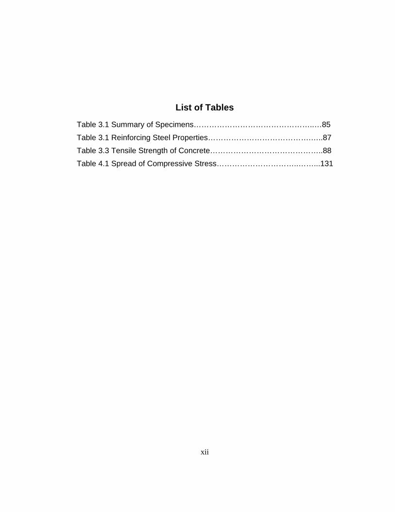
List of Tables
Table 3.1 Summary of Specimens………………………………………..…85
Table 3.1 Reinforcing Steel Properties………………………………….…..87
Table 3.3 Tensile Strength of Concrete……………………………………..88
Table 4.1 Spread of Compressive Stress…………………………..……...131
xii

List of Figures
Figure 1.1 Strut-and-Tie Models and As-Built Reinforcing for TxDOT
Misplaced Bent ........................................................................ 4
Figure 1.2 Bottle-Shaped Strut Capacity as a Function of the Angle
with an Adjacen TensionTie…………………………………….10
Figure 1.3 Bottle-Shaped Strut Capacity as a Function of the Confining
Reinforcement Ratio .............................................................. 11
Figure 2.1 Strut-and-Tie models used in Sanders Specimens from
[44] ........................................................................................ 20
Figure 2.2 Modified Strut-and-Tie Model to Include the Full Plastic
Capacity from [44]…………………………………………… ..... 20
Figure 2.3 Determining the Angle of Struts from [44] ............................... 21
Figure 2.4 Determination of the Tensile Ultimate Load from [44] ............. 22
Figure 2.5 Singular Node and Strut Dimensions from [44] ....................... 23
Figure 2.6 Pertinent Planes and Equations for Singular Node and
Strut Capacities from [44]…………………………………… ... 24
Figure 2.7 Example of Area Defined for Local Zone-General Zone from
[44] ........................................................................................ 25
Figure 2.8 Rules for STM from [51] .......................................................... 30
Figure 2.9 Comparison of Strut-and-Tie Models Varying Node
Geometry from [51] ................................................................ 31
Figure 2.10 Collapse of Shear Transfer from [51] .................................... 33
Figure 2.11 Two of Thompson’s CCT Node Specimens Measuring In-
Plane and Transverse Splitting of Bottle-shaped Struts
from [47] ................................................................................ 34
xiii
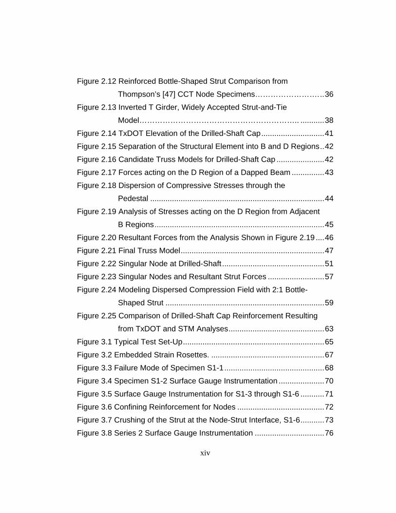
Figure 2.12 Reinforced Bottle-Shaped Strut Comparison from
Thompson’s [47] CCT Node Specimens……………………. .. 36
Figure 2.13 Inverted T Girder, Widely Accepted Strut-and-Tie
Model…………………………………………………….. ........... 38
Figure 2.14 TxDOT Elevation of the Drilled-Shaft Cap ............................. 41
Figure 2.15 Separation of the Structural Element into B and D Regions .. 42
Figure 2.16 Candidate Truss Models for Drilled-Shaft Cap ...................... 42
Figure 2.17 Forces acting on the D Region of a Dapped Beam ............... 43
Figure 2.18 Dispersion of Compressive Stresses through the
Pedestal ................................................................................ 44
Figure 2.19 Analysis of Stresses acting on the D Region from Adjacent
B Regions .............................................................................. 45
Figure 2.20 Resultant Forces from the Analysis Shown in Figure 2.19 .... 46
Figure 2.21 Final Truss Model .................................................................. 47
Figure 2.22 Singular Node at Drilled-Shaft ............................................... 51
Figure 2.23 Singular Nodes and Resultant Strut Forces .......................... 57
Figure 2.24 Modeling Dispersed Compression Field with 2:1 Bottle-
Shaped Strut ......................................................................... 59
Figure 2.25 Comparison of Drilled-Shaft Cap Reinforcement Resulting
from TxDOT and STM Analyses ............................................ 63
Figure 3.1 Typical Test Set-Up ................................................................. 65
Figure 3.2 Embedded Strain Rosettes. .................................................... 67
Figure 3.3 Failure Mode of Specimen S1-1 .............................................. 68
Figure 3.4 Specimen S1-2 Surface Gauge Instrumentation ..................... 70
Figure 3.5 Surface Gauge Instrumentation for S1-3 through S1-6 ........... 71
Figure 3.6 Confining Reinforcement for Nodes ........................................ 72
Figure 3.7 Crushing of the Strut at the Node-Strut Interface, S1-6 ........... 73
Figure 3.8 Series 2 Surface Gauge Instrumentation ................................ 76
xiv
Figure 3.9 Variables Involved in the Reinforcement of Series 2
Specimens………………………………………………… ......... 78
Figure 3.10 Effect of Reinforcing Schemes in Series 2 ............................ 79
Figure 3.11 Modified Bearing Plate Configuration .................................... 83
Figure 3.12 Typical Specimen Elevation for Use with Table 3.1 .............. 84
Figure 3.13 Details of Reinforcing Bar Placement .................................... 88
Figure 3.14 Specimen S3-4 Elevation at Testing ..................................... 89
Figure 3.15 Specimens S3-9 and S3-10 Non-Standard Details ............... 90
Figure 4.1 Specimens Used in Investigating Bottle-Shaped-Struts .......... 94
Figure 4.2 Tensile Failure Mechanism ..................................................... 97
Figure 4.3 Concrete Crushing at Node Failure Mechanism ...................... 98
Figure 4.4 Comparison of Failure Mechanisms for Confined and
Unconfined Specimens .......................................................... 99
Figure 4.5 Degradation of Shear-Transfer for Unconfined
Specimens ........................................................................... 100
Figure 4.6 Secondary Failure Mechanism Associated with “Heavily”
Reinforced Specimens………………………………………...102
Figure 4.7 Ultimate Capacities ............................................................... 104
Figure 4.8 Stress Redistribution ............................................................. 105
Figure 4.9 Dependence of Stress Redistribution on Reinforcement
Provided .............................................................................. 106
Figure 4.10 Effect of Reinforcement on Ultimate Capacity ..................... 107
Figure 4.11 Strain Recordings Indicating the Type of Failure
Mechanism…………………………………………….. ........... 110
Figure 4.12 Constitutive Relationship for Reinforcing Steel ................... 111
Figure 4.13 Average Reinforcement Stress in the Elastic Range for
Confined and Unconfined Specimens ................................. 112
xv

Figure 4.14 Reinforcing Bar Forces of Confined Specimens of
Different Geometric Loading Conditions .............................. 114
Figure 4.15 Reinforcing Bar Forces of Confined and Unconfined
Specimens ........................................................................... 115
Figure 4.16 Reinforcing Bar Forces for Three-Dimensional
Specimens ........................................................................... 116
Figure 4.17 Effect of Reinforcing Bars Parallel to the Load Axis of the
Specimen ............................................................................ 117
Figure 4.18 Effect of Variations of Reinforcement on the Ultimate
Capacity of the Specimen .................................................... 118
Figure 4.19 Verification of Constitutive Relationship for Compressive
Strains ................................................................................. 121
Figure 4.20 Tensile Strain Developed In Specimen S2-2 ....................... 122
Figure 4.22 Normalized Stress at Mid-height of the Specimen in the
ElasticRange……………………………………………… ....... 126
Figure 4.23 Normalized Stress at Mid-height of the Specimen in the
Elastic Range Cont…………………………………………….127
Figure 4.24 Normalized Stress at Mid-height of the Specimen after
Redistribution ...................................................................... 129
Figure 4.25 Normalized Stress at the Centerline of the Specimen after
Redistribution Cont. ............................................................. 130
Figure 5.1 Empirical Relationship Developed for the Test Specimens in
This Investigation................................................................. 136
Figure 5.2 Empirical Relationship from [34] and Comparison to Test
Data ..................................................................................... 137
Figure 5.3 Semi-Empirical Relationship from [39] and Comparison to
Test Data ............................................................................. 138
Figure 5.4 Typical Strut-and-Tie Models at Various Load Stages .......... 139
xvi
Figure 5.5 Stress Fields for a Typical Specimen Adapted from [33] ....... 140
Figure 5.6 Strut-and-Tie Models for Cracked and Uncracked Sections .. 142
Figure 5.7 Separation of Sub-Models in the Elastic Range .................... 143
Figure 5.8 Stress Distribution of Group I Specimens in the Elastic
Range .................................................................................. 144
Figure 5.9 Numerical Example of a Typical Strut-and-Tie Model ........... 146
Figure 5.10 Splitting Forces within a Pre-Tensioned Beam from [33] ..... 147
Figure 5.11 Comparison of Strut-and-Tie Models with [44] .................... 148
Figure 5.12 Force at the Vertical Face of the Node Split into Two
Components ........................................................................ 149
Figure 5.13 Production of the Strut-and-Tie Models for Each Specime .. 151
Figure 5.14 Comparison of Strut-and-Tie Models ................................... 154
Figure 5.15 State of Stress for Elements at the Nodal Region ............... 157
Figure 5.16 Stresses at Node Face and Node-Strut Interface from [47] . 158
Figure 5.17 Node Developed in Thompon’s [47] Headed Bar Tests ...... 159
Figure 5.18 AASHTO Provision for Reduced Concrete Capacity as a
Function of Lateral Strain from [41] ..................................... 160
Figure 5.19 Failure Stress as a Function of Transverse Strain .............. 162
Figure 5.20 Examples Of the Transition Stress Field ............................. 163
Figure 5.21 Transition Stress Field Adapted from [46] ........................... 165
Figure 5.22 ψ-νs Relationship with Differing Values of νns ...................... 166
Figure 5.23 Example Bi-axial Failure Criterion Developed from the ............
Experimental Program…………………………………………169
Figure 5.24 Effect of the Failure Criterion on the ψ-νs Relationship ........ 170
Figure 5.25 Explanation of the Point of Discontinuity in the ψ-νs
Relationship ......................................................................... 171
Figure 5.26 The Transition Stress Field Applied to the Singular Node of
the Specimens ..................................................................... 175
xvii

xviii
Figure 5.27 The Transition Stress Field Applied with Experimental Data176
Figure 5.28 Domain of the ψ - νs Relationship Used ............................... 177
Figure 5.29 Linear Regression of the Strut Capacity based on the Area
of Steel Provided Normalized to Area of the
Bearing Plate ....................................................................... 179
Figure 5.30 Transition Stress Field as a Function of the Reinforcement
Provided…………………………………………………… ....... 181
Figure 5.31 Stress Fields for Two Specimens ........................................ 183
Figure 5.32 Strut-and-Tie Model obtained from the Stress Fields in
Figure 5.31 .......................................................................... 184
Figure 5.33 Obtaining the Ultimate Load for a Strut from the Transition
Stress Field ......................................................................... 184
1
1.0 INTRODUCTION
1.1 HISTORICAL OVERVIEW
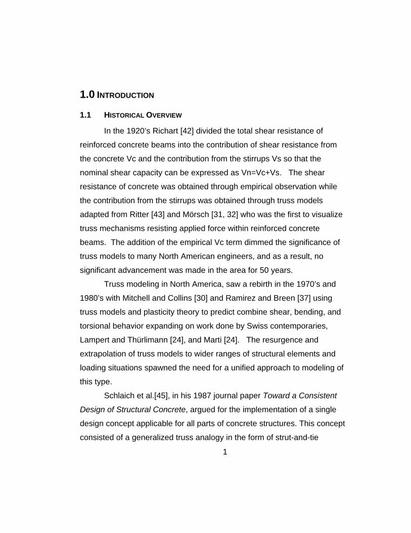
In the 1920’s Richart [42] divided the total shear resistance of
reinforced concrete beams into the contribution of shear resistance from
the concrete Vc and the contribution from the stirrups Vs so that the
nominal shear capacity can be expressed as Vn=Vc+Vs. The shear
resistance of concrete was obtained through empirical observation while
the contribution from the stirrups was obtained through truss models
adapted from Ritter [43] and Mörsch [31, 32] who was the first to visualize
truss mechanisms resisting applied force within reinforced concrete
beams. The addition of the empirical Vc term dimmed the significance of
truss models to many North American engineers, and as a result, no
significant advancement was made in the area for 50 years.
Truss modeling in North America, saw a rebirth in the 1970’s and
1980’s with Mitchell and Collins [30] and Ramirez and Breen [37] using
truss models and plasticity theory to predict combine shear, bending, and
torsional behavior expanding on work done by Swiss contemporaries,
Lampert and Thürlimann [24], and Marti [24]. The resurgence and
extrapolation of truss models to wider ranges of structural elements and
loading situations spawned the need for a unified approach to modeling of
this type.
Schlaich et al.[45], in his 1987 journal paper Toward a Consistent
Design of Structural Concrete, argued for the implementation of a single
design concept applicable for all parts of concrete structures. This concept
consisted of a generalized truss analogy in the form of strut-and-tie
2
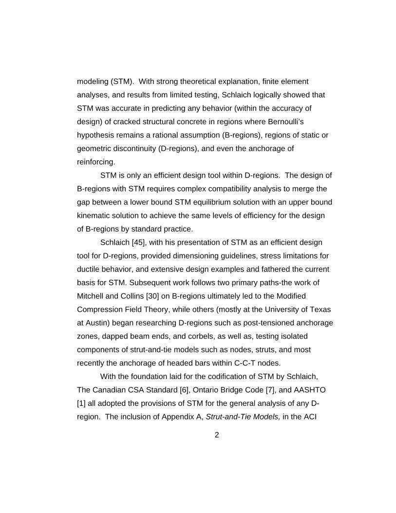
modeling (STM). With strong theoretical explanation, finite element
analyses, and results from limited testing, Schlaich logically showed that
STM was accurate in predicting any behavior (within the accuracy of
design) of cracked structural concrete in regions where Bernoulli’s
hypothesis remains a rational assumption (B-regions), regions of static or
geometric discontinuity (D-regions), and even the anchorage of
reinforcing.
STM is only an efficient design tool within D-regions. The design of
B-regions with STM requires complex compatibility analysis to merge the
gap between a lower bound STM equilibrium solution with an upper bound
kinematic solution to achieve the same levels of efficiency for the design
of B-regions by standard practice.
Schlaich [45], with his presentation of STM as an efficient design
tool for D-regions, provided dimensioning guidelines, stress limitations for
ductile behavior, and extensive design examples and fathered the current
basis for STM. Subsequent work follows two primary paths-the work of
Mitchell and Collins [30] on B-regions ultimately led to the Modified
Compression Field Theory, while others (mostly at the University of Texas
at Austin) began researching D-regions such as post-tensioned anchorage
zones, dapped beam ends, and corbels, as well as, testing isolated
components of strut-and-tie models such as nodes, struts, and most
recently the anchorage of headed bars within C-C-T nodes.
With the foundation laid for the codification of STM by Schlaich,
The Canadian CSA Standard [6], Ontario Bridge Code [7], and AASHTO
[1] all adopted the provisions of STM for the general analysis of any D-
region. The inclusion of Appendix A, Strut-and-Tie Models, in the ACI
318-02 raises the height of awareness of STM as a tool for analyzing and
detailing D-regions by practicing engineers. The increasing use of STM
by practicing engineers, variety of detailing problems, and range of
solutions possible using this design tool raise many questions that will
need to be answered through research and experimental study.
1.2 IMPETUS FOR STUDY
The decision by the Texas Department of Transportation (TxDOT)
to conduct Research Project 0-4371, Examination of the ASSHTO LRFD
Strut-and-Tie Specifications, was the result of questions and concerns
raised by bridge engineers regarding the application of the AASHTO strut-
and-tie model provisions to elements within their scope of design. The
limitations of the AASHTO STM provisions as well as the discomfort felt by
engineers initially using the these provisions when he displayed drawings
for various strut-and-tie models considered to verify the capacity of an as-
built bent cap section which had been misplaced in the field resulting in a
2 foot extension of the moment arm of the applied load. The strut-and-tie
models considered by TxDOT engineers and the as-built reinforcing of the
bent cap are shown in Figure 1.1.
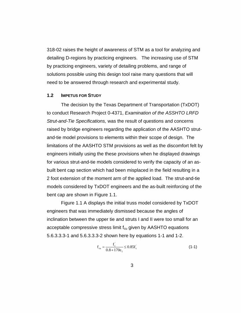
Figure 1.1 A displays the initial truss model considered by TxDOT
engineers that was immediately dismissed because the angles of
inclination between the upper tie and struts I and II were too small for an
acceptable compressive stress limit fcu given by AASHTO equations
5.6.3.3.3-1 and 5.6.3.3.3-2 shown here by equations 1-1 and 1-2.
'c
1
'c
cu f85.01708.0
ff ≤ε+
= (1-1)
3
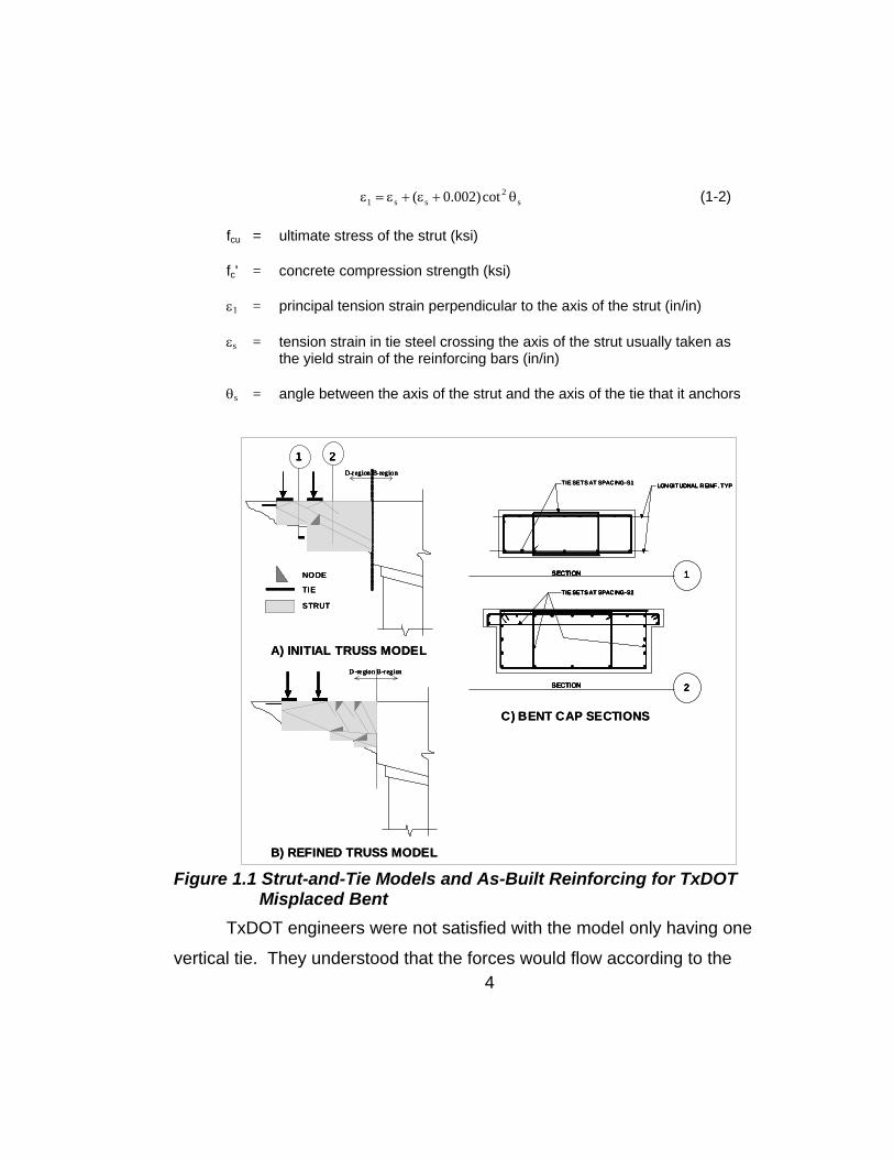
(1-2) s2
ss1 cot)002.0( θ+ε+ε=ε
fcu = ultimate stress of the strut (ksi)
fc' = concrete compression strength (ksi)
ε1 = principal tension strain perpendicular to the axis of the strut (in/in) εs = tension strain in tie steel crossing the axis of the strut usually taken as
the yield strain of the reinforcing bars (in/in)
θs = angle between the axis of the strut and the axis of the tie that it anchors
TIE SETS AT SPAC ING-S1 LON GITUDNAL R EINF. TYP
1SECTION
2SECTION
TIE SETS AT SPAC ING-S2
TIE SETS AT SPAC ING-S1 LON GITUDNAL R EINF. TYP
1SECTION
2SECTION
TIE SETS AT SPAC ING-S2
LON GITUDNAL R EINF. TYP
1SECTION
2SECTION
TIE SETS AT SPAC ING-S2
A) INITIAL TRUSS MODEL
B) REFINED TRUSS MODEL
C) BENT CAP SECTIONS
D-region B-region
1 2D-region B-region
1 2
D -re gion B-regionD -re gion B-region
NODE
TIE
STRUT
NODE
TIE
STRUT
TIE SETS AT SPAC ING-S1 LON GITUDNAL R EINF. TYP
1SECTION
2SECTION
TIE SETS AT SPAC ING-S2
TIE SETS AT SPAC ING-S1 LON GITUDNAL R EINF. TYP
1SECTION
2SECTION
TIE SETS AT SPAC ING-S2
LON GITUDNAL R EINF. TYP
1SECTION
2SECTION
TIE SETS AT SPAC ING-S2
A) INITIAL TRUSS MODEL
B) REFINED TRUSS MODEL
C) BENT CAP SECTIONS
D-region B-region
1 2D-region B-region
1 2
D -re gion B-regionD -re gion B-region
NODE
TIE
STRUT
NODE
TIE
STRUT
Figure 1.1 Strut-and-Tie Models and As-Built Reinforcing for TxDOT
Misplaced Bent TxDOT engineers were not satisfied with the model only having one
vertical tie. They understood that the forces would flow according to the
4

5
stiffness of the in-situ placement of the reinforcement, and a more
accurate model would therefore have a greater number of modeled
vertical ties. Figure 1.1 B shows the model after some refinement was
made and illustrates new uncertainties. The uncertainties about the model
include the assumed geometry of the nodes and stress field under the
applied loads, the geometry of the smeared nodes anchoring compressive
struts at vertical ties, the allocation of actual vertical stirrups to a single
modeled vertical tie, the geometry of struts anchoring vertical tension ties
(closed stirrups) if modeled according to AASHTO provisions 5.6.3.3.2,
and overall model optimization. The number of questions regarding the
refined model led the TxDOT engineers to abandon the STM solution
entirely.
It should be noted that bent cap STM is one prime for the
combination of finite element analyses (FEA) and STM, as recommended
by Schlaich [45]. The incorporation of a FEA would provide insight about
basic strut orientation and possible node geometries.; however, a FEA can
not answer all of the questions posed, especially those dealing with stress
limitations (which vary subjectively in different codes).
The example provided by TxDOT displayed the difficulty in
producing acceptable physical dimensions of a truss model that could be
used to check limiting compressive stresses in the concrete. Furthermore,
the stress limit for struts proposed by AASHTO given by equations 1-1
and 1-2 tend to cripple the overall model. The adoption of Appendix A,
Strut-and-Tie Models, into the ACI 318-02 building code, which is
congruent with the provisions for STM in the European FIB code [9],
6
provides another set of guidelines that can be evaluated using new
experimental data.
1.2.1 EVALUATION OF ACI 318-02 AND AASHTO LRFD STM PROVISIONS
In order to define inconsistencies with current ACI / AASHTO STM
provisions, and to highlight areas where research could be used to
improve STM guidelines, typical TxDOT designed structural elements
such as inverted T girders, pier caps, and pile caps, were alternately
designed using strut-and-tie models. The iterative truss models were
developed and dimensioned using the provisions provided by each code.
The acceptability of these models was based on current AASHTO and ACI
stress limitations coupled with serviceability requirements. The ratio of the
reinforcing steel cage weight resulting from each model to the reinforcing
steel cage weight produced by the original TxDOT design was computed
as a measure of model efficiency assuming that traditional TxDOT designs
provide safe, serviceable structures based on experience with and
performance of the traditional designs.
As a result of this exhaustive exercise, specific areas where
guidance is lacking in application of the provisions of each code, as well
as, specific discrepancies between the provisions in different codes
emerged and were noted. The following bulleted list summarizes these
difficulties and discrepancies:
7
discrepancies in the provisions for producing the physical geometry for singular
nodes
discrepancies in the provisions for producing the physical geometry of struts
anchored by closed ties
discrepancies in the provisions for the stress limits of struts
discrepancies in the provisions for the reinforcement of bottle shaped struts
1.2.2 BOTTLE-SHAPED STRUTS
The last two items in the preceding list are inter-related, and were
persistent problems in all the STM redesigns and represent prime topics
for experimental study. Schlaich [45] first suggested the need for
experimental study of the reinforcement of dispersed compression fields.
Sanders [44], Burdet [17] and Thompson [47] called for further
investigation into the capacity of struts in general after they observed that
of bottle-shaped struts constantly failed at higher levels of stress than
suggested by either AASHTO or CEB-FIP now FIB codes.
The AASHTO 5.6.3.3 STM provisions for strut capacity involve
checking the stress of the strut on the smallest area governed by adjacent
node geometry against a maximum stress produced by substituting
Equation 1-2 into 1-1. Equations 1-1 and 1-2 were developed by Collins
[30] based on data from deep beams and shell elements. The original
derivations were developed for ties composed of stirrups crossing the
paths of shear struts within deep beams at well-distributed intervals. The
adaptation of these equations to the general STM case has not been
verified by tests, nor has it been proven that these equations are adequate
for such situations as compact elements like corbels or three-dimensional
strut-and-tie models such as those which model pile caps [47].
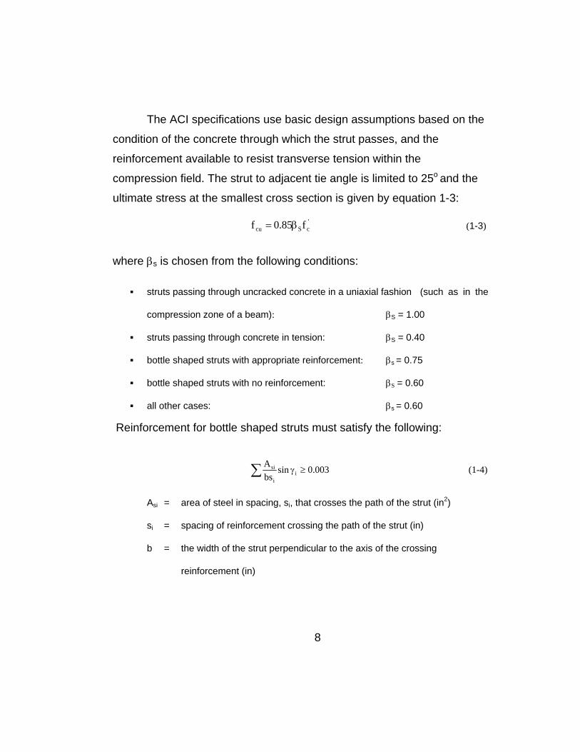
The ACI specifications use basic design assumptions based on the
condition of the concrete through which the strut passes, and the
reinforcement available to resist transverse tension within the
compression field. The strut to adjacent tie angle is limited to 25o and the
ultimate stress at the smallest cross section is given by equation 1-3:
(1-3) 'cScu f85.0f β=
where βs is chosen from the following conditions:
struts passing through uncracked concrete in a uniaxial fashion (such as in the
compression zone of a beam): βS = 1.00
struts passing through concrete in tension: βS = 0.40
bottle shaped struts with appropriate reinforcement: βs = 0.75
bottle shaped struts with no reinforcement: βS = 0.60
all other cases: βs = 0.60
Reinforcement for bottle shaped struts must satisfy the following:
∑ ≥γ 003.0sinbsA
ii
si (1-4)
Asi = area of steel in spacing, si, that crosses the path of the strut (in2)
si = spacing of reinforcement crossing the path of the strut (in)
b = the width of the strut perpendicular to the axis of the crossing
reinforcement (in)
8

9
γi = the angle between the axis of the strut and the axis of the crossing
reinforcement; γ must be greater than 40o if only one layer of
reinforcement crosses the strut
Furthermore, equation 1-4 may be replaced by proportioning
reinforcement based on 2:1 dispersion of compressive stresses. Three-
dimensional strut capacities are considered by ACI, not to be influenced
by reinforcing indicated in ACI RA.3.3:
Often, the confining reinforcement given in A.3.3 (1-3) is difficult to place
in three-dimensional structures such as pile caps. If the reinforcement is
not provided, the value of fcu given in A.3.3.3 (b) (βS = 0.60) is used.
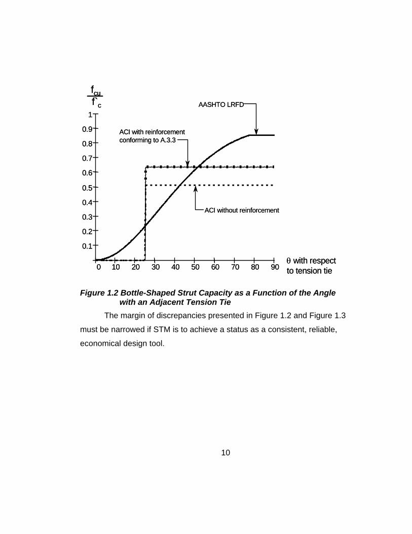
Figures 1.2 and 1.3 clearly depict the extreme differences between
the acceptance criteria as provided by ACI 318-02 Appendix A and
AASHTO LRFD strut-and-tie modeling provision for struts in which
compressive stresses have sufficient room to expand within the confines
of the structural element (bottle-shaped struts) creating associated
transverse tension-a frequently occurring condition in most reinforced
concrete structures. Figure 1.2 illustrates the capacities for bottle-shaped
struts anchoring tension ties. Figure 1.3 illustrates the capacity specified
for bottle-shaped struts not anchoring tension ties such as bottle shaped
struts adjoining two C-C-C Nodes. The differences illustrated by these
figures help to understand the a designer’s dilemma with a design based
on a strut-and-tie model acceptable for bridge structures (AASHTO) but
unacceptable for building structures (ACI).
0 10 20 30 40 50 60 70 80 90
0.1
0.2
0.3
0.4
0.5
0.6
0.7
0.8
0.9
1
θ with respect to tension tie
fcuf`c
ACI with reinforcementconforming to A.3.3
ACI without reinforcement
AASHTO LRFD
0 10 20 30 40 50 60 70 80 90
0.1
0.2
0.3
0.4
0.5
0.6
0.7
0.8
0.9
1
θ with respect to tension tie
fcuf`c
fcuf`c
ACI with reinforcementconforming to A.3.3
ACI without reinforcement
AASHTO LRFD
Figure 1.2 Bottle-Shaped Strut Capacity as a Function of the Angle with an Adjacent Tension Tie
The margin of discrepancies presented in Figure 1.2 and Figure 1.3
must be narrowed if STM is to achieve a status as a consistent, reliable,
economical design tool.
10

0 0.001 0.002 0.003 0.004 0.005 0.006
0.1
0.2
0.3
0.4
0.5
0.6
0.7
0.8
0.9
1
1
n
i
Asi
bsisin γi( )⋅∑
=
fcuf`c
AASHTO LRFD
ACI with reinforcementconforming to A.3.3
ACI without reinforcement
0 0.001 0.002 0.003 0.004 0.005 0.006
0.1
0.2
0.3
0.4
0.5
0.6
0.7
0.8
0.9
1
1
n
i
Asi
bsisin γi( )⋅∑
= 1
n
i
Asi
bsisin γi( )⋅∑
=
fcuf`c
fcuf`c
AASHTO LRFD
ACI with reinforcementconforming to A.3.3
ACI without reinforcement
Figure 1.3 Bottle-Shaped Strut Capacity as a Function of the Confining Reinforcement Ratio
1.3 RESEARCH OBJECTIVES AND SCOPE OF THESIS
The investigation into the application of ACI and AASHTO STM
provisions to TXDOT typical structural elements demonstrates the lack of
guidance within both provisions and the discrepancies between
provisions. Existing literature was reviewed to make sure that all
applicable data was included in resolving the problems noted. Those
areas where the experimental data was limited that questions and
11
12
discrepancies between the codes could not be addressed, were denoted
as areas for possible research.
The work presented herein constitutes Phase I of Research Project
0-4371, Examination of the ASSHTO LRFD Strut-and-Tie Specifications
sponsored by the Texas Department of Transportation. The objective of
Phase I was to study the compressive stress limitations for bottle-shaped
struts based on the effective amount of reinforcement available to confine
the strut and to unify the treatment of bottle-shaped struts by ACI and
AASHTO.

13
2.0 CURRENT STATE OF PRACTICE
2.1 INTRODUCTION
STM is a method that can both provide a conservative, lower bound
estimate of the ultimate capacity of a structural concrete section and
provide insight to proper detailing of structural concrete elements. The
method is most efficiently employed in regions where point loads,
reactions, and geometric discontinuities create states of stress that violate
simple beam theory. The method may be used for any region of structural
concrete elements regardless of the state of stress due to the method’s
strong basis in structural mechanics as argued by Schlaich et al [45].
Pragmatic North American designers, however, would find the method
tedious in application where simplified equations may be used that have
been substantiated by exhaustive experimental testing and result in ductile
structural behavior. In light of this attitude by the professional society,
STM has been delineated for use within disturbed regions (D-regions)
exclusively.
The STM method is a lower bound plasticity solution that will result
in a conservative estimate of the actual ultimate capacity of a section if: equilibrium is satisfied
at no point does the material exceed its failure criteria
detailing is such that sufficient ductility is provided to ensure plastic strains and
rotations
Since structural concrete is heterogeneous material consisting of a non-
ductile material (concrete) and ductile material (reinforcing steel) the last
two items of the bulleted list are dependent upon each other, and the
14
proper interaction of the two ensures plastic behavior by forcing ductile
failures of reinforcing steel prior to the non-ductile failures of concrete
crushing or anchorage failure.
STM is a relatively new concept to North American engineers;
although the basic concepts driving the method have been known and
employed by European engineers for over a hundred years, North
American research has not yet provided a consistent treatment of the
yielding criteria of concrete to ensure plastic behavior; instead, most
research has been concentrated on substantiating the method as a basic
design tool for specific structural elements. When applying the method in
practice, the production of the physical geometry of the truss models
employed in the STM method may be argued as the most frustrating
aspect of the overall STM process to engineers. STM allows complete
autonomy in the selection of a specific truss model. With more
experience engineers will find that while the absolute geometric definition
of struts, tie, and nodes and finding the exact location of these members
within the confines of the structural element under consideration are
important; they are not as critical as satisfying the three items in the
preceding bulleted list exclusively.
As an example, consider the bolt group connecting a gusset plate
to a structural steel section of a braced frame. The designer is only
concerned with equilibrium of forces in the analysis of the load path from
the brace to the column. The designer ensures that the yield criterion of
structural steel is met by specifying weld sizes, gusset plate thickness,
and the number of bolts and their spacing based on the simple equilibrium
15
calculation. The actual path the forces take from the brace through the
bolt group to the gusset plate through the welds and finally to the column
web or flange is inconsequential since equilibrium is satisfied. The
designer is able to achieve a safe design because the forces will
redistribute themselves as appropriate through a completely plastic media.
2.2 PROCEDURE FOR PRODUCING A STRUT-AND-TIE MODEL
After overall structural analysis has been performed to determine
exterior reactions, the designer must delineate the B and D-regions of the
structural element under consideration by using Saint Venant’s principle.
The adjacent B-region forces are determined through cracked section
analysis and placed on the adjacent D-region at the centroid on which
they act. The D-region can then be isolated and loaded with any exterior
reactions or loads and forces calculated from the B-region. The internal
flow of forces is then visualized through intuition, experience, or with the
help of a finite element analysis for complex situations. The designer then
chooses uni-axial struts and ties placed in the basic orientation of the
visualized forces. These struts and ties concentrate their curvature in
nodes to form a truss. The “stick-model” truss is then analyzed using
classical structural analysis to determine member forces. Reinforcement
is portioned for the corresponding tension force and the reinforcement is
placed such that the centroid of the reinforcement is concentric with the
centroid of the modeled tension tie. Singular node dimensions are then
estimated using code provisions. Singular nodes are defined as nodes
whose geometry can reasonably be ascertained due to the deviation of a

16
highly concentrated stress field such as applied load through rigid plates
with finite dimensions. On the other end of the spectrum, smeared nodes
are those in which stress fields are deviated over a smeared area. An
example of a smeared node is the deviation of a compressive stress field
crossed by evenly distributed reinforcement in which the actual deviation
of the stress field might spread over some length. An example of each
type of node is shown in Figure 2.1. Simultaneously with the estimation
of node dimensions, end critical strut dimensions are also defined. The
member forces calculated from the “stick-model” are then checked against
member capacities calculated by using the ultimate stress limits
(dependent on code) multiplying by the estimated area at critical locations.
Critical locations for singular nodes include the face under direct bearing
and the strut/node face. After assuring that stress levels are less than
ultimate, development lengths may be checked using code provisions.
This process is iterative and is repeated if stress levels at nodes and struts
exceed the maximum and/or anchorage is inadequate.
Detailed descriptions of the process are available in earlier
publications on STM, but none is as complete as Schlaich et al.’s [45]
1987 work, Toward a Consistent Design of Structural Concrete. However,
a comprehensive example regarding the physical production of a strut-
and-tie model including the findings of all current research from 1987 to
date is presented in 2.4.1.
17
2.3 EXPERIMENTAL INVESTIGATIONS
2.3.1 GENERAL
The scope of this research project encompassed the treatment of
stress limitations for bottle-shaped struts based on the amount of effective
reinforcement available within a concrete section to resist passive tensile
stresses transverse to the direction of applied load. Earlier publications do
not address this issue in depth; however, several publications described in
the proceeding sections form the foundation of experimental research that
produced guidelines for producing the physical geometry of strut-and-tie
models and provided guidelines for application of the method in order to
achieve safe and efficient designs.
2.3.2 NCHRP PROJECT 10-29
The National Cooperative Highway Research Program (NCHRP)
initiated Project 10-29 at UT in 1986 with the objective to develop design
procedures for end and intermediate anchorage zones for post-tensioned
girders, slabs, blisters, and diaphragms. In general, the investigation
proved STM to be a conservative approach for the design of anchorage
zones. The conclusions were supported by the results of more than 50
laboratory tests. As well as showing that STM is a valid overall design
approach, the project also provided the most comprehensive insight into
critical regions of strut-and-tie models, provided guidelines on model
dimensioning, and presented areas within STM that need further research.
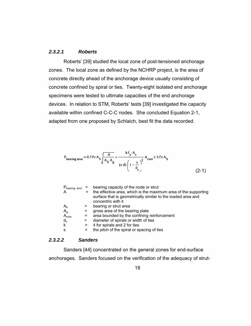
2.3.2.1 Roberts
Roberts’ [39] studied the local zone of post-tensioned anchorage
zones. The local zone as defined by the NCHRP project, is the area of
concrete directly ahead of the anchorage device usually consisting of
concrete confined by spiral or ties. Twenty-eight isolated end anchorage
specimens were tested to ultimate capacities of the end anchorage
devices. In relation to STM, Roberts’ tests [39] investigated the capacity
available within confined C-C-C nodes. She concluded Equation 2-1,
adapted from one proposed by Schlaich, best fit the data recorded.
_
Pbearing strut, 0.7 f'c⋅ AbA
Ab Ag⋅⋅
k fy⋅ As⋅
s d⋅( ) 1sdc
−⎛⎜⎝
⎞⎟⎠
2⋅
Acore⋅+ 3 f'c⋅ Ab⋅≤
_
Pbearing strut, 0.7 f'c⋅ AbA
Ab Ag⋅⋅
k fy⋅ As⋅
s d⋅( ) 1sdc
−⎛⎜⎝
⎞⎟⎠
2⋅
Acore⋅+ 3 f'c⋅ Ab⋅≤
(2-1)
Pbearing, strut = bearing capacity of the node or strut A = the effective area, which is the maximum area of the supporting surface that is geometrically similar to the loaded area and concentric with it Ab = bearing or strut area
Ag = gross area of the bearing plate Acore = area bounded by the confining reinforcement dc = diameter of spirals or width of ties k = 4 for spirals and 2 for ties s = the pitch of the spiral or spacing of ties
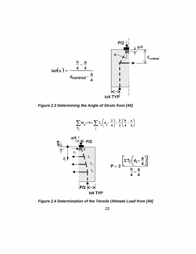
2.3.2.2 Sanders
Sanders [44] concentrated on the general zones for end-surface
anchorages. Sanders focused on the verification of the adequacy of strut-
18

19
and-tie models for predicting anchorage zone capacity. This was
achieved by developing specific strut-and-tie models for each specimen
which entailed the specific dimensioning of nodes and struts where
applicable, as well as, proportioning reinforcement to the modeled tie
force. The ultimate load of each model was taken as the minimum load
that caused either a compressive or tensile failure within the truss model.
Maximum compressive stresses were taken as a baseline of 0.7f`c plus
additional capacity if confinement was present as derived by Roberts [39].
Maximum strut member capacities were established by multiplying the
uniform stress limit to designated critical node and strut areas The
maximum compressive load was taken as the sum of the strut capacities
framing into the node ahead of the anchorage device. The maxim tensile
capacity of the specimen was established through the equilibrium of
specimens cracked down the specimen centerline with a known
distribution of reinforcement as shown in Figure 2.4. The minimum of the
maximum tensile capacity and the maximum compressive capacity was
taken as the specimen ultimate capacity and agreed well with
experimental results.
Sanders constructed 36 specimens in four categories as described
in the following: 17 concentric anchorage specimens with straight tendons
6 eccentric specimens with straight tendons
8 multiple anchorage specimens with straight tendons
4 inclined anchorage specimens with curved tendons.
The concentric anchorage specimens provided the most insight to STM as
it related to the scope of the research reported in this thesis. The models

used to predict the ultimate loads of these specimens are similar to those
used for bottle-shaped struts. Sanders used two basic strut-and-tie
models as shown in Figure 2.1.
singular node smeared nodesingular node smeared node
Figure 2.1 Strut-and-Tie models used in Sanders Specimens from
[44]
Figure 2.2 Modified Strut-and-Tie Model to Include the Full Plastic
Capacity from [44]
20
21
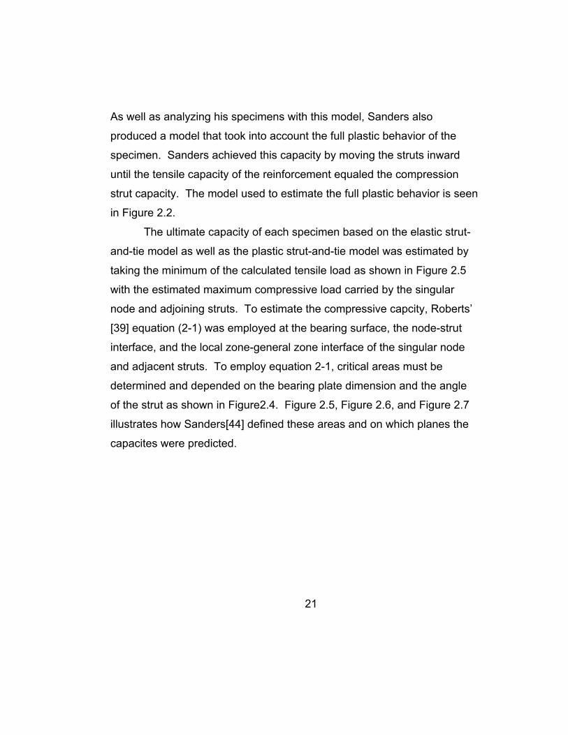
As well as analyzing his specimens with this model, Sanders also
produced a model that took into account the full plastic behavior of the
specimen. Sanders achieved this capacity by moving the struts inward
until the tensile capacity of the reinforcement equaled the compression
strut capacity. The model used to estimate the full plastic behavior is seen
in Figure 2.2.
The ultimate capacity of each specimen based on the elastic strut-
and-tie model as well as the plastic strut-and-tie model was estimated by
taking the minimum of the calculated tensile load as shown in Figure 2.5
with the estimated maximum compressive load carried by the singular
node and adjoining struts. To estimate the compressive capcity, Roberts’
[39] equation (2-1) was employed at the bearing surface, the node-strut
interface, and the local zone-general zone interface of the singular node
and adjacent struts. To employ equation 2-1, critical areas must be
determined and depended on the bearing plate dimension and the angle
of the strut as shown in Figure2.4. Figure 2.5, Figure 2.6, and Figure 2.7
illustrates how Sanders[44] defined these areas and on which planes the
capacites were predicted.
T1
T2
T3
h/4 TYP
P/2P/2a/4
dcentroidα
tan α( )h4
a4
−
dcentroida4
−
T1
T2
T3
h/4 TYP
P/2P/2a/4
dcentroidα
T1
T2
T3
h/4 TYP
P/2P/2a/4
dcentroidα
tan α( )h4
a4
−
dcentroida4
−
Figure 2.3 Determining the Angle of Struts from [44]
_
T j
Mx∑ 0
j
Tj d j14
−⎛⎜⎝
⎞⎟⎠
⋅∑ P2
h4
a4
−⎛⎜⎝
⎞⎟⎠
⋅−
P 2Σ Tj dj
a4
−⎛⎜⎝
⎞⎟⎠
⋅⎡⎢⎣
⎤⎥⎦
h4
a4
−
T1
T2
T3
h/4 TYP
P/2P/2
P/2
x
a/4
dj
C3
a/4
P 2Σ Tj dj
a4
−⎛⎜⎝
⎞⎟⎠
⋅⎡⎢⎣
⎤⎥⎦
h4
a4
−
T1
T2
T3
h/4 TYP
P/2P/2
P/2
x
a/4
dj
C3
a/4
_
T j
Mx∑ 0
j
Tj d j14
−⎛⎜⎝
⎞⎟⎠
⋅∑ P2
h4
a4
−⎛⎜⎝
⎞⎟⎠
⋅−
P 2Σ Tj dj
a4
−⎛⎜⎝
⎞⎟⎠
⋅⎡⎢⎣
⎤⎥⎦
h4
a4
−
T1
T2
T3
h/4 TYP
P/2P/2
P/2
x
a/4
dj
C3
a/4
P 2Σ Tj dj
a4
−⎛⎜⎝
⎞⎟⎠
⋅⎡⎢⎣
⎤⎥⎦
h4
a4
−
T1
T2
T3
h/4 TYP
P/2P/2
P/2
x
a/4
dj
C3
a/4
_
T j
Mx∑ 0
j
Tj d j14
−⎛⎜⎝
⎞⎟⎠
⋅∑ P2
h4
a4
−⎛⎜⎝
⎞⎟⎠
⋅−
P 2Σ Tj dj
a4
−⎛⎜⎝
⎞⎟⎠
⋅⎡⎢⎣
⎤⎥⎦
h4
a4
−
T1
T2
T3
h/4 TYP
P/2P/2
P/2
x
a/4
dj
C3
a/4
T1
T2
T3
h/4 TYP
P/2P/2
P/2
x
a/4
dj
C3
a/4
P 2Σ Tj dj
a4
−⎛⎜⎝
⎞⎟⎠
⋅⎡⎢⎣
⎤⎥⎦
h4
a4
−
T1
T2
T3
h/4 TYP
P/2P/2
P/2
x
a/4
dj
C3
a/4
T1
T2
T3
h/4 TYP
P/2P/2
P/2
x
a/4
dj
C3
a/4
Figure 2.4 Determination of the Tensile Ultimate Load from [44]
22

Figure 2.5 Singular Node and Strut Dimensions from [44]
23
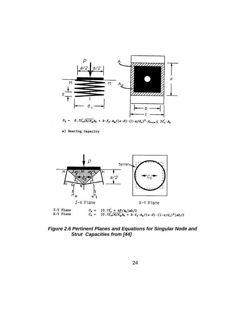
Figure 2.6 Pertinent Planes and Equations for Singular Node and Strut Capacities from [44]
24
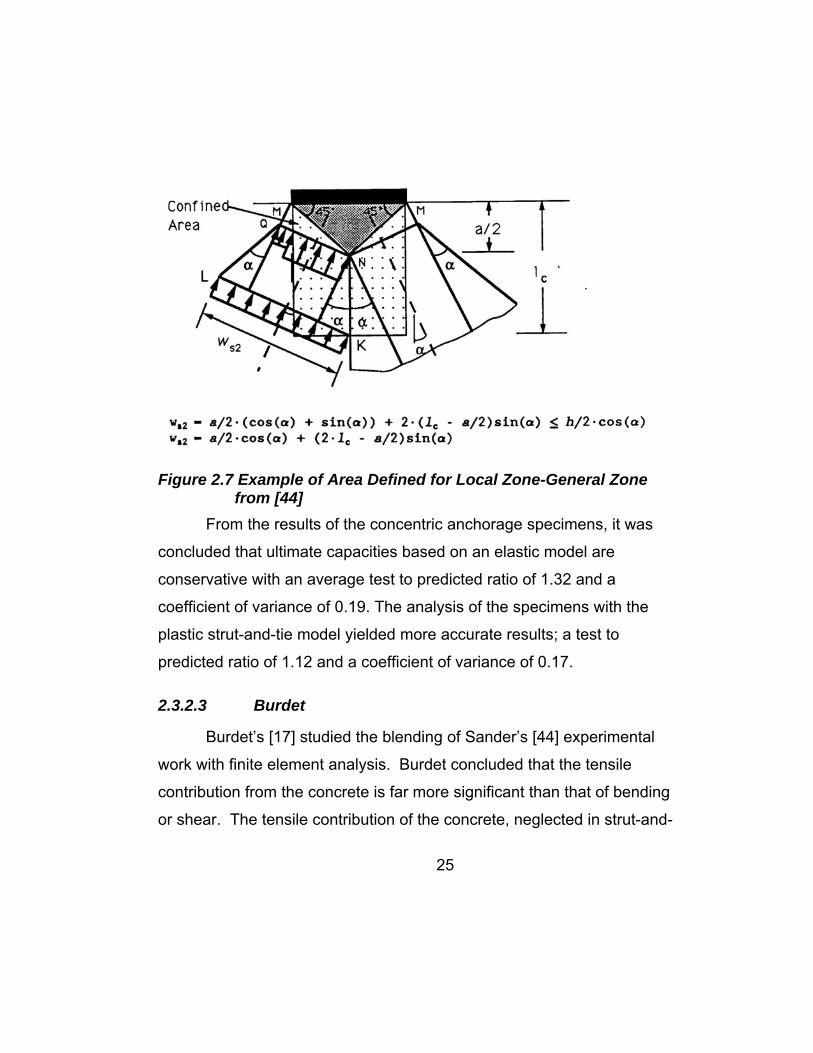
Figure 2.7 Example of Area Defined for Local Zone-General Zone from [44]
From the results of the concentric anchorage specimens, it was
concluded that ultimate capacities based on an elastic model are
conservative with an average test to predicted ratio of 1.32 and a
coefficient of variance of 0.19. The analysis of the specimens with the
plastic strut-and-tie model yielded more accurate results; a test to
predicted ratio of 1.12 and a coefficient of variance of 0.17.
2.3.2.3 Burdet
Burdet’s [17] studied the blending of Sander’s [44] experimental
work with finite element analysis. Burdet concluded that the tensile
contribution from the concrete is far more significant than that of bending
or shear. The tensile contribution of the concrete, neglected in strut-and-
25

26
tie models, manifested itself by forcing concrete crushing leading to brittle
failure and overall low ductility of the specimens. Significant redistribution
of stresses was apparent which was substantiated by the behavior of
specimens with tensile reinforcement placed in areas away from the
elastic centroid of tensile stress whose performance was not substantially
different from the behavior of those specimens with tensile reinforcement
placed at the elastic centroid of tensile stresses. Furthermore, Burdet
stated that the most important aspect for achieving good behavior in
service and ultimate states is proportioning reinforcement based on
equation 2-2, and placing this reinforcement at the elastic centroid of
tensile stress given by equation 2-3. Burdet also concluded that concrete
can resist compressive stresses in the about 0.75f`c if it is not confined by
reinforcement or surrounding concrete, such conditions exist at the local-
general zone interface and, in some cases, at the node-strut interface. He
recommended that a check of concrete compressive stresses at a
distance equal to lateral dimension of the anchorage device be made
using equation 2-4. Finally, Burdet concluded that the accuracy of the
strut-and-tie model for predicting compressive capacity decreases with the
complexity of the model and, for these cases numerical analyses are
desirable.

Tburst 0.25 P 1ah
−⎛⎜⎝
⎞⎟⎠
⋅ 0.5 P⋅ sin α( )⋅+
dcentroid 0.5 12eh
−⎛⎜⎝
⎞⎟⎠
⋅ 0.5 e⋅ sin α( )⋅+
fca
0.60 Pu⋅
a b⋅1
1 a1
b1t
−
⎛⎜⎜⎝
⎞⎟⎟⎠
+
⋅ 0.75f'c≤
(2-2)
(2-3)
(2-4)
Tburst = tensile bursting reinforcement dcentroid = centroid of tensile stresses Fca = compressive at distance a ahead of anchorage device P = Total load applied
a = lateral dimension of anchorage device h = transverse dimension of the cross section in direction considered α = angle of inclination of the tendon with respect to the centerline of
the member b = side length of anchorage device in the thin direction of the
specimen t = thickness of the cross section
2.3.2.4 Wollman
As the final phase of Project 10-29, Wollman [51] investigated the
influence of end reactions on anchorage zones, as well as, investigated
the applicability of strut-and-tie models to ribs, blisters, and diaphragms.
Wollman’s conclusions were based on all previous work done by Roberts
[39], Sanders [44], and Burdet [17]. To facilitate the implementation of
27

28
STM, Wollman [51] proposed rules for developing strut-and-tie models
shown in Figure 2.8
Wollman further substantiated the work done by Sanders [44] in
producing the physical geometry of the strut-and-tie models used to
analyze anchorage zones. The physical geometry of the models created
by Sanders, Burdet and finally Wollman reflect bottle-shaped struts with a
confined singular node at the anchorage device and were the foundation
for the physical geometry of the strut-and-tie models used to describe the
behavior of specimens for this research project.
To substantiate the work done by Sanders [44] in regard to the
physical geometry of nodes and struts, he made a simple comparison of
models used in the analysis of specimens that had slight but significant
differences. The main differences were concentrated in the geometry of
the singular nodes, but manifested themselves in the bearing capacity of
the struts. The impetus of the second analysis by Wollman was that a
node with a smaller dimension in the plane of loading (a/4 dimension in
Figure 2.4) would ultimately reduce the amount of bursting reinforcement
necessary by increasing the moment arm of the tensile reinforcement.
Sanders [44] used non-hydrostatic node geometries in his analysis with
the height of the node always equal to half the dimension of the
anchorage device. Wollman [51] compared Sanders [44] models to ones
that included non-hydrostatic nodes and fan shaped struts that have non-
uniform stress distributions. The details and structural mechanics behind
Wollman’s [51] analysis are complicated and not necessarily relevant to
the scope of this thesis, and therefore, are not shown here. The

29
importance of Wollman’s [51] second analysis can be seen in Figure 2.10
which shows that the ultimate loads predicted by each assumed geometry
of the singular node are very similar, and that assuming the struts to have
uniform stress distribution not exceeding 0.7f`c is a reasonable
assumption compared to the alternative.
Other important conclusions from this comparison include, the fact

Figure 2.8 Rules for STM from [51]
30

Method A Sanders non-hydrostatic node geometry
Method B hydrostatic node and and fan-shaped struts
f/fcmax level of stress in the struts relative to 0.7f’c
ao height of node in the direction of loading assumedto be a/4 for method A
Method A Sanders non-hydrostatic node geometry
Method B hydrostatic node and and fan-shaped struts
f/fcmax level of stress in the struts relative to 0.7f’c
ao height of node in the direction of loading assumedto be a/4 for method A
Figure 2.9 Comparison of Strut-and-Tie Models Varying Node
Geometry from [51]
31
32
that only live end model for beam 3 predicted a failure of concrete
crushing and all others predicted a failure of the tensile reinforcement, yet
the laboratory experiments all failed by concrete crushing at the local
zone-general zone interface. In another important comparison conducted
by Wollman [51], he predicted the failure of the same specimens using
only a simple compressive stress check provided by Burdet [17] using
equation 2-4. The four laboratory specimens yielded results with mean
test to predicted ration of 1.09 with a standard deviation of 0.13 using
equation 2-4.
Further adding insight relative to the scope of this investigation,
Wollman [51] made a concise statement about the role of bursting
reinforcement within the end-anchorage specimens. He concluded that
role of bursting reinforcement was to resist direct tensile stress, not to
increase effective concrete strength in compression. The bursting
reinforcement plays no role until the concrete has cracked at which point
the reinforcement is utilized through the redistribution of stresses resulting
from the loss of stiffness available from the concrete acting in tension.
After cracking has occurred, the main role of the reinforcement is to
reduce the dispersion of compression radiating from the point of load
application. If no reinforcement is present then the failure mode is purely
related to the loss of shear friction at the strut-node interface as illustrated
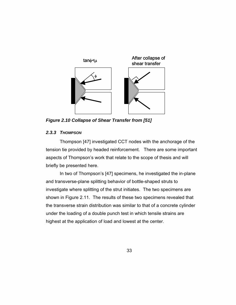
in Figure 2.10.
φ
tanφ<μ After collapse of shear transfer
φ
tanφ<μ After collapse of shear transfer
Figure 2.10 Collapse of Shear Transfer from [51]
2.3.3 THOMPSON
Thompson [47] investigated CCT nodes with the anchorage of the
tension tie provided by headed reinforcement. There are some important
aspects of Thompson’s work that relate to the scope of thesis and will
briefly be presented here.
In two of Thompson’s [47] specimens, he investigated the in-plane
and transverse-plane splitting behavior of bottle-shaped struts to
investigate where splitting of the strut initiates. The two specimens are
shown in Figure 2.11. The results of these two specimens revealed that
the transverse strain distribution was similar to that of a concrete cylinder
under the loading of a double punch test in which tensile strains are
highest at the application of load and lowest at the center.
33

11 S
train
Gag
es10
@ 2
”
11 S
train
Gag
es10
@ 2
”
1.5” plinth
10 Strain Gages
9 @ 2”
1.5” plinth
10 Strain Gages
9 @ 2”
A) Strain Gauges measuring Transverse Splitting Strains
B) Strain Gauges measuring In-Plane Splitting Strains
11 S
train
Gag
es10
@ 2
”
11 S
train
Gag
es10
@ 2
”
1.5” plinth
10 Strain Gages
9 @ 2”
1.5” plinth
10 Strain Gages
9 @ 2”
A) Strain Gauges measuring Transverse Splitting Strains
B) Strain Gauges measuring In-Plane Splitting Strains Figure 2.11 Two of Thompson’s CCT Node Specimens Measuring In-
Plane and Transverse Splitting of Bottle-shaped Struts from [47]
34

35
This is opposite to the behavior typically modeled using bottle-shaped
struts. The in-plane strain results indicated that splitting occurred at the
CCT node, and strains increased at the center once a crack parallel to the
strut formed. The capacity of the section reached ultimate just before this
crack formed and lost capacity slowly as further load was applied and the
crack widened. This might indicate that, if the strut was reinforced across
the crack, the final capacity could have been higher.
Thompson also investigated the efficiency factor for the bottle-
shaped struts produced through the geometry and loading of his
specimens. The efficiency factor is defined as the ultimate stress on the
strut face normalized to f`c. The area of the strut face was determined by
the bearing plate and the head size of the headed bar and assumed to be
trapezoidal. The efficiency factors calculated by Thompson [47] were far
greater than those provided by ACI 318-02. The results also refute the
AASHTO LRFD provisions that if accurate, would have shown at least a
trend of higher efficiency as the strut angle increased using a simple yield
strain of .002 in equations 1-1 and 1-2.
Finally, Thompson’s series of confined specimen tests which are
the most likely configuration of reinforced bottle-shaped struts within
structural concrete having reinforcement provided as closed stirrups
showed no trend in of increased strut capacity as the confinement ratio of
As/(bs) increased. Comparing the five confined specimens with
specimens that had the same overall configuration with out the stirrup
reinforcement (control specimens) showed that the strut capacity was
more sensitive to the tension reinforcement end detail; hence the strut

capacity was more sensitive to the node formed by the anchorage of
reinforcement. A plot comparing the like specimens with and with out
confinement is shown in Figure 2.12 which displays the maximum strut
force normalized with respect to the concrete strength.
0
0.2
0.4
0.6
0.8
1
1.2
STRAIGHT HEADED HOOK
WHead
HHead
WPlate
AStrutWHead
HHead
WPlate
AStrut
Fstrut
Asbs = 0.006
= 0.012Asbs
no confinement
Asbs = 0.006
= 0.012Asbs
no confinement
Asbs = 0.006AsbsAsbs = 0.006
= 0.012Asbs = 0.012AsbsAsbs
no confinement
Fstrut f`c
0
0.2
0.4
0.6
0.8
1
1.2
STRAIGHT HEADED HOOK
WHead
HHead
WPlate
AStrutWHead
HHead
WPlate
AStrut
Fstrut
WHead
HHead
WPlate
AStrutWHead
HHead
WPlate
AStrut
Fstrut
Asbs = 0.006
= 0.012Asbs
no confinement
Asbs = 0.006
= 0.012Asbs
no confinement
Asbs = 0.006AsbsAsbs = 0.006
= 0.012Asbs = 0.012AsbsAsbs
no confinement
Fstrut f`c
Fstrut f`c
Figure 2.12 Reinforced Bottle-Shaped Strut Comparison from Thompson’s [47] CCT Node Specimens
36

37
The bearing face of the strut is not represented in the plot because
it remains constant with respect to the main tension reinforcement end
detail.
2.4 DESIGN EXAMPLE
To best illustrate the current state of practice a design example is
shown is the following section with additional step-by-step commentary.
The design example is intended to display all of current modeling
techniques acquired throughout the literature with emphasis on the
findings presented in section 2.4. The design example is only bounded by
the limitations set forth by the current ACI 318-02 Appendix A and the
AASHTO LRFD 5.6.3 STM provisions in regard to stress limitations and
guidelines set forth for the physical geometry of struts, ties, and nodes.
Calculations are presented in parallel to display similarities and
differences of the provisions of each major North American code authority.
The drilled shaft cap is presented here whose physical geometry
creates an ideal situation for the designer to exercise his own judgment in
the creation of the truss model, autonomous from any other condition
other than satisfying internal and external equilibrium.
This element was chosen for illustration before other commonly
illustrated models such as the strut-and-tie model for an inverted T-girder
shown in Figure 2.13. Models such as the one shown in Figure 2.13 have
been reproduced in many publications and are “boiler plate” reproductions
that do not display the wide variability with the STM process. The goal of
the design example presented in 2.4.1 is to display the range of modeling
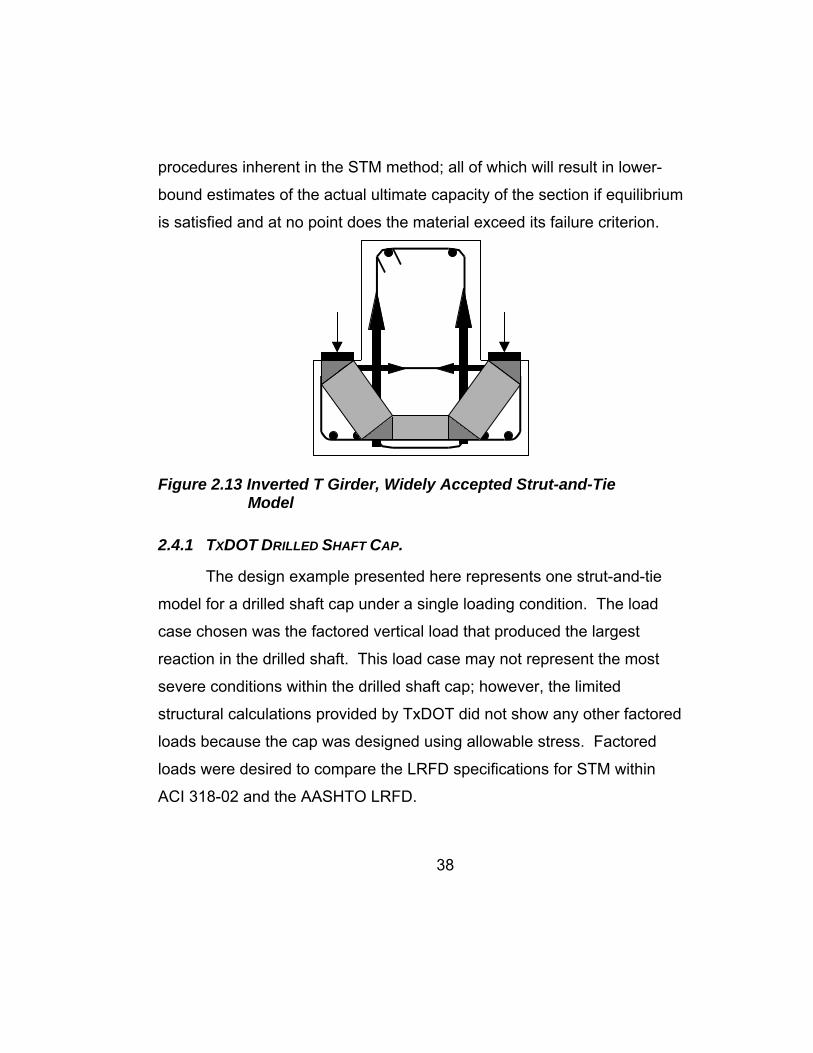
procedures inherent in the STM method; all of which will result in lower-
bound estimates of the actual ultimate capacity of the section if equilibrium
is satisfied and at no point does the material exceed its failure criterion.
Figure 2.13 Inverted T Girder, Widely Accepted Strut-and-Tie Model
2.4.1 TXDOT DRILLED SHAFT CAP.
The design example presented here represents one strut-and-tie
model for a drilled shaft cap under a single loading condition. The load
case chosen was the factored vertical load that produced the largest
reaction in the drilled shaft. This load case may not represent the most
severe conditions within the drilled shaft cap; however, the limited
structural calculations provided by TxDOT did not show any other factored
loads because the cap was designed using allowable stress. Factored
loads were desired to compare the LRFD specifications for STM within
ACI 318-02 and the AASHTO LRFD.
38

39
The drilled shaft cap provides the base for a 45 ft. tall precast
segmental column supporting an elevated highway. The TxDOT drawing
showing an details of this structural element is shown in Figure 2.15.
To begin the process of designing an element using the strut-and-
tie method, the designer must first establish the B and D regions of the
structural element under consideration as shown in Figure 2.16. Once the
D-region is established, a truss model may be chosen such that the
tension and compression members are aligned with direction of principal
tensile and compressive stresses. A finite element analysis may be
performed at this point to determine the elastic flow of stresses from which
the orientation of members within the truss model can be more easily
visualized. For this example, a finite element analysis proves to be
superfluous because the flow of forces from the column to the drilled
shafts through the cap can easily be visualized.
Once the flow of forces can be visualized through, experience,
intuition, or the help of a finite element analysis, a truss model can be
established with members orientated in the general direction of these
forces. Some candidate truss models are shown in Figure 2.17
Since strut-and-tie modeling is a lower bound solution, any model
chosen which is in equilibrium with applied load, has sufficient ductility to
ensure plastic rotations, and meets all specified failure criteria is
acceptable and will provide a conservative or lower bound estimate of the
actual ultimate load.
This selection of the strut-and-tie model often proves to be most
difficult for designers who would like to immediately find the optimum
40
solution for each problem. To help designers meet this objective some
rules of thumb regarding the optimization of a model for the most
favorable structural behavior have been defined by Schlaich [45],
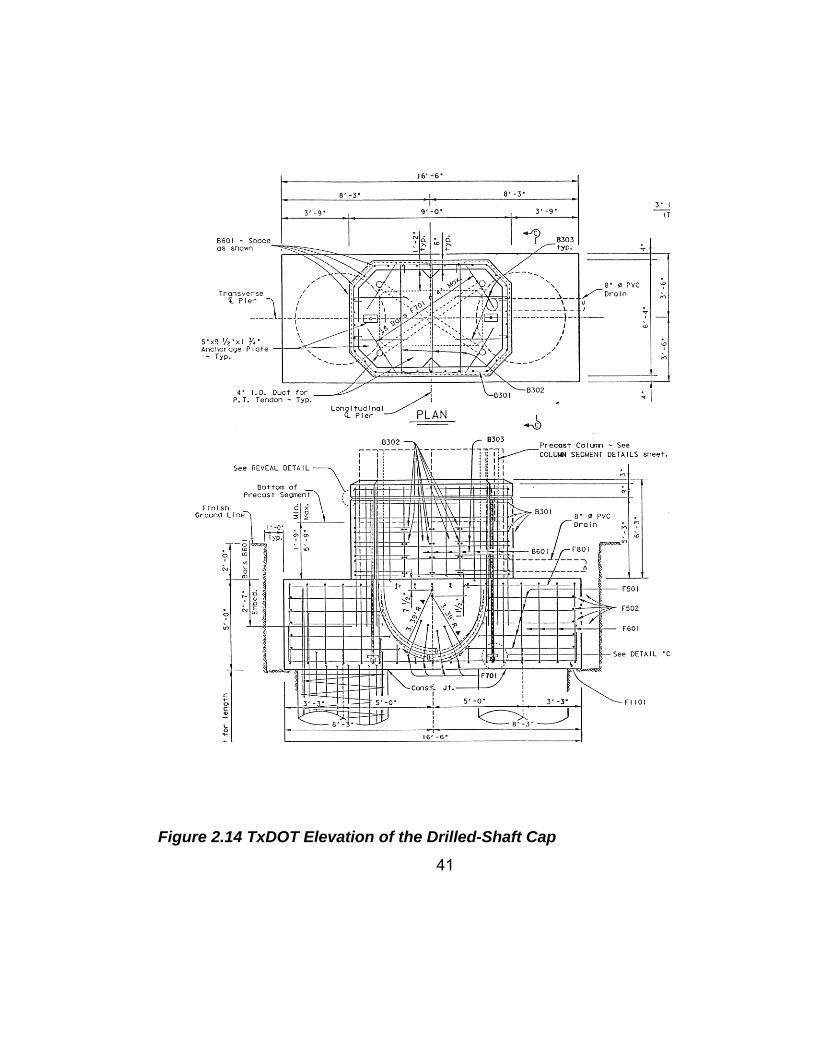
Figure 2.14 TxDOT Elevation of the Drilled-Shaft Cap
41
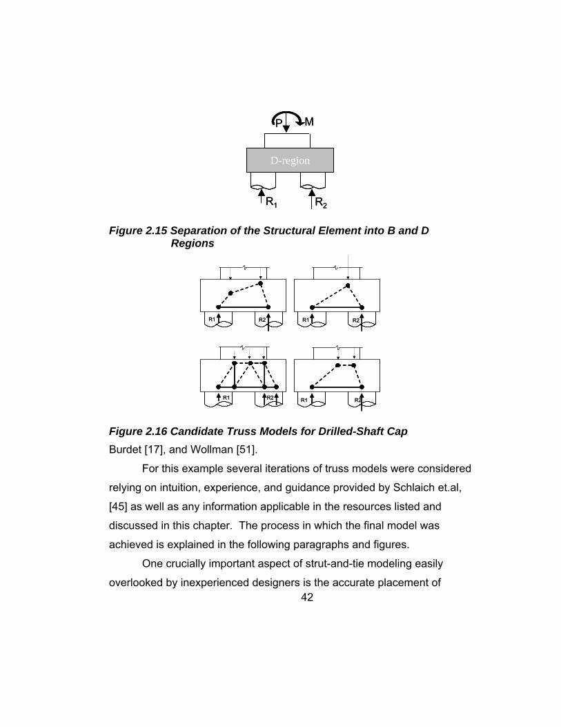
D-region
MP
R2R1
D-region
MP
R2R1
Figure 2.15 Separation of the Structural Element into B and D Regions
R1 R2
R1 R2
R1 R2
R1 R2
R1 R2
R1 R2
R1 R2
R1 R2
Figure 2.16 Candidate Truss Models for Drilled-Shaft Cap Burdet [17], and Wollman [51].
For this example several iterations of truss models were considered
relying on intuition, experience, and guidance provided by Schlaich et.al,
[45] as well as any information applicable in the resources listed and
discussed in this chapter. The process in which the final model was
achieved is explained in the following paragraphs and figures.
42
One crucially important aspect of strut-and-tie modeling easily
overlooked by inexperienced designers is the accurate placement of
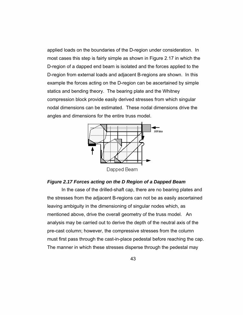
applied loads on the boundaries of the D-region under consideration. In
most cases this step is fairly simple as shown in Figure 2.17 in which the
D-region of a dapped end beam is isolated and the forces applied to the
D-region from external loads and adjacent B-regions are shown. In this
example the forces acting on the D-region can be ascertained by simple
statics and bending theory. The bearing plate and the Whitney
compression block provide easily derived stresses from which singular
nodal dimensions can be estimated. These nodal dimensions drive the
angles and dimensions for the entire truss model.
Figure 2.17 Forces acting on the D Region of a Dapped Beam In the case of the drilled-shaft cap, there are no bearing plates and
the stresses from the adjacent B-regions can not be as easily ascertained
leaving ambiguity in the dimensioning of singular nodes which, as
mentioned above, drive the overall geometry of the truss model. An
analysis may be carried out to derive the depth of the neutral axis of the
pre-cast column; however, the compressive stresses from the column
must first pass through the cast-in-place pedestal before reaching the cap.
The manner in which these stresses disperse through the pedestal may
43
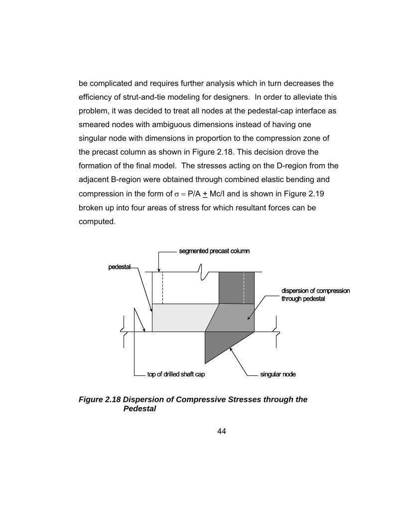
be complicated and requires further analysis which in turn decreases the
efficiency of strut-and-tie modeling for designers. In order to alleviate this
problem, it was decided to treat all nodes at the pedestal-cap interface as
smeared nodes with ambiguous dimensions instead of having one
singular node with dimensions in proportion to the compression zone of
the precast column as shown in Figure 2.18. This decision drove the
formation of the final model. The stresses acting on the D-region from the
adjacent B-region were obtained through combined elastic bending and
compression in the form of σ = P/A + Mc/I and is shown in Figure 2.19
broken up into four areas of stress for which resultant forces can be
computed.
dispersion of compressionthrough pedestal
segmented precast column
top of drilled shaft cap
pedestal
singular node
dispersion of compressionthrough pedestal
segmented precast column
top of drilled shaft cap
pedestal
singular node
Figure 2.18 Dispersion of Compressive Stresses through the Pedestal
44

A1 A2 A3 A4
Plan view of stressesacting on the pedestal from the precast column above,simplified for analysis
ii
PA
McI
iii iv v vi viii
P 4444 k⋅
M 8733 k⋅ ft⋅
σi 0.006− ksi⋅
σii 0.274 ksi⋅
σiii 0.628 ksi⋅
σiv 0.834 ksi⋅
σv 1.04 ksi⋅
σvi 1.39 ksi⋅
σvii 1.67 ksi⋅
A1 A2 A3 A4
Plan view of stressesacting on the pedestal from the precast column above,simplified for analysis
ii
PA
McI
iii iv v vi viii
P 4444 k⋅
M 8733 k⋅ ft⋅
σi 0.006− ksi⋅
σii 0.274 ksi⋅
σiii 0.628 ksi⋅
σiv 0.834 ksi⋅
σv 1.04 ksi⋅
σvi 1.39 ksi⋅
σvii 1.67 ksi⋅
Figure 2.19 Analysis of Stresses acting on the D Region from
Adjacent B Regions The sub-division of the stresses into resultant forces is another
matter that must be taken into consideration. A large number of sub-
divisions will yield a more accurate depiction of the flow of forces;
however, the designer must balance the number of sub-divisions with
simplicity of analysis in order to achieve the efficiency of this design tool.
After some iteration a decision to divide the pedestal into 4 distinct areas
was arrived that balanced an accurate depiction of the flow of forces and
simplicity of analysis. The four resultant forces locate the nodes of the
upper chord of the truss model. The resultant forces acting on A1 through
A4 in Figure 2.19 is shown in Figure 2.20.
45

17.4”
9”14.5”
97.1”
68.0”
41.1”
17.0” 164K
455K
355K
1244K
isometric view of ½ of the drilled-shaft cap topsurface and resultantforce locations
resu
ltant
forc
e fro
m A
4
resu
ltant
forc
e fro
m A
3re
sulta
nt fo
rce
from
A1
resu
ltant
forc
e fro
m A
2
17.4”
9”14.5”
97.1”
68.0”
41.1”
17.0” 164K
455K
355K
1244K
isometric view of ½ of the drilled-shaft cap topsurface and resultantforce locations
resu
ltant
forc
e fro
m A
4
resu
ltant
forc
e fro
m A
3re
sulta
nt fo
rce
from
A1
resu
ltant
forc
e fro
m A
2
Figure 2.20 Resultant Forces from the Analysis Shown in Figure 2.19 Figure 2.20 clearly shows the three-dimensional nature of this
problem; however, for ease of analysis the forces on both sides of the axis
of symmetry were added and placed at the centerline of the cap. Once
the location of the resultant forces are known the node locations of the
upper chord of the truss model at the pedestal-cap interface are defined
and the truss model can be finalized. The final truss model chosen was
shown in Figure 2.21.
46

Singular Sub-node
Smeared Node
Tension Tie
Compression Strut
X
X Singular Sub-node
Smeared Node
Tension Tie
Compression Strut
X
X
P 4444 k⋅:= M 8733 k⋅ ft⋅:=
P1 328 k⋅:=
P2 710 k⋅:=
P3 910 k⋅:=
P4 2488 k⋅:=
R1 1406 k⋅:=
R11 328 k⋅:=
R12 1078 k⋅:=
R2 3038 k⋅:=
R21 550 k⋅:=
R22 1628 k⋅:=
R23 860 k⋅:=
Angles
Member Forces
i 428 k⋅:=
ii 275 k⋅:=
iii 1280 k⋅:=
iv 1274 k⋅:=
v 1038 k⋅:=
vi 580 k⋅:=
vii 1271 k⋅:=
viii 1520 k⋅:=
ix 1280 k⋅:=
x 275 k⋅:=
xi 1474 k⋅:=
xii 368 k⋅:=
xiii 439 k⋅:=
xiv 602 k⋅:=
xv 1769 k⋅:=
θ i x− 50 deg⋅
θxi ix− 47 deg⋅
θxiii viii− 57 deg⋅
θxiv vii− 66 deg⋅
θxv vii− 67 deg⋅
θvi v− 56 deg⋅
i
ii iii iv
v
vivii
viiiixx
xixi
i xiii
xiv
xv
P
M
P1 P2 P3 P4
R1 R2
R11 R12 R21 R22 R23
θxx
A B C D
E F H JIG
i
ii iii iv
v
vivii
viiiixx
xixi
i xiii
xiv
xv
P
M
P1 P2 P3 P4
R1 R2
R11 R12 R21 R22 R23
θxx
A B C D
E F H JIG
Figure 2.21 Final Truss Model
47

48
The final truss model chosen was strictly based on the judgment of
the designer, and the following items were considered in the selection of
this model:
Based on the recommendation of Schlaich et al [45], an optimal
model is one that exhibits minimal strain energy that is
assumed to be concentrated in the ties. This model exhibits this
property although it has an internal vertical tension tie. The simple
triangular and trapezoidal models shown in Figure 2.17 only have one
main tension tie; however, the tension ties within these models exhibit
tension forces ranging from 1.5-2.25 times the tension force in member
viii shown in Figure 2.21.
The model subdivides the forces flowing to each node at the drilled
shaft / cap interface into separate forces in reasonable proportion to
separate sub-nodes. This deviation of forces to a single node acting
over a large area provides insight into the actual flow of forces.
The model subdivides the stresses acting on the D-region from the
adjacent B-region into 4 resultant forces, which provides a favorable
balance between the actual flow of forces and easily analyzed model.
The model chosen illustrates a truss that is statically determinate
with no compression members crossing each other. There is no need
to complicate the analysis with indeterminate trusses. Equilibrium was
achieved by sub-dividing the reactions in proportion to the vertical
component of struts at each location.
In describing the model further, the depth of the upper compression chord
was taken at the cap's quarter point with the assumption that compressive

49
stresses acted over half of the depth of the entire cap. A finite element
analysis could be carried out to validate this assumption; however, the
analysis was not provided here to illustrate the point that a FEM is not
necessarily needed in cases where the designer has a good
understanding of the natural flow of forces. In addition, the transverse
tension associated with spread of compressive forces flowing from the
pedestal / cap interface to the drilled shafts is not directly shown in the
model, but is most certainly present and will be discussed in subsequent
paragraphs.
Once the member forces are calculated through classic methods of
structural analysis, tension reinforcement can be proportioned and
compressive stresses may be checked against limiting stresses.
It should be noted again that resistance factors used in this design
example are ones listed in AASHTO LRFD due to the fact the limited
structural calculations provided by TxDOT engineers provided only an
ultimate load case leaving the exact nature of the loading ambiguous.
AASHTO LRFD resistance factors are used exclusively because the
ultimate loads were obtained with AASHTO LRFD load factors, and a
comparison between codes was desired within this example.
The main tension tie reinforcement is proportioned based on the
largest tensile force in the tension chord

Tmax viii:=
φ_tens_AASHTO 0.9:=
AsTmax
φ_tens_AASHTO 60⋅ ksi⋅:= As 28.15in2
=
use # 11 bars
num_barsAs
1.56 in2⋅
:= num_bars 18.04= Use 18 # 11 bars
Tmax viii:=
φ_tens_AASHTO 0.9:=
AsTmax
φ_tens_AASHTO 60⋅ ksi⋅:= As 28.15in2
=
use # 11 bars
num_barsAs
1.56 in2⋅
:= num_bars 18.04= Use 18 # 11 bars
The vertical tie reinforcement is proportioned in the same manner;
however the ambiguity of the physical dimensions of the smeared node
leaves the placement of this reinforcement up to the judgment of the
designer. p p j gT xii:=
AvT
φ_tens_AASHTO 60⋅ ksi⋅:= Av 6.81 in2
=
use # 6 bars
num_barsAv
.44 in2⋅ 2⋅
:= num_bars 7.74=
Node B lies almost directly at the midpoint between nodes A and C as
shown Figure 2.21, and the placement of these bars should such that their
centroid lies at or as close as possible to node B.
Use # 6 bars at 6" O.C entire length
_
Use # 6 bars at 6" O.C entire length
_
The next step in the process is to check the compressive stresses at the
nodal faces and the node-strut interface. In this example there are only
two nodes and struts to check since only the geometry of singular nodes
can reasonably ascertained. Nodes A, B, C, D, and G in Figure 2.21 are
50
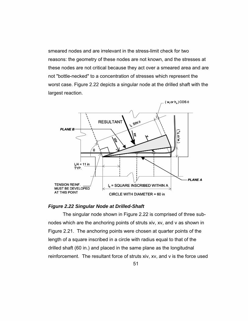
smeared nodes and are irrelevant in the stress-limit check for two
reasons: the geometry of these nodes are not known, and the stresses at
these nodes are not critical because they act over a smeared area and are
not "bottle-necked" to a concentration of stresses which represent the
worst case. Figure 2.22 depicts a singular node at the drilled shaft with the
largest reaction.
lb = SQUARE INSCRIBED WITHIN A
CIRCLE WITH DIAMETER = 60 in
lb/4 = 11 in TYP.
θ
RESULTANT
v
xiv
xv
( wt or ha ) COS θ
l bSIN θ
( wt o
r ha )
TENSION REINF.MUST BE DEVELOPEDAT THIS POINT
PLANE A
PLANE B
lb = SQUARE INSCRIBED WITHIN A
CIRCLE WITH DIAMETER = 60 in
lb/4 = 11 in TYP.
θ
RESULTANT
v
xiv
xv
( wt or ha ) COS θ
l bSIN θ
( wt o
r ha )
TENSION REINF.MUST BE DEVELOPEDAT THIS POINT
PLANE A
PLANE B
Figure 2.22 Singular Node at Drilled-Shaft The singular node shown in Figure 2.22 is comprised of three sub-
nodes which are the anchoring points of struts xiv, xv, and v as shown in
Figure 2.21. The anchoring points were chosen at quarter points of the
length of a square inscribed in a circle with radius equal to that of the
drilled shaft (60 in.) and placed in the same plane as the longitudnal
reinforcement. The resultant force of struts xiv, xv, and v is the force used
51
to calculate the stress acting on the node-strut interface while the reaction
R2 is the force used to calculate the force on the node/drilled-shaft
interface. The geometry of the element and main tension reinforcement is
such that, the hook takes no part in the formation of the geometry of the
node. The radius of the hook lies outside the reaction area so that the
struts frame directly into the drilled shaft and not into the bend radius of
the hook; therefore, the nodal face dimension perpendicular to main
tension reinforcement is given by each code similar to C-C-T nodes
anchoring straight reinforcement. The stress on this face need not be
calculated. This condition may not always be true and should be analyzed
on a case by case basis. The development length of the main tension
reinforcement is taken as the distance behind the point at which the
centroid of tension reinforcement meets the compression strut at node H
in Figure 2.21 and is deemed satisfactory by inspection.
Until this point, the ACI 318-02 and AASHTO LRFD differ only in
load and resistance factors. The treatment of limiting stresses of nodes
and struts by either code authority marks the divergence of provisions by
each.
Applied Stresses
plane A
σ2_AR2
lb2:= σ2_A 1.69ksi=
52

σ2_limit_node_AASHTO 1.89ksi=
σ2_limit_node_AASHTO φ_comp_AASHTO .75⋅ f'c⋅:=
σ2_limit_node_ACI 1.71ksi=σ2_limit_node_ACI φ_comp_AASHTO .85⋅ .8⋅ f'c⋅:=
for C-C-T nodesf'c 3.6 ksi⋅:=φ_comp_AASHTO 0.7:=
ACI 318-02 and AASHTO LRFD Node and Strut Limiting Stresses
σ2_B_AASHTO 1.83ksi=σ2_B_AASHTOresultant_xiv_xv_vws_AASHTO lb⋅
:=
ws_AASHTO lb sin resultant_θ( )⋅ ha cos resultant_θ( )⋅+:=
ha 13.8 in⋅:=
AASHTO LRFD
σ2_B_ACI 1.91ksi=σ2_B_ACIresultant_xiv_xv_v
ws_ACI lb⋅:=
ws_ACI lb sin resultant_θ( )⋅ wt cos resultant_θ( )⋅+:=
wt 9.4 in⋅:=
ACI 318-02
resultant_θ 63 deg⋅:=
resultant_xiv_xv_v 3417 k⋅:=
plane B
NODEw s ACI 318-02 and AASHTO
lb ACI 318-02 and AASHTO
h a A
AS
HTO
wt
AA
SH
TO
53

σ1_A 0.78ksi=σ1_AR1
lb2:=
plane A
APPLIED STRESSES
resultant_θ 48 deg⋅:=
resultant_i_xi 1902 k⋅:=
In a similar manner the stresses at the singular node above reaction 1 are calculated as well as the limiting stresses provide by each code authority.
σ2_limit_strut_AASHTO 1.91ksi=
σ2_limit_strut_AASHTO φ_comp_AASHTO fcu⋅:=
fcuf'c
0.8 170 ε1⋅+:=
ε1 .002 .002 .002+( )1
tan resultant_θ( )2+:=
assuming εs = .002AASHTO LRFD
σ2_limit_strut_ACI_with_reinf 1.61ksi=
σ2_limit_strut_ACI_no_reinf 1.29ksi=
σ2_limit_strut_ACI_with_reinf φ_comp_AASHTO .85⋅ .75⋅ f'c⋅:=
σ2_limit_strut_ACI_no_reinf φ_comp_AASHTO .85⋅ .6⋅ f'c⋅:=
ACI 381-02
Compression Struts
54

σ1_limit_node_AASHTO 1.89ksi=
σ1_limit_node_ACI 1.71ksi=
σ1_limit_node_AASHTO σ2_limit_node_AASHTO:=
σ1_limit_node_ACI σ2_limit_node_ACI:=
for C-C-T nodes the limiting stress remains unchanged
ACI 318-02 and AASHTO LRFD Node and Strut Limiting Stresses
σ1_B_AASHTO 1.1 ksi=σ1_B_AASHTOresultant_i_xi
ws_AASHTO lb⋅:=
ws_AASHTO lb sin resultant_θ( )⋅ ha cos resultant_θ( )⋅+:=
ha 13.8 in⋅:=
AASHTO LRFD
σ1_B_ACI 1.19ksi=σ1_B_ACIresultant_i_xi
ws_ACI lb⋅:=
ws_ACI lb sin resultant_θ( )⋅ wt cos resultant_θ( )⋅+:=
wt 9.4 in⋅:=
ACI 318-02
plane B
55
for compression struts the ACI 318-02provisions are indepent of the angle with respect to the tension tie and remains unchanged
σ1_limit_strut_ACI_no_reinf σ2_limit_strut_ACI_no_reinf:=
σ1_limit_strut_ACI_with_reinf σ2_limit_strut_ACI_with_reinf:=
σ1_limit_strut_ACI_no_reinf 1.29ksi=
σ1_limit_strut_ACI_with_reinf 1.61ksi=
AASHTO LRFD
assuming εs = .002
ε1 .002 .002 .002+( )1
tan resultant_θ( )2+:=
fcuf'c
0.8 170 ε1⋅+:=
σ1_limit_strut_AASHTO φ_comp_AASHTO fcu⋅:= σ1_limit_strut_AASHTO 1.49ksi=
56
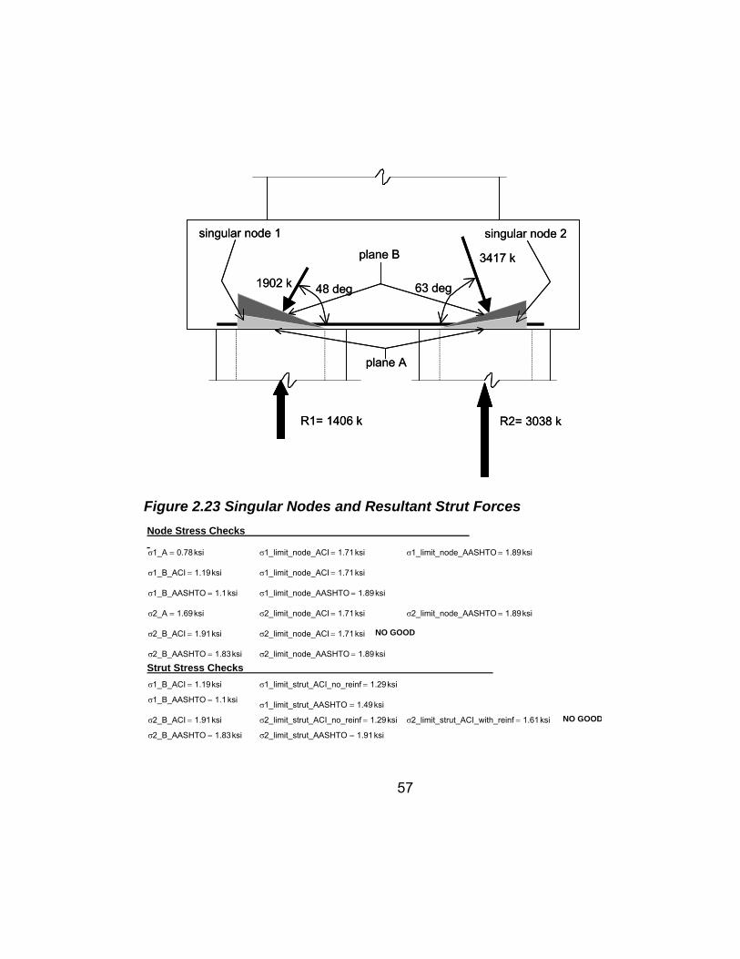
R1= 1406 k
48 deg 63 deg
3417 k
1902 k
R2= 3038 k
singular node 1 singular node 2
plane B
plane A
R1= 1406 k
48 deg 63 deg
3417 k
1902 k
R2= 3038 k
singular node 1 singular node 2
plane B
plane A
Figure 2.23 Singular Nodes and Resultant Strut Forces
σ2_limit_strut_AASHTO 1.91ksi=σ2_B_AASHTO 1.83ksi=
NO GOODσ2_limit_strut_ACI_with_reinf 1.61ksi=σ2_limit_strut_ACI_no_reinf 1.29ksi=σ2_B_ACI 1.91ksi=
σ1_limit_strut_AASHTO 1.49ksi=σ1_B_AASHTO 1.1 ksi=
σ1_limit_strut_ACI_no_reinf 1.29ksi=σ1_B_ACI 1.19ksi=
Strut Stress Checks σ2_limit_node_AASHTO 1.89ksi=σ2_B_AASHTO 1.83ksi=
NO GOODσ2_limit_node_ACI 1.71ksi=σ2_B_ACI 1.91ksi=
σ2_limit_node_AASHTO 1.89ksi=σ2_limit_node_ACI 1.71ksi=σ2_A 1.69ksi=
σ1_limit_node_AASHTO 1.89ksi=σ1_B_AASHTO 1.1 ksi=
σ1_limit_node_ACI 1.71ksi=σ1_B_ACI 1.19ksi=
σ1_limit_node_AASHTO 1.89ksi=σ1_limit_node_ACI 1.71ksi=σ1_A 0.78ksi=
Node Stress Checks
57
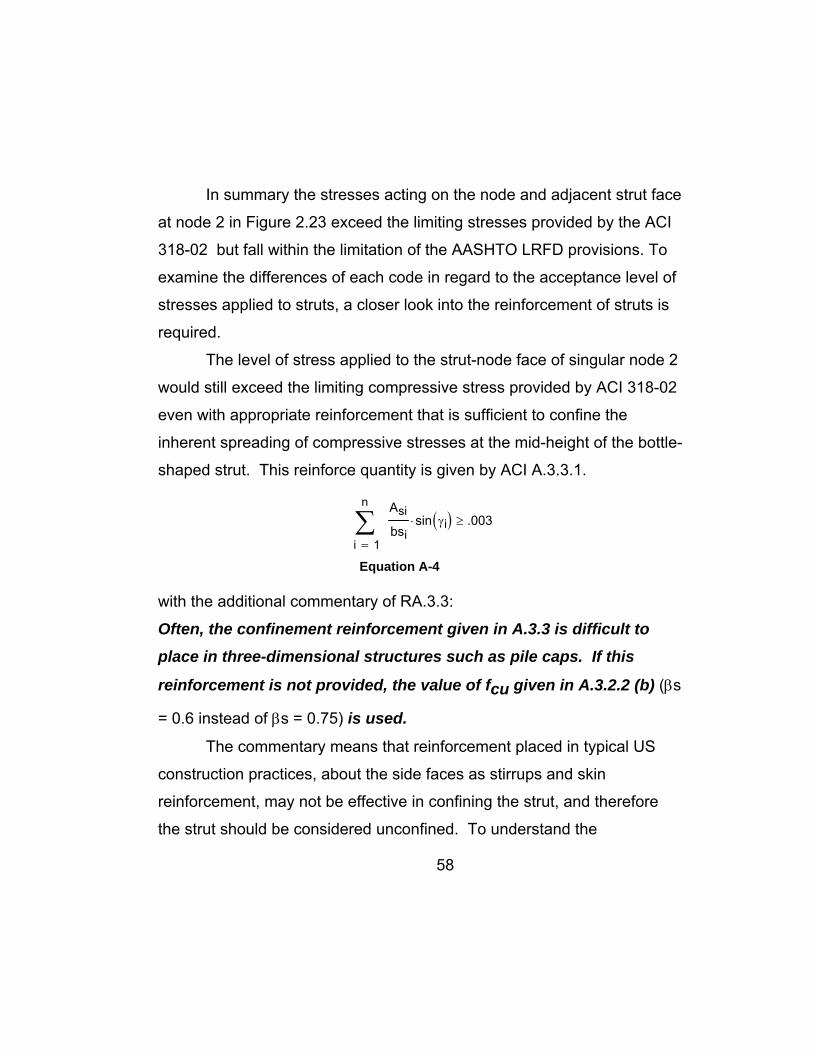
In summary the stresses acting on the node and adjacent strut face
at node 2 in Figure 2.23 exceed the limiting stresses provided by the ACI
318-02 but fall within the limitation of the AASHTO LRFD provisions. To
examine the differences of each code in regard to the acceptance level of
stresses applied to struts, a closer look into the reinforcement of struts is
required.
The level of stress applied to the strut-node face of singular node 2
would still exceed the limiting compressive stress provided by ACI 318-02
even with appropriate reinforcement that is sufficient to confine the
inherent spreading of compressive stresses at the mid-height of the bottle-
shaped strut. This reinforce quantity is given by ACI A.3.3.1.
1
n
i
Asi
bsisin γi( )⋅∑
=
.003≥
Equation A-4
with the additional commentary of RA.3.3:
Often, the confinement reinforcement given in A.3.3 is difficult to
place in three-dimensional structures such as pile caps. If this
reinforcement is not provided, the value of fcu given in A.3.2.2 (b) (βs
= 0.6 instead of βs = 0.75) is used.
The commentary means that reinforcement placed in typical US
construction practices, about the side faces as stirrups and skin
reinforcement, may not be effective in confining the strut, and therefore
the strut should be considered unconfined. To understand the
58

reinforcement needed to confine struts in two or three-dimensional
structures refer to Figure 2.24 and following discussion.
R2
PRESULT
1
2
StrutTie
1
2
StrutTie
3417k
764k
R2
PRESULT
1
2
StrutTie
1
2
StrutTie
3417k
764k
Figure 2.24 Modeling Dispersed Compression Field with 2:1 Bottle-Shaped Strut
To supply the reinforcement required to confine this strut according
to ACI 318-02 the designer may employ equation A-4 or proportion steel
directly based on the 2:1 model which always results in tension = 0.447x
compression. The following sample calculation displays how the quantity
of confining steel may be computed using equation A-4 or the 2:1 model
for spread of compressive stresses.
59
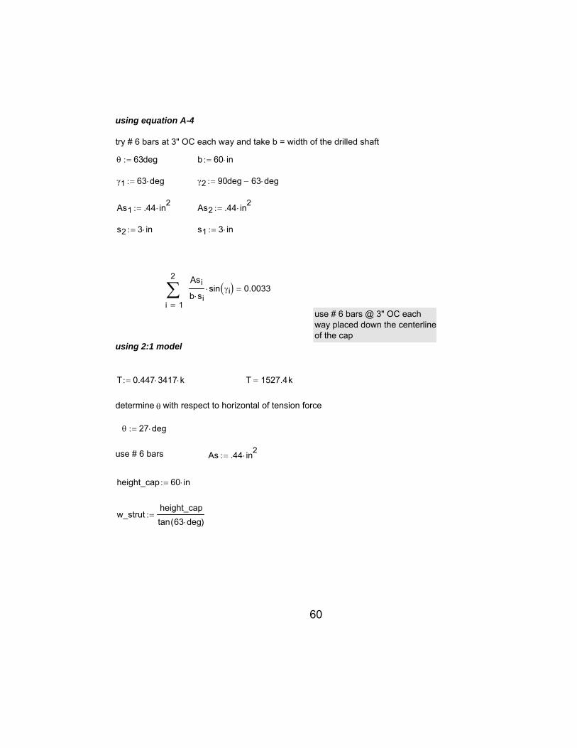
w_strutheight_captan 63 deg⋅( )
:=
height_cap 60 in⋅:=
As .44 in2⋅:=use # 6 bars
θ 27 deg⋅:=
determine θ with respect to horizontal of tension force
T 1527.4k=T 0.447 3417⋅ k⋅:=
using 2:1 model
use # 6 bars @ 3" OC eachway placed down the centerlineof the cap
1
2
i
Asi
b si⋅sin γi( )⋅∑
=
0.0033=
s1 3 in⋅:=s2 3 in⋅:=
As2 .44 in2⋅:=As1 .44 in2
⋅:=
γ2 90deg 63 deg⋅−:=γ1 63 deg⋅:=
b 60 in⋅:=θ 63deg:=
try # 6 bars at 3" OC each way and take b = width of the drilled shaft
using equation A-4
60
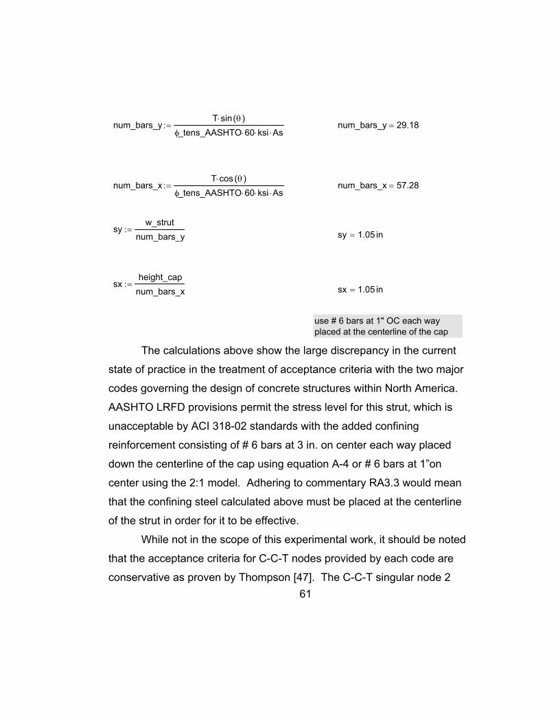
num_bars_yT sin θ( )⋅
φ_tens_AASHTO 60⋅ ksi⋅ As⋅:= num_bars_y 29.18=
num_bars_xT cos θ( )⋅
φ_tens_AASHTO 60⋅ ksi⋅ As⋅:= num_bars_x 57.28=
syw_strut
num_bars_y:= sy 1.05 in=
sxheight_cap
num_bars_x:= sx 1.05 in=
use # 6 bars at 1" OC each way placed at the centerline of the cap
The calculations above show the large discrepancy in the current
state of practice in the treatment of acceptance criteria with the two major
codes governing the design of concrete structures within North America.
AASHTO LRFD provisions permit the stress level for this strut, which is
unacceptable by ACI 318-02 standards with the added confining
reinforcement consisting of # 6 bars at 3 in. on center each way placed
down the centerline of the cap using equation A-4 or # 6 bars at 1”on
center using the 2:1 model. Adhering to commentary RA3.3 would mean
that the confining steel calculated above must be placed at the centerline
of the strut in order for it to be effective.
While not in the scope of this experimental work, it should be noted
that the acceptance criteria for C-C-T nodes provided by each code are
conservative as proven by Thompson [47]. The C-C-T singular node 2
61
62
exceeded the stress limit provided by ACI; however, this node as well as
node 1 is bi-axially confined as with any node whose bearing dimension is
smaller than that of the surrounding concrete.
Although every stress level was acceptable by AASHTO LRFD
standards, the same stress level exceeded ACI 318-02 standards leaving
the designer unsure and uncomfortable about a final design acceptable by
only one standard. It would be desirable to have agreement on the same
method and achieve a consistent design standard regardless of the
method being used in bridge or building structures. Finally the strut-and-
tie method produced an equivalent amount of main tension reinforcement
as that originally calculated by TxDOT engineers using an allowable stress
criterion with pure bending theory. The vertical tension reinforcement
calculated by the strut-and tie method is twice that provided by TxDOT
engineers who discerned that shear is not a factor; however the tie
reinforcement was placed as good practice. The strut-and-tie model
shows shear forced at the lightly loaded drilled-shaft and the
reinforcement proportioned for shear at that location is placed the entire
length as good practice.
Figure 2.25 shows the comparison of amounts of reinforcement
required by the strut-and-tie model shown in Figure 2.21 in the two
orthogonal dimensions of the drilled-shaft cap omitting skin reinforcement,
temperature and shrinkage reinforcement, and "feel good reinforcement"
as called for by original TxDOT calculations.

18 # 1118 # 11
Figure 2.25 Comparison of Drilled-Shaft Cap Reinforcement Resulting from TxDOT and STM Analyses
63
64
3.0 EXPERIMENTAL PROGRAM
3.1 GENERAL
The experimental program consisted of a series of laboratory
experiments designed to investigate the behavior of bottle-shaped struts.
Twenty-eight tests were conducted in three basic series. The design of
each series was a progressive process in which data from the first series
was analyzed to determine appropriate parameters and to improve the
next series in order to isolate the parameters influencing strut behavior.
3.2 TEST SET-UP
The test set-up is analogous to split-cylinder testing in which
monotonic load is applied at an increasing rate to a specimen whose
geometry and orientation allow for the dispersion of compression and
associated transverse tension to develop within the boundary of the
specimen. In this case, load was applied by a universal testing machine
(UTM) to square or rectangular, unreinforced, and reinforced concrete
panels through steel bearing plates. The dimensions of the bearing plates
were significantly less than the surface area of concrete at the loaded
ends. The basic test set-up is shown in Figure 3.1. To ensure that the
force from the loading head of the UTM was applied to the concrete
surface uniformly; hydrostone was placed at the concrete-steel plate
interface, as well as, a spherical head placed at the plate-loading head
interface. The specimens were plumbed before testing to ensure
alignment. Strain measurements were collected through series of electric
strain gauges applied to the reinforcement within the specimens and the

concrete surface of the specimens. (Instrumentation will be discussed in
detail in subsequent sections) The strain measurements were recorded
through data-acquisition hardware and software available at the Ferguson
Structural Engineering Laboratory at the University of Texas at Austin.
Load was recorded through the same data-acquisition systems in parallel
with internal load cells within the universal testing machine. Displacement
recordings were not taken in light of Sanders’ [44] and Wollman’s [51]
experimentation in which they concluded that isolated specimens such as
these failed in a non-ductile manner providing little or no useful load-
displacement data.
Figure 3.1 Typical Test Set-Up
65

66
3.3.2.1
3.3 SERIES 1 SPECIMENS
3.3.1 General
The first series of specimens consisted of 6 specimens from two
batches of concrete. This series consisted of 3 ft. by 3 ft. by 4 in. thick
reinforced and unreinforced concrete panels, and the main foci of this
series was to achieve an optimal system of instrumentation, and to
substantiate the choice of the overall specimen geometry. Therefore,
different arrangements of instrumentation were used. The patterns of
reinforcement varied as well. All specimens were tested using 4 in by 12
in. by 2 in. bearing plates defining the nodal area, and reinforced with
orthogonal mats of reinforcement consisting of #3 bars. From this point
forward specimens will be designated thus: S#-# with S# referring to
series 1, 2 or 3, and the last number represents the order tested within the
series.
3.3.2 Specimen S1-1
Instrumentation
At the outset of the experimental program, it was the original goal of
the research team to obtain the principle stresses at points evenly dividing
one quadrant of a specimen. For this reason a specimen S1-1 was
fabricated to include embedded strain rosettes. These rosettes were
fabricated from thin gauge sheet metal having three axes at 0 deg., 45
deg., and 90 deg. The anchoring points were established at the end of
each axis by brazing a sheet-metal screw to the rosette through a pre-
fabricated hole. The rosettes were then gauged with electronic strain

gauges placed at the center of each leg forming the three axes and
debonded from the concrete by placing HVAC foil-tape around each axis
leaving only the anchorage points exposed. 6 in. and 2 in. axis lengths
were investigated. The rosettes tied to the reinforcing cage are shown in
Figure 3.2.
Figure 3.2 Embedded Strain Rosettes.
The reinforcing cage was also instrumented with electronic strain
gauges at one quadrant of the specimen on every reinforcing bar at 3 in.
from the form face and 6 in. on center until the specimen’s centerline was
reached.
67

68
3.3.2.2 S1-1 Behavior
The specimen behavior is briefly described here and in the
following sections, because as stated previously, the experimental
program was an evolving process in which each series of specimen were
designed based on knowledge compounding from earlier testing.
At first appearance, S1-1 seemed to have failed within the nodal
region, such a failure was undesirable since the behavior of bottle-shaped
struts was anticipated and thought to have failures typified by large cracks
at the specimen centerline. Figure 3.3 shows the failure mode of
specimen S1-1 which can be visually described by slight spalling of the
nodal region and one hairline crack down the centerline of the specimen.
Figure 3.3 Failure Mode of Specimen S1-1
When the data gathered from the embedded rosettes was
analyzed, the accuracy of the results to capture the specimen’s behavior
was questionable and inconsistent. The research team subsequently
abandoned further use of the embedded rosette.

69
3.3.3.1
3.3.3 Specimens S1-2, S1-3, S1-4, S1-5, S1-6
Specimen S1-2 Instrumentation
Adhering to the idea of obtaining the principle stress at points
evenly dividing one quadrant of a specimen; embedded rosettes were
replaced with surface rosettes for this specimen. Two styles of surface
rosettes were investigated with specimen S1-2: The first style was a
prefabricated surface rosette that had no lead wires requiring that wire be
soldered to the gauge before testing could take place which proved to be
a lengthy and unreliable process. The second style of rosette consisted of
3 – 60mm. long surface gauges (referred hereafter as 2 in. surface
gauges) applied directly over each other at three axes of 0 deg., 45 deg.,
and 90 deg. The two styles of rosettes were oriented on specimens S1-2
as shown in Figure 3.4 with the hope of capturing the 2:1 spread of
compression stresses as reported by Burdet [17] and to assess what type
of rosette best captured this behavior. Single surface gauges were also
placed on the centerline transverse axis in order to integrate the strains
over the area of the specimen and compare that calculation with the load
applied. If these values agreed reasonably well, an evaluation of the
adequacy surface gauges in capturing the behavior of the specimen in
compression could be made. Figure 3.4 also demonstrates how surface
gauges were applied to each specimen.

70
3.3.3.2 Specimen S1-2 Behavior
Specimen S1-2 was unreinforced to ensure that reinforcement did
not restrain the elastic 2:1 spread of compression and therefore no
comparisons could be made from strain readings taken from
TRANSVERSE AXIS
2 in singular surface gaugespre-fabricated rosettes
LOA
D A
XIS
exterior surface ground smooth removing surface paste
2-part epoxy ground to seal surface only
typical 2 in. surface strain gauge
TRANSVERSE AXIS
2 in singular surface gaugespre-fabricated rosettes
LOA
D A
XIS
exterior surface ground smooth removing surface paste
2-part epoxy ground to seal surface only
typical 2 in. surface strain gauge
2 in singular surface gaugespre-fabricated rosettes
LOA
D A
XIS
exterior surface ground smooth removing surface paste
2-part epoxy ground to seal surface only
typical 2 in. surface strain gauge
Figure 3.4 Specimen S1-2 Surface Gauge Instrumentation reinforcement gauges in specimen S1-1. The pre-fabricated and built-up
rosettes compared well with each other and did capture the principle
strains at angles ranging from 22 deg. to 27 deg. In light of these finding
built-up rosettes were chosen for placement on the surface of specimens
S2-2, S2-3, S2-4, and S2-5 due to ease of application. Furthermore, the
strain gauges placed at the transverse axis captured the load when
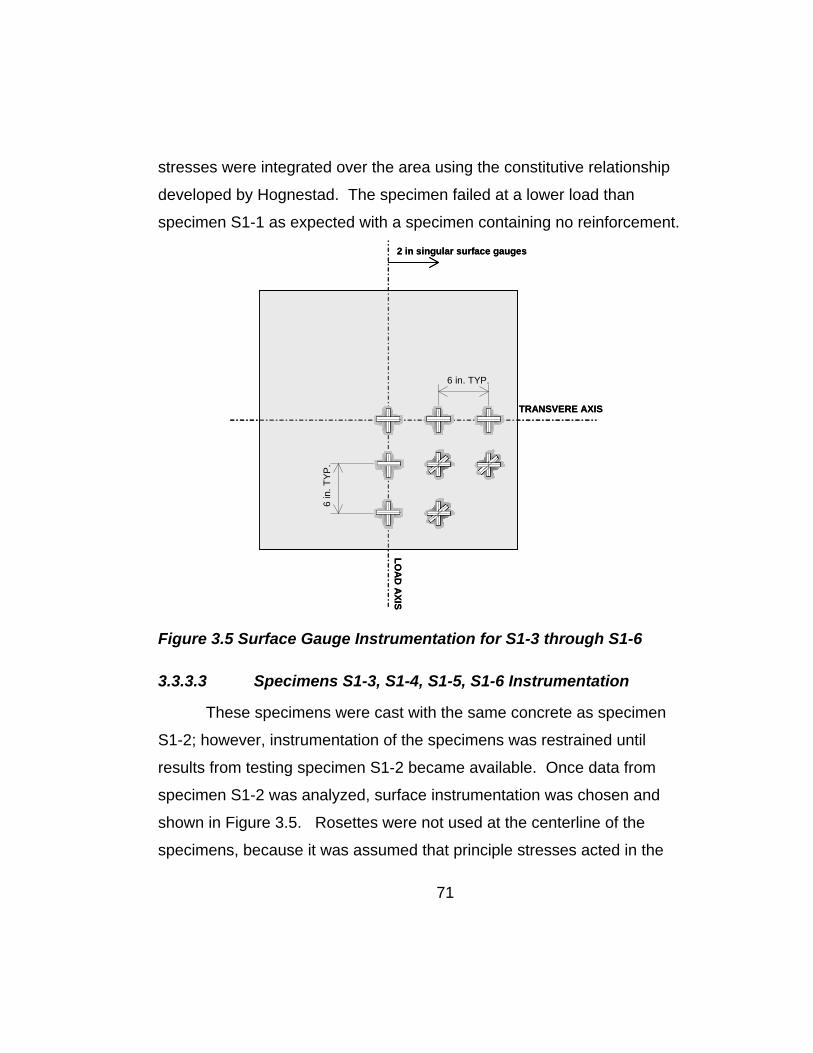
stresses were integrated over the area using the constitutive relationship
developed by Hognestad. The specimen failed at a lower load than
specimen S1-1 as expected with a specimen containing no reinforcement.
2 in singular surface gauges
LOA
D A
XIS
6 in
. TYP
.
6 in. TYP.
TRANSVERE AXIS
2 in singular surface gauges
LOA
D A
XIS
6 in
. TYP
.
6 in. TYP.
TRANSVERE AXIS
Figure 3.5 Surface Gauge Instrumentation for S1-3 through S1-6
3.3.3.3 Specimens S1-3, S1-4, S1-5, S1-6 Instrumentation
These specimens were cast with the same concrete as specimen
S1-2; however, instrumentation of the specimens was restrained until
results from testing specimen S1-2 became available. Once data from
specimen S1-2 was analyzed, surface instrumentation was chosen and
shown in Figure 3.5. Rosettes were not used at the centerline of the
specimens, because it was assumed that principle stresses acted in the
71

orthogonal directions of the specimen at theses locations. All surface
gauges were applied as shown in Figure 3.4, and only built-up rosettes
consisting of 2 in surface gauges were used.
Specimens S1-3 and S1-4 contained only the instrumentation
shown in Figure 3.5. Specimens S1-5 and S1-6 contained orthogonal
mats of reinforcement and were instrumented with reinforcement gauges
at the locations were the vertical and horizontal bars met in one quadrant
of the specimen.
72
3.3.3.4 Specimens S1-3, S1-4 and S1-5 Special Reinforcing
In order to investigate the role of the node at the point where load
was applied in these specimens and to force failure away from the node;
special confining reinforcement was placed in specimens S1-3, S1-4, and
S1-5. The confining reinforcement consisted of either 2 or 3 closed ties
encompassing 6 vertical bars welded to a bearing plate as seen in Figure
3.6 shown in the form before casting.
A) Confining Reinforcement at Nodesfor Specimens S1-3, S1-6
B) Confining Reinforcement at Nodesfor Specimen S1-4
A) Confining Reinforcement at Nodesfor Specimens S1-3, S1-6
B) Confining Reinforcement at Nodesfor Specimen S1-4
Figure 3.6 Confining Reinforcement for Nodes

73
3.3.3.5 Specimens S1-3 through S1-6 Behavior
Specimens S1-3 and S1-4 were identical to specimen S-1 having
no orthogonal reinforcement; however as stated above S1-3 and S1-4 had
different levels of confining reinforcement at the node location. Specimen
S1-5 was identical to specimen S1-1 in regard to orthogonal
reinforcement, but also had the confining reinforcement at the node
locations shown in Figure 3.6 A). The specimens whose nodes were
confined displayed no particular behavior in respect to cracking patterns or
modes of failure different from specimens whose nodes were unconfined
other than the ultimate loads when normalized with respect to the differing
concrete strengths were around two times that of the unconfined
specimens. Furthermore, when removing crushed concrete around the
node of specimens S1-6 a clearly defined area of the node could be seen
in which the mode of failure was strut crushing at the node-strut interface.
These two observations determined that further confinement of the node
was not necessary to achieve the desired behavior of bottle-shaped struts. tensile crack
crushing of the strutat the node-strut interface
NODE
STRU
TSTRUT
tensile crack
crushing of the strutat the node-strut interface
NODE
STRU
TSTRUT
Figure 3.7 Crushing of the Strut at the Node-Strut Interface, S1-6
74
A detailed description of the specimen dimensions, bearing plate
dimensions, amount of reinforcement, atypical loading conditions (if any),
and material properties for this series of specimens as well as every other
specimen tested within the experimental program can be seen in Figures
3.12 through 3.15 and Tables 3.1 through 3.3 at the end of this chapter.
3.4 SERIES 2 SPECIMENS
3.4.1 General
Confident that the overall specimen geometry was sufficient to
study the behavior of bottle-shaped struts based on the observations seen
in the first series of specimens; Series 2 specimens were designed as 3 ft.
by 3 ft by 6 in thick concrete panels with no nodal confinement with a
particular regime of reinforcement and instrumentation. All specimens
were cast together, yet 3 cylinders were tested each day testing occurred
in order to have specific values of concrete strength for each specimen.
All specimens were tested using 6 in. by 12 in. by 2 in. bearing plates
defining the nodal area and reinforced with #2 or # 3 reinforcing bars.
3.4.2 Series 2 Instrumentation
The surface rosettes were abandoned in the Series 2 specimens
because the data provided from the Series 1 tests was not valuable
enough to warrant the time and effort spent in the application of these
gauges. Rather, five surface gauges were applied to each specimen at
the transverse axis to one side of the specimen shown in Figure 3.8 A.
The exception to this pattern occurred wherever a reinforcing bar parallel
to the load axis was present, in which case, a surface gauge was located
75
at the transverse axis at the point of the reinforcing bar beneath as
illustrated in Figure 3.8 B. This measure was taken to compare the strain
measurements recorded on the concrete surface with the strain
measurements taken internally.
Strain gauges were also placed on reinforcement within the
specimens at the point in which the reinforcement crossed the load axis or
transverse axis. This instrumentation was usually restricted to
reinforcement placed to one side of the load axis dividing the specimen in
half; however, as with the surface gauges, reinforcement gauges were
occasionally placed symmetrically about the load axis to verify the
distribution of stress across the specimen.

TRANSVERSE AXIS
2 in. singular surface gauges
LOA
D A
XIS
4 in. TYP.
occasional straingauge to verifyeven distributionof stress
TRANSVERSE AXIS
2 in. singular surface gauges
LOA
D A
XIS
4 in. TYP.
occasional straingauge to verifyeven distributionof stress
TRANSVERSE AXIS
2 in. singular surface gauges
LOA
D A
XIS
4 in. T.Y.P UNO
DIM to matchReinf. location
TRANSVERSE AXIS
2 in. singular surface gauges
LOA
D A
XIS
4 in. T.Y.P UNO
DIM to matchReinf. location
A) Typical Series 2 Specimen Surface Gauge Location
B) Series 2 Specimen Surface Exception
TRANSVERSE AXIS
2 in. singular surface gauges
LOA
D A
XIS
4 in. TYP.
occasional straingauge to verifyeven distributionof stress
TRANSVERSE AXIS
2 in. singular surface gauges
LOA
D A
XIS
4 in. TYP.
occasional straingauge to verifyeven distributionof stress
TRANSVERSE AXIS
2 in. singular surface gauges
LOA
D A
XIS
4 in. T.Y.P UNO
DIM to matchReinf. location
TRANSVERSE AXIS
2 in. singular surface gauges
LOA
D A
XIS
4 in. T.Y.P UNO
DIM to matchReinf. location
A) Typical Series 2 Specimen Surface Gauge Location
B) Series 2 Specimen Surface Exception
Figure 3.8 Series 2 Surface Gauge Instrumentation
76
77
3.4.3 Series 2 Reinforcement
The only provisions available for the reinforcement of bottle-shaped
struts is given in ACI 318-02 A.3.3.1 (presented in 1.2.3 of this thesis) or
reinforcement proportioned using the 2:1 model (also presented in that
section). In order to investigate the adequacy of the relevant ACI
provisions, specimens included reinforcement ratios on the order of 0.5,
1.0, and 1.5 times the amount reinforcement given in ACI equation A-4
which is presented as a reinforcement ratio. To satisfy these ratios U.S.
#3 bars were used as well as #2 (6mm) bars. These bars were typically
placed in orthogonal mats symmetric about the load axis and transverse
axis and at mid-depth of the thickness dimension. Other variables
regarding the reinforcement of the specimens included the orientation of
the orthogonal mats with respect to the load axis of the specimen to
simulate struts crossing reinforcement at an angle, as well as, the
distribution of reinforcement (lumped versus evenly distributed). The
variables involved in the reinforcement of the specimens in Series 2 are
shown graphically in Figure 3.9.
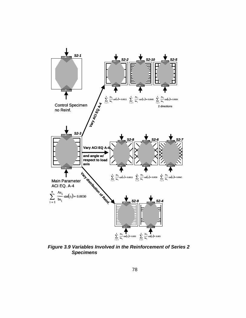
1i = 1i =
Control Specimenno Reinf.
1
n
i
As i
bsisin γi( )⋅∑
=
0.00151
n
i
Asi
bsisin γi( )⋅∑
=
0.0045
S2-1S2-2 S2-10 S2-5
Vary
ACI
EQ
A-4
Main ParameterACI EQ. A-4
S2-3
S2-8 S2-6 S2-7
Vary ACI EQ A-4
and angle w/respect to loadaxis
n As i
bsisin γi( )⋅∑ 0.003
n As i
bsisin γi( )⋅∑ 0.003
Vary distribution of Reinf. S2-9 S2-4
1
n
i
As i
bsisin γi( )⋅∑
=
0.00151
n
i
As i
bs isin γ i( )⋅∑
=
0.0045
1
n
i
Asi
bsisin γi( )⋅∑
=
0.0030
1
n
i
Asi
bsisin γi( )⋅∑
=
0.0030
1
n
i
Asi
bsisin γi( )⋅∑
=
0.0030
2 directions
Figure 3.9 Variables Involved in the Reinforcement of Series 2 Specimens
78
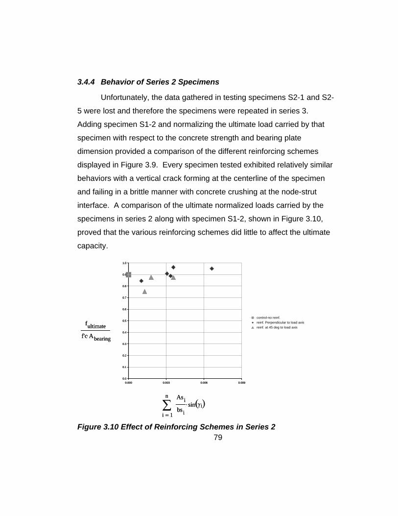
3.4.4 Behavior of Series 2 Specimens
Unfortunately, the data gathered in testing specimens S2-1 and S2-
5 were lost and therefore the specimens were repeated in series 3.
Adding specimen S1-2 and normalizing the ultimate load carried by that
specimen with respect to the concrete strength and bearing plate
dimension provided a comparison of the different reinforcing schemes
displayed in Figure 3.9. Every specimen tested exhibited relatively similar
behaviors with a vertical crack forming at the centerline of the specimen
and failing in a brittle manner with concrete crushing at the node-strut
interface. A comparison of the ultimate normalized loads carried by the
specimens in series 2 along with specimen S1-2, shown in Figure 3.10,
proved that the various reinforcing schemes did little to affect the ultimate
capacity.
1
n
i
Asi
bsisin γi( )⋅∑
=
fultimate
f'c Abearing⋅
0.0
0.1
0.2
0.3
0.4
0.5
0.6
0.7
0.8
0.9
1.0
0.000 0.003 0.006 0.009
control-no reinf.reinf. Perpendicular to load axisreinf. at 45 deg to load axis
1
n
i
Asi
bsisin γi( )⋅∑
=
fultimate
f'c Abearing⋅
0.0
0.1
0.2
0.3
0.4
0.5
0.6
0.7
0.8
0.9
1.0
0.000 0.003 0.006 0.009
control-no reinf.reinf. Perpendicular to load axisreinf. at 45 deg to load axis
79Figure 3.10 Effect of Reinforcing Schemes in Series 2
80
3.5 SERIES 3 SPECIMENS
3.5.1 General
The effects of various reinforcement distributions shown in Figure
3.10 proved that amount, distribution, and reinforcement angle with
respect to the load axis of the specimen had little effect on the overall
behavior. For this reason series 3 specimens were designed to vary the
boundary conditions of the basic specimen in order to produce more
dramatic changes to the overall behavior. Two specimens, S3-1 and S3-
5, were replicates of specimens S2-1 and S2-5 because the data gathered
in testing these two specimens were lost as mentioned previously.
3.5.2 Series 3 Instrumentation
The instrumentation regime presented in 3.4.2 was used in the
Series 3 specimens because it provided the data needed to understand
the behavior of specimens and allowed direct comparisons between
Series 1 and 2.
3.5.3 Reinforcement Patterns Used in Series 3 Specimens
Generally, the specimens within series 3 were reinforced with an
amount of reinforcement stipulated by ACI equation A-4; however
specimens S3-2 and S3-6 were reinforced differently with specimen S3-2
testing the practical minimum amount reinforcement for these specimens
containing only one #3 bar located at the transverse axis, and specimen
S3-6 reinforced with 4 # 3’s oriented parallel to the load axis under the
bearing surface, and 3 # 3 bars at third points oriented parallel to the
transverse axis. Specimen S3-7 contained lumped reinforcement in the

81
same quantity as S2-4 but spaced farther apart from the specimen’s
transverse axis. S3-8 reinforcement was placed in an orthogonal mat at
angles of 30 deg and 60 deg relative to the load axis of the specimen. The
reinforcement of specimens S3-9 and S3-10 was placed near the form
face and finished face in two mats (previous specimens all had
reinforcement placed at mid-depth of the 4 or 6 in. dimension). The
reinforcement of specimens S3-3, S3-4, S3-11, S3-12 all had the same
amount of reinforcement as S2-3, but varied in boundary conditions as
discussed in the following section. These reinforcing schemes
represented variables not investigated in the series 2 specimens.
dimension). These reinforcing schemes represented variables not
investigated in the series 2 specimens
3.5.4 Series 3 Boundary Conditions
As stated previously, the boundary conditions varied within this
series with S3-3, S3-4, and S3-7 through S3-12 having different boundary
conditions than the typical specimen of series 2. The standard bearing
plate dimensions of 6 in. by 12 in. by 2 in. in series 2 was changed to 6 in
by 6 in by 2 in is testing specimens S3-4, S3-7, and S3-8. The standard
bearing plate configuration of the series 2 specimen was changed to allow
shear deformations and eliminate horizontal friction in specimen S3-3 as
shown in Figure 3.11. Specimens S3-9 and S3-10 were formed to have a
thickness of 10 in. rather than the standard 6 in. and were tested using 4
in by 12 in. by 2 in. bearing plates placed at the center of the plan area of
the specimens. Specimens S3-11 and S3-12 were cast having the
standard height of 36 in. and depth of 6 in. but the width of these
82
specimens was changed to 60 in, and S3-11 was tested using the
standard bearing plate dimensions while specimenS3-12 was tested using
a larger bearing plate having the dimensions of 6 in. by 16 in. by 3 in. The
specific details of these specimens along with every specimen tested will
be summarized in 3.6.
3.5.5 Behavior of Series 3 Specimens
The qualitative behavior of the specimens tested in series 3 was
similar to all other specimens tested with the failure mode beginning as a
hairline crack parallel to the load axis of the specimen and gradually
widening until an ultimate non-ductile failure categorized by crushing of
the concrete at the node-strut interface prevented any further load being
sustained by the specimen.
The data gathered from the electronic instrumentation placed within
this series as well as all other data gathered from all the previous
specimens, when analyzed, proved that no further testing was required
and ended the experimental program after series 3 testing. The complete
data gathered from all specimens will be presented in Chapter 4 and
analyzed with commentary in Chapter 5.

rigid surfacespherical head orUTS loading platform
specimen surface
hydrostone6 in x 12 in x 2 inbearing plate
2- 6 in x 5-7/8 in x 2 inbearing plates
¾ stiff neoprene pad
12 in. 12 in.
Standard Bearing PlateConfiguration
Modified Bearing PlateConfiguration for S3-3
rigid surfacespherical head orUTS loading platform
specimen surface
hydrostone6 in x 12 in x 2 inbearing plate
2- 6 in x 5-7/8 in x 2 inbearing plates
¾ stiff neoprene pad
12 in. 12 in.
Standard Bearing PlateConfiguration
Modified Bearing PlateConfiguration for S3-3
Figure 3.11 Modified Bearing Plate Configuration
3.6 SPECIMEN SUMMARY
A complete summary of the contents and configuration of every
specimen tested is described in Table 3.1. Figure 3.12 illustrates a typical
specimen elevation for use with Table 3.1. Figure 3.13, Figure 3.14, and
Figure 3.15 following Table 3.1 further illustrate specific reinforcement
placement, non-standard conditions, or further explanation of the material
presented in that table. The material properties used in the fabrication of
each specimen include the yield strain and the modulus of elasticity for the
reinforcing steel listed in Table 3.2, the tensile strength of concrete listed
in Table 3.3, and the compressive strength of concrete is listed in Table
3.1. The compressive strength of concrete was tested each day a
specimen was tested while the tensile strength of concrete was tested
after the complete testing of one series of specimen.
83

BA
LL S
PEC
IMEN
S 36
in.
PL TOP
PL BOT
2
1
TRANSVERSE AXIIS
LOA
D A
XIIS
ρV = As/(BT)
T
T/2
B
1SECTION
ρh = As/(36T)
TT/2
36 in.
2SECTION
MATT TYPEC FROM FIGURE3.13 (interior)
BA
LL S
PEC
IMEN
S 36
in.
PL TOP
PL BOT
2
1
TRANSVERSE AXIIS
LOA
D A
XIIS
ρV = As/(BT)
T
T/2
B
ρV = As/(BT)
T
T/2
B
1SECTION
1SECTION
ρh = As/(36T)
TT/2
36 in.
2SECTION
2SECTION
MATT TYPEC FROM FIGURE3.13 (interior)
Figure 3.12 Typical Specimen Elevation for Use with Table 3.1
84
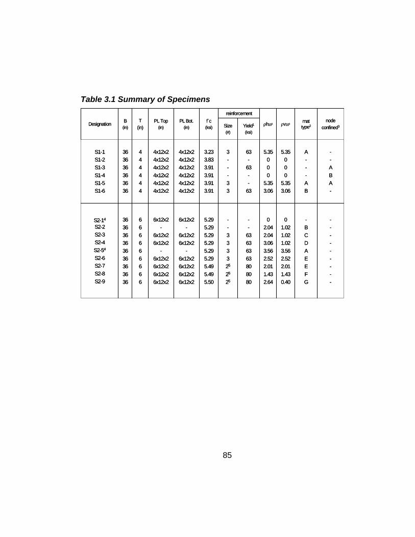
Table 3.1 Summary of Specimens
--
63636363808080
63-
63--
63
Size(#)
Yield1
(ksi)
---------
-BCDAEEFG
01.021.021.023.562.522.011.430.40
02.042.043.063.562.522.011.432.64
--333325
25
25
5.295.295.295.295.295.295.495.495.50
6x12x2-
6x12x26x12x2
-6x12x26x12x26x12x26x12x2
6x12x2-
6x12x26x12x2
-6x12x26x12x26x12x26x12x2
666666666
363636363636363636
S2-14
S2-2S2-3S2-4S2-54
S2-6S2-7S2-8S2-9
--ABA-
A---AB
5.35000
5.353.06
5.35000
5.353.06
3---33
3.233.833.913.913.913.91
4x12x24x12x24x12x24x12x24x12x24x12x2
4x12x24x12x24x12x24x12x24x12x24x12x2
444444
363636363636
S1-1S1-2S1-3S1-4S1-5S1-6
nodeconfined3
mat type2ρv103ρh103
reinforcementf`c(ksi)
PL Bot.(in)
PL Top(in)
T(in)
B(in)
Designation
85

Table 3.1 Continued Summary of Specimens
-6363636363636363
80/636363
63
Size(#)
Yield1
(ksi)
--------XX--
-HCCAIJ
--LL
00
1.021.023.562.041.023.481.221.220.610.61
00.513.563.563.561.533.063.483.063.063.563.56
-33333333
25/333
4.204.204.304.304.304.354.354.354.354.354.354.35
6x12x26x12x2
2-6x6x26
2-6x6x26x12x26x12x26x12x26x6x24x12x24x12x26x16x26x12x3
6x12x26x12x2
2-6x6x26
6x6x26x12x26x12x26x6x26x6x24x12x24x12x26x16x26x12x3
66666666101066
363636363636363636366060
S3-1S3-2S3-3S3-47
S3-5S3-6S3-7S3-8S3-98
S3-108
S3-11S3-12
-G1.026.6235.506x12x26x12x2636S2-10
nodeconfined3
mat type2ρv103ρh103
reinforcementf`c(ksi)
PL Bot.(in)
PL Top(in)
T(in)
B(in)
Designation
1Nominal yield stress2 Letter corresponds to mat types in Figure 3.133 A or B corresponds to Figure 3.6 X indicates node confined by surrounding concrete
4 Data lost during testing5 #2 bars are 6mm diameter Mexican manufactured bars
6 Modified bearing plate configuration seen in Figure 3.117 Refer to Figure 3.14for testing conditions8 Refer to Figure 3.15for complete details of specimen
86
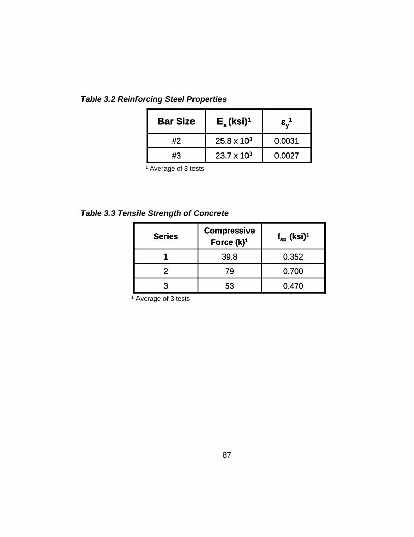
Table 3.2 Reinforcing Steel Properties
0.002723.7 x 103#3
0.003125.8 x 103 #2
εy1Es (ksi)1Bar Size
0.002723.7 x 103#3
0.003125.8 x 103 #2
εy1Es (ksi)1Bar Size
1 Average of 3 tests
Table 3.3 Tensile Strength of Concrete
0.470533
0.70079 2
0.35239.81
fsp (ksi)1CompressiveForce (k)1Series
0.470533
0.70079 2
0.35239.81
fsp (ksi)1CompressiveForce (k)1Series
1 Average of 3 tests
87
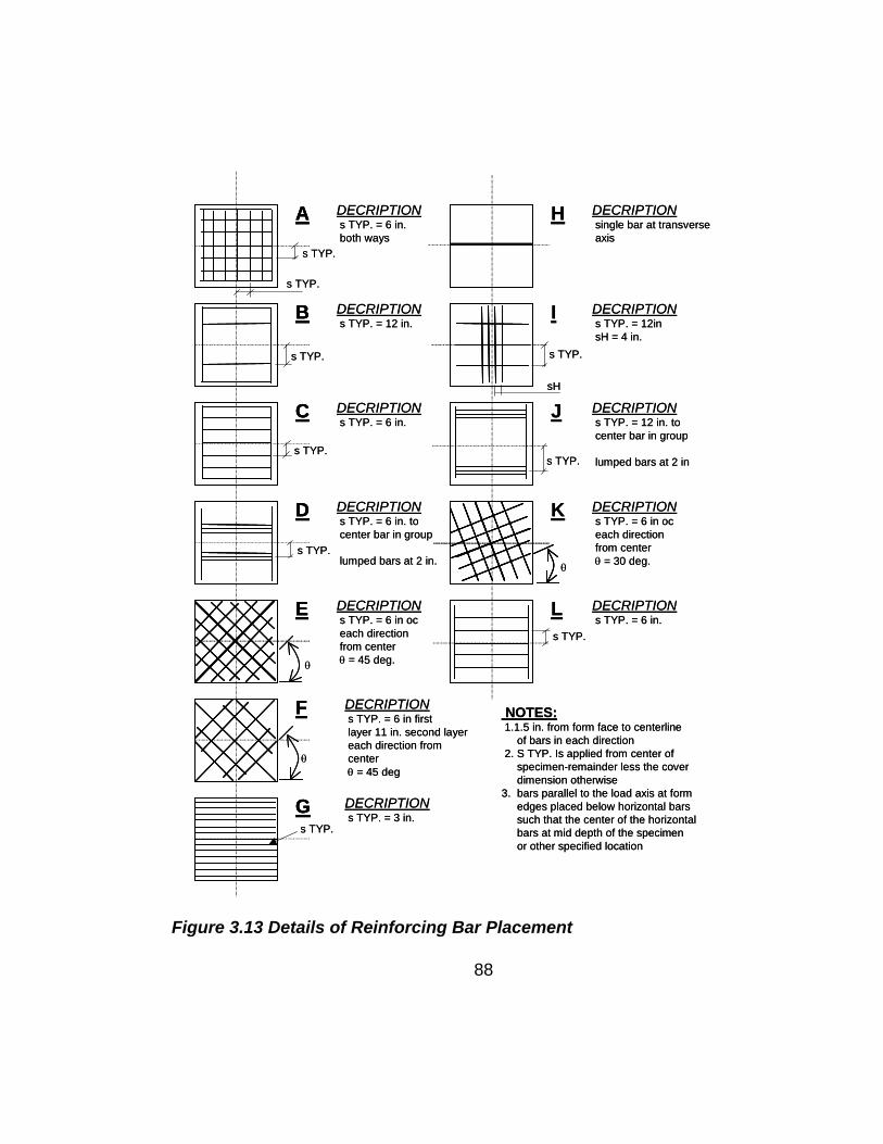
A
B
C
D
E
F
G
H
I
J
K
L
s TYP.
s TYP.
s TYP.
s TYP.
s TYP.
s TYP.
s TYP.
sH
s TYP.
s TYP.
θ
θ
θ
DECRIPTIONs TYP. = 6 in.both ways
DECRIPTIONs TYP. = 12 in.
DECRIPTIONs TYP. = 6 in.
DECRIPTIONs TYP. = 12 in. tocenter bar in group
lumped bars at 2 in
DECRIPTIONs TYP. = 6 in. tocenter bar in group
lumped bars at 2 in.
DECRIPTIONs TYP. = 6 in oceach directionfrom center θ = 30 deg.
DECRIPTIONs TYP. = 6 in oceach directionfrom center θ = 45 deg.
DECRIPTIONs TYP. = 6 in.
DECRIPTIONs TYP. = 6 in firstlayer 11 in. second layereach direction fromcenterθ = 45 deg
DECRIPTIONs TYP. = 3 in.
DECRIPTIONs TYP. = 12insH = 4 in.
DECRIPTIONsingle bar at transverseaxis
NOTES: 1.1.5 in. from form face to centerline
of bars in each direction2. S TYP. Is applied from center of
specimen-remainder less the cover dimension otherwise
3. bars parallel to the load axis at formedges placed below horizontal barssuch that the center of the horizontalbars at mid depth of the specimenor other specified location
A
B
C
D
E
F
G
A
B
C
D
E
F
G
H
I
J
K
L
s TYP.
s TYP.
s TYP.
s TYP.
s TYP.
s TYP.
s TYP.
sH
s TYP.
s TYP.
θ
θ
θ
DECRIPTIONs TYP. = 6 in.both ways
DECRIPTIONs TYP. = 12 in.
DECRIPTIONs TYP. = 6 in.
DECRIPTIONs TYP. = 12 in. tocenter bar in group
lumped bars at 2 in
DECRIPTIONs TYP. = 6 in. tocenter bar in group
lumped bars at 2 in.
DECRIPTIONs TYP. = 6 in oceach directionfrom center θ = 30 deg.
DECRIPTIONs TYP. = 6 in oceach directionfrom center θ = 45 deg.
DECRIPTIONs TYP. = 6 in.
DECRIPTIONs TYP. = 6 in firstlayer 11 in. second layereach direction fromcenterθ = 45 deg
DECRIPTIONs TYP. = 3 in.
DECRIPTIONs TYP. = 12insH = 4 in.
DECRIPTIONsingle bar at transverseaxis
NOTES: 1.1.5 in. from form face to centerline
of bars in each direction2. S TYP. Is applied from center of
specimen-remainder less the cover dimension otherwise
3. bars parallel to the load axis at formedges placed below horizontal barssuch that the center of the horizontalbars at mid depth of the specimenor other specified location
Figure 3.13 Details of Reinforcing Bar Placement
88
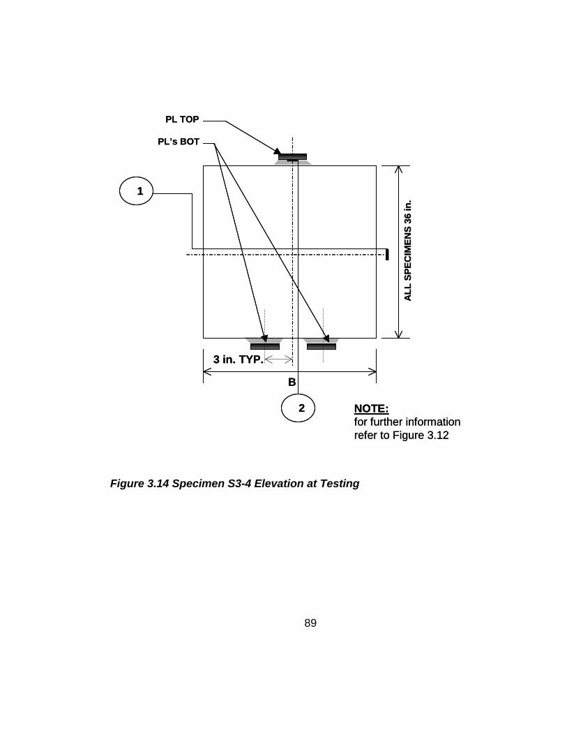
B
ALL
SPE
CIM
ENS
36 in
.
PL TOP
PL’s BOT
2
1
3 in. TYP.
NOTE:for further informationrefer to Figure 3.12
B
ALL
SPE
CIM
ENS
36 in
.
PL TOP
PL’s BOT
2
1
3 in. TYP.
NOTE:for further informationrefer to Figure 3.12
Figure 3.14 Specimen S3-4 Elevation at Testing
89
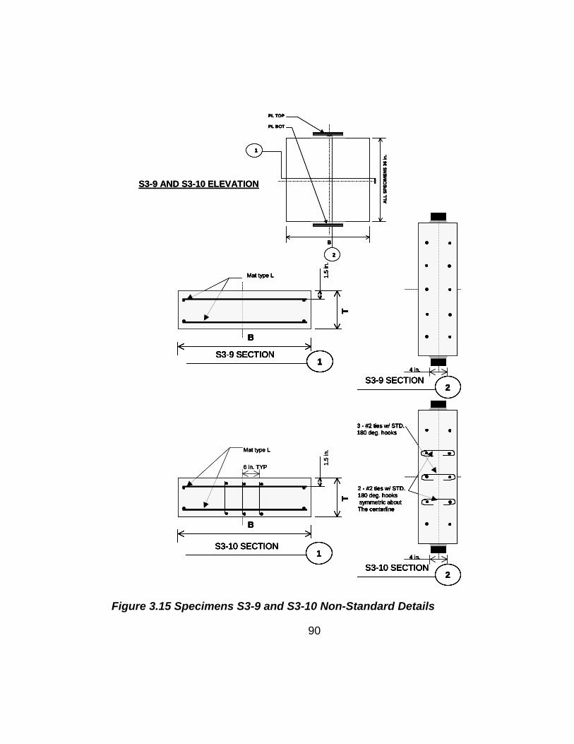
2 - #2 ties w/ STD.180 deg. hookssymmetric about
The centerline
3 - #2 ties w/ STD.180 deg. hooks
4 in.
T
1.5
in.
B
1S3-10 SECTION
6 in. TYP
Mat type L
2S3-10 SECTION
2 - #2 ties w/ STD.180 deg. hookssymmetric about
The centerline
3 - #2 ties w/ STD.180 deg. hooks
4 in.
2 - #2 ties w/ STD.180 deg. hookssymmetric about
The centerline
3 - #2 ties w/ STD.180 deg. hooks
4 in.
T
1.5
in.
B
1S3-10 SECTION
1S3-10 SECTION
6 in. TYP
Mat type L
2S3-10 SECTION
2S3-10 SECTION
4 in.
T
1.5
in.
B
1S3-9 SECTION
Mat type L
2S3-9 SECTION
4 in.
T
1.5
in.
B
1S3-9 SECTION
Mat type L
4 in.
T
1.5
in.
B
1S3-9 SECTION
1S3-9 SECTION
Mat type L
2S3-9 SECTION
2S3-9 SECTION
B
ALL
SPE
CIM
ENS
36 in
.
PL TOP
PL BOT
2
1
B
ALL
SPE
CIM
ENS
36 in
.
PL TOP
PL BOT
2
1
S3-9 AND S3-10 ELEVATION
2 - #2 ties w/ STD.180 deg. hookssymmetric about
The centerline
3 - #2 ties w/ STD.180 deg. hooks
4 in.
T
1.5
in.
B
1S3-10 SECTION
6 in. TYP
Mat type L
2S3-10 SECTION
2 - #2 ties w/ STD.180 deg. hookssymmetric about
The centerline
3 - #2 ties w/ STD.180 deg. hooks
4 in.
2 - #2 ties w/ STD.180 deg. hookssymmetric about
The centerline
3 - #2 ties w/ STD.180 deg. hooks
4 in.
T
1.5
in.
B
1S3-10 SECTION
1S3-10 SECTION
6 in. TYP
Mat type L
2S3-10 SECTION
2S3-10 SECTION
4 in.
T
1.5
in.
B
1S3-9 SECTION
Mat type L
2S3-9 SECTION
4 in.
T
1.5
in.
B
1S3-9 SECTION
Mat type L
4 in.
T
1.5
in.
B
1S3-9 SECTION
1S3-9 SECTION
Mat type L
2S3-9 SECTION
2S3-9 SECTION
B
ALL
SPE
CIM
ENS
36 in
.
PL TOP
PL BOT
2
1
B
ALL
SPE
CIM
ENS
36 in
.
PL TOP
PL BOT
2
1
S3-9 AND S3-10 ELEVATION
Figure 3.15 Specimens S3-9 and S3-10 Non-Standard Details
90

91
4.0 PRESENTATION OF THE TEST RESULTS
4.1 INTRODUCTION
The experimental program described in Chapter 3 is congruent with
similar experimental investigations by many researchers ([11], [13], [21],
[34], [39], [44]) in which specimens were loaded on a surface smaller than
that of the supporting surface of the specimen. In these tests,
compressive stresses spread away from their local introduction to a
uniform stress distribution across the section. Most of these experimental
investigations, with the exception of Sanders [44], concentrated on finding
the ultimate bearing capacity of these specimens by using fracture
mechanics or empirical relationships. Sanders [44] showed that the
stress fields created from the local introduction of a bearing stress may
also be modeled with the strut-and-tie method as bottle-shaped struts.
This type of analysis provided a conservative estimate of the bearing
capacity of the specimen provided that equilibrium and the chosen yield
criteria were satisfied within the model.
The purpose of the experimental investigation reported herein was
to build on the strut-and-tie method of modeling the behavior of specimens
of this type which originated with the work done on NCHRP 10-29 [17],
[39], [44], [51], which were described in Chapter 2.
The remaining experimental investigations that did not model the
behavior of this type of specimens with the strut-and-tie method still
provide some insight into the behavior of bottle-shaped struts and
therefore will be mentioned briefly in the following paragraphs to provide
92
the reader with some basic background information on methods of
previous analyses.
Experimental investigations that resulted in empirical relationships
to describe the behavior of bottle-shaped struts include work done by
Adebar and Zhou [11] in which specimens were tested in a manner similar
to that of a double-punch-tested specimen as shown in Figure 4.1 A. The
specimens were instrumented to capture the cracking load while the ratios
of D/d and H/d were varied. The cracking load is a direct measure of the
tensile strength of concrete in the double-punch configuration. In the
Adebar and Zhou tests the cracking load was a function of both these
ratios. An empirical relationship was produced that limited the
compressive stress to that of the cracking stress for unreinforced
specimens with the assumption that stress redistribution would be limited
without reinforcement. Previous to Adebar and Zhou, Marti [27] provided
a relationship based on fracture mechanics that accounted for the size
effect of the specimens in determining a limiting tensile stress for concrete
using double-punch tests which was substantiated by the work of Adebahr
and Zhou.
More investigations that resulted in empirical relationships to
describe the behavior of bottle-shaped struts are those of Niyogi [34], [35],
[36], and Rigden et. al [13], [14]. The specimens fabricated in theses
investigations were lightly instrumented when reinforcement was present,
and only the ultimate load and failure mechanism was recorded when
reinforcement was not present. Niyogi, presented empirical relationships
based on the plate dimensions relative to the dimension of the loaded
93
surface; while, Rigden et.al presented a relationship based on linear
regression of data to account for type and amount of reinforcement for a
given loading condition.
Hawkins [21], [21] described the behavior of bottle shaped-struts
using fracture mechanics, to model the conical failure cones observed
under the bearing plate for various loading configurations.
In all previous investigations, the experimental data collected
consisted of visual observations, ultimate bearing stresses under the
loading plate, and steel strain gauges when reinforcing bars were present
in the specimens. The current experimental investigation described in
Chapter 3 supplied experimental results of 4 types:
visual observations
ultimate stress under the loaded area
reinforcement strains
concrete strains on the surface of the specimens
The results in these four series are presented sequentially in the
following sections.

D
d
H
Ab
A
e
Ab
A
A) Double Punch Test B) Adebar and Zhou [11]
C) Sanders [44], Roberts [39]Rigden et. Al. [13]
D) Hawkins [21], Niyogi [34]
e
e
D
d
H
D
d
H
Ab
A
e
Ab
A
A) Double Punch Test B) Adebar and Zhou [11]
C) Sanders [44], Roberts [39]Rigden et. Al. [13]
D) Hawkins [21], Niyogi [34]
e
e
Figure 4.1 Specimens Used in Investigating Bottle-Shaped-Struts
94
95
4.2 VISUAL OBSERVATIONS
The failure mechanism initiated in the same manner for all
specimens in that a hairline crack formed at the specimen centerline
parallel to the loading axis as shown in Figure 3.4 and propagated toward
the bearing plate in either direction. The crack did not extend into the
nodal zone, defined as an isosceles triangle with a height equal to half the
bearing plate width, until the specimen was near failure. The next stage of
the failure mechanism followed a trend as the percentage of reinforcement
transverse to this crack increased in the specimens.
At ultimate failure, mechanisms ranged from a tensile failure
(Figure 4.2) resulting in the failure of a plane bi-axially stressed tending to
the crushing of the concrete at or around the nodal area (Figure 4.3) as
the relative percentage of reinforcement increased. In every specimen
tested concrete located directly under the bearing plate developed a
wedge in the basic proportions of an isosceles triangle. In specimens with
higher quantities of transverse reinforcement wedge concrete forming the
node became smaller and more pronounced. Figure 4.2 displays the
ultimate failure mechanisms for some “lightly” reinforced specimens while
figure 4.3 displays the ultimate failure mechanisms for a number of
specimens with higher percentages of transverse reinforcement. Figure
4.2 also shows the wedge of nodal concrete for specimen S3-10 which,
with specimen S3-9, are the only specimens tested in which the bearing
plate dimension was less than that of the thickness of the specimen

96
resulting in the three-dimensional confinement of the node by the
surrounding concrete. Specimens S3-9 and S3-10 exhibited the tensile
failure mechanism. In one case, specimen S2-8 (Figure 4-2) the failure
plane is slightly inclined at the nodal region, as an extension of the tensile
crack initiating at the specimen centerline. S2-8 contained #2 bars at 8
inches on center placed at 45 degrees to the load axis in two layers
(Figure 3.13 F).
Figure 4.3 displays specimens with reinforcement percentages that
force the failure mechanism from the tensile failures away from the node
to crushing of the concrete at the node face. In these specimens the
nodal area of concrete is apparent when extraneous crushed concrete is
removed.
Figure 4.4 displays a basic comparison of two specimens with
same reinforcement regime. The reinforcement for specimen S2-8 is as
described above. S2-6 contained #3 bars at 6 inches on center oriented
at 45 degrees relative to the load axis (Figure 3.13 E), placed in two
orthogonal layers. The reinforcement percentage given in this figure is the
component of total amount of reinforcement on plane parallel with the
transverse axis. The νe value shown in this figure is the ultimate bearing
stress normalized to the concrete strength. Comparing the failure
mechanisms in this manner the specimens can be classified as “confined”
since they exhibited the crushing failure and pronounced nodal wedge or
“unconfined” which exhibit the tensile failure mechanism.

S1-2
S1-4
S2-8
NODE INVERTED
S3-10
NODE
S1-2
S1-4
S2-8
NODE INVERTED
S3-10
NODE
Figure 4.2 Tensile Failure Mechanism
97
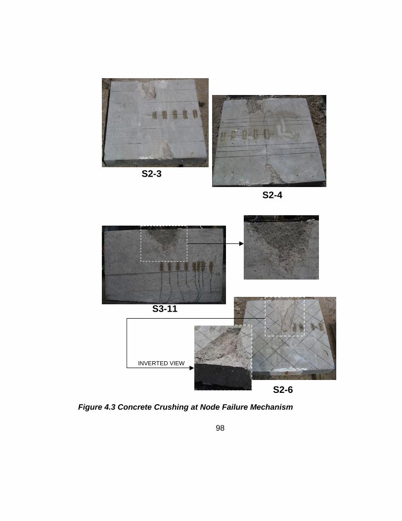
INVERTED VIEW
S2-3
S2-4
S3-11
S2-6 Figure 4.3 Concrete Crushing at Node Failure Mechanism
98
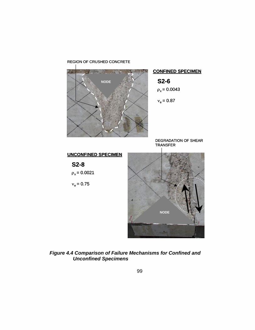
REGION OF CRUSHED CONCRETE
DEGRADATION OF SHEAR TRANSFER
NODE
NODE
ρx = 0.0043
S2-6
CONFINED SPECIMEN
νe = 0.87
ρx = 0.0021
S2-8
UNCONFINED SPECIMEN
νe = 0.75
REGION OF CRUSHED CONCRETE
DEGRADATION OF SHEAR TRANSFER
NODE
NODE
ρx = 0.0043
S2-6
CONFINED SPECIMEN
νe = 0.87
ρx = 0.0021
S2-8
UNCONFINED SPECIMEN
νe = 0.75
Figure 4.4 Comparison of Failure Mechanisms for Confined and Unconfined Specimens
99

The degradation of shear transfer reported by Wollman [51] is
shown in specimen S2-8 in Figure 4.4. Figure 4.5 presents a similar
degradation as the point where the internal angle of friction of the concrete
is less than that of the coefficient of static friction between to rough
concrete surface areas. The concrete in confined specimens crushes
before significant shear degradation occurs.
Δ
A) Confined Specimens
concrete crushing atnode-strut interface
B) Unconfined Specimens
degradation of sheartransfer before crushing
tanφ<μ , σ>σcrush tanφ>μ , σ<σcrush
φ
tensile forceprovided by reinforcing bars
tensile forceprovided by reinforcing bars
Δ
A) Confined Specimens
concrete crushing atnode-strut interface
B) Unconfined Specimens
degradation of sheartransfer before crushing
tanφ<μ , σ>σcrush tanφ>μ , σ<σcrush
φφ
tensile forceprovided by reinforcing bars
tensile forceprovided by reinforcing bars
Figure 4.5 Degradation of Shear-Transfer for Unconfined Specimens
100
101
In the case of confined specimens a secondary failure mechanism
was observed at or immediately after the crushed concrete at the node as
shown in Figure 4.6. This mechanism can be described as splitting tensile
failure initiating at the bearing plate and propagating down the loaded
surface of the specimen. In some cases the tensile crack propagated
down the outer edge of the specimen parallel to the load axis. It is likely
that this mechanism began to form as the node was forced toward the
transverse axis generating a cleaving action in the specimen. For
specimen S2-10, the most heavily reinforced specimen, this failure
occurred simultaneously with concrete crushing around the node resulting
in an extremely explosive and brittle failure. It is also interesting to note
that crack on the loaded surface only appeared to the side of the node in
which concrete has crushed, which is an indication that these failure
mechanism are linked.
4.2.1 Summary of the Results Obtained from Visual Observations
It is clear from the observation of the failure mechanism of these
specimens that, as the percentage of transverse reinforcement increased,
the failure mechanism changed from a tensile failure on planes away from
the nodal area to compressive failures at or near the nodal face. A
secondary tensile failure along the loaded surface associated with the
compressive failure of “heavily” reinforced specimens is also apparent.
The observed failure mechanism can be used to classify the specimen as
either “confined” exhibiting the crushing failure or “unconfined” exhibiting
the tensile failure.

S3-3
S2-9
S2-9 maximum transverse reinforcementwithin experimental investigation
S2-4 crack on bearing surface to the same side as crushed concrete
Crushed concrete
crack propagates from the bearing plate in everyspecimen that it occurred
S3-3
S2-9
S2-9 maximum transverse reinforcementwithin experimental investigation
S2-4 crack on bearing surface to the same side as crushed concrete
Crushed concrete
crack propagates from the bearing plate in everyspecimen that it occurred
Figure 4.6 Secondary Failure Mechanism Associated with “Heavily”
Reinforced Specimens
102
103
4.3 ULTIMATE STRESS UNDER LOADED AREA
After cracking and ultimate stresses under the bearing plate area
were normalized with respect to f`c (νe - ultimate efficiency factor, νc -
cracking efficiency factor) to allow comparisons, a distinct categorization
was apparent. The ultimate load carried by the specimens was a function
of reinforcement provided, the ratio of cross-sectional area to that of the
bearing plate area (A=bt/Ab), as well as, the ratio of the height of the
specimen to the thickness of the specimen.
Furthermore, the three specimens in series 1 (S1-3, S1-4, S1-5)
which had nodal confinement in the form of closed ties had high bearing
capacities relative to those which contained similar reinforcement and A/Ab
ratios. The ultimate capacities of specimens S1-3, S1-4, and S1-5
however, were less than those specimens with higher A/Ab rations with no
confinement of the node.
Specimens S3-9, and 3-10, which also had the largest bt/Ab ratios
and similar reinforcement ratios as specimens S2-3, S2-4, S2-7, S3-4 and
S3-7, exhibited the largest capacity. The ultimate bearing capacities are
shown in increasing order in Figure 4.7, and grouped according to their
geometric ratios (A/Ab, h/2b).
The term νe - νc or the normalized ultimate stress less the
normalized cracking stress is an indicator of the level of redistribution in
the specimens. This term is plotted in Figure 4.8, and it is apparent that
the level of redistribution is proportional to A/Ab ratio. This behavior is
similar to that observed by Adebar and Zhou [11]. The first group of

specimens is plotted in Figure 4.9, in which there is the most drastic
variation of transverse reinforcement; it is apparent that the amount of
stress redistribution is directly proportional to the amount of reinforcement
provided.
A/Ab = 3h/2b = 3
A/Ab = 3h/2b = 4.5
A/Ab = 6h/2b = 3
A/Ab = 7.5h/2b = 4.5
A/Ab = 5h/2b = 3
A/Ab = 3.75h/2b = 3
0
0.1
0.2
0.3
0.4
0.5
0.6
0.7
0.8
0.9
1
1.1
1.2
1.3
1.4
1.5
S3-
1S
3-2
S2-
8S
3-12
S3-
6S
2-2
S3-
5S
2-6
S2-
7S
3-11
S2-
9S
2-4
S3-
3S
2-10
S2-
3
S1-
2S
1-4
S1-
5S
1-3
S1-
1
S3-
8S
3-7
S3-
4
S3-
9S
3-10
h/2
A
Ab
b
νe
0
0.1
0.2
0.3
0.4
0.5
0.6
0.7
0.8
0.9
1
1.1
1.2
1.3
1.4
1.5
S3-
1S
3-2
S2-
8S
3-12
S3-
6S
2-2
S3-
5S
2-6
S2-
7S
3-11
S2-
9S
2-4
S3-
3S
2-10
S2-
3
S1-
2S
1-4
S1-
5S
1-3
S1-
1
S3-
8S
3-7
S3-
4
S3-
9S
3-10
h/2
A
Ab
bh/2
A
Ab
b
νe
Figure 4.7 Ultimate Capacities
104
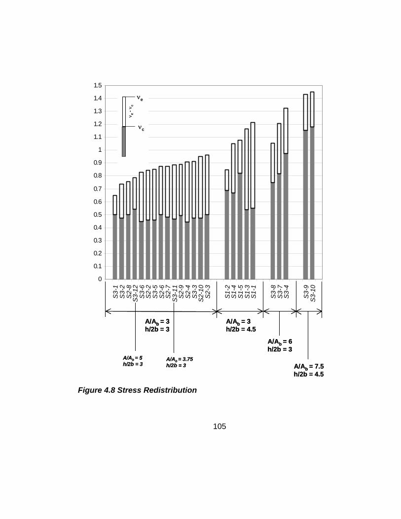
0
0.1
0.2
0.3
0.4
0.5
0.6
0.7
0.8
0.9
1
1.1
1.2
1.3
1.4
1.5
S3-
1S
3-2
S2-
8S
3-12
S3-
6S
2-2
S3-
5S
2-6
S2-
7S
3-11
S2-
9S
2-4
S3-
3S
2-10
S2-
3
S1-
2S
1-4
S1-
5S
1-3
S1-
1
S3-
8S
3-7
S3-
4
S3-
9S
3-10
A/Ab = 3h/2b = 3
A/Ab = 3h/2b = 4.5
A/Ab = 6h/2b = 3
A/Ab = 7.5h/2b = 4.5
A/Ab = 5h/2b = 3
A/Ab = 3.75h/2b = 3
νe
ν e -
ν c
νc
νe
ν e -
ν c
νc
Figure 4.8 Stress Redistribution
105
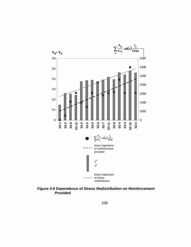
0
0.1
0.2
0.3
0.4
0.5
0.6S3
-1
S3-2
S2-8
S3-1
2
S3-6
S2-2
S3-5
S2-6
S2-7
S3-1
1
S2-9
S2-4
S3-3
S2-1
0
S2-3
0
0.001
0.002
0.003
0.004
0.005
0.006
0.007
n
Asi
b si⋅.⋅ sin γi( )
fy
63 ksi⋅⋅∑
νe- νc
ν e -
ν c
n
Asi
b si⋅.⋅ sin γi( )
fy
63 ksi⋅⋅∑
n
Asi
b si⋅.⋅ sin γi( )
fy
63 ksi⋅⋅∑
linear regression of reinforcement provided
linear regression of stress redistribution
0
0.1
0.2
0.3
0.4
0.5
0.6S3
-1
S3-2
S2-8
S3-1
2
S3-6
S2-2
S3-5
S2-6
S2-7
S3-1
1
S2-9
S2-4
S3-3
S2-1
0
S2-3
0
0.001
0.002
0.003
0.004
0.005
0.006
0.007
n
Asi
b si⋅.⋅ sin γi( )
fy
63 ksi⋅⋅∑
n
Asi
b si⋅.⋅ sin γi( )
fy
63 ksi⋅⋅∑
νe- νc
ν e -
ν c
n
Asi
b si⋅.⋅ sin γi( )
fy
63 ksi⋅⋅∑
n
Asi
b si⋅.⋅ sin γi( )
fy
63 ksi⋅⋅∑
linear regression of reinforcement provided
linear regression of stress redistribution
ν e -
ν c
n
Asi
b si⋅.⋅ sin γi( )
fy
63 ksi⋅⋅∑
n
Asi
b si⋅.⋅ sin γi( )
fy
63 ksi⋅⋅∑
linear regression of reinforcement provided
linear regression of stress redistribution
Figure 4.9 Dependence of Stress Redistribution on Reinforcement Provided
106
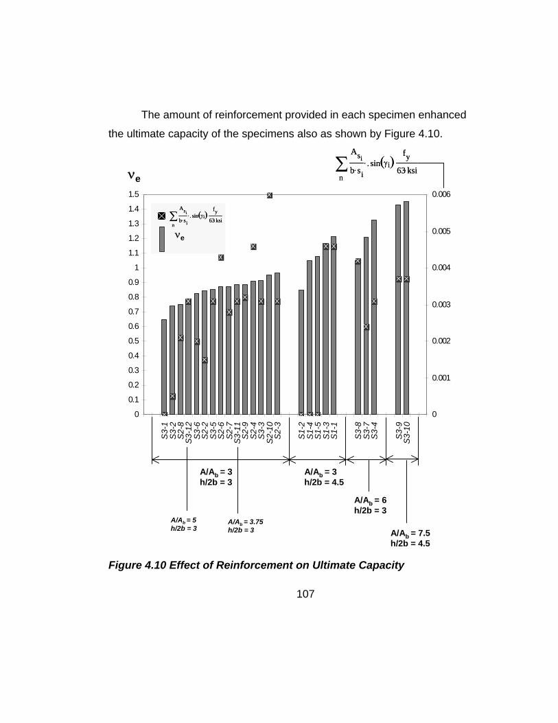
The amount of reinforcement provided in each specimen enhanced
the ultimate capacity of the specimens also as shown by Figure 4.10.
0
0.1
0.2
0.3
0.4
0.5
0.6
0.7
0.8
0.9
1
1.1
1.2
1.3
1.4
1.5
S3-
1S
3-2
S2-
8S
3-12
S3-
6S
2-2
S3-
5S
2-6
S2-
7S
3-11
S2-
9S
2-4
S3-
3S
2-10
S2-
3
S1-
2S
1-4
S1-
5S
1-3
S1-
1
S3-
8S
3-7
S3-
4
S3-
9S
3-10
0
0.001
0.002
0.003
0.004
0.005
0.006
n
Asi
b si⋅.⋅ sin γi( )
fy
63 ksi⋅⋅∑
n
Asi
b si⋅.⋅ sin γi( )
fy
63 ksi⋅⋅∑
νe
A/Ab = 3h/2b = 3
A/Ab = 3h/2b = 4.5
A/Ab = 6h/2b = 3
A/Ab = 7.5h/2b = 4.5
A/Ab = 5h/2b = 3
A/Ab = 3.75h/2b = 3
n
Asi
b si⋅.⋅ sin γi( )
fy
63 ksi⋅⋅∑
n
Asi
b si⋅.⋅ sin γi( )
fy
63 ksi⋅⋅∑
νe
n
Asi
b si⋅.⋅ sin γi( )
fy
63 ksi⋅⋅∑
n
Asi
b si⋅.⋅ sin γi( )
fy
63 ksi⋅⋅∑
νe
Figure 4.10 Effect of Reinforcement on Ultimate Capacity
107
108
It is apparent from Figure 4.10 that there is an upper limit on the increase
in the ultimate capacity attributable to the reinforcement provided.
Specimen S2-10 had a relative reinforcement ratio twice that of specimen
S2-3 yet the capacities were similar. For A/Ab ratios equal to 6, it appears
that the reinforcement provided had little or no effect on the capacity.
Specimen S3-8 had the greatest amount of reinforcement yet the lowest
capacity within the group. This specimen was reinforced with #3 bars at 6
inches on center placed in an orthogonal mat that was rotated at an angle
of 30 degrees relative to the load axis resulting in half the reinforcement at
an angle of 30 degrees relative to the load axis and half the reinforcement
at an angle of 60 degrees relative to the load axis (Figure 3.13 K). The
configuration of the reinforcement was not efficient in confining the
specimen and therefore the ultimate capacity is lower than those
specimens in the group with less reinforcement placed perpendicular to
the load axis of the specimen. The reinforcement provided in specimen
S3-9 was placed in two mats near the outer surfaces of the specimen
(Figure 3.15). The reinforcement provided in S3-10 was identical to S3-9
with an additional 35 % of transvere reinforcement placed as ties between
the two layers of steel placed near the form and finished faces (Figure
3.15). Both configurations of reinforcement were inefficient in further
enhancing the ultimate capacity of the specimen and are consistent with
the findings of Rigden et al [13].
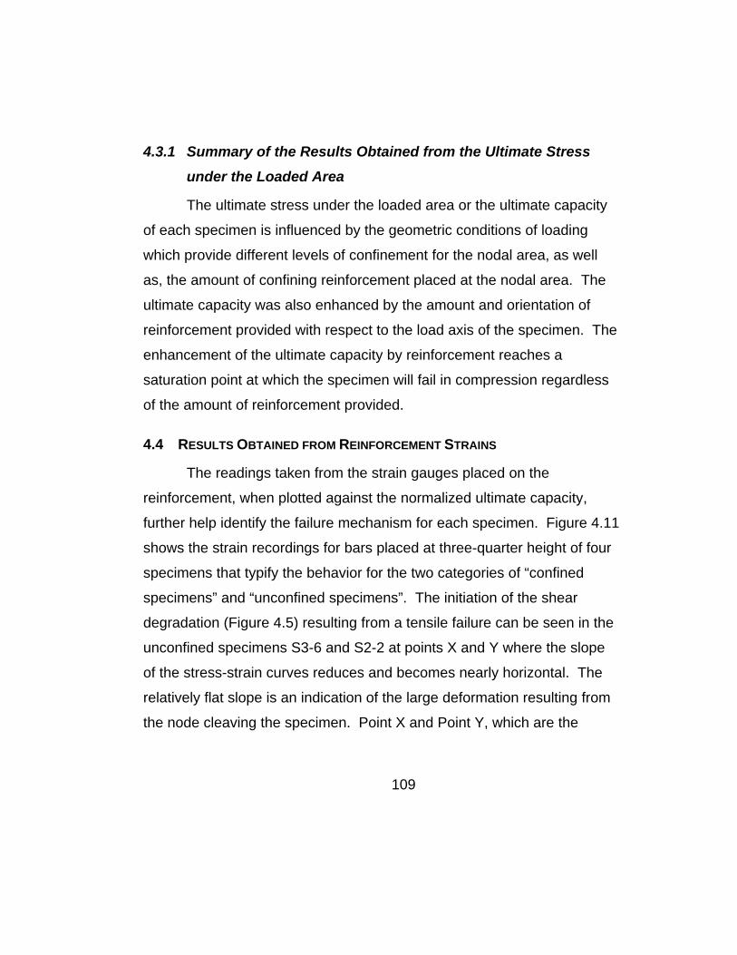
109
4.3.1 Summary of the Results Obtained from the Ultimate Stress
under the Loaded Area
The ultimate stress under the loaded area or the ultimate capacity
of each specimen is influenced by the geometric conditions of loading
which provide different levels of confinement for the nodal area, as well
as, the amount of confining reinforcement placed at the nodal area. The
ultimate capacity was also enhanced by the amount and orientation of
reinforcement provided with respect to the load axis of the specimen. The
enhancement of the ultimate capacity by reinforcement reaches a
saturation point at which the specimen will fail in compression regardless
of the amount of reinforcement provided.
4.4 RESULTS OBTAINED FROM REINFORCEMENT STRAINS
The readings taken from the strain gauges placed on the
reinforcement, when plotted against the normalized ultimate capacity,
further help identify the failure mechanism for each specimen. Figure 4.11
shows the strain recordings for bars placed at three-quarter height of four
specimens that typify the behavior for the two categories of “confined
specimens” and “unconfined specimens”. The initiation of the shear
degradation (Figure 4.5) resulting from a tensile failure can be seen in the
unconfined specimens S3-6 and S2-2 at points X and Y where the slope
of the stress-strain curves reduces and becomes nearly horizontal. The
relatively flat slope is an indication of the large deformation resulting from
the node cleaving the specimen. Point X and Point Y, which are the
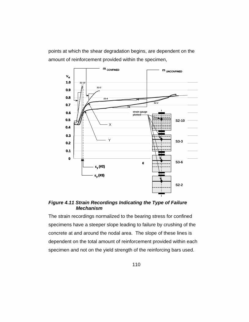
points at which the shear degradation begins, are dependent on the
amount of reinforcement provided within the specimen,
X
Y
1.0
0.9
0.8
0.7
0.6
0.5
0.4
0.3
0.2
0.1
0
m CONFINED m UNCONFINED
S3-3
S2-10
S3-6
S2-2
εy (#3)
εy (#2)ε
νe
S2-10
S3-3
S3-6
S2-2
strain gaugeplotted
X
Y
1.0
0.9
0.8
0.7
0.6
0.5
0.4
0.3
0.2
0.1
0
m CONFINED m UNCONFINED
S3-3
S2-10
S3-6
S2-2
εy (#3)
εy (#2)ε
νe
S2-10
S3-3
S3-6
S2-2
strain gaugeplotted
X
Y
1.0
0.9
0.8
0.7
0.6
0.5
0.4
0.3
0.2
0.1
0
m CONFINED m UNCONFINED
S3-3
S2-10
S3-6
S2-2
εy (#3)
εy (#2)ε
νe
S2-10
S3-3
S3-6
S2-2
strain gaugeplotted
S2-10
S3-3
S3-6
S2-2
S2-10
S3-3
S3-6
S2-2
strain gaugeplotted
Figure 4.11 Strain Recordings Indicating the Type of Failure
Mechanism The strain recordings normalized to the bearing stress for confined
specimens have a steeper slope leading to failure by crushing of the
concrete at and around the nodal area. The slope of these lines is
dependent on the total amount of reinforcement provided within each
specimen and not on the yield strength of the reinforcing bars used.
110
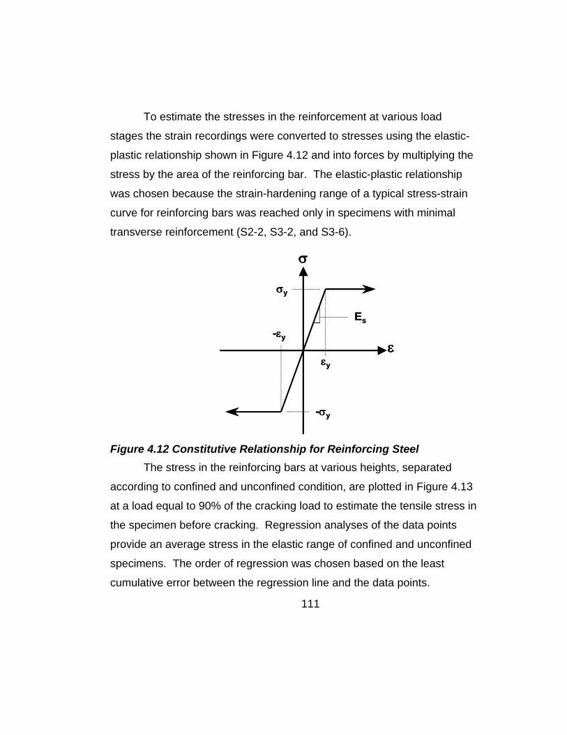
To estimate the stresses in the reinforcement at various load
stages the strain recordings were converted to stresses using the elastic-
plastic relationship shown in Figure 4.12 and into forces by multiplying the
stress by the area of the reinforcing bar. The elastic-plastic relationship
was chosen because the strain-hardening range of a typical stress-strain
curve for reinforcing bars was reached only in specimens with minimal
transverse reinforcement (S2-2, S3-2, and S3-6).
ε
σ
εy
σy
-σy
-εy
Es
ε
σ
εy
σy
-σy
-εy
Es
Figure 4.12 Constitutive Relationship for Reinforcing Steel
The stress in the reinforcing bars at various heights, separated
according to confined and unconfined condition, are plotted in Figure 4.13
at a load equal to 90% of the cracking load to estimate the tensile stress in
the specimen before cracking. Regression analyses of the data points
provide an average stress in the elastic range of confined and unconfined
specimens. The order of regression was chosen based on the least
cumulative error between the regression line and the data points.
111
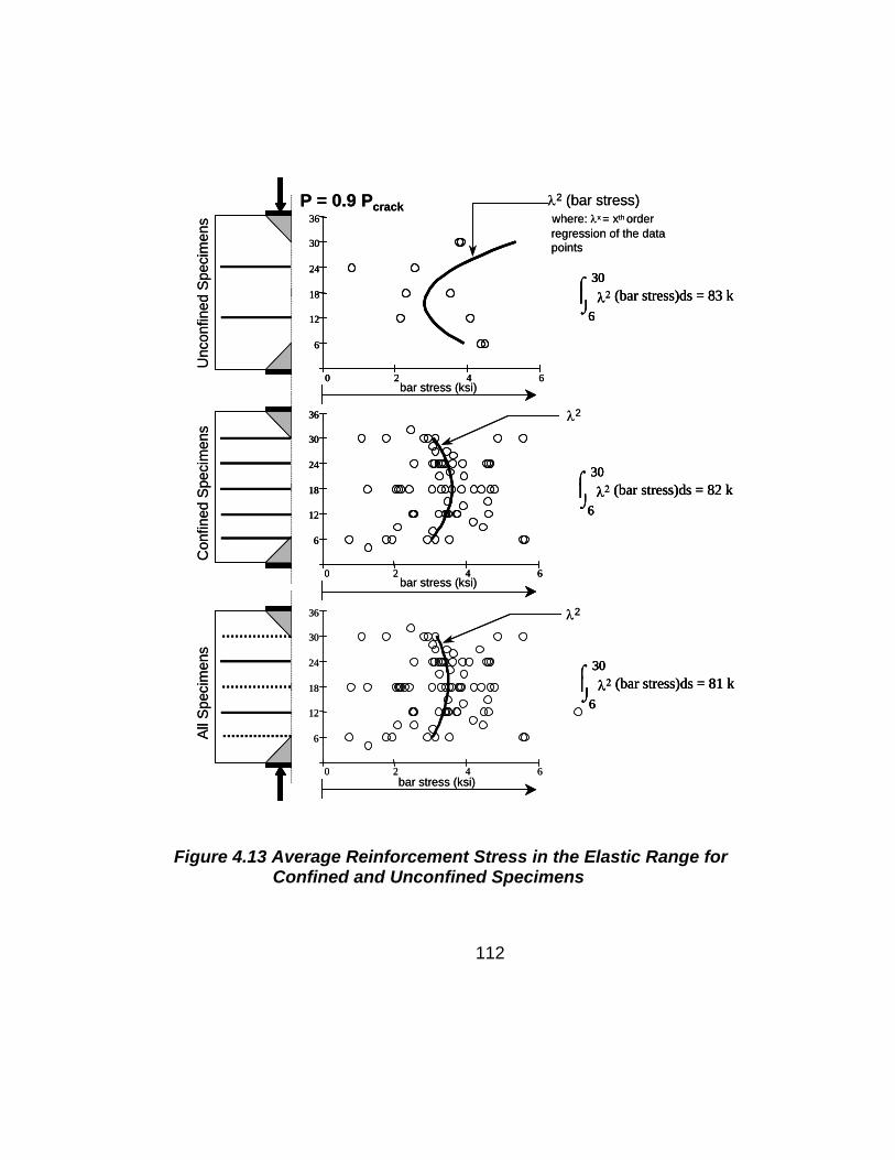
Unc
onfin
ed S
peci
men
sC
onfin
ed S
peci
men
sAl
l Spe
cim
ens
P = 0.9 Pcrack
0 2 4 6
6
12
18
24
30
36
λ2 (bar stress)where: λx = xth order regression of the datapoints
bar stress (ksi)
bar stress (ksi)
bar stress (ksi)
λ2
λ2
0 2 4 6
6
12
18
24
30
36
0 2 4 6
6
12
18
24
30
36
λ2 (bar stress)ds = 81 k 6
30⌠⎮⌡
λ2 (bar stress)ds = 82 k 6
30⌠⎮⌡
λ2 (bar stress)ds = 83 k 6
30⌠⎮⌡
Unc
onfin
ed S
peci
men
sC
onfin
ed S
peci
men
sAl
l Spe
cim
ens
P = 0.9 Pcrack
0 2 4 6
6
12
18
24
30
36
0 2 4 6
6
12
18
24
30
36
λ2 (bar stress)where: λx = xth order regression of the datapoints
bar stress (ksi)
bar stress (ksi)
bar stress (ksi)
λ2
λ2
0 2 4 6
6
12
18
24
30
36
0 2 4 6
6
12
18
24
30
36
0 2 4 6
6
12
18
24
30
36
λ2 (bar stress)ds = 81 k 6
30⌠⎮⌡
λ2 (bar stress)ds = 81 k 6
30⌠⎮⌡6
30⌠⎮⌡
λ2 (bar stress)ds = 82 k 6
30⌠⎮⌡
λ2 (bar stress)ds = 82 k 6
30⌠⎮⌡6
30⌠⎮⌡
λ2 (bar stress)ds = 83 k 6
30⌠⎮⌡
λ2 (bar stress)ds = 83 k 6
30⌠⎮⌡6
30⌠⎮⌡
Figure 4.13 Average Reinforcement Stress in the Elastic Range for Confined and Unconfined Specimens
112
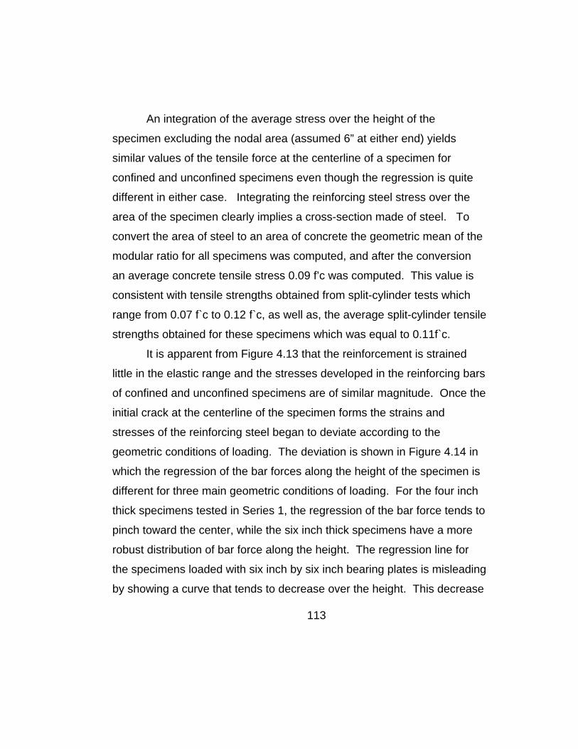
113
An integration of the average stress over the height of the
specimen excluding the nodal area (assumed 6” at either end) yields
similar values of the tensile force at the centerline of a specimen for
confined and unconfined specimens even though the regression is quite
different in either case. Integrating the reinforcing steel stress over the
area of the specimen clearly implies a cross-section made of steel. To
convert the area of steel to an area of concrete the geometric mean of the
modular ratio for all specimens was computed, and after the conversion
an average concrete tensile stress 0.09 f’c was computed. This value is
consistent with tensile strengths obtained from split-cylinder tests which
range from 0.07 f`c to 0.12 f`c, as well as, the average split-cylinder tensile
strengths obtained for these specimens which was equal to 0.11f`c.
It is apparent from Figure 4.13 that the reinforcement is strained
little in the elastic range and the stresses developed in the reinforcing bars
of confined and unconfined specimens are of similar magnitude. Once the
initial crack at the centerline of the specimen forms the strains and
stresses of the reinforcing steel began to deviate according to the
geometric conditions of loading. The deviation is shown in Figure 4.14 in
which the regression of the bar forces along the height of the specimen is
different for three main geometric conditions of loading. For the four inch
thick specimens tested in Series 1, the regression of the bar force tends to
pinch toward the center, while the six inch thick specimens have a more
robust distribution of bar force along the height. The regression line for
the specimens loaded with six inch by six inch bearing plates is misleading
by showing a curve that tends to decrease over the height. This decrease
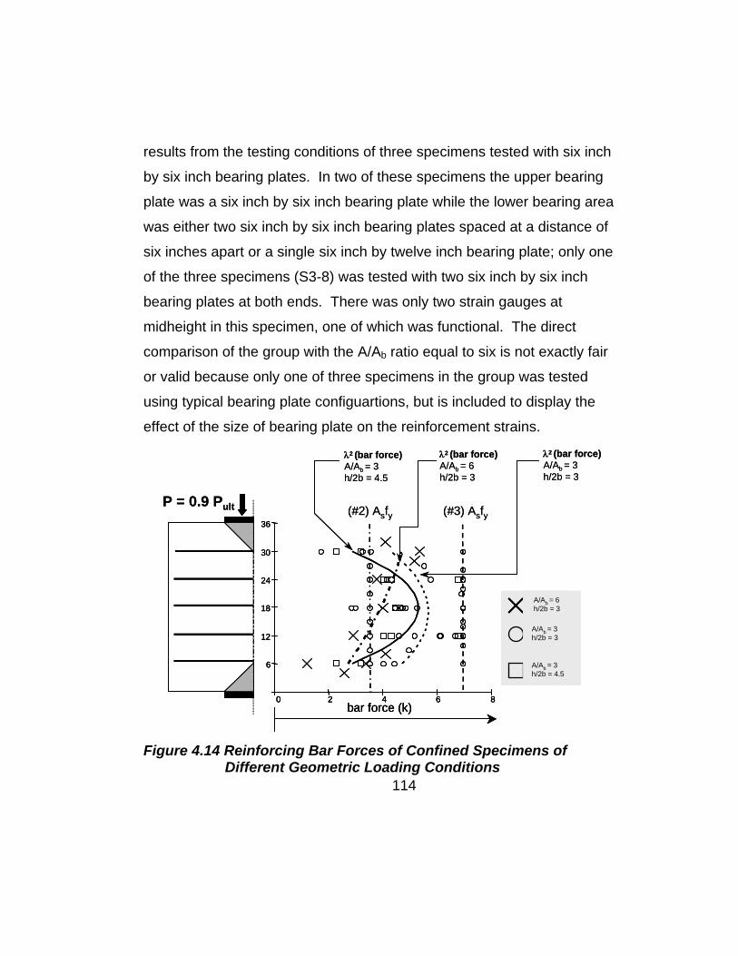
results from the testing conditions of three specimens tested with six inch
by six inch bearing plates. In two of these specimens the upper bearing
plate was a six inch by six inch bearing plate while the lower bearing area
was either two six inch by six inch bearing plates spaced at a distance of
six inches apart or a single six inch by twelve inch bearing plate; only one
of the three specimens (S3-8) was tested with two six inch by six inch
bearing plates at both ends. There was only two strain gauges at
midheight in this specimen, one of which was functional. The direct
comparison of the group with the A/Ab ratio equal to six is not exactly fair
or valid because only one of three specimens in the group was tested
using typical bearing plate configuartions, but is included to display the
effect of the size of bearing plate on the reinforcement strains.
(#2) Asfy (#3) AsfyP = 0.9 Pult
λ2 (bar force)A/Ab = 3h/2b = 4.5
λ2 (bar force)A/Ab = 6h/2b = 3
λ2 (bar force)A/Ab = 3h/2b = 3
bar force (k)0 2 4 6 8
6
12
18
24
30
36
A/Ab = 3h/2b = 4.5
A/Ab = 6h/2b = 3
A/Ab = 3h/2b = 3
(#2) Asfy (#3) AsfyP = 0.9 Pult
λ2 (bar force)A/Ab = 3h/2b = 4.5
λ2 (bar force)A/Ab = 6h/2b = 3
λ2 (bar force)A/Ab = 3h/2b = 3
bar force (k)bar force (k)0 2 4 6 8
6
12
18
24
30
36
0 2 4 6 8
6
12
18
24
30
36
A/Ab = 3h/2b = 4.5
A/Ab = 6h/2b = 3
A/Ab = 3h/2b = 3
A/Ab = 3h/2b = 4.5
A/Ab = 6h/2b = 3
A/Ab = 3h/2b = 3
114
Figure 4.14 Reinforcing Bar Forces of Confined Specimens of Different Geometric Loading Conditions

A direct comparison of the regression of bar forces along the height
of the specimen of confined and unconfined specimens was made, and is
shown in Figure 4.15. From this figure, the average bar force is higher at
the loaded surfaces of the specimen for unconfined behavior opposed to
confined behavior which shows a robust distribution of bar force along the
height of the specimen with maximum force was reached at mid-height.
P = 0.9 Pult (#3) Asfy(#2) Asfy
λ2 (bar force)all confined specimensexcept S3-9 and S3-10
bar force (k)
λ2 (bar force)all unconfined specimens
0 2 4 6 8
6
12
18
24
30
36
P = 0.9 PultP = 0.9 Pult (#3) Asfy(#2) Asfy
λ2 (bar force)all confined specimensexcept S3-9 and S3-10
bar force (k)bar force (k)
λ2 (bar force)all unconfined specimens
0 2 4 6 8
6
12
18
24
30
36
0 2 4 6 8
6
12
18
24
30
36
Figure 4.15 Reinforcing Bar Forces of Confined and Unconfined
Specimens For the two three-dimensional specimens tested (S3-9, S3-10) the
bar stresses parallel to failure plane are stressed to 60-70% of their yield
stress values. In Specimen S3-10, reinforcement was placed
perpendicular to the failure plane, and Figure 4.16 shows that the stresses
in these bars were around 3% of the forces in the bars parallel to the
failure plane. From Figure 4.16, it would appear that the reinforcement
115

which directly crossed the failure plane was highly inefficient in
redistributing the stresses after cracking, more so than reinforcement
placed at the outer edges parallel to the failure plane. This could also be
an indication that reinforcement of this type does little to enhance the
capacity of three-dimensional specimens. A more suitable type of
reinforcing arrangement would be closed ties around the perimeter of the
specimens as suggested by Rigden et al [11].
0 20 40 60
6
12
18
24
30
36
_
_
P = 0.9 Pult
S3-9
S3-1
0S3
-10
tran
sver
se to
sp
littin
g cr
ack
failure plane for specimens S3-9 and S3-10
0 20 40 60
6
12
18
24
30
36
_
0 20 40 60
6
12
18
24
30
36
_
Bar Stress (ksi)
Bar Stress (ksi)
Bar Stress (ksi)
0 20 40 60
6
12
18
24
30
36
_
_
P = 0.9 Pult
S3-9
S3-1
0S3
-10
tran
sver
se to
sp
littin
g cr
ack
failure plane for specimens S3-9 and S3-10
0 20 40 60
6
12
18
24
30
36
_
0 20 40 60
6
12
18
24
30
36
_
Bar Stress (ksi)
Bar Stress (ksi)
Bar Stress (ksi)
Figure 4.16 Reinforcing Bar Forces for Three-Dimensional
Specimens
116
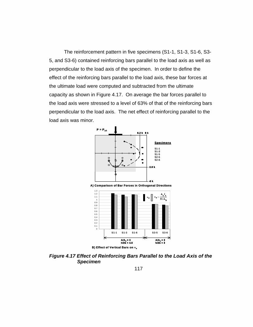
The reinforcement pattern in five specimens (S1-1, S1-3, S1-6, S3-
5, and S3-6) contained reinforcing bars parallel to the load axis as well as
perpendicular to the load axis of the specimen. In order to define the
effect of the reinforcing bars parallel to the load axis, these bar forces at
the ultimate load were computed and subtracted from the ultimate
capacity as shown in Figure 4.17. On average the bar forces parallel to
the load axis were stressed to a level of 63% of that of the reinforcing bars
perpendicular to the load axis. The net effect of reinforcing parallel to the
load axis was minor.
P = Pult
-8 k
8 k6.2 k
-3.9 k
Specimens
S1-1S1-3S1-5S2-5S2-6
00.10.20.30.40.50.60.70.80.9
11.11.21.3
S1-1 S1-3 S1-6 S3-5 S3-6
A/Ab = 3h/2b = 3
A/Ab = 3h/2b = 4.5
ν eAs fs
f'c A b⋅−ν e
A) Comparison of Bar Forces in Orthogonal Directions
B) Effect of Vertical Bars on νe
P = Pult
-8 k
8 k6.2 k
-3.9 k
P = Pult
-8 k
8 k6.2 k
-3.9 k
Specimens
S1-1S1-3S1-5S2-5S2-6
00.10.20.30.40.50.60.70.80.9
11.11.21.3
S1-1 S1-3 S1-6 S3-5 S3-6
A/Ab = 3h/2b = 3
A/Ab = 3h/2b = 4.5
ν eAs fs
f'c A b⋅−ν e
00.10.20.30.40.50.60.70.80.9
11.11.21.3
S1-1 S1-3 S1-6 S3-5 S3-6
A/Ab = 3h/2b = 3
A/Ab = 3h/2b = 4.5
ν eAs fs
f'c A b⋅−ν e ν e
As fsf'c A b⋅
−ν e ν eAs fs
f'c A b⋅−ν e
As fsf'c A b⋅
−ν eν e
A) Comparison of Bar Forces in Orthogonal Directions
B) Effect of Vertical Bars on νe Figure 4.17 Effect of Reinforcing Bars Parallel to the Load Axis of the
Specimen
117
While keeping the percentage of reinforcement relatively constant
as well as the geometric conditions of loading (A/Ab = constant, h/2b =
constant), the orientation, size, and distribution of the reinforcement varied
in several specimens. The effect of the orientation, size, and distribution
of reinforcement had little effect on the ultimate capacity of the specimens
as shown in Figure 4.18.
0
0.1
0.2
0.3
0.4
0.5
0.6
0.7
0.8
0.9
1
S2-6 S2-9 S2-4 S3-30
0.001
0.002
0.003
0.004
0.005
#3 bars #2 bars #3 bars #3 bars
n
Asi
b si⋅.⋅ sin γi( )
fy
63 ksi⋅⋅∑
νe
n
Asi
b si⋅.⋅ sin γi( )
fy
63 ksi⋅⋅∑
n
Asi
b si⋅.⋅ sin γi( )
fy
63 ksi⋅⋅∑
νe
0
0.1
0.2
0.3
0.4
0.5
0.6
0.7
0.8
0.9
1
S2-6 S2-9 S2-4 S3-30
0.001
0.002
0.003
0.004
0.005
#3 bars #2 bars #3 bars #3 bars
n
Asi
b si⋅.⋅ sin γi( )
fy
63 ksi⋅⋅∑
n
Asi
b si⋅.⋅ sin γi( )
fy
63 ksi⋅⋅∑
νe
n
Asi
b si⋅.⋅ sin γi( )
fy
63 ksi⋅⋅∑
n
Asi
b si⋅.⋅ sin γi( )
fy
63 ksi⋅⋅∑
νe
n
Asi
b si⋅.⋅ sin γi( )
fy
63 ksi⋅⋅∑
n
Asi
b si⋅.⋅ sin γi( )
fy
63 ksi⋅⋅∑
νe
Figure 4.18 Effect of Variations of Reinforcement on the Ultimate
Capacity of the Specimen
118
119
4.4.1 Summary of the Results Obtained from Reinforcement Strains
For planar specimens the amount of reinforcement provided
enhanced the ultimate load carrying capacity of the specimen, with a
stress redistribution occurring past the initial cracking and in some cases
pass the yield point of the reinforcing bars. For confined behavior a
saturation level is apparent by comparing specimens S2-3 and S2-10
which had similar capacities yet specimen S2-10 had twice the percentage
of reinforcement as S2-3. For the same percentage of reinforcing steel
provided, the orientation of reinforcing bars either perpendicular to the
load axis or at angles of 45 degrees produced the same level of
enhancement and a confined failure while reinforcing bars placed at angle
less than 45 degrees relative to the load axis produced an unconfined
failure of specimen S3-8. Furthermore lumped reinforcing and distributed
reinforcing of the same amount produced similar effects either providing a
confined or unconfined failure of the specimen depending on the amount
of reinforcement provided. Reinforcing bars parallel to the load axis of the
specimen provided little enhancement to the ultimate capacity or
influenced the type of failure.
An interesting result obtained from the reinforcing strains is that the
tensile forces in the reinforcing bars of specimens exhibiting the
unconfined failure were, on average, greater at the loaded surface of the
specimen while the tensile forces of reinforcing bars of specimens
exhibiting the confined failure were, on average, maximum at the center of
the specimen.

120
4.5 RESULTS OBTAINED FROM CONCRETE STRAIN ON THE SURFACE OF THE
SPECIMENS
The most significant result from concrete strains on the surface of
the specimen was that, in almost every specimen tested, tensile strains
were developed at the outer edge of the specimen. The magnitude of the
tensile strains was dependent on the amount of reinforcement provided
within the specimen. Specimens exhibiting unconfined failure exhibited
large tensile strains at the outer edge while specimens exhibiting the
confined failure had smaller magnitudes of tensile strains at the outer
edge.
When small or no tensile strains were present in the specimen
reasonable values of concrete stress were attainable by using a slightly
modified version of Hognestad’s parabola as a constitutive relationship,
and the stresses (assumed constant over the thickness) integrated over
the area matched well with the load applied as seen in Figure 4.19.
In some instances as with specimen S2-2 recorded tensile strains
were higher than 0.001 with no visible cracking at the location of this
strain. It is impossible that the concrete could achieve a stress 0.9f’c
using a linear Ec - ε relationship for tensile stress. Figure 4.20 shows the
post testing conditions of specimen S2-2 and the strain recording for the
concrete surface gauge and a reinforcing bar directly beneath it. The two
gauges match quite well, however the stress in concrete and the stress in
the steel are significantly different.

TRANSVERSE AXIS
LOA
D A
XIS
TRANSVERSE AXIS
LOA
D A
XIS
ww
symmetryassumed
TRANSVERSE AXIS
LOA
D A
XIS
TRANSVERSE AXIS
LOA
D A
XIS
ww
symmetryassumed
b
TRANSVERSE AXIS
LOA
D A
XIS
TRANSVERSE AXIS
LOA
D A
XIS
ww
symmetryassumed
TRANSVERSE AXIS
LOA
D A
XIS
TRANSVERSE AXIS
LOA
D A
XIS
ww
symmetryassumed
b
Ec w1.5 33⋅ f'c⋅
ε'2f'cEct
fc f'c 2εc
e'⋅
εc
e'
⎛⎜⎝
⎞⎟⎠
2
−⎡⎢⎢⎣
⎤⎥⎥⎦
0 εc< 2ε'<if
Ec εc otherwise⋅com
pres
sion
tens
ion
ε'
f'c
Ec
σ
ε
Ect
com
pres
sion
tens
ion
ε'
f'c
Ec
σ
ε
Ect
com
pres
sion
tens
ion
ε'
f'c
Ec
σ
ε
Ect
Ec w1.5 33⋅ f'c⋅
ε'2f'cEct
fc f'c 2εc
e'⋅
εc
e'
⎛⎜⎝
⎞⎟⎠
2
−⎡⎢⎢⎣
⎤⎥⎥⎦
0 εc< 2ε'<if
Ec εc otherwise⋅com
pres
sion
tens
ion
ε'
f'c
Ec
σ
ε
Ect
com
pres
sion
tens
ion
ε'
f'c
Ec
σ
ε
Ect
com
pres
sion
tens
ion
ε'
f'c
Ec
σ
ε
Ect
εci fci throughconstitutive relationship
εci at load Pi
0
100
200
300
400
0 100 200 300 400
recorded load applied tothe specimen (k)
calculated loadapplied to the specimen (k)
Pcalculated 2
n
fci wi b⋅
⋅
∑⎛⎜⎝
⎞⎟⎠
From the geometry of thespecimen and stress given by the constitutive relationship, a calculated load is given by:
S2-9
TRANSVERSE AXIS
LOA
D A
XIS
TRANSVERSE AXIS
LOA
D A
XIS
ww
symmetryassumed
TRANSVERSE AXIS
LOA
D A
XIS
TRANSVERSE AXIS
LOA
D A
XIS
ww
symmetryassumed
b
TRANSVERSE AXIS
LOA
D A
XIS
TRANSVERSE AXIS
LOA
D A
XIS
ww
symmetryassumed
TRANSVERSE AXIS
LOA
D A
XIS
TRANSVERSE AXIS
LOA
D A
XIS
ww
symmetryassumed
b
Ec w1.5 33⋅ f'c⋅
ε'2f'cEct
fc f'c 2εc
e'⋅
εc
e'
⎛⎜⎝
⎞⎟⎠
2
−⎡⎢⎢⎣
⎤⎥⎥⎦
0 εc< 2ε'<if
Ec εc otherwise⋅com
pres
sion
tens
ion
ε'
f'c
Ec
σ
ε
Ect
com
pres
sion
tens
ion
ε'
f'c
Ec
σ
ε
Ect
com
pres
sion
tens
ion
ε'
f'c
Ec
σ
ε
Ect
Ec w1.5 33⋅ f'c⋅
ε'2f'cEct
fc f'c 2εc
e'⋅
εc
e'
⎛⎜⎝
⎞⎟⎠
2
−⎡⎢⎢⎣
⎤⎥⎥⎦
0 εc< 2ε'<if
Ec εc otherwise⋅com
pres
sion
tens
ion
ε'
f'c
Ec
σ
ε
Ect
com
pres
sion
tens
ion
ε'
f'c
Ec
σ
ε
Ect
com
pres
sion
tens
ion
ε'
f'c
Ec
σ
ε
Ect
εci fci throughconstitutive relationship
εci at load Pi
0
100
200
300
400
0 100 200 300 400
recorded load applied tothe specimen (k)
calculated loadapplied to the specimen (k)
Pcalculated 2
n
fci wi b⋅
⋅
∑⎛⎜⎝
⎞⎟⎠
From the geometry of thespecimen and stress given by the constitutive relationship, a calculated load is given by:
S2-9
Ec w1.5 33⋅ f'c⋅
ε'2f'cEct
fc f'c 2εc
e'⋅
εc
e'
⎛⎜⎝
⎞⎟⎠
2
−⎡⎢⎢⎣
⎤⎥⎥⎦
0 εc< 2ε'<if
Ec εc otherwise⋅com
pres
sion
tens
ion
ε'
f'c
Ec
σ
ε
Ect
com
pres
sion
tens
ion
ε'
f'c
Ec
σ
ε
Ect
com
pres
sion
tens
ion
ε'
f'c
Ec
σ
ε
Ect
Ec w1.5 33⋅ f'c⋅
ε'2f'cEct
fc f'c 2εc
e'⋅
εc
e'
⎛⎜⎝
⎞⎟⎠
2
−⎡⎢⎢⎣
⎤⎥⎥⎦
0 εc< 2ε'<if
Ec εc otherwise⋅com
pres
sion
tens
ion
ε'
f'c
Ec
σ
ε
Ect
com
pres
sion
tens
ion
ε'
f'c
Ec
σ
ε
Ect
com
pres
sion
tens
ion
ε'
f'c
Ec
σ
ε
Ect
εci fci throughconstitutive relationship
εci fci throughconstitutive relationship
εci at load Pi
0
100
200
300
400
0 100 200 300 400
recorded load applied tothe specimen (k)
calculated loadapplied to the specimen (k)
0
100
200
300
400
0 100 200 300 400
recorded load applied tothe specimen (k)
calculated loadapplied to the specimen (k)
Pcalculated 2
n
fci wi b⋅
⋅
∑⎛⎜⎝
⎞⎟⎠
From the geometry of thespecimen and stress given by the constitutive relationship, a calculated load is given by:
S2-9
Figure 4.19 Verification of Constitutive Relationship for Compressive Strains
121

TRANSVERSE AXIS
LOA
D A
XIS
εci at load Pi
εsi at load Pi
surface strain gauge xxreinforcement gauge XXbelow
S2-2f`c =5.3 ksiEc = 4150 ksi
0
50
100
150
200
250
300
350
Compression Tension
load (k)
εc = 0.0011 at ultimate
reinforcement gauge XX
surface gauge xx
failure plane
NODE
TRANSVERSE AXIS
LOA
D A
XIS
εci at load Pi
εsi at load Pi
surface strain gauge xxreinforcement gauge XXbelow
S2-2f`c =5.3 ksiEc = 4150 ksi
0
50
100
150
200
250
300
350
Compression Tension
load (k)
εc = 0.0011 at ultimate
reinforcement gauge XX
surface gauge xx
failure plane
NODE
Figure 4.20 Tensile Strain Developed In Specimen S2-2
122

123
The constitutive relationship chosen to convert strain into concrete
stress needed to account for these large tensile strains developed at the
outer edge of unconfined specimens.
Three distinct constitutive relationships were considered for the
tensile stains developed in the concrete specimen; the first assumed that
no tensile stress could develop after cracking; the second assumed that a
reduced tensile stress could develop after cracking but would significantly
decrease with increasing crack width; the third assumed a modification of
the first, in that, tensile strains could develop in the section based on the
tension stiffening effect due to the vertical fabrication bar shown in Figure
4.20, if present.
The constitutive relationship shown in Figure 4.21 C was deemed
most suitable for the purpose of approximating the stress distribution
across the centerline of the specimen. In order to employ the tensile side
of the constitutive relationship a value of f`t must be considered that
models the tensile stress field at the outer edge of the specimen. Since
there is a definite strain gradient form the centerline to the edge of the
specimen a value closer to the modulus of rupture is more pertinent than
the uni-axial tensile strength. No modulus of rupture tests were
performed; however, split-cylinder tests were used to find the tensile
strength of the concrete used in the specimens. The average split-
cylinder strength from the three batches of concrete averaged 0.11f’c.
The average compressive strength of the four batches of concrete was 4.5
ksi. 7.5 times the square root of the average compressive strength equals

0.11f`c (code value for tensile strength). A value of f`t = 0.10f`c was
chosen for the limiting tensile stress.
com
pres
sion
tens
ion
ε'
f'c
Ec
σ
ε
Ectmodified Hognestadt’sparabola
f`t
com
pres
sion
tens
ion
ε'
f'c
Ec
σ
ε
Ectmodified Hognestadt’sparabola
f`t
com
pres
sion
tens
ion
ε'
f'c
Ec
σ
ε
Ectmodified Hognestadt’sparabola
f`t
com
pres
sion
tens
ion
ε'
f'c
Ec
σ
ε
Ectmodified Hognestadt’sparabola
f`t
A) No tensile stress when ε > cracking strain
B) Tensile stress maintained for some strain above the cracking strain
C) Tension stiffening effects for stains above the cracking strain if reinforcement is present
com
pres
sion
tens
ion
ε'
f'c
Ec
σ
ε
Ectmodified Hognestadt’sparabola
f`t
com
pres
sion
tens
ion
ε'
f'c
Ec
σ
ε
Ectmodified Hognestadt’sparabola
f`t
com
pres
sion
tens
ion
ε'
f'c
Ec
σ
ε
Ectmodified Hognestadt’sparabola
f`t
com
pres
sion
tens
ion
ε'
f'c
Ec
σ
ε
Ectmodified Hognestadt’sparabola
f`t
com
pres
sion
tens
ion
ε'
f'c
Ec
σ
ε
Ectmodified Hognestadt’sparabola
f`t
com
pres
sion
tens
ion
ε'
f'c
Ec
σ
ε
Ectmodified Hognestadt’sparabola
f`t
A) No tensile stress when ε > cracking strain
B) Tensile stress maintained for some strain above the cracking strain
C) Tension stiffening effects for stains above the cracking strain if reinforcement is present
com
pres
sion
tens
ion
ε'
f'c
Ec
σ
ε
Ectmodified Hognestadt’sparabola
f`t
com
pres
sion
tens
ion
ε'
f'c
Ec
σ
ε
Ectmodified Hognestadt’sparabola
f`t
Figure 4.21 Constitutive Relationships Considered for Concrete
Once the parameters of the constitutive model were chosen, the
data recording from the strain gauges on the concrete surface were
converted to stresses, normalized with respect to the stress under the
bearing plate, and plotted against the distance at which they occur from
the centerline of the specimen normalized with respect to half the bearing
plate dimensions. This normalization of both axes allows for direct
124
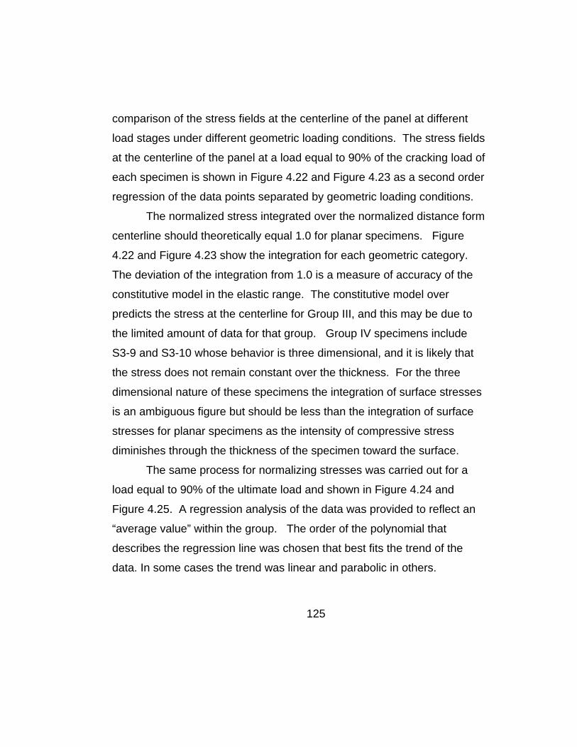
125
comparison of the stress fields at the centerline of the panel at different
load stages under different geometric loading conditions. The stress fields
at the centerline of the panel at a load equal to 90% of the cracking load of
each specimen is shown in Figure 4.22 and Figure 4.23 as a second order
regression of the data points separated by geometric loading conditions.
The normalized stress integrated over the normalized distance form
centerline should theoretically equal 1.0 for planar specimens. Figure
4.22 and Figure 4.23 show the integration for each geometric category.
The deviation of the integration from 1.0 is a measure of accuracy of the
constitutive model in the elastic range. The constitutive model over
predicts the stress at the centerline for Group III, and this may be due to
the limited amount of data for that group. Group IV specimens include
S3-9 and S3-10 whose behavior is three dimensional, and it is likely that
the stress does not remain constant over the thickness. For the three
dimensional nature of these specimens the integration of surface stresses
is an ambiguous figure but should be less than the integration of surface
stresses for planar specimens as the intensity of compressive stress
diminishes through the thickness of the specimen toward the surface.
The same process for normalizing stresses was carried out for a
load equal to 90% of the ultimate load and shown in Figure 4.24 and
Figure 4.25. A regression analysis of the data was provided to reflect an
“average value” within the group. The order of the polynomial that
describes the regression line was chosen that best fits the trend of the
data. In some cases the trend was linear and parabolic in others.
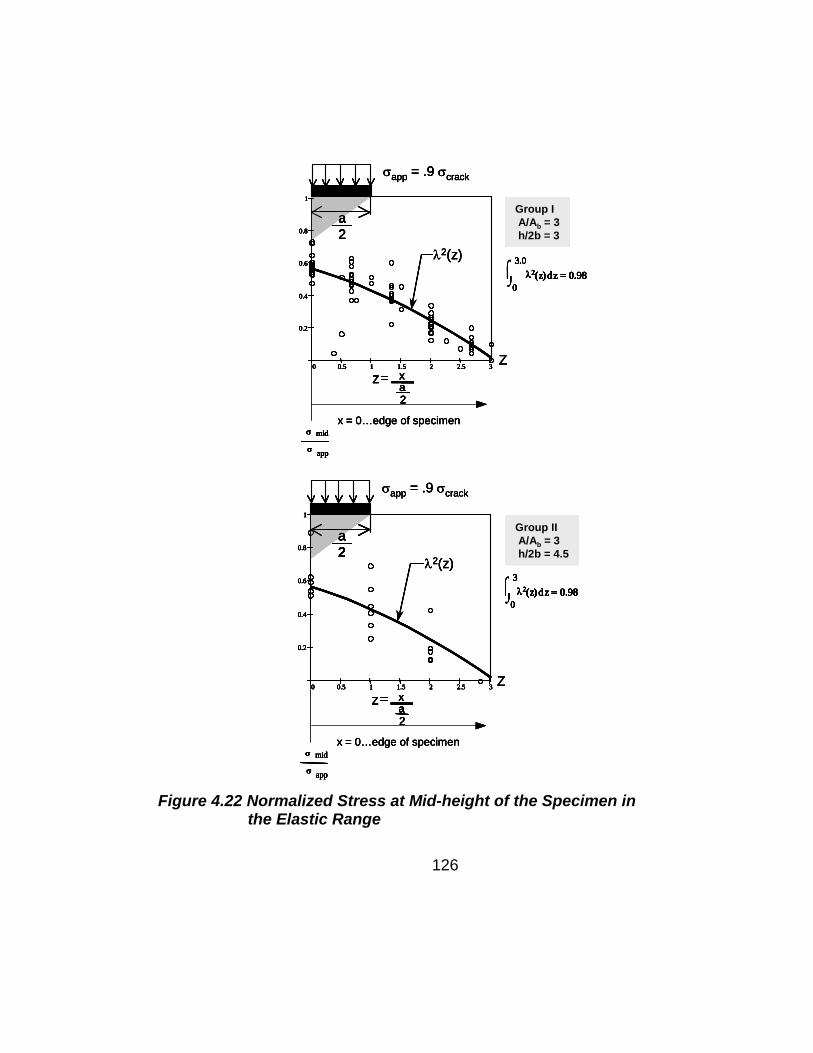
0 0.5 1 1.5 2 2.5 3
0.2
0.4
0.6
0.8
1
Group IA/Ab = 3h/2b = 3
λ2(z)
Z
σapp = .9 σcrack
Z xa2
σ mid
σ app
x = 0…edge of specimen
0
3.0zλ2 z( )
⌠⎮⌡
d 0.98=0
3.0zλ2 z( )
⌠⎮⌡
d 0.98=
a2
0 0.5 1 1.5 2 2.5 3
0.2
0.4
0.6
0.8
1
0 0.5 1 1.5 2 2.5 3
0.2
0.4
0.6
0.8
1
Group IA/Ab = 3h/2b = 3
λ2(z)
Z
σapp = .9 σcrack
Z xa2
Z xa2
σ mid
σ app
σ mid
σ app
x = 0…edge of specimen
0
3.0zλ2 z( )
⌠⎮⌡
d 0.98=0
3.0zλ2 z( )
⌠⎮⌡
d 0.98=
a2a2
0 0.5 1 1.5 2 2.5 3
0.2
0.4
0.6
0.8
1
Group IIA/Ab = 3h/2b = 4.5
λ2(z)
σapp = .9 σcrack
0
3zλ2 z( )
⌠⎮⌡
d 0.98=0
3zλ2 z( )
⌠⎮⌡
d 0.98=
Z xa2
σ mid
σ app
x = 0…edge of specimen
Z
a2
0 0.5 1 1.5 2 2.5 3
0.2
0.4
0.6
0.8
1
0 0.5 1 1.5 2 2.5 3
0.2
0.4
0.6
0.8
1
Group IIA/Ab = 3h/2b = 4.5
λ2(z)
σapp = .9 σcrack
0
3zλ2 z( )
⌠⎮⌡
d 0.98=0
3zλ2 z( )
⌠⎮⌡
d 0.98=
Z xa2
Z xa2
σ mid
σ app
σ mid
σ app
x = 0…edge of specimen
Z
a2a2a2
0 0.5 1 1.5 2 2.5 3
0.2
0.4
0.6
0.8
1
Group IA/Ab = 3h/2b = 3
λ2(z)
Z
σapp = .9 σcrack
Z xa2
σ mid
σ app
x = 0…edge of specimen
0
3.0zλ2 z( )
⌠⎮⌡
d 0.98=0
3.0zλ2 z( )
⌠⎮⌡
d 0.98=
a2
0 0.5 1 1.5 2 2.5 3
0.2
0.4
0.6
0.8
1
0 0.5 1 1.5 2 2.5 3
0.2
0.4
0.6
0.8
1
Group IA/Ab = 3h/2b = 3
λ2(z)
Z
σapp = .9 σcrack
Z xa2
Z xa2
σ mid
σ app
σ mid
σ app
x = 0…edge of specimen
0
3.0zλ2 z( )
⌠⎮⌡
d 0.98=0
3.0zλ2 z( )
⌠⎮⌡
d 0.98=
a2a2
0 0.5 1 1.5 2 2.5 3
0.2
0.4
0.6
0.8
1
Group IIA/Ab = 3h/2b = 4.5
λ2(z)
σapp = .9 σcrack
0
3zλ2 z( )
⌠⎮⌡
d 0.98=0
3zλ2 z( )
⌠⎮⌡
d 0.98=
Z xa2
σ mid
σ app
x = 0…edge of specimen
Z
a2
0 0.5 1 1.5 2 2.5 3
0.2
0.4
0.6
0.8
1
0 0.5 1 1.5 2 2.5 3
0.2
0.4
0.6
0.8
1
Group IIA/Ab = 3h/2b = 4.5
λ2(z)
σapp = .9 σcrack
0
3zλ2 z( )
⌠⎮⌡
d 0.98=0
3zλ2 z( )
⌠⎮⌡
d 0.98=
Z xa2
Z xa2
σ mid
σ app
σ mid
σ app
x = 0…edge of specimen
Z
a2a2a2
Figure 4.22 Normalized Stress at Mid-height of the Specimen in
the Elastic Range
126

0 1 2 3 4 5 6
0.2
0.4
0.6
0.8
1
Group IIIA/Ab = 6h/2b = 3
λ2(z)
σapp = .9 σcrack
0
6zλ2 z( )
⌠⎮⌡
d 1.2=0
6zλ2 z( )
⌠⎮⌡
d 1.2=
a2
Z xa2
σ mid
σ app
x = 0…edge of specimen
Z0 1 2 3 4 5 6
0.2
0.4
0.6
0.8
1
0 1 2 3 4 5 6
0.2
0.4
0.6
0.8
1
Group IIIA/Ab = 6h/2b = 3
λ2(z)
σapp = .9 σcrack
0
6zλ2 z( )
⌠⎮⌡
d 1.2=0
6zλ2 z( )
⌠⎮⌡
d 1.2=
a2a2
Z xa2
σ mid
σ app
x = 0…edge of specimen
Z xa2
Z xa2
σ mid
σ app
σ mid
σ app
x = 0…edge of specimen
Z
0 0.5 1 1.5 2 2.5 3
0.2
0.4
0.6
0.8
1
Group IVA/Ab = 7.5h/2b = 3
λ2(z)
σapp = .9 σcrack
0
3zλ2 z( )
⌠⎮⌡
d 0.74=0
3zλ2 z( )
⌠⎮⌡
d 0.74=
Z xa2
σ mid
σ app
x = 0…edge of specimen
a2
Z0 0.5 1 1.5 2 2.5 3
0.2
0.4
0.6
0.8
1
0 0.5 1 1.5 2 2.5 3
0.2
0.4
0.6
0.8
1
Group IVA/Ab = 7.5h/2b = 3
λ2(z)
σapp = .9 σcrack
0
3zλ2 z( )
⌠⎮⌡
d 0.74=0
3zλ2 z( )
⌠⎮⌡
d 0.74=
Z xa2
σ mid
σ app
x = 0…edge of specimen
Z xa2
Z xa2
σ mid
σ app
σ mid
σ app
x = 0…edge of specimen
a2a2
Z
0 1 2 3 4 5 6
0.2
0.4
0.6
0.8
1
Group IIIA/Ab = 6h/2b = 3
λ2(z)
σapp = .9 σcrack
0
6zλ2 z( )
⌠⎮⌡
d 1.2=0
6zλ2 z( )
⌠⎮⌡
d 1.2=
a2
Z xa2
σ mid
σ app
x = 0…edge of specimen
Z0 1 2 3 4 5 6
0.2
0.4
0.6
0.8
1
0 1 2 3 4 5 6
0.2
0.4
0.6
0.8
1
Group IIIA/Ab = 6h/2b = 3
λ2(z)
σapp = .9 σcrack
0
6zλ2 z( )
⌠⎮⌡
d 1.2=0
6zλ2 z( )
⌠⎮⌡
d 1.2=
a2a2
Z xa2
σ mid
σ app
x = 0…edge of specimen
Z xa2
Z xa2
σ mid
σ app
σ mid
σ app
x = 0…edge of specimen
Z
0 0.5 1 1.5 2 2.5 3
0.2
0.4
0.6
0.8
1
Group IVA/Ab = 7.5h/2b = 3
λ2(z)
σapp = .9 σcrack
0
3zλ2 z( )
⌠⎮⌡
d 0.74=0
3zλ2 z( )
⌠⎮⌡
d 0.74=
Z xa2
σ mid
σ app
x = 0…edge of specimen
a2
Z0 0.5 1 1.5 2 2.5 3
0.2
0.4
0.6
0.8
1
0 0.5 1 1.5 2 2.5 3
0.2
0.4
0.6
0.8
1
Group IVA/Ab = 7.5h/2b = 3
λ2(z)
σapp = .9 σcrack
0
3zλ2 z( )
⌠⎮⌡
d 0.74=0
3zλ2 z( )
⌠⎮⌡
d 0.74=
Z xa2
σ mid
σ app
x = 0…edge of specimen
Z xa2
Z xa2
σ mid
σ app
σ mid
σ app
x = 0…edge of specimen
a2a2
Z
127
Figure 4.23 Normalized Stress at Mid-height of the Specimen in the Elastic Range Cont.

128
The integrated stresses over the normalized distance from
centerline ranged from 0.74 to 1.3 with an under prediction occurring for
unconfined specimens and over predictions for the Group III specimens.
This would indicate that the constitutive model did not capture the
behavior of the stress field after redistribution as well as in the elastic
range. This should be expected, because the exact tensile stress is
difficult to capture past cracking. Figure 4.24 and Figure 4.25 also
display the difference in the stress distributions at the centerline for
confined and unconfined specimens.
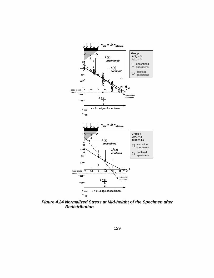
0 0.5 1 1.5 2 2.5 3
0.5
0.25
0.25
0.5
0.75
1
0 0.5 1 1.5 2 2.5 3
0.5
0.25
0.25
0.5
0.75
1
λ(z)unconfined
z
σ mid
σ app
σapp = .9 σultimate
λ(z)confined
a2
x = 0…edge of specimen
regressioncontinuesZ = x
a2
max. tensilestress
Group IA/Ab = 3h/2b = 3
unconfined specimens
confined specimens
0 0.5 1 1.5 2 2.5 3
0.5
0.25
0.25
0.5
0.75
1
0 0.5 1 1.5 2 2.5 3
0.5
0.25
0.25
0.5
0.75
1
λ(z)unconfined
z
σ mid
σ app
σ mid
σ app
σapp = .9 σultimateσapp = .9 σultimate
λ(z)confined
a2a2
x = 0…edge of specimen
regressioncontinuesZ = x
a2
Z = xa2
max. tensilestress
Group IA/Ab = 3h/2b = 3
unconfined specimens
confined specimens
Group IA/Ab = 3h/2b = 3
unconfined specimens
confined specimens
0 0.5 1 1.5 2 2.5 3
0.5
0.25
0.25
0.5
0.75
1
0 0.5 1 1.5 2 2.5 3
0.5
0.25
0.25
0.5
0.75
1
σapp = .9 σultimate
λ(z)unconfined
λ2(z)confined
max. tensilestress
regressioncontinues
x = 0…edge of specimen
z
σ mid
σ app
Z = xa2
a2
Group IIA/Ab = 3h/2b = 4.5
unconfined specimens
confined specimens
0 0.5 1 1.5 2 2.5 3
0.5
0.25
0.25
0.5
0.75
1
0 0.5 1 1.5 2 2.5 3
0.5
0.25
0.25
0.5
0.75
1
σapp = .9 σultimate
λ(z)unconfined
λ2(z)confined
max. tensilestress
regressioncontinues
x = 0…edge of specimen
z
σ mid
σ app
σ mid
σ app
Z = xa2
Z = xa2
a2a2
Group IIA/Ab = 3h/2b = 4.5
unconfined specimens
confined specimens
Group IIA/Ab = 3h/2b = 4.5
unconfined specimens
confined specimens
Figure 4.24 Normalized Stress at Mid-height of the Specimen after
Redistribution
129
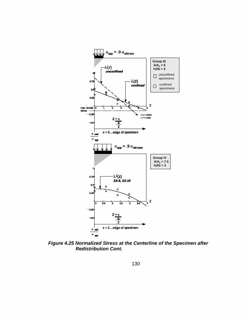
σapp = .9 σultimate
0 1 2 3 4 5 6
0.5
0.25
0.25
0.5
0.75
1
0 1 2 3 4 5 6
0.5
0.25
0.25
0.5
0.75
1
λ(z)unconfined
λ(z)confined
Group IIIA/Ab = 6h/2b = 3
unconfined specimens
confined specimens
regressioncontinues
max. tensilestress
σ mid
σ app
x = 0…edge of specimen
Z = xa2
Z
σapp = .9 σultimate
0 1 2 3 4 5 6
0.5
0.25
0.25
0.5
0.75
1
0 1 2 3 4 5 6
0.5
0.25
0.25
0.5
0.75
1
λ(z)unconfined
λ(z)confined
Group IIIA/Ab = 6h/2b = 3
unconfined specimens
confined specimens
Group IIIA/Ab = 6h/2b = 3
unconfined specimens
confined specimens
regressioncontinues
max. tensilestress
σ mid
σ app
x = 0…edge of specimenσ mid
σ app
σ mid
σ app
x = 0…edge of specimen
Z = xa2
Z = xa2
Z
σapp = .9 σultimate
0 0.5 1 1.5 2 2.5 3
0.5
0.25
0.25
0.5
0.75
1
0 0.5 1 1.5 2 2.5 3
0.5
0.25
0.25
0.5
0.75
1
λ2(z)S3-9, S3-10
Group IVA/Ab = 7.5h/2b = 3
σ mid
σ app
x = 0…edge of specimen
Z = xa2
Z
σapp = .9 σultimate
0 0.5 1 1.5 2 2.5 3
0.5
0.25
0.25
0.5
0.75
1
0 0.5 1 1.5 2 2.5 3
0.5
0.25
0.25
0.5
0.75
1
λ2(z)S3-9, S3-10
Group IVA/Ab = 7.5h/2b = 3
Group IVA/Ab = 7.5h/2b = 3
σ mid
σ app
σ mid
σ app
x = 0…edge of specimen
Z = xa2
Z = xa2
Z
σapp = .9 σultimate
0 1 2 3 4 5 6
0.5
0.25
0.25
0.5
0.75
1
0 1 2 3 4 5 6
0.5
0.25
0.25
0.5
0.75
1
λ(z)unconfined
λ(z)confined
Group IIIA/Ab = 6h/2b = 3
unconfined specimens
confined specimens
regressioncontinues
max. tensilestress
σ mid
σ app
x = 0…edge of specimen
Z = xa2
Z
σapp = .9 σultimate
0 1 2 3 4 5 6
0.5
0.25
0.25
0.5
0.75
1
0 1 2 3 4 5 6
0.5
0.25
0.25
0.5
0.75
1
λ(z)unconfined
λ(z)confined
Group IIIA/Ab = 6h/2b = 3
unconfined specimens
confined specimens
Group IIIA/Ab = 6h/2b = 3
unconfined specimens
confined specimens
regressioncontinues
max. tensilestress
σ mid
σ app
x = 0…edge of specimenσ mid
σ app
σ mid
σ app
x = 0…edge of specimen
Z = xa2
Z = xa2
Z
σapp = .9 σultimate
0 0.5 1 1.5 2 2.5 3
0.5
0.25
0.25
0.5
0.75
1
0 0.5 1 1.5 2 2.5 3
0.5
0.25
0.25
0.5
0.75
1
λ2(z)S3-9, S3-10
Group IVA/Ab = 7.5h/2b = 3
σ mid
σ app
x = 0…edge of specimen
Z = xa2
Z
σapp = .9 σultimate
0 0.5 1 1.5 2 2.5 3
0.5
0.25
0.25
0.5
0.75
1
0 0.5 1 1.5 2 2.5 3
0.5
0.25
0.25
0.5
0.75
1
λ2(z)S3-9, S3-10
Group IVA/Ab = 7.5h/2b = 3
Group IVA/Ab = 7.5h/2b = 3
σ mid
σ app
σ mid
σ app
x = 0…edge of specimen
Z = xa2
Z = xa2
Z
Figure 4.25 Normalized Stress at the Centerline of the Specimen after
Redistribution Cont.
130

The gradient of the stress distribution of confined specimens is less
then the gradient of the stress distribution of unconfined specimens
ultimately contributing to larger tensile stress at the edge of the specimen.
The spread of compressive stresses can be taken as the ratio of the
distance from the edge of the bearing plate (1) to the point where the
regression line crosses the distance axis divided by the half the height of
the specimen normalized with respect to the half the bearing plate
dimension. These ratios are displayed in Table 4.1.
Table 4.1 Spread of Compressive Stress
X
X
X
X
unconfinedconfined
8:15GROUP IV
11:24GROUP III
5:8XGROUP III
4:15GROUP II
7:12XGROUP II
5:12GROUP I
1:2XGROUP I
AngleFailure mechanismGroup
X
X
X
X
unconfinedconfined
8:15GROUP IV
11:24GROUP III
5:8XGROUP III
4:15GROUP II
7:12XGROUP II
5:12GROUP I
1:2XGROUP I
AngleFailure mechanismGroup
131
The ratios shown in Table 4.1 convert to angle between 14 degrees
and 32 degrees. The steepest angle is that of the Group II unconfined
specimens of which there were three specimens that exhibited an
unconfined failure mechanism, two of which had confining reinforcing at
the node which altered the stress distribution at the centerline of the
132
specimen and therefore were not included. The exclusion of specimens
S2-4 and S1-5 left only specimen S1-2 which contained no reinforcing.
The steep angle is consistent with amount of reinforcement present in that
the angle tends toward zero with respect to vertical as the amount of
reinforcing steel provided decreases. In general, specimens with sufficient
reinforcement to produce a confined failure of crushing at or around the
nodal area had a characteristic spread of compression at a rate of 1
horizontal unit to 2 vertical units or larger. Unconfined specimens
exhibited a slightly smaller spread of compressive stresses leading to
greater tensile stress at the outer edge of the specimen. This variation
between confined and unconfined specimens stayed constant between
geometric groups; however, as the ratio of the loaded surface to bearing
plate increased in Group III the spread of compression also increased.
4.5.1 Summary of Results Obtained from Strain on the Concrete
Surface of the Specimens
The stress distribution across the centerline of a specimen was
reasonably attainable with limited amounts of concrete surface gauges
placed at regular intervals along the centerline of the specimen. The
stress distribution across the centerline depended on the load stage
considered, the amount of reinforcement provided and the geometric
conditions of loading. At load stages after cracking, tensile stresses
developed at the edge of the specimen and the stresses were greater in
specimens that exhibited an unconfined failure mechanism of a tensile
failure at a plane further away from the node than the confined failure of

133
crushing of concrete at and around the nodal area. The spreading of the
compressive stress varies by the geometric conditions of loading and the
reinforcement provided; however the spread may reasonably be assumed
at a rate of 1 horizontal unit to 2 vertical units as depicted in Appendix A of
the ACI 318-02.
134
5.0 ANALYSIS OF THE RESULTS AND CONCLUSIONS
5.1 DESCRIBING THE BEHAVIOR WITH EMPIRICAL METHODS
As mentioned in Chapter 4, specimens analogous to those
fabricated in the experimental program described in Chapter 3 have been
investigated by many researchers [11], [13], [14], [21], [22], [34], [35], [36],
[39], [44], [50]. The result of many of these investigations has been the
development of empirical relations based on regression analyses of the
parameters considered in each investigation. For example Niyogi [34]
presented an equation for the bearing capacity as a function of the ratios
of bearing plate dimensions to that of the adjacent dimensions of the
loaded surface. Roberts [39] used a semi-empirical equation to describe
the behavior of specimens in which the loaded area was smaller than that
of the supporting surface and included an empirical term as well as a term
describing the behavior of confined concrete in the presence of
rectangular ties or spirals. An empirical relationship for the bearing
capacity of the specimens tested in the experimental program reported
here is also reported in this chapter.
The main parameters affecting the behavior of the specimens
tested were: the amount of reinforcement provided, the ratio of the cross-
sectional area to that of the bearing plate area (A/Ab), and the height of
the specimen to that of thickness of the specimen (h/2b). As seen from
Figure 4.7, the width of the compression field at the centerline of the
specimen was a function of the amount of reinforcement provided.
Relating the width of the compression field at midheight of the specimen
(which is dependent on the amount of reinforcement provided) to the area
135
of the loaded surface indirectly combines two parameters. An empirical
equation was produced from regression analyses of the parameters
mentioned previously and a comparison of the regression analyses to the
test results is illustrated in Figure 5.1. Figures 5.2 and 5.3 compare the
empirical equation presented by Niyogi [34] and semi-empirical equation
presented by Roberts [39] to the test results. The efficiency factor of
concrete defined as the ultimate stress under the bearing plate normalized
to the compressive strength of concrete (νe) is the parameter by which the
comparison of empirical equations to test results was made.
It can be seen by Figures 5.1, 5.2, and 5.3 that empirical equations
correlate quite well in some instances and rather poorly in others. The
variation is due to the fact that the empirical relations are modeled after a
specific set of specimens and geometric loading conditions beyond which
the parameters used in developing the empirical relations may not be
directly applicable.
It was not the intent of this research project to develop empirical
relations for the bearing capacity of concrete specimens loaded over a
limited surface area; however, empirical relations and comparisons with
the test data are presented here to illustrate an important point: strut-and-
tie models can be used to describe the behavior of concrete elements that
have previously been unexplainable by classical methods of analysis.
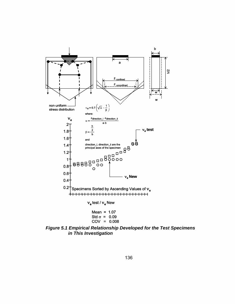
νe
Specimens Sorted by Ascending Values of νe
νe test
νe New
νe test / νe New
Mean = 1.07Std σ = 0.09COV = 0.008
h/2
w
b
z confined
z unconfined
a
νe 0.7 α1β
−⎛⎜⎝
⎞⎟⎠
⋅
where:
αzdirection_i zdirection_ii⋅
a b⋅
β
h
2
b
and
direction_i, direction_ii are the principal axes of the specimen
non-uniformstress distribution
0.2
0.4
0.6
0.8
1
1.2
1.4
1.6
1.8
2
w
Figure 5.1 Empirical Relationship Developed for the Test Specimens
in This Investigation
136
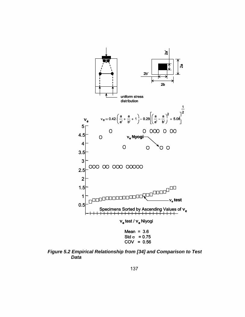
0.5
1
1.5
2
2.5
3
3.5
4
4.5
5νe
Specimens Sorted by Ascending Values of νe
νe test
νe Nyogi
uniform stress distribution
2a
2a’
2b
2b’
νe test / νe Niyogi
Mean = 3.6Std σ = 0.75COV = 0.56
νe 0.42aa'
ab'
+ 1+⎛⎜⎝
⎞⎟⎠
⋅ 0.29aa'
ab'
−⎛⎜⎝
⎞⎟⎠
25.06+
⎡⎢⎣
⎤⎥⎦
1
2
−_
0.5
1
1.5
2
2.5
3
3.5
4
4.5
5νe
Specimens Sorted by Ascending Values of νe
νe test
νe Nyogi
uniform stress distribution
2a
2a’
2b
2b’
νe test / νe Niyogi
Mean = 3.6Std σ = 0.75COV = 0.56
νe 0.42aa'
ab'
+ 1+⎛⎜⎝
⎞⎟⎠
⋅ 0.29aa'
ab'
−⎛⎜⎝
⎞⎟⎠
25.06+
⎡⎢⎣
⎤⎥⎦
1
2
−_
0.5
1
1.5
2
2.5
3
3.5
4
4.5
5νe
Specimens Sorted by Ascending Values of νe
νe test
νe Nyogi
uniform stress distribution
2a
2a’
2b
2b’
2a
2a’
2b
2b’
νe test / νe Niyogi
Mean = 3.6Std σ = 0.75COV = 0.56
νe 0.42aa'
ab'
+ 1+⎛⎜⎝
⎞⎟⎠
⋅ 0.29aa'
ab'
−⎛⎜⎝
⎞⎟⎠
25.06+
⎡⎢⎣
⎤⎥⎦
1
2
−_
Figure 5.2 Empirical Relationship from [34] and Comparison to Test
Data
137
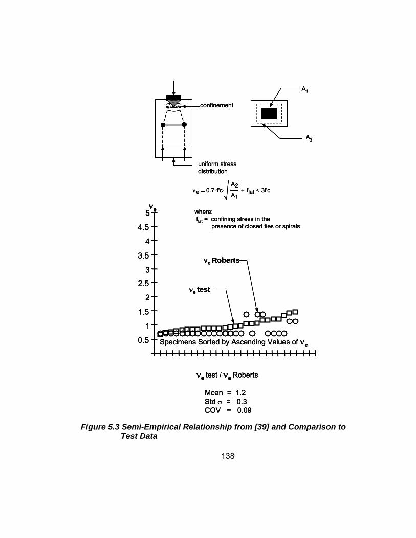
0.5
1
1.5
2
2.5
3
3.5
4
4.5
5νe
Specimens Sorted by Ascending Values of νe
νe test
νe Roberts
uniform stress distribution
νe test / νe Roberts
Mean = 1.2Std σ = 0.3COV = 0.09
confinement
A1
A2
where:flat = confining stress in the
presence of closed ties or spirals
νe 0.7 f'c⋅A2
A1⋅ flat+ 3f'c≤
_
0.5
1
1.5
2
2.5
3
3.5
4
4.5
5νe
Specimens Sorted by Ascending Values of νe
νe test
νe Roberts
uniform stress distribution
νe test / νe Roberts
Mean = 1.2Std σ = 0.3COV = 0.09
confinement
A1
A2
where:flat = confining stress in the
presence of closed ties or spirals
νe 0.7 f'c⋅A2
A1⋅ flat+ 3f'c≤
_
0.5
1
1.5
2
2.5
3
3.5
4
4.5
5νe
Specimens Sorted by Ascending Values of νe
νe test
νe Roberts
uniform stress distribution
νe test / νe Roberts
Mean = 1.2Std σ = 0.3COV = 0.09
confinement
A1
A2
where:flat = confining stress in the
presence of closed ties or spirals
νe 0.7 f'c⋅A2
A1⋅ flat+ 3f'c≤
_
Figure 5.3 Semi-Empirical Relationship from [39] and Comparison to
Test Data
138
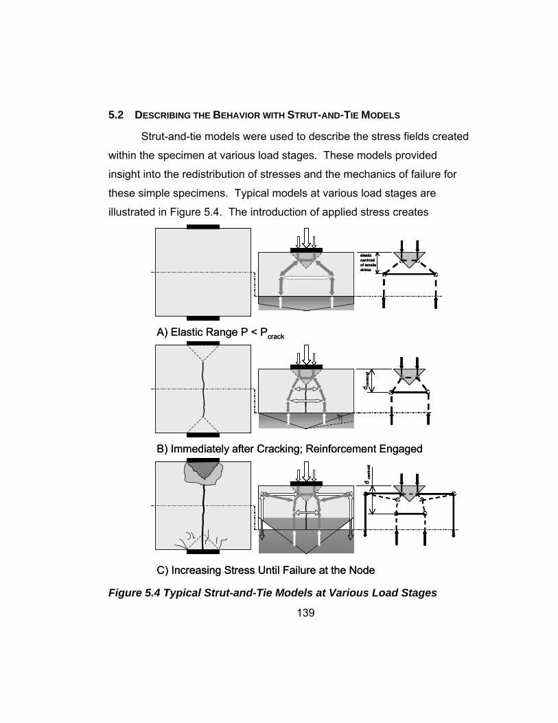
5.2 DESCRIBING THE BEHAVIOR WITH STRUT-AND-TIE MODELS
Strut-and-tie models were used to describe the stress fields created
within the specimen at various load stages. These models provided
insight into the redistribution of stresses and the mechanics of failure for
these simple specimens. Typical models at various load stages are
illustrated in Figure 5.4. The introduction of applied stress creates
A) Elastic Range P < Pcrack
B) Immediately after Cracking; Reinforcement Engaged
C) Increasing Stress Until Failure at the Node
elastic centroidof tensilestress
elastic centroidof tensilestress
d cen
troid
d cen
troid
d ce
ntro
idd
cent
roid
A) Elastic Range P < Pcrack
B) Immediately after Cracking; Reinforcement Engaged
C) Increasing Stress Until Failure at the Node
elastic centroidof tensilestress
elastic centroidof tensilestress
d cen
troid
d cen
troid
d ce
ntro
idd
cent
roid
Figure 5.4 Typical Strut-and-Tie Models at Various Load Stages
139

a region of biaxial compression in planar elements and tri-axial
compression in three-dimensional elements directly under the bearing
plate. In reality no structural concrete members are truly planar and have
some finite thickness in the third dimension leading to a tri-axial state of
compression at the midpoint of the thickness of the element, which
gradually reduces to a state of biaxial compression at the surface of the
element. Such nodal regions are commonly referred to as hydrostatic
nodes and to satisfy equilibrium, stresses perpendicular to the applied
stress must equal the applied stress. The equilibrium of sresses
geometrically forms an isosceles triangle with a height equal to half the
width, of which, the stresses are equal on all sides. The geometry of
these nodes was continually substantiated by the geometry of the intact
concrete under the bearing plate of the specimens within the experimental
program. As a result of the stress state within the nodal region,
compressive stresses propagate from the node initially at 45 degrees. To
satisfy equilibrium, elements at the interior of the specimen, defined as the
region enclosed by a line drawn at 45 degrees from the edge of the
bearing area to the edge of the specimen, are subjected to some degree
of transverse tensile stress as shown in Figure 5.5.
Figure 5.5 Stress Fields for a Typical Specimen Adapted from [33]
140

141
Once the specimen cracks, the transverse stiffness provided by the
uncracked concrete in tension disappears, and a significantly reduced
stiffness provided by the reinforcement replaces the initial concrete
stiffness. The net effect is the movement of the centroid of compressive
stresses to the centerline of the section.
Consider a free-body diagram composed of one symmetrical
quadrant of an uncracked specimen (Figure 5.6 A). The stress present at
the vertical face of the hydrostatic node is equal to the bearing stress and
is also equal to the tensile stress developed within the concrete plus a
negligible amount of tensile stress provided by the reinforcement. The
struts anchoring the tension in the concrete and the tension in the
reinforcement must provide a force equal the resultant of the compressive
stresses at the horizontal and vertical faces of the node. Summing the
moments about point X in Figure 5.6 A yields a system of nonlinear
equations with two unknowns which are the angles θ and φ. There is no
unique solution to this system of equations. Each solution will result in the
same stress distribution across the mid-height of the panel depending on
the tension force assigned to the reinforcement. However, some solutions
are more suitable than others. Solutions that result in angles of φ that
deviate strongly from the elastic stress distribution, as well as, solutions
that that result in the concrete tension component being much larger than
the tension capacity of concrete calculated by the area of concrete
extending from the node to the midheight of the section should also be
avoided. The elastic strut-and-tie model shown in Figure 5.6 A) is the
culmination of two sub-models that divides the load carried by each sub-
model based on the angle θ chosen from the range of possible solutions.
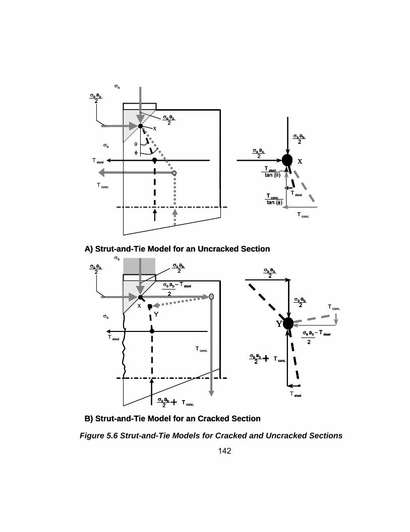
σb ab2 T conc.
Y
σb ab2
σb ab2
σb ab – T steel
2
T steel
σb
T conc.
xσb ab
2
σb ab2
T steel
T steel
.
σb
θφ
x
σb
σb ab2
T conc.
σb ab2
T steel
T conc.
xσb
σb ab2
σb ab – T steel
2
σb ab2 T conc.
σb ab2
Y
T steel tan (θ)
T conc. tan (φ)
A) Strut-and-Tie Model for an Uncracked Section
B) Strut-and-Tie Model for an Cracked Section
T conc.
σb ab2 T conc.
Y
σb ab2
σb ab2
σb ab – T steel
2
T steel
σb ab2 T conc.
σb ab2
σb ab2 T conc.
Y
σb ab2
σb ab2
σb ab2
σb ab2
σb ab – T steel
2
σb ab – T steel
2
T steel
σb
T conc.
xσb ab
2σb ab
2
σb ab2
σb ab2
T steel
T steel
.
σb
θφ
x
σb
σb ab2
σb ab2
T conc.
σb ab2
σb ab2
T steel
T conc.
xσb
σb ab2
σb ab2
σb ab – T steel
2
σb ab – T steel
2
σb ab2 T conc.
σb ab2
σb ab2 T conc.
σb ab2
σb ab2
Y
T steel tan (θ)T steel tan (θ)
T conc. tan (φ)T conc. tan (φ)
A) Strut-and-Tie Model for an Uncracked Section
B) Strut-and-Tie Model for an Cracked Section
T conc.
Figure 5.6 Strut-and-Tie Models for Cracked and Uncracked Sections
142

T steel
θ
xT steel
T steel tan (θ)
T steel tan (θ)
T steel
θ
xT steel
T steel tan (θ)T steel tan (θ)
T steel tan (θ)T steel tan (θ)
.
φ
x
T conc.
T conc.
T conc. tan (φ)
T conc. tan (φ)
.
φ
x
T conc.
T conc.
T conc. tan (φ)T conc. tan (φ)
T conc. tan (φ)T conc. tan (φ)
T steel
.
σb
θφ
x
σb
σb ab2
T conc.
σb ab2
T steel
.
σb
θφ
x
σb
σb ab2
σb ab2
T conc.
σb ab2
σb ab2
NODE
a2
a 2
T steel tan (θ)
a2
T conc. tan (φ)
a2
T steel
a2
T conc.
a2
σb
σb
NODE
a2a2
a 2a 2
T steel tan (θ)
a2
T steel tan (θ)T steel tan (θ)
a2a2
T conc. tan (φ)
a2
T conc. tan (φ)T conc. tan (φ)
a2a2
T steel
a2
T steel
a2a2
T conc.
a2
T conc.
a2a2
σb
σb
Figure 5.7 Separation of Sub-Models in the Elastic Range
143
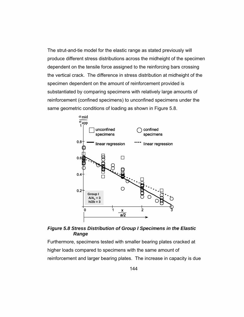
The strut-and-tie model for the elastic range as stated previously will
produce different stress distributions across the midheight of the specimen
dependent on the tensile force assigned to the reinforcing bars crossing
the vertical crack. The difference in stress distribution at midheight of the
specimen dependent on the amount of reinforcement provided is
substantiated by comparing specimens with relatively large amounts of
reinforcement (confined specimens) to unconfined specimens under the
same geometric conditions of loading as shown in Figure 5.8.
0 1 2 3
0.2
0.4
0.6
0.8
1unconfinedspecimens
linear regression
confinedspecimens
linear regression
Group IA/Ab = 3h/2b = 3
σmidσapp
xa/2
0 1 2 3
0.2
0.4
0.6
0.8
1unconfinedspecimens
linear regression
confinedspecimens
linear regression
Group IA/Ab = 3h/2b = 3
σmidσapp
xa/2xa/2
Figure 5.8 Stress Distribution of Group I Specimens in the Elastic
Range Furthermore, specimens tested with smaller bearing plates cracked at
higher loads compared to specimens with the same amount of
reinforcement and larger bearing plates. The increase in capacity is due
144
145
to the increase of the concrete tensile component created from reducing
the size of the node.
Once the section cracks, the strut-and-tie model changes
significantly as displayed in Figure 5.6 B. The concrete tensile component
disappears yet the compressive stresses at the vertical face of the node
are still present. The loss of the concrete tensile capacity results in large
tensile stress fields at the edges of the specimen which are modeled as
tensile forces parallel and perpendicular to the load applied. The tensile
stresses at the edge of the specimen act normal to the plane of the model
shown in Figure 5.6 B within the thickness of the specimen causing
splitting failures as seen in the specimens tested and shown in Figure 4.6.
Anchoring the splitting forces is a strut whose magnitude is determined by
the tensile forces at the top face and side face of the specimen. A
numerical example of producing a typical strut and tie model including the
tensile forces at top edge and side edge of the specimen is presented in
Figure 5.9. The splitting forces developed within the specimens are
analogous to other structural elements where a force couple is not present
to restrain the compressive stresses of the vertical face of a singular node.
Two examples of the splitting force being restrained by force couples are
the uncracked specimen in Figure 5.6 A where the compressive force is
resisted by the tensile force in the concrete and a node in the compression
zone a beam where the stress at the vertical face of the node is resisted
by the force couple due to bending.
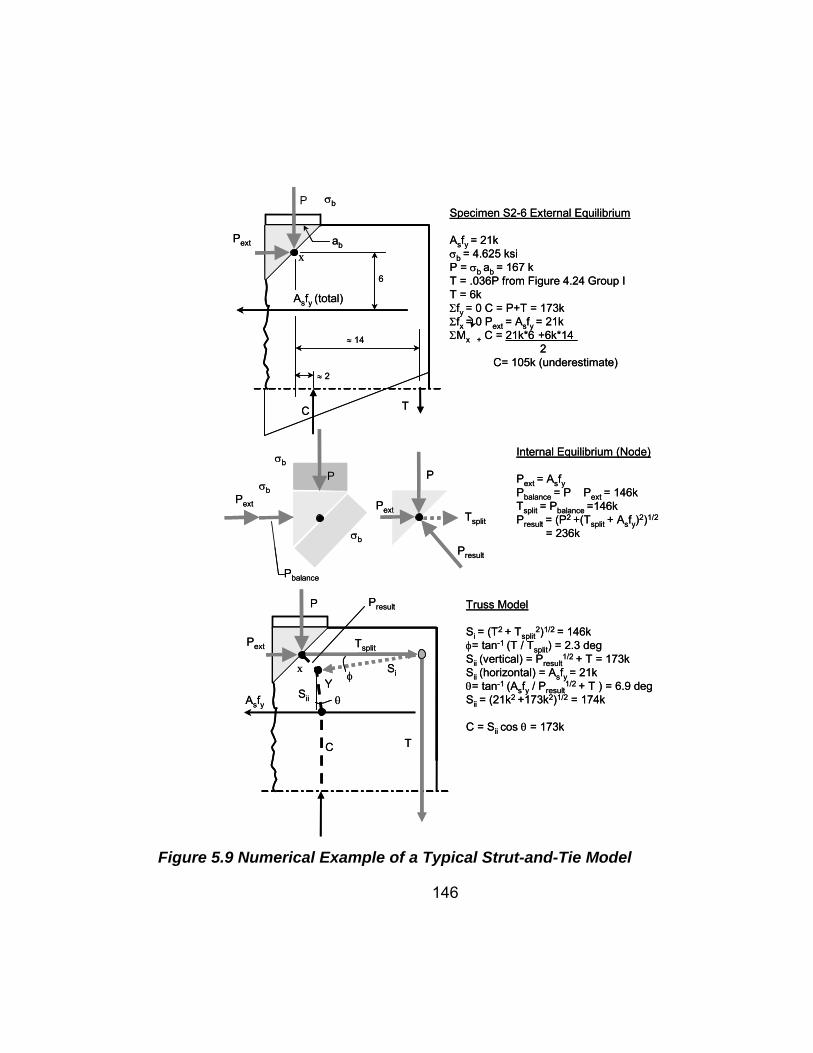
x
xY
C T
σbSpecimen S2-6 External Equilibrium
Asfy = 21kσb = 4.625 ksiP = σb ab = 167 kT = .036P from Figure 4.24 Group IT = 6kΣfy = 0 C = P+T = 173kΣfx = 0 Pext = Asfy = 21kΣMx + C = 21k*6�+6k*14�
2�C= 105k (underestimate)
P
Asfy (total)
Pext
≈ 2�
≈ 14�
6�
σb
σbPext
P
Pbalance
ab
σb
Internal Equilibrium (Node)
Pext = Asfy Pbalance = P �Pext = 146kTsplit = Pbalance =146kPresult = (P2 +(Tsplit + Asfy)2)1/2
= 236k
P
Tsplit
Tsplit
TC
Presult
P
Asfy
Pext
Presult
Si
Sii
Pext
Truss Model
Si = (T2 + Tsplit2)1/2 = 146k
φ= tan-1 (T / Tsplit) = 2.3 degSii (vertical) = Presult
1/2 + T = 173kSii (horizontal) = Asfy = 21kθ= tan-1 (Asfy / Presult
1/2 + T ) = 6.9 degSii = (21k2 +173k2)1/2 = 174k
C = Sii cos θ = 173k
φ
θ
Figure 5.9 Numerical Example of a Typical Strut-and-Tie Model
146

Muttoni [33] shows one such example of splitting forces in the case
of a pre-tensioned beam shown in Figure 5.9.
splitting forcessplitting forces
Figure 5.10 Splitting Forces within a Pre-Tensioned Beam from [33]
Sanders [44] did not include the splitting forces shown in Figure 5.9
in the models he proposed for his anchorage specimens which were
present in the specimens in which a crack propagated to the base
negating the uniform stress distribution assumed within the models,
instead, he based his models solely on the reinforcement within the
section as shown in Figure 5.11. Sanders’ models were conservative and
provided good correlation with the test data gathered within his
experimental program; however, his models did not reflect the behavior of
unreinforced specimens.
147
The strut-and-tie models presented followed Schlaich’s [46]
approach which assumed that sub-models could be created that divided
the load in any manner desired by the designer with the caveat that
equilibrium most be satisfied. The strut-and-tie model presented for the
cracked section split the force applied to the vertical face of the node into
two components; one consisted of the force couple of the tension steel,
while the other component was the remainder of the force at the node
transferred into a splitting tension as shown Figure 5.12.

T1
T2
T3
h/4 TYP
P/2P/2a/4
dcentroidα
tan α( )h4
a4
−
dcentroida4
−
σb
T steel
T conc.
xσb
σb ab2
σb ab – T steel
2
σb ab2 T conc.
σb ab2
Y
A) Sanders’ Strut-and Tie Models Used for End Anchorage Specimens
B) Strut-and-Tie Model for an Unreinforced Specimen
T1
T2
T3
h/4 TYP
P/2P/2a/4
dcentroidα
tan α( )h4
a4
−
dcentroida4
−
T1
T2
T3
h/4 TYP
P/2P/2a/4
dcentroidα
T1
T2
T3
h/4 TYP
P/2P/2a/4
dcentroidα
tan α( )h4
a4
−
dcentroida4
−
σb
T steel
T conc.
xσb
σb ab2
σb ab – T steel
2
σb ab2 T conc.
σb ab2
Y
σb
T steel
T conc.
xσb
σb ab2
σb ab2
σb ab – T steel
2
σb ab – T steel
2
σb ab2 T conc.
σb ab2
σb ab2 T conc.
σb ab2
σb ab2
Y
A) Sanders’ Strut-and Tie Models Used for End Anchorage Specimens
B) Strut-and-Tie Model for an Unreinforced Specimen Figure 5.11 Comparison of Strut-and-Tie Models with [44]
148
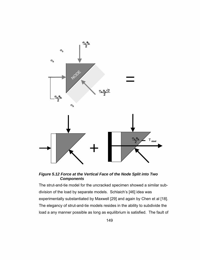
σb
σb ab2
NODE
T steelσb ab
2
σb
σb
σb ab2
σb ab√22
σb
σb ab2
σb ab2
NODE
T steelσb ab
2σb ab
2
σb
σb
σb ab2
σb ab2
σb ab√22
σb ab√22
Figure 5.12 Force at the Vertical Face of the Node Split into Two Components
The strut-and-tie model for the uncracked specimen showed a similar sub-
division of the load by separate models. Schlaich’s [46] idea was
experimentally substantiated by Maxwell [29] and again by Chen et al [18].
The elegancy of strut-and-tie models resides in the ability to subdivide the
load a any manner possible as long as equilibrium is satisfied. The fault of
149
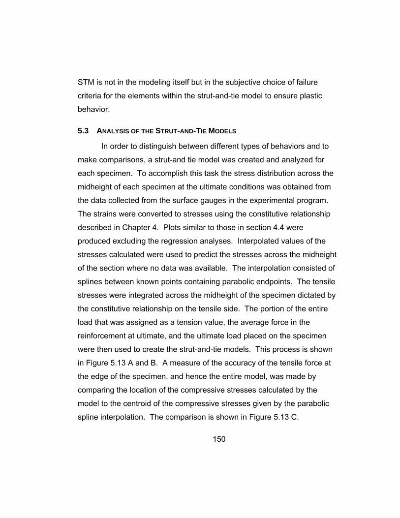
150
STM is not in the modeling itself but in the subjective choice of failure
criteria for the elements within the strut-and-tie model to ensure plastic
behavior.
5.3 ANALYSIS OF THE STRUT-AND-TIE MODELS
In order to distinguish between different types of behaviors and to
make comparisons, a strut-and tie model was created and analyzed for
each specimen. To accomplish this task the stress distribution across the
midheight of each specimen at the ultimate conditions was obtained from
the data collected from the surface gauges in the experimental program.
The strains were converted to stresses using the constitutive relationship
described in Chapter 4. Plots similar to those in section 4.4 were
produced excluding the regression analyses. Interpolated values of the
stresses calculated were used to predict the stresses across the midheight
of the section where no data was available. The interpolation consisted of
splines between known points containing parabolic endpoints. The tensile
stresses were integrated across the midheight of the specimen dictated by
the constitutive relationship on the tensile side. The portion of the entire
load that was assigned as a tension value, the average force in the
reinforcement at ultimate, and the ultimate load placed on the specimen
were then used to create the strut-and-tie models. This process is shown
in Figure 5.13 A and B. A measure of the accuracy of the tensile force at
the edge of the specimen, and hence the entire model, was made by
comparing the location of the compressive stresses calculated by the
model to the centroid of the compressive stresses given by the parabolic
spline interpolation. The comparison is shown in Figure 5.13 C.
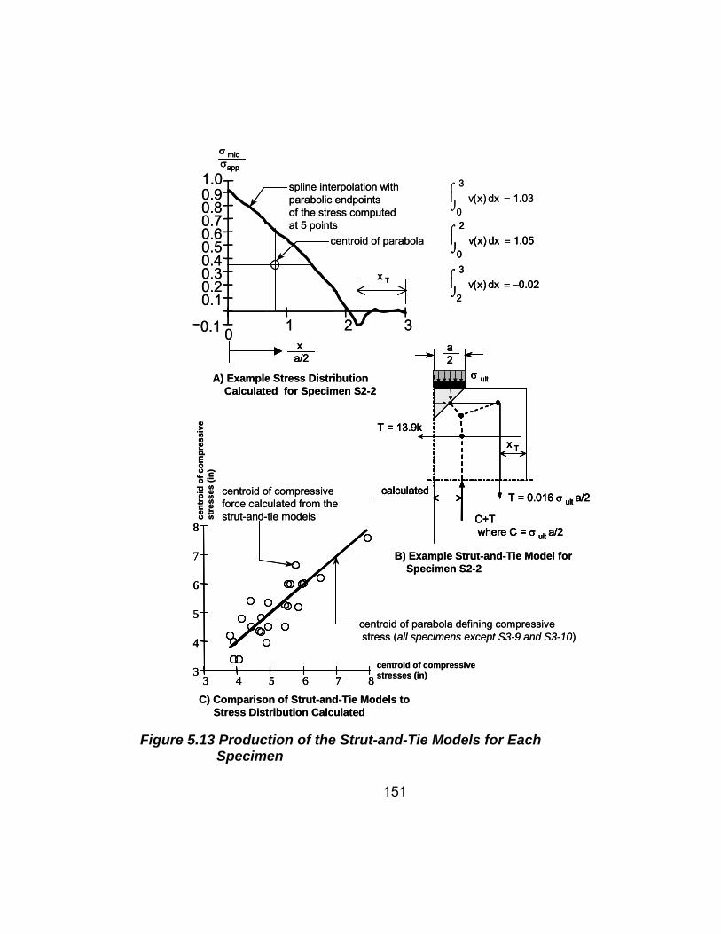
0 1 2 30.1
0.10.20.30.40.50.60.70.80.91.0
0
3v x( )
⌠⎮⌡
dx 1.03=
0
2v x( )
⌠⎮⌡
dx 1.05=
2
3v x( )
⌠⎮⌡
dx 0.02−=
spline interpolation with parabolic endpointsof the stress computedat 5 points
xa/2
σ mid σapp
3 4 5 6 7 83
4
5
6
7
8
centroid of parabola
x T
a2
σ ult
T = 0.016 σ ult a/2
T = 13.9k
C+Twhere C = σ ult a/2
calculated
x T
A) Example Stress Distribution Calculated for Specimen S2-2
B) Example Strut-and-Tie Model for Specimen S2-2
centroid of parabola defining compressivestress (all specimens except S3-9 and S3-10)
centroid of compressive force calculated from the strut-and-tie models
C) Comparison of Strut-and-Tie Models to Stress Distribution Calculated
centroid of compressive stresses (in)
cent
roid
of c
ompr
essi
ve
stre
sses
(in)
0 1 2 30.1
0.10.20.30.40.50.60.70.80.91.0
0
3v x( )
⌠⎮⌡
dx 1.03=
0
2v x( )
⌠⎮⌡
dx 1.05=0
2v x( )
⌠⎮⌡
dx 1.05=
2
3v x( )
⌠⎮⌡
dx 0.02−=2
3v x( )
⌠⎮⌡
dx 0.02−=
spline interpolation with parabolic endpointsof the stress computedat 5 points
xa/2x
a/2
σ mid σapp
σ mid σapp
3 4 5 6 7 83
4
5
6
7
8
3 4 5 6 7 83
4
5
6
7
8
centroid of parabola
x T
a2
σ ult
T = 0.016 σ ult a/2
T = 13.9k
C+Twhere C = σ ult a/2
calculated
x T
a2a2
σ ult
T = 0.016 σ ult a/2
T = 13.9k
C+Twhere C = σ ult a/2
calculated
x T
σ ult
T = 0.016 σ ult a/2
T = 13.9k
C+Twhere C = σ ult a/2
calculated
x T
A) Example Stress Distribution Calculated for Specimen S2-2
B) Example Strut-and-Tie Model for Specimen S2-2
centroid of parabola defining compressivestress (all specimens except S3-9 and S3-10)
centroid of compressive force calculated from the strut-and-tie models
C) Comparison of Strut-and-Tie Models to Stress Distribution Calculated
centroid of compressive stresses (in)
cent
roid
of c
ompr
essi
ve
stre
sses
(in)
Figure 5.13 Production of the Strut-and-Tie Models for Each
Specimen
151

152
The mean difference between the centroid of the compressive stresses
calculated by the model and the centroid of compressive stresses given by
the stress distribution was .44 inches with a standard deviation of 0.3
inches. These values indicate that the tensile forces at the edge of the
specimens were calculated fairly well in light of the fact that capturing the
tensile stress in concrete is extremely difficult due to factors mentioned in
section 4.6.
The result of the analysis shows that the type of failure mechanism
associated with each specimen has a strong correlation with the location
of point Y in Figure 5.6 B. Unconfined failures are typified by larger
distances of point Y from the singular node, or in other terms, a longer
strut length Siii as shown in Figure 5.14. As the percentage of steel
increased, the length of strut Siii steadily decreased edging closer and
closer to the singular node. The length of the critical strut Siii was
dependent on the angle of the strut that anchors the deviation of the
splitting force around the corner of the specimen as shown in Figure 5.9,
and the relative distance from the node to the anchoring point of the
tensile forces (dT/ab in Figure 5.14). As the steel yields the steel force
remains nearly constant; however the horizontal splitting force increases
linearly with the stress applied due to the modeling assumptions shown in
Figure 5.12; the tensile force along the vertical edge of the specimen to
increases with the load applied, but at a smaller rate than the horizontal
tensile force. The difference in the increase of tensile forces at the edges
of the specimen result in smaller values of the tangent of φ shown in
Figure 5.14. The splitting failure observed in the heavily reinforced

153
specimen could be a result of a compatibility failure as the strut begins to
orient itself on top of the horizontal tensile tie.
The comparison of strut-and-tie models between specimens that
were loaded through different sizes of bearing plates, yet had the same
percentage of reinforcement shows the same trend as the comparison
between specimens of differing reinforcement percentages as shown in
Figure 5.14. The length of Siii in specimen S3-4, and S3-7, which were
loaded with 6 inch by 6 inch bearing plates, was considerably smaller than
the lengths of Siii of the strut-and-tie models for specimens S2-3 and S3-3
which had exactly the same reinforcement percentages but were loaded
with 6 inch by 12 inch bearing plates.
The overall analysis of the strut-and-tie models showed trends only
with out incorporating particular failure criteria. In other words, the strut-
and-tie models shown in Figures 5.6 B, 5.9, 5.11 B, 5.13 B, and 5.14 were
not used to predict the ultimate load for the specimen; instead these
models were used to understand the behavior of the specimens
throughout the loading process. The strut-and-tie models showed the
distinct difference between specimens that exhibited the unconfined failure
and those that exhibited the confined failure. The difference was the
length of strut Siii in Figure 5.14. The specimens that failed at higher
values of νe had the shortest lengths of the strut Siii. The length of this
strut was dependent on the amount of reinforcement provided and the
geometric conditions of loading. It can be inferred from the analysis that
either the geometric conditions of loading or the amount reinforcement
dictated the location of the failure plane. The failure always consisted of a
strut failure substantiated by the fact that the concrete directly under the

d st
eel
T steel
T
σCL
σedge
σb
θ
φα
T h
S iS ii
S iii
C+T
T
T steel
Xc
XT
d st
eel
T steel
T
σCL
σedge
σb
θφ
α
T h
S i
S ii
S iiiT steel
C+T TXc
XT
ab
dT
ab
AS T steel INCREASES
α
θ
φ
Th
T
Length Siii
constant
AS T steel INCREASES
α
θ
φ
Th
T
Length Siii
constant
AS INCREASES
α
Tsteel
φ
Th
Tv
Length Siii
constant
constant
dT ab
AS INCREASES
α
Tsteel
φ
Th
Tv
Length Siii
constant
constant
dT ab
dT ab
dT
d st
eel
T steel
T
σCL
σedge
σb
θ
φα
T h
S iS ii
S iii
C+T
T
T steel
Xc
XT
d st
eel
T steel
T
σCL
σedge
σb
θφ
α
T h
S i
S ii
S iiiT steel
C+T TXc
XT
ab
dT
ab
AS T steel INCREASES
α
θ
φ
Th
T
Length Siii
constant
AS T steel INCREASES
α
θ
φ
Th
T
Length Siii
constant
AS INCREASES
α
Tsteel
φ
Th
Tv
Length Siii
constant
constant
dT ab
AS INCREASES
α
Tsteel
φ
Th
Tv
Length Siii
constant
constant
dT ab
dT ab
dT
Figure 5.14 Comparison of Strut-and-Tie Models
154

155
sted.
the loading conditions of the specimens needed to be
explored further.
5.4 M
f the
a function of the state of
multi-a
at
s on
ted by
to
bearing plate defining the node remained intact in every specimen te
Based on the observations of the strut failures, in which unconfined
failures consisted of cracked concrete and confined failures consisted of
crushed concrete, it can be surmised that unconfined struts failed due to
higher levels of bi-axial tension while confined struts failed in the presence
of direct compression. For this reason the multi-axial state of stress within
the concrete under
ULTI-AXIAL STATES OF STRESS AND STRUT-AND-TIE MODELS
It is evident form the observations of the location and condition of
the failure planes of the specimens tested coupled with the analyses o
strut-and-tie models described in the previous section that the failure
mechanism associated with each specimen is
xial stress at the node-strut interface.
Figure 5.15 illustrates the state of stress of concrete elements
various distances from the loaded surface in the specimens tested.
Concrete elements within the specimen are subjected to greater tensile
stresses further away from the node. As the tensile stress increase
the concrete elements, the ability to sustain compressive stresses
decreases. The increase of tensile stress at greater distances from the
node is a plausible explanation to the observed failure mechanisms of the
specimens. For unconfined failure, the failure mechanism was initia
a tensile crack resulting in a wedge of concrete in the shape of an
isosceles triangle under the bearing plate. The wedge was pushed in

156
e
aring
d
de
,
tie
t
amount of steel
provid
t
ar
crete which
was around 3.8 times the compressive strength at failure.
the body of the specimen as further load was applied until aggregate
interlock was degraded between the wedge of concrete under the node
and the remaining body of the specimen. On the other hand, confined
failure mechanisms consisted of a region of crushed concrete closer to th
wedge of concrete in the form of an isosceles triangle under the be
plate. Specimens that contained small amounts of reinforcement
exhibited the unconfined failure while specimens with larger amounts of
reinforcement exhibited the confined failure. The amount of steel provide
in the specimen dictated the distance of the failure plane and the failure
mechanism by restraining tensile stresses in the concrete around the no
area providing the concrete the ability to fail in pure compression at the
node-strut interface. Without sufficient reinforcement, the concrete would
fail in tension as bi-axial states of stress controlled the failure mechanism
which occurred at planes farther away from the node. The strut-and-
models developed in the previous section described the mechanical
behavior behind the distance at which either failure plane occurred (stru
length Siii in Figure 5.14) which was dependent on the
ed and/or the dT/ab ratio shown in Figure 5.14.
The current provisions for STM within ACI 318-02 Appendix A
contain no direct provisions for biaxial stress states, and therefore will
overestimate or underestimate the failure criterion for struts dependent
upon the state of stress at the node-strut interface. To illustrate this poin
Thompson’s [47] CCT node specimens are considered in Figure 5.16.
The tri-axial stress state in front of the rectangular head of the headed b
is apparent form the average compressive stress in the con
σb
σb
σb
σb
σb
σb
A) States of Stress for Nodal Regions from Muttoni
B) Planar Node
C) States of Stress in a Planar Nodal Region
σb
σb
σb
σb
σb
σb
σb
σb
σb
σbσb
A) States of Stress for Nodal Regions from Muttoni
B) Planar Node
C) States of Stress in a Planar Nodal Region Figure 5.15 State of Stress for Elements at the Nodal Region
157

WHead
HHead
WPlate
AStrutWHead
HHead
WPlate
AStrut
6
5
4
3
2
1
00.0 1.0 2.0 3.0 4.0 5.0 6.0 7.0
Bearing Stressfc’
Num
ber o
f Tes
ts in
Ran
ge
8.0
ACI Limit0.8
Average3.8
6
5
4
3
2
1
00.0 1.0 2.0 3.0 4.0 5.0 6.0 7.0
Bearing Stressfc’
Num
ber o
f Tes
ts in
Ran
ge
8.0
ACI Limit0.8
Average3.8
6
5
4
3
2
1
00.0 0.2 0.4 0.6 0.8 1.0 1.2 1.4 1.6 1.8 2.0
Num
ber o
f Tes
ts in
Ran
ge
Bearing Stressfc’
# 11 BarTests
# 8 BarTests
Total
ACI Limitbottle shapedstrut with no
reinforcement0.51
ACI Limituniaxial
strut0.85
6
5
4
3
2
1
00.0 0.2 0.4 0.6 0.8 1.0 1.2 1.4 1.6 1.8 2.0
Num
ber o
f Tes
ts in
Ran
ge
Bearing Stressfc’
# 11 BarTests
# 8 BarTests
Total
ACI Limitbottle shapedstrut with no
reinforcement0.51
ACI Limituniaxial
strut0.85
Figure 5.16 Stresses at Node Face and Node-Strut Interface from [47]
158
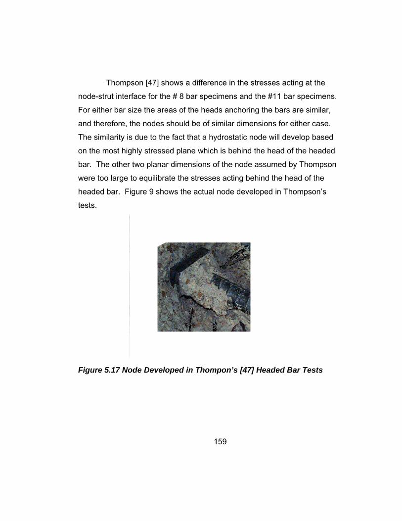
Thompson [47] shows a difference in the stresses acting at the
node-strut interface for the # 8 bar specimens and the #11 bar specimens.
For either bar size the areas of the heads anchoring the bars are similar,
and therefore, the nodes should be of similar dimensions for either case.
The similarity is due to the fact that a hydrostatic node will develop based
on the most highly stressed plane which is behind the head of the headed
bar. The other two planar dimensions of the node assumed by Thompson
were too large to equilibrate the stresses acting behind the head of the
headed bar. Figure 9 shows the actual node developed in Thompson’s
tests.
Figure 5.17 Node Developed in Thompon’s [47] Headed Bar Tests
159
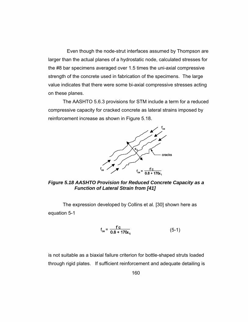
Even though the node-strut interfaces assumed by Thompson are
larger than the actual planes of a hydrostatic node, calculated stresses for
the #8 bar specimens averaged over 1.5 times the uni-axial compressive
strength of the concrete used in fabrication of the specimens. The large
value indicates that there were some bi-axial compressive stresses acting
on these planes.
The AASHTO 5.6.3 provisions for STM include a term for a reduced
compressive capacity for cracked concrete as lateral strains imposed by
reinforcement increase as shown in Figure 5.18.
ε1
fce
fce
cracks
fce = f`c0.8 + 170ε1
ε1
fce
fce
cracks
fce = f`c0.8 + 170ε1
f`c0.8 + 170ε1
Figure 5.18 AASHTO Provision for Reduced Concrete Capacity as a Function of Lateral Strain from [41]
The expression developed by Collins et al. [30] shown here as
equation 5-1
160
fce = f`c0.8 + 170ε1
fce = f`c0.8 + 170ε1
f`c0.8 + 170ε1
(5-1)
is not suitable as a biaxial failure criterion for bottle-shaped struts loaded
through rigid plates. If sufficient reinforcement and adequate detailing is
161
provided that ensures ample plastic deformations, it is unlikely that an
ultimate failure will occur in a cracked region such as the one depicted in
Figure 5.18. Stress redistribution will continue until the stiffest element
has failed in compression at the point of highest stress, which typically
occurs at singular nodes. Collins’ expression (5-1) was developed
through testing of specimens in which the transverse strain was active, in
that, transverse reinforcement within specimens was tensioned while
compressive force was applied. The transverse reinforcement in the
specimens tested in this investigation was strained only through
deformation (passive) of the specimen after a crack through the centerline
had formed and further load was applied. The transverse reinforcement in
some specimens that exhibited the unconfined tensile failure mechanism
was strained well beyond yield, yet the ultimate load was much greater
than that predicted by equation 5-1 indicating that the role of the
reinforcement was only to change the bi-axial stress condition at or around
the nodal area. This point is proven by Figure 5.18 which the efficiency of
concrete to sustain compressive stresses in the presence of transverse
tensile strain normalized to the concrete strength predicted by equation
5-1 is compared with the failure stress of the specimens normalized to the
compressive strength of the concrete of the specimens within the
experimental program.
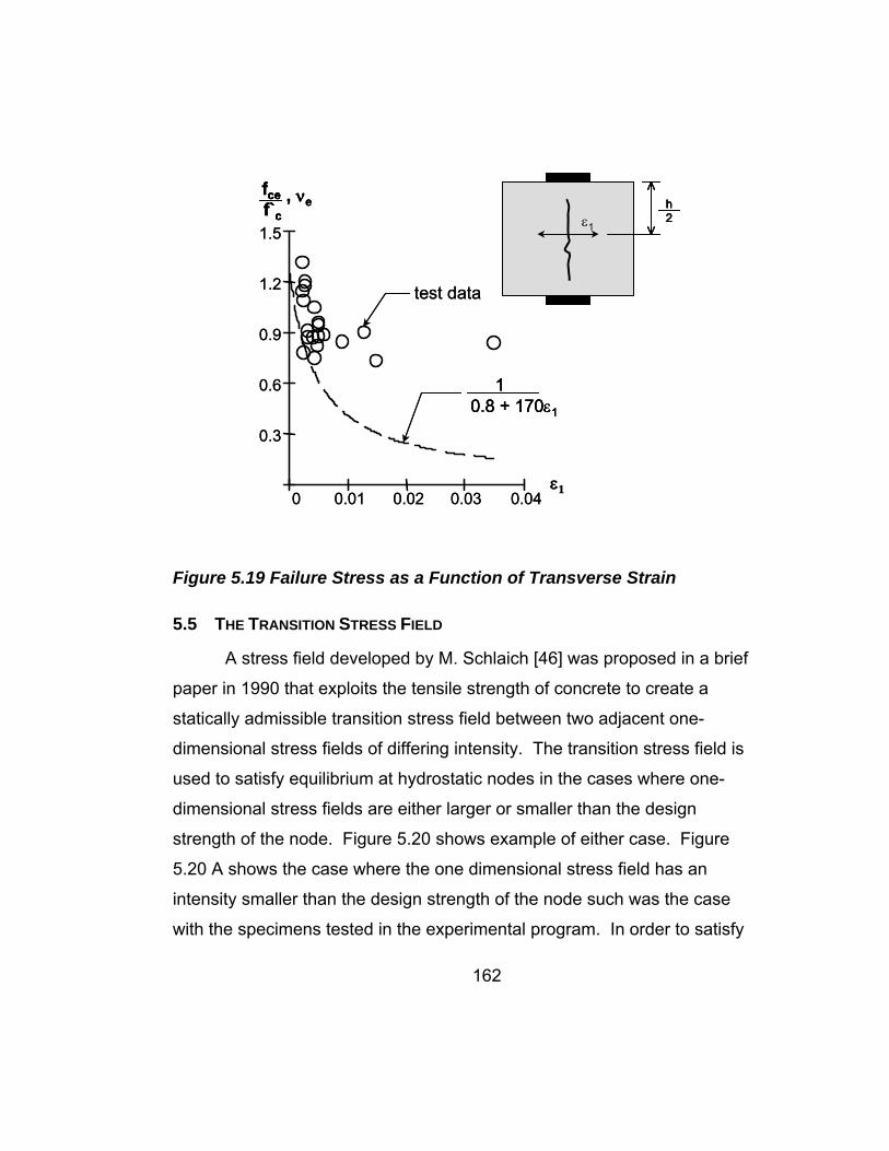
h2ε1
0 0.01 0.02 0.03 0.04
0.3
0.6
0.9
1.2
1.5
_
fce f`c
, νe
10.8 + 170ε1
ε1
test data
h2ε1
h2h2ε1
0 0.01 0.02 0.03 0.04
0.3
0.6
0.9
1.2
1.5
_
fce f`c
, νefce f`c
fce f`c
, νe
10.8 + 170ε1
10.8 + 170ε1
ε1
test data
Figure 5.19 Failure Stress as a Function of Transverse Strain
5.5 THE TRANSITION STRESS FIELD
A stress field developed by M. Schlaich [46] was proposed in a brief
paper in 1990 that exploits the tensile strength of concrete to create a
statically admissible transition stress field between two adjacent one-
dimensional stress fields of differing intensity. The transition stress field is
used to satisfy equilibrium at hydrostatic nodes in the cases where one-
dimensional stress fields are either larger or smaller than the design
strength of the node. Figure 5.20 shows example of either case. Figure
5.20 A shows the case where the one dimensional stress field has an
intensity smaller than the design strength of the node such was the case
with the specimens tested in the experimental program. In order to satisfy
162
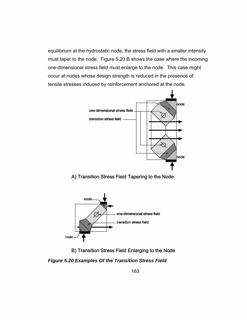
equilibrium at the hydrostatic node, the stress field with a smaller intensity
must taper to the node. Figure 5.20 B shows the case where the incoming
one-dimensional stress field must enlarge to the node. This case might
occur at nodes whose design strength is reduced in the presence of
tensile stresses induced by reinforcement anchored at the node.
transition stress field
one-dimensional stress field
node
node
node
one-dimensional stress field
transition stress field
node
A) Transition Stress Field Tapering to the Node
B) Transition Stress Field Enlarging to the Node
transition stress field
one-dimensional stress field
node
node
transition stress field
one-dimensional stress field
node
node
node
one-dimensional stress field
transition stress field
node
one-dimensional stress field
transition stress field
node
A) Transition Stress Field Tapering to the Node
B) Transition Stress Field Enlarging to the Node Figure 5.20 Examples Of the Transition Stress Field
163
164
The trapezoidal transition stress field is composed of four triangular
stress fields that are in equilibrium with each other and the one-
dimensional stress fields on either end of the transition length.
The trapezoidal stress field separated by each triangular stress field is
shown in Figure 5.21. At the external boundaries of the trapezoid the
normal stresses due to the adjoining one-dimensional stress fields
disappear leaving the stress state inside triangles AOC and BOD one
dimensional and parallel to AC and DB. The tensile force T results in the
one dimensional stress state inside triangles ACO and BDO acting at
angle α with respect to the one-dimensional stresses acting on surfaces
CD and AB. The tensile force T acts across OF while an equal and
opposite compressive force acts across OE. If the intensities of the one-
dimensional stress field are known then the tensile force T depends only
on the length of the transition area dictated by α. To define the length of
the transition area, the compressive stress acting on OE is set equal to the
compressive strength of the concrete defining the position of point O and
the transition length. The tensile strength of concrete can be set at one
value or be reduced according to the intensity of the compressive stresses
present in the one-dimensional stress fields.
Equation 5-2 was derived by M. Schlaich that relates the length of
the transition area in proportion to the initial width of the larger one
dimensional stress field. Equation 5-2 is plotted in Figure 5.22 for various
values of the design strength of the node and a tensile capacity of
concrete equal to 10% of the compressive capacity.

L
A B
O
C DF
νs
νns
Z
E
α
α
β
½ βνns
f'tf'c
1
x
½ Zνs
x = T L Zνs = βνns
T
α
L
A B
O
C DF
νs
νns
Z
E
α
α
β
½ βνns
f'tf'cf'tf'c
1
x
½ Zνs
x = T L Zνs = βνns
T
α
Figure 5.21 Transition Stress Field Adapted from [46]
165

166
ψ12
1f'tf'c
+
f'c
f't
νs
νns⋅ νs νns−⋅⋅
1f'tf'c
+
f'c
f't
νs
νns⋅ νs νns−⋅⋅ψ
12 `` (5-2)
where:where:
ψZL
ψZL
νs
σstrut
f'cνs
σstrut
f'c νns
σnode_strut_interface
f'cνns
σnode_strut_interface
f'c
0 0.1 0.2 0.3 0.4 0.5 0.6 0.7 0.8 0.9 1
0.1
0.2
0.3
0.40.5
0.6
0.7
0.8
0.9
1
ψ
νs
νn/s = 1.0
νn/s = 0.85
νn/s = 0.70
Note:All curves shownwere calculatedwith f`t/f`c = 1/10
strut
strut
strutstrut
strutstrut
strutstrut
0 0.1 0.2 0.3 0.4 0.5 0.6 0.7 0.8 0.9 1
0.1
0.2
0.3
0.40.5
0.6
0.7
0.8
0.9
1
ψ
νs
νn/s = 1.0
νn/s = 0.85
νn/s = 0.70
Note:All curves shownwere calculatedwith f`t/f`c = 1/10
strutstrut
strutstrut
strutstrut
strutstrut
strutstrut
Figure 5.22 ψ-νs Relationship with Differing Values of νns
167
As seen in Figure 5.22 for values of νs less than nodal-strut
compression limit the strut tapers to the node, and for values grater than
the node-strut compression limit, the strut enlarges to the node. The latter
case may apply to nodes anchoring reinforcement in which the biaxial
tension associated with the anchorage of the reinforcement might limit the
compressive stress at the node-strut interface as shown in Figure 5.20 B.
The transition stress field is a planar model as shown in Figure 5.22
that indirectly incorporates a biaxial failure criterion. The planar model
may be improved by adding a stress tensor in the third dimension, but is
beyond the scope of this phase of the research project. The elegancy of
the transition stress field lies in the fact that any biaxial failure criterion can
be implemented. To illustrate this point 3 different biaxial failure criteria
were investigated which are in the form of Kupfer’s [23] envelope for
planar stress.
The first failure criterion was developed using 3 data points
obtained in the experimental program and is shown in Figure 5.23. The
first point (point i) was derived from the average tensile stress and
compressive stress from the split cylinders tested, the second point (point
ii) was computed by integrating the best fit curve of the tensile stress in
the reinforcement (Figure 4.13) just before cracking over the area of
concrete between the nodes and dividing by the mean modular ratio
between all reinforcing steels and concrete used in fabrication of the
specimens. The compressive stress corresponding to this tensile stress
was taken as the average of the best-fit curve of the compressive stresses
at the mid-height of the specimens for each geometrical condition of
loading (Figure 4.22, Figure 4.23). The third point (point iii) was found by
168
averaging the cylinder strengths for all batches of concrete used and was
the value to which all other values were normalized.
The two other bi-axial failure models compared in Figure 5.24 were
the common failure criterion established by Chen and Drucker and given
in the paper by M. Schlaich [46], as well as, a failure criterion that did not
reduce the tensile stress from 0.1 f`c as the intensity of the compressive
stress increased.
In Figure 5.24 6 values of ψ (eq.5-2) as function of the stress in the
strut are plotted. In 3 of the plots a maximum value of 0.85 (νns) for the
node-strut interface was used and in 3 plots the maximum value of 1.0 at
the node-strut interface was used. The discontinuity seen in the curves for
νns equal to 1.0 are the points at which the tensile stress begins to
decrease which, in turn, increase the transition length. The area of the
strut always remains a constant value only dependent on the ratio
between the nodal compression limit and the stress in the strut since the
normal force applied to these two faces are the same. The length of the
transition area depends only on the value of α in Figure 5.21. As the
tensile capacity of the concrete decreases based on the level of
compressive stress applied to the strut face, the length of the transition
area increases based on the value of α which is continually decreasing
toward zero. At an angle of α equal to zero the transition area would no
longer be trapezoidal; it would be square with length of the strut equal to
the length of the node face and equal to the length of the transition area.
This concept is shown in Figure 5.25. As the tensile capacity decreases
at the point of discontinuity the value of ψ as a function of the level stress
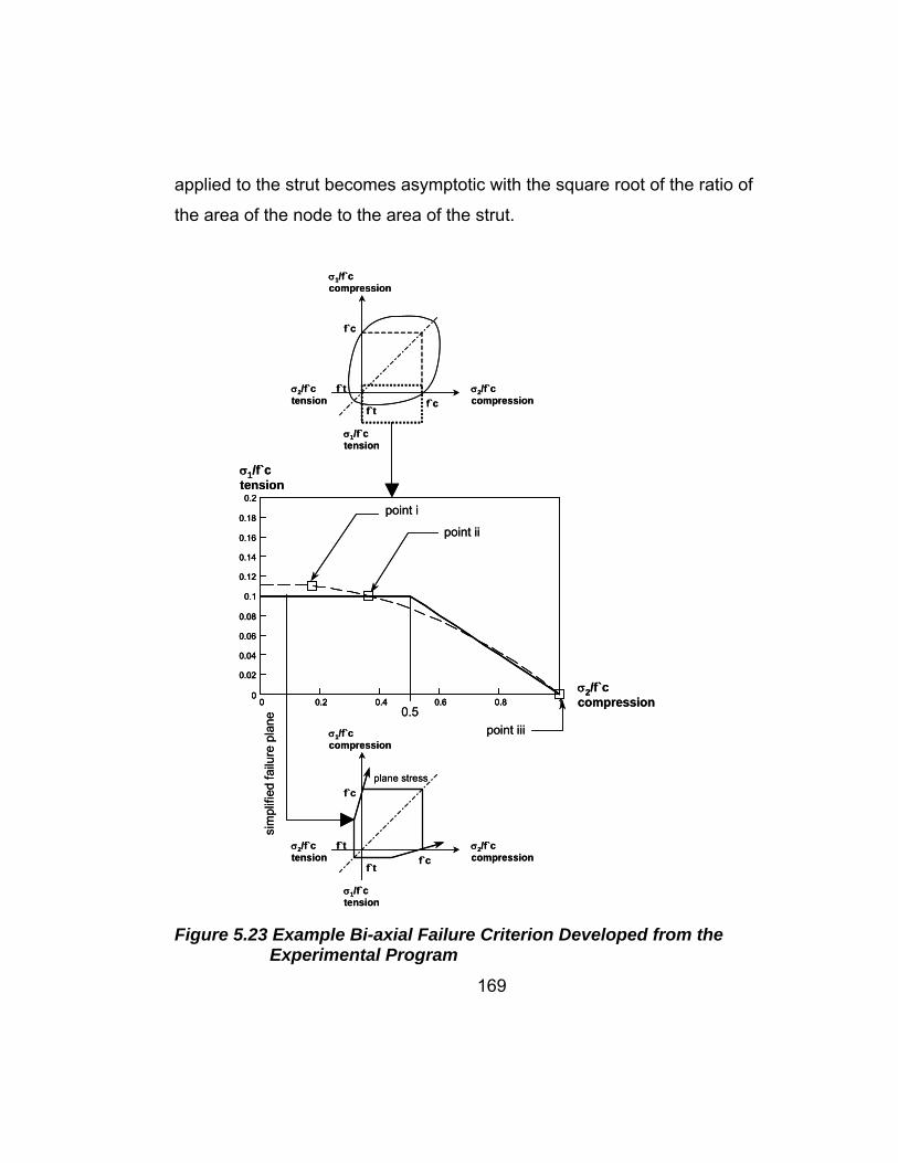
applied to the strut becomes asymptotic with the square root of the ratio of
the area of the node to the area of the strut.
σ2/f`ccompression
σ2/f`ctension
σ1/f`ccompression
σ1/f`ctension
f`c
f`cf`t
f`t
0 0.2 0.4 0.6 0.8 10
0.02
0.04
0.06
0.08
0.1
0.12
0.14
0.16
0.18
0.2point i
point ii
point iii0.5
σ1/f`ctension
σ2/f`ccompression
σ2/f`ccompression
σ2/f`ctension
σ1/f`ccompression
σ1/f`ctension
f`c
f`cf`t
f`t
plane stress
sim
plifi
ed fa
ilure
pla
ne
σ2/f`ccompression
σ2/f`ctension
σ1/f`ccompression
σ1/f`ctension
f`c
f`cf`t
f`t
0 0.2 0.4 0.6 0.8 10
0.02
0.04
0.06
0.08
0.1
0.12
0.14
0.16
0.18
0.2
0 0.2 0.4 0.6 0.8 10
0.02
0.04
0.06
0.08
0.1
0.12
0.14
0.16
0.18
0.2point i
point ii
point iii0.5
σ1/f`ctension
σ2/f`ccompression
σ2/f`ccompression
σ2/f`ctension
σ1/f`ccompression
σ1/f`ctension
f`c
f`cf`t
f`t
plane stress
sim
plifi
ed fa
ilure
pla
ne
Figure 5.23 Example Bi-axial Failure Criterion Developed from the
Experimental Program
169

σ2/f`c
σ1/f`c
f`c
f`cf`t
f`t
5/10
1/10
1/10
5/10
σ2/f`c
σ1/f`c
f`c
f`cf`t
f`t1/15
1/15
11/1511/15
σ2/f`c
σ1/f`c
f`c
f`c
f`t
f`t1/10
1/10
FAILURE CRITERION I FAILURE CRITERION II FAILURE CRITERION III
0 0.1 0.2 0.3 0.4 0.5 0.6 0.7 0.8 0.9 1
0.1
0.2
0.3
0.4
0.5
0.6
0.7
0.8
0.9
1
νs
νns = 0.85
ψ
0 0.1 0.2 0.3 0.4 0.5 0.6 0.7 0.8 0.9 1
0.1
0.2
0.3
0.4
0.5
0.6
0.7
0.8
0.9
1
νs
ψ
νns = 1.0
σ2/f`c
σ1/f`c
f`c
f`cf`t
f`t
5/10
1/10
1/10
5/10
σ2/f`c
σ1/f`c
f`c
f`cf`t
f`t
5/10
1/10
1/10
5/10
σ2/f`c
σ1/f`c
f`c
f`cf`t
f`t1/15
1/15
11/1511/15
σ2/f`c
σ1/f`c
f`c
f`c
f`t
f`t1/10
1/10
FAILURE CRITERION I FAILURE CRITERION II FAILURE CRITERION III
0 0.1 0.2 0.3 0.4 0.5 0.6 0.7 0.8 0.9 1
0.1
0.2
0.3
0.4
0.5
0.6
0.7
0.8
0.9
1
νs0 0.1 0.2 0.3 0.4 0.5 0.6 0.7 0.8 0.9 1
0.1
0.2
0.3
0.4
0.5
0.6
0.7
0.8
0.9
1
0 0.1 0.2 0.3 0.4 0.5 0.6 0.7 0.8 0.9 1
0.1
0.2
0.3
0.4
0.5
0.6
0.7
0.8
0.9
1
νs
νns = 0.85
ψ
0 0.1 0.2 0.3 0.4 0.5 0.6 0.7 0.8 0.9 1
0.1
0.2
0.3
0.4
0.5
0.6
0.7
0.8
0.9
1
νs
ψ
νns = 1.0
0 0.1 0.2 0.3 0.4 0.5 0.6 0.7 0.8 0.9 1
0.1
0.2
0.3
0.4
0.5
0.6
0.7
0.8
0.9
1
νs
ψ
νns = 1.0
170Figure 5.24 Effect of the Failure Criterion on the ψ-νs Relationship
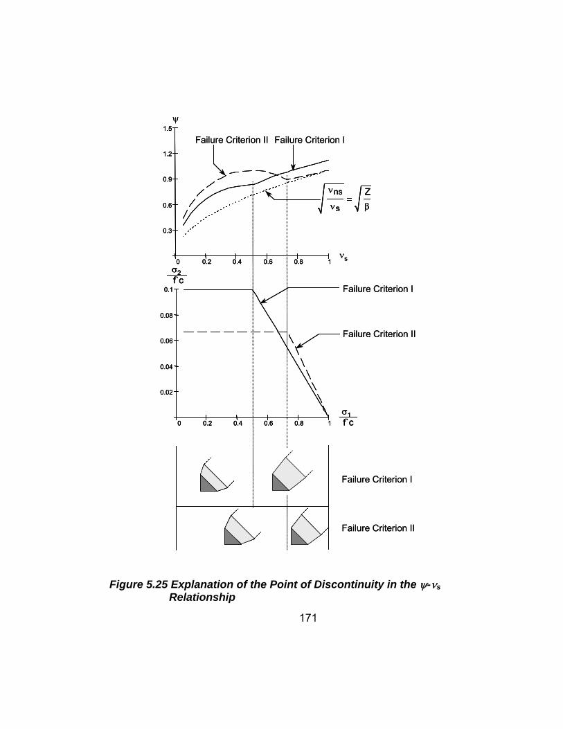
0 0.2 0.4 0.6 0.8 1
0.3
0.6
0.9
1.2
1.5
0 0.2 0.4 0.6 0.8 1
0.02
0.04
0.06
0.08
0.1
Failure Criterion IFailure Criterion II
νns
νs
Zβ
νs
ψ
σ2f`c
σ1f`c
Failure Criterion I
Failure Criterion II
Failure Criterion I
Failure Criterion II
0 0.2 0.4 0.6 0.8 1
0.3
0.6
0.9
1.2
1.5
0 0.2 0.4 0.6 0.8 1
0.3
0.6
0.9
1.2
1.5
0 0.2 0.4 0.6 0.8 1
0.02
0.04
0.06
0.08
0.1
0 0.2 0.4 0.6 0.8 1
0.02
0.04
0.06
0.08
0.1
Failure Criterion IFailure Criterion II
νns
νs
Zβ
νns
νs
Zβ
νs
ψ
σ2f`cσ2f`c
σ1f`cσ1f`c
Failure Criterion I
Failure Criterion II
Failure Criterion I
Failure Criterion II
Figure 5.25 Explanation of the Point of Discontinuity in the ψ-νs Relationship
171

172
5.6 APPLICATION OF THE TRANSITION STRESS FIELD TO TEST DATA
The transition stress field as presented here is a planar model, and
assumes that the stress fields at the node-strut interface and at the strut
face are one-dimensional, as well as the normal force applied to the
transition field is constant. With the fundamental assumptions behind the
model understood, it may reasonably be applied to the specimens tested
in the experimental program only after the basic parameters of the model
are chosen. The two main parameters are the failure criterion used and
the maximum allowable stress at the node-strut interface.
The value of α that determines the length of the transition area is
only dependent on the level of stress applied at the strut face and the
value of ψ which, in turn, is only dependent upon the failure criterion
chosen. The decision made regarding the failure criterion used in the
model was based on the advice of Drucker,
“…once we leave the elastic range, all hope
disappears of finding both a simple and
complete description of the mechanical
behavior. When solving problems simplicity
comes first. Full generality is not the goal; full
generality is complete chaos and contains no
information.”
-Drucker-
and the fact that the observed failure planes were at maximum 10 inches
away from the assumed isosceles triangle forming the singular node. The
simplest failure criterion that results in the shortest transition length was
Failure Criterion III as proven in Figure 5.24. Drucker might consider
173
failure Criterion III full generality; however, when used in combination with
the transition stress field, the information provided by the combination
proves to be valuable.
A correctly chosen value for the node compression limit (νns) poses
some epistemic uncertainty and needs further substation through
experimental testing. It was decided that this value should be set equal to
1.0 indicating the face of the node could withstand compressive stresses
equal to the compressive strength of concrete. The decision was made
based on several planar specimens achieving values of νe greater than 1.0
and as high as 1.3 (S3-4). Since the concrete forming the node was intact
in these specimens, the indication was that the area around the node-strut
interface (area of the transition stress field) could be pushed into the realm
of bi-axial compression if enough reinforcement was provided so that the
value of νns equal to 1.0 was a conservative estimate. It could be argued
that the specimens tested within the experimental program are highly
determinate and therefore were able to achieve such high values of
compressive stress due to the fact that the specimens tested underwent a
constant deformation. For indeterminate structures the failure deformation
is not reached simultaneously for all elements, but at different deformation
stages of the complete system. Therefore, the effective concrete strength
should be reduced according to the theory of plasticity. This point is valid
but depends on the level of stress redistribution in the structure
considered. More experimental testing is needed to prove or refute this
argument. For the time being a value of νns = 1.0 is considered to be
adequate.
174
Once the parameters of the model were chosen, the model could
then be applied to the specimens. The transition stress field, when
applied to one half of the singular node of the specimen is shown in Figure
5.26. The recorded bearing capacity form the specimens tested in the
experimental program can then be applied to the model as the νs value.
Using the bearing capacity as the νs term in the ψ - νs relationship (eq. 5-
20) is justified by the assumptions that the nodes developed at the bearing
plates of the specimens were hydrostatic and the assumption that the
same force was applied to the strut face (area Z in Figure 5.26) and the
node-strut interface (area β in Figure 5.26). Figure 5.27 shows the
transition stress field superimposed on the nodal region of two specimens
tested in the experimental program.

νns, β
νe , Z
L tan (α)
νns β⋅ νe Z⋅
Zνns β⋅
νe
L Z ψ⋅
β 2 Z ψ⋅ tan α( )⋅( )⋅+ Z
α atan1 νe−
2ψ
⎛⎜⎝
⎞⎟⎠
ψ12
1f'tf'c
+
f't
f'c
νe
νns⋅ νns νe−⋅⋅
L
α
where:
Figure 5.26 The Transition Stress Field Applied to the Singular Node of the Specimens
175
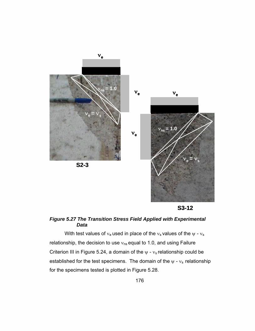
νe
νe = νs
νns = 1.0 νe νe
νeνns = 1.0
νe = νsS2-3
S3-12
νe
νe = νs
νns = 1.0 νe
νe
νe = νs
νns = 1.0 νe νe
νeνns = 1.0
νe = νs
νe
νeνns = 1.0
νe = νsS2-3
S3-12 Figure 5.27 The Transition Stress Field Applied with Experimental
Data With test values of νe used in place of the νs values of the ψ - νs
relationship, the decision to use νns equal to 1.0, and using Failure
Criterion III in Figure 5.24, a domain of the ψ - νs relationship could be
established for the test specimens. The domain of the ψ - νs relationship
for the specimens tested is plotted in Figure 5.28.
176
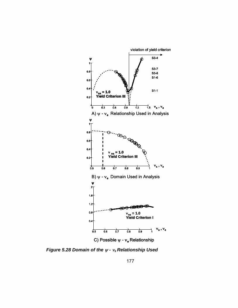
0 0.3 0.6 0.9 1.2 1.5
0.2
0.4
0.6
0.8
1
ψ
νns = 1.0Yield Criterion III
S1-1
S1-6
S3-4
S3-7S3-8
νs , νe
violation of yield criterion
B) ψ - νe Domain Used in Analysis
0.5 0.6 0.7 0.8 0.9 1
0.2
0.4
0.6
0.8
1
νs , νe
ν ns = 1.0Yield Criterion III
ψ
A) ψ - νe Relationship Used in Analysis
0.5 0.6 0.7 0.8 0.9 1
0.4
0.8
1.2
1.6
2
νs , νe
ψ
νns = 1.0Yield Criterion I
C) Possible ψ - νe Relationship
0 0.3 0.6 0.9 1.2 1.5
0.2
0.4
0.6
0.8
1
ψ
νns = 1.0Yield Criterion III
S1-1
S1-6
S3-4
S3-7S3-8
νs , νe
violation of yield criterion
0 0.3 0.6 0.9 1.2 1.5
0.2
0.4
0.6
0.8
1
ψ
νns = 1.0Yield Criterion III
S1-1
S1-6
S3-4
S3-7S3-8
νs , νe0 0.3 0.6 0.9 1.2 1.5
0.2
0.4
0.6
0.8
1
0 0.3 0.6 0.9 1.2 1.5
0.2
0.4
0.6
0.8
1
ψ
νns = 1.0Yield Criterion III
S1-1
S1-6
S3-4
S3-7S3-8
νs , νe
violation of yield criterion
B) ψ - νe Domain Used in Analysis
0.5 0.6 0.7 0.8 0.9 1
0.2
0.4
0.6
0.8
1
νs , νe
ν ns = 1.0Yield Criterion III
ψ
0.5 0.6 0.7 0.8 0.9 1
0.2
0.4
0.6
0.8
1
0.5 0.6 0.7 0.8 0.9 1
0.2
0.4
0.6
0.8
1
0.5 0.6 0.7 0.8 0.9 1
0.2
0.4
0.6
0.8
1
νs , νe
ν ns = 1.0Yield Criterion III
ψ
A) ψ - νe Relationship Used in Analysis
0.5 0.6 0.7 0.8 0.9 1
0.4
0.8
1.2
1.6
2
νs , νe
ψ
νns = 1.0Yield Criterion I
C) Possible ψ - νe Relationship
0.5 0.6 0.7 0.8 0.9 1
0.4
0.8
1.2
1.6
2
νs , νe
ψ
0.5 0.6 0.7 0.8 0.9 1
0.4
0.8
1.2
1.6
2
0.5 0.6 0.7 0.8 0.9 1
0.4
0.8
1.2
1.6
2
νs , νe
ψ
νns = 1.0Yield Criterion I
C) Possible ψ - νe Relationship Figure 5.28 Domain of the ψ - νs Relationship Used
177

178
It can be seen from Figure 5.28 A. that certain test specimens
violated the yield criterion for planar stress meaning that the strut failed at
the node face in a manner conducive to biaxial compression having
compressive capacities in the vicinity of 1.2 f`c. These specimens include
the three specimens tested with 6 in by 6 in bearing plates, and two
specimens fabricated in the first series that were 4 inches thick.
Automatically excluded from this analysis were the two specimens tested
in which the behavior was three dimensional (S3-9, S3-10), and the
specimens in the first series that included confining reinforcement of the
node by means of rectangular ties, which introduce tri-axial compression.
For the specimens not automatically excluded from the analysis, the
violation of the yield criterion possibly resulted in the fact that the area of
steel provided relative to the area of bearing plate was sufficient to confine
the stress field of the strut at the node-strut interface in a bi-axial manner.
Figure 5.28 C is included to remind the reader that any failure criterion
could have been used in this type of analysis. With further testing in
regard to the failure criteria for concrete and maximum compressive
capacities for nodes, a more suitable model might be implemented that
could be easily incorporated into the analysis
The biggest influence on the compressive capacities of the
specimens tested were the amount of transverse reinforcement crossing
the vertical plane perpendicular to the axis at which the load was applied
and the size of bearing plates used to load the specimens. A combination
of these two parameters was plotted that renormalized the percentage of
reinforcement with respect to the area of the bearing plate used to load

the specimens. The plot yielded a straight-line regression shown in Figure
5.29.
As fy⋅ sin γ( )⋅
Ab 63⋅ ksi⋅
_0 0.005 0.01 0.015 0.02
0.4
0.6
0.8
1
1.2
1.4
0.016
νe
λAs fy⋅ sin γ( )⋅
Ab 63⋅ ksi⋅
⎛⎜⎝
⎞⎟⎠
0.74 26.7As fy⋅ sin γ( )⋅
Ab 63 ksi⋅
⎛⎜⎝
⎞⎟⎠
⋅+
_
νeAs fy⋅ sin γ( )⋅
Ab 63⋅ ksi⋅
⎛⎜⎝
⎞⎟⎠
⋅ 1As fy⋅ sin γ( )⋅
Ab 63⋅ ksi⋅0.016≥if
0.6 25As fy⋅ sin γ( )⋅
Ab 63⋅ ksi⋅⋅+
⎛⎜⎝
⎞⎟⎠
otherwise_
As fy⋅ sin γ( )⋅
Ab 63⋅ ksi⋅
_
As fy⋅ sin γ( )⋅
Ab 63⋅ ksi⋅
_
0 0.005 0.01 0.015 0.020.4
0.6
0.8
1
1.2
1.4
0 0.005 0.01 0.015 0.020.4
0.6
0.8
1
1.2
1.4
0.016
νe
λAs fy⋅ sin γ( )⋅
Ab 63⋅ ksi⋅
⎛⎜⎝
⎞⎟⎠
0.74 26.7As fy⋅ sin γ( )⋅
Ab 63 ksi⋅
⎛⎜⎝
⎞⎟⎠
⋅+
_
λAs fy⋅ sin γ( )⋅
Ab 63⋅ ksi⋅
⎛⎜⎝
⎞⎟⎠
0.74 26.7As fy⋅ sin γ( )⋅
Ab 63 ksi⋅
⎛⎜⎝
⎞⎟⎠
⋅+
_
νeAs fy⋅ sin γ( )⋅
Ab 63⋅ ksi⋅
⎛⎜⎝
⎞⎟⎠
⋅ 1As fy⋅ sin γ( )⋅
Ab 63⋅ ksi⋅0.016≥if
0.6 25As fy⋅ sin γ( )⋅
Ab 63⋅ ksi⋅⋅+
⎛⎜⎝
⎞⎟⎠
otherwise_
νeAs fy⋅ sin γ( )⋅
Ab 63⋅ ksi⋅
⎛⎜⎝
⎞⎟⎠
⋅ 1As fy⋅ sin γ( )⋅
Ab 63⋅ ksi⋅0.016≥if
0.6 25As fy⋅ sin γ( )⋅
Ab 63⋅ ksi⋅⋅+
⎛⎜⎝
⎞⎟⎠
otherwise_
Figure 5.29 Linear Regression of the Strut Capacity based on the
Area of Steel Provided Normalized to Area of the Bearing Plate
A reduction from the straight-line regression is also shown that was
fit by passing a straight line through the two lowest values of compressive
capacity based on the amount of steel provided relative to the bearing
179
180
plate dimensions. The reduction of the straight-line regression should
provide conservative estimates of the bearing capacity. The reduction line
was capped where it predicted a compressive capacity of the strut greater
than 1.0 f`c. The cap is needed because the model used to analyze the
specimens is planar with no allowance for bi-axial compression and values
of νe greater than 1.0 violate the yield criterion. Substituting the
conservative equation for the strut capacity based on the reinforcement
provided for the νs term in the ψ - νs relationship with the parameters of νns
= 1.0 and Failure Criterion III in Figure 5.24 produces the curves shown in
Figure 5.30.
As seen from Figure 5.30 as the amount of reinforcement increases
so does the strut capacity until a maximum level of the compressive
strength of the concrete is reached. While the compressive capacity of
the strut face increases to 1.0 the length of the transition area in
proportion of the area of the node face (L/β) decreases to zero and the
area of the strut face (Z/β) relative to the area of the node face decreases
to unity. The inverse of the (Z/β) value is ultimately the effective
compressive force capable of the strut. It can also be seen that the
transition length relative to the length of the node face takes the same
form as the variation of α as a function of the amount of reinforcement
provided. This similarity lies in the fact that the transition length is purely a
function of α which is exclusively a function of the failure criterion chosen.
The maximum capacity of the strut occurs when the transition
length equals zero meaning that the strut face becomes the node-strut
interface. This is consistent with the observations of the confined failure
planes, as well as, the fact that tensile stresses decrease at closer
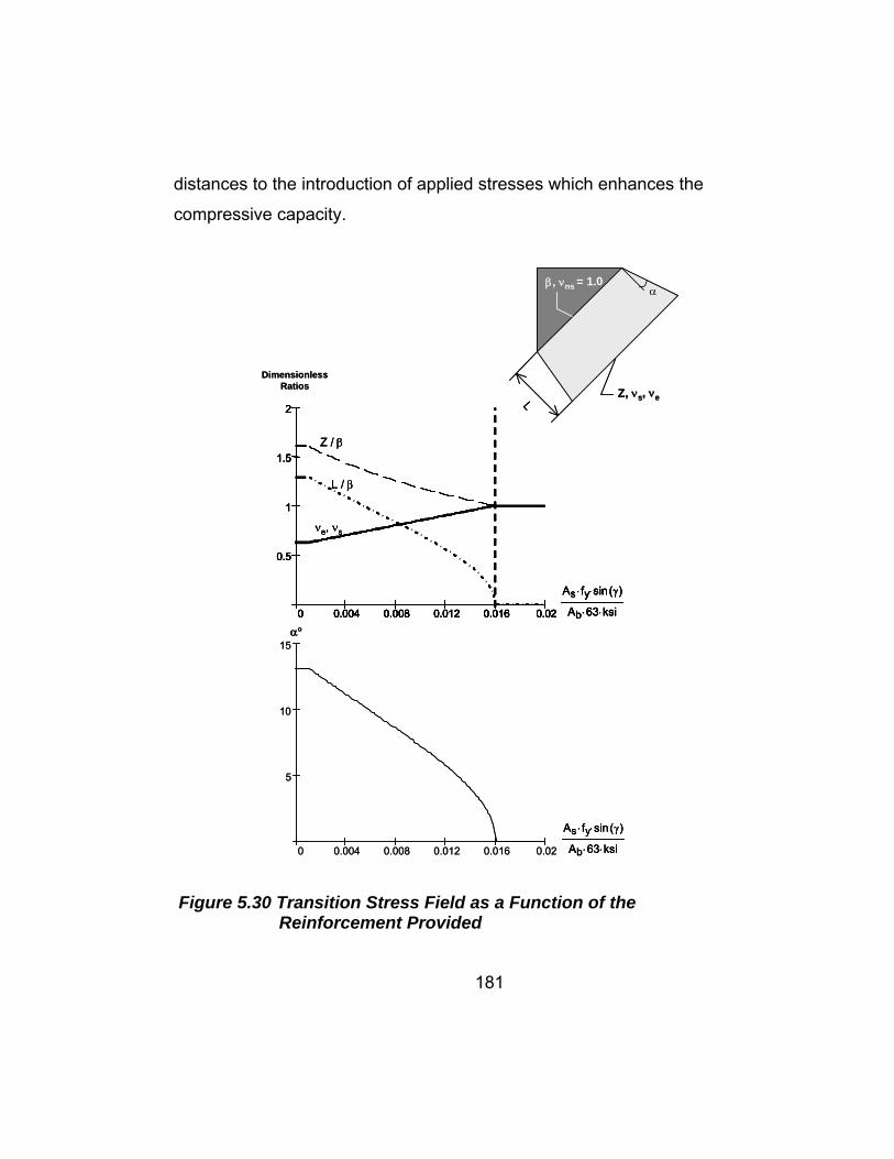
distances to the introduction of applied stresses which enhances the
compressive capacity.
β, νns = 1.0
Z, νs, νeL
α
0 0.004 0.008 0.012 0.016 0.02
0.5
1
1.5
2
0 0.004 0.008 0.012 0.016 0.02
0.5
1
1.5
2
νe, νs
L / β
Z / β
As fy⋅ sin γ( )⋅
Ab 63⋅ ksi⋅
_
0 0.004 0.008 0.012 0.016 0.02
5
10
15
_
As fy⋅ sin γ( )⋅
Ab 63⋅ ksi⋅
_
DimensionlessRatios
α°
β, νns = 1.0
Z, νs, νeL
α
0 0.004 0.008 0.012 0.016 0.02
0.5
1
1.5
2
0 0.004 0.008 0.012 0.016 0.02
0.5
1
1.5
2
νe, νs
L / β
Z / β
As fy⋅ sin γ( )⋅
Ab 63⋅ ksi⋅
_0 0.004 0.008 0.012 0.016 0.02
0.5
1
1.5
2
0 0.004 0.008 0.012 0.016 0.02
0.5
1
1.5
2
νe, νs
L / β
Z / β
As fy⋅ sin γ( )⋅
Ab 63⋅ ksi⋅
_
As fy⋅ sin γ( )⋅
Ab 63⋅ ksi⋅
_
0 0.004 0.008 0.012 0.016 0.02
5
10
15
_
As fy⋅ sin γ( )⋅
Ab 63⋅ ksi⋅
_
As fy⋅ sin γ( )⋅
Ab 63⋅ ksi⋅
_
DimensionlessRatios
α°
Figure 5.30 Transition Stress Field as a Function of the
Reinforcement Provided
181

182
With no reinforcement provided, the maximum capacity of the strut
is equal to 0.6 times the uni-axial compressive strength of concrete
occurring at the maximum distance of 1.3 times the length of the node
face. The maximum compressive force acts over the strut face equal to
1.6 times the length of the node face. If the length of the node face is set
equal to 1.0 then α equals tan-1 ½(1.6-1.0)/1.3 which equals 13 degrees
and is the same value for α depicted in Figure 5.30. The transition stress
field when applied to two specimens within the experimental program in
shown in Figure 5.31. As seen from Figure 5.31, the application of the
transition stress field to both sides of the node leads to developing stress
fields for the entire specimen. From the stress fields the strut-and-tie
model shown in Figure 5.6 B can be envisioned as seen in Figure 5.32.
The ultimate load capable by the strut and hence the specimen is
calculated by dividing the value of β which is always known by Z obtained
from Figure 5.30 based on the amount of reinforcement provided and
multiplying that value by the bearing area of the applied load. This value
shown in Figure 5.31 is a simplification of the ultimate load obtained as
shown in Figure 5.32. Finally, the geometry of the transition stress field
should be checked to ensure that it does not overlap any other stress
fields and is within the boundary of the structural element considered.
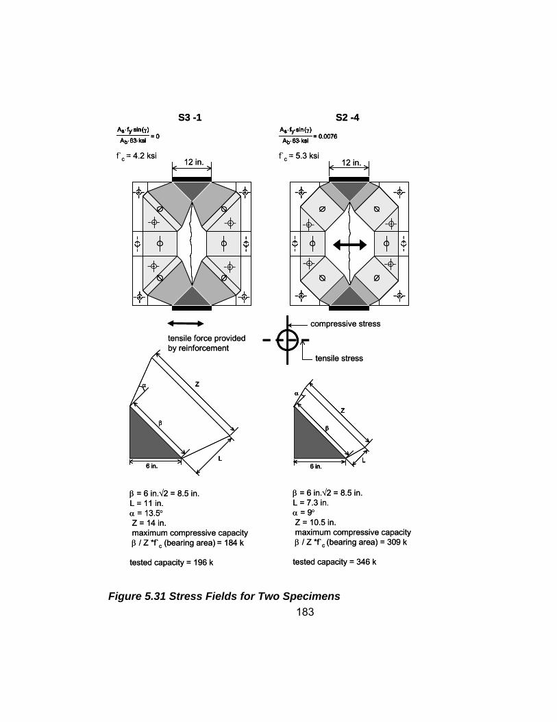
As fy⋅ sin γ( )⋅
Ab 63⋅ ksi⋅
_
= 0As fy⋅ sin γ( )⋅
Ab 63⋅ ksi⋅
_
As fy⋅ sin γ( )⋅
Ab 63⋅ ksi⋅
_
= 0As fy⋅ sin γ( )⋅
Ab 63⋅ ksi⋅
_
= 0.0076As fy⋅ sin γ( )⋅
Ab 63⋅ ksi⋅
_
As fy⋅ sin γ( )⋅
Ab 63⋅ ksi⋅
_
= 0.0076
S3 -1 S2 -4
β = 6 in.√2 = 8.5 in.L = 11 in.α = 13.5°Z = 14 in.maximum compressive capacityβ / Z *f`c (bearing area) = 184 k
tested capacity = 196 k
f`c = 4.2 ksi f`c = 5.3 ksi12 in. 12 in.
β = 6 in.√2 = 8.5 in.L = 7.3 in.α = 9°Z = 10.5 in.maximum compressive capacityβ / Z *f`c (bearing area) = 309 k
tested capacity = 346 k
α
β
Z
L6 in.
α
β
Z
L6 in.
α
β
Z
L6 in.
α
β
Z
L6 in.
tensile stress
compressive stress
tensile force providedby reinforcement
As fy⋅ sin γ( )⋅
Ab 63⋅ ksi⋅
_
= 0As fy⋅ sin γ( )⋅
Ab 63⋅ ksi⋅
_
As fy⋅ sin γ( )⋅
Ab 63⋅ ksi⋅
_
= 0As fy⋅ sin γ( )⋅
Ab 63⋅ ksi⋅
_
= 0.0076As fy⋅ sin γ( )⋅
Ab 63⋅ ksi⋅
_
As fy⋅ sin γ( )⋅
Ab 63⋅ ksi⋅
_
= 0.0076
S3 -1 S2 -4
β = 6 in.√2 = 8.5 in.L = 11 in.α = 13.5°Z = 14 in.maximum compressive capacityβ / Z *f`c (bearing area) = 184 k
tested capacity = 196 k
f`c = 4.2 ksi f`c = 5.3 ksi12 in. 12 in.
β = 6 in.√2 = 8.5 in.L = 7.3 in.α = 9°Z = 10.5 in.maximum compressive capacityβ / Z *f`c (bearing area) = 309 k
tested capacity = 346 k
α
β
Z
L6 in.
α
β
Z
L6 in.
α
β
Z
L6 in.
α
β
Z
L6 in.
tensile stress
compressive stress
tensile force providedby reinforcement
Figure 5.31 Stress Fields for Two Specimens
183

Figure 5.32 Strut-and-Tie Model obtained from the Stress Fields in
Figure 5.31
α
β
Z
L6 in.
α
β
Z
L6 in.
t = 6 in.
β x β x t x f`cZPnode =
Pult = Pnode x 2√2
α
β
Z
L6 in.
α
β
Z
L6 in.
t = 6 in.
β x β x t x f`cZPnode =β x β x t x f`cZβ x β x t x f`cZPnode =
Pult = Pnode x 2√2
Pult = Pnode x 2√2
Figure 5.33 Obtaining the Ultimate load for a Strut from the
Transition Stress Field
184

185
5.7 CONCLUSIONS
The objective of this research project was to either substantiate or
refute the stress limitations for bottle-shaped struts given by ACI 318-02
Appendix A STM provisions and AASHTO LRFD 5.6 STM provisions and
to unify the provisions for bottle-shaped struts given by each code. The
ACI 318-02 Appendix A provisions provided a reinforcement ratio (ACI
equation A-4) as an amount of reinforcement required to confine bottle-
shaped struts to increase their compressive capacity. The substantiation
of this amount of confining steel stipulated by ACI equation A-4 was
necessary to meet the objective
The specimens tested within the experimental program constantly
failed at higher levels of compressive stress than allowed by ACI or
AASHTO. The AAHSTO expression for strut capacity (equation 5-1)
based on active transverse tensile strains in the reinforcement did not
reflect the behavior of the specimens tested, in that, the transverse strains
in the reinforcement were developed passively through deformation of the
specimen and had no detrimental effect on the compressive capacity of
the strut as the strain in the steel increased.
The compressive capacity for bottle-shaped strut as a function of
the amount of steel required to confine the strut is reported here as
equation 5-3 taken from Figure 5.29 without the normalization with respect
to the yield stress of the steel used in the fabrication of specimens.
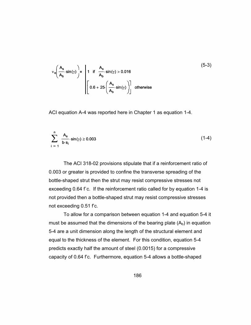
νeAs
Absin γ( )⋅
⎛⎜⎝
⎞⎟⎠
1As
Absin γ( )⋅ 0.016>if
0.6 25As
Absin γ( )⋅
⎛⎜⎝
⎞⎟⎠
⋅+⎡⎢⎣
⎤⎥⎦
otherwise
_
νeAs
Absin γ( )⋅
⎛⎜⎝
⎞⎟⎠
1As
Absin γ( )⋅ 0.016>if
0.6 25As
Absin γ( )⋅
⎛⎜⎝
⎞⎟⎠
⋅+⎡⎢⎣
⎤⎥⎦
otherwise
_
(5-3)
ACI equation A-4 was reported here in Chapter 1 as equation 1-4.
1
n
i
As
b si⋅sin γ( )⋅∑
=
0.003≥
_ 1
n
i
As
b si⋅sin γ( )⋅∑
=
0.003≥
_
(1-4)
The ACI 318-02 provisions stipulate that if a reinforcement ratio of
0.003 or greater is provided to confine the transverse spreading of the
bottle-shaped strut then the strut may resist compressive stresses not
exceeding 0.64 f`c. If the reinforcement ratio called for by equation 1-4 is
not provided then a bottle-shaped strut may resist compressive stresses
not exceeding 0.51 f’c.
To allow for a comparison between equation 1-4 and equation 5-4 it
must be assumed that the dimensions of the bearing plate (Ab) in equation
5-4 are a unit dimension along the length of the structural element and
equal to the thickness of the element. For this condition, equation 5-4
predicts exactly half the amount of steel (0.0015) for a compressive
capacity of 0.64 f’c. Furthermore, equation 5-4 allows a bottle-shaped
186

187
strut to resist compressive stresses equal to the compressive strength of
the concrete if a reinforcement ratio of 0.016 or greater is provided.
M. Schlaich [46] proposed a geometrical stress field that is statically
admissible between two one-dimensional stress fields. This transition
stress field developed by M. Schlaich was used to describe the observed
and recorded behavior of the bottle-shaped struts developed within the
specimens tested. The transition stress field is significant because it
employs a bi-axial failure criterion for concrete under compressive and
tensile stresses, while simultaneously providing a physical geometry for
the stress fields originating from an applied source of loading. The added
information about the geometry of the stress fields helps the designer in
determining sufficient dimensioning of the members of a truss model.
The rudimentary failure criterion used in the stress field developed
by M. Schlaich [46] as it was engaged to the specimens may be altered
with further experimental investigation to incorporate bi-axial compression
and tension in the third dimension or any other combination of stresses in
the three principal axes of a structural element.
With further investigation, the stress field may also be used to
describe the behavior of struts anchored by CCT nodes. Since the
transition stress field depends on allowable values of compressive
stresses placed on various nodes, failure criteria may be developed that
link node and strut behavior for singular nodes. The correlation between
nodes and struts is ideal because the critical stresses within strut-and-tie
models are usually those at the node-strut interface of singular nodes.
References 1. “AASHTO LRFD Bridge Design Specifications, 2nd ed.,” American
Association of State Highway and Transportation Officials, Washington, DC, 1998.
2. ACI 318-02, “Building Code Requirements for Structural Concrete
and Commentary,” American Concrete Institute, Farmington Hills, Michigan, October 2002.
3. ASTM A615/A615M-96a, “Standard Specification for Deformed and
Plain Billet-Steel for Concrete Reinforcement,” American Society for Testing and Materials, West Conshohocken, Pennsylvania, September 1996.
4. ASTM C39/C39M-99, “Standard Test Method for Compressive
Strength of Cylindrical Concrete Specimens,” American Society for Testing and Materials, West Conshohocken, Pennsylvania, September 1999.
5. ASTM C496-96, “Standard Test Method for Splitting Tensile
Strength of Cylindrical Concrete Specimens,” American Society for Testing and Materials, West Conshohocken, Pennsylvania, September 1996.
6. CSA Standard CAN3-A23.3-94, “Design of Concrete Structures for
Buildings with Explanatory Notes,” Canadian Standards Association, Rexdale, Ontario, 1994.
7. “Ontario Highway Bridge Design Code, 3rd Edition,” Canadian
Ministry of Transportation, Toronto, Ontario, Canada, 1991. 8. PCI Design Handbook 3rd Edition, Prestressed Concrete Institute,
Chicago, Illinois, 1985. 9. “Structural Concrete: The Textbook on Behavior, Design, and
Performance - Volume 2: Basis of Design,” Federation Internationale du Beton (FIB), Lausanna, Switzerland, July 1999.
188
10. Adebar, P., Kuchma, D., and Collins, M.P., “Strut-and-Tie Models for the Design of Pile Caps: An Experimental Study,” ACI Structural Journal, Proceedings Vol. 87, No. 1, pg. 81-92, Detroit, Michigan, January-February 1990.
11. Adebar, P. and Zhou, Z., “Bearing Strength of Compressive Struts
Confined by Plain Concrete,” ACI Structural Journal, Proceedings Vol. 90, No. 5, pg. 534-541, Detroit, Michigan, September-October 1993.
12. Adebar, P. and Zhou, Z., “Design of Deep Pile Caps by Strut-and-
Tie Models,” ACI Structural Journal, Proceedings Vol. 93, No. 4, pg. 437-448, Detroit, Michigan, July-August 1996.
13. Ahmed, T., Burley, E., Rigden, S., “Bearing Capacity of Plain and
Reinforced Concrete Loaded over a Limited Area,” ACI Structural Journal, Vol. 95, No. 1, January-February 1998.
14. Ahmed, T., Burley, E., Rigden, S., “Effect of Alkali Silica Reaction
on the Bearing Capacity of Plain and Reinforced Concrete,” ACI Structural Journal, Vol. 96, No. 4, July-August 1999.
15. Bergmeister, K., Breen, J.E., Jirsa, J.O., and Kreger, M.E.,
“Detailing for Structural Concrete,” Center for Transportation Research Report CTR 0-1127-3F, Austin, Texas, May 1993.
16. Breen, J.E., Burdet, O., Roberts, C., Sanders, D., and Wollmann,
G., “Anchorage Zone Reinforcement for Post-Tensioned Concrete Girders,” National Cooperative Highway Research Program Report No. 356, Washington, DC, 1994.
17. Burdet, O, “Analysis and Design of Anchorage Zones in Post-
Tensioned Concrete Bridges,” Ph.D. Dissertation, The University of Texas at Austin, Austin, Texas, August 1990.
18. Chen, B.S., Hagenberger, M.J., and Breen, J.E., “Evaulation of
Strut-and-Tie Modeling Applied to Dapped Beam with Opening,” ACI Structural Journal, Vol. 99, No. 4, July-August 2002.
189

19. Chen, W.F., “Double Punch Test for Tensile Strength of Concrete,” Journal of the American Concrete Institute, Proceedings Vol. 67, No. 12, pg. 993-995, Detroit, Michigan, December 1970.
20. Baumann, Peter, “Die Druckfelder bei der Stahlbetonbemessung
mit Stabwerkmodellen,” Institut fur Massivbau, University of Stuttgart, Germany, 1988.
21. Hawkins, N.M., “The Bearing Strength of Concrete: 1. Loading
Through Rigid Plates Covering Part of the Full Supporting Area,” The University of Sydney, Research Report No. 54, Sydney, Australia, March 1967.
22. Hawkins, N.M., “The Bearing Strength of Concrete: 2. Loading
Through Flexible Plates,” The University of Sydney, Research Report No. 84, Sydney, Australia, August 1967.
23. Kupfer, H., Hilsdorf, H.K., and Rusch, H., “Behavior of Concrete
Under Biaxial Stresses,” Journal of the American Concrete Institute, Proceedings Vol. 66, No. 8, pg. 656-666, Detroit, Michigan, August 1969.
24. Lampert, P. and Thürlimann, B., “Ultimate Strength and Design of
Reinforced Concrete Beams in Torsion and Bending,” IASBE Publications, No. 31-1, pg. 107-131, Zurich, Switzerland, 1971.
25. MacGregor, J.G., “Reinforced Concrete: Mechanics and Design (3rd
Edition),” Prentice Hall, Upper Saddle River, New Jersey, 1997. 26. Marti, P., “Basic Tools in Reinforced Concrete Beam Design,”
Journal of the American Concrete Institute, Proceeding Vol. 82, No. 1, pg. 46-56, Detroit, Michigan, January-February 1985.
27. Marti, P., “Size Effect in Double-Punch Tests on Concrete
Cylinders,” ACI Materials Journal, Proceedings Vol. 86, No. 6, pg. 597-601, Detroit, Michigan, November-December 1989.
28. Marti, P., “Truss Models in Detailing,” Concrete International, Vol. 7,
No. 12, pg. 66-73, Detroit, Michigan, December 1985.
190
29. Maxwell, B.S. and Breen, J.E., “Experimental Evaluation of Strut-and-Tie Model Applied to Deep Beam with Opening,” ACI Structural Journal, Proceedings Vol. 97, No. 1, pg. 142-148, Detroit, Michigan, January-February 2000.
30. Mitchell, D. and Collins, M., “Diagonal Compression Field Theory –
A Rational Model for Structural Concrete in Pure Torsion,” Journal of the American Concrete Institute, Proceedings Vol. 71, No. 8, pg. 396-408, Detroit, Michigan, August 1974.
31. Mörsch, E., “Der Eisenbetonbau, seine Theorie und Anwendung
(Reinforced Concrete, Theory and Application),” Stuggart, Germany, 1902.
32. Mörsch, E., “Über die Berechnung der Gelenkquader,” Beton-und
Eisen, No. 12, pg. 156-161, Stuttgart, Germany, 1924. 33. Muttoni, A., Schwartz, J. and Thürlimann, B.,”Design of Concrete
Structures with Stress Fields,” Birkhaüser, Verlag, Switzerland. 34. Niyogi, S.K., “Bearing Strength of Concrete – Geometric
Variations,” ASCE Journal of Structural Engineering, Vol. 99, No. 7, pgs. 1471-1490, New York, New York, July 1973.
35. Niyogi, S.K., “Concrete Bearing Strength – Support, Mix, Size
Effect,” ASCE Journal of Structural Engineering, Vol. 100, No. 8, pgs. 1685-1702, New York, New York, August 1974.
36. Niyogi, S.K., “Bearing Strength of Reinforced Concrete Blocks,”
ASCE Journal of Structural Engineering, Vol. 101, No. 5, pgs. 1125-1137, New York, New York, May 1975.
37. Ramirez, J. and Breen, J.E., “Proposed Design Procedures for
Shear and Torsion in Reinforced and Prestressed Concrete,” Center for Transportation Research Report No. 248-4F, Austin, Texas, 1983.
38. Reineck, K.H. (Ed), “Examples for the Design of Structural
Concrete with Strut-and-Tie Models,” The American Concrete Institute, SP-208, Farmington Hillls, Michigan, 2002.
191

39. Roberts, C., “Behavior and Design of the Local Anchorage Zone of
Post-Tensioned Concrete Members,” Master’s Thesis, The University of Texas at Austin, Austin, Texas, May 1990.
40. Rogowsky, D.M. and MacGregor, J.M., “Shear Strength of Deep
Reinforced Concrete Continuous Beams,” The University of Alberta, Structural Engineering Report No. 110, Edmonton, Alberta, November 1983.
41. Rogowsky, D.M. and MacGregor, J.M., “Design of Reinforced
Concrete Deep Beams,” Concrete International, Vol. 6, No. 8, pg. 49-58, August 1986.
42. Richart, F., “An Investigation of Web Stresses in Reinforced
Concrete Beams,” University of Illinois Engineering Experiment Station, Bulletin No. 166, Urbana, Illinois, 1927.
43. Ritter, W., “Die Bauweise Hennebique (The Hennebique System),”
Schweizerische Bauzeitung, Bd. XXXIII, No. 7, Zurich, Switzerland, 1899.
44. Sanders, D. “Design and Behavior of Anchorage Zones in Post-
Tensioned Structures,” Ph.D. Dissertation, The University of Texas at Austin, Austin, Texas, August 1990.
45. Schlaich, J., Schäfer, K., and Jennewein, M., “Towards a
Consistent Design of Structural Concrete,” PCI Journal, Vol. 32, No. 3, pg. 74-150, Chicago, Illinois, May-June 1987.
46. Schlaich, M., and Anagnostou, G., “Stress Fields for Nodes of
Strut-and-Tie Models,” Journal of Structural Engineering, Vol. 116, No. 1, pg.13-23, January 1990.
47. Thompson, K. “The Anchorage Behavior of Headed Reinforcement
in CCT Nodes and Lap Slpices,” Ph.D. Dissertation, The University of Texas at Austin, Austin, Texas, May 2002.
192

193
48. Vecchio, F.J. and Collins, M.P., “The Modified Compression Field Theory for Reinforced Concrete Elements Subjected to Shear,” Journal of the American Concrete Institute, Proceedings Vol. 83, No. 2, pg. 219-231, Detroit, Michigan, March-April 1986.
49. Vecchio, F.J. and Collins, M.P., “The Response of Reinforced
Concrete to In-Plane Shear and Normal Stresses,” The University of Toronto, Department of Civil Engineering Publication No. 82-03, Toronto, Canada, 1982.
50. Williams, A., “The Bearing Capacity of Concrete Loaded Over a
Limited Area,” Cement and Concrete Association, Technical Report 526, Wexham Springs, Slough, The United Kingdom, August 1979.
51. Wollman, G. “Anchorage Zones in Post-Tensioned Concrete
Structures,” Ph.D. Dissertation, The University of Texas at Austin, Austin, Texas, May 1992.
52. Young, M.J., “Performance of Headed Reinforcing Bars in CCT
Nodal Regions,” Master’s Thesis, The University of Texas at Austin, Austin, Texas, August 2000.