An experimental study comparing linguistic phylogeneticreconstruction methods

Francois Barbancon,1 Tandy Warnow,1 Steven N. Evans,2 Donald Ringe,3 and Luay Nakhleh4

1Department of Computer Sciences, University of Texas at Austin, Austin, TX 78712, USA2Department of Statistics, University of California at Berkeley, Berkeley CA 94720-3860, USA

3Department of Linguistics, University of Pennsylvania, Philadelphia, PA 19104, USA4Department of Computer Sciences, Rice University, HoustonTX 77005, USA

Abstract

The estimation of linguistic evolution has intrigued many researchers for centuries, and in just the last fewyears, several new methods for constructing phylogenies from languages have been produced and used to analyzea number of language families. These analyses have led to a great deal of excitement, both within the fieldof historical linguistics and in related fields such as archaeology and human genetics. They have also beencontroversial, since the analyses have not always been consistent with each other, and the differences betweendifferent reconstructions have been potentially criticalto the claims made by the different groups. In this paper,we report on a simulation study we performed in order to help resolve this controversy, which compares some ofthe main phylogeny reconstruction methods currently beingused in linguistic cladistics. Our simulated datasetsvaried in the number of contact edges, the degree of homoplasy, the deviation from a lexical clock, and thedeviation from the rates-across-sites assumption. We find the accuracy of the unweighted methods maximumparsimony, neighbor joining, lexico-statistics, and the method of Gray & Atkinson, to be remarkably consistentacross all the model conditions we studied, with maximum parsimony being the best, followed (often closely)by Gray & Atkinson’s method, then neighbor joining, and finally lexico-statistics (UPGMA). The accuracy ofthe two weighted methods (weighted maximum parsimony and weighted maximum compatibility) depends uponthe appropriateness of the weighting scheme, and so dependsupon the homoplasy levels produced by the modelconditions; for low-homoplasy levels, however, the weighted methods generally produce the most accurate resultsof all methods, while the use of inappropriate weighting schemes can make for poorer results than maximumparsimony and Gray & Atkinson’s method under moderate to high homoplasy levels.

1 Introduction

In a phylogenetic analysis, an evolutionary history is proposed for a given set of “taxa”; in biology, the taxa arelikely to be biological species or biomolecular sequences,and in historical linguistics, the taxa are languages, orperhaps dialects, which are presumed to have a common ancestor. In both biological and linguistic phylogeneticanalyses, a set of characters common to all taxa are considered, and each taxon is represented by its states for thesecharacters. A (linguistic) character is any feature of languages that can take one or more forms; these differentforms are called the “states” of the character. Linguistic characters are of three types: lexical, phonological, andmorphological. For lexical characters, the different states are cognate classes, so that two languages exhibit thesame state for the lexical character if and only if they have cognates for the meaning associated with the lexicalcharacter. Phonological characters record the occurrenceof sound changes within the (pre)history of the language;thus a typical phonological character has two states, depending on whether or not the sound change (or, moreoften, constellation of changes) has occurred in the development of each language. Most morphological charactersrepresent inflectional markers; like lexical characters, they are coded by cognation. Thus each character defines

1

an equivalence relation on the language family, such that two languages are equivalent if they exhibit the samestate for the character. Thus, if two languages exhibit the same state for the same character, then the presumptionis (generally) that the shared state arose due to common inheritance. However, shared states can also arise due toborrowing, or through random chance, with some linguistic characters being much more likely to evolve by randomchance or borrowing than others. Thus, not all linguistic characters provide the same quality of “phylogeneticsignal”.

Thus, decisions related to character selection – whether torely only upon lexical characters, or to use mor-phological and phonological characters as well – have the potential to impact a phylogenetic analysis, and thesedecisions also raise other issues, such as whether all characters should be treated identically, or whether “weightingschemes” should be used to reflect the assumed reliability ofthe character. In [30], we examined the impact ofcharacter selection on phylogenetic analyses of an Indo-European (IE) dataset compiled by Ringe and Taylor, andshowed how phylogenetic analyses using the same method can differ when based upon different sets of charac-ters. For example, phylogenies obtained on the basis of lexical characters can be very different from phylogeniesobtained based upon a mixture of the three different types ofcharacters, and phylogenies based upon “screened”datasets (whereby characters are removed if they are considered to be likely to be “homoplastic”) can differ fromphylogenies based upon unscreened datasets. These differences in some cases can be minor, but in other cases canbe significant!

The study in [30] suggests that aspects of character evolution are likely to be significant when evaluatingthe impact of characters on phylogenetic accuracy. For example, a character’s resistance to borrowing could beimportant, since analyzing characters that have evolved through undetected borrowing could lead to an incorrectestimation of the underlying true tree (known in linguistics as the “genetic tree”). However, incorrect phylogeneticreconstructions arise due to a host of reasons. For example,there can be too little evolution in some particularbranch of the true phylogeny for that branch to be correctly reconstructed, resulting typically in an incompletelyresolved tree. There can be “rogue taxa”, which in this case would be languages which have evolved so quicklyfrom their parents that they can attach fairly arbitrarily throughout the tree without changing the quality of theresultant phylogeny; Albanian is an example of this property, to some extent. There can also simply be inadequatedata - just not enough information to resolve the evolutionary history. The degree of deviation from a lexical clockcan negatively impact methods, as can the degree of homoplasy (parallel evolution or back-mutation).

All of these issues have the potential to impact all phylogenetic reconstruction methods, and yet it is clear thatdifferent methods respond differently to these challenges, with some methods more negatively impacted by someconditions than others.

How, therefore, is an interested researcher to determine whether a particular phylogenetic analysis proposedfor a given language family is reliable? Or to determine whatphylogenetic reconstruction method to use whengiven a particular character dataset? Or to determine whichcharacters to use in a new phylogenetic analysis? Orto understand why two phylogenetic analyses might differ? Explicit models of language evolution – especiallyparametric ones – will greatly enable the exploration of howdifferent conditions impact the accuracy of differentphylogeny reconstruction methods, and help us answer thesequestions.

Models of linguistic character evolution Various stochastic models of linguistic character evolution have beenproposed or implicitly suggested in simulation studies andstatistical analyses of language evolution [14, 22, 25,1, 31]. Models of linguistic character evolution differ in several ways: (a) they may assume that all evolution istreelike, so that no borrowing occurs, or they may explicitly model borrowing, (b) they may assume that evolution isclock-like or not, (c) they may assume that characters evolve identically or not, (d) they may assume that differentcharacters evolve independently, or not, and (e) they may allow homoplasy to occur, or not. For example, in[25] we proposed the “perfect phylogenetic network” non-parametric model of language evolution in which everycharacter evolves down a tree contained within a network, but without any homoplasy, and in [39] we proposed aparametric model that allows for borrowing and limited homoplasy.

Parametric stochastic models are those in which the probability distribution of the observed data comes froma given family of possible distributions, with the actual member of the family being determined by a collection of

2

numerical parameters. For example, a parametric model may assume that all characters evolve independently, butwithout any homoplasy, and require extra parameters to specify the probability that a given character will changeits state (and thus evolve into a new state) on a given edge in the tree. Thus, the model is fully specified by theunderlying tree and the parameter values for the substitution mechanism. One of the virtues of a parametric modelis that simulation studies can be performed under the model,which allows a researcher to study the accuracy ofa reconstruction method under a range of conditions. That is, in a simulation study, the researcher selects (orrandomly generates) a model phylogeny, which may either be atree or a network (a tree with contact edges, whichare added to model borrowing). Characters are then evolved down the phylogeny, thus producing states for eachcharacter at every leaf in the phylogeny. This resultant character state matrix (where the rows correspond to thelanguages that occupy the leaves of the phylogeny, and the columns correspond to the characters) can then be givento a collection of phylogeny reconstruction methods. The resultant phylogenies are computed, of course, withoutknowledge of the model phylogeny, and hence may have errors.However, these estimated phylogenies can eachbe compared to the model phylogeny, and the degree of error can be quantified. By performing simulation studies,it is possible to determine various aspects of the performance of phylogeny reconstruction methods. For example,it is then possible to characterize the model conditions (i.e., parameter values) under which a method will yielda highly accurate estimation, and those under which the method will be more likely to have errors. It can alsobe possible to characterize the model conditions under which all methods do well, or all methods do poorly, or -perhaps - one method outperforms another.

To our knowledge, the most complex model of language evolution is the one we provided in [39], whichallows characters to evolve with limited (but identifiable)homoplasy, borrowing between lineages, and assumesthe characters evolve independently but not identically. Under this complex model, we showed in [39] that withlimited borrowing, the evolutionary history is identifiable (which implies that given enough data, the true historycan be reconstructed if a good reconstruction method is used), and we provided polynomial time algorithms whichare statistically consistent under the model. However, these theoretical results do not provide any direct insight intothe relative performance of any methods on finite datasets (as identifiability and statistical consistency are conceptsthat address what is possible given unbounded amounts of data).

Simulation studies have been used to evaluate the performance of phylogeny reconstruction methods in molec-ular systematics (i.e., the estimation of phylogenies fromDNA, RNA, or amino-acid sequences), and have beenable to shed light on how different molecular evolutionary processes impact phylogenetic accuracy. For example,such simulation studies have been used to show how rates of evolution, taxonomic sampling, reticulation events,and deviations from a molecular clock (the biological equivalent of a lexical clock, which asserts that the numberof times each site within a molecular sequence changes should be proportional to time) impact absolute accuracyas well as the relative performance of different phylogenetic reconstruction methods (the scientific literature is toolarge to provide a comprehensive list of papers, but see [6, 15, 19, 24, 26, 27, 28]). These studies tend to lendsupport to the conjecture that statistical estimation methods, such as maximum likelihood, will produce the mostaccurate results, provided that the statistical estimation methods are based upon models that are a good fit to theunderlying evolutionary processes (which, of course, cannot be known on a real dataset).

Linguistic evolution has many of the same features as biological sequence evolution, but certain issues areof particular relevance because of differences between thetwo domains. In particular, in linguistic evolution (ascompared to biological sequence evolution), there is generally much less homoplasy. That is, in our experience,careful application of the Comparative Method [16] by an experienced and knowledgeable historical linguist canidentify many of the borrowings between languages, and thusproduce data matrices which have very little ho-moplasy. In addition, since certain characters are known toevolve through parallel evolution, these can also beidentified in advance, and screened out (removed from the analysis). Finally, some phylogenetic reconstructionsof language families have been based solely upon lexical data, while others have used morphological and complexphonological characters as well.

In this paper we provide a simulation study in order to address how different features of evolutionary processesimpact the accuracy of phylogenies estimated from linguistic character data, using phylogeny reconstruction meth-ods that have been used in recent analyses of linguistic datasets. We describe the experimental design in Section

3

2, and report on the results of this experiment in Section 3. We then conclude in Section 4 with a discussion aboutongoing work in modelling language evolution.

2 The simulation study

2.1 Overview

We performed a simulation study under the model we provided in [39], in order to evaluate the performance of sixexisting phylogeny reconstruction methods under a wide range of model conditions. All model networks and treeswe used had 30 leaves, and ranged from no contact edges (i.e.,tree-like evolution) to networks with three contactedges. To capture the characteristics of a real dataset, such as the IE dataset that was analyzed in [30], we evolvedfrom 301 to 361 characters down the trees, the bulk of which (300 or more) were modelled after lexical characters,and the remainder were morphological. We set the parametersof the simulation in order to produce datasets withdifferent homoplasy levels, deviations from a lexical clock, and deviations from the rates-across-sites assumption.

We had two types of characters, lexical and morphological, and we divided lexical characters into three typesaccording to the rate of evolution, obtaining fast lexical,medium lexical, and slow lexical characters. Within eachof the four types of characters, the parameters of the evolutionary process were drawn identically and independentlyfrom a distribution which we describe below.

Our experiment was designed to help us understand how the conditions of the evolutionary process (e.g.,the presence of borrowing between lineages (i.e., reticulations), relaxing the strong molecular clock, relaxingthe rates-across-sites assumption, and the degree of homoplasy) impact the accuracy of the different phylogenyreconstruction methods we studied. However, we were also interested in seeing if there were any clear indicationsof relative performance between different methods, in evaluating the consequences for “screening datasets” toremove likely homoplastic characters, in using weighting schemes to give higher weight to those characters whichwere considered likely to be more resistant to homoplasy, and in restricting analyses to lexical-only datasets ascompared to using lexical and morphological characters together.

2.2 Phylogeny reconstruction methods

The phylogeny reconstruction methods we study in this paperinclude most of the standard methods used in molec-ular phylogenetics as well as two newer methods proposed explicitly for reconstructing phylogenies on languages.The methods studied include four character-based methods and two distance-based methods. The four character-based methods each produce several trees, and hence we use a standard consensus method (the “majority con-sensus”) in order to return a single estimate of the evolutionary history. (See [11, 38] for two books providinginformation on phylogenetic reconstruction methods used in biology, including many of the methods studied here.)

UPGMA The UPGMA (unweighted pair grouping method of agglomeration) algorithm is a distance-based methodwhich is designed to work well when the evolutionary processes obeys thelexical clockassumption. This is thesame method used in lexicostatistical analyses. As is standard for this method, we use Hamming distances (thenumber of characters on which a given pair of languages have different states) to define the distance matrix betweenthe set of languages.

Neighbor joining NJ, orNeighbor Joining[34], is a particular agglomerative clustering technique used in molec-ular phylogenetics, which is able to reconstruct accurate phylogenies even when the clock assumption does nothold. Of all distance-based methods, NJ is believed to be oneof the best. The corrected distanceD(i, j) betweentwo languagesi andj is computed by calculating corrected distances for each type of character (i.e., slow lexical(SL), medium lexical (ML), fast lexical (FL) and morphological (Mo)), and then averaging them:

D(i, j) =numSLDSL(i, j) + numMLDML(i, j) + numFLDFL(i, j) + numMoDMo(i, j)

numSL + numML + numFL + numMo

4

wherenumX is the number of characters in classX asX ranges over the four classes of characters,HDX(i, j)is the Hamming Distance between languagesi andj computed only on the basis of the characters in the classX , andDX(i, j) = − log(1 − HDX(i, j)/numX). Under the model we propose, if we do not allow reticulation,homoplasy or heterotachy (that is, violation of the rates-across-sites assumption), then theD(i, j) will be consistentstatistical estimators of genuine tree distances that are concordant with the topology of the underlying genetictree. That is, when the numbers of replicatesnumX are large, theD(i, j) will be close to a collection of leaf-to-leaf distances on a tree with edge lengths whose shape is that of the genetic tree. (Note that using NJ withuncorrected distances is not a statistically consistent estimator of phylogenies, except for cases where the lexical-clock assumption holds.)

Maximum parsimony and weighted maximum parsimony Maximum Parsimony, or MP, is an optimizationproblem which seeks a tree on which a minimum number of character state changes occurs. When the charactersare weighted, then the objective is to find a tree in which the total weighted number of character state changes isminimized. Both MP and WMP are NP-hard problems, which has the consequence that exact solutions cannot beguaranteed using polynomial time algorithms. Hence, we useheuristics in the PAUP* [37] software package tofind good (though not provably optimal) solutions. Since there can be many equally good solutions, the majorityconsensus tree of the set of optimal solutions is returned. In our experiments, we used a weighting scheme wherethe weight of every morphological character is 50, and the weight of every lexical character is 1; this weightingscheme was selected on the basis of the perceived relative resistance of thescreeneddatasets we analyzed in [30],and so reflects the expectation that screened morphologicalcharacters will be much more resistant to homoplasyand borrowing than screened lexical characters.

Weighted maximum compatibility When all the characters evolve without homoplasy down a tree, then thetree is called a “perfect phylogeny”, and each of the characters is said to be “compatible” on the tree. WeightedMaximum Compatibility, or WMC, is the optimization problemwhich seeks a tree with the maximum weightedcompatibility score, which is computed by adding up all the weights of each character which is compatible onthe tree. WMC is an NP-hard problem, which we “solve” heuristically through the use of the WMP (weightedmaximum parsimony) analysis – by taking all the trees which are optimal for WMP, scoring each one under theWMC criterion, and then returning those trees which are optimal under WMC. Once again, we return the majorityconsensus of the best trees we find. Since WMC (like MP and WMP)is NP-hard, these solutions are not guaranteedto be globally optimal solutions.

Gray & Atkinson’s method (G&A) The method (originally presented in [14]) designed by Russell Gray andQuentin Atkinson operates as follows. First, each multistate character is replaced by a binary encoded version ofthe character, and these binary characters are then interpreted as restriction sites and analyzed under a rates-across-sites model in the MrBayes software [20]. MrBayes uses a Markov chain Monte Carlo exploration of tree andparameter space to simulate the Bayesian posterior distribution of the tree and parameters under its model. The runof the Markov chain is divided into aburn-inand astationaryphase of equal length. Each phase contains 75,000iterations. During the second,stationaryphase, 100 simulated values are recorded at regular intervals. We reportthe majority consensus tree of those 100 values.

Comments These six methods are most of the ones that have been used in phylogenetic reconstructions onlinguistic datasets: UPGMA is the standard method used in lexico-statistics, maximum parsimony has been used inseveral dataset analyses (see for example the analysis of the Bantu language family in [17]), and Gray & Atkinsonused their method to analyze an Indo-European dataset [14] and to analyze the Bantu language family [18]. Inour own analyses [25, 30, 32] of IE datasets, we have used methods designed to find trees that optimize weightedmaximum compatibility; most recently, we have modified thisapproach by looking for “perfect phylogeneticnetworks” which use the obtained trees as candidates for theunderlying genetic tree. Thus, WMC is included inorder to represent a technique that is closely allied to our approaches. Neighbor joining is included in order to

5

provide a method from the biological systematics toolkit (although it has also been used in phylogenetic analysesfor language families).

Some comments should be made about the use of weighting in maximum parsimony or maximum compati-bility. The weights in these methods are supposed to reflect the relative resistance to borrowing and homoplasy,with higher weights given to characters that are believed tobe more resistant to borrowing and homoplasy. Inour studies, we have used WMConly afterthe data have been screened to remove clearly homoplastic characters.In our simulation study, we have the weights for all lexical characters set to 1 and weights for all morphologicalcharacters set to 50, to reflect the expectation that morphological characters, after screening, will have a very lowincidence of homoplasy and borrowing, as compared to lexical characters. Thus, WMC and WMP shouldnot beused in this way on unscreened data. However, we include datashowing how WMC and WMP perform on un-screened data in order to show how the use of extremely poor estimates of character weights impacts phylogeneticaccuracy.

Software We used PAUP* [37] for all the phylogeny reconstruction methods we studied, except for Gray &Atkinson. For our implementation of Gray & Atkinson, we usedMrBayes [20]. We used the r8s program [35] togenerate our model trees. See the appendix for the commands we used.

2.3 Model network generation

Our simulation generates random binary trees using a Yule process with per individual birth rate1 conditioned tohave the requisite number of terminal taxa at time1, as implemented by Sanderson’sr8s software [35]. Thus, thetrees we generated by r8s have edge lengths that represent elapsed time, and are normalized so that all paths fromroot to terminal leaf have length1. We indicate the elapsed time on edgee by t(e).

In our model of evolution, the implementation of borrowing requires the existence of contact edges betweenlineages. Those contact edges must be added to the generatedbinary tree and the resulting structure is no longer atree but a network. Two languages must be in existence at the same absolute time to borrow from each other. Thuscontact edges can only be generated between points that are equidistant from the root.

Suppose we have a pair of tree edges in different lineages that overlap for some interval of time[t1, t2]. Lett0 ≤ t1 be the time of the most recent common ancestor of the points inthe two edges. We begin by layingdowncandidatecontact edges according to an inhomogeneous Poisson process – some of these candidate contactedges will be removed to form the final reticulate network viaa procedure that we describe below. The infinitesimalprobability that a candidate contact edge occurs during thetime interval[t, t+dt] between the two edges is initiallyµ(t− t0)

−1 dt for t1 ≤ t ≤ t2, whereµ is some parameter controlling the initial laying down of candidate contactedges. This prescription has the two features that the probability a pair of edges will be connected by a contactedge is increasing with the length of the overlap of the edgesin time and decreasing from the time at which thelineages containing the edges diverged.

The inclusion of contact edges between two edges that issue from the same branch point doesn’t introducereticulation and so we discard such candidate edges. We would then like to condition the contact edge generationprocess to create exactlyn contact edges (for some specified integern) between edges that don’t issue from thesame branch point. This conditioning eliminates the parameterµ and gives a network with a prescribed number ofpossibilities for borrowing. We may approximate the effectof such a conditioning by the following procedure thatallows at most one contact edge between any two tree edges.

• For each pairπ of tree edges that overlap for some non-empty time interval[t1, t2] and have their most recentcommon ancestor at timet0 < t1 (so that the edges don’t issue from the same branch point), assign a scoreS(π) given by

S(π) = − log(t1 − t0)

(t2 − t0).

6

• Draw without replacementn pairs of edges, such that each pairπ is drawn with probability equal to itsnormalized scoreS(π)/

∑

π′ S(π′).

• Oncen such edge pairs have been drawn, the corresponding contact edges are drawn by generating a timeof contacttc for the edge via

tc = t0 + (t1 − t0) exp

(

U log((t2 − t0)

(t1 − t0))

)

,

whereU is a random variable uniformly distributed on[0, 1] and these random variables are independent fordifferent edge pairs. In particular, each pair of edges in the tree is connected by at most one contact edge.

2.4 Stochastic model of language evolution

We use the stochastic model of language evolution proposed in [39]. In that model, there is a fixed collection oflinguistic characters, each of which has an infinite collection of possible states. A language is represented by theparticular states it exhibits for each of the characters (note, however, that two leaves in the treemaybe identicalwith respect to the characters, due to insufficient evolution). Languages evolve down an underlying tree with addedreticulate edges that represent contact events between lineages. At a contact event, the state of each character maybe instantaneously transferred from the lineage at one end of the edge to the lineage at the other end (that is, onelineage “borrows” the character state of another), and replaces the character state inherited from its genetic parent.

The set of possible states for a given character consists of adistinguished stateh∗, which we call the homo-plastic state, that may arise at several points in time in thesame or different lineages, and an inexhaustible set ofstates denotedn, n′, n′′, . . ., which we call the non-homoplastic states, each of which mayarise no more than onceacross all times and all lineages as the result of a transition from another (homoplastic or non-homoplastic) state.

Given an edge in a model tree with edge lengthst(e) indicating elapsed time on the edgee, the transition eventsalong the edge follow a homogeneous Poisson process with a rate to be described later.

In this paper we simplify the model of single character evolution by taking the transition probabilities to beidentical for all edges and all characters and to depend on a single parameter0 ≤ homoplasy factor(c) ≤ 1 whichdepends upon the characterc, as follows:

• Pr(h∗, h∗) = Pr(n, n) = 0

• Pr(n, h∗) = homoplasy factor(c)

• Pr(n, n′) = 1 − homoplasy factor(c)

• Pr(h∗, n) = 1

The probability that the state of a characterc is transferred along a contact edgee depends upon two parame-ters, one which depends upon the edge, and one which depends on the character. The parameter that depends uponthe edge isedge borrowing(e), which is the probability that the most easily borrowed character transmits a statein one of the two directions for the edge. This parameter can depend upon the edge, to reflect the possibility thatsome contact events are more extensive than others; however, in our simulation study we setedge borrowing(e)to the same value for all edges. The other parameter ischaracter borrowing(c), which reflects the probabilitythat the character will transmit its state across a contact edge. This parameter depends upon the character sincesome character types are more easily borrowed than others (in particular, some lexical characters and morpholog-ical characters are not readily borrowed, but other lexicalcharacters and some phonological characters are easilyborrowed). In our simulations, we setcharacter borrowing(c) for each of the different character classes, but set itto 0 for the morphological characters since we do not permit themto be borrowed. For a given edge and character,the probability of borrowing in one direction along the edgeis the same as the probability of borrowing in theother direction. Thus, the probability of characterc transmitting its state in one direction on the edgee is given by1

2edge borrowing(e) × character borrowing(c).

7

2.5 Character evolution

The phylogenetic network consists of an underlying genetictree with additional contact edges, whose edge lengthst(e) represent the elapsed time on edgee (so that contact edges havet(e) = 0). We now describe additionalparameters so that we can describe how each character evolves down this network, independently of the othercharacters.

We begin by defining the expected number of changes of a given character on a given edge. This expectednumber of changes will depend upon the edgee (and specifically ont(e)), but also on some additional parame-ters which we need to define. However, before we define these parameters we need to describe the concepts ofultrametricityandrates-across-sites.

The condition of ultrametricity is that the path length fromthe root to each leaf is identical; when all taxa arecurrent-day and path lengths represent time, ultrametricity is immediate. However, when path lengths representthe expected number of changes of a random site, then ultrametricity depends upon thelexical clockhypothesis,which is generally discounted. We quantify the deviation from the lexical clock through the use of a parameterσ0

which we define below.The rates-across-sites assumption is quite standard in molecular systematics and its underlying models, but is

nevertheless also questionable. It states that every two characters evolve proportionally – so that if one characterevolves at twice the speed of another character on one branchof the tree, then it evolves at twice the speed of theother character on every branch in the tree. We quantify the deviation from this assumption through the parameterσ1, which we also define below. (See [10] for a study discussing the rates-across-sites assumption and statisticalidentifiability of divergence times.)

We now define the expected number of transitions on edgee for characterc to be:

t(e) × Ve × height factor(c) × Wc,e,

whereheight factor(c) is a parameter that only depends on the class of the characterc, andVe andWc,e arerandom variables with

Ve = exp(Xe − σ2

0/2), Xe ∼ N(0, σ2

0)

andWc,e = exp(Xc,e − σ2

1/2), Yc,e ∼ N(0, σ2

1).

The normal random variablesXe andYc,e are independent over all choices of edgee and characterc. Note thatVe

andWc,e both have mean1. The parameterσ0 controls the degree to which the model deviates from a lexical clock(that is, fails to be ultrametric). The parameterσ1 controls the degree to which therates-across-sitesassumptionfails.

Model conditions Certain parameters of the model are specific to the phylogenetic network but vary with the ex-periments; these include the model phylogeny topology (in particular the number of contact edges) and the elapsedtime on each edge. We fix the parameteredge borrowing(e) which indicates the probability of a character state be-ing transmitted on the edge. In addition to these network-specific parameters, there are parameters that can changeaccording to the character; these includehomoplasy factor(c), character borrowing(c), height factor(c), devi-ation from lexical clock(represented by the parameterσ0), andheterotachy(represented by the parameterσ1).

We add the following constraints to the parameter system to suppress additional degrees of freedom unneces-sary for the purpose of our experiments:

• We set the parametersσ0 andσ1 identically for all characters within any one simulation, but vary theseparameters between different experiments.

• The other parameters have one set value for each of the four character classes we consider.

• The value ofheight factor(c) only depends on the class of the character and increases as wego from slow tomedium to fast lexical characters. Its value for morphological characters is the same as that for slow lexicalcharacters.

8

• The values ofhomoplasy factor(c) andcharacter borrowing(c) are identical across the three classes ofslow, medium and fast lexical characters. They only differ between lexical and morphological characters.

• Because morphological characters will not undergo borrowing,character borrowing(c) is a parameter forlexical characters only. We are therefore able to add the constraint that for all contact edges and for all char-acter classesedge borrowing(e) = character borrowing(c), which reduces the parameterization related toborrowing to a single parameter.

For each experiment, we set the above stochastic parameterspartly by targeting measurable model conditionssuch as observed homoplasy and borrowing, as well as other considerations such as the number of contact edges,number and type of characters analyzed, etc. For each experiment, we generate32 random networks by taking atree generated by r8s and adding the contact edges. For each of these networks, we make three random draws ofthe random variables (Ve andWc,e). For each of these draws, we generate three random sequences of charactersat the root and simulate their evolution. In total, for each each experiment, we generate a data point averaged over288 measurements:32 topological networks×3 draws of the random variables×3 randomly evolved datasets.

The state at the root of each character is drawn ash∗ (with probability homoplasy factor(c)) or n (withprobability 1-homoplasy factor(c)). After each run of the simulation process, we obtain a set ofsequences,one for each leaf in the phylogenetic tree or network, where each sequence represents the states of the languagerepresented by that leaf for each of the characters in the simulation process. This resulting character state matrixis used by each reconstruction method to produce an estimated tree, which can then be compared with the genetictree within the model phylogenetic network.

Preliminary experiments showed that most of the variability in the estimated trees was due to variability in thenetwork, and this is why we have many more replicates of the network itself, rather than evolving many datasetsdown any given network.

2.6 Error rates for phylogeny reconstruction methods

We compute two types of error rates: “false negatives” and “false positives”, which we now define. Recall that eachphylogeny reconstruction method produces a tree, which is compared to the “genetic tree” contained within themodel network. (That is, although a phylogenetic network can contain many trees, there is an underlying binarytree to which the contact edges are added in order to produce the network; it is this tree that we will make ourcomparisons to.)

Every edge in a tree defines a bipartition of the leaves of the tree, and hence can be identified with that bipar-tition. Two trees on the same leaf set can thus be compared on the basis of their bipartitions. A bipartition in thegenetic tree that is missing from the estimated tree is said to be a “false negative”, while a bipartition that appearsin an estimated tree that does not appear in the genetic tree is a “false positive”. The number of false negatives isbounded byn − 3, where there aren leaves, and so the “false negative rate” (FN rate) is defined to be the numberof false negatives, divided byn − 3. Similarly, the false positive rate (FP rate) is the number of false positives,divided byn − 3. Genetic trees are always binary, but estimated trees may not be - consensus trees, in particular,will often not be fully resolved. However, when estimated trees are binary, then their false negative rates and falsepositive rates are identical. In general, though, we can only assert that the false positive rate is always no morethan the false negative rate. We focus our attention on FalseNegative rates, but provide information about falsepositive rates as well. (The average of these two rates is often referred to as the Robinson-Foulds rate [33].)

Each data point represents an average of 288 measurements. We report the average false negative and falsepositive rates between the majority consensus tree for the reconstruction methods and the genetic tree generatedby r8s (the genetic tree).

9

3 Experimental results

3.1 Preliminary discussion

We now describe our experimental results. We begin by notingsome conditions that hold throughout all the exper-iments. Parameter settings (specificallycharacter borrowing(c) andhomoplasy factor(c)) are set so that on thelow homoplasy or screened datasets, 1% of the lexical characters and none of the morphological characters evolvehomoplastically, and 6% of the lexical characters and none of the morphological characters evolve with borrow-ing, while on the moderate homoplasy or unscreened datasets, 13% of the lexical and 24% of the morphologicalcharacters are homoplastic, and 7% of the lexical and none ofthe morphological evolve with borrowing. All thesesettings were made to reflect the empirical data analyses in [32] for low homoplasy datasets (“screened datasets”in [32]) and moderate homoplasy datasets (“unscreened datasets” in [32]).

The borrowing parameter in our experiments replicates not all the lexical borrowing to be found in a real-language dataset, but only borrowings thatare not detected as borrowings. Thus, we take no account of borrowingsfrom languages not in the dataset, nor of borrowings betweenlanguages in the dataset that can be detected usingthe usual criteria (such as failure to reflect the regular sound changes diagnostic of the borrowing language).

One of the consequences of the settings we chose is that before “screening”, the morphological characters aremuch morelikely to be homoplastic than the lexical characters, and after screening they are much less likely. Theweighting we use for the weighted parsimony and weighted compatibility methods are identical for both screenedand unscreened datasets, where morphological characters are weighted 50 and lexical characters are weighted 1.

Summary of experiments We begin by describing the 28 different basic experiments weran, each consistingof a model condition (parameters for the evolutionary process) and the number and type of characters simulatedunder each condition. For each of these basic experiments, we produced 288 datasets. Thus, all in all we created9216 datasets, each of which was analyzed by the six phylogeny reconstruction methods we studied.

The 28 different experiments we ran can be grouped into four sets.

• Basic experiment: We fixedσ0 = 0.3 andσ1 = 1.2, reflecting intermediate values for these parameters. Wethen allowed the number of contact edges to vary from0 to 3, and the homoplasy level to vary from low (toreproduce the conditions of screened data) to moderate (to reproduce the conditions of unscreened data). Foreach experiment, we generated300 lexical and 60 morphological characters, with the300 lexical groupedevenly between slow, medium, and fast evolving characters.This produced eight different model conditions.

• Experiment 2: We set the number of contact edges to three, andσ0 = 0.3. We setσ1 to be either0.6 or1.8, and homoplasy levels to be either low or moderate. For each experiment, we generated300 lexical and60 morphological characters, with the300 lexical grouped evenly between slow, medium, and fast evolvingcharacters. This produced four different model conditions.

• Experiment 3: We set the number of contact edges to three, andσ1 = 1.2. We letσ0 be either0.15 or0.45, and we let the homoplasy level be either low or moderate. Foreach experiment, we generated300lexical and60 morphological characters, with the 300 lexical grouped evenly between slow, medium, andfast evolving characters. This produced four possible model conditions.

• Experiment 4: We fixedσ0 = 0.3 andσ1 = 1.2, and we let the number of contact edges be0 or 3, thehomoplasy level be either low or moderate, and we varied the number and type of characters in three ways:360 lexical and1 morphological,300 lexical and1 morphological, and300 lexical and20 morphological.Regardless of their number, the lexical characters remain grouped evenly between slow, medium, and fastevolving characters. This produced 12 possible model conditions.

Our discussion, provided below, explores the impact of various model conditions (homoplasy levels, deviationsfrom a lexical clock, deviations from the rates-across-sites assumption, and choice of dataset) on the performanceof the six phylogeny reconstruction methods. In each of these experiments, we report the false negative rate.

10

False positive rates are not shown due to space limitations,but can be summarized as follows. UPGMA and NJproduce binary trees, and hence for these two methods their false positive and false negative rates are identical. Theremaining methods (G&A, MP, WMP, and WMC) all use the majority consensus method to produce their output,and for these the false positive rates are lower than their false negative rates. In general, we see that the falsepositive rates are quite low for these four methods – often below 1%, but almost always below 5%. Furthermore,much of the time the false positive rates of these four methods are very close, and don’t really help distinguishbetween them (the cases where there is a difference are generally restricted to the low homoplasy settings whereG&A tends to do less well with respect to both false negative and false positive rates than the other methods).

3.2 Impact of homoplasy

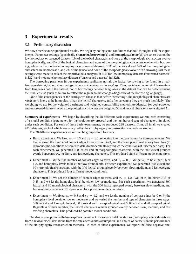
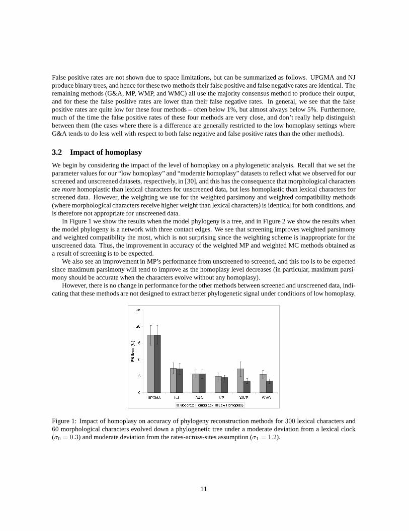
We begin by considering the impact of the level of homoplasy on a phylogenetic analysis. Recall that we set theparameter values for our “low homoplasy” and “moderate homoplasy” datasets to reflect what we observed for ourscreened and unscreened datasets, respectively, in [30], and this has the consequence that morphological charactersaremorehomoplastic than lexical characters for unscreened data, but less homoplastic than lexical characters forscreened data. However, the weighting we use for the weighted parsimony and weighted compatibility methods(where morphological characters receive higher weight than lexical characters) is identical for both conditions, andis therefore not appropriate for unscreened data.

In Figure 1 we show the results when the model phylogeny is a tree, and in Figure 2 we show the results whenthe model phylogeny is a network with three contact edges. Wesee that screening improves weighted parsimonyand weighted compatibility the most, which is not surprising since the weighting scheme is inappropriate for theunscreened data. Thus, the improvement in accuracy of the weighted MP and weighted MC methods obtained asa result of screening is to be expected.

We also see an improvement in MP’s performance from unscreened to screened, and this too is to be expectedsince maximum parsimony will tend to improve as the homoplasy level decreases (in particular, maximum parsi-mony should be accurate when the characters evolve without any homoplasy).

However, there is no change in performance for the other methods between screened and unscreened data, indi-cating that these methods are not designed to extract betterphylogenetic signal under conditions of low homoplasy.

Figure 1: Impact of homoplasy on accuracy of phylogeny reconstruction methods for300 lexical characters and60 morphological characters evolved down a phylogenetic tree under a moderate deviation from a lexical clock(σ0 = 0.3) and moderate deviation from the rates-across-sites assumption (σ1 = 1.2).

11

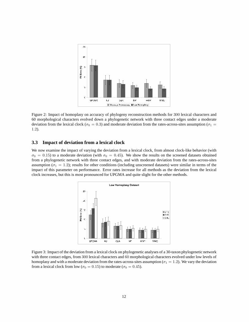
Figure 2: Impact of homoplasy on accuracy of phylogeny reconstruction methods for300 lexical characters and60 morphological characters evolved down a phylogenetic network with three contact edges under a moderatedeviation from the lexical clock (σ0 = 0.3) and moderate deviation from the rates-across-sites assumption (σ1 =1.2).

3.3 Impact of deviation from a lexical clock

We now examine the impact of varying the deviation from a lexical clock, from almost clock-like behavior (withσ0 = 0.15) to a moderate deviation (withσ0 = 0.45). We show the results on the screened datasets obtainedfrom a phylogenetic network with three contact edges, and with moderate deviation from the rates-across-sitesassumption (σ1 = 1.2); results for other conditions (including unscreened datasets) were similar in terms of theimpact of this parameter on performance. Error rates increase for all methods as the deviation from the lexicalclock increases, but this is most pronounced for UPGMA and quite slight for the other methods.

Figure 3: Impact of the deviation from a lexical clock on phylogenetic analyses of a 30-taxon phylogenetic networkwith three contact edges, from300 lexical characters and60 morphological characters evolved under low levels ofhomoplasy and with a moderate deviation from the rates-across-sites assumption (σ1 = 1.2). We vary the deviationfrom a lexical clock from low (σ0 = 0.15) to moderate (σ0 = 0.45).

12

3.4 Impact of heterotachy

In Figure 4 we show the effect on phylogenetic analyses of deviating from the rates-across-sites assumption tovarious degrees, by exploring the difference in accuracy obtained asσ1 varies from0.6 (which is close to therates-across-sites) toσ1 = 1.8 (which is further away), on data simulated on a phylogeneticnetwork with threecontact edges and low homoplasy; the same trends are observed for other model conditions. The rates-across-sitesassumption is critical to statistical models that attempt to estimate parameters under the assumption that all thesites evolve asmultiplesof each other (i.e., some faster and some slower, but with a constant ratio held betweenall sites). This is a standard assumption in phylogenetic analyses since it enables distance-based methods to bestatistically consistent under suitable conditions, and it also enables dating of internal nodes.

Interestingly, we see that asσ1 increases - i.e., as we relax the rates-across-sites assumption - methodsimprovein accuracy. The degree of improvement is small for UPGMA, and largest for the character-based methods. Oneexplanation for this is that as the rates-across-sites assumption is relaxed, the range of rates-of-change exhibitedby the set of characters on any given edge will also increase (with high probability); this, in particular, increasesthe probability that edges that are quite “short” (i.e., edgese for which t(e) is small) will exhibit some changes bysome characters, making these edges more likely to be inferred by a phylogeny reconstruction method.

Figure 4: Impact of heterotachy (deviation from the rates-across-sites assumption) on the accuracy of phylogeneticreconstruction methods on data (300 lexical characters and60 morphological characters) evolved down a phylo-genetic network with three contact edges with low homoplasy, and with moderate deviation from a lexical clock(σ0 = 0.3). The bars refer to the different values forσ1.

3.5 Varying the proportion of lexical and morphological characters

Our next analysis considered the impact of using combined datasets (both morphological and lexical together)versus lexical-only datasets, for low homoplasy levels (set to reflect the estimated homoplasy levels in [30] for the“screened” datasets). Recall that in our simulations, we set the parameters for screened morphological characters sothat there is no borrowing (this is true even of unscreened morphological characters) and so that they exhibit muchless homoplasy than lexical characters. The inclusion of morphological characters into a dataset thus reduces therate of homoplasy and borrowing. We look at four different possibilities: (a) 360 lexical and one morphological, (b)300 lexical and one morphological, (c) 300 lexical and 20 morphological, and (d) 300 lexical and 60 morphological.The comparison between (a) and (b) mostly addresses the impact of adding more data of the same type (lexical);the comparison between (b), (c) and (d) reflects the consequence of adding morphological characters to a datasetwhich is primarily lexical. Finally, the comparison between (a) and (d) allows us to see the consequence ofchoosing between lexical and morphological characters, when the total amount of data is kept fixed. In Figure 5,

13

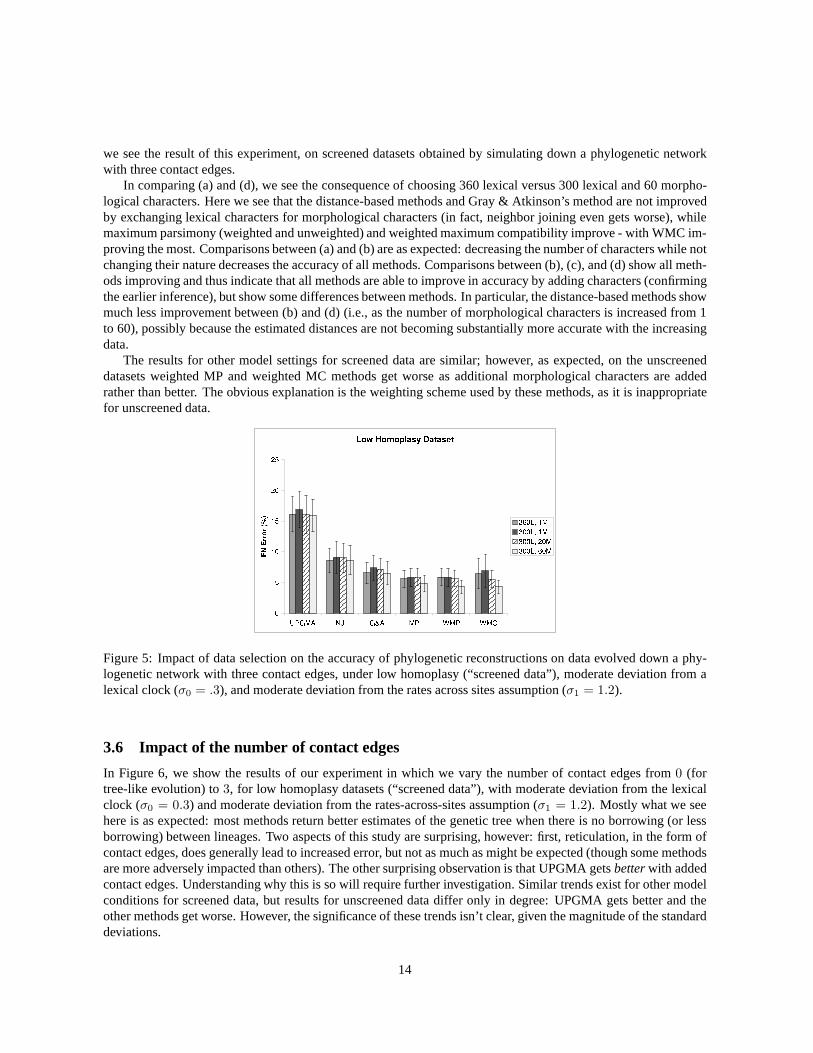
we see the result of this experiment, on screened datasets obtained by simulating down a phylogenetic networkwith three contact edges.

In comparing (a) and (d), we see the consequence of choosing 360 lexical versus 300 lexical and 60 morpho-logical characters. Here we see that the distance-based methods and Gray & Atkinson’s method are not improvedby exchanging lexical characters for morphological characters (in fact, neighbor joining even gets worse), whilemaximum parsimony (weighted and unweighted) and weighted maximum compatibility improve - with WMC im-proving the most. Comparisons between (a) and (b) are as expected: decreasing the number of characters while notchanging their nature decreases the accuracy of all methods. Comparisons between (b), (c), and (d) show all meth-ods improving and thus indicate that all methods are able to improve in accuracy by adding characters (confirmingthe earlier inference), but show some differences between methods. In particular, the distance-based methods showmuch less improvement between (b) and (d) (i.e., as the number of morphological characters is increased from 1to 60), possibly because the estimated distances are not becoming substantially more accurate with the increasingdata.

The results for other model settings for screened data are similar; however, as expected, on the unscreeneddatasets weighted MP and weighted MC methods get worse as additional morphological characters are addedrather than better. The obvious explanation is the weighting scheme used by these methods, as it is inappropriatefor unscreened data.

Figure 5: Impact of data selection on the accuracy of phylogenetic reconstructions on data evolved down a phy-logenetic network with three contact edges, under low homoplasy (“screened data”), moderate deviation from alexical clock (σ0 = .3), and moderate deviation from the rates across sites assumption (σ1 = 1.2).

3.6 Impact of the number of contact edges

In Figure 6, we show the results of our experiment in which we vary the number of contact edges from0 (fortree-like evolution) to3, for low homoplasy datasets (“screened data”), with moderate deviation from the lexicalclock (σ0 = 0.3) and moderate deviation from the rates-across-sites assumption (σ1 = 1.2). Mostly what we seehere is as expected: most methods return better estimates ofthe genetic tree when there is no borrowing (or lessborrowing) between lineages. Two aspects of this study are surprising, however: first, reticulation, in the form ofcontact edges, does generally lead to increased error, but not as much as might be expected (though some methodsare more adversely impacted than others). The other surprising observation is that UPGMA getsbetterwith addedcontact edges. Understanding why this is so will require further investigation. Similar trends exist for other modelconditions for screened data, but results for unscreened data differ only in degree: UPGMA gets better and theother methods get worse. However, the significance of these trends isn’t clear, given the magnitude of the standarddeviations.

14

Figure 6: Impact of the number of contact edges on phylogenetic reconstructions of a phylogenetic network withthree contact edges, from 360 characters (300 lexical and 60morphological) evolved under low homoplasy, mod-erate deviation from a lexical clock (σ0 = 0.3), and moderate deviation from the rates-across-sites assumption(σ1 = 1.2).

3.7 Relative performance of different methods

We turn now to the question of relative performance of different methods. Interestingly, if we exclude weightedmaximum parsimony and weighted maximum compatibility, therelative performance of the remaining methods isconsistent across all model conditions, with UPGMA the worst, NJ the next, Gray & Atkinson next, and finallyMP. The difference between the methods depends upon the model condition, but the gaps between UPGMA andNJ and between NJ and G&A are generally large, while the differences between G&A and MP are relatively small.Here we show experiments to demonstrate the conditions in which the gaps in performance between these methodsare smallest, and where they are largest.

In general, the gap in performance G&A and MP is only small when working with unscreened data (i.e.,moderate levels of homoplasy instead of low), since G&A doesn’t improve with reductions in homoplasy but MPdoes. The cases where the gap between G&A and MP is extremely small are for the unscreened data, with fewmorphological characters, and with a low deviation from therates-across-sites assumption – see, for example,Figure 8a and Figure 10a. More generally, however, the gap between G&A and MP is smallest for those modelconditions in which all methods have a harder time, whereas as the model conditions improve (for example, byincreasing the number of characters, or deviating from the rates-across-sites assumption), the gap increases. Thus,in particular, on the screened datasets, MP is clearly better than G&A.

3.8 Summary

Our study showed the following:

• There was a consistent pattern of relative accuracy of phylogenies reconstructed using these methods, withthe two distance-based methods (UPGMA and neighbor joining) less accurate than the character-based meth-ods (maximum parsimony, weighted maximum parsimony, weighted maximum compatibility, and Gray &Atkinson). UPGMA was always the worst by far.

• The relative performance within the character-based methods was often quite close, but Gray & Atkinson’smethod was always the least accurate. The only conditions under which Gray & Atkinson’s (G&A) methodwas close to Maximum Parsimony (MP) were for unscreened data.

• Deviating from the lexical clock made all methods somewhat worse, but had the biggest impact on UPGMA.

15

(a) (b)

Figure 7: Impact of the number of contact edges on phylogenetic reconstruction methods for 300 lexical charactersand 60 morphological characters, under two levels of homoplasy (moderate in (a), and low in (b)). All datasetsevolve under a moderate deviation from a lexical clock (σ0 = 0.3) and moderate deviation from the rates-across-sites assumption (σ1 = 1.2).

(a) (b)

Figure 8: Impact of the deviation from the rates across sitesassumption on phylogenetic reconstruction methods,for 300 lexical characters and 60 morphological characters, under two levels of homoplasy (moderate in (a) and lowin (b)). All characters evolve down a phylogenetic network with three contact edges under a moderate deviationfrom a lexical clock (σ0 = 0.3). We varyσ1, the parameter for deviating from the rates-across-sites assumption,from low (0.6) to moderate (1.8).

• Deviating from the rates-across-sites assumption improved the character-based methods but had little impacton the distance-based methods.

• The incidence of borrowing between languages generally made reconstructions less accurate, but not dra-matically so; surprisingly, it made UPGMA somewhat more accurate.

• The inclusion of screened morphological characters with low levels of homoplasy improves the accuracy ofall phylogeny reconstruction methods, but especially MP, WMP, and WMC.

• Using WMP and WMC on data with high levels of homoplasy produced poor results, but using WMPand WMC on data with lower levels of homoplasy (and with weights reflecting the relative resistance tohomoplasy) improved accuracy.

16

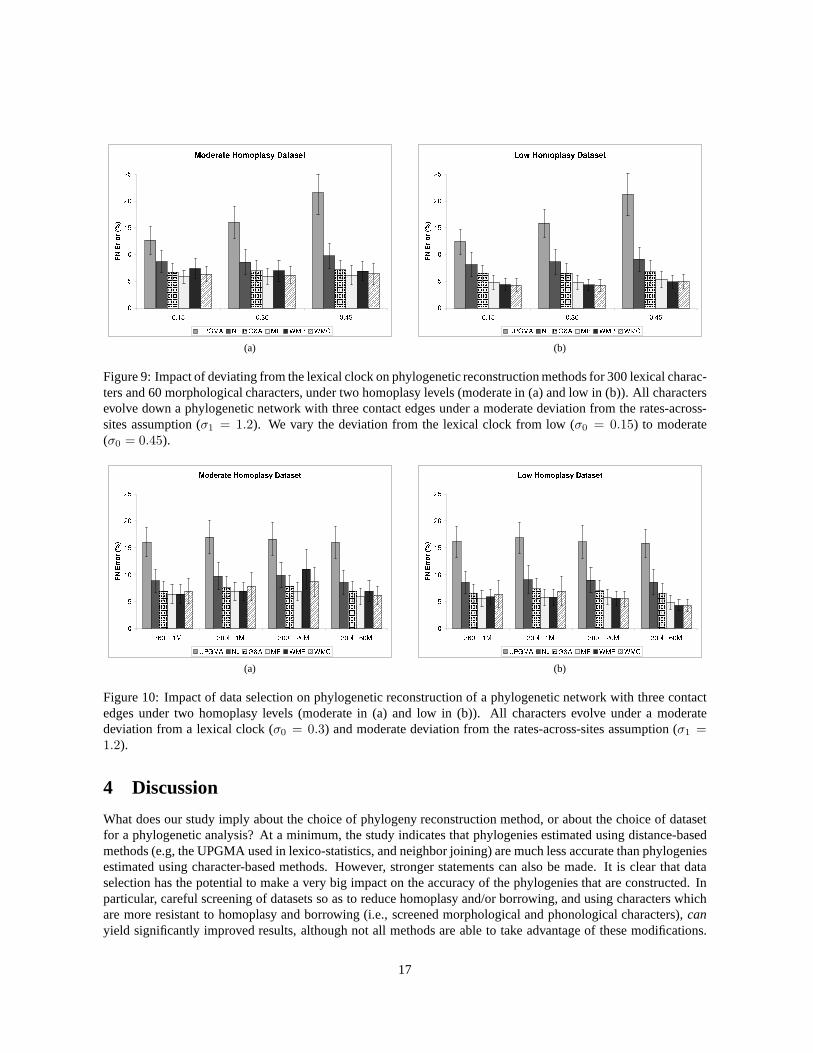
(a) (b)

Figure 9: Impact of deviating from the lexical clock on phylogenetic reconstruction methods for 300 lexical charac-ters and 60 morphological characters, under two homoplasy levels (moderate in (a) and low in (b)). All charactersevolve down a phylogenetic network with three contact edgesunder a moderate deviation from the rates-across-sites assumption (σ1 = 1.2). We vary the deviation from the lexical clock from low (σ0 = 0.15) to moderate(σ0 = 0.45).

(a) (b)

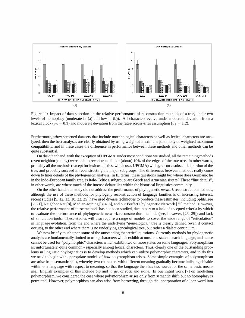
Figure 10: Impact of data selection on phylogenetic reconstruction of a phylogenetic network with three contactedges under two homoplasy levels (moderate in (a) and low in (b)). All characters evolve under a moderatedeviation from a lexical clock (σ0 = 0.3) and moderate deviation from the rates-across-sites assumption (σ1 =1.2).

4 Discussion

What does our study imply about the choice of phylogeny reconstruction method, or about the choice of datasetfor a phylogenetic analysis? At a minimum, the study indicates that phylogenies estimated using distance-basedmethods (e.g, the UPGMA used in lexico-statistics, and neighbor joining) are much less accurate than phylogeniesestimated using character-based methods. However, stronger statements can also be made. It is clear that dataselection has the potential to make a very big impact on the accuracy of the phylogenies that are constructed. Inparticular, careful screening of datasets so as to reduce homoplasy and/or borrowing, and using characters whichare more resistant to homoplasy and borrowing (i.e., screened morphological and phonological characters),canyield significantly improved results, although not all methods are able to take advantage of these modifications.

17

(a) (b)

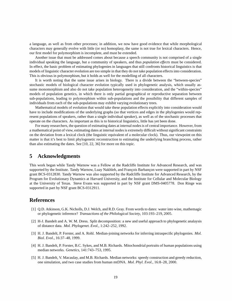
Figure 11: Impact of data selection on the relative performance of reconstruction methods of a tree, under twolevels of homoplasy (moderate in (a) and low in (b)). All characters evolve under moderate deviation from alexical clock (σ0 = 0.3) and moderate deviation from the rates-across-sites assumption (σ1 = 1.2).

Furthermore,whenscreened datasets that include morphological characters as well as lexical characters are ana-lyzed, then the best analyses are clearly obtained by using weighted maximum parsimony or weighted maximumcompatibility, and in these cases the difference in performance between these methods and other methods can bequite substantial.

On the other hand, with the exception of UPGMA, under most conditions we studied, all the remaining methods(even neighbor joining) were able to reconstruct all but (about) 10% of the edges of the true tree. In other words,probably all the methods (except for lexicostatistics, which uses UPGMA) will agree on a substantial portion of thetree, and probably succeed in reconstructing the major subgroups. The differences between methods really comedown to finer details of the phylogenetic analysis. In IE terms, these questions might be: where does Germanic liein the Indo-European family tree, is Italo-Celtic a subgroup, are Greek and Armenian sisters? These “fine details”,in other words, are where much of the intense debate lies within the historical linguistics community.

On the other hand, our study did not address the performance of phylogeneticnetworkreconstruction methods,although the use of these methods for phylogeny reconstruction of language families is of increasing interest;recent studies [9, 12, 13, 18, 22, 25] have used diverse techniques to produce these estimates, including SplitsTree[2, 21], Neighbor Net [8], Median-Joining [3, 4, 5], and our Perfect Phylogenetic Network [25] method. However,the relative performance of these methods has not been studied, due in part to a lack of accepted criteria by whichto evaluate the performance of phylogenetic network reconstruction methods (see, however, [23, 29]) and lackof simulation tools. These studies will also require a rangeof models to cover the wide range of “reticulation”in language evolution, from the end where the underlying “genealogical” tree is clearly defined (even if contactoccurs), to the other end where there is no underlying genealogical tree, but rather a dialect continuum.

We now briefly touch upon some of the outstanding theoreticalquestions. Currently methods for phylogeneticanalysis are fundamentally limited to using characters which exhibit at most one state on each language, and hencecannot be used for “polymorphic” characters which exhibit two or more states on some languages. Polymorphismis, unfortunately, quite common - especially among lexicalcharacters. Thus, clearly one of the outstanding prob-lems in linguistic phylogenetics is to develop methods which can utilize polymorphic characters, and to do thiswe need to begin with appropriate models of how polymorphismarises. Some simple examples of polymorphismare arise from semantic shift, whereby two characters with different meaning gradually become indistinguishablewithin one language with respect to meaning, so that the language then has two words for the same basic mean-ing. English examples of this includebig and large, or rock and stone. In our initial work [7] on modellingpolymorphism, we considered the case where polymorphism arises only from semantic shift, but no homoplasy ispermitted. However, polymorphism can also arise from borrowing, through the incorporation of a loan word into

18

a language, as well as from other processes; in addition, we now have good evidence that while morphologicalcharacters may generally evolve with little (or no) homoplasy, the same is not true for lexical characters. Hence,our first model for polymorphism is incomplete, and must be extended.

Another issue that must be addressed comes about because a speech community is not comprised of a singleindividual speaking the language, but a community of speakers, and thuspopulation effectsmust be considered.In effect, the basic problem of estimating phylogenies in languages that still confronts historical linguistics is thatmodels of linguistic character evolution are too simple in that they do not take population effects into consideration.This is obvious in polymorphism, but it holds as well for the modelling of all characters.

It is worth noting that the same issue arises in biology. There is a divide between the “between-species”stochastic models of biological character evolution typically used in phylogenetic analysis, which usually as-sume monomorphism and also do not take population heterogeneity into consideration, and the “within-species”models of population genetics, in which there is only partial geographical or reproductive separation betweensub-populations, leading to polymorphism within sub-populations and the possibility that different samples ofindividuals from each of the sub-populations may exhibit varying evolutionary trees.

Mathematical models of evolution that would take these population effects explicitly into consideration wouldhave to include modifications of the underlying graphs (so that vertices and edges in the phylogenies would rep-resent populations of speakers, rather than a single individual speaker), as well as of the stochastic processes thatoperate on the characters. As important as this is to historical linguistics, little has yet been done.

For many researchers, the question of estimating dates at internal nodes is of central importance. However, froma mathematical point of view, estimating dates at internal nodes is extremely difficult without significant constraintson the deviation from a lexical clock (the linguistic equivalent of a molecular clock). Thus, our viewpoint on thismatter is that it’s best to limit phylogenetic reconstruction to estimating the underlying branching process, ratherthan also estimating the dates. See [10, 22, 36] for more on this topic.

5 Acknowledgments

This work began while Tandy Warnow was a Fellow at the Radcliffe Institute for Advanced Research, and wassupported by the Institute. Tandy Warnow, Luay Nakhleh, andFrancois Barbancon were supported in part by NSFgrant BCS-0312830. Tandy Warnow was also supported by the Radcliffe Institute for Advanced Research, by theProgram for Evolutionary Dynamics at Harvard University, and the Institute for Cellular and Molecular Biologyat the University of Texas. Steve Evans was supported in partby NSF grant DMS-0405778. Don Ringe wassupported in part by NSF grant BCS-0312911.

References

[1] Q.D. Atkinson, G.K. Nicholls, D.J. Welch, and R.D. Gray.From words to dates: water into wine, mathemagicor phylogenetic inference?Transactions of the Philological Society, 103:193–219, 2005.

[2] H-J. Bandelt and A. W. M. Dress. Split decomposition: a new and useful approach to phylogenetic analaysisof distance data.Mol. Phylogenet. Evol., 1:242–252, 1992.

[3] H. J. Bandelt, P. Forster, and A. Rohl. Median-joining networks for inferring intraspecific phylogenies.Mol.Biol. Evol., 16:37–48, 1999.

[4] H. J. Bandelt, P. Forster, B.C. Sykes, and M.B. Richards.Mitochondrial portraits of human populations usingmedian networks.Genetics, 141:743–753, 1995.

[5] H. J. Bandelt, V. Macaulay, and M.B. Richards. Median networks: speedy construction and greedy reduction,one simulation, and two case studies from human mtDNA.Mol. Phyl. Evol., 16:8–28, 2000.

19

[6] O. Bininda-Emonds, S. Brady, J. Kim, and M. Sanderson. Scaling of accuracy in extremely large phylogenetictrees. InProc. 6th Pacific Symposium on Biocomputing (PSB01), pages 547–557. World Scientific, 2001.

[7] M. Bonet, C.A. Phillips, T. Warnow, and S. Yooseph. Constructing evolutionary trees in the presence ofpolymorphic characters.SIAM J. Computing, 29(1):103–131, 1999. (A preliminary version appeared in theACM Symposium on the Theory of Computing, 1996.).

[8] D. Bryant and V. Moulton. Neighbor-net: an agglomerative method for the construction of phylogeneticnetworks.Molecular Biology and Evolution, 21:255–265, 2003.

[9] D. Bryant and M. Steel. Fast algorithms for constructingoptimal trees from quartets.J. Algs., 38(1):xxx–xxx,2001.

[10] S.N. Evans and T. Warnow. Unidentifiable divergence times in rates-across-sites models.IEEE/ACM Trans-actions on Computational Biology and Bioinformatics, 1:130–134, 2005.

[11] J. Felsenstein.Inferring Phylogenies. Sinauer Associates, Sunderland, Massachusetts, 2004.

[12] P. Forster, T. Polzin, and A. Rohl. Evolution of Englishbasic vocabulary within the network of Germaniclanguages. In P. Forster and C. Renfrew, editors,Phylogenetic Methods and the Prehistory of Languages,pages 131–138. McDonald Institute for Archaeological Research, 2006.

[13] P. Forster and A. Toth. Towards a phylogenetic chronology of ancient Gaulish, Celtic, and Indo-European.Proceedings of the National Academy of Sciences, 100(15):9079–9084, 2003.

[14] R. Gray and Q.D. Atkinson. Language-tree divergence times support the Anatolian theory of Indo-Europeanorigin. Nature, 426:435–439, 2003.

[15] D. M. Hillis, J. P. Huelsenbeck, and D. L. Swofford. Hobgoblin of phylogenetics.Nature, 369:363–364,1994.

[16] H.M. Hoenigswald.Language Change and Linguistic Reconstruction. University of Chicago Press, Chicago,1960.

[17] C.J. Holden. Bantu language trees reflect the spread of farming across sub-Saharan Africa: a maximum-parsimony analysis.Proceedings of the Royal Society of London, Series B, 269:793–9, 2002.

[18] C.J. Holden and R. Gray. Rapid radiation, borrowing, and dialect continua in the Bantu languages. InP. Forster and C. Renfrew, editors,Phylogenetic Methods and the Prehistory of Languages, pages 19–32.McDonald Institute for Archaeological Research, 2006.

[19] J. P. Huelsenbeck and D. M. Hillis. Success of phylogenetic methods in the four-taxon case.Syst. Biol.,42:247–264, 1993.

[20] J.P. Huelsenbeck and R. Ronquist. MrBayes: Bayesian inference of phylogeny.Bioinformatics, 17:754–755,2001.

[21] D. H. Huson. SplitsTree: A program for analyzing and visualizing evolutionary data.Bioinformatics,14(1):68–73, 1998.

[22] A. McMahon and R. McMahon. Why linguists don’t do dates:evidence from Indo-European and Australianlanguages. In P. Forster and C. Renfrew, editors,Phylogenetic Methods and the Prehistory of Languages,pages 153–160. McDonald Institute for Archaeological Research, 2006.

20

[23] B.M.E. Moret, L. Nakhleh, T. Warnow, C.R. Linder, A. Tholse, A. Padolina, J. Sun, and R. Timme. Phy-logenetic networks: modeling, reconstructibility, and accuracy. IEEE/ACM Transactions on ComputationalBiology and Biocomputing, 1(1), 2004.

[24] L. Nakhleh, B. M. E. Moret, U. Roshan, K. St. John, J. Sun,and T. Warnow. The accuracy of fast phylogeneticmethods for large datasets. InProc. 7th Pacific Symposium on Biocomputing (PSB02), pages 211–222. WorldScientific, 2002.

[25] L. Nakhleh, D. Ringe, and T. Warnow. Perfect phylogenetic networks: A new methodology for reconstructingthe evolutionary history of natural languages.Language (Journal of the Linguistic Society of America),81(2):382–420, 2005.

[26] L. Nakhleh, U. Roshan, K. St. John, J. Sun, and T. Warnow.The performance of phylogenetic methods ontrees of bounded diameter. InProceedings of the 1st Workshop on Algorithms in Bioinformatics (WABI),2001. Aarhus, Denmark.

[27] L. Nakhleh, U. Roshan, K. St. John, J. Sun, and T. Warnow.The accuracy of phylogenetic methods for largedatasets. InProceedings of the Pacific Symposium on Biocomputing (2002), pages 211–222, 2002. Kauai,Hawaii.

[28] L. Nakhleh, U. Roshan, K. St. John, J. Sun, and T. Warnow.Designing fast converging phylogenetic methods.Bioinformatics, 17:190S–198S, 2001.

[29] L. Nakhleh, J. Sun, T. Warnow, C.R. Linder, B.M.E. Moret, and A. Tholse. Towards the development ofcomputational tools for evaluating phylogenetic network reconstruction methods. InProc. 8th Pacific Symp.on Biocomputing (PSB 2003), 2003.

[30] L. Nakhleh, T. Warnow, D. Ringe, and S.N. Evans. A comparison of phylogenetic reconstruction methods onan IE dataset.The Transactions of the Philological Society, 3(2):171–192, 2005.

[31] G.K. Nicholls and R.D. Gray. Dated ancestral trees frombinary trait data.Unpublished, 2006.

[32] D. Ringe, T. Warnow, and A. Taylor. Indo-European and computational cladistics.Transactions of thePhilological Society, 100(1):59–129, 2002.

[33] D. F. Robinson and L. R. Foulds. Comparison of phylogenetic trees.Mathematical Biosciences, 53:131–147,1981.

[34] N. Saitou and M. Nei. The neighbor-joining method: A newmethod for reconstructing phylogenetic trees.Molecular Biology and Evolution, 4:406–425, 1987.

[35] M. Sanderson. r8s software package. http://loco.ucdavis.edu/r8s/r8s.html.

[36] D. Ringe S.N. Evans and T. Warnow. Inference of divergence times as a statistical inverse problem. InP. Forster and C. Renfrew, editors,Phylogenetic Methods and the Prehistory of Languages, pages 119–130.MacDonald Institute for Archaeological Research, 2006.

[37] D. Swofford. PAUP*: Phylogenetic analysis using parsimony (and other methods), version 4.0. 1996.

[38] D.L. Swofford, G.J. Olsen, P.J. Waddell, and D.M. Hillis. Phylogenetic inference. In D.M. Hillis, C. Moritz,and B.K. Mable, editors,Molecular Systematics. Sinauer Associates, Sunderland, Massachusetts, 1996.

[39] T. Warnow, S.N. Evans, D. Ringe, and L. Nakhleh. A stochastic model of language evolution that incorporateshomoplasy and borrowing. In P. Forster and C. Renfrew, editors, Phylogenetic Methods and the Prehistoryof Languages, pages 75–90. MacDonald Institute for Archaeological Research, 2006.

21

Appendix

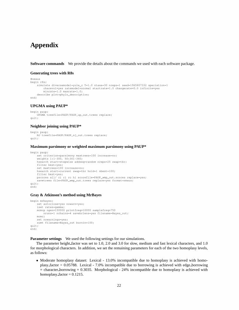
Software commands We provide the details about the commands we used with each software package.

Generating trees with R8s#nexusbegin r8s;

simulate diversemodel=yule_c T=1.0 ntaxa=30 nreps=1 seed=1965807332 speciation=1charevol=yes ratemodel=normal startrate=1.0 changerate=0.0 infinite=yesminrate=1.0 maxrate=1.0;

describe plot=phylo_description;end;

UPGMA using PAUP*begin paup;

UPGMA treefile=PAUP/PAUP_up_out.trees replace;quit;

Neighbor joining using PAUP*begin paup;

NJ treefile=PAUP/PAUP_nj_out.trees replace;quit;

Maximum parsimony or weighted maximum parsimony using PAUP*begin paup;

set criterion=parsimony maxtrees=100 increase=no;weights 1:1-300, 50:301-360;hsearch start=stepwise addseq=random nreps=25 swap=tbr;filter best=yes;set maxtrees=100 increase=no;hsearch start=current swap=tbr hold=1 nbest=100;filter best=yes;pscores all/ ci ri rc hi scorefile=PAUP_wmp_out.scores replace=yes;savetrees file=PAUP_wmp_out.trees replace=yes format=nexus;

quit;end;

Gray & Atkinson’s method using MrBayesbegin mrbayes;

set autoclose=yes nowarn=yes;lset rates=gamma;mcmcp ngen=150000 printfreq=10000 samplefreq=750

nruns=1 nchains=4 savebrlens=yes filename=Bayes_out;mcmc;set nowarnings=yes;sumt filename=Bayes_out burnin=100;

quit;end;

Parameter settings We used the following settings for our simulations.The parameter heightfactor was set to 1.0, 2.0 and 3.0 for slow, medium and fast lexical characters, and 1.0

for morphological characters. In addition, we set the remaining parameters for each of the two homoplasy levels,as follows:

• Moderate homoplasy dataset: Lexical - 13.0% incompatible due to homoplasy is achieved with homo-plasy factor = 0.05788. Lexical - 7.0% incompatible due to borrowing is achieved with edgeborrowing= characterborrowing = 0.3035. Morphological - 24% incompatible due tohomoplasy is achieved withhomoplasyfactor = 0.1215.

22

• Low homoplasy dataset: Lexical - 1.0% incompatible due to homoplasy is achieved with homoplasyfactor= 0.01321. Lexical - 6.0% incompatible due to borrowing is achieved with edgeborrowing = charac-ter borrowing = 0.281425. Morphological - no borrowing, no homoplasy, so homoplasyfactor - 0.0 =edgeborrowing= characterborrowing.

23