An Experimental Investigation of A Passive Cooling Unit ...

An Experimental Investigation of A Passive Cooling Unit for Nuclear

Plant Containment

by

Haiyang Liu

B.S., Engineering Physics, Tsinghua University, 1993

Submitted to the Department of Mechanical Engineering and the

Department of Nuclear Engineering in Partial Fulfillment of the

Requirements for the Degrees of

Master of Science in Mechanical Engineering

and

Master of Science in Nuclear Engineering

at the MASSACHUSETTS INSTITUTEMassachusetts Institute of Technology

February 1999

© 1999 Massachusetts Institute of Technology

All rights reserved QSignature of A uthor.......................................................... ....... ...... ......... ........................

Dep n of Nuclear EngineeringFebruary 4, 1999

Certified by....................................................... .- ......

Professor Neil E. Todreas

Thesis Supervisor, Deartment of Nuclear Engineering

Certified by....................... .Professor Emeritus Michael J. Driscoll

Thesis rvisorg partment of Nuclear Engineering

C ertified by...................................... ....................49ffessor Emeritus Peter Griffith

Thesis Reader, Departmept of Mechanical Engineering

A ccepted by............................................................... .... c

Chairman, Department Graduate Committpeibept. of Nucl. Eng.

A ccepted by.................................................................

Professor Ain A. Sonin

Chairman, Department Committee on Graduate Students, Dept. of Mech. Eng.

An Experimental Investigation of A Passive Cooling Unit for NuclearPlant Containment

byHaiyang Liu

Submitted to the Department of Nuclear Engineering and theDepartment of Mechanical Engineering On February 4, 1999 in

Partial Fulfillment of the Requirements for the Degrees ofMaster of Science in Nuclear Engineering

andMaster of Science in Mechanical Engineering

ABSTRACT

A set of condensation experiments in the presence of noncondensables (e.g. air, helium)were conducted to evaluate the heat removal capacity of a passive cooling unit in a post-accident containment.

Condensation heat transfer coefficients on a vertically mounted smooth tube have beenobtained for total pressure ranging from 36 psia to 66 psia, and air mass fraction rangingfrom 0.30 to 0.65. An empirical correlation has been developed in term of a parametergroup made up of steam mole fraction(Xs), total pressure(P), temperature differencebetween bulk gas and wall surface (dT). This correlation covers all data points within20%. All data points are also in good agreement with the prediction of the Diffusion LayerModel (DLM) with suction. The effect of helium (simulating hydrogen) on heat transfercoefficient was investigated for helium mole fraction in noncondensable gases Xhe/Xnc at15%, 30% and 60%. It was found that the condensation heat transfer coefficients are gen-erally lower when introducing helium into noncondensable gas. The difference is within20% of air-only cases when Xhe/Xnc is less than 30% and total pressure is less than 66psia. A gas stratification phenomenon was clearly observed for helium mole fraction inexcess of 60%. The limiting case of the shadowing effect in a tube bundle has been inves-tigated by adding a shroud around the smooth tube. It was found that the average heatremoval capability is reduced by a factor of 0.6.

A made-in-house axial-finned tube and a commercial radial-finned tube, which was origi-nally designed for forced air cooling, have been tested under conditions similar to thesmooth tube. An enhancement factor of 1.5 to 2 for the axial-finned tube and 1.0 to 1.5 forthe radial-finned tube have been obtained. The reasons for the less-than-optimal perfor-mance of these finned tubes are discussed.

Thesis Supervisor: Neil E. TodreasTitle: Professor of Nuclear Engineering

2

Thesis Supervisor: Michael J. DriscollTitle: Professor Emeritus of Nuclear Engineering

3

Acknowledgments

I am indebted to a number of people who helped me through this arduous and challenging

research project.

My advisors, Prof. Todreas and Prof. Driscoll deserve high praise for their academic guid-

ance and continued support throughout this work. I also wish to thank Prof. Griffith, my

thesis reader, for his advice on identifying the right approach in the experimental investi-

gation.

My appreciation is also due to Dr. Gordon Kohse in the MIT Reactor Laboratory and Peter

Stahle in the MIT Fusion Center for their valuable suggestions and efforts in setting up the

experimental apparatus.

The financial sponsorship of the Korea Electric Power Corporation and MIT are gratefully

acknowledged.

Special thanks are directed towards my family in China and my friend, Yi Zhang, at MIT

for their long-term spiritual support.

4

Table of Contents

Title Page............................................................................................................................. 1ABSTRA CT........................................................................................................................ 2A cknow ledgm ents............................................................................................................... 4Table of Content .................................................................................................................. 5List of Figures......................................................................................................................7List of Tables.......................................................................................................................8N om enclature......................................................................................................................9Chapter 1 Introduction............................................................................................. 12

1.1 M otivation ............................................................................................................. 121.2 Scope of Current Work and Organization of This Report.................................171.3 Sum m ary................................................................................................................18

Chapter 2 Literature Review for Steam Condensation with Noncondensables ..... 192.1 Sm ooth Surfaces ................................................................................................. 19

2.1.1U chida & Tagam i ......................................................................................... 202.1.2G ido & Koestel.............................................................................................202.1.3D ehbi.............................................................................................................212.1.4Peterson & Corradini .................................................................................... 22

2.2 Profiled Surfaces............................................................................................... 242.2.1 Pure Steam Condensation ............................................................................. 242.2.2Condensation w ith N oncondensable G ases ............................................. 25

2.3 Sum m ary................................................................................................................26Chapter 3 D esign of Experim ent............................................................................ 28

3.1 Introduction ....................................................................................................... 283.1.1Aim ............................................................................................................... 283.1.2D esign Strategy........................................................................................ 283.1.3M easurem ent Strategy .............................................................................. 29

3.2 Experim ental Apparatus ................................................................................... 313.2.1 General view of the experim ental setup ................................................... 313.2.2Instrum entation ........................................................................................ 323.2.3D ata A cquisition System .......................................................................... 32

3.3 Operation Procedure .............................................................................................. 363.3.1 Calibration of M easurem ent D evices ........................................................ 363.3.2A djustm ent of Operating Conditions........................................................ 363.3.3 D ata Collection and Processing ............................................................... 37

3.4 Sum m ary................................................................................................................37Chapter 4 Results and Discussion for Smooth Tube ............................................... 38

4.1 Test M atrix ....................................................................................................... 384.2 Repeatability of Experim ents ............................................................................ 394.3 Condensation in the Presence of Air Only ....................................................... 39

5

4.3.1Empirical Correlation from Experimental Data...................394.3.2Comparison of the Experimental Data to Theoretical Analysis .............. 404.3.3Comparison of the Experimental Data to Existing Correlations and Models...

43

4.4 Condensation in the Presence of Air and Helium............................................. 444.5 Shadowing Effect in a Tube Bundle................................................................. 454.6 Sum m ary ................................................................................................................ 46

Chapter 5 Results and Discussion for Finned Tubes...............................................635.1 Introduction ....................................................................................................... 635.2 Finned Tube Parametric Design Based on Theoretical Analysis ...................... 63

5.2.1 R adial-finned Tube ................................................................................... 645.2.2A xial Finned Tube ................................................................................... 69

5.3 Results and Discussions of Finned Tubes Tests ............................................... 725.3. 1A xial-finned Tube..................................................................................... 725.3.2R adial-finned Tube ................................................................................... 73

5.4 S um m ary ................................................................................................................ 73Chapter 6 Summary, Conclusions and Recommendations ..................................... 81

6.1 Summary and Conclusions ................................................................................ 816.2 Recommendations for Future Work ................................................................. 82

R eferences...................................................................................................................... 84Appendix A Data for Smooth Tube Air-Steam Runs .................................................... 87Appendix B Data for Smooth Tube Air-Helium-Steam Runs .................. 89Appendix C Data for Smooth Tube Air-Steam Runs With Shroud..............90Appendix D Data for Axial-finned Tube Air-Steam Runs .................... 91Appendix E Data for Radial-finned Tube Air-Steam Runs ................... 92Appendix F Suppliers of Primary Components........................................................ 93Appendix G Data Reduction and Error Analysis Procedure ..................................... 95Appendix H Standard Operating Procedure (SOP) ....................................................... 99Appendix I Code for Data Reduction ......................................................................... 103

6

List of Figures

Figure 1.1 The closed two-phase thermosyphon loop for cooling a double walled concretePW R containm ent ....................................................................................................... 14Figure 1.2 Schematic of the IEO Conceptual Design.................................................15Figure 3.1 Schematic of the Steam Condensation Experiment in the Presence of Air...30Figure 3.2 Schematic of the Thermocouple Distribution on the Smooth Test Section ..34Figure 3.3 Schematic of Data Acquisition System...................................................35Figure 4.1 Empirical Correlation of Air Noncondensable Runs for Smooth Tube ........ 47Figure 4.2 Correlation of Vertical Wall Data Reduced From Air Noncondensable Runs forSmooth Tube Based on Pure Natural Convection Model..........................................48Figure 4.3 Correlation of Vertical Wall Data Reduced From Air Noncondensable Runs forSmooth Tube Based on Equimolal Counterdiffusion Model......................................49Figure 4.4 Correlation of Vertical Wall Data Reduced From Air Noncondensable Runs forSmooth Tube Based on Diffusion through Stationary Gas Layer Model..................50Figure 4.5 Comparison of Vertical Wall Data Reduced from Air Noncondensable Runs forSmooth Tube against DLM with Suction ....................................................................... 51Figure 4.6 Comparison of Vertical Wall Data Reduced from Air Noncondensable Runs forSmooth Tube against DLM without Suction .................................................................. 52Figure 4.7 Comparison of Vertical Wall Data Reduced from Air Noncondensable Runs forSmooth Tube against Uchida Correlation................................................................... 53Figure 4.8 Comparison of DLM (With Suction) against 2.2*Uchida Correlation ......... 54Figure 4.9 Comparison of Vertical Wall Data Reduced from Air Noncondensable Runs forSmooth Tube against Dehbi Correlation................................................................... 55Figure 4.10 Helium Effect on Heat Transfer Coefficient at Pt=3.5 atm....................56Figure 4.11 Helium Effect on Heat Transfer Coefficient at Pt=4.5 atm....................57Figure 4.12 Helium Effect on Heat Transfer Coefficient at Xsteam=0.61................58Figure 4.13 Axial Temperature Distribution of Atmosphere Inside Vessel..............59Figure 4.14 Repeatability of Smooth Tube Air-only Experiment Data at Pt=3 atm......60Figure 4.15 Shroud Effect on Heat Transfer Coefficient at Pt=3.5 atm.....................61Figure 4.16 Shroud Effect on Heat Transfer Coefficient at Wair=0.52 .................... 62Figure 5.1 Radial-fin Enhancement Factor Changes with Geometry ........................ 68Figure 5.2 Radial-fin Efficiency Changes with Geometry ....................................... 68Figure 5.3 Axial-fin Enhancement Factor Changes with Geometry...........................70Figure 5.4 Axial-fin Efficiency Changes with Geometry .......................................... 70Figure 5.5 The Proposed Finned Tube Designs.......................................................... 71Figure 5.6 Schematic of the Tested Axial-finned Tube............................................75Figure 5.7 Schematic of the Tested Radial-finned Tube ............................................ 76Figure 5.8 Enhancement Factors of the Axial-finned Tube at Wair=0.54 ................ 77Figure 5.9 Enhancement Factors of the Axial-finned Tube at Pt=4.5 atm.................78Figure 5.10 Enhancement Factors of the Radial-finned Tube at Wair=O.50..............79Figure 5.11 Enhancement Factors of the Radial-finned Tube at Pt=4.5 atm..............80

7

List of TablesTable 1.1 Design Data of the Initial Representative Thermosyphon Loop......................16Table 1.2 Key Features of the Proposed IEO Design......................................................17Table 2.1 Key Features of the Evaporator Finned-Tube Designed by ENEL.................27Table 4.1 Matrix of Smooth Tube Pure Air Runs..........................................................38Table 4.2 Matrix of Smooth Tube Air-Helium Runs......................................................39Table 4.3 Matrix of Runs for Smooth Tube with Shroud...............................................45Table 5.1 The Constants Used in Estimating the Performance of the Finned Tubes.....67Table 5.2 Features of the Proposed Radial-finned Tube for the Evaporator....................67Table 5.3 Features of the Proposed Axial-finned Tube for the Evaporator....................72Table 5.4 Summary of Enhancement Factors for Proposed and Tested Finned Tubes........74Table A. 1 Data for Smooth Tube Air-Steam Runs........................................................87Table B.1 Data for Smooth Tube Air-Helium-Steam Runs................................................89Table C. 1 Data for Smooth Tube Air-Steam Runs With Shroud....................................90Table D. 1 Data for Axial-finned Tube Air-Steam Runs...............................................91Table E. 1 Data for Radial-finned Tube Air-Steam Runs...............................................92Table F. 1 Suppliers of Primary Components................................................................. 93Table H. 1 List of Alarm Lights and Actions to Be Taken.................................................102Table H.2 List of Instrument Devices Related to Power-on Run......................................102

8

Nomenclature

General NotationA, S flow area (M2 )B loop breadth (m)CP specific heat capacity for constant pressure (J/kgK)D duct diameter (m)d tube diameter (m)f friction factor (-)G mass flux (kg/m2)Gr Grashof number (-)g gravitational acceleration (m/s2)H loop height (m)H modified heat transfer coefficient (W/m2 K)h heat transfer coefficient (W/m2K)hfg latent heat (J/kg)K form loss factor (-)k thermal conductivity (W/mK)L length (m)rih mass flow rate (-)N number of heat exchanger tubes (-)n number of fins (-)Nu Nusselt number (-)P perimeter (m)Pr Prandtl number (-)P pressure (Pa)Pt total pressureQ thermal power (W)4" heat flux (W/m2)Ra Rayleigh number (-)Re Reynolds number (-)Rb radius of base tube (m)Rout radius of the outer edge of a radial fin (m)s longitudinal coordinate (m)T temperature(*C)t fin thickness (m)U overall heat transfer coefficient (W/m2K)u velocity (m/s)v specific volume (m3/kg)x vapor quality (-)z altitude coordinate (m)

9

Greek SymbolsP thermal expansion coefficient (K-1)AT temperature difference (K)6 tube wall thickness (m)E fin effectiveness

dynamic viscosity (kg/ms)V kinematic viscosity (m2/s)p density (kg/M3)(D fin efficiency (-)X fin enhancement factor0 temperature difference (K)0 angle (0)a surface tension (N/m)'t shear stress (N/m 2)

Subscriptsair moist air

av average

b basis

C condenser

CB convective boiling

c cross-sectional area

cond condensate

cont containment

cro cross section

E evaporator

e exit

el electrical power

FC forced convection

FZ Forster-Zuber

f fluid (liquid)

fg difference between fluid and gas property

fin fin on the tube outside

form form losses

fric wall friction losses

g gas (vapor)

high higher valuein inside, input

L referred to the length L

low lower value

NB nucleate boiling

SP single-phase

sat saturated liquid mode

sep separator

steam steam

10

TP two-phaseth thermal powertrans transported energytube tube

t total

Uchida Uchida correlationw wallwin wall insideout wall outside

8 condensate film

1,2,3,4 loop section index

11

Chapter 1

Introduction

1.1 Motivation

With the public's increasing concerns over environmental problems, the safety of nuclear

plants has become a critical issue for the future of nuclear energy. As the last of the several

barriers to the escape of radioactive species, high integrity containment has been one of

the most active design focuses in recent years. In particular, to mitigate external hazard

effects, including airplane crashes and pressure waves, and the internal effects of hypo-

thetical severe accidents (e.g. LOCA and MSLB), a double-wall concrete containment

configuration is preferred for future nuclear plants in Korea and Europe.

However, it is difficult to remove the energy released in severe accidents from a con-

crete containment due to the low thermal conductivity of concrete. A containment cooling

system with high thermal conductance devices has to be incorporated. To best survive and

function in the harsh after-accident condition, this system is preferably completely pas-

sive(i.e. completely independent from any mechanical, electrical and Instrumentation &

Control system, which might not work after a severe accident). A system of this type, a so-

called passive containment cooling system (PCCS) is the subject of the work reported in

this thesis.

A variety of candidate PCCSs have been studied to date. Notable systems are:

1. Temperature-Initiated Passive Cooling System(TIPACS) by ORNL [9]

2. Heat pipe design for a passive containment heat removal system by UCLA[ 11] [12]

3. Thermosyphon loop concept for double-shell concrete containment by ENEL[10]

12 Chapter I Introduction

A thermosyphon type design, sketched in Figure 1.1, has been investigated at MIT.

The basic feasibility of closed two-phase thermosyphon loops for passive containment

cooling has been confirmed and calculation shows that an approximately 5-10 MW heat

removal capacity could be obtained for units with the characteristics in Table 1.1 [13].

More recently an Internal Evaporator Only (IEO) concept which vents steam to the atmo-

sphere has been investigated [14] since it reduces the number of in-containment IEO loops

required. The schematic of this design is shown in Figure 1.2. Table 1.2 lists its key fea-

tures.

Numerical computation has shown that the critical factor influencing system perfor-

mance is the shell-side condensation heat transfer because of the existence of a large con-

centration of noncondensables (e.g. air, hydrogen), which can not be removed as in most

other industrial applications. The need for correlations directly applicable to post-LOCA

containment conditions motivated evaporator tube experiments to investigate the perfor-

mance of our conceptual designs.

To improve performance, heat transfer enhancement means have been considered.

There are generally two types of enhancement methods: increasing heat transfer area and

increasing heat transfer coefficient. In our case since it is impossible to remove noncon-

densables, it is harder to increase the heat transfer coefficient. So far no literature reported

if the dropwise condensation mechanism would help in a condition with a large amount of

noncondensables. Further surface treatment techniques used in industry for dropwise con-

densation are complicated and can not guarantee a long-lasting stable performance. Thus

the recent work has concentrated on increasing heat transfer area by using finned tubes.

Both axial-finned and radial-finned tubes have been investigated in our experiments. The

measured enhancement factor compared to smooth tube results can be used in contain-

ment performance analysis codes such as GOTHIC to evaluate the use of a PCCS to insure

containment integrity.

1.1 Motivation 13

1.1 Motivation 13

double walled concretecontainment building

saturated-steam air mixture water poolafter LOCA or MSLB

T~ = 140 *CT""10 TO, = 60 *C

CondenserQ. lm:: +:: with Nc tubes

steam -:- OutH-

Lc

Evaporatorwith NE tubes

z0Qn

LE

liquid

B

NOT TO SCALE

Figure 1.1 The closed two-phase thermosyphon loop for cooling a double

walled concrete PWR containment

14 Chapter 1 Introduction


Steam Exhaust

..m.._I

_________________ $

separator

Mixing Plenlum

tEmto

On-set of- Boiling

- SubcoolecBolitng

14.5

13.5 -

- 8m

5.1..

-- 2.5m -

0.7m - -

- 0.5 m

0.2 m F3

4 -Om

2 12 m

hsI

water level

T.. T

PSCS Tank

H

Figure 1.2 Schematic of the IEO Conceptual Design

1.1 Motivation 15

RecrculatiLine

9 M

21

15

44 2.5 m

1. 1 Motivation

Table 1.1 Design Data of the Initial Representative Thermosyphon Loop

Parameters Value

Main loop geometryLoop Height H = 12 mLoop Breadth B = 5 mEvaporator Length LE = 5 mCondenser Length Lc = 5 mHeight of the evaporator entrance z1 = 1 mHeight of condenser exit zo = 1 mDiameter of the lower duct D, = 0.1 mDiameter of the upper duct D 3 = 0.3 m

Evaporator heat exchangerTube Length LE = 5 mInner tube diameter dE = 0.03 mTube wall thickness 5E= 1 mmNumber of evaporator tubes NE = 500Inner surface of a single tube AE = 0.47 m 2

Total heat exchanger surface AEt = 236 m2

Condenser heat exchangerTube Length Lc = 5 mInner tube diameter dc = 0.03 mTube wall thickness 8c= 1 mmNumber of condenser tubes Nc = 368Inner surface of a single tube AC = 0.47 m 2

Total heat exchanger surface Act = 173 m2



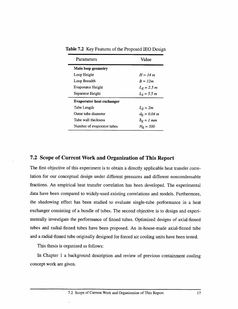
Table 7.2 Key Features of the Proposed IEO Design

Parameters Value

Main loop geometry

Loop Height H = 14 m

Loop Breadth B = 12m

Evaporator Height LE = 2.5 m

Separator Height Ls = 5.5 m

Evaporator heat exchanger

Tube Length LE = 2m

Outer tube diameter dE = 0.04 m

Tube wall thickness 8 E = 1 mm

Number of evaporator tubes NE = 500

7.2 Scope of Current Work and Organization of This Report

The first objective of this experiment is to obtain a directly applicable heat transfer corre-

lation for our conceptual design under different pressures and different noncondensable

fractions. An empirical heat transfer correlation has been developed. The experimental

data have been compared to widely-used existing correlations and models. Furthermore,

the shadowing effect has been studied to evaluate single-tube performance in a heat

exchanger consisting of a bundle of tubes. The second objective is to design and experi-

mentally investigate the performance of finned tubes. Optimized designs of axial-finned

tubes and radial-finned tubes have been proposed. An in-house-made axial-finned tube

and a radial-finned tube originally designed for forced air cooling units have been tested.

This thesis is organized as follows:

In Chapter 1 a background description and review of previous containment cooling

concept work are given.

7.2 Scope of Current Work and Organization of This Report 17

Chapter 2 reviews the previous work in the condensation area related to the thesis.

Several widely-used correlations and models are discussed in this chapter.

Chapter 3 shows the strategy of the experiment design. Detailed description of the

experimental configuration is included in this chapter.

Chapter 4 summarizes all results for smooth tube tests and compares the experimental

data against the most advanced Diffusion Layer Model (DLM) and the widely-used

Uchida correlation. Helium effects and the bundle shadowing effect are discussed in this

chapter as well.

Chapter 5 presents the optimized design of an axial-finned tube and a radial-finned

tube. The experimental results of the two currently available tubes are also compared with

theoretical analysis in this chapter.

Chapter 6 summarizes conclusions from this work and recommends improvements

and future work following from the experiments and analyses done in this thesis.

1.3 SummaryThe background behind this thesis is given in this chapter. Two conceptual PCCS designs

and their key features are described. The scope and layout of this thesis are summarized in

this chapter.



Chapter 2

Literature Review for Steam Condensation with Non-condensablesCondensation on various surfaces in the containment mitigates the pressurization follow-

ing a severe accident. A condensation heat transfer correlation that is well applicable and

verified by a wide range of experimental data is of critical importance to estimate the per-

formance of a PCCS design. It is well known that the presence of noncondensables

degrades condensation heat transfer significantly. Thus we must predict condensation heat

transfer performance in the presence of noncondensables (e.g. air, helium--simulant of

hydrogen) since it is not an option to remove the noncondensable gases in the post-acci-

dent containment. The following sections will discuss the past work on external filmwise

condensation on vertically mounted smooth and profiled surfaces in the presence of non-

condensables, since external condensation on vertically-oriented tubes plays the dominant

role in the overall performance of the PCCS concept design. Reference [2] discusses and

analyzes this topic in considerably greater detail.

2.1 Smooth Surfaces

Since the first significant advance in pure steam condensation addressed by Nusselt in

1916, a large number of theoretical and experimental investigations have been performed

to determine the overall heat transfer coefficient of steam in the presence of noncondens-

able gases. The following correlations are most often used in containment analysis. (Refer

to the Nomenclature for the definitions of the variables used in the formulas described in

this chapter)

2.1 Smooth Surfaces 19

2.1.1 Uchida & Tagami

The most widely used correlation for predicting the condensation inside a nuclear

plant containment building following a loss of coolant accident is based on the experimen-

tal work of Uchida [15] and Tagami [16] in 1965 because of its simplicity and conserva-

tive nature. Uchida's correlation takes the following form:

M -0.707hUchida = 379 ( (2.1)

for (mg/ms)<20

Tagami's correlation takes the form:

hTagami = 11.4 + 284 - (2.2)

Their experiments were performed in the same experimental apparatus and studied con-

densation in the presence of a noncondensable gas onto a vertical cylinder 64 cm in cir-

cumference and either 30 cm (Uchida & Tagami) or 90 cm (Tagami) high. The

noncondensable gases studied were air, nitrogen and argon. The experiments took place in

a constant volume enclosure(-45 m3), with the initial pressure of noncondensable gas

being approximately one atmosphere.

2.1.2 Gido & Koestel

In 1983 Gido and Koestel published a paper [17] which was critical of using the Uchida &

Tagami curve fits for predicting containment condensation. They pointed out that the max-

imum condensation rates predicted by Uchida & Tagami's correlations are significantly

lower than those obtained in the Carolinas Virginia Tube Reactor containment tests, where

the containment surface is much larger and longer than in Uchida's apparatus. The rela-

tively small size of the Uchida test assembly is suspected as the primary cause for this dis-

crepancy. In addition the Gido & Koestel correlations were derived for a natural case and a

Chapter 2 Literature Review for Steam Condensation with Noncondensables20

forced convection case. The average heat transfer coefficients derived for these two cases

on vertical large surfaces take the form:

.NC 2 uW (Ps B Psi)'12/7 Pgh (plg 4 L 5 1/7h 5.25 JYC* ' , ' 2 u/7_

GK u) Sc u p1 sat -T (2.3)

B w

FC f ) f2 UB h

..FC uB) ctC* hfg(Ps, B Ps, i

hGK - ( j at (2.4)

where

uf/uw=ratio of the interface friction velocity to the wave crest velocity

uw/u 8=ratio of the wave crest velocity to the mean condensate film velocity

uf/uB=ratio of the interface friction velocity to the bulk gas velocity

uw/uB=ratio of the wave crest velocity to the bulk gas velocity

C*=Blowing factor, correlation for high mass transfer rate

2.1.3 Dehbi

In 1991 Dehbi performed numerical and experimental studies in an attempt to predict tur-

bulent boundary layer condensation [1]. He draws attention to the fact that the models

based on the heat/mass transfer analogy generally underestimate the rate of turbulent natu-

ral convection condensation. Dehbi performed external condensation experiments on a 3.8

cm diameter, 3.5 meter vertical cylinder suspended in a pressure vessel. Steam-air mix-

tures were studied for pressures of 1.5, 3.0 and 4.5 atmospheres with air mass fractions

ranging from 0.25 to 0.9. Steam-air-helium mixtures were studied for pressures of 2.7 to

3.5 atmospheres and mass fractions of helium at 0.017, 0.047 and 0.083. The proposed

average heat transfer correlation on vertical flat plates takes the form:



hL = L0 .0 5 ((3.7 + 28.7P) - (2438 + 458.3P)log(Wg, ) (2.5)L ~ -T -TW0.25 .)

2.1.4 Peterson & Corradini

Corradini's model

In 1984 Corradini developed a model to predict heat transfer between steam-air atmo-

spheres and cool walls which considers both sensible and latent heat transfer [18]. The

overall heat transfer coefficient is assumed to consist of two resistances in series: that due

to energy transfer through the condensate film and that due to energy transfer (diffusion)

through the gas-vapor boundary layer:

1 _ 1 1-- = +.- (2.6)hT hfilm hgas

where the heat transfer coefficient through the gas-steam mixture accounts for two energy

transfer processes: convection and condensation.

hgas conv+ hcond (2.7)

The Corradini model was derived for both forced and natural convection. It has been

compared against several experiments with very good results for average heat transfer

rates [20].

Peterson's model

From 1993 to 1996, Peterson developed a turbulent diffusion model for natural convection

flow which allows the calculation of local heat transfer coefficients for the condensation

and convection processes in terms of saturation temperature differences[19]. Those coeffi-


cients are then used in conjunction with a condensate film heat transfer coefficient from a

relevant film model to predict overall heat transfer in a method similar to that used in the

Corradini model.

The condensation heat transfer coefficient is based on the definition of a condensation

thermal conductivity Kcond, which allows smooth integration of the heat/mass transfer

analogy into the formulation. Kcond takes the form:

K h PM D'

cond T 2 (2.8)avg R 2 T 2

where

Tavg is the average saturation temperature of the bulk and the surface, and

X= g, avg (2.9)

s, avg

The heat transfer coefficients for sensible and condensation heat transfer are calculated

as:

Kmhcony = Nu (2.10)

KC~lhcond = Sh (2.11)

where



Nu = Csen(GrmPrm)1/3 (8.12)

Sh= Ccond(GrmScm) 11 3 (8.13)

Peterson recommends using Ccond=O. 1 and Csen= 7 .0*Ccond

Peterson's model was based on the experimental programs carried out at the Univer-

sity of California Berkeley in an attempt to produce a theoretical basis for describing non-

condensable gas effects on condensation. Peterson also applied this model to the

conditions of the Uchida experiments. He found that the Uchida correlation will overesti-

mate heat removal for containment conditions where the noncondensable gas partial pres-

sure is less than one atmosphere and underestimate where the noncondensable gas partial

pressure is more than one atmosphere (the usual situation inside a post-LOCA contain-

ment).

Both models give close prediction of average condensation heat transfer coefficients

which are in good agreement with most published experimental data [20]. The major

drawbacks of these two models are their complexity and the number of iterations that may

be required at each time step in order to predict the correct interface temperature.

8.2 Profiled Surfaces

8.2.1 Pure Steam Condensation

Heat transfer from a system can be increased by extending the surface area through addi-

tion of fins. The two most widely used types of fins are radial fins and axial fins. A large

number of experimental and theoretical investigations have been performed to evaluate the

enhancement of heat transfer rate for pure steam condensation due to surface extension.

The most widely used method to estimate the fin efficiency for single phase flow is based


on the following assumptions[2 1]:

1. The heat flow is steady, therefore the temperature distribution is time-independent.

2. The fin material is homogeneous and isotropic and the thermal conductivity of the

fin is constant.

3. The heat flow to or from the fin surface at any point is directly proportional to the

temperature difference between the surface at that point and the surrounding fluid.

4. The heat transfer coefficient is the same over all the fin surface.

5. The temperatures of the surrounding fluid and the base of the fin are uniform.

6. The fin thickness is so small compared to its height that temperature gradients nor-

mal to the surface may be neglected.

7. The heat transfer through the outmost edge of the fin is neglected and as a correction

method, the effective height of the fin calculated by adding one-half of its thickness to the

actual height is used to replace the actual height in analytical solutions [21].

The solution to this one dimensional heat conduction problem can be easily found in

most heat transfer textbooks, e.g. reference [22].

Assuming there is no significant variance among two-phase flow regimes on the fin

surface, which is reasonable for the natural convection conditions encountered in our

applications, the single phase uniform heat transfer coefficient formula is directly applica-

ble to condensation process [8].

8.2.2 Condensation with Noncondensable Gases

There are rarely experimental data and theoretical models for condensation on profiled

surfaces in the presence of noncondensable gases because for most of the industrial con-

densation applications of extended surfaces it is a priority to avoid or remove noncondens-

able gases.

The only available resource for external condensation on finned tube in the presence of

noncondensable gases is the experimental and analytical program conducted at Paul

Scherrer Institute at Switzerland in 1996[23]. In this program the test condensers were

bundles of staggered radial-finned tubes oriented at 10 to 25 degrees to the horizontal,

8.2 Profiled Surfaces 25

modeling the PCCS unit designed by ENEL [10]. The geometric data of the radial-finned

tube is given in Table 2.1. A model has been developed to predict the condenser heat

removal capacity. It models the overall heat transfer process as three heat transfer resis-

tances in series, i.e. external condensation on the finned tube, heat conduction through the

tube wall and the boiling on the internal surface of the tube. It also assumes a uniform con-

densation heat transfer coefficient distribution, which is given by the Beaty and Katz

model[24]. The prediction of this model is in very good agreement with the experiments

performed in this program. The standard deviation between experimental and predicted

results is less than 10%.

One notable fact found in this experimental program is that there was a significant per-

formance degradation when the fin spacing is less than 4 mm [10]. It must be noted how-

ever, that the relevant data is held proprietary, and thus insufficient information is available

to make full use of the subject data and its analysis of ref [23] in the present work.

2.3 SummaryThe past work on external filmwise condensation on vertically mounted smooth and pro-

filed surfaces in the presence of noncondensables has been reviewed in this chapter. The

correlations and models respectively developed by Uchida, Tagami, Dehbi, Gido & Koes-

tel and Peterson & Corradini are briefly discussed. Italian work on tilted radial-finned tube

tests in the presence of noncondensable is also referred to in this chapter. The recom-

mended 4 mm for the fin spacing is adopted in our finned tube design.


Table 2.1 Key Features of the Evaporator Finned-Tube Designed by ENEL

Parameters Value

Tube

Length 5m

I.D. 44.7 mm

O.D. 48.0 mm

Wall thickness 1.65 mm

Fin

Fin height 16 mm

Fin thickness 1 mm

Fin spacing 4 mm

Fin density 200fins/m

Fin construction helicallywrapped

2.3 Summary 27

2.3 Summary 27

Chapter 3

Design of Experiment

3.1 Introduction

3.1.1 Aim

The primary aim of this thesis research was to study the overall heat transfer performance

of the proposed evaporator tubes in the post-accident atmosphere of a nuclear plant. A

smooth copper tube with O.D. of 4 cm, thickness of 1.2 mm and length of 2 m was tested

as the reference. A made-in-house axial-finned tube and a commercial radial-finned tube

were also tested to measure the heat transfer enhancement. A secondary objective was to

simulate the natural circulation occurring in the evaporator recirculation loop of the pro-

posed PCCS concept and to observe its start-up features.

3.1.2 Design Strategy

In prior work at MIT of a similar experiment by Dehbi [1], energy removed by the con-

denser tube was determined by measuring the increase in temperature of liquid water cool-

ant. This leads to several compromises, including a large axial tube wall temperature

variation if high accuracy is desired. In the present experiment it was both suitable and

reliable to allow the cooling water to boil inside the tube.

In our two-phase coolant approach, water, serving as the coolant, is very close to the

saturation state before it enters the test section. It is evaporated in the test section. Then the

steam-water mixture coming out of the test section enters a gravity separator. The water

part is recirculated and the steam part is vented into the atmosphere. The heat transfer rate

Chapter 3 Design of Experiment28

is obtained by measuring the liquid level change in the separator, thus the steam flow rate.

Since the coolant in the test section is in its saturation state, a fairly small axial tempera-

ture variation of the test section can be obtained, which significantly reduces the measure-

ment error of the heat transfer coefficient.

The schematic of our experiment design is shown in Fig 3.1. The details of compo-

nents and instrumentation will be discussed in following sections.

3.1.3 Measurement Strategy

The primary goal of the experiment is to obtain the average heat transfer coefficient,

which is given by:

h =_ _ __ rsteam x hfg

STbulk - TW Tbulk T, (3.1)

In the absence of stray heat losses in the well-insulated separator the steam mass flow rate

will be equal to the water inventory change rate, which is determined by the water level

change and the cross section area of the cylindrical separator. The water level change is

measured by a precise differential pressure transducer. The bulk temperature and the wall

temperature are measured by internal and wall thermocouples. The evaporation heat is

obtained from steam tables at the separator pressure (saturated). Air concentration is cal-

culated from bulk pressure and local temperature, assuming saturation conditions.

3.1 Introduction 29

3.1 Introduction 29

To AtmosphereMoisture separator V1

t100C. - -- -I atm

48"

V2

Recirculationdowncomer

$ I"

T - lab water supply

- dcell- To Atmosphere

V7

Vent valve(To Atmosphere)

b15.75"

V4Steam-genervessel

Pressure regulator

Compressedair supply

ating

Electric heaters(3x9kw)

Safety valve

A

--I :r1

-L J

gend

Valve

Normal line

Insulated line

Electric heater

Steam inventory

Mixture of steam& liquid drops

Liquid inventory

To drain

V6

Makeup water inputV5

Not To Scale

Figure 3.1 Schematic of the Steam Condensation Experiment in the Presence of Air

30 Chapter 3 Design of Experiment

Le


3.2 Experimental Apparatus

3.2.1 General view of the experimental setup

As shown in Figure. 3.1, the experiment rig consists of three major parts: pressure vessel,

recirculation loop (including the test section) and separator.

The 11 foot high, 15.75 inch diameter carbon-steel pressure vessel serves as the simu-

lant of the post-accident containment. Steam is generated at the bottom of the vessel by 3

vertically mounted immersion electric heaters with a total capacity of 27 kw. The maxi-

mum rated operating pressure for the vessel is 75 psig, which is insured by a safety relief

valve set at 75 psig and a pressure switch located at the vessel bottom. A level switch is

mounted inside the vessel to prevent the heaters from burning out. Two k-type thermocou-

ples are placed 6 inches from the bottom to provide water temperature readings and feed-

backs for the temperature controller. Air and makeup water are injected into the vessel

from lab air and water supply sources as required. A gas venting valve is mounted on the

cover of the vessel in order to make operating condition transitions. The drain line is

located at the bottom of the vessel. The vessel is fully insulated with fiberglass so that the

only condensation heat transfer path during steady state is through the test section.

The recirculation loop is made up of two risers, located in the separator, an insulated

downcomer inside the vessel, and the tested condenser tube. The downcomer is connected

with the test section through two elbows and a short horizontal copper tube. Compression

fittings through the vessel cover adapt the outlets of both the downcomer and the test sec-

tion to hose adapters, which are connected to the risers in the separator via two pieces of

silicon-rubber hose.

The separator is a 48 inch high, 8 inch in outside diameter and 0.5 cm thick aluminum

cylinder with lids made of two pieces of stainless steel rectangular plates. Four stainless

steel threaded rods clamp the end plates to the cylinder. Two silicon rubber gaskets pro-

vide effective sealing because the pressure difference between the inside and outside of the

separator is at most several psi. A copper tube fitting is brazed on the top cover, which

vents the steam out of the building through a industrial rubber steam hose. The separator is

fully insulated to reduce heat loss. Calculation and measurement have shown the vessel

313.2 Experimental Apparatus

heat loss is less than 1 kw, which can be easily compensated by the heaters with capacity

of 27 kw.

3.2.2 Instrumentation

Three types of instrumentation devices are used in the experiment: thermocouples for tem-

perature measurements, a pressure gauge/transducer for pressure measurements, and

water/gas flowmeters for the flowrate measurements.

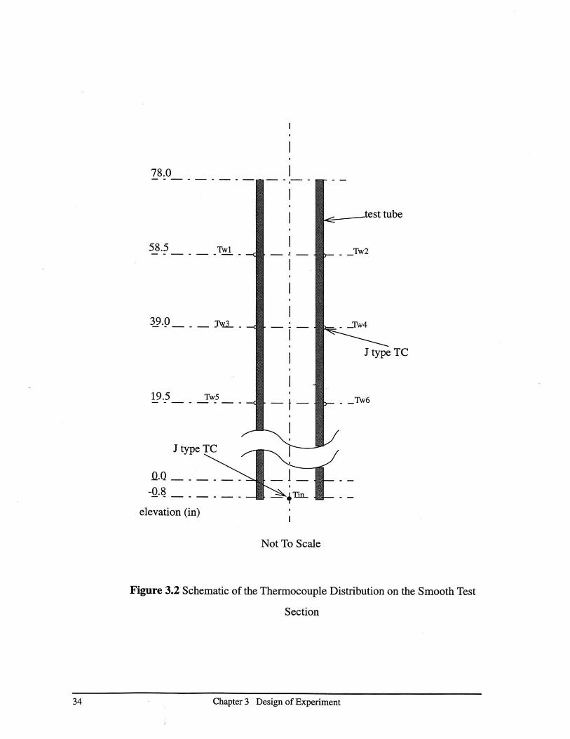
Seven stainless steel sheathed 1/16 inch O.D. thermocouples are mounted on the test

section as shown in Figure 3.2. Tw l-Tw6 are sandwiched between the tube wall and small

square pieces of 1/32 inch thick copper sheet. Thermocouple Tin is inserted into the test

tube at the inlet to make sure the coolant entering the test section is near saturation. A 16

channel thermocouple probe is vertically mounted inside the vessel to measure the axial

bulk temperature distribution of the atmosphere in the vessel at 6 inch axial intervals. Two

thermocouples are placed at the inlet of the downcomer and the outlet of the riser in the

separator to monitor the recirculation loop. All of these thermocouples are J-type.

One precise pressure transducer(0--100 psig) is installed to measure the vessel overall

pressure. One highly accurate differential pressure transducer is mounted at the bottom of

the separator to measure the pressure head induced by the water in the separator, thus the

water level. Two pressure gauges are also installed on the vessel and the separator to mon-

itor pressures visually.

One variable-area flowmeter is vertically mounted on the water and gas supply rig to

measure the volume flowrate of separator makeup water. A rotameter with mixing cham-

ber is used to measure the volume flowrates of air and helium as well as generating well-

mixed air/helium gas.

3.2.3 Data Acquisition System

A communication-based Data Acquisition System (DAS) was set up for this experiment as

shown in Figure 3.3. All thermocouple leads and pressure transducer output cables are

wired into the HP4471 1A multiplexer, which performs measurement channel selection.

The selected channel is then connected to a HP44702A Voltmeter to be sampled and con-


verted to digital signal, which then is transmitted to a PC via HP-IB serial communication

protocol. All of the above operations are programmable and command-driven, managed

by the HP3852A Data Acquisition and Control Unit.

A program, DATACQ.BAS, has been written to set up the user interface and communi-

cate with the HP3852A on the PC side in HP-BASIC and Assembly languages. The source

code is supplied in the floppy disk left in the possession of the NED Computer Facility

Administrator (see Appendix F).

3.2 Experimental Apparatus 33


78.0

58.5 Tw

39.0 TO-3\LL

19.5 Tw5

____________ I ____________ __

I -

-I-.

J type TC

.-. test tube

Tw2

- Iw4

J type TC

-TW6

1<-0.8

elevation (in)

Not To Scale

Figure 3.2 Schematic of the Thermocouple Distribution on the Smooth Test

Section


I


ThermocoupleLeads

0 0 0

Pressure TransducerOutput Cables

HP44711A High-speed Multiplexer

HP44702A High-speed Voltmeter

HP3852A Data Acquisitionand Control Unit

HP-IB Cable

Figure 3.3 Schematic of Data Acquisition System


PC with HP-IBProgramming Interface

I T v


3.3 Operation Procedure

3.3.1 Calibration of Measurement Devices

All thermocouples, pressure transducers and the variable-area flowmeter have been

already calibrated before delivery by the manufacturers.

The conversion factor from pressure drop rate in the separator to steam mass flow rate

is calculated and calibrated using the d.p. cell, the variable-area flowmeter and a digital

timer. The detailed procedure is described in Appendix G.

3.3.2 Adjustment of Operating Conditions

The major parameters to be adjusted during experiment operations are overall vessel pres-

sure and air mass fraction. The power supply automatically adjusts to follow the heat

transfer rate.

A Proportional-Integral-Derivative controller taking the temperature reading of the

water in the vessel as feedback was used to keep a stable temperature in the pressure ves-

sel, thus indirectly controlling the vessel pressure since the steam/gas mixture in the vessel

is in saturation status (at steady state). The desired temperature can be directly set on the

temperature controller panel. Thus the desired overall vessel pressure can be set by setting

the corresponding saturation temperature on the temperature controller panel.

The air mass fraction is adjusted by injecting the desired amount of air into the vessel.

The pressure change between before and after air injection is a good measure of the

amount of added air using the ideal gas law.

To make operation condition transitions, the following two steps are recommended:

1). Open the normal release valve to vent a certain amount of steam/air mixture if it is

desired to reduce air mass fraction since the steam loss will be compensated by evaporat-

ing more water in the vessel. Open the gas injection valve to inject a certain amount of air

if it is desired to increase air mass fraction.

2). Keep the temperature setting untouched and wait for the system to reach steady

state if no pressure change is desired. Change the temperature setting to the desired value

and wait for the system to reach steady state if a pressure change is desired. It usually

Chapter 3 Design of Experiment36

takes 30 minutes for the whole system to reach the new steady state after a condition

adjustment.

A Standard Operation Procedure for operating the experiment facility is attached in

Appendix H.

3.3.3 Data Collection and Processing

All data collection can be done automatically at a constant sampling interval (usually 2

minutes) except the d.p. cell output for the separator liquid level, which has to be visually

read from a readout device specially configured for this d.p. cell.

Before starting data collection, instrumentation and DAS checks have to be done.

Then start the PC side application DATACQ.BAS and follow the prompted instructions.

Data reduction and error analysis are described in Appendix G.

3.4 SummaryIn this chapter, design strategy and apparatus setup of the experiment are described. The

most notable things in the design are that the coolant is under boiling condition during

steady state and heat transfer rate is measured based on the steam generation rate in the

test section determined by measuring the rate of decrease in separator liquid inventory.

The Instrumentation and Data Acquisition system and operation procedure are also

described in the chapter.

3.4 Summary 37

3.4 Summary 37

Chapter 4

Results and Discussion for Smooth Tube

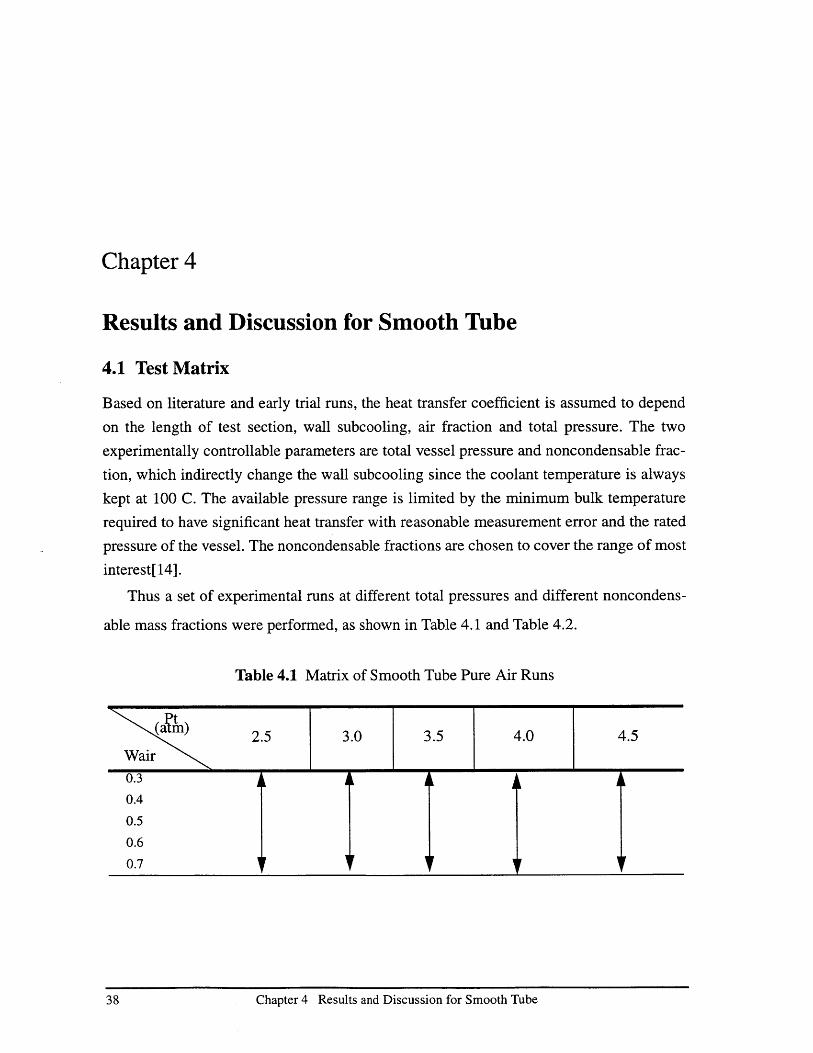
4.1 Test Matrix

Based on literature and early trial runs, the heat transfer coefficient is assumed to depend

on the length of test section, wall subcooling, air fraction and total pressure. The two

experimentally controllable parameters are total vessel pressure and noncondensable frac-

tion, which indirectly change the wall subcooling since the coolant temperature is always

kept at 100 C. The available pressure range is limited by the minimum bulk temperature

required to have significant heat transfer with reasonable measurement error and the rated

pressure of the vessel. The noncondensable fractions are chosen to cover the range of most

interest[ 14].

Thus a set of experimental runs at different total pressures and different noncondens-

able mass fractions were performed, as shown in Table 4.1 and Table 4.2.

Table 4.1 Matrix of Smooth Tube Pure Air Runs

m) 2.5 3.0 3.5 4.0 4.5Wair0.3

0.4

0.5

0.6

0.7

Chapter 4 Results and Discussion for Smooth Tube38

Table 4.2 Matrix of Smooth Tube Air-Helium Runs

Xs/(Xs+Xnc) 0.4 0.60.8

Pt(atm)Xhe/Xnc

15% 3.5,4.5 3.5,4.5 3.5,4.530% 3.5,4.5 2.5,3.0,3.5,4.0,4.5 3.5,4.560% 3.0

4.2 Repeatability of Experiments

To verify the reliability of data points and repeatability of the experiments, a complete

series of repeat runs at Pt=3.5 atm for the air-only case was conducted several weeks after

the initial run. As shown in Figure 4.14 the original points and repeat points are in good

agreement since their error bars overlap.

4.3 Condensation in the Presence of Air Only

4.3.1 Empirical Correlation from Experimental Data

An empirical heat transfer correlation of condensation in the presence of air has been

developed for a copper tube with length of 2 meters and O.D. of 4 cm in terms of a param-

eter group made up of steam mole fraction (Xs), overall pressure (P), temperature differ-

ence between bulk gas and wall surface (dT), which has taken into account all well-known

factors influencing condensation rate. A similar approach has been applied in the past by

others: for example Dehbi [1], Almenas [25]. Using all experimental data for pure air runs

and least square error criteria, the average heat transfer coefficient correlation takes the

form:

h = C x Xs2.344 X PtO.252 x dT.3074.1)

4.2 Repeatability of Experiments 39

4.2 Repeatability of Experiments 39

where,

h: average condensation heat transfer coefficient, w/(mA2*C)

C: constant coefficient, equals 1015.7

Xs: steam mole fraction, dimensionless

Pt: overall pressure, atm

dT: wall subcooling, Celsius degrees,

which has been obtained for:

2.5 atm < Pt < 4.5 atm

4 C < dT < 25 C

0.395 < Xs < 0.873

Figure 4.1 shows the comparison of experimental data points to the correlation. As can

be seen from this figure, this correlation covers all data points within 20%. Most points are

within +/- 15%.

4.3.2 Comparison of the Experimental Data to Theoretical Analysis

The condensation process in the presence of air is governed by two physical phenomena:

natural convection and gas diffusion. The experimental data will be compared against the

analysis results based on natural convection, equimolal counterdiffusion and diffusion

through stationary gas layer.

Natural Convection

Pure natural convection analysis [22] indicates that the average heat transfer coeffi-

cient h takes the form:

h~-K gpp2 Pr) 1/3 dT1/3 (4.2)


For the present experiment there is not significant temperature dependence of these

variables and the only variable that has important pressure dependence is density p. Using

the ideal gas law gives:

p -Pt (4.3)

Eventually we get

and

h-Pt2/3 dT11 3

Q -Pt2/3dT4/3

(4.4)

(4.5)

Equimolal Counterdiffusion

Assuming that the diffusion coefficient D is constant and the ideal gas law holds, anal-

ysis of equimolal counterdiffusion in a binary gas mixture for the steady, one-dimensional

case [26] shows that the diffusion rate is proportional to

bulk - Pswald)(4.6)

Where D is the diffusion coefficient, and Ps is the steam partial pressure. Because the dif-

fusion coefficient has the following temperature and pressure dependency [22]:

4.3 Condensation in the Presence of Air Only 41

D T1.632(4 7

the mass diffusion rate, thus the heat transfer rate has the following expression:

T (O.632 Psbulk - PS wall(

Pt (4.8)

where Pt is the overall pressure.

Diffusion through Stationary Gas Layer

Under the same assumptions as in equimolal counterdiffusion and assuming that the

diffusion process is at constant total pressure and temperature and the noncondensable gas

is stationary, analysis [26] shows that the mass diffusion rate, thus the total heat transfer

rate obeys the following expression:

) DPt 'Pt - Psbulk(

T Pt - PS (49)

Considering Eq. 4.7, we have

Q TO.632LnP t)bulk (4.10)Pt-Pswal

Figures 4.2 through 4.4 show the correlations of the experimental data based on the

above theoretical analyses. As is evident, equimolal counterdiffusion has the best fit. The

other two show widely scattered points. Thus we can conclude that the mass counterdiffu-

sion of steam and noncondensables plays the dominant role in the condensation process


that we are studying even though we can not simply use it to completely explain the entire

process, which also involves axial flow.

4.3.3 Comparison of the Experimental Data to Existing Correlations and Models

A number of correlations for condensation on a vertical wall in the presence of air have

been developed, most notably Uchida's empirical correlation, Peterson's Diffusion Layer

Model (DLM) and Dehbi's correlation. In this section we will compare our experimental

data to these correlations. A conservative curvature enhancement factor of 0.8 has been

applied to make our experimental data on a vertically mounted cylindrical tube with O.D.

of 4 cm comparable to correlations for condensation on a vertical wall, as suggested in [1].

Figure 4.5 shows that the DLM with suction factor predicts the data very well. Most of

the experimental data fall into the +/- 20% range of its prediction. Furthermore the DLM is

conservative for lower heat transfer coefficient cases, which are of our special interest.

Figure 4.6 shows that without considering the suction factor, the DLM underestimates h

significantly, especially at high h cases. Thus the suction factor is important in the conden-

sation process with high h since it involves a high mass transfer rate, the cause of suction.

Figure 4.7 shows that using least square error criteria, the experimental data are well

distributed around the 2.2 times h line from Uchida's correlation, which comes from a

least square fit of experimental data. It also shows that Uchida's correlation is conserva-

tive.

Figure 4.8 compares the DLM and 2.2 times hUchida correlations. As can be seen, the

DLM is in very good agreement with the much simpler Uchida correlation. This allows us

to use 2 .2 *hUchida to evaluate the performance of condensation on containments without

conducting complicated numerical computations as required by the DLM. However

Uchida's correlation tends to overpredict when the initial noncondensable gas pressure is

less than 1 atm or the noncondensable gas is not air. Thus caution should be used when

applying the 2 .2 *hUchida formula.

Since Dehbi has conducted experiments and developed a correlation under similar

working conditions, a comparison has been made as shown in Figure 4.9. As seen from

4.3 Condensation in the Presence of Air Only 43

this figure, Dehbi's correlation is conservative at high h cases. However, overall Dehbi's

correlation does not give a good prediction of our data.

4.4 Condensation in the Presence of Air and Helium

Following a loss of coolant accident (LOCA), hot steam will be injected into the contain-

ment building where it mixes with the air initially present. When the forced flow condi-

tions disappear, natural circulation currents become the driving mechanism allowing

steam to condense on colder containment walls. This heat transfer mode was the focus of

the experiments of section 4.2. If, for some reason, the reactor core is not adequately

cooled, the cladding may eventually oxidize and cause the release of hydrogen into the

containment. The purpose of this set of experiments is to study the effect of helium on

steam condensation. In these experiments, helium was substituted for hydrogen because of

many similarities between the two gases. Moreover, it is experimentally very demanding

to handle hydrogen because of its potential for combustion.

The range of physical parameters was chosen to correspond to typical values expected

in post LOCA conditions. The test matrix is shown in Table 4.2.

Figure 4.10 and Figure 4.11 show the effect of helium on condensation heat transfer at

total pressures of 3.5 and 4.5 atm, Xs values from 0.4 to 0.7, and helium mole fraction in

the air-helium mixture from 15% to 60%. As can seen from Figure 4.10 there is only a

small difference for Pt=3.5 atm between air-only cases and air-helium mixture cases when

Xhe/Xnc is less than 30%, which is of our major interest because it covers all conditions

experienced during a Severe Accident Scenario [14]. Figure 4.11 shows that while there is

a generally lower heat transfer coefficient for Pt=4.5 atm when the helium mole fraction

increases in the air-helium mixture, the difference is within 20% for the helium range of

less than 30%. Thus it is suggested that one utilize the air-only correlation with a reduction

factor of 20% to be conservative in the air/helium case as long as the total pressure is less

than 4.5 atm and Xhe/Xnc is less than 30%, since the helium effect increases with total

pressure, as shown in Figure 4.12. For applications beyond this range, it is suggested to


use the DLM [20] when implementation of complicate numerical computation procedure

and computation time are not of major concern, or Dehbi's correlation [1] for ease of use.

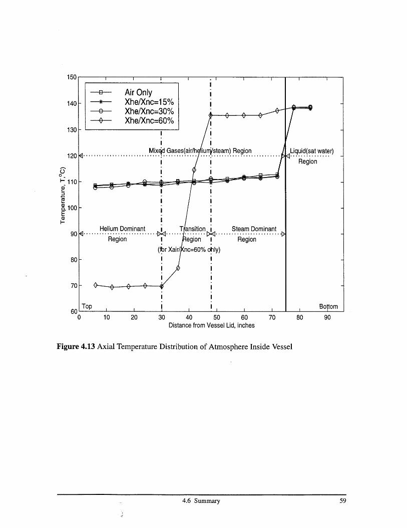
For helium mole fraction in excess of 60%, a gas stratification phenomenon was

clearly observed when steady state was reached, as shown in Figure 4.13,even though the

gases were initially well mixed. Also, unstable circulation occurred under this condition

because of the large axial temperature difference.

4.5 Shadowing Effect in a Tube Bundle

To evaluate a maximum upper limit for the shadowing effect in a tube bundle, a PVC

pipe shroud with I.D. of 10 cm and length of 2 m was added around the same smooth tube

used earlier to confine bulk gas flow entirely to the axial direction in an annular gap of

width 3 cm. The test matrix is shown in Table 4.3

Table 4.3 Matrix of Runs for Smooth Tube with Shroud

(an)2.5 3.0 3.5 4.0 4.5

Wair

0.35 X

0.42 X

0.52 X X X X X

0.62 X

Figure 4.15 shows the shroud effect versus air mass fraction at a constant total pressure

of 3.5 atm abs. Figure 4.16 shows that shroud effect versus total pressure at a constant air

mass fraction of approximately 0.52. It can be found from these two figures that heat

transfer coefficients are reduced by a factor of around 0.6 for tubes shadowed such that

only axial flow is allowed, compared to tubes in which unrestricted radial access is avail-

able. The magnitude is plausible because water vapor concentration in the downflowing

4.5 Shadowing Effect in a Tube Bundle 454.5 Shadowing Effect in a Tube Bundle 45

vessel atmosphere will become depleted when one proceeds from top to bottom of the

evaporator tube.

4.6 SummaryIn this chapter, the experimental results and comparisons to other empirical correlations

and theoretical models are presented.

First, it was found that the mass counterdiffusion of steam and noncondensables plays

the dominant role in the condensation process.

The DLM shows good agreement with the experimental data and thus is recommended

for use in containment analysis. Also 2.2* hUchida is recommended for engineering

design and analysis for its simplicity and ease of implementation with good agreement

with the experimental data and DLM prediction.

The effects of helium and bundle shadowing have been observed in the experimental

results. Reduction factors of 0.8 and 0.6 respectively have been recommended to predict

the performance of a smooth tube under influence of these effects.


35001

+ P=2.5 atmx P=3.0 atm

3000- 0 P=3.5 atm* P=4.0 atmo P=4.5 atm

0 2500 - h=1 01 5.7*Xs 2. 344 P 0.252*dTO. 307

+ 2000 - +0

00 1-;20-1-

500 - 0|0,

0

0 0. 15202.

-. 1500-

Em irca Paa e 4rGoP ,X .3 , .2 *d .37 .2 *C.7

Fi-af

5) 00

0 0.5 11.5 2 2.5

Empirical Parameter Group, XS2.34*pO252*dTO.3 07 atm .52CO.

Figure 4.1 Empirical Correlation of Air Noncondensable Runs for Smooth Tube

4.6 Summary 47

4.6 Summary 47

x

+ x

+

x 0

+x

0

+

0

,0

*

*

0

*

01

xO0

x

0

0

*

' I I I I I2.5 3 3.5

Parameter Group, Ln(Pt-.*dT)4 4.5

Correlation of Vertical Wall Data Reduced From Air Noncondensable Runs forSmooth Tube Based on Pure Natural Convection Model

Chapter 4 Results and Discussion for Smooth Tube

2.5

2

+ P=2.5 atmx P=3.0 atmo P=3.5 atm* P=4.0 atmo P=4.5 atm

1.5

1

0.5 H

6-C-J

C

a)E

CL

xwi

0

-0.5 H

+-1'1

1 . 2

Figure 4.2

5

48

8 10

Parameter Group,

12

Tv. 632*(dPs/Pt)

14 16 18

Correlation of Vertical Wall Data Reduced From Air Noncondensable Runs forSmooth Tube Based on Equimolal Counterdiffusion Model

4.6 Summary 49

12

10kH

I-

CESa)

a

EC)xw

+ P=2.5 atmx P=3.0 atmo P=3.5 atm* P=4.0 atmo P=4.5 atm

a) x

a)+2-

0-2

Figure 4.3

4 6

49

-

4.6 Summary

12

10- 0 P=3.5 atm* P=4.0 atmT P=4.5 atm

U) -

6d - -

c4-E

x (

*

0 1 1

-60 -50 -40 -30 -20 -10 0Parameter Group, Tv. 632 *ln((Pt-Pb)/(Pt-Pw))

Figure 4.4 Correlation of Vertical Wall Data Reduced From Air Noncondensable Runs forSmooth Tube Based on Diffusion through Stationary Gas Layer Model


-r-=x P=

flr.O Will

3.0 atm

50

1000 1500 2000h DLM With Suction, w/(m2*OC)

Figure 4.5 Comparison of Vertical Wall Data Reduced from Airfor Smooth Tube against DLM with Suction

Noncondensable Runs

4.6 Summary 51

+ P=2.5 atmx P=3.0 atmo P=3.5 atm* P=4.0 atmn P=-A rtm

4000

3500 F

0

S3000

x

c25000)

Q)

0

2000

cu 1500a)I

Ca)E 1000C)xwj

500

00

- - ..Yh =hexp DLM (With Suction) -

+20%'

--20%

.. I , - ' -I

500 2500 3000

514.6 Summary

4000 I I I

+ P=2.5 atm

3500- x P=3.0 atm0 P=3.5 atm* P=4.0 atm

E3000- o P=4.5 atmh =h

exp DLM (Without Suction)

+20%'2500 -

0 O

200000

'1500 ---0-20%

E 1000-

LU

500-

00 500 1000 1500 2000 2500 3000

h DLM Without Suction, w/(m2*OC)

Figure 4.6 Comparison of Vertical Wall Data Reduced from Air Noncondensable Runsfor Smooth Tube against DLM without Suction


4000

52

4500

+ P=2.5 atm4000- x P=3.0 atm

o P=3.5 atm .0i* P=4.0 atmE 3500 P=4.5 atm

- h =2.2*hUc

-3000 . ....... h eexp Uchida+20%

2500 - -0 0.

2000 -

cu

10 - 0' -20%

50 -..- ) -

Z0 15001

1000-.x Vw

0 500 h Uhida' w/(m2*oC) 1000 1500

Figure 4.7 Comparison of Vertical Wall Data Reduced from Air Noncondensable Runsfor Smooth Tube against Uchida Correlation

4.6 Summary 53

4.6 Summary 53

4000 1 1

+ P=2.5 atm

3500 x P=3.0 atmE 0 P=3.5 atm

* P=4.0 atm0 -o P = 4 .5 *.L3000 hDLM=12*h

-z DLM- Uchida

+20%'2500 --

2000 --

E - -0

c 1500 -.- 20%

0

00 500 1000 1500 2000 2500 3000

2.2*h ,cia w/(m2 C)

Figure 4.8 Comparison of DLM (With Suction) against 2.2*Uchida Correlation


1500hDehbi' w/(m2 OC)

Figure 4.9 Comparison of Vertical Wall Data Reduced from Airfor Smooth Tube against Dehbi Correlation

Noncondensable Runs

4.6 Summary 55

4000

3500

0

E3000

x

2500

0

2000

C

C-

*5 1500

E 1000

axw500

00

+ P=2.5 atmx P=3.0 atmo P=3.5 atm* P=4.0 atm0 P=4.5 atm

h =hexp Dehbi

+20%'

-20%

. .

- -- ---

500 1000 2000 2500 3000

4.6 Summary 55

0.4 0.45 0.5 0.55Xsteam, dimensionless

0.6 0.65 0.7 0.75

Figure 4.10 Helium Effect on Heat Transfer Coefficient at Pt=3.5 atm


2000

1800

C

0

0

1600-

1400-

1200-

1000-

800-

600 -

400-

200-

-- +- Air Only--- -x - Xhe/Xnc=1 5% ;- -e - Xhe/Xnc=30%

/ /

I I I I I I I II-

0.35

56

0.4 0.45 0.5 0.55 0.6 0.65Xsteam, dimensionless

0.7 0.75

Figure 4.11 Helium Effect on Heat Transfer Coefficient at Pt=4.5 atm

4.6 Summary 57

2000

1800 -

1600 -

0

C:

t

U)

00

-- *- Air Only- -*- Xhe/Xnc=1 5%- -8- Xhe/Xnc=30%

A/

/ / / 7

/ / -

--

lo,7 -

7 -

7 -oe

Ile

ol 11 -

I I I I I I I

1400-

1200-

1000-

800-

600

400

2000.3I5

4.6 Summary 57

1200

1100 F

1000

900)-

800 H

700 H

600 F

5002 2.5 3 3.5

Total Pressure, P, atm4 4.5

Figure 4.12 Helium Effect on Heat Transfer Coefficient at Xsteam=0.61


j0

-C"

CU)0

000U)C,,C

H

U)I

-- *- Air Only- -x - Xhe/Xnc=30%

I

//

/

//t"'-t'-''

/ /

/ //1/

I'

5

58

* I150 -

140-

130-

e Xhe/Xnc=30%0 Xhe/Xnc=60%

MiXE d Gases(air/h iurqsteam) Region

Helium Dominant T ansition .. Steam Dominant

Region I egion I Region

(br Xair nc=60% ohly)

0 10 20 30 40 50 60 70 80 90Distance from Vessel Lid, inches

Figure 4.13 Axial Temperature Distribution of Atmosphere Inside Vessel

4.6 Summary 59

9 Air Only* Xhe/Xnc=15%

Liquid(sat water)

Region

I Boltom

120 1- -

10-

00 -

F1

E

90 4

801

701-

Top60

i

I

4.6 Summary 59

0.3 0.35 0.4Air Mass Fraction,

0.45 0.5Wair, dimensionless

0.55 0.6

Figure 4.14 Repeatability of Smooth Tube Air-only Experiment Data at Pt=3 atm


'3000

2500

-* Initial Run-o- - Repeat Run

.

a)0

a)0

a)U)

2000 F

1500 F

1000-

500

0.0.2 0.25 0.65

60

1400

1200

1000

800

600

400

2000. 0.6 0.65

Figure 4.15 Shroud Effect on Heat Transfer Coefficient at Pt=3.5 atm

4.6 Summary 61

2000

1800

1600

0

(D

7,

-- *+- Without Shroud-x - With Shroud

NN

N N

- N

- -

NNNN N- -

-N N

- -- -

0.4 0.45 0.5 0.55Air Mass Fraction, Wair, dimensionless

3 0.35 0.7

4.6 Summary 61

1200

1000-

8001-

600 F

4001-

200 -

02 2.5 3.5

Total Pressure, P, atm

Figure 4.16 Shroud Effect on Heat Transfer Coefficient at Wair=0.52


C

(D0

C/)C

- I iho tS ru -

- -x*- Withou ShroudT

- - --

3 4 4.5 5

62

Chapter 5

Results and Discussion for Finned Tubes

5.1 Introduction

Augmentation of heat transfer and reduction of the coolant pumping power consumption

by devices in which heat transfer occurs are the twin goals in improving the design of heat

transfer equipment. The achievement of the enhancement of heat transfer is of particular

importance in the PCCS concept design since the driving head of the coolant is provided

by natural circulation. Only increase of heat transfer surface is considered for enhance-

ment means since it is hard to increase heat transfer coefficient because of the existence of

a large amount of noncondensable gases.

Major parameters governing the performance of a evaporator made up of finned tubes

are the length and diameter of the tube, the fin geometry and the number of tubes. To find

the optimal finned surface for given heat exchanger applications, it is necessary to estimate

the fin effectiveness and the cost of manufacture. Two standard and widely-used shapes,

round radial-fin and straight axial-fin were investigated in our design since they are rela-

tively easy to make and have low cost resulting from their extensive applications in a num-

ber of industries. The theoretical design and experimental tests are discussed in the next

sections.

5.2 Finned Tube Parametric Design Based on Theoretical Analysis

Finned tube heat transfer is a one-dimensional heat conduction problem in general. The

mathematical analysis for finned tubes is based upon the assumptions listed in Section

5.1 Introduction 63

5.1 Introduction 63

2.2.1.

5.2.1 Radial-finned Tube

The governing equation of this problem is:

d2 1 d 2h (5.1)

dr2 rdr X8

where,

r is the radial coordinate with origin at the center of the tube cross section.

0 is the temperature difference between the surface at r and the surrounding fluid.

h is the average heat transfer coefficient on the surface of fin.

X is the thermal conductivity of fin material

8 is the thickness of the fin.

The boundary conditions for the above equation are:

0| r=Rb Ob (5.2)

d (5.3)

dr r = Rout

Solving the above equation with the given B.C.s gives the fin efficiency $ (for one fin),

defined as:

f Jf OdA (54)

ObAf

in the form [21]:

Chapter 5 Results and Discussion for Finned Tubes64

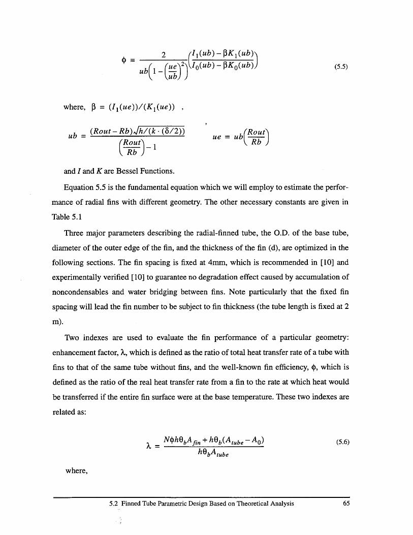
2 (1,(ub) - KI(ub)

ub 1- ()2)YIO(ub) - PKO(ub)) (5.5)ub

where, P = (I(ue))/(KI(ue))

ub = (Rout - Rb)h/(k (8/2)) ue = ub RoutRout Rb

Rb

and I and K are Bessel Functions.

Equation 5.5 is the fundamental equation which we will employ to estimate the perfor-

mance of radial fins with different geometry. The other necessary constants are given in

Table 5.1

Three major parameters describing the radial-finned tube, the O.D. of the base tube,

diameter of the outer edge of the fin, and the thickness of the fin (d), are optimized in the

following sections. The fin spacing is fixed at 4mm, which is recommended in [10] and

experimentally verified [10] to guarantee no degradation effect caused by accumulation of

noncondensables and water bridging between fins. Note particularly that the fixed fin

spacing will lead the fin number to be subject to fin thickness (the tube length is fixed at 2

m).

Two indexes are used to evaluate the fin performance of a particular geometry:

enhancement factor, X, which is defined as the ratio of total heat transfer rate of a tube with

fins to that of the same tube without fins, and the well-known fin efficiency, $, which is

defined as the ratio of the real heat transfer rate from a fin to the rate at which heat would

be transferred if the entire fin surface were at the base temperature. These two indexes are

related as:

NohObAfif + hOb(A tube - A ) (5.6)hobAtube

where,

5.2 Finned Tube Parametric Design Based on Theoretical Analysis 65

AO is the tube surface covered by fins,

Afi, is the surface area of fins,

Atibe is the total surface of the smooth base tube,

N is the number of fins.

The O.D. of the base tube was selected as 4 cm (around 1.59 inches) because this is

one of the most regular sizes commercially available, which can reduce the cost of heat

exchangers consisting of hundreds of tubes of this type. Also it is large enough to provide

a reasonably small flow friction.

Figure 5.1 and Figure 5.2 show how the enhancement factor and fin efficiency vary for

different fin thickness and radius of fin outer edge. The strategy is that we want to have a

high enhancement factor since it is directly related to the performance of our cooling unit,

a reasonably high fin efficiency and low cost and size of the finned tube. Figure 5.1 shows

that the enhancement factor is not sensitive to fin thickness when it is greater than 2 mm.

Figure 5.2 shows that greater thickness yields higher fin efficiency. Thus we selected fin

thickness at 3 mm since it has a fin efficiency of 0.56 and the weight of the finned tube,

thus cost, still acceptable. The selection of the radius of the fin outer edge is mainly based

on the consideration of size. Eventually we selected a radius of 5 cm because of the size

consideration, plus the enhancement factor increases very slow when the radius increases

beyond 5 cm as demonstrated in Figure 5.1.

Consequently, a copper-radial-finned copper tube with features described in Table 5.2

is proposed to serve in the evaporator of the PCCS concept. The schematic of the proposed

tube is sketched in Figure 5.5.


Table 5.1 The Constants Used in Estimating the Performance of the Finned Tubes

Items Values

The tube length 2m

The fin spacing 4 mm

The temperature between fin at 15C(120-105)base and surrounding fluid

Thermal conductivity of copper 400 w/(m*k)

Average heat transfer coefficient 1000 w/(mA2*k)

Table 5.2 Features of the Proposed Radial-finned Tube for the Evaporator

Items

Outer diameter of tube

Diameter of fin outer edge

Fin thickness

Fin spacing

tube length

Values

4 cm

10 cm

2 mm

4 mm

2 m


15

0

0

4J

0

ra.0

24.

0

101

5

0.03 0.04 0.05 0.06 0.07

Radius of Fin Outer Edge (m)

Fin Thicknesss=1 mmFin Thicknesss=2 mmFin Thicknesss=3 mmFin Thicknesss=4 mm

Figure 5.1 Radial-fin Enhancement Factor Changes with Geometry

0.03 0.04 0.05 0.06 0.07

Radius of Fin Outer Edge (m)

Fin Thicknesss=1 mmFin Thicknesss=2 mmFin Thicknesss=3 mmFin Thicknesss=4 mm

1

.2

~0

0

E0

0.5

0

Figure 5.2 Radial-fin Efficiency Changes with Geometry

Chapter 5 Results and Discussion for Finned Tubes

0.05

I I I0.I5

------ ---- -~ - - - -~ ~ ~ - 0.56

68

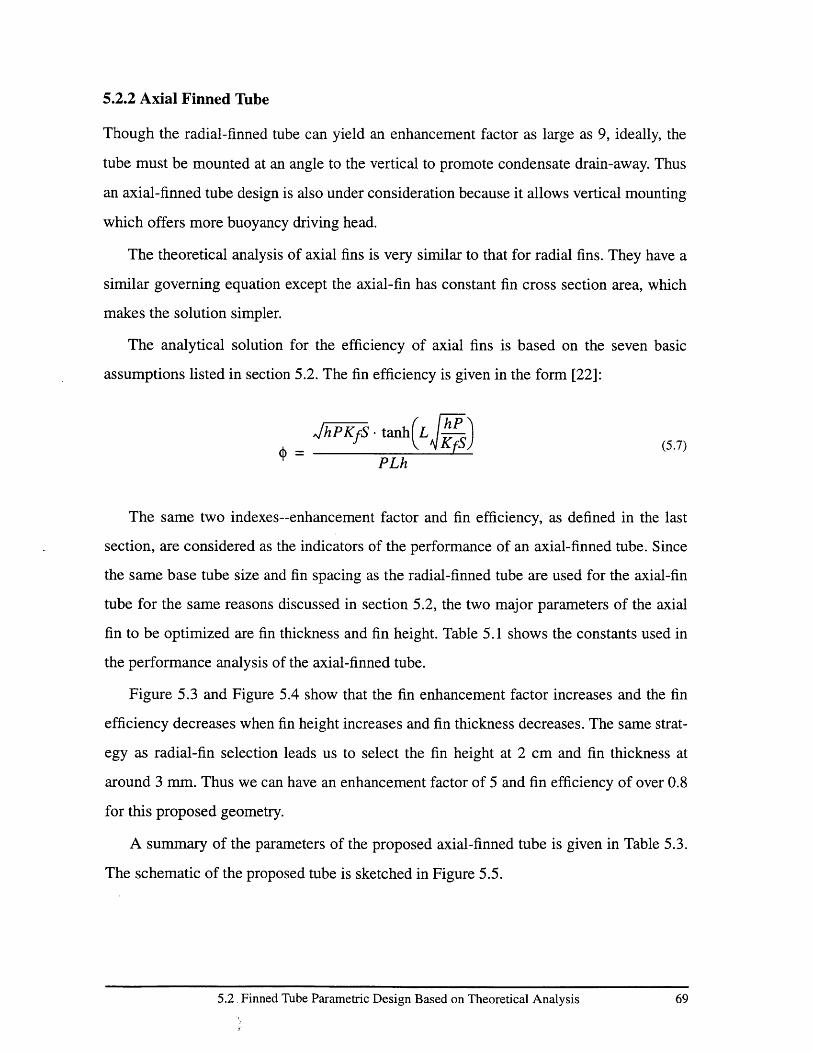
5.2.2 Axial Finned Tube

Though the radial-finned tube can yield an enhancement factor as large as 9, ideally, the

tube must be mounted at an angle to the vertical to promote condensate drain-away. Thus

an axial-finned tube design is also under consideration because it allows vertical mounting

which offers more buoyancy driving head.

The theoretical analysis of axial fins is very similar to that for radial fins. They have a

similar governing equation except the axial-fin has constant fin cross section area, which

makes the solution simpler.

The analytical solution for the efficiency of axial fins is based on the seven basic

assumptions listed in section 5.2. The fin efficiency is given in the form [22]:

hPKfS - tanh(L hP) (5.7)PLh

The same two indexes--enhancement factor and fin efficiency, as defined in the last

section, are considered as the indicators of the performance of an axial-finned tube. Since

the same base tube size and fin spacing as the radial-finned tube are used for the axial-fin

tube for the same reasons discussed in section 5.2, the two major parameters of the axial

fin to be optimized are fin thickness and fin height. Table 5.1 shows the constants used in

the performance analysis of the axial-finned tube.

Figure 5.3 and Figure 5.4 show that the fin enhancement factor increases and the fin

efficiency decreases when fin height increases and fin thickness decreases. The same strat-

egy as radial-fin selection leads us to select the fin height at 2 cm and fin thickness at

around 3 mm. Thus we can have an enhancement factor of 5 and fin efficiency of over 0.8

for this proposed geometry.

A summary of the parameters of the proposed axial-finned tube is given in Table 5.3.

The schematic of the proposed tube is sketched in Figure 5.5.


.2

I-

0

a20Ua0a

0 0.01 0.02 0.03Fin height (m)

Thickness=1.0 mmThickness=2.0 mmThickness=3.0 mmThickness=4.0 mmThickness=5.0 mm

Figure 5.3 Axial-fin Enhancement Factor Changes with Geometry

I

jaC

a

'aUaU

a

0.8

0.6

0.4

0.20 0.01 0.02 0.03

Fin height (m)

* Thickness=1.0 mmThickness=2.0 mmThickness=3.0 mmThickness=4.0 mmThickness=5.0 mm

Figure 5.4 Axial-fin Efficiency Changes with Geometry


I I I I

0.0 ...

I | | |

0.04 0.05

N~~2

~0.8

I X

0.04 0.05

70

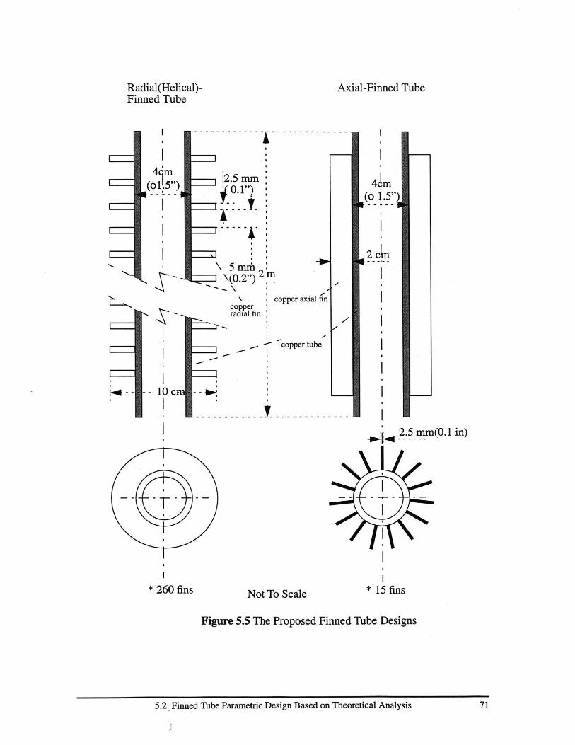
Radial(Helical)-Finned Tube

Axial-Finned Tube

4 m

($15") -' - - - I:2.5 mm] ' .1"7)

\ Smm21 \(0.2") 2 m

copper

10 -

* 260 fins

axial An

copper tube

Not To Scale

2.5 mm(O. 1 in)

* 15 fins

Figure 5.5 The Proposed Finned Tube Designs

5.2 Finned Tube Parametric Design Based on Theoretical Analysis

4Jm

2 c :

ra falrfin

71

Table 5.3 Features of the Proposed Axial-finned Tube for the Evaporator

Items Values

Outer diameter of base tube 4 cm

Length of the base tube 2 m

Fin height 2 cm

Fin thickness 3 mm

Fin spacing 4 mm

5.3 Results and Discussions of Finned Tubes Tests

Due to lack of commercial availability of the proposed finned tubes described in the pro-

ceeding section, an in-housemade copper-axial-finned copper tube and an aluminum-

radial-finned stainless steel tube manufactured by Hudson Product, which was originally

designed for forced air cooling units, were investigated. Their geometries are shown in

Figure 5.6 and Figure 5.7. The axial-finned tube geometry is as close as possible to the

design proposed in Table 5.3. The radial-finned tube has a smaller fin spacing than the

design proposed in Table 5.2

5.3.1 Axial-finned Tube

The performance of the tested axial-finned tube is shown in Figure 5.8 and Figure 9. An

enhancement factor of over 1.5 can be easily obtained while the analytical solution gives

an enhancement factor of around 4.5 assuming perfect contact of the fin and the base tube.

A number of reasons contribute to this difference. First of all, some of the assumptions on

which the analytical solution is based may not hold for the real case, for example, the heat

transfer coefficient is not uniform over the whole surface of the finned tube. The existence

of fins may retard noncondensable gas convection, thus reduce heat transfer rate. Also

because this axial-finned tube was fabricated in-house using soft-soldering techniques,

there is some uncertainty as to how well the gap between fin and base tube is filled

although there is no visual evidence of an unfilled gap. The analytical solutions for this


finned tube with all-air and all-solder gaps, assuming a gap of 0.2 mm, are shown in Fig-

ure 5.8 and Figure 5.9. The experimental data fall between these two extreme cases.

5.3.2 Radial-finned Tube

Figure 5.10 and Figure 5.11 show the performance of the radial-finned tube with

geometry shown in Figure 5.7, which was tilted 15 degrees from the vertical. Most of the

enhancement factors are between 1 and 1.5 while the analytical solution, assuming perfect

conditions as discussed in section 5.2, predicts enhancement factors of 4 to 6. Major rea-

sons for the degrading are the following:

1. This tube also has a contact thermal resistance problem: the radial fins are mechani-

cally pressed onto the base tube (the "radial" fins are actually helically wrapped on the

base tube).

2. The spacing of the fins (2.5 mm) is well below the recommended 4 mm in Ref [10],

which notes heat transfer degradation when fin spacing is less than 4 mm. Thus noncon-

densable build-up and water bridging would significantly reduce the heat transfer rate.

3. This tube was tested at 15 degrees from vertical rather than horizontal, a factor

which would increase the water bridging tendency. A test in the vertical position was car-

ried out and an "enhancement factor" less than 1.0 was measured.

5.4 SummaryIn this chapter optimized designs of an axial-finned tube and a radial-finned tube are pre-

sented. A made-in-house axial-finned tube and a commercial radial-finned tube, which

was originally designed for forced air cooling, have been tested under conditions similar

to the smooth tube. A summary of enhancement factors for the axial-finned tube and the

radial-finned tube is shown in Table 5.4. The reasons for degraded performance of these

finned tubes are discussed in this chapter. It has been pointed out that the nonuniform dis-

tribution of heat transfer coefficient and the contact thermal resistance at the fin root are

the primary reasons the finned tubes did not perform as predicted by theoretical analysis.

Too small fin pitch and tilting angle are other important reasons for the performance deg-

radation of the radial-finned tube.

5.4 Summary 73

5.4 Summary 73

Table 5.4 Summary of Enhancement Factors for Proposed and Tested Finned Tubes

Proposed Geometry Tested Geometry Tested Geometry(Analytical Results (Analytical Results (Experimental

for Ideal Case) for Ideal Case) Results)

Axial-finned Tube 5 4.4 1.6

Radial-finned Tube 9 7.9 1.2


1.98 m

43.2 cin

1.91 c n

4r a,

3.18 mm

i-/

Not to Scale

Material: Copper * 12 fins

Figure 5.6 Schematic of the Tested Axial-finned Tube

5.4 Summary 75

stag(lotv

cutto]

at 45 degree anglepromote drainage

ger mounted axiallywjr Ain is betweeno pper fins)

755.4 Summary

4JrnV

Lo

L mm.

2.5 ram

2m

Aluminunradial fin

-Aluminum Outer Tube

Stainless Steel Base Tube

--- --- c -T

~~~1~~~~ * 680 fins for 2 m

Note: Fins are actually helically wrapped

Not To Scale

Figure 5.7 Schematic of the Tested Radial-finned Tube


K

I:

~-, \

I

I

76

4.50

4

3.5

C0

c 3E

0q 2.5

U-C

Eu2

C

C

w1.5

0.52.5 3 3.5 4 4.5

Pt, atm

Figure 5.8 Enhancement Factors of the Axial-finned Tube at Wair=0.54

5.4 Summary 77

o ...........

Experimental Data-*+- All Air Gap--- All Solder Gap0. Perfect Contact

- --------- ------- *- ----------- ---- * ------ ------- -

I

5.4 Summary 77

5

45 0

2 .5 - -----.. .. .. ...--. .-.-.-. .- -. .- -.-- -- --.-- - -. .-- - -- - - -- -.-- -

0..

CO)E

E

0

U)

EC

- Experimental Data-*- All Air Gap

1.5 -.. -.. -. .-..-.-..-..-... ..- -o A ll S older G apPerfect Contact

---------------------------------0.5

0.45 0.5 0.55 0.6 0.65 0.7Wair, Dimensionless

Figure 5.9 Enhancement Factors of the Axial-finned Tube at Pt=4.5 atm


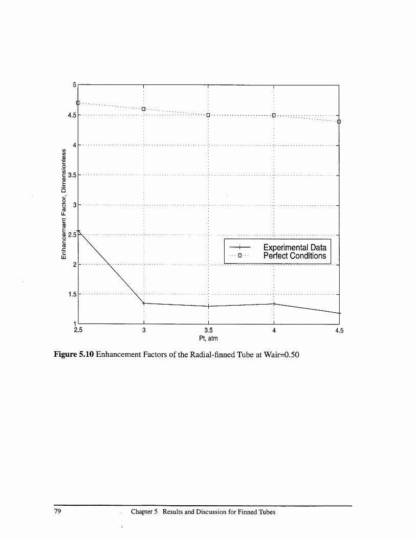
5

4.5

C0w'Cw)E0

(DE-

Ca

CCU

4

3.5

3

2.5

2

1.5

2.5 3 3.5Pt, atm

4

Figure 5.10 Enhancement Factors of the Radial-finned Tube at Wair=0.50


.. -- ---.- -.- -.-.- -- -- -- - -- -- ---.. . .

- . . . .. .. . ..-..-.-. .-.- -. .-.-- - ..-.- - - -------- - - -- -- - -- - - - - -

- -E

Experimental DataPerfect Conditions

-........................-.-.-.- -.-.-.-.-. .-.-. .-- --- --.-.- -.-- - -.- -. .- -.-.-.-- - --.--

-- -- -- ---- - - -- --- - -- -------- -- --- ---- - -- ---- ---------- ---- -- -.. ........

1'4.5

I I I

I

79

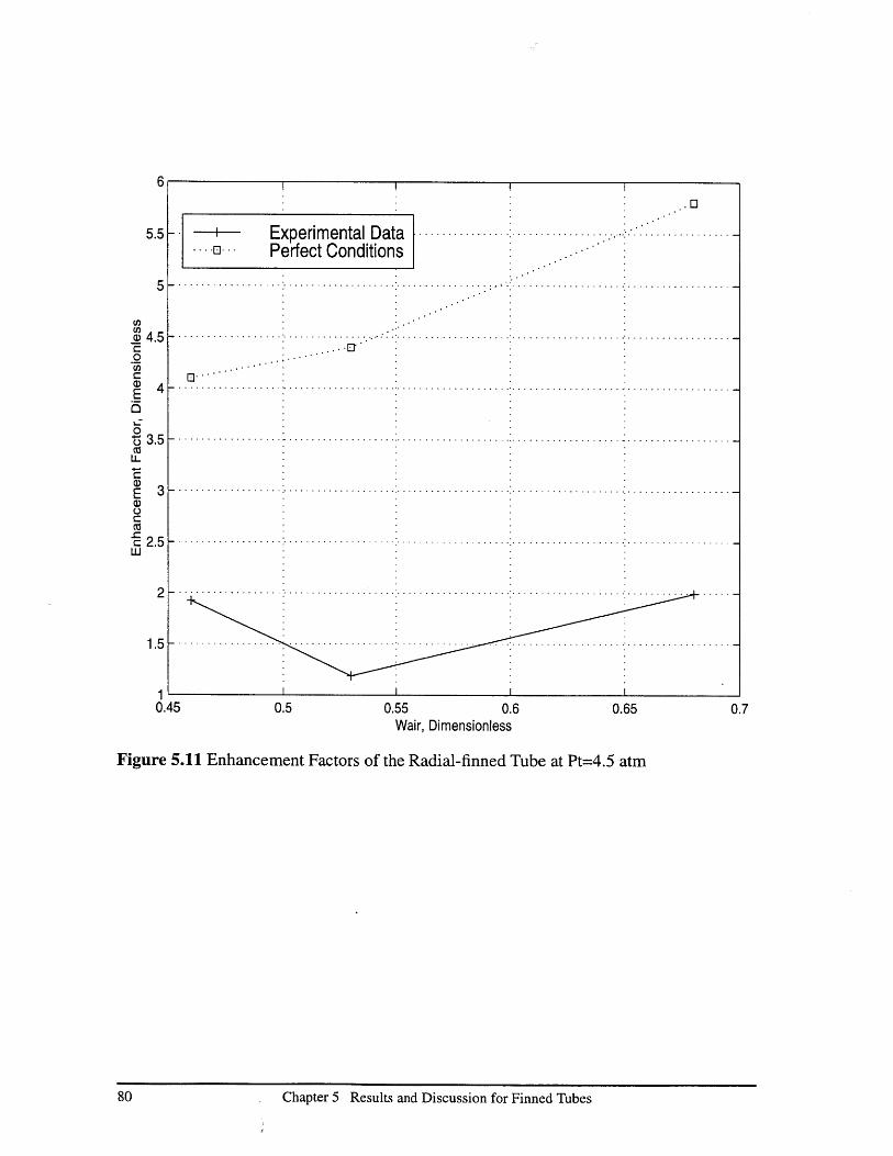
0.5 0.55 0.6Wair, Dimensionless

0.65 0.7

Figure 5.11 Enhancement Factors of the Radial-finned Tube at Pt=4.5 atm


6

5.5 I

5

Experimental Data- .. Perfect Conditions

................... . .

- . . . . .. . . .. . . . .. . . . ... .. . . . . .. ... . . . .. . . . . . .

---..--- ..- ..-.--- ..-.- ..-- .---- ..- ..-.- ...--- .-- ...-- ............. .. -.. -.. -..-..-

- - - - - - - - - - - - -- - - - - -- -- - ----.. ... ... .. ..... ... ... ... ..

4.5

4

(nCna)C0U)Ca)E

0

CU)

E(DC)

CzC

3.5

3

2.5

2

1.5

10.45

80

Chapter 6

Summary, Conclusions and Recommendations

6.1 Summary and Conclusions

Two conceptual PCCS designs: the thermosyphon loop and the IEO, are addressed and

their key features are presented in this thesis. Based on their requirements, a number of

full-scale single-tube experiments have been conducted to investigate the performance of

the evaporator, the key component in both PCCS designs. The referenced reports by

Leiendecker [13], Byun [14] and Mattingly [2] describe other efforts made at MIT on the

PCCS conceptual designs and contaminant analysis.

The past work on external filmwise condensation on vertically mounted smooth and

profiled surfaces in the presence of noncondensables has been reviewed with emphasis on

the DLM. Italian work on tilted radial-finned tube tests in the presence of noncondensable

is also referenced. Their recommended 4 mm for the fin spacing is adopted in our finned

tube design.

The design strategy and apparatus setup of the experiment are described in detail. Two

designs optimized to enhance heat transfer of an axial-finned tube and a radial-finned tube

are proposed. The smooth tube, as the reference, has been tested for total pressure ranging

from 36 psia to 66 psia, and air mass fraction ranging from 0.3 to 0.65, in the presence of

pure air and an air-helium mixture, respectively. The maximum shadowing effect in a tube

bundle was also tested by adding a cylindrical shroud around the smooth tube. A made-in-

house axial-finned tube and a commercial radial-finned tube, which was originally

Chapter 6 Summary, Conclusions and Recommendations81

designed for forced air cooling, have been tested under conditions similar to the smooth

tube.

Analysis of our experimental data and comparison to existing widely-used correlations

and models lead to the following conclusions:

1. The mass counterdiffusion of steam and noncondensables plays the dominant role in

the condensation process under our experimental conditions.

2. DLM with suction is recommended for use in containment analysis. Also 2.2*

h_Uchida is recommended for engineering design and analysis for its simplicity and ease

of implementation with good agreement with our experimental data and DLM prediction.

3. It is suggested that one utilizes the air-only correlation with a reduction factor of

20% to be conservative in the air/helium (simulating hydrogen) case as long as the total

pressure is less than 4.5 atm and Xhe/Xnc is less than 30%

4. A reduction factor of 0.6 is recommended for tube bundle shadowing effects until

more definitive work can be completed in this area.

5. A reduction factor of 0.5 is recommended to obtain the actual enhancement factors

of finned tubes from the predictions of theoretical models, again until further work demon-

strates otherwise.

6.2 Recommendations for Future Work

To improve the evaporator tube design and investigate its performance, the following tasks

are recommended for future execution:

1. Make in house another axial-finned tube according to the optimized design with bet-

ter fabrication techniques, e.g. using silver-soldering to replace soft-soldering to reduce

the thermal resistance of the solder.

2. Make in house a radial-finned tube by soldering "slotted-washers" with slightly

smaller I.D. than the tube O.D. on the base copper tube. The low enhancement factors

obtained for the tested radial-finned tube imply noncondensable gas is dominating the heat

transfer process. Much smaller fins may be almost as good.


3. Conduct all-steam runs for the smooth tube, proposed axial-finned tube and radial-

finned tube to eliminate the effect of noncondensables. Thus one will be able to evaluate

how much water bridging affects finned tube performance.

4. Increase the tilting degree of the radial-finned tube from 15 to 30 degrees from the

vertical to reduce water accumulation on fins.

5. Develop a new model starting with the DLM to better represent our experimental

data.

6. Run experiments for vertical cylinders at other diameters to evaluate the curvature

enhancement effect compared to a planar vertical wall.

7. Order another d.p. cell with 0-5 V voltage output for the separator pressure head

measurement to make it directly readable to the HP Data Acquisition and Control Unit.

Use a new up-to-date PC to integrate the current Data Acquisition System and data reduc-

tion process.

8. Investigate tube bundle effects by adding dummy tubes around the tested tube.

9. Design and investigate a pin-finned configuration since it improves the condensate

drainage and reduces noncondensable build-up.


References

[1] A. A. Dehbi, "The Effects of Noncondensable Gases on Steam Condensation underTurbulent Natural Convection Conditions", MIT Ph.D. Thesis in Department ofNuclear Engineering, 1991.

[2] B. Mattingly, "Containment Analysis Incorporating Boundary Layer Heat and MassTransfer Techniques", MIT Ph.D. Thesis in Department of Nuclear Engineering,1999.

[3] P. F. Peterson, "Theoretical Basis for the Uchida Correlation for Condensation inReactor Containments", Nucl. Eng. and Design 162 (1996).

[4] L. E. Herranz, M. H. Anderson, M. L. Corradini, "A Diffusion Layer Model for SteamCondensation within the AP600 Containment", Internal Report in Dept. of Nucl.Eng. and Eng. Physics in Univ. of Wisconsin.

[5] K. Huhtiniemi, M. L. Corradini, "Condensation in the Presence of NoncondensableGases", Nucl. Eng. and Design 141 (1993).

[6] S. L. Chen, F. M. Gerner, and C. L. Tien, "General Film Condensation Correlations",Experimental Heat Transfer, vol. 1, pp. 93-107, 1987.

[7] J. W. Rose, "Fundamentals of Condensation Heat Transfer: Laminar Film Condensa-tion", JSME Int'l Journal, Series II, Vol. 31, No. 3, 1988.

[8] V. Srinivasan, R. K. Shah, "Fin Efficiency of Extended Surfaces in Two-phase Flow",Int. J. Heat and Fluid Flow 18:419-429, 1997.

[9] Forsberg, C.W. et al. (1994) Use of Temperature-Initiated Passive Cooling System(TIPACS) for Modular High-Temperature Gas-Cooled Reactor Cavity Cooling sys-tem; Oak Ridge National Laboratory, ORNL-6767, Oak Ridge, Tennessee.

[10] Cavicchia V. and Vanini P. (1996) Innovative containment cooling for a double con-crete containment; Int. Conf. on Nuclear Engineering ICONE-4, ASME, Vol. 2.

[11] J. N. Castle, "Survey of the State of the Art in Mitigation Systems, NUREG/CR-3908, Chapter 5, 1988

[12] Ahmad, A. et al. (1983) PWR Severe accident delineation and assessment; NUREG/CR-2666; UCLA-ENG-8284

[13] M. Leiendecker, N. E. Todreas, M. J. Driscoll and A. Hurtado, "Design and Numeri-cal Simulation of a Two-Phase Thermosyphon Loop as a Passive ContainmentCooling System for PWRs", Volume I, MIT-ANP-TR-053, 1997.

[14] C. S. Byun, N. E. Todreas and M. J. Driscoll, "Conceptual Design and DistributedParameter Analysis of A Semi-passive Containment Cooling System for A LargeConcrete Containment", MIT-NFC-TR-017, Feb. 1999.

[15] H. Uchida, A. Oyama and Y. Togo, "Evaluation of Post-accident Cooling Systems ofLight-water Power Reactors", Proceedings of the Third International Conference onthe Peaceful Uses of Atomic Energy, Geneva, Aug. 31- Sept. 9, 1964, Vol. 13,United Nations, New York, 1965, pp. 93-104.

84

[16] T. Tagami, "Interim Report on safety assessments and Facilities EstablishmentProject for June 1965", No. 1, Japanese Atomic Energy Agency, 1965, unpublishedwork.

[17] R. G. Gido and A. Koestel, "Containment Condensing Heat Transfer", 2nd Int'l Top-ical Meeting on Nuclear Reactor Thermal Hydraulics (NURETH-2), 1983, pp 1111-1119.

[18] M. L. Corradini, "Turbulent Condensation on a Cold Wall in the Presence of a Non-condensable Gas", Nuclear Technology, Vol. 64, 1984, pp. 186-195.

[19] P. F. Peterson, V. E. Schrock and T. Kageyama, "Diffusion Layer Theory for Turbu-lent Vapor condensation with Noncondensable Gases", ASME Journal of HeatTransfer, Vol. 115, 1993, pp. 998-1003.

[20] M. H. Anderson, L. E. Herranz, M. L. Corradini, "Evaluation of Condensation Mod-eling Based on Mass Transfer Analogy", Proceedings of the 1997 National HeatTransfer Conference, Baltimore, August 1997.

[21] K. A. Gardner, "Efficiency of Extended Surfaces", ASME Journal of Heat Transfer,1944.

[22] A. F. Mills, "Heat and Mass Transfer", published by R. D. Irwin Inc., 1995.[23] J. P. Pearson and B. Gschwend, "PSI Nuclear Energy and Safety Research", PSI

Annual Report, Annex IV, 1997.[24] K. 0. Beatty and D. L. Katz, "Condensation of Vapors on Outside of Finned Tubes",

Chemical Engineering Progress", Vol. 44, No. 1, pp. 55-70, 1948.[25] K. Almenas, U. C. Lee, "A Statistical Evaluation of the Heat transfer data Obtained in

the HDR Containment Tests", Univ. of Maryland, Nuclear Engineering Depart-ment, 1985.

[26] W. M. Rohsenow and H. Y. Choi, "Heat, Mass, and Momentum Transfer", publishedby Prentice-Hall, Inc., New Jersey, 1963

[27] Bertela, M. and Prakash, J. (1988); Transport of thermal energy by simple two-phaseloop; Int. Journal of Energy Research, Vol. 12, pp. 679-698.

[28] Bodi, A. et al. (1996); Advanced containment concepts for light-water nuclear reac-tors; Massachusetts Institute of Technology, Internal Report.

[29] Cavicchia V. and Vanini P. (1996) Innovative containment cooling for a double con-crete containment; Int. Conf. on Nuclear Engineering ICONE-4, ASME, Vol. 2.

[30] Chen, K.S. and Chang, YR. (1983); Steady-state analysis of two-phase circulationloop; Int. Journal Heat and Mass Transfer, Vol. 31, No. 5, pp. 931-940.

[31] Deng, S-J. (1990); Heat transfer enhancement and energy conservation; HemispherePublishing Corporation, New York.

[32] Dunn, P.D. and Reay, D.A. (1982); Heat pipes; Pergamon Press, New York.[33] Erbacher, F.J. and Neitzel, H.J. (1992) Passive Containment cooling by natural air

convection for next generation Light Water Reactors; Proceedings of the fifth inter-national topical meeting on reactor hydraulics, NUETH-5, Vol. 4, pp. 1235-1241.

[34] Forsberg, C.W. et al. (1994) Use of Temperature-Initiated Passive Cooling System(TIPACS) for Modular High-Temperature Gas-Cooled Reactor Cavity Cooling sys-tem; Oak Ridge National Laboratory, ORNL-6767, Oak Ridge, Tennessee.

85

[35] Gavrilas, M.,Todreas, N.E. and Driscoll, M.J. (Aug. 1995) Alternative passive cool-ing concepts for a large rating Pressurized Water Reactor containment; MIT-Report,MIT-ANP-TR-034.

[36] Idelchik, I.E. (1986); Handbook of hydraulic flow resistance; Hemisphere PublishingCorporation, New York.

[37] Incropera, F.P. and De Witt, D.P. (1990); Fundamentals of heat and mass transfer;Wiley-Interscience Publication, New York.

[38] Kakac, S. (1991); Boilers, evaporators, and condensers; Wiley-Interscience Publica-tion, New York

[39] Lock, G.S.H. (1992); The tubular thermosyphon; Oxford University Press, New York[40] Perry, R.H. and Green, D.W. (1984) Perry's chemical engineers handbook; McGraw

Hill, New York.[41] Ramos, E., Sen, M. and Trevino, C. (1985); A steady-state analysis for variable area

one- and two-phase thermosyphon loops; Int. Journal Heat and Mass Transfer,Vol. 28, No. 9, pp. 1711-1719.

[42] Todreas, N.E, and Kazimi, M.S. (1990); Nuclear Systems I; Hemisphere PublishingCorporation, New York

[43] Todreas, N.E, and Kazimi, M.S. (1990); Nuclear Systems II; Hemisphere PublishingCorporation, New York

[44] Whalley, P.B. (1987); Boiling, condensation and gas-liquid flow; Oxford SciencePublications, Oxford

86

Appendix A

Data for Smooth Tube Air-Steam Runs

Table A.1 Data for Smooth Tube Air-Steam Runs

Run No. Pt (atm) Thulk (C) Twall (C) Xs

Runi1

Run1_2

Run1_3

Runi_4

Run1_5

Run2_1

Run2_2

Run2_3

Run2_4

Run2_5

Run2_6

Run3_1

Run3_2

Run3_3

Run3_4

Run3_5

Run4_1

Run4_2

Run4_3

Run4_4

Run4_5

Run5_1

2.5

2.5

2.5

2.5

2.5

3.0

3.0

3.0

3.0

3.0

3.0

3.5

3.5

3.5

3.5

3.5

4.0

4.0

4.0

4.0

4.0

4.5

108.23

114.21

117.35

120.36

122.82

110.48

115.70

119.70

122.20

125.76

129.80

110.45

116.53

119.93

124.03

127.94

111.27

115.12

121.74

128.79

132.55

112.74

104.43

104.27

105.67

106.43

108.27

104.00

104.52

105.19

105.99

107.31

109.40

104.32

104.77

105.18

106.32

107.34

103.36

103.68

104.39

105.84

108.03

104.94

0.571

0.679

0.746

0.812

0.873

0.515

0.593

0.661

0.709

0.785

0.813

0.469

0.554

0.607

0.676

0.751

0.411

0.466

0.551

0.657

0.727

0.395

h(W/mA2*C)

524

1203

1319

1947

2404

422

735

1127

1399

1795

2494

329

707

954

1262

1775

332

564

889

1241

1816

394

87

Table A.1 Data for Smooth Tube Air-Steam Runs

Run No. Pt (atm) Thulk (C) Twall (C) Xs (W/h2*C)

Run5_2 4.5 119.38 104.05 0.478 720

Run5_3 4.5 127.52 105.65 0.589 1116

Run5_4 4.5 130.93 106.43 0.643 1368

Run5_5 4.5 134.96 108.21 0.712 1774

88

Appendix B

Data for Smooth Tube Air-Helium-Steam Runs

Table B.1 Data for Smooth Tube Air-Helium-Steam Runs

hRun No. Pt (atm) Thulk (C) Twall (C) Xs Xhe/Xnc (W/

mA2*C)

AH1_1

AHI_2

AH1_3

AH22_1

AH22_2

AH22_3

AH3_1

AH3_2

AH3_3

AH5_1

AH5_2

AH5_3

AH4_1

AH4_2

3.5

3.5

3.5

4.5

4.5

4.5

4.5

4.5

4.5

3.5

3.5

3.5

2.5

3.0

109.95

118.93

127.06

113.74

128.28

134.87

113.54

128.89

136.12

110.31

120.88

128.99

110.66

115.56

104.21

104.79

107.38

104.64

105.47

108.02

104.67

105.35

107.75

104.45

105.13

107.58

105.80

104.65

0.41

0.573

0.742

0.352

0.589

0.716

0.348

0.600

0.743

0.418

0.602

0.774

0.613

0.602

15%

15%

15%

15%

15%

15%

30%

30%

30%

30%

30%

30%

30%

30%

436

955

1796

392

951

1385

337

909

1418

205

826

1575

671

728

AH4_3 4.0 124.26 105.40 0.610 30% 909

89

Appendix C

Data for Smooth Tube Air-Steam Runs With Shroud

Table C.1 Data for Smooth Tube Air-Steam Runs With Shroud

hRun No. Pt (atm) Thulk (C) Twall (C) Xs (W/

mA2*C)

Srunl_1

Srun2_1

Srun4_1

Srun5_1

Srun3_1

Srun3_2

Srun3_3

Srun3_4

2.5

3.0

4.0

4.5

3.5

3.5

3.5

3.5

109.25

116.27

125.26

127.27

112.74

118.68

123.20

128.33

101.94

103.38

104.52

104.43

101.85

103.45

104.42

106.19

0.557

0.601

0.602

0.575

0.456

0.557

0.642

0.752

213

532

704

742

251

561

779

1168

90

Appendix D

Data for Axial-finned Tube Air-Steam Runs

Table D.1 Data for Axial-finned Tube Air-Steam Runs

Run No. Pt (atm) Tbulk (C) Twall (C) Xs (kW)

Axrunl_1 2.5 108.94 103.04 0.543 1.491

Axrun2_1 3.0 116.19 104.27 0.595 3.853

Axrun3_1 3.5 120.51 105.79 0.589 5.663

Axrun4_1 4.0 123.80 106.15 0.560 7.951

Axrun5_1 4.5 129.49 107.89 0.598 11.20

Axrun5_2 4.5 134.86 109.65 0.703 14.56

Axrun5_3 4.5 113.93 103.88 0.366 4.873

91

Appendix E

Data for Radial-finned Tube Air-Steam Runs

Table E.1 Data for Radial-finned Tube Air-Steam Runs

Run No. Pt (atm) Thulk (C) Twall (C) Xs (kW)

Raruni_1 2.5 111.10 103.93 0.598 1.794

Rarun2_1 3.0 116.37 105.31 0.609 3.229

Rarun3_1 3.5 120.71 105.80 0.601 4.680

Rarun4_1 4.0 125.58 106.14 0.612 6.708

Rarun5_1 4.5 130.58 107.91 0.625 8.292

Rarun5_2 4.5 137.16 109.58 0.764 16.537

Rarun5_3 4.5 114.58 103.93 0.379 2.786

Note: Above data were obtained for the radial-finned tube tilted at an angle of 15

degrees from vertical.

92

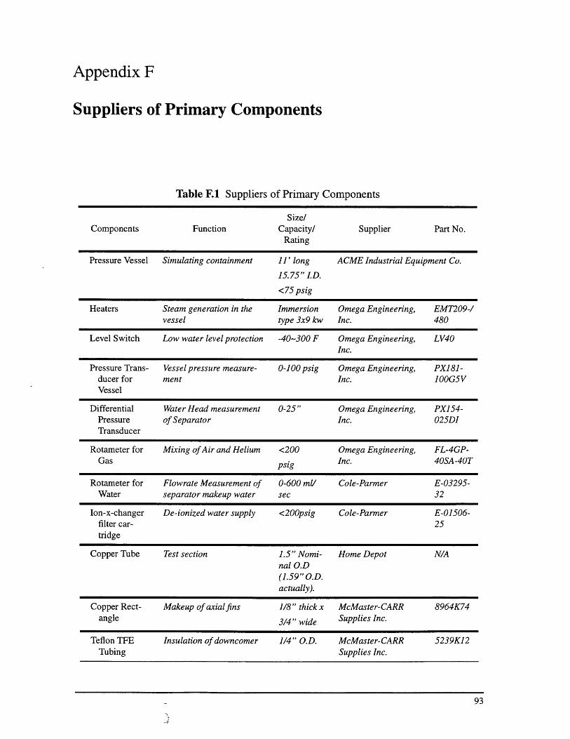
Appendix F

Suppliers of Primary Components

Table F.1 Suppliers of Primary Components

Size!Components Function Capacity/ Supplier Part No.

Rating

Pressure Vessel Simulating containment 11' long ACME Industrial Equipment Co.

15.75" I.D.

<75 psig

Heaters Steam generation in the Immersion Omega Engineering, EMT209-/vessel type 3x9 kw Inc. 480

Level Switch Low water level protection -40-300 F Omega Engineering, LV40Inc.

Pressure Trans- Vessel pressure measure- 0-100 psig Omega Engineering, PX181-ducer for ment Inc. J00G5VVessel

Differential Water Head measurement 0-25" Omega Engineering, PX154-Pressure of Separator Inc. 025DITransducer

Rotameter for Mixing of Air and Helium <200 Omega Engineering, FL-4GP-Gas psig Inc. 40SA-40T

Rotameter for Flowrate Measurement of 0-600 ml/ Cole-Parmer E-03295-Water separator makeup water sec 32

Ion-x-changer De-ionized water supply <200psig Cole-Parmer E-01506-filter car- 25tridge

Copper Tube Test section 1.5" Nomi- Home Depot N/Anal O.D(1.59" O.D.actually).

Copper Rect- Makeup of axial fins 1/8" thick x McMaster-CARR 8964K74angle 3/4" wide Supplies Inc.

Teflon TFE Insulation of downcomer 1/4" O.D. McMaster-CARR 5239K12Tubing Supplies Inc.

93

Table F.1 Suppliers of Primary Components

Size/Components Function Capacity/ Supplier Part No.

Rating

PVC sewer Shroud for smooth tube 4" I.D. & McMaster-CARR 2426K12pipe 10' long Supplies Inc.

Thermocouples Temperature Measurement 1/16" SS Omega Engineering, GTQSS-Sheathed Inc. 116G

Temperature Power supply control for PID control Borrowed from MIT Fusion CenterController the vessel (Contact Peter Stahle)

J-type Exten- Thermocouple wire exten- J-type Omega Engineering, FF-J-24sion wire sion Inc.

Multiconduc- Compressionfitting for 16 channel Omega Engineering, MFT-116-tor thermocouples through the for 1/16" Inc. 16Feedthrough vessel lid SS

SheathedTCs

Silicon Rubber Sealing of separator 1/2 "thick McMaster-CARR 8632K46Gasket Supplies Inc.

Fiberglass Vessel insulation 1" thick McMaster-CARR 5556k55Supplies Inc.

Elastomeric Insulation of the Separator 1.5" thick McMaster-CARR 9349K5PVC Foam Supplies Inc.

Reinforced Steam venting 2" I.D. McMaster-CARR 5301K16EPDM Rub- Supplies Inc.ber SteamHose

Silicon Rubber Provide flexible connec- 4" I.D. McMaster-CARR 5296K48Hose tion between the vessel <500 F Supplies Inc.

and the separator

Safety Valve Over-Pressure protection 75 psig McMaster-CARR 4712k52of the Vessel Supplies Inc.

Connection Makeup of recirculation Supplied by McMaster-CARR Supplies Inc.Piping and loopFittings

DATACQ.BAS Source code of Data Developed by Haiyang Liu. Stored in the floppy diskAcquisition Program in the possession of the NED Computer Facility

Administrator

94

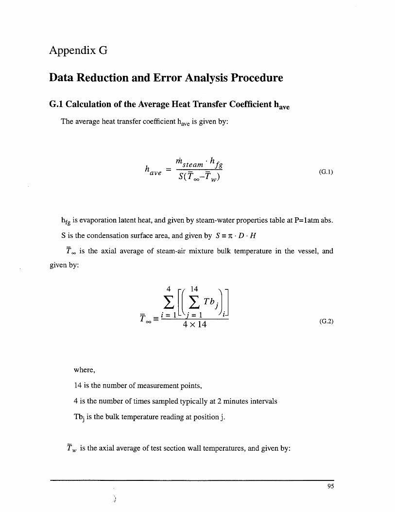
Appendix G

Data Reduction and Error Analysis Procedure

G.1 Calculation of the Average Heat Transfer Coefficient have

The average heat transfer coefficient have is given by:

h av steam - h.ave -S(T.-TW)

hfg is evaporation latent heat, and given by steam-water properties table at P=latm abs.

S is the condensation surface area, and given by S= 7 -D -H

U, is the axial average of steam-air mixture bulk temperature in the vessel, and

given by:

4 r14

I I Tb

4 x14 (G.2)

where,

14 is the number of measurement points,

4 is the number of times sampled typically at 2 minutes intervals

Tbj is the bulk temperature reading at position j.

TW is the axial average of test section wall temperatures, and given by:

95

4 6

W4x6 (G.3)

where

6 is the number of measurement points,

4 is the number of times sampled

Twj is the wall temperature reading at position j.

steam is the mass flow rate of steam evaporated from the coolant in the separator

and recirculation loop, and is given by

msteam = a - 1sep (G.4)

where,

Psep is the rate of the pressure change at the bottom of the separator due to the

internal water inventory change

a is a constant, mathematically given by a = g/Scro and experimentally calibrated

by the d.p. cell and the rotameter for the measurement of the separator makeup water flow-

rate. The calibration process is as follows:

1. Inject room temperature water into the separator through the rotameter;

2. Use the d.p. cell and a timer to measure Pcali;

3. Use the rotameter to measure the water mass flowrate ticali

4. Use a least-square-fit to get a from the relation:

mecalia = .a (G.5)

Pcali

96

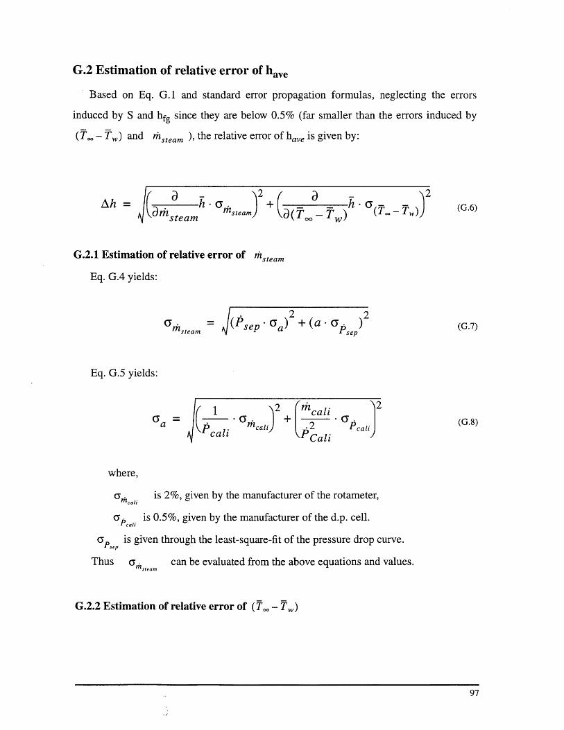
G.2 Estimation of relative error of have

Based on Eq. G.1 and standard error propagation formulas, neglecting the errors

induced by S and hfg since they are below 0.5% (far smaller than the errors induced by

(T. -,) and tisteam ), the relative error of have is given by:

Ah= ah- + _ _ h-(T- - (G.6)FF s team hsteam) a(T; - TO) (.-

G.2.1 Estimation of relative error of thsteam

Eq. G.4 yields:

G thsteam = A(Psep Ga)2 + (a - a ep 2 (G.7)

Eq. G.5 yields:

12 rhcali 2

P mcali + cali2 PcaliJ

PCali

where,

a t is 2%, given by the manufacturer of the rotameter,

Ga is 0.5%, given by the manufacturer of the d.p. cell.

CY ' is given through the least-square-fit of the pressure drop curve.

Thus a can be evaluated from the above equations and values.

G.2.2 Estimation of relative error of (Tc, - Tw)

97

The relative error of (T. - T,) can be directly derived from the error propagation

formula, i.e.:

2 2G(T- ) T +Y (G.9)

where,

4- 2

(Tbk Tb)

2 _ k=1TO 4 (G.10)

4-2

(Twk-Tw)

2 _ k=lG 4 (G.11)

Equ. G. 10 and G. 11 are obtained directly from the standard deviation formula.

G.2.3 Summary

The average heat transfer coefficient have is calculated from G.1 to G.5.

The relative error of (T,. - Tw) is calculated from Eq. G.9, G.10 and G.1 1.

Section G.2.1 and G.2.2 present the complete solution of the relative error of have-

The typical values for the relative error of have are 17% for have < 600 w/(mA2*s) and

8% for have > 600 w/(mA2*s). The measurement errors vary with the heat transfer coeffi-

cient because for the lower have cases, there exists a relatively unstable natural circulation,

thus less uniform temperature distribution, which leads to a higher relative error of

(T"O - %,). In high have cases the measurement error of the steam flowrate plays the dom-

inant role in generating the relative error of have. In low have cases the wall temperature

variation accounts for most of the relative error of have.

98

Appendix H

Standard Operating Procedure (SOP)

Part 1. Standard facility Pre-Power-Operating operations

1.0 General inspection

1.0.1 Confirm that all power switches(480 V, 120 V heating, 120 V control power) are

in "OFF" positions.

1.1 Operations on the first floor

1.1.1 Inspect vessel bottom on the first floor; Confirm that penetrations are leak-free

and all cables are correctly connected and in good condition.

1.1.2 Check to insure vessel bottom drain valve is in closed position.

1.1.3 Confirm that plastic tarpaulin covers the exclusion area -- the hatch under the

vessel.

1.1.4 Close the cage and place the sign "Experiment is on, please keep off'.

1.1.5 Switch the "480 V power supply switch 2" near the cage to the "ON" position.

1.2 Operations on the second floor

1.2.1 Inspect vessel top lid and confirm that all fittings are in place and tight and sepa-

rator steam venting line is connected.

1.2.2 Open "normal relief valve".

1.2.3 Switch "3-channel valve" to vessel water supply position.

1.2.4 Open "vessel water injection valve".

99

1.2.5 Inject 114 liters of DI water from the makeup water supply subsystem by timing

flowmeter rate (max= 600 CC/min for 190 mins). This will fill vessel to depth of around

2.5 ft and cover heaters to a depth of -10 inches.

1.2.6 Shut off "normal relief valve".

1.2.7 Shut off "vessel water injection valve".

1.2.8 Switch "3-channel valve" to separator water supply position.

1.2.9 Inject DI water to fill separator to a water level of around 3 in from the bottom.

1.2.10 Confirm steam venting line is connected.

Part 2. Standard Power on/off operations

2.1 Power on operations

2.1.1 Confirm that there is enough water in vessel (refer to 1.2.5)

2.1.2 Switch "control power" on.

2.1.3 Check/set temp1 alarm temperature to desired value (default value =300 F).

2.1.4 Check/set temp2 alarm temperature to desired value (default value =300 F).

2.1.5 Check/set temp2 working temperature according to specific run, (default

value=212 F).

2.1.6 Cancel alarm lights (refer to Table 1) by pushing corresponding buttons.

2.1.7 Confirm there are no alarm lights on or take corrective actions as indicated in

Table 1.

2.1.8 Switch the "480 V Power Supply Switch 0" on the wall of NW13-253 labroom

to the "ON" position.

2.1.9 Check/set temp2 power control to "manual" or"Auto" mode and check corre-

sponding parameters--power percentage for "manual" mode; operation loop set for "Auto"

mode. (refer to Temperature Controller Manual)

2.1.10 Switch the "480 V Power Supply Switch 1" on the control panel to the "ON"

position.

100

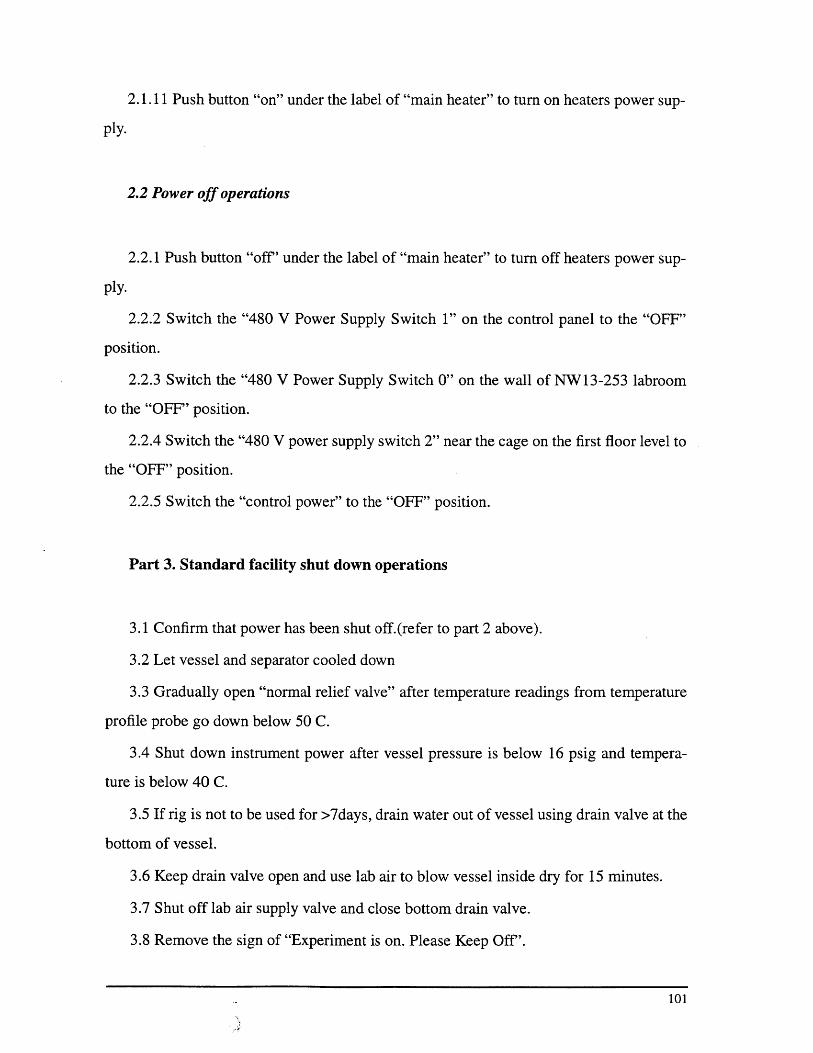
2.1.11 Push button "on" under the label of "main heater" to turn on heaters power sup-

ply.

2.2 Power off operations

2.2.1 Push button "off' under the label of "main heater" to turn off heaters power sup-

ply.

2.2.2 Switch the "480 V Power Supply Switch 1" on the control panel to the "OFF"

position.

2.2.3 Switch the "480 V Power Supply Switch 0" on the wall of NW13-253 labroom

to the "OFF" position.

2.2.4 Switch the "480 V power supply switch 2" near the cage on the first floor level to

the "OFF" position.

2.2.5 Switch the "control power" to the "OFF" position.

Part 3. Standard facility shut down operations

3.1 Confirm that power has been shut off.(refer to part 2 above).

3.2 Let vessel and separator cooled down

3.3 Gradually open "normal relief valve" after temperature readings from temperature

profile probe go down below 50 C.

3.4 Shut down instrument power after vessel pressure is below 16 psig and tempera-

ture is below 40 C.

3.5 If rig is not to be used for >7days, drain water out of vessel using drain valve at the

bottom of vessel.

3.6 Keep drain valve open and use lab air to blow vessel inside dry for 15 minutes.

3.7 Shut off lab air supply valve and close bottom drain valve.

3.8 Remove the sign of "Experiment is on. Please Keep Off'.

101

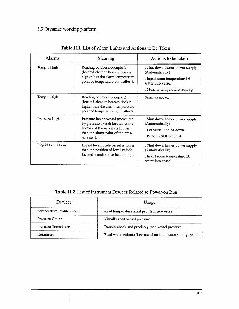
3.9 Organize working platform.

Table H.1 List of Alarm Lights and Actions to Be Taken

Alarms Meaning Actions to be taken

Temp 1 High Reading of Thermocouple 1 . Shut down heater power supply(located close to heaters tips) is (Automatically)higher than the alarm temperature . Inject room temperature DIpoint of temperature controller 1. water into vessel

. Monitor temperature reading

Temp 2 High Reading of Thermocouple 2 Same as above.(located close to heaters tips) ishigher than the alarm temperaturepoint of temperature controller 2.

Pressure High Pressure inside vessel (measured . Shut down heater power supplyby pressure switch located at the (Automatically)bottom of the vessel) is higher . Let vessel cooled downthan the alarm point of the pres- Perform SOP step 3.4sure switch

Liquid Level Low Liquid level inside vessel is lower . Shut down heater power supplythan the position of level switch (Automatically)located 1 inch above heaters tips. . Inject room temperature DI

water into vessel

Table H.2 List of Instrument Devices Related to Power-on Run

Devices Usage

Temperature Profile Probe Read temperature axial profile inside vessel

Pressure Gauge Visually read vessel pressure

Pressure Transducer Double-check and precisely read vessel pressure

Rotameter Read water volume flowrate of makeup water supply system

102

Appendix I

Code for Data Reduction

I.1 Source CodeFile Name: DRC.C

Suggested Compiler: GNU C++ Compiler on Sun Sparc Workstations

#include <iostream.h>

#include <fstream.h>

#include <string.h>

#include <stdlib.h>

#include <stdio.h>

#include <math.h>

//------------------ classes definitions ----------------------

class seriesno {public:

char runno[30];

int timeno;

seriesnoo I

I;

class vessel {public:

double g.Ltotpres,t_totpres;

double temp-prof[16],vliqlevel;

double pos.tf[ 16];//postions of measuring points of TF , assigned permenantly

vessel() { gtotpres=O.O;t_totpres=0.0;

for(int i=O;i< 1 6;i++) { tempprof[i]=O.O;}

vliqjevel=0.0;

}};

103

class separator {

public:

double smakeup-jemp,smakeup-pres;

double recirout-temp,recir intemp;

double ssteamtemp,ssteampres;

double bulktemp, bot_pres;

double sliq-levelriserheight;

separatoro{smakeup-jemp=0.0; smakeup-pres=0.0;

recirout-temp=O.O;recirjintemp=0.0;

ssteamjtemp=O.O;ssteam pres=0.0;

bulktemp=0.0; botpres=0.0;

sliq_level=0.0; riser-height=0.0;

}

class testedtube {

public:

double coolantoutjtemp,coolant injtemp;

double surftemp[6];

double posjtc[6]; //postions of 6 TCs , assigned permenantly

testedtubeo { coolantouttemp=O.O;coolantintemp=0.0;

for(int i=O;i<6;i++) surf temp[i]=O.O;

}};

class makeupwater {

public:

double makeupjemp,makeuppres,flow reading,rel error;

104

double evec;

makeupwaterO {

makeup-temp=O.O;makeup-pres=O.O;flow reading=0.0;

ev=O.O;ec=0.0;

}

class steamventing{

public:

double vsteamtemp,vsteampres;

double heaterjv,heater_c, heaterpower;

double temp-before heating, temp-after heating;

steamventingo {

vsteamtemp=O.O;vsteam~pres=0.0;

heater_vheaterc=0.0; heater-power=O.O;

tempjbefore heating=0.0; temp-after-heating=0.0;

}};

class pre-proc {

public:

int data-no;

double sdata[40];

double avevalsdVal;

void ave std(){

int i;

double ave=O.O,sd=0.0;

/compute average value

for(i=O;i<data-no;i++) ave=ave+sdata[i];

105

ave_val=ave/datano;

// compute standard deviation

for(i=0;i<datano;i++) sd=sd+(sdata[i]-ave-val)*(sdata[i]-ave-val);

sdval=sd/(data-no- 1);

}

preproco I

};

class Record:

public seriesno, public vessel,

public separator, public testedtube, public makeupwater,

public steamventing, public pre-proc

{public:

double TbulkbarTwallbar, dTbar;

RecordO {

Tbulkbar=0.0;

Twallbar=0.0;

dTbar=0.0;

} /constructor

read(int n){

int j;char trival[12];

//read run No.

cin>>runno>>timeno;

/read vessel data

106

cin>>g-jotpres>>t-totpres;

for(j=O;j<1 6;j=j+1) cin>>temp-profj];

cin>>vliq_level;

/read separator data

cin>>smakeupjtemp>>smakeup-pres;

cin>>recirouttemp>>recirinjtemp;

cin>>ssteamjtemp>>ssteampres;

cin>>bulkjtemp>>bot-pres;

cin>>sliq level>>riserjheight;

/read testedtube data

cin>>coolantintemp>>coolant outtemp;

for(j=O;j<6;j=j+1) cin>>surf temp[j];

/read makeup-water data

cin>>makeup-temp>>makeup-pres;

if (n==O) cin>>flowjreading>>relerror;

//only read flowreading from the first record

else cin>>trival;

cin>>ev>>ec;

/read steamventing data

cin>>vsteamjtemp>>vsteam~pres;

cin>>heater_v>>heater_c>>heaterpower;

cin>>tempbefore-heating>>temp-after heating;

} // end of readO

/----------------

write (){

107

int j;

//write run No.

cout<<runno<<" "<<timeno<<endl;

//write vessel data

cout<<g-jotpres<<" "<<t_totpres<<endl;

for(j=O;j<1 6;j=j+1) cout<<temp-profj]<<endl;

cout<<vliqjlevel<<endl;

//write separator data

cout<<smakeup-jemp<<" "<<smakeup-pres<<endl;

cout<<recirouttemp<<" "<<recirinjtemp<<endl;

cout<<ssteamtemp<<" "<<ssteam-pres<<endl;

cout<<bulktemp<<" "<<botpres<<endl;

cout<<sliqjlevel<<" "<<riser-height<<endl;

//write testedtube data

cout<<coolantin-temp<<" "<<coolantout-temp<<endl;

for(j=O;j<6;j=j+1) cout<<surftempU]<<endl;

//write makeup-water data

cout<<makeup-jemp<<" "<<makeup-pres<<" "<<flowreading<<endl;

cout<<ev<<" "<<ec<<endl;

//write steamventing data

cout<<vsteamtemp<<" "<<vsteam-pres<<endl;

cout<<heater_v<<" "<<heater_c<<" "<<heater-power<<endl;

cout<<temp-before heating<<" "<<temp-after heating<<endl;

I // end of writeo

108

//----------get dT for this record

get-dT(){

int k;

for(k=0;k< 14;k++)

if (k!=10) Tbulkbar=Tbulkbar+temp-prof[k]; /skip the failed 11 th TC

I

Tbulkbar=Tbulkbar/13.0;

for(k=0;k<6;k++) Twall-bar=Twallbar+surfitemp[k];

Twallbar=Twallbar/6.0;

dTbar=Tbulkbar-Twallbar;

}I/ end of ---- getdT

}; /end of class Record

class Property

{

public:

double p[50],dh[50];

double step; //t step 1 C

int start_t;//start from 100 c

PropertyO)

startt=100;

step= 1.0;

p[O]=9.2/100000.;

p[1]=0.5324;

p[2]=1.0806;

p[3]=1.645;

109

p[4 ]=2.2259;

p[5]=2.8239;

p[6 ]=3.4391;

p[7 ]= 4 .0721;

p[8]= 4 .7232;

p[ 9]=5.3927;

p[10]= 6 .0812;

p[ 11]=6.7889;

p[1 2 ]=7.5163;

p[13]=8.2639;

p[14 ]= 9 .0319;

p[15]=9.8210;

p[16]=10.631;

p[17]=1 1.464;

p[18]=12.318;

p[1 9 ]=13.195;

p[20]=14.096;

p[21]=15.020;

p[22]=15.968;

p[2 3 ]=16.940;

p[24]=17.938;

p[ 2 5 ]=18.961;

p[26]=20.010;

p[2 7 ]=21.085;

p[28]=22.188;

p[29]=23.318;

p[3 0]= 2 4.476;

p[31]=25.662;

p[ 3 2 ]= 2 6 .877;

p[33]=28.122;

p[34]=29.397;

p[ 3 5 ]=30.702;

110

p[36]=32.039;

p[37]=33.407;

p[38]=34.807;

p[39]=36.241;

p[40]=37.707;

HI--------

dh[0]=2256.;

dh[1]=2253.4;

dh[2]=2250.7;

dh[3]=2248.0;

dh[4]=2245.3;

dh[5]=2242.7;

dh[6]=2240.;

dh[7]=2237.3;

dh[8]=2234.5;

dh[9]=2231.8;

dh[10]=2229.1;

dh[1 1]=2226.4;

dh[12]=2223.6;

dh[13]=2220.9;

dh[14]=2218.1;

dh[15]=2215.3;

dh[16]=2212.6;

dh[17]=2209.8;

dh[18]=2207.0;

dh[19]=2204.2;

dh[20]=2201.4;

dh[21]=2198.6;

dh[22]=2195.7;

dh[23]=2192.9;

dh[24]=2190.;

dh[25]=2187.2;

111

dh[26]=2184.3;

dh[27]=2181.4;

dh[28]=2178.5;

dh[29]=2175.6;

dh[30]=2172.7;

dh[3 1]=2169.8;

dh[32]=2166.9;

dh[33]=2164.;

dh[34]=2161.;

dh[35]=2158.1;

dh[36]=2155.1;

dh [37]=2152. 1;

dh[38]=2149.1;

dh[39]=2146.1;

dh[40]=2143.1;

double get sat pres(double t)

{int low=((int) t)-startt, high=low+1;

return p [low]+((t-low-start-t)/step)*(p[high]-p[low]); /psig

double get-evapjheat(double t)

{int low=((int) t)-100,high=low+1;

return (dh[low]+((t-low-start-t)/step)*(dh[high]-dh[low]))*1000.0; //j/kg

}

112

class AirFra

{

public:

double airjfra[14]; //15,16 are submerged under water

double temp[16];

const double mr=29./18.;//ratio of Melocular mass of steam to air

double Pt;

Property pro;

AirFra(int n,double t[],double pt){

for(int i=O;i<n;i++) temp[i]=t[i];

Pt=pt+14.7; //psia

I

compute(){

double Ps;

for(int i=O;i<14;i++)

if (i!=11){

Ps=pro.get sat-pres(temp[i])+14.7; //psia

// cout<<Ps<<endl;

air fra[i]=(mr*((Pt-Ps)/Ps))/(1+(mr*((Pt-Ps)/Ps))); /P29 Dehbi

}}

}

};

113

/----------------- end of classes definition -----------------

/---------------- start of main code ---------------------------

main(int argc, char *argv[])

{int i=Oj=O,step=6,RecCounter=O;

char ff[12],tmp[100];

Record r[40],ave,std;

pre-proc t;

/--------------------

// Read data from file +

/-----------------------

cin.clearo;

while(1)

{cin>>tmp;

if(cin.eofO) break;

r[Rec Counter].read(RecCounter);

//r[i].writeO;

RecCounter++; /counter of records

I

RecCounter--; //modify the effect of CZ at the end of each input datafile

/end of reading----

/------------------

I/ Statistical Analysis

/-----------------

114

// compute averages and standard differences of all parameters based on

// all serial data sources files for the same RUN condition

ave.runno=r[O].runno;

std.runno=r[O].runno;

t.datano=RecCounter;

//-- g-totpres

for (i=O;i<RecCounter;i++)

{t.sdata[i]=r[i].g-jotpres;

}t.ave-stdo;

ave.g_totpres=t.aveival;

std.gjtotpres=t. sdval;

cout<<t.datano <<endl;

//-- tjtotpres


{t.sdata[i]=r[i].t.totpres;

}t.ave-stdo;

ave.tLtotpres=t.aveval;

std.tLtotpres=t.sd-val;

//-- temp_prof[16]

115

for(j=O;j<16;j++){


{t.sdata[i]=r[i].temp-profU];

}t.avestdo;

ave.temp-profj]=t.ave-val;

std.tempprofU]=t.sd-val;

}//-- vliqjevel


{t.sdata[i]=r[i].vliq_level;

}t.avestdo;

ave.vliqjlevel=t.ave val;

std.vliqjlevel=t.sd-val;

//-- smakeupjtemp


{t.sdata[i]=r[i].smakeuptemp;

t.avestdo;

ave.smakeup-jemp=t.aveval;

std.smakeup-jemp=t.sdval;

//-- smakeup-pres


116

{

t.sdata[i]=r[i].smakeup-pres;

I

t.avestdo;

ave.smakeup-pres=t.ave_val

std.smakeup-pres=t.sdval;

//-- recirouttemp


t.sdata[i]=r[i].recir-outtemp;

I

t.ave-stdo;

ave.recirouttemp=t.aveval;

std.recirouttemp=t.sdval;

//-- recirintemp


t.sdata[i]=r[i].recir-intemp;

t.avestdo;

ave.recirintemp=t.aveval;

std.recirintemp=t.sd-val;

//-- ssteamtemp


{

{

}

117

{t.sdata[i]=r[i].ssteamtemp;

}t.avestdo;

ave.ssteamtemp=t.ave-val;

std.ssteamtemp=t.sd val;

//-- ssteampres


{t.sdata[i]=r[i].ssteamnpres;

}t.avestdo;

ave.ssteampres=t.aveval;

std.ssteam-pres=t.sd val;

//-- bulk_temp


{t.sdata[i]=r[i].bulkjtemp;

}t.ave-stdo;

ave.bulkjtemp=t.aveval;

std.bulkjtemp=t.sdval;

//-- bot-pres


{

t.sdata[i]=r[i] .bot~pres;

}

118

t.ave-stdO;

ave.bot-pres=t.aveval;

std.bot-pres=t.sdjval;

//-- sliqilevel


{t.sdata[i]=r[i].sliqjevel;

}t.ave-stdo;

ave.sliqjevel=t. aveval;

std.sliqjevel=t.sdval;

//-- riserheight


{t.sdata[i]=r[i].riser.height;

}t.ave-stdo;

ave.riser-height=t.ave val;

std.riser-height=t.sdval;

//-- coolantintemp


{t.sdata[i]=r[i].coolantinjtemp;

}t.ave-stdo;

ave.coolantinjtemp=t.aveval;

std.coolantinjtemp=t.sd_val;

119

//-- coolantouttemp


{t.sdata[i]=r[i].coolantoutjtemp;

}t.avestdo;

ave.coolantout-temp=t.aveval;

std.coolantoutjtemp=t.sdval;

//-- surftempj]

for(j=O;j<6;j++){


{t.sdata[i]=r[i].surf temp[j];

}t.avestdo;

ave.surf temp[j]=t.aveval;

std.surf tempj]=t.sdval;

}

//-- makeup-temp


{t.sdata[i]=r[i].makeuptemp;

}t.avestdo;

ave.makeup-jemp=t.aveval;

std.makeup-temp=t.sd-val;

//-- makeup-pres

120


{t.sdata[i]=r[i].makeup-pres;

}t.avestdo;

ave.makeup-pres=t.ave val;

std.makeup-pres=t.sd val;

//-- flowreading

/* for (i=O;i<Rec_Counter;i++)

{t.sdata[i]=r[i].flowreading;

}t.avestdo;

ave.flowreading=t.ave-val;

std.flowreading=t.sdyval;*/

ave.flowreading=r[O].flowreading;

std.flowreading=

(r[O].rel_error*r[O].flow-reading)*(r[O].rel_error*r[O].flowreading);

for (i=O;i<Rec_Counter;i++)

{t.sdata[i]=r[i].ev;

}t.ave-stdo;

ave.ev=t.aveval;

std.ev=t.sd_val;

//-- ec


{

121

t.sdata[i]=r[i].ec;

}t.ave-stdo;

ave.ec=t.aveval;

std.ec=t.sd_val;

//-- vsteamjtemp


{t.sdata[i]=r[i].vsteamtemp;

}t.avestdo;

ave.vsteamtemp=t.ave val;

std.vsteam_temp=t.sdval;

//--vsteampres


{t.sdata[i]=r[i].vsteampres;

}t.ave-stdo;

ave.vsteam-pres=t.aveval;

std.vsteam-pres=t.sd val;

//-- heater-v


{t.sdata[i]=r[i].heater_v;

}t.avestdo;

ave.heaterv=t. aveVal;

std.heaterv=t.sd-val;

122

/-- heater_c

for (i=0;i<RecCounter;i++)

t.sdata[i]=r[i].heater-c;

t.ave-stdo;

ave.heaterc=t.ave-val;

std.heaterc=t.sdval;

//-- heater-power


t.sdata[i]=r[i].heaterpower;

t.ave-stdo;

ave.heater-power=t.ave val;

std.heater-power=t.sdval;

//-- temp-before heating


t.sdata[i]=r[i].tempbefore heating;

t.avestdo;

ave.tempbefore heating=t.aveval;

std.tempbefore-heating=t.sd val;

/-- temp-after heating

123

{

}

{

}

{

}

for (i=0;i<RecCounter;i++)

{t.sdata[i]=r[i].tempafterheating;

}t.ave-stdo;

ave.temp-after heating=t.ave Val;

std.temp-after heating=t.sdVal;

/------------end of Statistical Analysis------------

/*

cout<<RecCounter<<endl;

ave.writeo;

std.writeO;

*/

/----------------------------

// Air Mass Fraction Computation +

/----------------------------

AirFra af(16,ave.temp-prof,ave.tjtotpres); //initialize af

af.computeo; //from now on the airjfra[0-13] available

double ave_af=0.0;

for(i=O;i< 1 4;i++) {

aveaf=aveaf+af.air-fra[i];}

aveaf=aveaf/14; /average air fraction;

// ----- end of Air Mass Fraction Computation ---

124

//--------------------------------------------------------

// Average Twall, Tbulk for steam-air and dTComputation

/----------------------------------------------------

int kk;

preproc tdT;

+

for(kk=O;kk<RecCounter;kk++)

r[kk].get_dTO;

t_dT.datano=RecCounter;

for(kk=O;kk<tdT.data no;kk++) tdT.sdata[kk]=r[kk].dTbar;

t_dT.avestdO;

double finaldTbar=t_dT.aveval;

double finaldelta_dTbar=sqrt(t_dT.sd-val); /final average dT and standrad

deviation


for(kk=O;kk<tdT.datano;kk++) tdT.sdata[kk]=r[kk].Tbulkbar;

t_dT.avestd(;

double final_Tbulk_bar=t_dT.ave_val;/ final average Tbulk


for(kk=O;kk<tdT.datano;kk++) t dT.sdata[kk]=r[kk].Twall-bar;

t_dT.avestdO;

double finalTwallbar=t_dT.aveval; / final average Twall

II--- end of Average Twall, Thulk for steam-air Computation

125

// --------------------------------------------------

/ average h Computation +

/---------------------------------------

Property pro;

double aveden=957.0; /ave water density inside test tube (Kg/mA3)

double height=78*2.54/100.;//height(m) 78"+3"

double dP=(aveden*9.8*height)/10 1300.0*14.7; //dP (Pa)

double Pout=ave.bot-pres,Pin=Pout+dP; //psi

double Tout=ave.reciroutjtemp,Tin=ave.recir intemp; I/c

double dh=pro.get evap_heat(Tout); //evaparation heat (J/kg)

double D=1.625*2.54/100.; //(m) diameter of test tube

double area=3.14*D*height; /area of test section mA2

double volflowrate=ave.flowreading*835.4/1000000.; //mA3/s

// flowreading is reading unit/sec, 835.4 ml/reading unit

double den_makeup=994.5; //DI makeup water density (Kg/mA3)

double massflowrate=volflowrate*denmakeup; //kg/s

double h; /ave heat trasnfer coeff

h=massflowrate*dh/(finaldTbar*area); // w/(C*mA2)

// ---- end of average h Computation --

126

'4

//---------------------------------------

// Error Analysis

I-----------------------------------

double delta_a=0.04; //from manufacturer

double deltaMassFlowrate=

sqrt(r[O].rel-error*r[O].relerror+deltaa*delta-a)*massflowrate; //directely

given from the first record

double dhm=dh/(finaldTbar*area);

// double dhdh=massflowrate/(avedT*area);

double dhdT=massflowrate*dh/(area*finaldTbar*finaldT-bar);

// delta_h_bar

double delta_h-bar=sqrt(

(dh-m*deltaMassFowrate)*(dh-m*deltaMassFlowrate)+

(dh-dT*final-delta-dT-bar)*(dh-dT*final-delta dT-bar)

double hrelativeerror=delta_h_bar/h;

//------ end of Error Analysis --

//---------------------------------

// Results output +

/--------------------------

cout<<" Run No."<<" "<<"Air Mass Fraction"<<" "<<

"dT(Celcius)"<<" "<<"Pt (Psig)"<<" "<<"h (w/(mA2*C)"<<endl;

cout<<ave.runno<<" "<<aveaf<<" "<<finaldTbar<<" "<<

ave.ttotpres<<" "<<h<<endl<<endl<<endl;

127

cout<<"Tw="<<final_Twallbar<<" "<<"Tbulk="<<finalTbulkbar<<endl;

cout<<"The total heat transfer rate is (kW): "<<massflowrate*dh/lOOO.<<endl;

cout<<"The average h is: "<<h<<"+/-"<<delta_h_bar<<endl;

cout<<"The relative error of h is: "<<h_relativeerror<<endl;

// cout<<massflowrate<<" " <<dh<<endl;

//end of program

}

1.2 Sample Input and OutputSample Input

*** ** *** ***** *************

RUN5_1.DAT

1

52.149 52.149

109.1338 109.5732 111.168 111.918 112.4961 113.0625 112.8916 113.2627

113.9053 114.4932 9.999999E+37 114.5674 114.4531 113.166 147.4912

147.4131

21.68

80 16.10

101.0479 99.81934

99.40918 0.0

99.81934 0.00

21.8

0.00

100.0674 101.0479

105.5391 105.5215 106.0117 105.7227 105.9844 105.8916

80 16.10

0.000422 0.038

128

120 10.0

99.40918 0.0

120 5.0 600.0

000 000

RUN5_1.DAT

2

52.26776 52.26776

109.9629 110.6562 110.9678 111.2969 111.3926 111.8115

113.1719 113.4658 114.0684 9.999999E+37

147.6504 147.292

21.68

80 16.10

101.3252 99.75781

114.9971 114.8281 113.9785

99.39453 0.0

99.75781 0.00

21.8

0.00

99.91699 101.3252

102.666 102.9307 102.2314 102.2988 102.3066 102.498

80 16.10

120 10.0

99.39453 0.0

120 5.0 600.0

000 000

129

112.1162

RUN5_1.DAT

3

52.349 52.349

110.5596 110.6152 111.6641 111.9033 111.6338 111.9062 111.6758113.4707 113.1016 113.3965 697.3467 115.2646 115.4658 114.5029 147.7188147.3252

21.68

80 16.10

100.917 99.90722

99.40625 0.0

99.90722 0.00

21.8

0.00

100.2754 100.917

105.3496 105.5029 105.3604 105.0947 105.7676 105.0234

80 16.10

120 10.0

99.40625 0.0

120 5.0 600.0

000 000

* ** * ********** ***** ***** **** *****

RUN5_1.DAT

4

52.31425 52.31425

130

110.2021 110.4229 110.4482 110.7402

113.3398 113.9492 114.8682 9.999999E+37

147.5781 147.3662

21.68

80 16.10

101.0029 99.83105

110.8662 112.1543 112.3086

115.6055 115.4473 115.5732

99.41504 0.0

99.83105 0.00

21.8

0.00

100.1211 101.0029

104.6611 104.626 105.374 105.708 105.7451 105.4619

80 16.10

120 10.0

99.41504 0.0

120 5.0 600.0

000 000

Sample Output

Air Mass Fraction dT(Celcius) Pt (Psig) h (w/(mA2*C)

RUN5_1.DAT 0.711682 7.80064 52.323 394.407

Tw=104.935 Tbulk=112.736

The total heat transfer rate is (kW): 0.789987

The average h is: 394.407+/-67.7449

The relative error of h is: 0. 171764

131

Run No.

An Experimental Investigation of A Passive Cooling Unit ...

Documents

Transcript of An Experimental Investigation of A Passive Cooling Unit ...