AN EXPERIMENTAL COMPARISON OF NONSWIRLING AND SWIRLING

FLOW IN A CIRCULAR-TO-RECTANGULAR TRANSITION DUCT

Abstract

Circular-to-rectangular transition ducts are used as

exhaust system components of aircraft with rectangularexhaust nozzles. Often, the incoming flow of these tran-

sition ducts includes a swirling velocity component re-

maining from the gas turbine engine. Previous transitionduct studies have either not included inlet swirl or when

inlet swirl was considered, only overall performance pa-

rameters were evaluated. This paper explores circular-to-

rectangular transition duct flows with and without inletswirl in order to understand the effect of inlet swirl on

the transition duct flow field and to provide detailed duct

flow data for comparison with numerical code predictions.

A method was devised to create a swirling, solid

body rotational flow with minimal associated distur-bances. Coefficients based on velocities and total and

static pressures measured in cross stream planes at four

axial locations within the transition duct, along with sur-

face static pressure measurements and surface oil film

visualization, are presented for both nonswirling and

swirling incoming flow. In both cases the inlet centerline

Mach number was 0.35. The Reynolds number based on

the inlet centerline velocity and duct inlet diameter was1,547,000 for nonswirling flow and 1,366,000 for swirling

flow. The maximum swirl angle was 15.6 ° . Two pair of

counter-rotating side wall vortices appeared in the ductflow without inlet swirl. These vortices were absent in

the swirling incoming flow case.

Introduction

Nonaxisymmetric exhaust nozzles are employed on

high performance aircraft to improve performance. Rect-angular exhaust nozzles require a circular-to-rectangular

transition duct to connect the engine and nozzle. To max-

imize nozzle performance the transition duct should min-

imize transverse velocity components at the duct exit and

the total pressure loss in the duct.

In typical exhaust component applications the in-

coming flow to the circular-to-rectangular transition duct

*Research Engineer, Inlet, Duct, and Nozzle Flow

Physics Branch.

tResearch Engineer, Inlet, Duct, and Nozzle Flow

Physics Branch, Member AIAA.

*Professor and Chair, Mechanical Engineering De-

partment, Member AIAA

B.A. Reichert* and W.R. Hingst t

National Aeronautics and Space AdministrationLewis Research Center

Cleveland, Ohio 44135and

T.H. Okiishi*

Iowa State UniversityAmes, Iowa 50010

is turbulent, subsonic, and not fully developed. Often,

the incoming flow includes a significant rotational veloc-

ity component. The term swirl refers to this rotational

velocity component, which remains from the engine tur-

bine. Representative studies of turbine exit flow angles 1-3

have shown that swirl often exists at turbine design op-

erating conditions, and may be as great as 30 ° or more

at off-design operating conditions. Inlet swirl can signif-

icantly alter the flow field throughout the transition duct.

Previous researchers have experimentally explored

the aerodynamics of circular-to-rectangular transitionducts. Patrick and McCormick 4' 5 recorded values of total

pressure, mean velocity, and three normal Reynolds stress

components at the inlet and exit planes of two differ-

ent circular-to-rectangular transition ducts. Miau et al. 6' 7measured mean velocities and turbulence intensities at

the inlet and exit of three circular-to-rectangular transi-

tion ducts. In a benchmark study, Davis and Gessner 8

measured static pressures, mean velocities, and all six

Reynolds stress components in three cross stream planes

within a circular-to-rectangular transition duct. Each of

these studies involved incompressible flow without inletswirl.

Burley et al. 9'1° tested five circular-to-rectangular

transition ducts including one with swirl vanes installed

upstream of the duct inlet. These measurements were,however, limited to values of surface static pressure,

thrust ratio performance parameter, and discharge coef-ficient.

The objective of the research described in this paper

was two-fold; to ascertain the effect of inlet swirl on

the transition duct flow field and to provide a set of

detailed data for validating numerical code predictionsof transition duct flows with and without inlet swirl. A

new method for swirl generation was employed to adda swirling velocity component to the flow just upstream

of the transition duct. The intent of the swirl generator

was to approximate a solid body rotational flow free ofwakes and other disturbances. Presented are coefficients

based on detailed measurements of velocity, total pressure

and static pressure, acquired in four cross stream planes

within a circular-to-rectangular transition duct, with andwithout inlet swirl. In addition, surface static pressure

and surface oil film visualization results are presented.

https://ntrs.nasa.gov/search.jsp?R=19910011802 2018-07-03T12:19:33+00:00Z

Experimental Facilities

Circular-to-Rectangular Transition Duct

Fig. 1 shows a drawing of the lower half of thecircular-to-rectangular duct that was tested and the coor-

dinate system used. This transition duct is a member of

a family of ducts designed at the NASA Lewis Research

Center. In the yz-plane through each cross section, the

surface of the ducts satisfies Eq. (1).

+ = 1 (1)

The parameters ry, r_ and n, which specify theexact geometry, are all functions of the axial distance,

z. The cross-sectional shape of these transition ducts

becomes more rectangular as the value of the exponent nincreases but they are never truly rectangular. This was

done to provide the smooth boundary required by someCFD methods. The circular-to-rectangular ducts studied

in Refs. 4, 5, 8-10 are all members of this family of

transition ducts. The values of the parameters for the

transition duct constructed for this study are contained inRef. 11.

Plane 3Plane 2

Plane 1

Plane 4

Fig. 1 Circular-to-rectangular transition duct.

The transition region of the duct is where the cross

section in the yz-plane varies with axial distance. The

ratio of the length of the transition region L to the inlet

diameter D is LID = 1.5. The transition region lies

within 1.0 < x/D < 2.5. The ratio of major to minor

axis lengths at the duct exit, referred to as the aspect ratio,

is ry/r_ = 3.0. The cross-sectional areas at the inlet and

exit are equal. In the transition region the cross-sectionalarea increases to as much as 1.15 times the inlet area.

The inlet diameter of the duct is 20.42 cm.

The transition duct was constructed in two halves

joined at the xy-plane. Each half was machined from a

single piece of aluminum with a numerically controlled

mill. This transition duct was also used to produce mold

to fabricate an identical fiberglass duct used by Davis

and Gessner 8 for measurements made at the Universityof Washington.

Swirl Generator

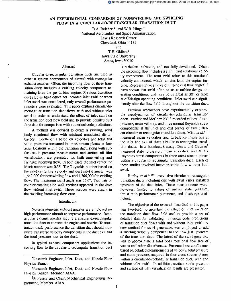
The function of the swirl generator is to producea solid body rotational flow superimposed on a uniform

flow. Ideally, this rotating flow is free of wakes or other

disturbances caused by the mechanism which creates the

rotation. In cylindrical coordinates this velocity field is

described by Eq. (2), where V-centerline is the velocityat the swirl generator centerline and fl is the angularvelocity of the solid body rotation.

V_ = Vcenterline, Ve = fir, Vr = 0 (2)

An example of this flow is represented in Fig. 2. The

swirl angle, ¢, is given by Eq. (3).

0This is the angle of the flow relative to the x-axis mea-

sured by a stationary observer.

Cr C V8

Y

Fig. 2 Solid body rotational flowsuperimposed on uniform flow.

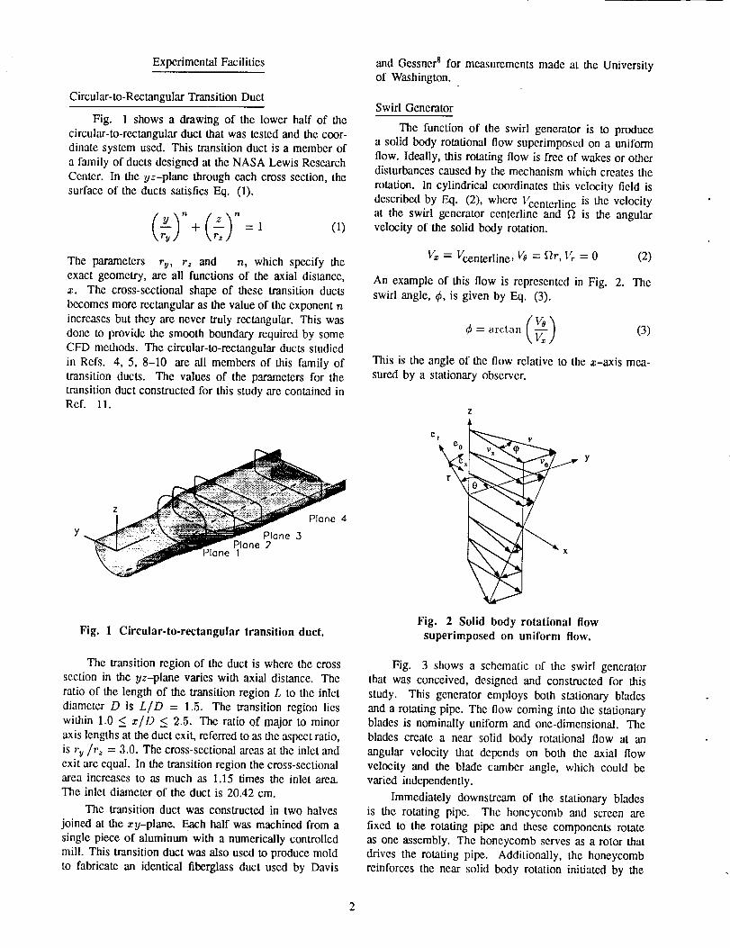
Fig. 3 shows a schematic of the swirl generator

that was conceived, designed and constructed for this

study. This generator employs both stationary blades

and a rotating pipe. The flow coming into the stationaryblades is nominally uniform and one-dimensional. The

blades create a near solid body rotational flow at an

angular velocity that depends on both the axial flow

velocity and the blade camber angle, which could be

varied independently.

Immediately downstream of the stationary bladesis the rotating pipe. The honeycomb and screen are

fixed to the rotating pipe and these components rotate

as one assembly. The honeycomb serves as a rotor that

drives the rotating pipe. Additionally, the honeycomb

reinforces the near solid body rotation initiated by the

Stationary blades

Rotating pipe

WAir flow

"<'--- Honeycomb and screen

Fig. 3 Swirl generator schematic.

stationary blades and dissipates the wakes created by

the stationary blades. A screen is located downstream

of the honeycomb to dissipate the wakes formed by the

honeycomb. The final section of the swirl generator is

the stationary exit section. This section functions as a

stationary component to which the transition duct maybe attached.

The maximum ideal swirl angle Cmax represents the

swirl angle at the rotating pipe wall (r = R) excluding

the boundary layer deceleration of the axial velocity com-

ponent, and is given by Eq. (4). For the results presented

in this paper Cmax = 15.6". Additional details about the

swirl generator design, construction, operation and per-formance are contained in Ref. 11.

Cmax = arctan Vcenterline (4)

Test Facility

The tests were conducted at the NASA Lewis Re-

search Center using the Internal Fluid Mechanics Facil-

ity. This facility was designed to support research on

a variety of internal flow configurations. Air could be

supplied from either the test cell or from a continuous

source of pressurized air. After passing through a large

settling chamber containing honeycomb and screens the

flow proceeds through an axisymmetric contraction hav-

ing an area ratio of 57:1. The flow passes from the con-

traction through either a straight pipe to provide a non-swirling uniform incoming flow to the transition duct, or

the swirl generator to provide a swirling incoming flow.After passing through the transition duct the flow is ex-

hausted into a discharge plenum which is continuously

evacuated by central exhauster facilities.

Experimental Methods and Results

All the results presented in this section are nondi-

mensional. Total and static pressures are presented as

pressure coefficients, having been nondimensionalized as

indicated in Eqs. (5) and (6). Velocity vectors were di-

vided by the local sonic velocity c to yield a Mach vector

and then normalized by the centerline Mach number, as

shown in Eq. (7). Bold type in Eq. (7) indicates vectorquantities. In Eqs. (5) through (7) the reference vari-

ables, subscript_l centerline (r = 0) or wall (r = R),

were evaluated at a location one radius upstream of the

transition duct inlet (x/D = -0.5). This location repre-

sents conditions at the exit of the straight pipe or swirl

generator or the inlet of the transition duct. A discussion

and an analysis of the results are given in the followingsection tiffed Discussion and Conclusions.

p_ = Pc,- Pwall (5)P0,centerline - Pwall

p, = P - Pwall (6)P0,centerline- Pwall

M* - V/c

Mcenterline(7)

Test Conditions

Test conditions were verified by a survey of the flow

field one radius upstream of the transition duct inlet.The test conditions for the flow without and with inlet

swirl are summarized in Table 1. The Reynolds number

is based on the centerline velocity and the transition

duct inlet diameter. The difference in Reynolds number

between the two cases resulted from a total pressure loss

associated with the swirl generator. The boundary layer

thickness 60.,._, displacement thickness 6", momentum

thickness 0, and shape factor H, were calculated from

the survey data. The total temperature for all tests wasnominally 274 K.

Table 1 Test conditions for flow

without and with inlet swirl

Without With inlet

inlet swirl swirl

Mcenterline 0.35 0.35

ReD 1,547,000 1,366,000

Cmax 0.0 ° 15.6°

60.:_5/R (x 100) 8.014 20.484

6*/R (x 100) 1.487 4.048

O/R (x 100) 1.034 2.370

H 1.438 1.707

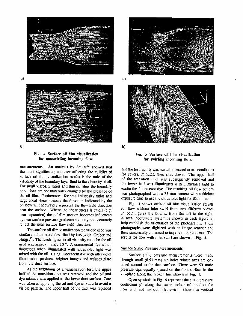
Surface Oil Film Visualization

A surface oil film visualization technique was used

to obtain preliminary information about the flow field nearthe surface Of the transition duct. The results of this initial

"quick look" were used to guide subsequent aerodynamic

a)

b)

Fig. 4 Surface oil film visualization

for nonswirling incoming flow.

measurements. An analysis by Squire 12 showed that

the most significant parameter affecting the validity ofsurface oil film visualization results is the ratio of the

viscosity of the boundary layer fluid to the viscosity ofoil.

For small viscosity ratios and thin oil films the boundary

conditions are not materially changed by the presence of

the oil film. Furthermore, for small viscosity ratios and

large local shear stresses the direction indicated by theoil flow will accurately represent the flow field direction

near the surface. Where the shear stress is small (e.g.

near separation) the oil film motion becomes influenced

by near surface pressure gradients and may not accuratelyreflect the near surface flow field direction.

The surface oil film visualization technique used wassimilar to the method described by Jurkovich, Greber and

Hingst 13. The resulting air to oil viscosity ratio for the oil

used was approximately 10 -6. A commercial dye which

fluoresces when illuminated with ultraviolet light was

mixed with the oil. Using fluorescent dye with ultraviolet

illumination produces brighter images and reduces glarefrom the duct surface.

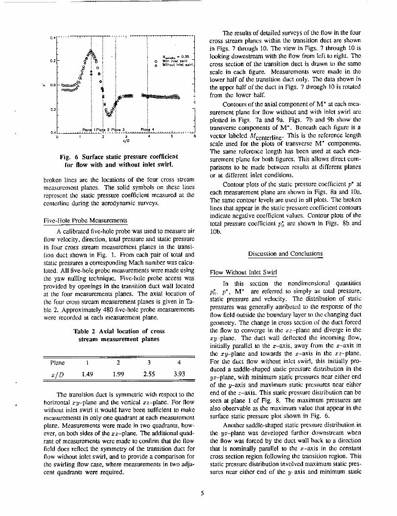
At the beginning of a visualization test, the upperhalf of the transition duct was removed and the oil and

dye mixture was applied to the lower duct surface. Care

was taken in applying the oil and dye mixture to avoid a

visible pattern. The upper half of the duct was replaced

a)

h)

Fig. 5 Surface oil film visualization

for swirling incoming flow.

and the test facility was started, operated at test conditions

for several minutes, then shut down. The upper half

of the transition duct was subsequently removed and

the lower half was illuminated with ultraviolet light to

excite the fluorescent dye. The resulting oil flow pattern

was photographed with a 35 mm camera with sufficient

exposure time to use the ultraviolet light for illumination.

Fig. 4 shows surface oil film visualization resultsfor flow without inlet swirl from two different views.

In both figures the flow is from the left to the right.

A local coordinate system is shown in each figure to

help establish the orientation of the photographs. These

photographs were digitized with an image scanner and

then numerically enhanced to improve their contrast. The

results for flow with inlet swirl are shown in Fig. 5.

Surface Static Pressure Measurements

Surface static pressure measurements were made

through small (0.51 mm) tap holes whose axes are ori-ented normal to the duct surface. There were 50 static

pressure taps equally spaced on the duct surface in the

zz-plane along the broken line shown in Fig. 1.

Open symbols in Fig. 6 represent the static pressure

coefficient p* along the lower surface of the duct forflow with and without inlet swirl. Shown as vertical

4

0.4

0+2

"eL 0,0

-0.2

-0,4

&G5

A: 0

:+Oi

't

_..._.._,,,, - 0.35

0 With _nlot swirl '

A W;thout Tniet mwirl

Plon"; I PlOli,ll ) Pl_n, _I • ,P,l,_? ,4 ......... i .... i ......... _,,,i , ........ ],

1 2 3 4 5

x/O

Fig. 6 Surface static pressure coefficientfor flow with and without inlet swirl.

broken lines are the locations of the four cross stream

measurement planes. The solid symbols on these lines

represent the static pressure coefficient measured at the

centerline during the aerodynamic surveys.

Five-Hole Probe Measurements

A calibrated five-hole probe was used to measure air

flow velocity, direction, total pressure and static pressure

in four cross stream measurement planes in the transi-

tion duct shown in Fig. 1. From each pair of total and

static pressures a corresponding Mach number was calcu-

lated. All five-hole probe measurements were made using

the yaw nulling technique. Five-hole probe access was

provided by openings in the transition duct wall located

at the four measurements planes. The axial location of

the four cross stream measurement planes is given in Ta-

ble 2. Approximately 480 five-hole probe measurements

were recorded at each measurement plane.

Table 2 Axial location of cross

stream measurement planes

Plane 1 2 3 4

x/D 1.49 1.99 2.55 3.93

The transition duct is symmetric with respect to the

horizontal xy-plane and the vertical xz-plane. For flowwithout inlet swirl it would have been sufficient to make

measurements in only one quadrant at each measurement

plane. Measurements were made in two quadrants, how-

ever, on both sides of the xz-plane. The additional quad-rant of measurements were made to confirm that the flow

field does reflect the symmetry of the transition duct for

flow without inlet swirl, and to provide a comparison for

the swirling flow case, where measurements in two adja-

cent quadrants were required.

The results of detailed surveys of the flow in the four

cross stream planes within the transition duct are shownin Figs. 7 through 10. The view in Figs. 7 through 10 is

looking downstream with the flow from left to right. Thecross section of the transition duct is drawn to the same

scale in each figure. Measurements were made in thelower half of the transition duct only. The data shown in

the upper half of the duct in Figs. 7 through 10 is rotatedfrom the lower half.

Contours of the axial component of M* at each mea-

surement plane for flow without and with inlet swirl are

plotted in Figs. 7a and 9a. Figs. 7b and 9b show the

transverse components of M*. Beneath each figure is a

vector labeled Mcenterline. This is the reference lengthscale used for the plots of transverse M* components.

The same reference length has been used at each mea-

surement plane for both figures. This allows direct com-

parisons to be made between results at different planesor at different inlet conditions.

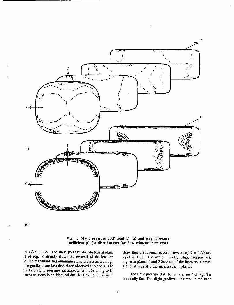
Contour plots of the static pressure coefficient p* at

each measurement plane are shown in Figs. 8a and 10a.

The same contour levels are used in all plots. The broken

lines that appear in the static pressure coefficient contours

indicate negative coefficient values. Contour plots of the

total pressure coefficient p(*_are shown in Figs. 8b and10b.

Discussion and Conclusions

Flow Without Inlet Swirl

In this section the nondimensional quantities

p_, p*, M* are referred to simply as total pressure,

static pressure and velocity. The distribution of static

pressures was generally attributed to the response of theflow field outside the boundary layer to the changing duct

geometry. The change in cross section of the duct forcedthe flow to converge in the xz-plane and diverge in the

xy-plane. The duct wall deflected the incoming flow,

initially parallel to the x-axis, away from the z-axis in

the xy-plane and towards the x-axis in the xz-plane.

For the duct flow without inlet swirl, this initially pro-

duced a saddle-shaped static pressure distribution in the

yz-plane, with minimum static pressures near either end

of the y-axis and maximum static pressures near either

end of the z-axis. This static pressure distribution can be

seen at plane 1 of Fig. 8. The maximum pressures are

also observable as the maximum value that appear in the

surface static pressure plot shown in Fig. 6.

Another saddle-shaped static pressure distribution in

the yz-plane was developed further downstream when

the flow was forced by the duct wall back to a direction

that is nominally parallel to the x-axis in the constant

cross section region following the transition region. This

static pressure distribution involved maximum static pres-

sures near either end of the y-axis and minimum static

5

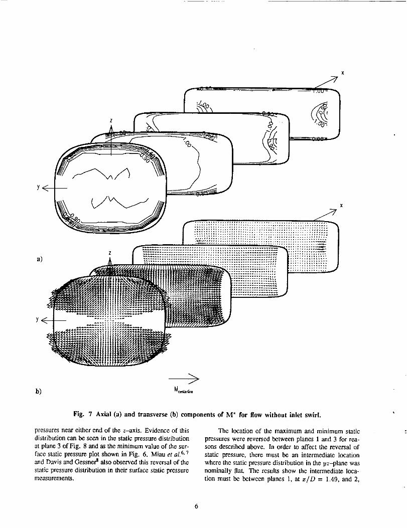
a)

b)

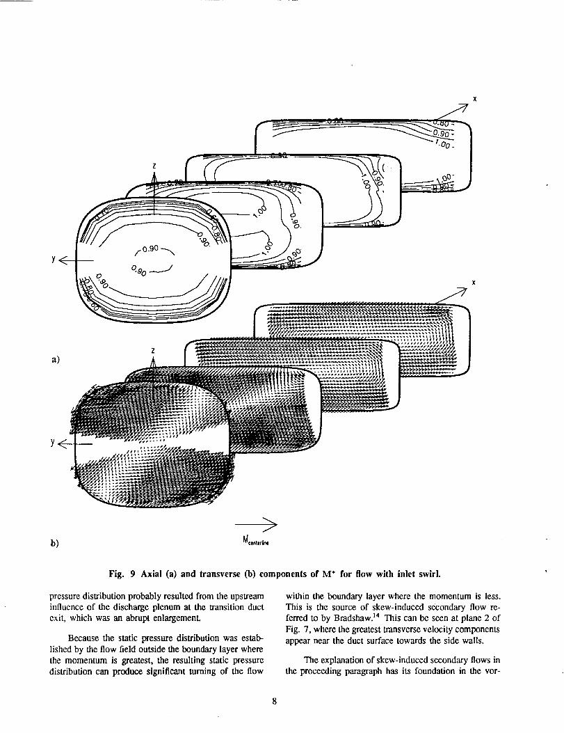
Fig. 7 Axial (a) and transverse (b) components of M* for flow without inlet swirl.

pressures near either end of the z-axis. Evidence of this

distribution can be seen in the static pressure distribution

at plane 3 of Fig. 8 and as the minimum value of the sur-

face static pressure plot shown in Fig. 6. Miau et al. 6, 7and Davis and Gessner s also observed this reversal of the

static pressure distribution in their surface static pressuremeasurements.

The location of the maximum and minimum static

pressures were reversed between planes 1 and 3 for rea-sons described above. In order to affect the reversal of

static pressure, there must be an intermediate location

where the static pressure distribution in the yz-plane was

nominally flat. The results show the intermediate loca-

tion must be between planes 1, at z/D = 1.49, and 2,

Y<

a)

_S/

L.

b)

Fig. 8 Static pressure coefficient p* (a) and total pressurecoefficient pq_ (b) distributions for flow without inlet swirl.

at x/D = 1.99. The static pressure distribution at plane2 of Fig. 8 already shows the reversal of the location

of the maximum and minimum static pressures, althoughthe gradients are less than those observed at plane 3. The

surface static pressure measurements made along axial

cross sections in an identical duct by Davis and Gessner 8

show that the reversal occurs between x/D = 1.60 and

x/D = 1.90. The overall level of static pressure washigher at planes 1 and 2 because of the increase in cross-

sectional area at these measurement planes.

The static pressure distribution at plane 4 of Fig. 8 is

nominally fiat. The slight gradients observed in the static

a)

b) _(centerl_

Fig. 9 Axial (a) and transverse (b) components of M* for flow with inlet swirl.

pressure distribution probably resulted from the upstreaminfluence of the discharge plenum at the transition ductexit, which was an abrupt enlargement.

Because the static pressure distribution was estab-lished by the flow field outside the boundary layer wherethe momentum is greatest, the resulting static pressuredistribution can produce significant turning of the flow

within the boundary layer where the momentum is less.This is the source of skew-induced secondary flow re-ferred to by Bradshaw} 4 This can be seen at plane 2 of

Fig. 7, where the greatest transverse velocity componentsappear near the duct surface towards the side walls.

The explanation of skew-induced secondary flows inthe proceeding paragraph has its foundation in the vor-

a)

\0.9(

b)

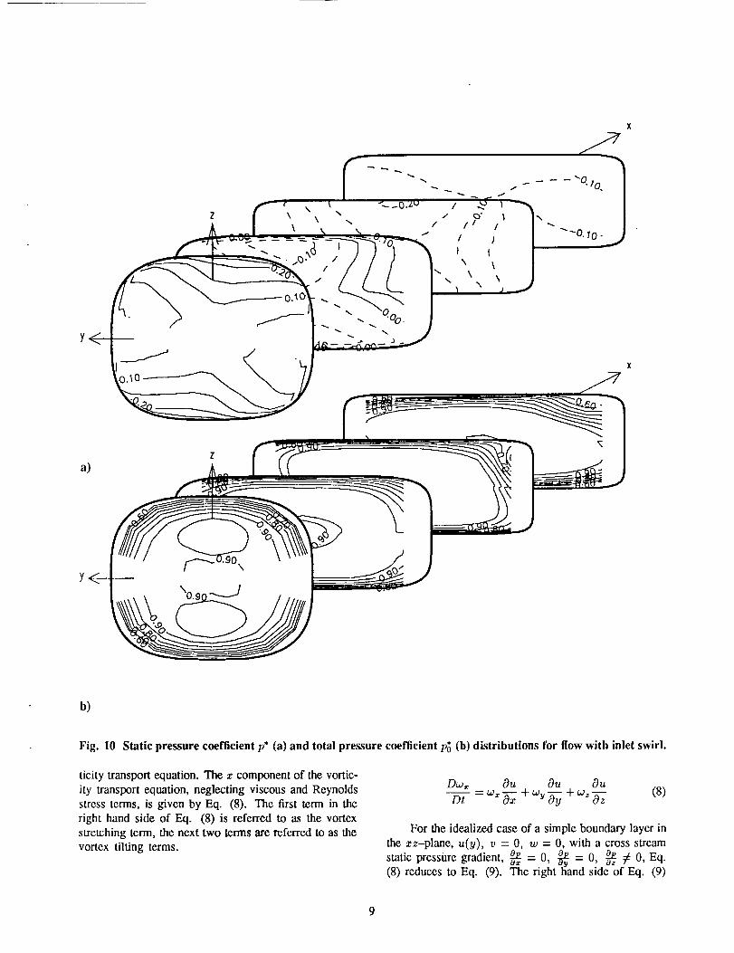
Fig. 10 Static pressure coefficient p* (a) and total pressure coefficient p_ (b) distributions for flow with inlet swirl.

ticity transport equation. The x component of the vortic-ity transport equation, neglecting viscous and Reynoldsstress terms, is given by Eq. (8). The first term in theright hand side of Eq. (8) is referred to as the vortexstretching term, the next two terms are referred to as thevortex tilting terms.

D_o_ Ou Ou Ou

Dt - w_ O--z+ wy _ + wz _ (8)

For the idealized case of a simple boundary layer in

the zz-plane, u(y), v = O, w = O, with a cross streamstatic pressure gradient, op = n o_z =(8) reduces to Eq. (9). "_e right _and 0, _ :/: 0, Eq.side of Eq. (9)

9

X

_centerl_ne

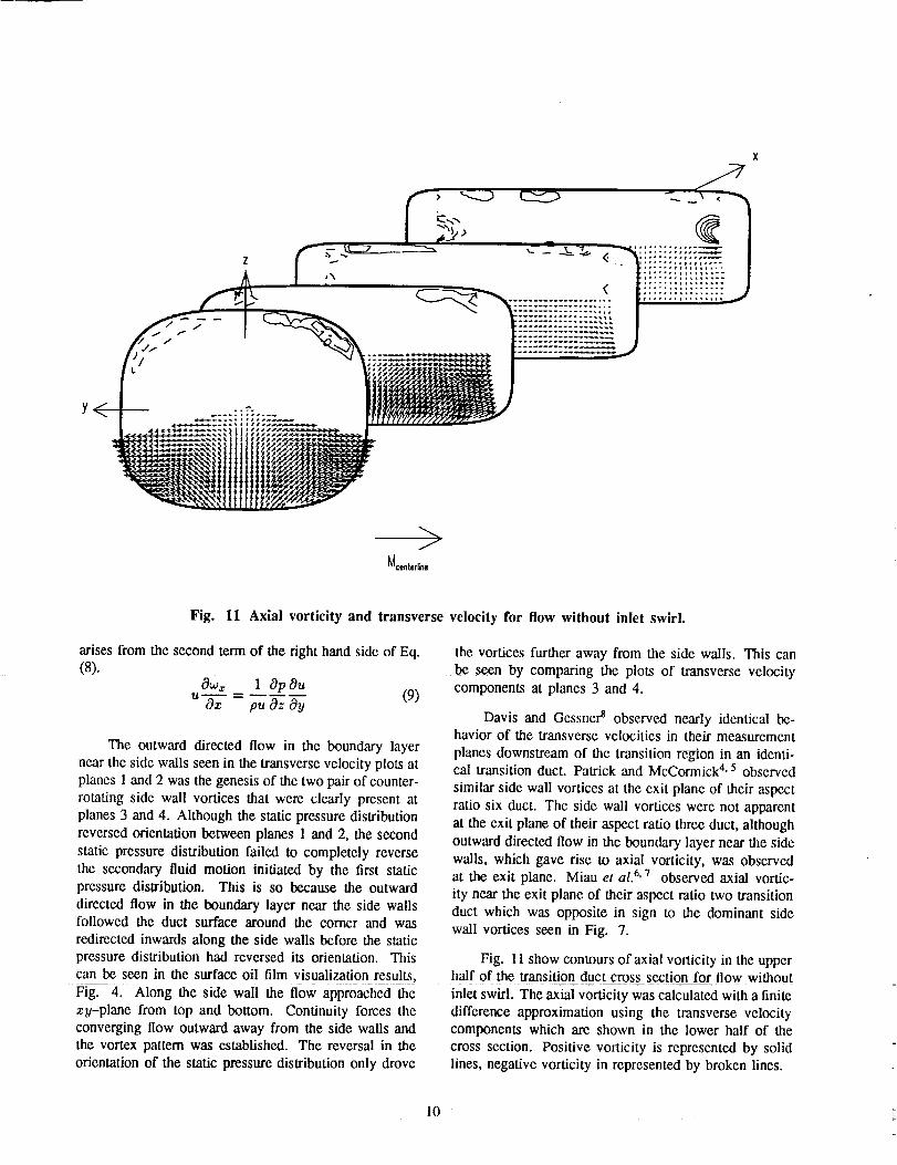
Fig. lI Axial vorticity and transverse velocity for flow without inlet swirl.

arises from the second term of the right hand side of Eq.(8).

8w_ 1 8p Ou

u--_-z = pu Oz ay (9)

The outward directed flow in the botmdary layer

near the side walls seen in the transverse velocity plots atplanes 1 and 2 was the genesis of the two pair of counter-

rotating side wall vortices that were clearly present at

planes 3 and 4. Although the static pressure distribution

reversed orientation between planes 1 and 2, the second

static pressure distribution failed to completely reverse

the secondary fluid motion initiated by the first staticpressure distribution. This is so because the outward

directed flow in the boundary layer near the side wallsfollowed the duct surface around the comer and was

redirected inwards along the side walls before the static

pressure distribution had reversed its orientation. This

the vortices further away from the side walls. This can

be seen by comparing the plots of transverse velocity

components at planes 3 and 4.

Davis and Gessner s observed nearly identical be-havior of the transverse velocities in their measurement

planes downstream of the transition region in an identi-cal transition duct. Patrick and McCormick 4. 5 observed

similar side wall vortices at the exit plane of their aspect

ratio six duct. The side wall vortices were not apparent

at the exit plane of their aspect ratio three duct, although

outward directed flow in the boundary layer near the side

walls, which gave rise to axial vorticity, was observedat the exit plane. Miau et al. 6"7 observed axial vortic-

ity near the exit plane of their aspect ratio two transition

duct which was opposite in sign to the dominant side

wall vortices seen in Fig. 7.

Fig. 11 show contours of axial vorticity in the uppercan be seen in the surface oil film visualization results, half of the transition duct cross section for flow without

Fig. 4. Along the side wall the flow approached the inlet swirl. The axial vorticity was calculated with a finite

zy-plane from top and bottom. Continuity forces the difference approximation using the transverse velocityconverging flow outward away from the side walls and components which are shown in the lower half of the

the vortex pattern was established. The reversal in the cross section. Positive vorticity is represented by solidorientation of the static pressure distribution only drove lines, negative vorticity in represented by broken lines.

10

Atplane1of Fig.I 1 theinitiationofthesidewallvorticescanbeseenin thegenerationof positiveaxialvorticityin theupperrightquadrantandnegativeaxialvorticityin theupperleft quadrant.Thisaxialvorticityresultedfromthestaticpressuregradientdriven,skew-inducedsecondaryflowin theboundarylayer,asex-plainedearlier.Thesignof theaxialvorticityshownin Fig. 11iscorrectlypredictedby Eq. (9). At plane2 of Fig. 11convectionhadcarriedtheaxialvortic-ity outwardstowardsthesidewalls.Atplane3of Fig.11convectionhadcarriedtheaxialvorticityobservedatplane1tothesidewallsandoutof themeasurementre-gion.Thenewstaticpressuredistribution,however,hadgeneratedaxialvorticitywhichis oppositeinsignfromtheaxialvorticityobservedat plane1. Thisprovidesadditionalevidencethatthesecondstaticpressuredistri-butiondoesn'tsimplyeliminatetheaxialvorticitycreatedbythefirststaticpressuredistributionbecauseconvectionhadcarriedthevorticityobservedatplane1awayfromtheregionwheretheoppositesignedaxialvorticityispro-duced.Atplane4ofFig.11theaxialvorticityobservedat planeI is nowreadilyapparentnearthesidewalls,whilethemuchweakeroppositesignedaxialvorticityhasremainedinnearlythesamelocationasobservedatplane3.

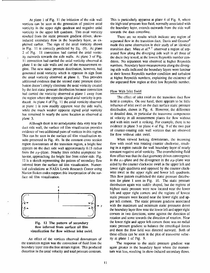
Althoughthereisnoaerodynamicdataveryneartheductsidewall,thesurfaceoil filmvisualizationprovidesevidenceoftwoadditionalpairsof vorticesinthisregion.Thiscanbeseenin thesurfaceoil filmvisualizationre-sultspresentedinFig. 4b. In theconstantcrosssectionregiondownstreamof thetransitionregion,abrightlineappearsontheductsidewallapproximately0.15radiusfromthezy-plane. Nearby lines exhibit asymptotic be-

havior, approaching the bright line from either side. Fig.

12 is a sketch representing the pattern of secondary flowinferred from the surface oil film visualization. Numer-

ical calculations at NASA Lewis Research Center using

Navier-Stokes codes support this interpretation of the sur-face oil film visualization.

Fig. 12 The pattern of secondaryflow inferred from surface oil film

visualization for flow without inlet swirl.

An effect of the vortices observed downstream of

the transition region was the convection of fluid from the

boundary layer into the free stream region. This produced

distortion in the axial velocity and total pressure contours.

This is particularly apparent at plane 4 of Fig. 8, where

the high total pressure loss fluid, normally associated withthe boundary layer, extends outwards from the side walltowards the duct centerline.

There are no results which indicate any region ofseparated flow in the transition duct. Davis and Gessner 8

made this same observation in their study of an identical

transition duct. Miau et al. 6' 7 observed a region of sep-

arated flow along the diverging side wall in all three of

the ducts they tested, at the lowest Reynolds number con-

dition. No separation was observed at higher Reynoldsnumbers. Boundary layer measurements along the diverg-

ing side walls indicated the boundary layers were laminar

at their lowest Reynolds number condition and turbulent

at higher Reynolds numbers, explaining the existence of

the separated flow region at their low Reynolds number.

Flow With Inlet Swirl

The effect of inlet swirl on the transition duct flow

field is complex. On one hand, there appears to be little

influence of inlet swirl on the duct surface static pressure

distribution, shown in Fig. 6. However, the difference

in detailed data, in particular the transverse components

of velocity in all measurement planes for flow without

and with inlet swirl is striking. For example, there is no

evidence in plane 3 or plane 4 of Fig. 9 of the two pair

of counter-rotating side wall vortices that are observedfor flow without inlet swirl.

When viewed looking downstream, the incoming

flow with swirl was rotating counter clockwise, result-

ing in a region outside the wall boundary layer of nearly

constant negative axial vorticity. The overwhehning fluid

flow effect was that the duct geometry driven convergence

in the zz-plane and the divergence in the zy-plane was

aided by the counter clockwise swirl in the upper left and

lower right quadrants and opposed by the counter clock-

wise swirl in the upper right and lower left quadrants.

This flow pattern established the static pressure distribu-

tion for plane 1 seen in Fig. 10. The static pressure

distribution again was saddle shaped, but the regions of

highest static pressure were now located near the lower

left and upper right comers and the regions of lowest

static pressure were located near the lower right and up-

per left comers. The static pressure gradient associated

with the maximum and minimum static pressures drove

the boundary layer flow near the lower left and upper right

comers in two directions, some against the direction ofrotation and some towards the direction of rotation. Near

the lower right and upper left comers there was no radial

static pressure gradient to balance the centrifugal forcesand there the flow field was directed outward. Both of

these effects can be seen in the plot of transverse veloc-

ity at plane 1 of Fig. 9.

The response to the static pressure gradient was

again greater in the boundary layer where the momen-

tum was less, resulting in skew-induced secondary flows.

11

X

\

_centerllrN_

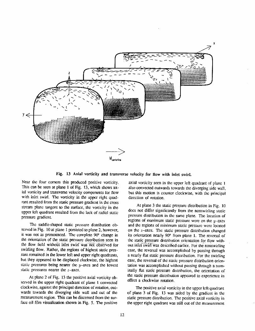
Fig.

Near the four corners this produced positive vorticity.

This can be seen at plane 1 of Fig. 13, which shows ax-

ial vorticity and transverse velocity components for flow

with inlet swirl The vorticity in the upper right quad-

rant resulted from the static pressure gradient in the cross

stream plane tangent to the surface, the vorticity in theupper left quadrant resulted from the lack of radial static

pressure gradient.

The saddle-shaped static pressure distribution ob-

served in Fig. 10 at plane 1 persisted to plane 2, however,

it was not as pronounced. The complete 90 ° change inthe orientation of the static pressure distribution seen inthe flow field without inlet swirl was not observed for

swirling flow. Rather, the regions of highest static pres-

sure remained in the lower left and upper right quadrants,

but they appeared to be displaced clockwise, the highest

static pressures being nearer the y-axes and the loweststatic pressures nearer the z-axes.

At plane 2 of Fig. 13 the positive axial vorticity ob-served in the upper right quadrant of plane 1 convected

clockwise, against the principal direction of rotation, out-

wards towards the diverging side wall and out of the

measurement region. This can be discerned from the sur-

face oil film visualization shown in Fig. 5. The positive

13 Axial vorticity and transverse velocity for flow with inlet swirl.

axial vorticity seen in the upper left quadrant of plane 1

also convected outwards towards the diverging side wail,

but this motion is counter clockwise, with the principaldirection of rotation.

At plane 3 the static pressure distribution in Fig. 10

does not differ significantly from the nonswirling static

pressure distribution in the sanae plane. The location of

regions of maximum static pressure were on the y-axesand the regions of minimum static pressure were located

on the z-axes. The static pressure distribution changedits orientation nearly 90 ° from plane 1. The reversal of

the static pressure distribution orientation for flow with-

out inlet swirl was described earlier. For the nonswirling

case, the reversal was accomplished by passing through

a nearly fiat static pressure distribution. For the swirlingcase, the reversal of the static pressure distribution orien-

tation was accomplished without passing through a nom-inally fiat static pressure distribution, the orientation of

the static pressure distribution appeared to experience ineffect a clockwise rotation.

The positive axial vorticity in the upper left quadrant

of plane 3 of Fig. 13 was aided by the gradient in the

static pressure distribution. The positive axial vorticity in

the upper right quadrant was still out of the measurement

12

region. Thisaxialvorticitywasnotaffectedby thegradientin thestaticpressuredistributionbecauseof itslocation.

Thestaticpressuredistributionshowninplane4ofFig.10hadthesameshapeasthedistributioninplane3,however,thegradientswerenotasgreat.Atthislocationandfurtherdownstream,thestaticpressuredistributionhadlittleeffectontheboundarylayerflow.

Positiveaxialvorticityis presentin eachcomeratplane4 of Fig. 13. Thiswasthesamepositiveaxialvorticitygeneratedin eachrespectivequadrantin plane1. Thepositivevorticityin theupperleftquadrantwasobservedin all fourmeasurementplanes.Thepositivevorticityin theupperrightquadrantwasseenat plane1,buthadconvectedoutof themeasurementregionatplanes2 and3, andreappearedatplane4.

Thedistortionof totalpressureis mostapparentintheupperrightandlowerleftquadrantinplanes3 and4 ofFig. 10.Asin thenonswirlingcase,thisdistortionresultedfromtheconvectionof boundarylayerfluidbysecondaryflows.Theslightdepressionin totalpressurenearthecenterlinethatappearedinall fourplanesisanartifactof theswirlgenerator.All measurementsindicatethattheflowremainedattachedthroughoutthetransitionduct.

Summary

When utilized as exhaust system components of

aircraft with rectangular nozzles, the incoming flow to

circular-to-rectangular transition ducts often includes a

swirling velocity component remaining from the gas tur-

bine engine. Inlet swirl significantly changes the tran-sition duct flow field. Outside the boundary layer, the

response of the flow field velocity to the changing duct

geometry gives rise to the static pressure distribution. For

nonswirling incoming flow the static pressure distribu-

tion produced skew-induced secondary flows within the

boundary layer which evolved into two pair of counter-

rotating side wall vortices. For the inlet swirl case stud-ied the side wall vortices were not observed. The static

pressure distribution was altered by the swirling velocityflow field to an extent that the side wall vortices were

suppressed. The effects of inlet swirl should be included

in the design of circular-to-rectangular transition ducts

for aircraft exhaust systems.

References

1Whitney, W. J., Schum, H. J., and Behning, F. P., "Cold-

Air Investigation of a Turbine for High-Temperature-

Engine Application IV - Two-Stage Turbine Perfor-

mance," NASA TN D-6960, 1972.

2 Szanca, E. M., Schum, H. J., and Hotz, G. M., "Research

Turbine for High-Temperature Core Engine Application I- Cold-Air Over_l Performance of Solid Scaled Turbine,"

NASA TN D-7557, 1974.

3 Schwab, J. R., Stabe, R. G., and Whitney, W. J.,

"Analytical and Experimental Study of Flow Through

Axial Turbine Stage With a Nonuniform Inlet Radial

Temperature Profile," AIAA Paper 83-1175, 1983.

4Patrick, W. P. and McCormick, D. C., "Laser Ve-locimeter and Total Pressure Measurements in Circular-

to-Rectangular Transition Ducts," United Technologies

Research Center Report 87-41, June 1988. NASA CR

to be published.

Spatrick, W. P. and McCormick, D. C., "Circular-to-

Rectangular Duct Flows - A Benchmark Experimental

Study," Society of Automotive Engineers Tech. Rep.

871776, 1988.

6Miau, J. J., Lin, S. A., Chou, J. H., Wei, C. Y.,

and Lin, C. K., "An Experimental Study of Flow in a

Circular-Rectangular Transition Duct," AIAA Paper 88-3029, 1988.

7Miau, J. J., Leu, T. S., Chou, J. H., Lin, S. A., and

Lin, C. K., "Flow Distortion in a Circular-to-Rectangular

Transition Duct," AIAA Journal, Vol. 28, Aug. 1990,

pp. 1447-1456.

8Davis, D. O. and Gessner, F. B., "Experimental In-

vestigation of Turbulent Flow Through a Circular-to-

Rectangular Transition Duct," AIAA Paper 90-1505,1990.

9j. R. Burley, J. and Carlson, J. R., "Circular-to-

Rectangular Transition Ducts for High-Aspect Ratio Non-axisymmetric Nozzles," AIAA Paper 85-1346, 1985.

t0j. R. Burley, J., Bangert, L. S., and Carlson,

J. R., "Investigation of Circular-to-Rectangular Transition

Ducts for High-Aspect Ratio Nonaxisymmetric Nozzles,"NASA TP 2534, Mar. 1986.

l lReichert, B. A., A Study of ltigh Speed Flows in

an Aircraft Transition Duct. PhD thesis, Iowa State

University, Ames, Iowa, 1991.

12Squire, L. C., Maltby, R. L., Keating, R. F. A., and

Stanbrook, A., "The Surface Oil Flow Technique," in

Flow Visualization in Wind Tunnels Using Indicators

(Maltby, R. L., ed.), pp. 1-28, AGARD, Apr. 1962.

AGARDograph 70.

13Jurkovich, M. S., Greber, I., and Hingst, W. R., "Flow

Visualization Studies of a 3-D Shock/Boundary LayerInteraction in the Presence of a Non-Uniform Approach

Boundary Layer," AIAA Paper 84-1560, 1984.

14Bradshaw, P., "Turbulent Secondary Flows," Annual

Review of Fluid Mechanics, Vol. 19, 1987, pp. 53-74.

13

N/ ANat_al Aeronautics and

Space Administration

Report Documentation Page

1. Report No. NASA TM - 104359 2. Government Accession No. 3. Reciplenfs Catalog No.

AIAA - 91 - 0342

5. Report Date4. Title and Subtitle

An Experimental Comparison of Nonswirling and SwirlingFlow in a Circular-to-Rectangular Transition Duct

7. Author(s)

B.A. Reichert, W.R. Hingst, and T.H. Okiishi

9. Performing Organization Name and Address

National Aeronautics and Space AdministrationLewis Research Center

Cleveland, Ohio 44135 - 3191

t2. Sponsoring Agency Name and Address

National Aeronautics and Space Administration

Washington, D.C. 20546 - 0001

6. Performing Organization Code

8. Performing Organization Report No.

E- 6149

10. Work Unit No.

505 - 62 - 91

11. Contract or Grant No,

13. Type of Report and Period Covered

Technical Memorandum

14. Sponsoring Agency Code

15. Supplementary Notes

Prepared for the 29th Aerospace Sciences Meeting sponsored by the American Institute for Aeronautics and Astronautics,Reno, Nevada, January 7-10, 1991. B.A. Reichert and W.A. Hingst, NASA Lewis Research Center, T.H. Okiishi, IowaState University, Ames, Iowa 50011. Responsible person, B.A. Reichert, (216) 433-8397.

16, Abstract

Circular-to-rectangular transition ducts are used as exhaust system components of aircraft with rectangular exhaust

nozzles. Often, the incoming flow of these transition ducts includes a swirling velocity component remaining from thegas turbine engine. Previous transition duct studies have either not included inlet swirl or when inlet swirl was

considered, only overall performance parameters were evaluated. This paper explores circular-to-rectangular transitionduct flows with and without inlet swirl in order to understand the effect of inlet swirl on the transition duct flow field

and to provide detailed duct flow data for comparison with numerical code predictions. A method was devised tocreate a swirling, solid body rotational flow with minimal associated disturbances. Coefficients based on velocities

and total and static pressures measured in cross stream planes at four axial locations within the transition duct, alongwith surface static pressure measurements and surface oil film visualization, are presented for both nonswirling and

swirling incoming flow. In both cases the inlet centerline Mach number was 0.35. The Reynolds number based on theinlet centerline velocity and duct inlet diameter was 1,547,000 for nonswirling flow and 1,366,000 for swirling flow.

The maximum swirl angle was 15.6". Two pair of counter-rotating side wall vortices appeared in the duct flowwithout inlet swirl. These vortices were absent in the swirling incoming flow case.

t7. Key Words (Suggested by Author(s))

Ducted flow; Rotating fluids; Vorticity; Exhaust systems;

Flow distortions; Secondary flow

18. Distribution Statement

Unclassified - Unlimited

Subject Category 02

19, Security Classif. (of the report) 20. Secudty Classit. (of this page) 21. No. of pages 22. Price"

Unclassified Unclassified 14 A03

NASAFORMle2aOCT86 *For sale bythe NationalTechnicalInformation Service,Springfield,Virginia 22161