HAL Id: hal-01574079https://hal.inria.fr/hal-01574079

Submitted on 11 Aug 2017

HAL is a multi-disciplinary open accessarchive for the deposit and dissemination of sci-entific research documents, whether they are pub-lished or not. The documents may come fromteaching and research institutions in France orabroad, or from public or private research centers.

L’archive ouverte pluridisciplinaire HAL, estdestinée au dépôt et à la diffusion de documentsscientifiques de niveau recherche, publiés ou non,émanant des établissements d’enseignement et derecherche français ou étrangers, des laboratoirespublics ou privés.

An evolutionary scheme for decision tree constructionNour El Islem Karabadji, Hassina Seridi, Fouad Bousetouane, Wajdi Dhifli,

Sabeur Aridhi

To cite this version:Nour El Islem Karabadji, Hassina Seridi, Fouad Bousetouane, Wajdi Dhifli, Sabeur Aridhi. An evolu-tionary scheme for decision tree construction. Knowledge-Based Systems, Elsevier, 2017, 119, pp.166- 177. �10.1016/j.knosys.2016.12.011�. �hal-01574079�

An Evolutionary Scheme for Decision Tree Construction

Nour El Islem Karabadjia,b,⇤, Hassina Seridib, Fouad Bousetouanec, WajdiDhiflid, Sabeur Aridhie

aPreparatory School of Science and Technology, Annaba, P.O. Box 218, 23000, Algeria.bElectronic Document Management Laboratory (LabGED), Badji Mokhtar-Annaba

University, P.O. Box 12 Annaba, Algeria.cReal Time Intelligent System Laboratory, University of Nevada, Las Vegas, NV 89154,

USA.dDepartment of Computer Science, University of Quebec At Montreal, PO box 8888,

Downtown station, Montreal (Quebec) Canada, H3C 3P8.eUniversity of Lorraine, LORIA, Campus Scientifique, BP 239, 54506

Vandoeuvre-les-Nancy, France.

Abstract

Classification is a central task in machine learning and data mining. Deci-sion tree (DT) is one of the most popular learning models in data mining.The performance of a DT in a complex decision problem depends on thee�ciency of its construction. However, obtaining the optimal DT is nota straightforward process. In this paper, we propose a new evolutionarymeta-heuristic optimization based approach for identifying the best settingsduring the construction of a DT. We designed a genetic algorithm coupledwith a multi-task objective function to pull out the optimal DT with thebest parameters. This objective function is based on three main factors: (1)Precision over the test samples, (2) Trust in the construction and validationof a DT using the smallest possible training set and the largest possible test-ing set, and (3) Simplicity in terms of the size of the generated candidateDT, and the used set of attributes. We extensively evaluate our approach on13 benchmark datasets and a fault diagnosis dataset. The results show that

⇤Corresponding author. Address: LabGED, Badji Mokhtar University, PO Box 12,23000, Annaba, Algeria. Tel: 0021338872678; Fax: 0021338872436

Email addresses: karabadji@labged.net (Nour El Islem Karabadji ),seridi@labged.net (Hassina Seridi), fouad.bousetouane@unlv.edu (FouadBousetouane), dhifli.wajdi@courrier.uqam.ca (Wajdi Dhifli),sabeur.aridhi@loria.fr (Sabeur Aridhi)

Preprint submitted to Knowledge-Based Systems December 8, 2016

it outperforms classical DT construction methods in terms of accuracy andsimplicity. They also show that the proposed approach outperforms Ant-Tree-Miner (an evolutionary DT construction approach), Naive Bayes andSupport Vector Machine in terms of accuracy and F-measure.

Keywords: Decision Trees, Genetic Algorithms, Attributes Selection, DataReduction.

1. Introduction

Data Mining is the process of extracting information and knowledge fromhuge datasets. Classification is one of the most popular tasks in data mining.It involves building a classification model (classifier) based on a training setof labeled examples, where the generated classifier should be able to classifynew instances properly. In general, the training examples are labeled by anexpert or based on some experimental results (e.g., weather observations).The classifier is supposed to discover significant and hidden patterns overthe training data that allow it to predict the labels/classes of new instancese�ciently. Technically, the classification model is parameterized accordingto the characteristics of the training examples. However, several modelscould be estimated for the same training set. Obtaining the model withthe highest precision and generalization capabilities is not trivial. Indeed, itrelies on finding the optimal model h⇤(x) that best minimizes the loss (crossentropy loss, hinge loss, etc.) between the predicted labels and the groundtruth for examples of an evaluation set.

In the literature, a wide spectrum of di↵erent classification approacheswas developed such as support vector machines [16, 24], bayesian inferencebased approaches [1, 33], neural networks [26, 34] and deep learning [32,44]. In contrast of these popular approaches, decision trees (DTs) are stillpreferred for a wide range of data mining problems. This is due to the factthat they encode explicitly semantic relationships between attributes whichallow users to understand easily the behavior of the generated models.

The construction of a DT is mainly based on two stages: (1) a growingphase and (2) a pruning phase. The growing phase is the process of split-ting the training data repeatedly into two or more subsets in a hierarchicalmanner. Di↵erent algorithms could be used in this stage which involves dif-ferent growing strategies such as Gini and �2. The growing process stopsonce stopping criteria are satisfied or all instances of each subset wrap the

2

same class. In general, the growing stage outputs very large-depth DTs withhigh complexity.

In the pruning phase, di↵erent heuristic strategies are often used to re-duce the size and complexity of the constructed DT [9, 38, 42, 43]. In fact,the pruning also allows to prevent over-fitting by removing all sections of theDT that might be a↵ected by noisy or imprecise data. However, finding thebest trade-o↵ between the pruning level and the prediction accuracy of theDT over the test samples is not an easy task. Since an over-pruning makesa distortion of the classification model and the latter will only represent asmall portion of the training set. This engenders an over-generalization ofthe classification model and the latter will accept many false positives inthe prediction. An under-pruning makes the classification model overfitsthe training data. Generating an accurate and optimized DT for a com-plex dataset (e.g., non-linearly separable) requires answering the followingquestions:

• How to choose the most appropriate training samples?

• What are the model parameters that fit better the learning data?

• What are the set of attributes to be considered?

• When to stop the growing phase?

• When to stop the pruning phase?

Choosing a pruning technique for a specific decision problem (e.g., ID3[30]) is not straightforward and there is no formal justification about thechoice of the DT construction technique. If all those questions have to besimultaneously answered, a very complex combinatorial problem must besolved, which evolves exponentially in terms of memory consumption andcomputation time. Meta-heuristic strategies are known as powerful searchalgorithms (Genetic Algorithm (GA), Particle Swarm Optimization, etc.) forfinding the optimal solution for complex combinatorial problems.

In this paper, we present a new powerful approach for optimal DT con-struction with high accuracy for complex classification/prediction problems.This approach is mainly based on a genetic algorithm that allows findingthe optimal DT by taking into account several combinations of the possi-ble parameters, subsets of attributes, and subsets of training/testing exam-ples. Experimental results show that our approach outperforms ordinary

3

DT construction approaches in terms of prediction accuracy and complex-ity of the constructed DT model. These results also illustrate a competitivebehaviour of our approach with a large magnitude in term of accuracy and F-measure compared to known well established classifiers namely Naive Bayesand Support Vector Machine. In addition, the accuracy and runtime resultsof the proposed approach have shown good performances compared to an antcolony optimisation algorithm denoted Ant-Tree-Miner [39] that constructsimproved DTs. To summarize, the identified contributions of this work areas follow:

- We propose a GA scheme to deal with a range of key strategic choicesto improve the accuracy and the simplicity of the DT. To this end,the best chromosome that allows the construction of an optimal DT isselected.

- We design a multi-task fitness function that allows to pull out the mostappropriate chromosome according to a set of multiple constraints.These constraints consist of (1) Favoring the improvement of the ac-curacy of the DT. (2) Reducing the size of the used sets of attributesand training samples, as well as the size of the constructed DT. (3)Increasing the size of the set of testing samples.

- We experimentally evaluate the performance of our approach on variousbenchmark datasets and we show that it outperforms multiple ordinaryDT construction approaches, Naive Bayes and SVM classifiers, andAnt-Tree-Miner.

Our approach can be used in a variety of real-world classification prob-lems where the choice of the best combination of the possible parameters,subsets of attributes, and subsets of training/testing examples is hard. Forinstance, in protein sequence and structure annotation, classification modelsare one of most useful techniques to predict the annotation of un-annotatedproteins [18, 2]. Mainly, the task is to predict the structural or functionalclass for each protein based on a set of discriminative patterns (e.g. subse-quences or substructures) used as attributes and with respect to a referencedataset of known labeled proteins. The problem is that the size of the ref-erence database in real-world cases is usually extremely large (for instanceUniprot [15] counts more than 80 million sequences) making straightforwardapplication of exact classification algorithms extremely costly or even unfea-sible. Besides the number of patterns used as attributes could be very high

4

making the classification task even harder due to the curse of dimensionality[19]. Our approach is highly useful in such cases as it allows to build a simpleand e�cient DT model by pulling out automatically the best subsets of ref-erence training and test samples as well as the best subset of attributes andparameters. Another domain of application of our approach is recommenda-tion systems which are among the most important tools in many real-worldapplications such as social networks like Facebook, commercial websites likeAmazon, streaming media and video websites like Netflix, etc. In this do-main of application the system is interested in recommending for each usernovel profiles, items or products that could interest him and thus increasethe business income. The recommendation is usually based on the similaritybetween the user of interest and a subset of the most similar users selectedfrom a reference database [6]. The bottleneck here is that the size of the ref-erence database is usually huge thus making the search extremely costly andeven sometimes unfeasible. Besides, the number of items and ratings at eachprofile could also be very large especially for old users. Fast approximationof a decision model that relies on an e�cient sampling of a representative setof users and items is highly useful. Our approach could be used to resolvesuch recommendation problems when the decision could be seen as a binaryclassification.

The rest of the paper is organized as follows. In Section 2, some pre-vious studies on DT construction are briefly discussed. In Section 3, wedescribe our evolutionary approach for DT construction. Section 4 reportsthe experimental results on 13 benchmark datasets as well as a real-worldapplication example of our approach on the problem of fault diagnosis inrotating machines.

2. Related works

DTs are among the most popular methods in data mining. Both the sim-plicity and e�ciency of DTs motivates their wide usage in several researchareas including classifier aggregation [8], boosting [20], clustering [23], textmining [48] ,network anomaly and intrusion detection [17, 46], and recom-mendation systems [14].

We can survey some pertinent works on optimized decision tree construc-tion in [3, 11, 28, 30, 37, 39, 40]. In [39], the authors propose Ant-Tree-Miner,an ant colony optimization (ACO) algorithm to induce decision trees. Ant-Tree-Miner combines commonly used strategies from both traditional deci-

5

sion tree induction algorithms and ACO. The algorithm starts by initializingthe pheromone values and computing the heuristic information for each at-tribute of the training set. Each ant in the colony creates a new decision treeuntil a maximum number of iterations is reached or the algorithm has con-verged. When a tree is created, it is pruned in order to simplify it and thuspotentially avoid over-fitting of the model to the training data. After thepruning, the tree is evaluated and compared to the previously constructedtrees.

In [40], an algorithm for constructing multivariate decision trees withmonotonicity constraints (MMT) is proposed. The splitting hyper-plane ofthe proposed algorithm is oblique and the proposed algorithm generates thebest split by using rank mutual information (RMI) and rank Gini impu-rity (RGI). In order to solve incomparable issues in monotone classificationtasks, a linear discriminant function is introduced. This linear discriminationfunction is generated using the non-negative least-squares method [49].

In [3], the authors proposed a hyper-heuristic evolutionary algorithmcalled HEAD-DT that evolves design components of top-down decision-treeinduction algorithms. The main goal of HEAD-DT is to generate the bestdecision-tree algorithm for a given application domain. HEAD-DT can beseen as a regular generational evolutionary algorithm in which individuals arecollections of building blocks of top-down decision-tree induction algorithms.The proposed algorithm has been applied to microarray gene expression datasets. Each individual in HEAD-DT is encoded as an integer vector, and eachgene can take a value in a predefined range of values. The set of genes isdivided into four categories: (1) split genes, (2) stopping criteria genes, (3)missing value genes, and (4) pruning genes.

An attention was also devoted to the optimization of node splitting mea-sures for decision tree construction. In [11], the authors proposed a newnode splitting measure that possesses the convexity and cumulative property,which are important properties for any split measure. Similarly to existingsplitting measures, the proposed one is designed to reduce the number ofdistinct classes that would result in each sub-tree after a split.

Moreover, several DT construction problems were addressed in the liter-ature. In [30], the problem of choosing the best model has been addressedwhere the authors proposed a GA-based approach to pull up the best decisionmodel for a fan fault diagnosis problem. The optimal DT model was chosenusing a fixed number of testing samples. However, such a setting may lead

6

to missing some good samples that could allow constructing a better model.In [28] a genetic scheme is proposed to select the most appropriate model

and to construct the best DT. An overlapping between the subsets of trainingsamples is considered to overcome the fixed number of samples. In spite ofthe high accuracy of the generated DT in this work, a lot of good trainingsamples may be missed. Moreover, this scheme does not pay any attentionto the size of training set which is a key part of data reduction. Data reduc-tion essentially involves dimensionality reduction and/or example reduction[41]. This allows reducing: (1) the data complexity which greatly facilitatesthe learning phase, and (2) the e↵ects related to unwanted phenomena (e.g.,noise, missed values, counter-examples). However, di↵erent experiments haveshown that using data reduction separately for descriptor (attribute) selec-tion is less e�cient than using a hybrid model that combines both. Payingmore attention to the attribute selection may ensure a good generalizationby preserving only the relevant attributes [4, 27, 35].

In [29], IUDT is proposed as a new algorithm for best attribute selectionin the training stage using a decision tree-like classifier. By exploring thesearch space of the whole possible combinations, the optimal combinationconsists of the data and the attributes that allow to construct an optimalDT. In fact, IUDT requires a reasonable number of attributes and trainingsubsets which consequently reduces the risk of combinatorial explosion.

Other notably interesting works in the context of optimal DT generationusing evolutionary optimization algorithms are [10, 12, 22, 31].

In addition to the input quality while building a robust classifier (i.e., DTin our case), the model parameters should be well tuned. These parametersinclude the pruning activation, the use of a pre-pruning or a post-pruningscheme, the minimum number of samples in each leaf, the allowed maximumdepth, etc. Hereby, hyper-parameter selection in this context is a very com-plex task. Therefore, it is necessary to carry out a detailed study of growingand pruning techniques to choose the most appropriate setting for an opti-mal DT. In other words, the problem is to find an optimal combination thatenables to build an accurate and optimal DT. Unfortunately, just listing com-binations may be intractable (i.e., too many elements) which makes choosingthe best setting using a brute force approach a di�cult, greedy and time con-suming task. The problem becomes even more complicated by associating anobjective function that allows us to choose the optimal combination. Thus,we propose using a GA to avoid exploring all the search space.

7

3. An evolutionary approach for decision tree construction

In this section, we present our proposed evolutionary approach that aimsto generate the most optimal and accurate DT for complex data miningproblems. Table 1, summarizes the used notations.

Table 1: Notation

Notation Description

D The datasetN The population sizeM The GA number of iterationsAT A set of attributesA A subset of attributes of ATai

An attribute of A, i 2 [0..|AT |[IN The splitting instance number, IN = 10TR A partition of training samplesTE A partition of testing samplesn The number of sub-training samplesm The number of sub-testing samplestr

i

Sub-training samples of TR, i 2 [0..n ⇤ IN [te

j

Sub-testing samples of TE, j 2 [0..m ⇤ IN [↵ A set of sub-training samples� A set of sub-testing samples� The Typical DT size for a given modelC

i

The Chromosome i, i 2 [0..N [T DT models considering setti

DT built using Ci

SP The whole secondary parameters listsSP

j

The list of secondary parameters for the DT model j , j 2 [0..|T |[sp

i

The list of secondary parameters, i 2 [0..|SP |[AC The classification accuracy

Figure 1 presents an overview of the proposed approach.

3.1. Pre-processing phase

In general, DT construction approaches often split the dataset into train-ing and testing data with di↵erent portions and settings. In [21], the authorsproposed a splitting of the dataset between 70% and 30% for training and

8

!"#$"%&#''()*+$,-'#

.-/-'#/

.0+1%2#3'

45+()$6/'+7508!8+"8+9!:

.0'+&,-"-&/#"('/(&'+

#;/"-&/(%)

4#)#"-/()*+/,#+()(/(-3+

$%$63-/(%)

+<=-36-/(%)

+9#3#&/(%)

4#)#/(&+%$#"-/(%)'

>,"%1%'%1#+

#)&%2()*

>,"%1%'%1#+

2#&%2()*

.0+?6(32()*

+.0+#=-36-/(%)

9/%$()*+

/#'/

@A

B('/()*+%6/$6/

C<9

!"#

3(1

()-"D

+$,-'#

45

+$,-'#

Figure 1: The proposed scheme

test sets respectively. In [36], 60% training and 40% test data are used forthe construction of the DT. In our previous work [29], we proved that a spe-cial splitting configuration could improve the accuracy of the DT. Multipleinstances are used to avoid the assumption that a single random split of

9

data may give unrepresentative results. In this work, we propose to split thedataset into 2/3 and 1/3 respectively for training (TR) and test (TE) sets,with shu✏ing and random repetition of 10 times (i.e., IN = 10). Moreover,for each couple TR and TE, n and m sample subsets are formed (i.e., n ⇤ tr

i

and m ⇤ tej

, i 2 [0..n[ and j 2 [0..m[). To get representative results, tri

andte

j

sizes’ are set randomly between 30% and 90% of the used TR and TE.This latter choice will guarantee having training samples reduction with atleast 10% of the TR size. Figure 2 illustrates the pre-processing procedure.

!"#"$%#

&'"()()*+$",-.%$+/!"0

&%$#()*+$",-.%$+/!#0

123#'"()()*+$",-.%$+$%#+/!0

123#%$#()*+$",-.%$+$%#+/"0

$%&$%'

$%(

$%)

$%*

$+&$+'

$+(

$+*

$+,

456

756

1#'"#(8(%9+'")9:,+$-.(##()*

"7 "4

"6";"<

"=">?&>

1%#+:8+"##'(32#%$+/-!0

Figure 2: Pre-processing phase

3.2. Meta-heuristic optimization phase

Genetic Algorithms (GAs) are widely used in optimization because of thepower of their diversification principle. This principle is based on a randomcombination between di↵erent solutions to reach a global optimum whileavoiding a greedy search across the high number of all possible solutions. GAsare based on natural evolution, selection, and survival based on fitness tests[45]. In this work, the population of our GA is a set of 5 di↵erent gene vectors.

10

Each individual represents an instance of the choices list. Calculating asuccessive population tends to improve a fitness function that aims to improvethe DT accuracy and simplicity.

3.2.1. Chromosomical representation

Individuals are represented as an array of 0s and 1s (i.e., binary strings).As we have previously stated, each chromosome is composed of 5 genes.Each gene g

i

is represented by Xi

bits. Figure 3 illustrates the chromosomerepresentation. g1 represents the attributes subset A used in the constructionprocess. X1 bits are used, where X1 is the size of attributes in the dataset(i.e., X1 =|AT |). g2 and g3 respectively represent the identifiers of the sets ofsub-training samples tr

i

, and sub-testing samples tej

. X2 and X3 are the bitsrequired to binary encode the size of the sets ↵ and �. g4 represents the usedDT model. X4 bits are reserved, where X4 is defined according to the sizeof |T | (i.e., the set of considered DT models). g5 represents the identifier ofthe list of secondary parameters (sp

i

) that is considered in the constructionprocess. g5 uses X5 bits which are the minimum of bits required to binaryencode the integer that represents the size of the whole set of secondaryparameters lists (SP ).

Table 2: Example of input instances

Input Description

T 4 models identified by i 2 [0..|T |[ are the identifiers|AT | 10 attributes|D| 1000 samplesIN 1 timen 40 set of sub-training samplesm 20 set of sub-testing samples|SP | 10 lists of secondary parameters

Example 1. Based on the configuration illustrated in the Table 2, the re-quired bits to encode attribute subsets are X1 = |AT | = 10. The gene 2 bits’size is X2 bits which allows a binary representation of the size of |↵|. In thiscase, IN ⇤ n = 40 which needs 6 bits (X2 = 6). For IN ⇤m = 20 sub-testingsample sets (i.e., |�|) X3 = 5 bits. X4 = 2 bits because 2 bits can binary en-code the four models identifiers (i.e., 0 $ 00, 1 $ 01, 2 $ 10, and 3 $ 11).

11

!"#"$%

!"#"$&

!"#"$'

!"#"$(

!"#"$)

*+,*$-./0$/1$2"32"0"#/$/4"$5//2.-6/"0$0"/7

8% -./0$/1$2"32"0"#/$/4"$06-0"/$.9"#/.:."2$1:$/25.#.#;$05<3="07

8& -./0$/1$2"32"0"#/$/4"$06-0"/$.9"#/.:."2$1:$/"0/.#;$05<3="07

8' -./0$2"32"0"#/$/4"$.9"#/.:."2$1:$>,$<19"=7

8( -./0$2"32"0"#/$/4"$.9"#/.:."2$1:$1/4"2$13/.1#07

Figure 3: Chromosome representation

X5 = 4 bits which allows representing the 10 di↵erent secondary parameterlists (SP ).

3.2.2. Generation of the initial population

In our approach, the initial population is generated randomly in orderto increase the diversity. In fact, a set of N chromosomes is built, Figure4 illustrates three di↵erent chromosomes that are built by considering in-puts from the Table 2. The three chromosomes are strings of 27 bits. Genessizes’ are defined as follow: |g1| = 10, |g2| = 6, |g3| = 5, |g4| = 2, and |g5| = 4.

3.2.3. Evaluation and selection of individuals

The selection phase looks for picking some chromosomes of the populationfor reproduction, which is based on the fitness function. Many selectionstrategies were proposed in the state-of-the-art [45]. In this work, we use thesteady-state selection strategy. The GA is mainly based on two steps:

12

Figure 4: Chromosome encoding instances

1. Chromosome selection: in each generation, half of the population isselected among the best to create new children. Subsequently, theworst chromosomes are removed and replaced with new ones.

2. A fitness/objective function is used to evaluate each solution (chromo-some). This function is estimated according to an individual C

i

.

3.2.4. Decoding a chromosome:

The decoding process consists in converting the binary gene codes ofthe encoded chromosome C

i

into the appropriate setting. Technically, thisconversion generates multiple parameters: 1) The attributes subset A fromthe gene 1 binary code. 2) The identifiers i, j of the sub-training tr

i

andsub-testing te

j

samples sets respectively. 3) The DT model identifier. 4)The identifier i of the secondary parameter list sp

i

. These parameters aredecoded as follows:

- A is composed of attributes ai

for which i in the substring gene 1 are1s.

13

- tri

is the sub-training set with the index i. This one is gotten by con-verting the substring gene 2 to an integer X, then i = modulo(X, IN ⇤n). For tr

j

, j is given as j = modulo(X, IN ⇤m), where X is the resultof converting gene 3 to an integer.

- The DT model is identified using the gene 4 (i.e., X is the integer codedin gene 4), where the identifier is the result of modulo(X, |T |).

- Secondary parameters are generated by calculating the integer X codedin gene 5, then the sp

i

is identified, where i = modulo(X, |SPj

|) and jis the DT model identifier.

The Example 2 illustrates a decoding example.

Example 2. Let us assume using Table 2 attributes as the input, the chro-mosomes presented in Figure 4, and a distribution of the secondary param-eters lists as follows: |SP0|: two lists, |SP1|: one list, |SP2|: five lists, and|SP3|: two lists.

Chromosome (a) corresponds to: the subset of attributes A = {a0, a2, a4, a6, a8,a9}, the subset of training samples tr2, the subset of testing samples te0, theDT model that is identified by 2, and the secondary parameters list sp2.

Chromosome (b) corresponds to: the subset of attributes A = {a1, a3, a5, a7},the subset of training samples tr21, the subset of testing samples te11, the DTmodel that is identified by 1, and the secondary parameters list sp0.

Chromosome (c) corresponds to: the subset of attributes A = {a0, a1, a2, a4, a6,a8, a9}, the subset of training samples tr18, the subset of testing samples te8,the DT model that is identified by 2, and the secondary parameters list sp3.

3.2.5. Fitness function:

In the proposed evolutionary approach, the fitness function must weightthe chromosomes based on their performance in the construction of an op-timized and accurate DT. For this end, the selected chromosome is the onethat is generated by using a small subset of attributes, a small training sub-set, and by setting a good secondary parameters list. Moreover, the testingsubset must be significant, the DT size must be small, and the accuracy mustbe as high as possible. The proposed fitness function is defined as:

f(x) = 0.66 ⇤ Precision+ 0.17 ⇤ Trust+ 0.17 ⇤ Simplicity. (1)

14

We can see that the fitness measure is also composed of three factors.

1. Precision is the performance of the DT over a set of testing samples, itis computed as the classification accuracy (AC).

2. Trust is a measure of confidence: we seek to favor chromosomes thatlead to construct DTs using small training sets while showing good ACperformances on large testing sets.

3. The last factor is the simplicity, which favors the DTs of small sizesand the ones constructed using small attribute subsets.

Formally, the three factors are defined as follows:

Precision = AC(DT (tr, A, sp), te) (2)

Trust = 1� (Precision/((1� |tr|⇤100

|TR| ) + ( |te|⇤100|TE| )

2) (3)

Simplicity = (1� |A||AT |) + 2 ⇤ eln(�⇤size(DT ))/esize(DT )/�

�2(4)

Where |TR|, |TE| are the average sizes of training and testing partitionsrespectively. |AT | is the size of the set of attributes, � is the size of a referenceDT model according to this input dataset. Assuming a chromosome C

i

, A isthe subset of attributes, tr is the subset of training samples, te is the subsetof testing samples, and sp is a secondary parameters list. The evaluated DTmodel is constructed using tr by considering only the attributes in A, andthe secondary parameters list sp, size(DT ) is the DT size. Practically, theoutput of the designed fitness function is bounded in the range of [0,1].

3.2.6. Genetic operators

Crossover. this operator is applied on two di↵erent individuals. As a result,it gives a chromosome formed from the fusion of the characteristics of bothparents, two children are generated for the next generation. A percentage ofcrossovers is set to 99%, and a cross at a point is applied.

Mutation. this operation is carried out through the modification of one ormore genes, chosen randomly from the parents. In our case, the used ratioof the mutation is set to 1%. This ratio defines the probability of chang-ing a bit by another randomly selected one without interaction with otherchromosomes.

15

3.2.7. Stopping Criterion

The algorithm stops at one of the following criteria:

• the maximum number of iterations is equal to M .

• 50% of the population of chromosomes are similar to the first and thefourth genes.

3.2.8. Complexity analyses

In this section, we study the complexity of the proposed genetic algorithmfor constructing an improved decision tree. As revealed earlier, the proposedapproach is composed of two main phases: a preliminary phase and a GAphase. However, the major computational cost is used over the second phase.For GA phase, there are three main steps that are repeated M times. Thesesteps are the computation of fitness, the selection process, and the geneticoperations. Assuming that � and � are the times required to learn andevaluate a given DT model and |ch| is a chromosome size. By consideringdecoding, learning, and evaluation phases, the fitness computation phaserequires O(N ⇤ (|ch|+ �+ �)) in the worst case. For the selection phase, theproblem can be seen like an urn problem for which N/2 of the population isdrawing. The complexity in the worst case of this latter phase is boundedby O(N2). The third phase consists of the application of genetic operatorsfor which the complexity is given by O(N ⇤ |ch|). Finally, we can give thecomplexity of the proposed GA used to construct an improved decision treeby O(N2 ⇤ (N + � + � + |ch|)) in the worst case.

4. Experiments

The proposed evolutionary approach for DT construction is implementedin Java using the WEKA framework [25]. We validated the proposed ap-proach on two scenarios. In the first scenario, we applied our approach on 13machine learning benchmarks extracted from the UCI collection [5]. In thesecond scenario, the proposed approach is applied to a real-world applicationexample on fault diagnosis in a rotating machine.

To have a clear idea of the proposed GA performances, first, we comparethe experimental results of our approach with those of WEKA’s DTs thatwas built using the default parameters by using pruning (DTP). Second, we

16

Table 3: The used GA configurations

Configuration N M IN n m

conf1 100 100 10 10 10conf2 100 100 10 20 20conf3 200 100 10 20 30conf4 200 100 10 50 50

compare GA results with those of Naive Bayes (NB), Radial Basis Func-tion (RBF ) kernel [13] Support Vector Machine denoted SVM(RBF ), andPolynomial kernel SVM denoted SVM(POLY ). Finally, we compare ourresults with those of Ant-Tree-Miner [39]. We note that the results are ob-tained following 10-folds cross-validation (10-CV).

Four DT models were chosen to carry out di↵erent experiments, namelyBFTree, J48, SimpleCart, and REPTree. In addition to the possibility ofusing pruning methods within their default WEKA implementation, thesemodels are accumulated into fifty-eight possible choice lists. To validate thee↵ectiveness of the proposed GA approach, we considered four configurationsettings that are reported in Table 3 (i.e., the population size, the size ofsub-training and sub-testing sets, splitting times, and the maximum numberof iterations).

4.1. Experimental data

The used UCI datasets are described in Table 4. The %-Base Error col-umn refers to the percentage of error that is obtained if the most frequentclass is always predicted.

Tables 5 and 8 list, for each dataset, the GA selected model, the consid-ered number of attributes, the DT sizes, the classification accuracy, and theF-measure.

In Tables 5 and 8, we notice that the number of attributes that are usedto construct the DTs represents only about 40% of the original set. Thesize of DTs generate based on GA are less than the Standard DTs sizes.These later ones are computed as average DTs sizes constructed using default

17

Dataset

Abalone

Breas

t-can

cer

Breas

t-w

Der

mat

olog

y

Diabe

tes

Ecoli

Hep

atitis

Parkiso

ns

Primar

y-tu

mor

Sonar

Soybe

an

Spam

Wav

efor

m-5

000

DT

s a

vera

ge

siz

es

0

200

400

600

800

1000

1200

1400

1550GA DTsStandard DTs

Figure 5: Standard DTs average sizes vs. GA DTs average sizes

parameters. These reductions have a central role in ensuring the constructionof a simple yet optimal DT with high accuracy. The accuracy results showthat the DTs outperform the %-based accuracy when only the most frequentclass is continually predicted. We also note a balanced apparition of the DTmodels.

Figure 5 illustrates the di↵erence between the average DT sizes con-structed by using our GA schema and the Standard DTs sizes. Clearly,

Table 4: Experimental data

Dataset No. Classes No. Attributes No. Instances % Base Error

Abalone 29 9 4177 83.50Breast-cancer 2 10 286 29.72Breast-w 2 10 699 34.47Dermatology 6 35 366 69.39Diabetes 2 9 768 34.89Ecoli 8 8 336 57.44Hepatitis 2 20 155 20.64Parkinsons 2 23 195 24.61Primary-tumor 22 17 339 75.22Sonar 2 61 208 46.63Soybean 19 36 683 86.65Spam 2 58 4601 39.40Waveform-5000 3 40 5000 66.16

18

Table 5: GA results using conf1

Dataset DT model |A| DT size AC F-measure

Abalone SimpleCart 6 985 26.14 0.14Breast-cancer BFTree 6 31 78.57 0.64Breast-w REPTree 6 17 100.0 1.00Dermatology SimpleCart 20 17 97.22 0.95Diabetes BFTree 7 91 81.58 0.77Ecoli REPTree 6 43 87.88 0.55Hepatitis SimpleCart 10 29 93.33 0.82Parkinsons REPTree 11 11 100.0 1.00Primary-tumor SimpleCart 13 61 51.52 0.19Sonar REPTree 17 32 80.00 0,78Soybean BFTree 22 157 97.06 0.91Spam BFTree 33 187 91.96 0.92Waveform-5000 REPTree 23 401 77.20 0.77

Dataset

Abalone

Breas

t-can

cer

Breas

t-w

Der

mat

olog

y

Diabe

tes

Ecoli

Hep

atitis

Parkins

ons

Primar

y-tu

mor

Sonar

Soybe

an

Spam

Wav

efor

m-5

000

Att

rib

ute

s

0

10

20

30

40

50

60

70

|AT||A|

Figure 6: Dataset attributes |AT | sizes vs. GA attributes used average sizes |A|

in except diabetes dataset where the DT constructed using the GA schemais larger the DT constructed following a standard process, the GA results areless complicated than the Standard ones in term of DTs sizes.

Figure 6 illustrates the di↵erences between the average number of at-tributes that are used for the di↵erent GA configurations and the number ofattributes in the dataset. The used attributes during the GA DT construc-tion process are 42.95±14.66 less than the whole datasets attributes.

19

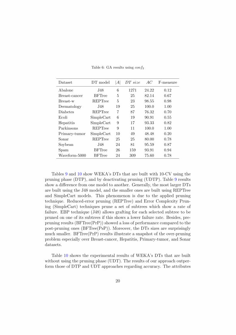
Table 6: GA results using conf2

Dataset DT model |A| DT size AC F-measure

Abalone J48 6 1271 24.22 0.12Breast-cancer BFTree 5 25 82.14 0.67Breast-w REPTree 5 23 98.55 0.98Dermatology J48 19 25 100.0 1.00Diabetes REPTree 7 87 76.32 0.70Ecoli SimpleCart 6 19 90.91 0.55Hepatitis SimpleCart 9 17 93.33 0.82Parkinsons REPTree 9 11 100.0 1.00Primary-tumor SimpleCart 10 49 48.48 0.20Sonar REPTree 25 25 80.00 0.78Soybean J48 24 81 95.59 0.87Spam BFTree 26 159 93.91 0.94Waveform-5000 BFTree 24 309 75.60 0.78

Tables 9 and 10 show WEKA’s DTs that are built with 10-CV using thepruning phase (DTP), and by deactivating pruning (UDTP). Table 9 resultsshow a di↵erence from one model to another. Generally, the most larger DTsare built using the J48 model, and the smaller ones are built using REPTreeand SimpleCart models. This phenomenon is due to the applied pruningtechnique. Reduced-error pruning (REPTree) and Error Complexity Prun-ing (SimpleCart) techniques prune a set of subtrees which show a rate offailure. EBP technique (J48) allows grafting for each selected subtree to bepruned on one of its subtrees if this shows a lower failure rate. Besides, pre-pruning results (BFTree(PrP)) showed a loss of performance compared to thepost-pruning ones (BFTree(PsP)). Moreover, the DTs sizes are surprisinglymuch smaller. BFTree(PrP) results illustrate a snapshot of the over-pruningproblem especially over Breast-cancer, Hepatitis, Primary-tumor, and Sonardatasets.

Table 10 shows the experimental results of WEKA’s DTs that are builtwithout using the pruning phase (UDT). The results of our approach outper-form those of DTP and UDT approaches regarding accuracy. The attributes

20

Table 7: GA results using conf3

Dataset DT model |A| DT size AC F-measure

Abalone REPTree 7 1288 22.30 0.14Breast-cancer SimpleCart 6 13 82.14 0.72Breast-w J48 7 11 98.55 0.98Dermatology SimpleCart 19 19 97.22 0.97Diabetes REPTree 7 107 80.26 0.74Ecoli SimpleCart 4 35 90.91 0.56Hepatitis SimpleCart 6 11 86.67 0.83Parkinsons SimpleCart 11 17 94.74 0.88Primary-tumor BFTree 9 67 54.54 0.20Sonar REPTree 29 23 90.00 0.89Soybean BFTree 19 103 95.59 0.85Spam BFTree 34 199 93.48 0.93Waveform-5000 REPTree 25 391 77.80 0.78

and the training samples that are used inthe GA process are far smaller thanthe ones used to build DTP and UDT models. The sizes of the generated DTsare smaller than those of UDT, and larger than those of DTP. Furthermore,the approach handles the over-pruning on tested datasets.

Figure 7 plots a comparison between the average AC results of the GAapproach UDT and DTP.

Dataset

abalon

e

brea

st-c

ance

r

brea

st-w

derm

atolog

y

diab

etes

ecoli

hepa

titis

park

inso

ns

prim

ary-

tum

or

sona

r

soyb

ean

spam

wav

efor

m-5

000

Acc

ura

cy (

%)

0

20

40

60

80

100

GAUDTDTP

Figure 7: The average DTs AC performances

21

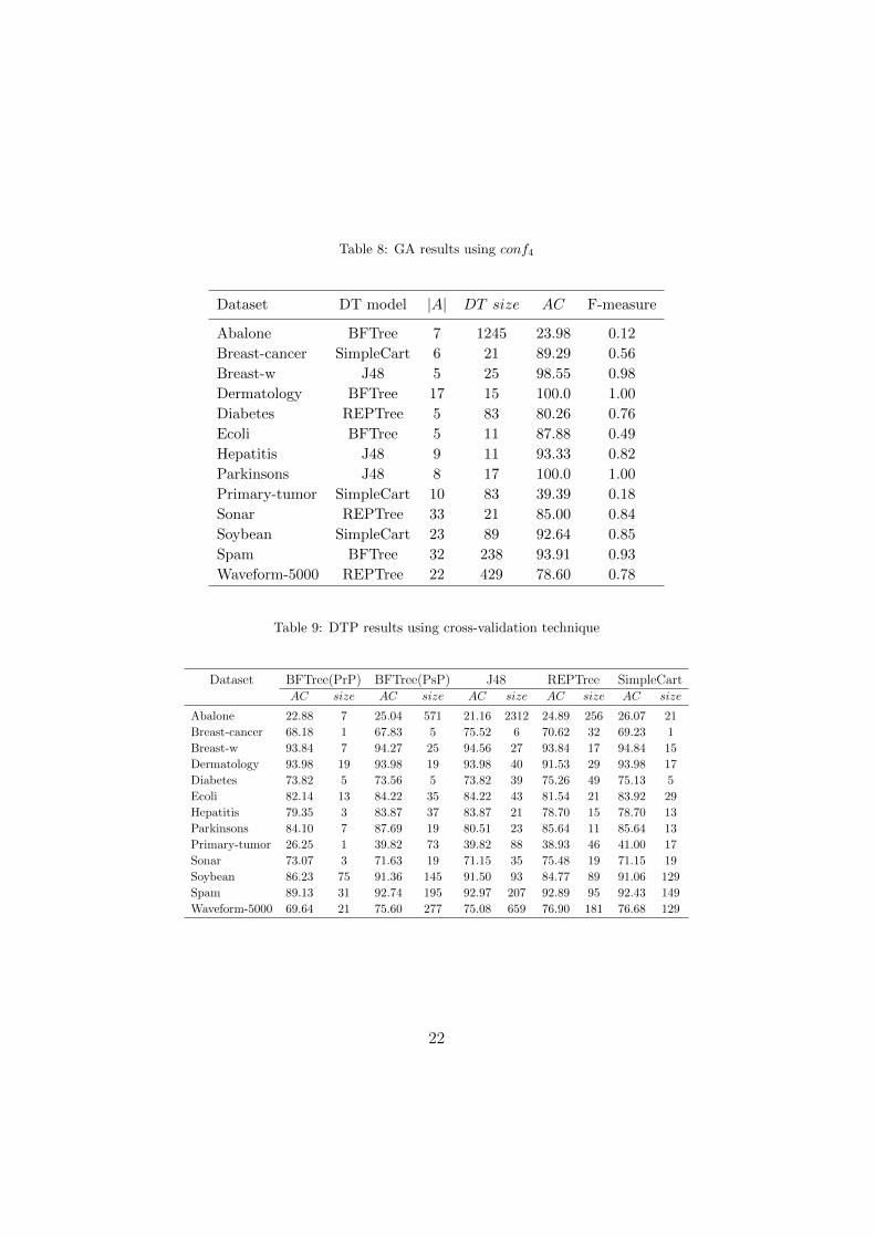
Table 8: GA results using conf4

Dataset DT model |A| DT size AC F-measure

Abalone BFTree 7 1245 23.98 0.12Breast-cancer SimpleCart 6 21 89.29 0.56Breast-w J48 5 25 98.55 0.98Dermatology BFTree 17 15 100.0 1.00Diabetes REPTree 5 83 80.26 0.76Ecoli BFTree 5 11 87.88 0.49Hepatitis J48 9 11 93.33 0.82Parkinsons J48 8 17 100.0 1.00Primary-tumor SimpleCart 10 83 39.39 0.18Sonar REPTree 33 21 85.00 0.84Soybean SimpleCart 23 89 92.64 0.85Spam BFTree 32 238 93.91 0.93Waveform-5000 REPTree 22 429 78.60 0.78

Table 9: DTP results using cross-validation technique

Dataset BFTree(PrP) BFTree(PsP) J48 REPTree SimpleCartAC size AC size AC size AC size AC size

Abalone 22.88 7 25.04 571 21.16 2312 24.89 256 26.07 21Breast-cancer 68.18 1 67.83 5 75.52 6 70.62 32 69.23 1Breast-w 93.84 7 94.27 25 94.56 27 93.84 17 94.84 15Dermatology 93.98 19 93.98 19 93.98 40 91.53 29 93.98 17Diabetes 73.82 5 73.56 5 73.82 39 75.26 49 75.13 5Ecoli 82.14 13 84.22 35 84.22 43 81.54 21 83.92 29Hepatitis 79.35 3 83.87 37 83.87 21 78.70 15 78.70 13Parkinsons 84.10 7 87.69 19 80.51 23 85.64 11 85.64 13Primary-tumor 26.25 1 39.82 73 39.82 88 38.93 46 41.00 17Sonar 73.07 3 71.63 19 71.15 35 75.48 19 71.15 19Soybean 86.23 75 91.36 145 91.50 93 84.77 89 91.06 129Spam 89.13 31 92.74 195 92.97 207 92.89 95 92.43 149Waveform-5000 69.64 21 75.60 277 75.08 659 76.90 181 76.68 129

22

Table 10: UDTP results using cross-validation technique

Dataset BFTree J48 REPTree SimpleCartAC size AC size AC size AC size

Abalone 21.54 2131 20.58 2540 20.90 2327 21.35 2147Breast-cancer 60.48 69 69.58 179 66.78 212 60.48 69Breast-w 94.27 55 93.70 45 94.27 55 94.27 55Dermatology 94.26 19 94.53 44 90.16 61 94.26 19Diabetes 71.74 157 72.65 43 70.31 187 71.74 159Ecoli 83.92 37 83.63 51 82.73 41 83.92 37Hepatitis 80.00 49 80.64 31 78.06 23 80.00 49Parkinsons 87.17 19 80.51 23 84.10 23 87.17 19Primary-tumor 39.23 155 40.41 123 35.39 132 39.23 157Sonar 70.67 27 69.71 35 73.07 35 70.67 27Soybean 91.80 167 91.36 175 89.60 137 91.80 167Spam 92.76 227 92.58 379 92.45 291 92.76 227Waveform-5000 75.22 531 74.94 677 75.16 685 75.40 531

4.2. Comparison with existing state-of-the-art classifiers

To further evaluate the robustness of the proposedGA schema for DT con-struction, we compare our results with two state-of-the-art classifiers namelyNaive Bayes (NB), and Support Vector Machine (SVM). For the two clas-sifiers, we use WEKA’s implementation with the default parameters. ForSVM, we use two configurations. The first one is based on a Polynomialkernel denoted SVM(POLY) and the second one is based on a Radial BasisFunction kernel denoted SVM(RBF).

Table 11 shows the obtained accuracy results, and it clearly demonstratesthe robustness of the proposed approach compared to well established clas-sifiers. As illustrated on Figure 8, our approach outperforms the otherones in eight datasets out of thirteen. However, NB, SVM(POLY ) andSVM(RBF ) scored best respectively for one, three, and one dataset out ofthe thirteen.

Table 12 presents the F-measure evaluation results for each classifier.These results support the domination of the proposed approach where the

23

Table 11: GA DTs accuracy vs. NB and SVM classifiers

Dataset NB SVM(POLY) SVM(RBF) GAAbalone 22.45 25.64 19.40 24.34Breast-cancer 76.43 67.50 60.00 78.57Breast-w 96.23 96.67 93.77 98.91Dermatology 95.83 95.57 94.17 98.06Diabetes 75.00 76.58 76.05 77.10Ecoli 83.33 84.24 87.27 84.85Hepatitis 81.33 82.00 86.67 93.33Parkinsons 69.47 89.47 93.16 93.68Primary-tumor 45.46 42.73 41.21 44.85Sonar 65.50 74.50 77.00 79.50Soybean 93.24 93.38 75.41 93.38Spam 80.02 90.24 85.54 92.89Waveform-5000 79.30 86.92 97.38 76.56

Dataset

Abalone

Breas

t-can

cer

Breas

t-w

Der

mat

olog

y

Diabe

tes

Ecoli

Hep

atitis

Parkins

ons

Primar

y-tu

mor

Sonar

Soybe

an

Spam

Wav

efor

m-5

000

Acc

ura

cy (

%)

0

20

40

60

80

100

NBSVM(poly)SVM(RBF)GA

Figure 8: The GA DTs AC performances vs. NB, SVM(POLY ) and SVM(RBF )

latter outperforms its competitor approaches in seven datasets. However,NB, SVM(POLY ) and SVM(RBF ) scored best each in two datasets re-spectively.

4.3. Comparison with other evolutionary DT approaches

In this section, we compare our GA scheme for constructing an improvedDT to Ant-Tree-Miner [39] that uses an ant colony optimization algorithmfor inducing an optimized DT. In [39], the authors showed that Ant-Tree-Miner outperformed multiple decision tree construction approaches including

24

Table 12: GA DTs F-measure vs. NB and SVM classifiers

Dataset NB SVM (poly) SVM (RBF) GA

Abalone 0.086 0.062 0.026 0.127Breast-cancer 0.681 0.541 0.550 0.546Breast-w 0.958 0.964 0.932 0.987Dermatology 0.903 0.951 0.910 0.977Diabetes 0.718 0.709 0.721 0.709Ecoli 0.494 0.484 0.542 0.517Hepatitis 0.703 0.638 0.730 0.818Parkinsons 0.662 0.819 0.907 0.919Primary-tumor 0.182 0.165 0.177 0.167Sonar 0.640 0.726 0.758 0.771Soybean 0.821 0.870 0.842 0.841Spam 0.794 0.896 0.692 0.924Waveform-5000 0.780 0.870 0.854 0.763

state-of-the-art algorithms like C4.5 and CART as well as other evolution-ary decision tree construction approaches like cACDT [7]. The comparisonbetween the two algorithms will focus on accuracy and runtime. Table 13presents the comparison results. We note that Ant-Tree-Miner required hightraining runtime for some datasets and it did not finish within 24 hours.Thus, we denote the accuracy and runtime by ”- - -” in those cases.

The comparison in Table 13 clearly indicates that the DTs generated byour approach are more accurate than those generated by Ant-Tree-Miner,except in the case of Ecoli dataset. According to the runtime results, theproposed GA still outperforms the Ant-Tree-Miner. The results show thatAnt-Tree-Miner could not finish within 24h for Abalone, Soybean, Spam andWaveform-5000 datasets. Moreover, Ant-Tree-Miner required considerablymore running time to construct its DTs for six datasets from the nine forwhich it finished running within 24h.

4.4. Fault diagnosis in a rotating machine experimental results

We now consider the generation of DTs using our approach for the prob-lem of fault diagnosis in rotating machines. The condition-monitoring taskmay be naturally treated like a classification task, where each condition (good

25

Table 13: Accuracy and runtime of GA DTs vs. Ant-Tree-Miner

Dataset GA Ant-Tree-Miner

AC Runtime AC Runtime

Abalone 23.14 4702 s - - - - - -Breast-cancer 78.57 373 s 72.70 482 sBreast-w 98.91 230 s 95.42 1126 sDermatology 98.06 2019 s 94.25 945 sDiabetes 77.10 324 s 73.57 37668 sEcoli 84.85 196 s 85.80 1028 sHepatitis 93.33 342 s 83.12 244 sParkinsons 93.68 377 s 90.79 345 sPrimary-tumor 44.85 375 s 44.26 11265 sSonar 79.50 1033 s 66.81 1130 sSoybean 93.38 3212 s - - - - - -Spam 92.89 10354 s - - - - - -Waveform-5000 76.56 7501 s - - - - - -

and defective) is considered as a class. This is performed by extracting in-formation from vibration sensors to indicate the machine’s current condition(class). The proposed evolutionary approach is validated on a dataset thatwas presented in [29]. This dataset is constructed using a test ring (notedring data) under a normal operating condition and with three di↵erent faults:mass imbalance, gear fault, and faulty belt. The dataset is characterized asfollow:

• ring data: 4 classes, 55 attributes, 420 instances, 105 instances for eachclass, and 75% Base Error.

Table 14 shows the classification results of the proposed approach over thering data. In general, the results are good where the AC illustrates perfor-mances between 97.62 and 100%, and the F-measure performances are be-tween 0.97 and 1.00. The sizes of the DTs are the between 21 and 25 nodes.Yet, the used subset of attributes shows an important reduction comparedto the total number of attributes which is 55.

Tables 15 and 16 show the experimental results with 10-CV by consideringthe pruned/unpruned WEKA’s DTs.

26

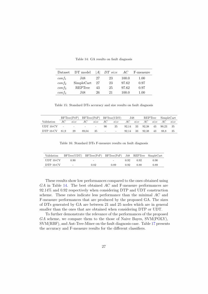
Table 14: GA results on fault diagnosis

Dataset DT model |A| DT size AC F-measure

conf1 J48 27 23 100.0 1.00conf2 SimpleCart 27 23 97.62 0.97conf3 REPTree 43 25 97.62 0.97conf4 J48 26 21 100.0 1.00

Table 15: Standard DTs accuracy and size results on fault diagnosis

BFTree(PrP) BFTree(PsP) BFTree(UDT) J48 REPTree SimpleCartValidation AC size AC size AC size AC size AC size AC size

UDT 10-CV - - - - 90 35 92,14 33 92,38 43 90,23 35

DTP 10-CV 81,9 29 89,04 35 - - 92,14 33 92,38 43 88,8 35

Table 16: Standard DTs F-measure results on fault diagnosis

Validation BFTree(UDT) BFTree(PrP) BFTree(PsP) J48 REPTree SimpleCart

UDT 10-CV 0.90 - - 0.92 0.92 0.90

DTP 10-CV - 0.82 0.89 0.92 0.88 0.89

These results show low performances compared to the ones obtained usingGA in Table 14. The best obtained AC and F-measure performances are92.14% and 0.92 respectively when considering DTP and UDT constructionscheme. These rates indicate less performance than the minimal AC andF-measure performances that are produced by the proposed GA. The sizesof DTs generated by GA are between 21 and 25 nodes which are in generalsmaller than the ones that are obtained when considering DTP or UDT.

To further demonstrate the relevance of the performances of the proposedGA scheme, we compare them to the those of Naive Bayes, SVM(POLY),SVM(RBF), and Ant-Tree-Miner on the fault diagnosis case. Table 17 presentsthe accuracy and F-measure results for the di↵erent classifiers.

27

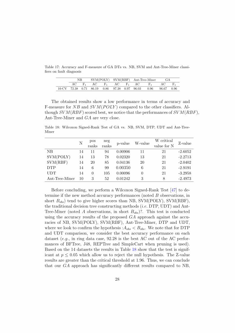
Table 17: Accuracy and F-measure of GA DTs vs. NB, SVM and Ant-Tree-Miner classi-fiers on fault diagnosis

NB SVM(POLY) SVM(RBF) Ant-Tree-Miner GAAC F1 AC F1 AC F1 AC F1 AC F1

10-CV 72.38 0.71 86.19 0.86 97.38 0.97 96.03 0.96 96.67 0.96

The obtained results show a low performance in terms of accuracy andF-measure for NB and SVM(POLY ) compared to the other classifiers. Al-though SVM(RBF ) scored best, we notice that the performances of SVM(RBF ),Ant-Tree-Miner and GA are very close.

Table 18: Wilcoxon Signed-Rank Test of GA vs. NB, SVM, DTP, UDT and Ant-Tree-Miner

Nposranks

negranks

p-value W-valueW criticalvalue for N

Z-value

NB 14 11 94 0.00906 11 21 -2.6052SVM(POLY) 14 13 78 0.02320 13 21 -2.2713SVM(RBF) 14 20 85 0.04136 20 21 -2.0402DTP 14 6 99 0.00350 6 21 -2.9191UDT 14 0 105 0.00096 0 21 -3.2958Ant-Tree-Miner 10 3 52 0.01242 3 8 -2.4973

Before concluding, we perform a Wilcoxon Signed-Rank Test [47] to de-termine if the new method accuracy performances (noted B observations, inshort B

obs

) tend to give higher scores than NB, SVM(POLY), SVM(RBF),the traditional decision tree constructing methods (i.e. DTP, UDT) and Ant-Tree-Miner (noted A observations, in short B

obs

)?. This test is conductedusing the accuracy results of the proposed GA approach against the accu-racies of NB, SVM(POLY), SVM(RBF), Ant-Tree-Miner, DTP and UDT,where we look to confirm the hypothesis :A

obs

< Bobs

. We note that for DTPand UDT comparison, we consider the best accuracy performance on eachdataset (e.g., in ring data case, 92.28 is the best AC out of the AC perfor-mances of BFTree, J48, REPTree and SimpleCart when pruning is used).Based on the 14 datasets the results in Table 18 show that the test is signif-icant at p 0.05 which allow us to reject the null hypothesis. The Z-valueresults are greater than the critical threshold at 1.96. Thus, we can concludethat our GA approach has significantly di↵erent results compared to NB,

28

SVM(POLY), SVM(RBF), DTP, UDT and Ant-Tree-Miner. Therefore, theGA approach is the best under the confidence of 95%.

5. Conclusion and further study

The popularity of DTs is strongly related to their simplicity, ease of un-derstanding, and closeness to human reasoning. However, each DT modelhas its specificities, and many choices still need to be made making it a com-binatorial problem. In this paper, we proposed to use good sub-training andsub-testing samples and only a subset of pertinent attributes to constructan optimal DT with respect to the input dataset. We also considered theuse of the prune/unpruned decision as well as some other parameters whenconstructing the optimal DT. We proposed the usage of a GA scheme inorder to overcome the high runtime and computational cost that are dueto the combinatorial nature of the problem of choosing the best settings.Experimental results on 13 benchmark datasets showed that the proposedapproach allows constructing e�cient DTs that o↵er very high accuracy andF-measure results while e�ciently reducing the size of the generated trees.Moreover, the proposed GA scheme was applied on a real-world application offault diagnosis in rotating machines. The obtained results also demonstratedthe e↵ectiveness and e�ciency of our approach in terms of complexity andclassification accuracy of the constructed DTs. One of the main drawbacksof this work is that the encoding of the dataset attributes is in the form ofa binary sequence where each bit represents the presence or the absence ofthe attribute in the GA candidate solution. In cases were the number ofattributes is extremely large, the GA could su↵er computational problemsmainly due to the size of the binary encoding vector. An important futureextension could be to propose an alternative encoding representation vectorthat requires a small size and that could e�ciently handle large dimensionsin a compressed way in order to overcome memory and computational limi-tations.

References

[1] S. Aksoy, K. Koperski, C. Tusk, G. Marchisio, and J.C. Tilton. Learn-ing bayesian classifiers for scene classification with a visual grammar.Geoscience and Remote Sensing, IEEE Transactions on, 43(3):581–589,2005.

29

[2] S. Aridhi, H. Sghaier, M. Zoghlami, M. Maddouri, and E.M. Nguifo.Prediction of ionizing radiation resistance in bacteria using a multipleinstance learning model. Journal of Computational Biology, 23(1):10–20,2016.

[3] R.C. Barros, M.P. Basgalupp, A.A. Freitas, and A.C.P.L.F. De Car-valho. Evolutionary design of decision-tree algorithms tailored to mi-croarray gene expression data sets. IEEE Transactions on EvolutionaryComputation, 18(6):873–892, 2014.

[4] P. Bermejo, L. de la Ossa, J.A. Gamez, and J.M. Puerta. Fast wrapperfeature subset selection in high-dimensional datasets by means of filterre-ranking. Knowledge-Based Systems, 25(1):35–44, 2012.

[5] C. Blake and C.J. Merz. Uci repository of machine learning databases[http://www. ics. uci. edu/˜ mlearn/mlrepository. html]. irvine, ca: Uni-versity of california. Department of Information and computer science,55, 1998.

[6] J. Bobadilla, F. Ortega, A. Hernando, and A. Gutierrez. Recommendersystems survey. Knowledge-Based Systems, 46:109 – 132, 2013.

[7] U. Boryczka and J. Kozak. An adaptive discretization in the acdt algo-rithm for continuous attributes. In International Conference on Com-putational Collective Intelligence, pages 475–484. Springer, 2011.

[8] L. Breiman. Bagging predictors. Machine learning, 24(2):123–140, 1996.

[9] L. Breiman, J. Friedman, C.J. Stone, and R.A. Olshen. Classificationand regression trees. CRC press, 1984.

[10] S.H. Cha and C. Tappert. A genetic algorithm for constructing compactbinary decision trees. Journal of pattern recognition research, 4(1):1–13,2009.

[11] B. Chandra and P.P. Varghese. Moving towards e�cient decision treeconstruction. Information Sciences, 179(8):1059–1069, 2009.

[12] J. Chen, X. Wang, and J. Zhai. Pruning decision tree using geneticalgorithms. In Artificial Intelligence and Computational Intelligence,2009. AICI’09. International Conference on, volume 3, pages 244–248.IEEE, 2009.

30

[13] K.M. Chung, W.C. Kao, C.L. Sun, L.L Wang, and C.J Lin. Radiusmargin bounds for support vector machines with the rbf kernel. Neuralcomputation, 15(11):2643–2681, 2003.

[14] R. Conforti, M. de Leoni, M. La Rosa, W.M.P. van der Aalst, andA.H.M. ter Hofstede. A recommendation system for predicting risksacross multiple business process instances. Decision Support Systems,69:1–19, 2015.

[15] UniProt Consortium et al. Uniprot: a hub for protein information.Nucleic Acids Research, 43(D1):D204, 2014.

[16] C. Cortes and V. Vapnik. Support-vector networks. Machine learning,20(3):273–297, 1995.

[17] E. De la Hoz, E. de la Hoz, A. Ortiz, J. Ortega, and A. Martınez-Alvarez. Feature selection by multi-objective optimisation: Applica-tion to network anomaly detection by hierarchical self-organising maps.Knowledge-Based Systems, 71:322–338, 2014.

[18] W. Dhifli and A.B. Diallo. Protnn: fast and accurate protein 3d-structure classification in structural and topological space. BioDataMining, 9(1):30, 2016.

[19] W. Dhifli, R. Saidi, and E.M. Nguifo. Smoothing 3d protein structuremotifs through graph mining and amino acid similarities. Journal ofComputational Biology, 21(2):162–172, 2014.

[20] T.G. Dietterich. An experimental comparison of three methods for con-structing ensembles of decision trees: Bagging, boosting, and random-ization. Machine learning, 40(2):139–157, 2000.

[21] F. Esposito, D. Malerba, G. Semeraro, and J.A. Kay. A comparativeanalysis of methods for pruning decision trees. Pattern Analysis andMachine Intelligence, IEEE Transactions on, 19(5):476–491, 1997.

[22] J. Gehrke, V. Ganti, R. Ramakrishnan, and W.Y. Loh. Boatoptimisticdecision tree construction. In ACM SIGMOD Record, volume 28, pages169–180. ACM, 1999.

31

[23] A.E. Gutierrez-Rodrıguez, J.F Martınez-Trinidad, M. Garcıa-Borroto,and J.A. Carrasco-Ochoa. Mining patterns for clustering on numericaldatasets using unsupervised decision trees. Knowledge-Based Systems,82:70–79, 2015.

[24] I. Guyon, J. Weston, S. Barnhill, and V. Vapnik. Gene selection forcancer classification using support vector machines. Machine learning,46(1-3):389–422, 2002.

[25] M. Hall, E. Frank, G. Holmes, B. Pfahringer, P. Reutemann, and I.H.Witten. The weka data mining software: an update. ACM SIGKDDexplorations newsletter, 11(1):10–18, 2009.

[26] S. Haykin and N. Network. A comprehensive foundation. Neural Net-works, 2(2004), 2004.

[27] T.P. Hong, Y.L. Liou, S.L. Wang, and B. Vo. Feature selection andreplacement by clustering attributes. Vietnam Journal of ComputerScience, 1(1):47–55, 2014.

[28] N.E.I. Karabadji, I. Khelf, H. Seridi, and L. Laouar. Genetic optimiza-tion of decision tree choice for fault diagnosis in an industrial ventila-tor. In Condition monitoring of machinery in non-stationary operations,pages 277–283. Springer, 2012.

[29] N.E.I. Karabadji, H. Seridi, I. Khelf, N. Azizi, and R. Boulkroune. Im-proved decision tree construction based on attribute selection and datasampling for fault diagnosis in rotating machines. Engineering Applica-tions of Artificial Intelligence, 35:71–83, 2014.

[30] N.E.I. Karabadji, H. Seridi, I. Khelf, and L. Laouar. Decision tree se-lection in an industrial machine fault diagnostics. In Model and DataEngineering, pages 129–140. Springer, 2012.

[31] K.M. Kim, J.J. Park, M.H. Song, I.C. Kim, and C.Y. Suen. Binarydecision tree using genetic algorithm for recognizing defect patterns ofcold mill strip. In Advances in Artificial Intelligence, pages 461–466.Springer, 2004.

[32] Y. LeCun, Y. Bengio, and G. Hinton. Deep learning. Nature,521(7553):436–444, 2015.

32

[33] D.D. Lewis. Naive (bayes) at forty: The independence assumption in in-formation retrieval. In European conference on machine learning, pages4–15. Springer, 1998.

[34] H. Lu, R. Setiono, and H. Liu. E↵ective data mining using neuralnetworks. Knowledge and Data Engineering, IEEE Transactions on,8(6):957–961, 1996.

[35] M. Macas, L. Lhotska, E. Bakstein, D. Novak, J. Wild, T. Sieger,P. Vostatek, and R. Jech. Wrapper feature selection for small sam-ple size data driven by complete error estimates. Computer methodsand programs in biomedicine, 108(1):138–150, 2012.

[36] J. Mingers. An empirical comparison of pruning methods for decisiontree induction. Machine learning, 4(2):227–243, 1989.

[37] A. Mukhopadhyay, U. Maulik, S. Bandyopadhyay, and C.A.C. Coello. Asurvey of multiobjective evolutionary algorithms for data mining: Parti. IEEE Transactions on Evolutionary Computation, 18(1):4–19, 2014.

[38] T. Niblett and I. Bratko. Learning decision rules in noisy domains. InProceedings of Expert Systems’ 86, The 6Th Annual Technical Confer-ence on Research and development in expert systems III, pages 25–34.Cambridge University Press, 1987.

[39] F.E.B. Otero, A.A. Freitas, and C.G. Johnson. Inducing decision treeswith an ant colony optimization algorithm. Applied Soft Computing,12(11):3615–3626, 2012.

[40] S. Pei, Q. Hu, and C. Chen. Multivariate decision trees with monotonic-ity constraints. Knowledge-Based Systems, 112:14–25, 2016.

[41] S. Piramuthu. Input data for decision trees. Expert Systems with appli-cations, 34(2):1220–1226, 2008.

[42] J.R. Quinlan. Simplifying decision trees. International journal of man-machine studies, 27(3):221–234, 1987.

[43] J.R. Quinlan. C4. 5: Programming for machine learning. Morgan Kau↵-mann, page 38, 1993.

33

[44] J. Schmidhuber. Deep learning in neural networks: An overview. NeuralNetworks, 61:85–117, 2015.

[45] M. Srinivas and L.M. Patnaik. Genetic algorithms: A survey. Computer,27(6):17–26, 1994.

[46] G. Stein, B. Chen, A.S. Wu, and K.A. Hua. Decision tree classifier fornetwork intrusion detection with ga-based feature selection. In Proceed-ings of the 43rd annual Southeast regional conference-Volume 2, pages136–141. ACM, 2005.

[47] F. Wilcoxon, S.K. Katti, and R.A. Wilcox. Critical values and probabil-ity levels for the wilcoxon rank sum test and the wilcoxon signed ranktest. Selected tables in mathematical statistics, 1:171–259, 1970.

[48] Q. Wu, Y. Ye, H. Zhang, M.K Ng, and S.S. Ho. Forestexter: an e�cientrandom forest algorithm for imbalanced text categorization. Knowledge-Based Systems, 67:105–116, 2014.

[49] S. Xiang, F. Nie, G. Meng, C. Pan, and C. Zhang. Discriminativeleast squares regression for multiclass classification and feature selec-tion. IEEE transactions on neural networks and learning systems,23(11):1738–1754, 2012.

34